giirr model solutions - soa.org model solutions spring 2016 1. ... the rate level relative value for...

GI IRR Spring 2016 Solutions

GIIRR Model Solutions

Spring 2016

1. Learning Objectives: 1. The candidate will understand the key considerations for general insurance

actuarial analysis.

Learning Outcomes:

(1k) Estimate written, earned and unearned premiums.

(1l) Adjust historical earned premiums to current rate levels.

Sources:

Fundamentals of General Insurance Actuarial Analysis, J. Friedland, Chapters 11 and 12.

Commentary on Question:

This question tests the candidate’s ability to make correct calculations of earned

premium. The candidate also needs to understand earned premiums adjusted to current

rate level that are used when projecting expected claim ratios, as well as calculating the

weighted average rate level when a new discount is introduced.

Solution:

(a) Calculate the policy year 2015 earned premium evaluated as of December 31,

2016.

2015 policy year earned premium = 12×2,000 = 24,000

(b) Calculate the calendar year 2015 earned premium.

Commentary on Question: There are two approaches that can be used. Candidates could either assume that

the policies written in the first half of the year are renewed during the second half

of the year, or candidates could answer the question considering only new policy

writings during the year.

Solution for assuming only new policy writings during the year:

The policy written on January 1 expires on June 30, and is therefore

earned for six months in calendar year (CY) 2015.

Similarly, the policies written on February 1, March 1, April 1, May 1,

June 1, and July 1 are all earned for six months in CY 2015.

The policy written on August 1 is earned for five months in CY 2015.


1. Continued

The policy written on September 1 is earned for four months in CY 2015.

The policy written on October 1 is earned for three months in CY 2015.

The policy written on November 1 is earned for two months in CY 2015.

The policy written on December 1 is earned for one month in CY 2015.

CY 2015 earned premium = 2,000 × (6/6 + 6/6 + 6/6 + 6/6 + 6/6 + 6/6 + 6/6 + 5/6

+ 4/6 + 3/6 + 2/6 + 1/6) = 19,000

(c) Calculate the premium on-level factors for 2011 and 2012 used to project

expected claim ratios for reserving purposes as of December 31, 2015.

Commentary on Question: Note that the six-month policy terms cause the height of the triangles to be twice

the base.

% at Rate Level in CY

Rate Level

Rate Level

Relative Value 2011 2012 2015

A 1.0000 93.75% 6.25%

B 1.0800 6.25% 68.75%

C 1.1232 25.00%

D 1.0446 6.25%

E 1.1699 87.50%

F 1.2401 6.25%

Weighted average rate level 1.0050 1.0858 1.1665

e.g., % at rate level C in CY 2012 = ½ × ½ × 1 = 25%

Weighted average rate level = sumproduct of rate level relative value and % at

rate level in CY (e.g., 1.0050 = 1.0000 × 93.75% + 1.0800 × 6.25%).

Premium on-level factors that are used to project expected claim ratios for

reserving purposes as of December 31, 2015 need to use the weighted average

rate level for 2015 as the numerator.

2011 2012 2013 2014 2015 2016

A B C D E F

+8% +4% -7% +12% +6%


1. Continued

Premium on-level factor for 2011 = 1.1665

1.1611.0050

Premium on-level factor for 2012 = 1.1665

1.0741.0858

(d) Calculate the weighted average rate level for 2012.

Average discount is 40% × 10% = 4%.

2012 can be represented using the following graph:

The rate level relative value for A is 1.

The rate level relative value for B is 1.08.

The rate level relative value for C is 1.08×0.96 = 1.0368.

The rate level relative value for D is 1.08×1.04×0.96 = 1.0783.

The areas of each shape are as follows:

A ½ × ½ × ¼ = 6.25%

B 0.5 – 0.0625 = 43.75%

C ½ × ½ × 1 = 25%

D ½ × ½ × 1 = 25%

The weighted average rate level for 2012 = (1×0.0625) + (1.08×0.4375) +

(1.0368×0.25) + (1.0783×0.25) = 1.0638.

2011 2012 2013

A C D

B

+8% +4% rate change (diagonal)

10% new discount (vertical)


2. Learning Objectives: 2. The candidate will understand how to calculate projected ultimate claims and

claims-related expenses.

3. The candidate will understand financial reporting of claim liabilities and premium

liabilities.

6. The candidate will understand the need for monitoring results.

Learning Outcomes:

(2b) Estimate ultimate claims using various methods: development method, expected

method, Bornhuetter Ferguson method, Cape Cod method, frequency-severity

methods, Berquist-Sherman methods.

(2c) Estimate claims-related expenses and recoveries.

(3b) Estimate unpaid unallocated loss adjustment expenses using ratio and count-based

methods.

(3d) Evaluate the estimates of ultimate claims to determine claim liabilities for

financial reporting.

(6b) Analyze actual claims experience relative to expectations.

Sources:

Fundamentals of General Insurance Actuarial Analysis, J. Friedland, Chapters 14, 17, 22,

23, and 36.


This question tests the candidate’s understanding of comparing actual vs. expected

claims, estimating IBNR reserves using the development method, the Bornhuetter

Ferguson method, and the Benktander method, and estimating unpaid ULAE using the

Mango and Allen smoothing adjustment.

Solution:

(a) Calculate the difference between actual paid claims and expected paid claims for

each accident year.

(1) (2) (3) = (2)×0.65 (4) (5) = (3)/(4) (6) = (1) – (5)

Accident

Year

Actual

Paid

Claims

Earned

Premium

A Priori

Expected

Claims

Paid

CDF

Expected

Paid Claims

Actual vs.

Expected

2013 49,000 90,000 58,500 1.20 48,750 250

2014 40,500 100,000 65,000 1.60 40,625 –125

2015 40,000 110,000 71,500 2.00 35,750 4,250

Total 4,375


2. Continued

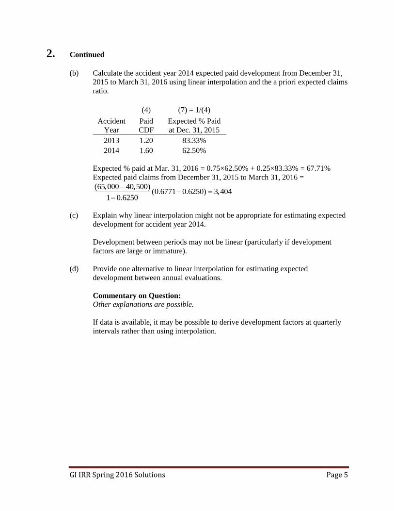
(b) Calculate the accident year 2014 expected paid development from December 31,

2015 to March 31, 2016 using linear interpolation and the a priori expected claims

ratio.

(4) (7) = 1/(4)

Accident

Year

Paid

CDF

Expected % Paid

at Dec. 31, 2015

2013 1.20 83.33%

2014 1.60 62.50%

Expected % paid at Mar. 31, 2016 = 0.75×62.50% + 0.25×83.33% = 67.71%

Expected paid claims from December 31, 2015 to March 31, 2016 =

(65,000 40,500)(0.6771 0.6250) 3,404

1 0.6250

(c) Explain why linear interpolation might not be appropriate for estimating expected

development for accident year 2014.

Development between periods may not be linear (particularly if development

factors are large or immature).

(d) Provide one alternative to linear interpolation for estimating expected

development between annual evaluations.

Commentary on Question: Other explanations are possible.

If data is available, it may be possible to derive development factors at quarterly

intervals rather than using interpolation.


2. Continued

(e) Calculate estimated IBNR reserves for each accident year using the following

methods applied to paid claim data:

(i) Development method

(ii) Bornhuetter Ferguson method

(iii) Benktander method, one iteration

(1) (3) = (2)×0.65 (4) (7) = 1/(4) (8) = 1 – (7)

Accident

Year

Actual

Paid

Claims

A Priori

Expected

Claims Paid CDF 1/CDF 1 – 1/CDF

2013 49,000 58,500 1.20 0.8333 0.1667

2014 40,500 65,000 1.60 0.6250 0.3750

2015 40,000 71,500 2.00 0.5000 0.5000

(9) = (1)(4) (10) = (1) + (8)(3) (11) = (1) + (8)(10)

Ultimate Claims

Accident

Year

Development

Method

Bornhuetter

Ferguson Method

Benktander

Method

2013 58,800 58,752 58,794

2014 64,800 64,875 64,828

2015 80,000 75,750 77,875

(12) (13) = (9) – (12) (14) = (10) – (12) (15) = (11) – (12)

Estimated IBNR

Accident

Year

Actual

Reported

Claims

Development

Method

Bornhuetter

Ferguson Method

Benktander

Method

2013 54,000 4,800 4,752 4,794

2014 50,000 14,800 14,875 14,828

2015 45,000 35,000 30,750 32,875


2. Continued

(f) Describe one situation for which the development method might provide a better

estimate for the accident year 2015 IBNR reserves.


The development method might be more appropriate if accident year 2015 is

showing true deterioration.

(g) Describe one situation for which the Bornhuetter Ferguson method might provide

a better estimate for the accident year 2015 IBNR reserves.


The Bornhuetter Ferguson might be more appropriate if accident year 2015

includes unusual large loss(es) at 12 months which are not expected to develop

normally.

(h) Estimate accident year 2015 unpaid ULAE as of December 31, 2015 using the

classical paid-to-paid method, a multiplier of 50%, estimated IBNR from the

Bornhuetter Ferguson method (part (e) above), and the Mango-Allen smoothing

adjustment.

(1) (2) (3)

Calendar

Year

Actual Paid

ULAE

Expected

Paid Claims

Paid-to-Paid

Ratio

2013 5,580 55,800 10.0%

2014 5,890 60,100 9.8%

2015 7,100 69,600 10.2%

Selected paid-to-paid ratio = 10%

Bornhuetter Ferguson method IBNR = 30,750

Case estimate = 45,000 – 40,000 = 5,000

Unpaid ULAE = 10%×30,750 + 10%×0.5×5,000 = 3,325


2. Continued

(i) Identify four situations in which the Mango and Allen smoothing adjustment

should be considered in the selection of a ULAE ratio.


Situations include:

Sparse data

Volatile data

Long-tail lines of business

Changing exposure volume


3. Learning Objectives: 4. The candidate will understand trending procedures as applied to ultimate claims,

exposures and premiums.

Learning Outcomes:

(4b) Describe the influences on frequency and severity of changes in deductibles,

changes in policy limits, and changes in mix of business.

(4c) Choose trend rates and calculate trend factors for claims.

Sources:

Fundamentals of General Insurance Actuarial Analysis, J. Friedland, Chapter 25.


This question tests the candidate’s understanding of analyzing claim trend for long-tail

lines when the company has insufficient experience.

Solution:

(a) Identify one distinct consideration, for each of the following options:

(i) Use industry general insurance data for the applicable line of business and

jurisdiction.

(ii) Combine your company’s experience in one jurisdiction with your

company’s regional experience.

(iii) Combine your company’s experience with that of other affiliated insurers

in your group.

(i) Carefully review the applicability of external data and review the

obligations and guidance set out in the Standards.

(ii) Review the economic, legal, and regulatory environments that influence

frequency and severity.

(iii) Ensure there are similar operational policies, particularly with respect to

underwriting, claim management, and reinsurance OR Ensure there are

similarities in the types of exposures and products.

(b) Explain the effect this change will have on a claim trend analysis if there is no

adjustment in the historical data for the reform-driven policy change.

If the historical data is not adjusted, it will be higher than it should be (relative to

the now lower claims level). This will lead to a trend estimate that is lower than it

should be.


3. Continued

(c) Calculate the post-reform losses net of deductible using the claim distribution

above.

For the 5 claims of amount 50, reinstating the deductible gives a loss of 50 + 500

= 550. The 20% post-reform decrease takes it to 550(0.8) = 440. Reapplying the

deductible gives a claim of 0.

For the 10 claims of 500, reinstating the deductible gives a loss of 500 + 500 =

1,000. The 20% post-reform decrease takes it to 1,000(0.8) = 800. Reapplying

the deductible gives a claim of 800 – 500 = 300. With 10 claims the total loss is

3,000.

(d) Calculate the accident year 2015 pure premium trend factor.

The pure premium trend rate is (1 + 3%) × (1 – 1.5%) = 1.01455. The trending

period is 7/1/2015 to 1/1/2018, which is 2.5 years. See the diagram below for a

derivation. Thus the AY2015 pure premium trend factor is 1.014552.5 = 1.0368.

2015 2016 2017 2018 2019

Avg Acc Date = 7/1/2015 Avg Acc Date = 1/1/2018




Learning Outcomes:




Sources:



This question tests the candidate’s understanding of the Bornhuetter Ferguson method as

well as estimating ultimate salvage using the Bornhuetter Ferguson method.

Solution:

(a) Explain how the Bornhuetter Ferguson method of estimating ultimate claims

combines the development method and the expected method.

The observed experience is based on actual experience through the valuation date;

the balance of the ultimate value is based on the a priori estimate of the expected

method.

(b) Calculate the ultimate salvage for each accident year using the Bornhuetter

Ferguson method.

(1) (2) (3) (4) (5) = (1)(4)

Accident

Year

Reported

Salvage

Age-to-Age

Development

Factors

Ultimate

Claims

Age-to-

Ultimate

Development

Factors

Projected

Ultimate

Based on

Reported

2012 62,000 1.00 230,100 1.000 62,000

2013 66,000 0.99 229,400 0.990 65,340

2014 65,000 0.98 232,700 0.970 63,050

2015 67,000 0.95 239,200 0.922 61,774

Note: Column (4) = Cumulative product of column (2).

e.g., 1.00×0.99×0.98×0.95 = 0.922


4. Continued

(6) = 27%×(3) (7) = 1 – 1/(4) (8) = (6)(7) (9) = (1)+(8)

Accident

Year

Expected

Salvage

Expected %

Undeveloped

Expected

Salvage

Undeveloped

Projected

Ultimate

Salvage

2012 62,127 0.0% 0 62,000

2013 61,938 –1.0% –619 65,381

2014 62,829 –3.1% –1,948 63,052

2015 64,584 –8.5% –5,490 61,510

(c) Compare the actual reported salvage to the expected reported salvage for each

accident year.

(10) = 1 – (7) (11) = (6)(10) (12) = (1) – (11) (13) = (12)/(11)

Accident

Year

Expected %

Developed

Expected

Salvage

Developed

Difference

Actual and

Expected

Difference

Actual and

Expected as a

% of Expected

2012 100.0% 62,127 –127 –0.2%

2013 101.0% 62,557 3,443 5.5%

2014 103.1% 64,777 223 0.3%

2015 108.5% 70,074 –3,074 –4.4%

(d) Explain whether or not any accident years from part (c) merit further

investigation.

Accident year 2013 has much higher actual reported salvage than expected and

should be investigated.

Accident year 2015 has much lower actual reported salvage than expected and

should be investigated.




Learning Outcomes:

(2a) Use loss development triangles for investigative testing.




Sources:



This question tests the candidate’s ability to estimate ultimate claims using Berquist-

Sherman adjustments when there has been an adjustment in case reserves and a change

in settlement rates.

Solution:

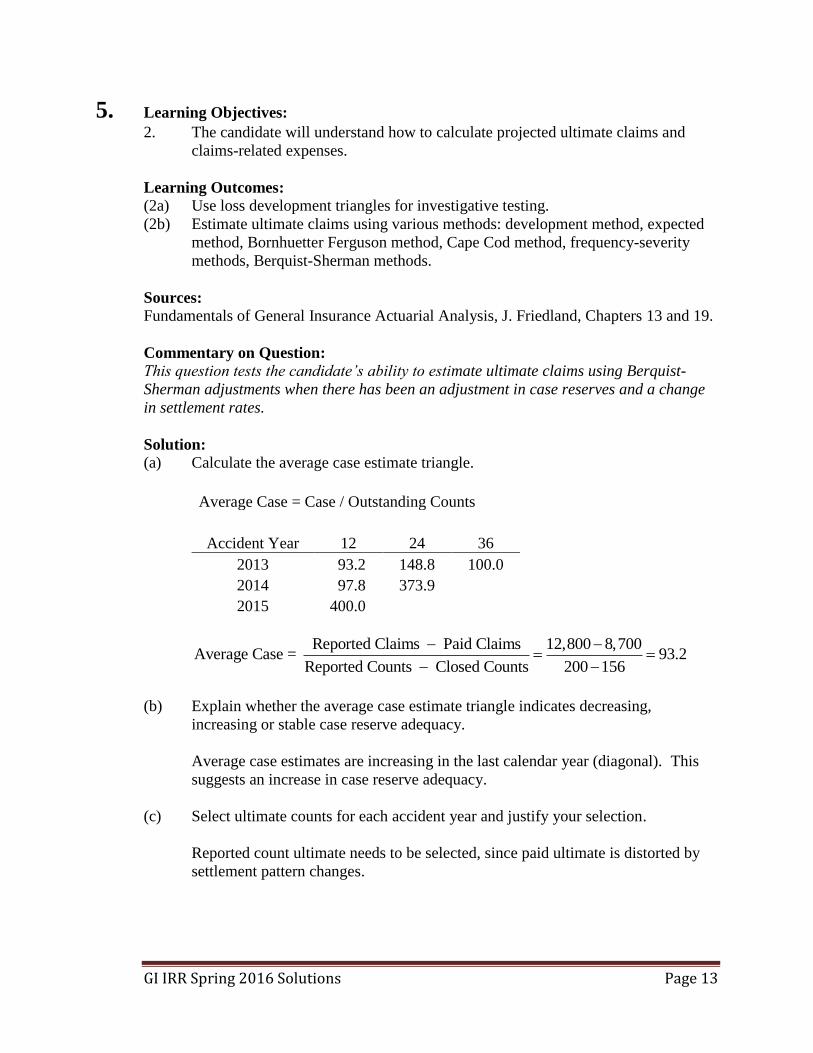
(a) Calculate the average case estimate triangle.

Average Case = Case / Outstanding Counts

Accident Year 12 24 36

2013 93.2 148.8 100.0

2014 97.8 373.9

2015 400.0

Reported Claims Paid Claims 12,800 8,700Average Case = 93.2

Reported Counts Closed Counts 200 156

(b) Explain whether the average case estimate triangle indicates decreasing,

increasing or stable case reserve adequacy.

Average case estimates are increasing in the last calendar year (diagonal). This

suggests an increase in case reserve adequacy.

(c) Select ultimate counts for each accident year and justify your selection.

Reported count ultimate needs to be selected, since paid ultimate is distorted by

settlement pattern changes.


5. Continued

(d) Calculate the disposal ratio triangle using the selections from part (c).

Disposal ratios = Closed Counts / Ultimate Counts


2013 0.520 0.697 0.933

2014 0.519 0.758

2015 0.613

e.g., 0.520 = 156 / 300

(e) Explain whether the disposal ratio triangle indicates decreasing, increasing or

stable claim settlement rates.

Disposal ratios are higher in last calendar year (diagonal), suggesting increasing

settlement rates, consistent with claims manager report of faster settlement of

small claims.

(f) Calculate the adjusted paid claims triangle.

12 24 36

Selected Disposal 0.6132 0.7581 0.9333

Adjusted Closed Counts = Disposal Ratio × Ultimate Reported


2013 184 227 280

2014 190 235

2015 195

Paid to Closed Ratio

AY13-15 55 50 68

Adjusted Paid = Adjusted Closed Counts × Paid to Closed Ratio


2013 10,120 11,350 19,040

2014 10,450 11,750

2015 10,725


5. Continued

(g) Calculate the adjusted reported claims triangle.

Adjusted Average Case = Selected Case (diagonal) detrended at 3%


2013 377.0 363.0 100.0

2014 388.3 373.9

2015 400.0

e.g., 388.3 = 400 / 1.03

Adjusted Open Counts = Reported Counts – Adjusted Closed


2013 16 23 20

2014 16 23

2015 17

Adjusted Case = Adjusted Average Case × Adjusted Open Counts


2013 6,032 8,349 2,000

2014 6,213 8,600

2015 6,800

Adjusted Reported = Adjusted Paid + Adjusted Case


2013 16,152 19,699 21,040

2014 16,663 20,350

2015 17,525


6. Learning Objectives: 5. The candidate will understand how to apply the fundamental ratemaking

techniques of general insurance.

Learning Outcomes:

(5d) Calculate loadings for catastrophes and large claims.

Sources:



This question tests the candidate’s understanding of claim loadings for ratemaking.

Solution:

(a) Describe four considerations for your assessment.

Any four of the following are acceptable:

The actuary should consider comparing historical insurance data to

noninsurance data to determine the extent to which the available historical

insurance data are fully representative of the long-term frequency and severity

of the perils.

The actuary should consider the sensitivity of the provision to changes in the

historical insurance data relating to the following: (1) the frequency of

catastrophes; (2) the severity of catastrophes; and (3) the geographic location

of catastrophes.

The actuary should consider the applicability of historical insurance data for

the insured coverage.

This includes determining:

o whether catastrophe losses are likely to differ significantly among

elements of the rate structure, such as construction type and location;

o whether such differences should be reflected in the ratemaking

procedures; and

o how to reflect such differences, taking into account both homogeneity and

the volume of data.

The actuary should consider whether there is a sufficient number of years of

comparable, compatible historical insurance data.


6. Continued

(b) Calculate the hail catastrophe loading as a claim ratio for annual policies starting

on April 1, 2016.

(1) (2)

Accident

Year

Earned

House

Years

Trended Hail

Ultimate Claims

(000)

2010 13,929 0

2011 14,070 0

2012 14,212 234

2013 14,356 0

2014 14,169 358

Total 70,736 592

(3) Trended Pure Premium for Hail Claims: (2) × 1000 / (1) = 8.37

(4) CY2014 Earned House Years: 14,169

(5) Hail Expected Claims: (3)(4) = 118,595

(6) CY2014 Trended Earned Premiums at Current Level: 11,291,000

(7) Catastrophe Claim Hail Loading Expressed as a Claim Ratio: (5)/(6) = 1.05%

(c) Describe two concerns you would have in relying on the calculation from part (b)

in your rating analysis.

Any two of the following are acceptable:

Frequency in the area not used

Severity in the area not used

No consideration of frequency trending

No consideration of the number of years used

No credibility

No formal cat modeling used

Change in exposure


6. Continued

(d) Recommend one improvement to address each concern identified in part (c).


The improvement must match the concern from part (c).

Frequency in the area not used compare frequency with a larger area

Severity in the area not used compare severity with the industry data

No consideration of frequency trending frequency seems too low to be

credible but should check

No consideration of the number of years used more potential data from

the industry

No credibility results should be credibility weighted

No formal cat modeling used use cat model

Change in exposure use simulation model or logic tree




Learning Outcomes:

(5j) Perform individual risk rating using standard plans.

Sources:



This question tests individual risk rating.

Solution:

(a) Identify two items of information to request in order to get a broader perspective

on the three companies and their historical experience.

Any two of the following are acceptable (other items are possible):

What was the premium for each year?

Explain the claim pattern in the experience period.

Provide individual claim data.

(b) Evaluate each company for retrospective rating, from the perspective of IRIE.

ABC:

Claims are relatively stable.

If claims can be controlled at level of 0.6, there could be an opportunity for

savings.

DEF:

Claims are relatively stable.

If claims continue at 0.8, there could be additional cost.

GHI:

Claims are not very stable.

Could there be a claim limitation if a large claim year like 2013 were to

reoccur?


7. Continued

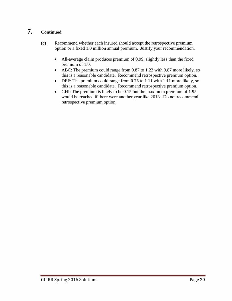
(c) Recommend whether each insured should accept the retrospective premium

option or a fixed 1.0 million annual premium. Justify your recommendation.

All-average claim produces premium of 0.99, slightly less than the fixed

premium of 1.0.

ABC: The premium could range from 0.87 to 1.23 with 0.87 more likely, so

this is a reasonable candidate. Recommend retrospective premium option.

DEF: The premium could range from 0.75 to 1.11 with 1.11 more likely, so

this is a reasonable candidate. Recommend retrospective premium option.

GHI: The premium is likely to be 0.15 but the maximum premium of 1.95

would be reached if there were another year like 2013. Do not recommend

retrospective premium option.




Learning Outcomes:

(5h) Calculate deductible factors, increased limits factors, and coinsurance penalties.

Sources:



This question tests the candidate’s understanding of and application of increased limit

factors and deductibles.

Solution:

(a) Calculate the observed increased limit factors (ILF) for:

(i) 250,000 limit

(ii) 500,000 limit

(iii) 1,000,000 limit

Limited Average Severity (LAS) @ 100,000 = [375,000 + 100 × (2,000+500)]/

(15,000+2,000+500) = 35.71

LAS @ 250,000 = [375,000 + 300,000 + (250 × 500)]/(15,000+2,000+500) =

45.71

LAS @ 500,000 = LAS @ 1,000,000 = [375,000 + 300,000 + 175,000]/

(15,000+2,000+500) = 48.57

ILF 100,000 to 250,000: 45.71/35.71 = 1.28

ILF 100,000 to 500,000: 48.57/35.71 = 1.36

ILF 100,000 to 1,000,000: 48.57/35.71 = 1.36

(b) Explain whether or not your selected ILF at 1,000,000 should equal your selected

ILF at 500,000.

Even though there are no claims in the 500,000 to 1,000,000 layer, this does not

mean the ILF should be the same.


8. Continued

(c) Describe two challenges insurers face when determining ILFs for high limits

using empirical data.

Answers could include any of the below:

Absence of complete data – insurers may not maintain ground-up uncapped

data on individual claims.

Claim development – an ultimate loss may reach a high limit, but not before it

is fully developed.

Claim trend – empirical claim data must be adjusted for trends, which will

influence the amount of claims at higher limits.

Empirical data at high limits often lacks credibility due to low frequency of

large losses.

(d) Calculate the amount of a covered loss retained by the insured and paid by the

insurer for the following covered losses:

Covered Loss

Retained by the

Insured Paid by the Insurer

900 900 0

1,400 600 800

2,000 0 2,000

e.g., for a covered loss of 1,400:

Paid by insurer = (1,400 – 1,000)×2 = 800

Paid by insured = 1,400 – 800 = 600

(e) Explain why increasing deductible amounts will reduce claim frequency, but will

not necessarily reduce the insurer’s claim severity.

An insurer is not responsible for paying claims below the deductible. As the

deductible increases, the insurer will pay fewer claims, which will reduce

frequency.

However, because increasing deductible amounts will lower both claim counts

and amounts, the insurer’s severity may increase when small claims are no longer

covered. This may lead to an increase in the average amount paid per claim, or a

higher severity.


9. Learning Objectives: 3. The candidate will understand financial reporting of claim liabilities and premium

liabilities.

Learning Outcomes:

(3e) Describe the components of premium liabilities in the context of financial

reporting.

Sources:



This question tests the determination of premium liabilities.

Solution:

(a) Calculate the 2016 pure premium per policy, gross and net of reinsurance.

(1) (2) (3) = (1)(2) (4) = (1)[1–0.25] (5) = min[(4),500] (6) = (2)(5)

Gross

Claim Per

Policy Probability

Gross Pure

Premium

Claim After

Quota Share

Claim After

Excess Reins

Net Pure

Premium

0 56% 0 0 0 0.00

100 30% 30 75 75 22.50

500 10% 50 375 375 37.50

2,000 4% 80 1,500 500 20.00

160 80.00

(b) Calculate the premium liabilities as of December 31, 2015, gross and net of

reinsurance.

Gross Net

(1) Average claim cost/year [from part (a)] 160 80

(2) Policies exposed for 2015 [50,000×50%] 25,000 25,000

(3) Expected Claim Cost [(1)(2)] 4,000,000 2,000,000

(4) ULAE [4,000,000×10%] 400,000 400,000

(5) Additional reinsurance cost [50×25,000] 1,250,000

(6) General expenses [3,750,000×20%×25%] 187,500 187,500

(7) Premium liabilities [(3)+(4)+(5)+(6)] 4,587,500 3,837,500

Note: (2) Average written date is July 1, 2015, therefore 50% exposed in 2015.


9. Continued

(c) Determine either the premium deficiency reserve or the equity in the unearned

premium.

Premium deficiency reserve = 3,837,500 – 3,750,000 = 87,500.

(d) State the maximum deferred policy acquisition expense (DPAE) ABC Insurance

could record as an asset.

Maximum DPAE = 0 (lower of the gross equity in the unearned premium and the

net equity in the unearned premium plus the ceded unearned commissions).




Learning Outcomes:




Sources:



This question tests the estimation of Allocated Loss Adjustment Expenses (ALAE) using

the development method and the expected method.

Solution:

(a) Identify one practical consideration in your decision .

Either of the following are acceptable:

The reporting and payment patterns are similar for indemnity and ALAE.

Differences in the reporting and payments of indemnity and ALAE are

consistent from year to year and consistent in the relationship of one to

another.

(b) Identify one situation where you should project indemnity and ALAE separately.

Either of the following are acceptable:

Where the insurer's practices for setting case estimates differ.

IT systems considerations, i.e., the insurer separates case estimates between

indemnity and ALAE.


10. Continued

(c) Calculate the ratio of ALAE to claims for each report year.

(1) (2) (3) = (1)/(2)

Report Year

Projected Ultimate

ALAE Based on

Reported Development

Method

Selected

Ultimate

Claims Ratio

2012 720 15,000 0.048

2013 740 16,100 0.046

2014 930 16,000 0.058

2015 820 16,400 0.050

Total 3,210 63,500 0.051

(d) Select an expected ratio of ALAE to claims. Justify your selection.

2014 seems to be an outlier.

Average of 2012, 2013, 2015 = 4.8%.

Select 4.8% as a reasonable estimate.

(e) Calculate the projected ultimate ALAE by report year using the expected ratio

from part (d).

(2) (4) = (2)×0.048

Report

Year

Projected Ultimate Claims

Based on Reported

Expected ALAE

Based on Ratio

2012 15,000 720

2013 16,100 773

2014 16,000 768

2015 16,400 787

Total 63,500 3,048


10. Continued

(f) Calculate the indicated ALAE IBNR by report year using the projected ultimate

ALAE from part (e).

(4) = (2)×0.048 (5) (6) = (4) – (5)

Report

Year

Expected ALAE

Based on Ratio

Reported ALAE

at Dec. 31, 2015

Expected Method

Indicated IBNR

2012 720 655 65

2013 773 630 143

2014 768 735 33

2015 787 570 217

Total 3,048 2,590 458

(g) Select the ALAE IBNR by comparing the indicated ALAE IBNR calculated in

part (f) with the indicated ALAE IBNR from the reported development method.

Justify your selection.

(1) (5) (6) = (4) – (5) (7) = (1) – (5)

Report

Year

Projected

Ultimate

Reported

ALAE

Reported ALAE

at Dec. 31, 2015

Expected

Method

Indicated

IBNR

Development

Method

Indicated

IBNR

2012 720 655 65 65

2013 740 630 143 110

2014 930 735 33 195

2015 820 570 217 250

Total 3,210 2,590 458 620

Candidates could recommend either of two options (the key is the justification for

the selection):

Option 1: IBNR for 2014 is too low using the expected method so select

development method IBNR of 195.

Report

Year

Selected

IBNR

2012 65

2013 143

2014 195

2015 217

Total 620


10. Continued

Option 2: The IBNR for 2014 using the expected method is reasonable, even if it

is a little low. The question says that there is uncertainty in the development

method so it is reasonable to use the expected method.

Report

Year

Selected

IBNR

2012 65

2013 143

2014 33

2015 217

Total 458




(5g) Calculate risk classification changes and territorial changes.

Sources:



This question tests the candidate’s understanding of risk classification.

Solution:

(a) Describe how a more refined risk classification system might lead to a

competitive advantage for a company.

An insurer with more refined pricing can charge a rate that is more closely related

to expected claims, attracting customers with a low risk of claims. Conversely, an

insurer with less refined pricing will encourage adverse selection; higher risk

customers will be attracted to the company.

(b) Calculate age one-way relativities and gender one-way relativities.

Overall average pure premium:

(90×200 + 100×125 + 80×150 + 110×120)/(90+100+80+110) = 146.58

One-way relativities for age:

Young: [(90×200 + 80×150)/(90+80)]/146.58 = 1.20

Old: [(100×125 + 110×120)/(100+110)]/146.58 = 0.83

One-way relativities for gender:

Male: [(90×200 + 100×125)/(90+100)]/146.58 = 1.10

Female: [(80×150 + 110×120)/(80+110)]/146.58 = 0.90

(c) Calculate indicated pure premiums for each age and gender combination without

rebalancing.

Young Male = 146.58 × 1.20 × 1.10 = 193.49

Old Male = 146.58 × 0.83 × 1.10 = 133.83

Young Female = 146.58 × 1.20 × 0.90 = 158.31

Old Male = 146.58 × 0.83 × 0.90 = 109.50


11. Continued

(d) Explain why one-way analysis fails to replicate the observed pure premiums in

this scenario.

Distributional bias and dependence cause the one-way relativities to produce

different pure premiums than observed.

(e) Calculate the revised pure premiums.

Young = 146.58 × 1.20 = 175.90

Old = 146.58 × 0.83 = 121.66

(f) Describe the potential rating effects on male and female policyholders.

Restrictions on using gender as a rating variable would result in females being

charged a rate higher than their relative risk and males being charged a rate lower

than their relative risk.




Learning Outcomes:

(2a) Use loss development triangles for investigative testing.




Sources:



This question tests the investigation of reported count triangles as well as estimating

ultimate counts using the development method.

Solution:

(a) Calculate the ultimate claim counts for each accident year using the development

method with a simple all-year average and a tail factor of 1.05.

Accident Year 12-24 24-36 36-48 48-Ult

2012 3.700 1.369 1.135

2013 3.724 1.403

2014 4.398

Simple average 3.941 1.386 1.135 1.050

Age-to-Ultimate 6.510 1.652 1.192 1.050

e.g., 3.700 = 1,850 / 500

(1) (2) (3) = (1)(2)

Accident

Year

Reported

Counts at

Dec. 31, 2015

Age-to-Ultimate

Development

Factors

Ultimate

Counts

2012 2,875 1.050 3,019

2013 3,030 1.192 3,612

2014 2,243 1.652 3,705

2015 515 6.510 3,353

Total 13,689

(b) Identify one item to investigate based on the reported count triangle and the

development factors calculated in part (a).

2014 12-24 development factor is higher than 2012 and 2013.


12. Continued

(c) Describe how you would investigate the item identified in part (b).

One could approach the claims department to see if there has been a process

change in the speed of settling claims.

(d) Identify three reasons a reinsurer’s experience may be more variable than the

primary insurer’s experience.

Any three of the following are acceptable (other answers are possible):

Reinsurer typically covers higher layer which has more uncertainty.

Reinsurer will have less data so lower credibility.

There are often lengthy lags in reporting experienced by reinsurers.

Random deviations in reported claims will have a magnified effect because

the projected ultimate values are highly dependent on reported claims.




Learning Outcomes:




Sources:



This question tests the frequency-severity closure method of estimating ultimate claims.

Solution:

(a) Describe a data adjustment to use with the closure method if the line of business

has a significant number of partial payments.

The closed count triangle should ideally be matched with a triangle of paid claims

on closed counts.

(b) Calculate the proportion of closed counts at each maturity age for accident year

2012.

First calculate the incremental closed counts at each maturity age for 2012:

12: 9,670

24: 12,120 – 9,670 = 2,450

36: 12,980 – 12,120 = 860

48: 13,380 – 12,980 = 400

Next, at each maturity age, the proportion of closed counts is equal to the

incremental counts closed divided by the counts not yet closed.

12: 9,670 / 13,380 = 0.723

24: 2,450 / (13,380 – 9,670) = 0.660

36: 860 / (13,380 – 12,120) = 0.683

48: 400 / (13,380 – 12,980) = 1.000


13. Continued

(c) Calculate the incremental closed counts for accident year 2014 at all maturities 12

through 48 months.

The incremental closed count for age 12 is given as 5,960.

The incremental closed count for age 24 is 7,420 – 5,960 = 1,460.

For the remaining ages, it is equal to (the ultimate count minus the cumulative

closed count) × selected proportion of closed counts:

36: (8,500 – 7,420) × 0.70 = 756

48: (8,500 – 7,420 – 756) × 1.000 = 324

(d) Calculate the incremental paid severity for accident year 2014 at all maturities 12

through 48 months.

The incremental paid severity for ages 12 and 24 are as shown in the table

provided: 1,175 for age 12 and 4,200 for age 24.

For the remaining ages, it is simply the selected severity adjusted for the

cumulative trend of 1.035 from 2015 to 2014:

36: 12,800 / 1.035 = 12,367

48: 14,500 / 1.035 = 14,010

(e) Calculate the accident year 2014 projected ultimate claims.

Incremental paid claims are equal to the incremental closed counts from part (c)

multiplied by the corresponding incremental severities from part (d). Thus:

12: 5,960 × 1,175 = 7,003,000

24: 1,460 × 4,200 = 6,132,000

36: 756 × 12,367 = 9,349,452

48: 324 × 14,010 = 4,539,240

Total = 7,003,000 + 6,132,000 + 9,349,452 + 4,539,240 = 27,023,692




Learning Outcomes:




Sources:



This question tests the candidate’s understanding (calculation and purpose) of the Cape

Cod method and the Generalized Cape Cod method.

Solution:

(a) Calculate the used-up on-level earned premiums for each accident year.

On-level Calculation:

Rate

Level

Rate Level

Relative Value

% Earned in CY

2013 2014 2015

A 1.00 100.0% 87.5% 12.5%

B 0.94 0.0% 12.5% 87.5%

Average rate level 1.0000 0.9925 0.9475

On-level factor 0.948 0.955 1.000

(relative to 2015 average rate level)

2013 2014 2015

A

B

6% rate decrease July 1, 2014


14. Continued

(1) (2) (3) = (1)(2) (4) (5) = 1/(4) (6) = (3)(5)

Accident

Year

Earned

Premium

Premium

On-Level

Factor

On-Level

Earned

Premium

Reported

CDF

Expected %

Reported

Used-Up

On-Level

Earned

Premium

2013 40,000 0.948 37,900 1.250 0.80 30,320

2014 41,000 0.955 39,141 2.000 0.50 19,571

2015 40,000 1.000 40,000 5.000 0.20 8,000

Total 57,891

(b) Calculate the expected claims for each accident year.

(7) (8) (9) (10)=(7)(8)(9) (11) = 0.694×(3)/[(8)(9)]

Accident

Year

Actual

Reported

Claims

Trend

Factor

Tort

Reform

Adjusted

Claims Expected Claims

2013 22,000 1.040 0.900 20,600 28,083

2014 14,000 1.020 0.950 13,566 28,026

2015 6,000 1.000 1.000 6,000 27,753

Total 40,166 83,862

Notes: Trend factor = 1.02(2015–AY)

Adjusted expected claim ratio = 40,166 / 57,891 = 0.694

(c) Calculate the estimated ultimate claims for each accident year.

(7) (12) = 1 – (5) (13) = (11)(12) (14) = (7) + (13)

Accident

Year

Actual

Reported

Claims

Expected %

Unreported

Expected

Unreported

Projected

Ultimate

2013 22,000 0.20 5,617 27,617

2014 14,000 0.50 14,013 28,013

2015 6,000 0.80 22,202 28,202

Total 41,832 83,832


14. Continued

(d) Explain why the Cape Cod method may not be appropriate for coverages such as

property or collision.

Development factor may be less than 1.0 which will result in used-up exposures

that are greater than the original exposures.

(e) Explain the purpose of a decay factor.

The decay factor allows different weighting of the years in the experience period

with the greatest weight being applied to the year under consideration (origin

year) and then decreasing weights to the years preceding and subsequent to the

origin year. The decay factor is judgmentally selected between 0% and 100%.

(f) Identify the methods that the Generalized Cape Cod method approaches when the

decay factor approaches zero and approaches one.

When decay factor = 0, the Generalized Cape Cod method returns the

development method result.

When decay factor = 1, the Generalized Cape Cod method returns the traditional

Cape Cod method result.


14. Continued

(g) Calculate the expected claims for accident year 2015 using the Generalized Cape

Cod method with a decay factor of 70%.

(1) (6) (10) (15) (16) (17) = (1)(16)

Accident

Year

Earned

Premium

Used-Up

On-Level

Earned

Premium

Adjusted

Claims

70%

Decay

Factors

Expected

Claim Ratio

Expected

Claims

2013 40,000 30,320 20,600 49%

2014 41,000 19,571 13,566 70%

2015 40,000 8,000 6,000 100% 0.700 28,000

57,891 40,166

Notes: Expected claim ratio (16) = sumproduct[(10),(15)] / sumproduct[(6),(15)]

Expected claims (17) = (1)(16) = 40,000×0.700




Learning Outcomes:

(2d) Explain the effect of changing conditions on the projection methods cited in (2b).

Sources:



This question tests the candidate’s understanding of changing conditions on data,

assumptions, and methods.

Solution:

(a) Explain the likely row, column, or diagonal effects each event had on the data.


(i) Expect higher claim ratios in AY 2012 and subsequent (multiple rows).

(ii) Expect a temporary slowdown (decrease) in reported claim activity on

accident year (AY) 2013 which means the reported claims (frequency)

evaluated at 12 months could be low. However, cumulative patterns will

self-correct by 24 months.

There could also be a temporary slowdown (decrease) in paid or closed

activity on other AYs in the calendar year (CY) 2013 diagonal. This

slowdown (decrease) should be offset by an increase in the next CY

diagonal (2014).

(iii) Expect claims to increase for CYs 2010 and subsequent (CY effect) (i.e.,

all open claims are affected).

(b) Explain how you would handle each event through a data adjustment, assumption,

or method selection.


(i) Development on AYs 2012 and subsequent should be given higher weight

in making age-to-age development factor selections on AYs 2012 and

subsequent.


15. Continued

(ii) Since we are now evaluating experience as of Dec 31, 2015, this anomaly

should not be an issue in estimating AY 2013 claims. AY 2013 12-24

month development factor (or the entire row) should be excluded from

future analyses.

(iii) Development factors from CYs 2010 and subsequent should be given

higher weight in making age-to-age development factor selections on all

AYs.

(c) Describe one situation (different from those above) that might lead you to use a

Berquist-Sherman adjustment in estimating ultimate claim ratios for auto liability

business.


A change in claim department settlement patterns.


16. Learning Objectives: 7. The candidate will understand the nature and application of catastrophe models

used to manage risks from natural disasters.

Learning Outcomes:

(7b) Apply catastrophe models to insurance ratemaking, portfolio management, and

risk financing.

Sources:

Catastrophe Modeling: A New Approach to Managing Risk, Grossi, P. and Kunreuther,

H., Chapter 6.

Solution:

(a) Rank the following portfolios from least to most catastrophe risk from GIC’s

perspective, with the possibility that some may be roughly equal in risk. Justify

your ranking.

I. ABC only

II. FGH only

III. XYZ only

IV. ABC and FGH

V. ABC and XYZ

VI. FGH and XYZ

VII. ABC, FGH, and XYZ

Commentary on Question: Candidates generally did poorly, failing to understand that combining portfolios

brings diversification and thus reduces risk. Alternative answers could earn full

credit. For example, ABC and XYZ could be ranked with one riskier than the

other. This is acceptable provided a reasonable explanation was provided.

Another alternative is to have so little risk associated with FGH that any portfolio

that includes it will be viewed as less risky than those that do not.

For the individual portfolios, FGH is less risky than ABC and XYZ, which are

about equal. That is because tornados cause less widespread damage (and hence

are not discussed in the text). The other consideration is that combining any of

these portfolios provides diversification and thus a reduction in overall riskiness.

This leads to a ranking of

VII < IV = VI < V < II < I = III.

(b) Describe an action GIC may take to improve its underwriting to account for

ABC’s earthquake risk.

GIC could obtain detailed underwriting information about each property, perhaps

including inspection by an engineer.


16. Continued

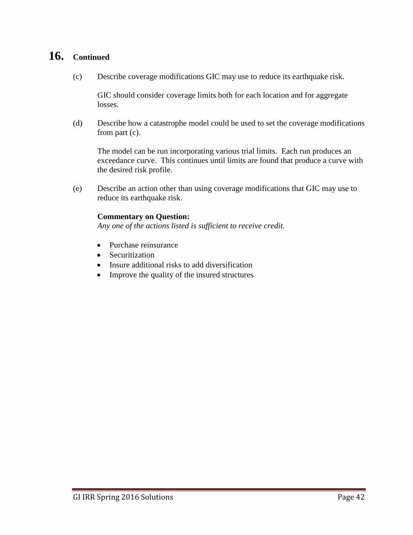
(c) Describe coverage modifications GIC may use to reduce its earthquake risk.

GIC should consider coverage limits both for each location and for aggregate

losses.

(d) Describe how a catastrophe model could be used to set the coverage modifications

from part (c).

The model can be run incorporating various trial limits. Each run produces an

exceedance curve. This continues until limits are found that produce a curve with

the desired risk profile.

(e) Describe an action other than using coverage modifications that GIC may use to

reduce its earthquake risk.

Commentary on Question: Any one of the actions listed is sufficient to receive credit.

Purchase reinsurance

Securitization

Insure additional risks to add diversification

Improve the quality of the insured structures




Learning Outcomes:

(5j) Perform individual risk rating using standard plans.

(5k) Calculate rates for claims-made coverage.

Sources:



This question tests individual risk rating and claims-made ratemaking.

Solution:

(a) Provide two advantages of claims-made and two advantages of occurrence

coverage for ERR.

Two advantages of claims-made:

less uncertainty in pricing

less effect due to sudden changes in either the trend or the reporting pattern

Two advantages of occurrence coverage:

greater opportunity for investment income

less risk of coverage gaps

(b) Identify three risk characteristics that can be used in schedule rating for the group.

Any three of the following are acceptable (other characteristics are possible):

risk management program

geographical scope of practice

range of assignments

experience

peer review

(c) Provide a reason why the total allowable schedule rating credits or debits for all

risk characteristics combined is generally limited.

Schedule credits and debits generally have a limit due to either regulatory rules

and regulations or internal company policies.


17. Continued

(d) Assess the credibility of the historical data from ERR.

For a long experience period of ten years, there are only 100 claims. Even

assuming a credibility standard of 400 claims and the square root rule, ERR's

experience is only partially credible ( 100 / 400 0.5 ).

(e) Calculate the step factors from first-year through maturity for the following cases:

(i) Claims-made

(ii) Claims-paid


An amount of 10 per year is used as an illustrative example.

Claims-Made Reporting Pattern Claims-Paid Payment Pattern

Report Year Report Year

AY Lag 1 2 3 4 AY Lag 1 2 3 4 5

0 10 0 5

1 10 10 1 10 10

2 10 10 10 2 10 10 10

3 10 10 10 10 3 10 10 10 10

Total 40 60 4 5 5 5 5 5

Total 40 80

(i) Claims-made step factors:

10/40 = 0.25

20/40 = 0.50

30/40 = 0.75

40/40 = 1.00

(ii) Claims-paid step factors:

5/40 = 0.125

15/40 = 0.375

25/40 = 0.625

35/40 = 0.875

40/40 = 1.000


17. Continued

(f) (1 point) Calculate the tail factor applicable to a mature policy for the following

cases:

(i) Claims-made

(ii) Claims-paid

(i) Claims-made tail factor = 60/40 = 1.5

(ii) Claims-paid tail factor = 80/40 = 2.0




Learning Outcomes:

(4d) Describe the influences on exposures and premiums of changes in deductibles,

changes in policy limits, and changes in mix of business.

(4e) Choose trend rates and calculate trend factors for exposures.

Sources:



This question tests the candidate’s understanding of premium trend analysis, particularly

when the trend rate changes.

Solution:

(a) Explain one reason not to use actual premium when analyzing premium trend.

Using actual (unadjusted) premiums could result in trend estimates that reflect

rate changes and not an underlying trend.

(b) Calculate the 2010 premium trend factor.

Commentary on Question: Candidates had difficulty setting the dates to which the two trend factors are

applied.

Policies written between January 1, 2009 and December 31, 2010 contribute

toward 2010 earned premiums. The average written date is thus January 1, 2010.

The first trending period is from January 1, 2010 to January 1, 2012, which is 2

years. The total trend is 1.022 = 1.0404.

The rates will be in effect for one year starting September 1, 2016. The average

written date in the forecast period is six months later, or March 1, 2017. Thus, the

second trending period is from January 1, 2012 to March 1, 2017, which is 5 1/6

years. The trend for this period is 1.00755.167 = 1.0394.

The 2010 premium trend factor is 1.0404 × 1.0394 = 1.0814.


18. Continued

(c) Describe what would have been different in the calculation if the work done in

part (b) was for a self-insurer.

The difference is that a self-insurer is essentially a single policy, not a series of

policies written over the period. Therefore, the average written dates would

reflect the actual date the policy is written.

(d) Explain how the premium trend factors would be affected by the following:.

(i) An increasing proportion of insureds choosing a higher policy limit at the

beginning of 2014

(ii) An increasing proportion of insureds choosing a higher deductible at the

beginning of 2014

(i) The increased policy limit would increase the premiums and thus the

premium trend factor would increase.

(ii) The higher deductible would decrease the premiums and thus the premium

trend factor would decrease.




5. The candidate will understand how to apply the fundamental ratemaking


Learning Outcomes:

(4c) Choose trend rates and calculate trend factors for claims.

(5b) Calculate expenses used in ratemaking analyses including expense trending

procedures.

(5f) Calculate overall rate change indications under the claims ratio and pure premium

methods.

Sources:

Fundamentals of General Insurance Actuarial Analysis, J. Friedland, Chapters 25, 29, and

31.


This question tests expense loadings and basic ratemaking.

Solution:

(a) Calculate the weighted average trended pure premium.

(1) (2) (3) (4) (5) (6)

Average Earned Date

Accident

Year

Earned

Exposures

Ultimate

Claims Exposure Experience

Trending

Period

Trended

Ultimate PP

2013 5,100 2,082,000 7/1/2013 10/1/2017 4.25 444.08

2014 5,250 2,250,000 7/1/2014 10/1/2017 3.25 457.06

2015 5,200 2,178,000 7/1/2015 10/1/2017 2.25 437.93

Weighted average trended pure premium 444.90

Notes: (6) = (2)(1.02)(5)/(1)

(6)Total = 0.2×444.08 + 0.3×457.06 + 0.5×437.93 = 444.90


19. Continued

(b) Recommend how you would include a provision for the health levy in your

ratemaking analysis. Justify your recommendation.


Either option is acceptable. The key is the justification for the approach.

Option 1: Recommend using a percentage of premium approach. The justification

is that higher premium drivers are higher risks and therefore should pay more

toward the health levy.

Option 2: Recommend using a flat fee per policy (exposure). The justification is

that every risk should pay an equal amount toward the levy.

(c) Calculate the provision for the health levy to include in your ratemaking analysis.

Either method is acceptable.

Option 1 (percentage): 119,000 / 2,761,000 = 4.31% (assumes the levy in rating

period will continue to be the same ratio to premium so no trending required).

Option 2 (fixed expense):

Fixed expense = 119,000 / 5,200 = 22.88

Need to trend to future rating period (from 2015) = 2.25 years

Trended fixed expense for levy = 22.88×1.012.25 = 23.40

(d) Calculate the indicated rate.

Option 1 (levy as variable):

Total variable expense = 0.12 + 0.0431 = 0.1631

Indicated rate = ( (1 ) ) (445 1.05 20)

603.851 1 0.1631 0.03

PP ULAE F

V Q

Option 2 (levy as additional fixed expense):

Total F = 20 + 23.40 = 43.40

Indicated rate = ( (1 ) ) (445 1.05 43.40)

600.771 1 0.12 0.03

PP ULAE F

V Q


19. Continued

(e) Determine whether or not the target for profit and contingencies will be met based

on your indicated rate from part (d).

Use formula 31.11: P = C + (F × E) + (V × P) + (Q × P)

Solve for (1 ) ( )

1C ULAE F E

Q VP

Option 1: F×E = 20×5,400 = 108,000

V = 16.31%

2,450,000 (1.05) 108,000

1 16.31% 1.5%603.85 5,400

Q

Therefore, since Q < 3% target, target is not met.

Option 2: F×E = 43.40×5,400 = 234,360

V = 12%

2,450,000 (1.05) 234,360

1 12% 1.5%600.77 5,400

Q

Therefore, since Q < 3% target, target is not met.

giirr model solutions - soa.org model solutions spring 2016 1. ... the rate level relative value for...

Documents