gis floodplain mapping in d highway d fctr.utexas.edu/wp-content/uploads/pubs/1738_4.pdf · gis for...

RESEARCH REPORT 1738-4

GIS FOR FLOODPLAIN MAPPING IN

DESIGN OF HIGHWAY

DRAINAGE FACILITIES

David Maidment, Eric Tate, and Francisco Olivera

CENTER FOR TRANSPORTATION RESEARCHBUREAU OF ENGINEERING RESEARCHTHE UNIVERSITY OF TEXAS AT AUSTIN

A U G U S T 1 9 9 8

Technical Report Documentation Page

1. Report No.

FHWA/TX-99/1738-4

2. Government Accession No. 3. Recipient’s Catalog No.

5. Report Date

August 1998

4. Title and Subtitle

GIS FOR FLOODPLAIN MAPPING IN DESIGN

OF HIGHWAY DRAINAGE FACILITIES 6. Performing Organization Code

7. Author(s)


8. Performing Organization Report No.

1738-4

10. Work Unit No. (TRAIS)9. Performing Organization Name and Address

Center for Transportation ResearchThe University of Texas at Austin3208 Red River, Suite 200Austin, TX 78705-2650

11. Contract or Grant No.

0-1738

13. Type of Report and Period Covered

Research Report (9/97 – 8/98)

12. Sponsoring Agency Name and Address

Texas Department of TransportationResearch and Technology Transfer Section/Construction DivisionP.O. Box 5080Austin, TX 78763-5080

14. Sponsoring Agency Code

15. Supplementary Notes

Project conducted in cooperation with the Federal Highway Administration.

16. Abstract

Since the 1960s, civil engineers have employed a variety of computer models for stream floodplain analysis. HEC-2 and its Windows counterpart, HEC-RAS, have been the principal models used for such analyses. A significantdeficiency of these programs is that the location of structures impacted by floodwaters, such as roads, homes, andbusinesses, cannot be effectively compared to the floodplain location. This report presents straightforwardapproaches to processing HEC-RAS output to enable two- and three-dimensional floodplain mapping in ageographic information system (GIS). The methodology was applied to a segment of Waller Creek in Austin,Texas. The HEC-RAS stream geometry and flood elevation data were imported into ArcView GIS, in which thecross sections were mapped along a digital representation of the stream. A planimetric view of the floodplain wasdeveloped using a digital orthophotograph as a base map. An approach to three-dimensional floodplainvisualization through the integration of HEC-RAS stream cross-section data into a digital terrain model of the studyarea is under development. The results indicate that GIS is an effective environment for floodplain visualizationand analysis.

17. Key Words

Hydraulic modeling, HEC-RAS, GeographicInformation Systems, GIS, floodplain mapping

18. Distribution Statement

No restrictions. This document is available to the publicthrough the National Technical Information Service,Springfield, Virginia 22161.

19. Security Classif. (of report)

Unclassified

20. Security Classif. (of this page)

Unclassified

21. No. of pages

36

22. Price

Form DOT F 1700.7 (8-72) Reproduction of completed page authorized

GIS FOR FLOODPLAIN MAPPING IN DESIGN OF

HIGHWAY DRAINAGE FACILITIES

by


Research Report Number 1738-4

Research Project 0-1738

System of GIS-Based Hydrologic and Hydraulic

Applications for Highway Engineering

Conducted for the

TEXAS DEPARTMENT OF TRANSPORTATION

in cooperation with the

U.S. DEPARTMENT OF TRANSPORTATIONFederal Highway Administration

by the

CENTER FOR TRANSPORTATION RESEARCH

Bureau of Engineering Research

THE UNIVERSITY OF TEXAS AT AUSTIN

August 1998

iii

DISCLAIMERS

The contents of this report reflect the views of the authors, who are responsible forthe facts and the accuracy of the data presented herein. The contents do not necessarilyreflect the official views or policies of the Federal Highway Administration or the TexasDepartment of Transportation. This report does not constitute a standard, specification, orregulation.

There was no invention or discovery conceived or first actually reduced to practicein the course of or under this contract, including any art, method, process, machine,manufacture, design or composition of matter, or any new and useful improvement thereof,or any variety of plant, which is or may be patentable under the patent laws of the UnitedStates of America or any foreign country.

NOT INTENDED FOR CONSTRUCTION,BIDDING, OR PERMIT PURPOSES

David Maidment, P.E. (Texas No. 53819)Research Supervisor

ACKNOWLEDGMENTS

The authors acknowledge the support of TxDOT Project Director AnthonySchneider (DES) and former Project Director Peter Smith. Also appreciated is the assistanceprovided by T. D. Ellis (PAR).

�Research performed in cooperation with the Texas Department of Transportation and theU.S. Department of Transportation, Federal Highway Administration.

v

�TABLE OF CONTENTS�

CHAPTER 1. BACKGROUND ........................................................................................ 1

OPEN CHANNEL FLOW THEORY ..................................................................... 1

Flow Classification...................................................................................... 1

Flow and Conveyance ................................................................................. 2

Energy Equation.......................................................................................... 4

HEC-RAS ............................................................................................................... 5

HEC-RAS Parameters ................................................................................. 6

Water Surface Profile Computation ............................................................ 7

GEOGRAPHIC INFORMATION SYSTEMS........................................................ 8

PREVIOUS WORK ................................................................................................ 10

CHAPTER 2. METHODOLOGY...................................................................................... 13

DATA IMPORT FROM HEC-RAS........................................................................ 13

STREAM CENTERLINE DIGITAL REPRESENTATION................................... 16

CROSS-SECTION GEOREFERENCING.............................................................. 17

CHAPTER 3. PRELIMINARY RESULTS ....................................................................... 21

REFERENCES ................................................................................................................... 23

�

vi

�

vii

INTRODUCTION

Much of the cost of most highway projects is attributable to drainage facilities,

including storm drains, highway culverts, bridges, and water quality and quantity control

structures. Design of these facilities involves hydrologic analysis to determine the design

discharge and hydraulic analysis of the conveyance capacity of the facility. In this report, a

geographic information systems (GIS) approach for floodplain mapping to aid in the design

of drainage facilities is presented. The methodology was developed to reduce the analysis

time and to improve its accuracy by integrating spatial stream geometry with hydraulic

analysis. The Texas Department of Transportation (TxDOT) has existing procedures for

hydrologic and hydraulic analysis in the Texas Hydraulic System (THYSYS). Each

THYSYS application requires the computerization of the description of the watershed and

the stream channel using data extracted manually from maps and cross sections contained in

paper drawings. In developing a GIS approach for floodplain mapping, the extraction of

data and application of design procedures becomes more efficient.

In a relatively short time, GIS has gained widespread use in a variety of engineering

applications. Originally envisioned (and used) as a geographic mapper with integrated

spatial database, GIS is increasingly being used in modeling applications, where geographic

data can be readily accessed, processed, and displayed. Historically, GIS has been

implemented primarily by large entities, such as federal, state, and local government

agencies, predominantly for mapping and management of spatial data. However, there is

increasing interest in the potential application of GIS in engineering design and analysis,

especially in hydrology and hydraulics.

The principal objective of the hydraulic model research is to develop a procedure

that can take a set of computed water surface profiles and construct an associated GIS

floodplain map. The work consists of geographically referencing hydraulic modeling

output and forming an integrated terrain model combining data on the general landscape

with data for stream channel morphology. These tasks are described in detail in the

following chapters.

1

CHAPTER 1. BACKGROUND

This chapter introduces concepts and associated terminology that formed the

backbone of the work completed for this project. The discussion includes open channel

flow theory, the HEC-RAS hydraulic model, and GIS.

OPEN CHANNEL FLOW THEORY

Open channel flow is defined as the flow of a free surface fluid within a defined

channel. Typical examples include flow in natural streams, flow in constructed drainage

canals, and flow in storm sewers. The development of plans to effectively manage

floodplains requires that hydraulic engineers understand the hydraulics of open channel

flow, which depend on the flow classification, flow and conveyance, and the energy

equation.

Flow Classification

Open channel flow is classified based on changes in time, space, and flow regime:

�� Time. Steady flow describes conditions under which depth and velocity at a

specific channel location do not change with time. In contrast, unsteady flow

refers to flow conditions that change with time at a given location.

�

�� Space. The term uniform flow denotes fluid flow, in which depth and velocity

are constant with distance. Uniform flow conditions require the channel to be

straight, with constant cross-sectional geometry, and a water surface that is

parallel to the base of the channel. In varied flow, water depth and velocity

change with distance along the channel.

�

2

��

��

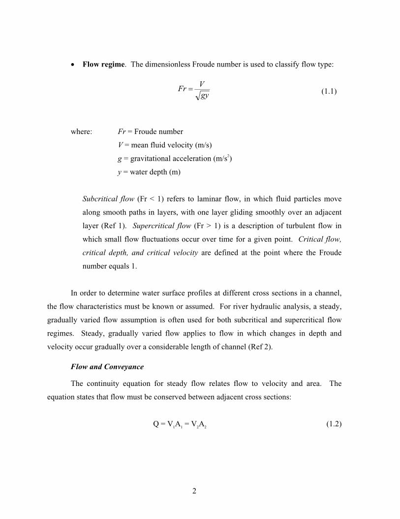
�� Flow regime. The dimensionless Froude number is used to classify flow type:

�

� (1.1)

�

�

�where: Fr = Froude number

� V = mean fluid velocity (m/s)

� g = gravitational acceleration (m/s2)

� y = water depth (m)

�

�Subcritical flow (Fr < 1) refers to laminar flow, in which fluid particles move

along smooth paths in layers, with one layer gliding smoothly over an adjacent

layer (Ref 1). Supercritical flow (Fr > 1) is a description of turbulent flow in

which small flow fluctuations occur over time for a given point. Critical flow,

critical depth, and critical velocity are defined at the point where the Froude

number equals 1.

�

In order to determine water surface profiles at different cross sections in a channel,

the flow characteristics must be known or assumed. For river hydraulic analysis, a steady,

gradually varied flow assumption is often used for both subcritical and supercritical flow

regimes. Steady, gradually varied flow applies to flow in which changes in depth and

velocity occur gradually over a considerable length of channel (Ref 2).

�Flow and Conveyance

�The continuity equation for steady flow relates flow to velocity and area. The

equation states that flow must be conserved between adjacent cross sections:

�

� Q = V1A1 = V2A2 (1.2)

3

��

��

��

�

��

��

��

��

�

�

��

��

��

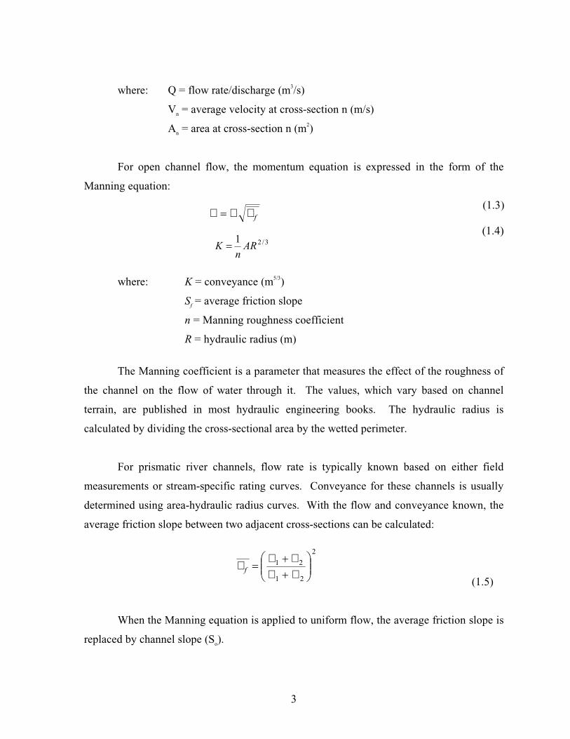
�where: Q = flow rate/discharge (m3/s)

�Vn = average velocity at cross-section n (m/s)

�An = area at cross-section n (m2)

�

�For open channel flow, the momentum equation is expressed in the form of the

Manning equation:

� (1.3)

� ��

�

�where: K = conveyance (m5/3)

�Sf = average friction slope

�n = Manning roughness coefficient

�R = hydraulic radius (m)

�

The Manning coefficient is a parameter that measures the effect of the roughness of

the channel on the flow of water through it. The values, which vary based on channel

terrain, are published in most hydraulic engineering books. The hydraulic radius is

calculated by dividing the cross-sectional area by the wetted perimeter.

For prismatic river channels, flow rate is typically known based on either field

measurements or stream-specific rating curves. Conveyance for these channels is usually

determined using area-hydraulic radius curves. With the flow and conveyance known, the

average friction slope between two adjacent cross-sections can be calculated:

�

(1.5)

�

�When the Manning equation is applied to uniform flow, the average friction slope is

replaced by channel slope (So).

4

�

��

�

��

��

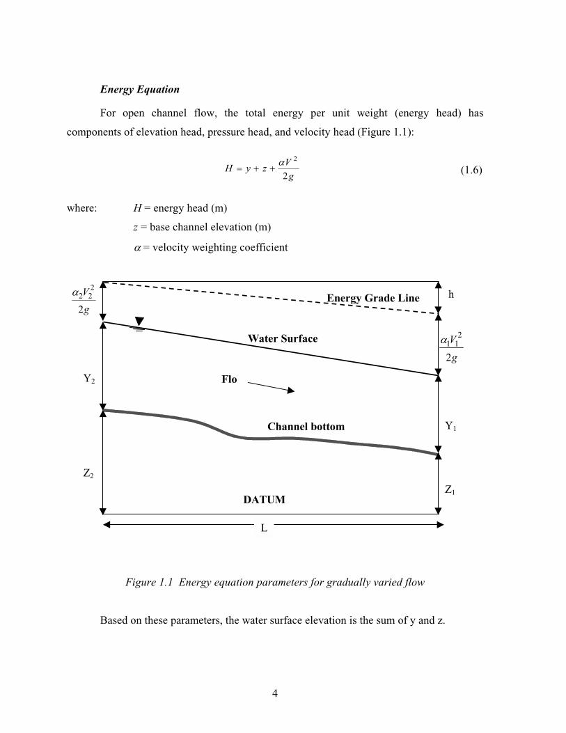
�Energy Equation

�For open channel flow, the total energy per unit weight (energy head) has

components of elevation head, pressure head, and velocity head (Figure 1.1):

�

� (1.6)

�

�where: H = energy head (m)

�z = base channel elevation (m)

�� = velocity weighting coefficient

�

�

�

�Figure 1.1 Energy equation parameters for gradually varied flow

�

�Based on these parameters, the water surface elevation is the sum of y and z.

�

�

�

�

��

��

��

�

�

�

�

��

��

��

�

��

��

��

��

��

5

��

��

��

�

�

�

��

��

�

�

�

� ��

��

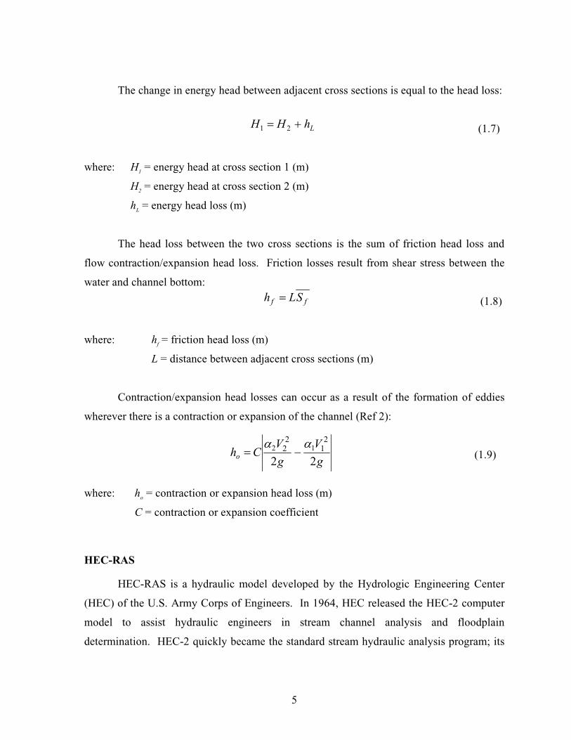
�The change in energy head between adjacent cross sections is equal to the head loss:

�

� (1.7)

�

�where: H1 = energy head at cross section 1 (m)

� H2 = energy head at cross section 2 (m)

� hL = energy head loss (m)

�

� The head loss between the two cross sections is the sum of friction head loss and

flow contraction/expansion head loss. Friction losses result from shear stress between the

water and channel bottom:

� (1.8)

�

�where: hf = friction head loss (m)

� L = distance between adjacent cross sections (m)

�

�Contraction/expansion head losses can occur as a result of the formation of eddies

wherever there is a contraction or expansion of the channel (Ref 2):

�

� (1.9)

�

�where: ho = contraction or expansion head loss (m)

� C = contraction or expansion coefficient

�

�HEC-RAS

HEC-RAS is a hydraulic model developed by the Hydrologic Engineering Center

(HEC) of the U.S. Army Corps of Engineers. In 1964, HEC released the HEC-2 computer

model to assist hydraulic engineers in stream channel analysis and floodplain

determination. HEC-2 quickly became the standard stream hydraulic analysis program; its

6

capabilities were expanded in the ensuing years to provide for, among other things, bridge,

weir, and culvert analysis. Although HEC-2 was originally developed for mainframe use, it

can currently operate on personal computers (in DOS mode) and on workstations (Ref 3).

In response to the increased use of Windows-based personal computing software, HEC

released in the early 1990s a Windows-compatible counterpart to HEC-2 called the River

Analysis System (RAS). HEC-RAS is intended for one-dimensional steady flow water

surface profile computations, unsteady flow simulation, and movable boundary sediment

transport calculations. The system is capable of modeling subcritical, supercritical, and

mixed-flow regimes for streams consisting of a full network of channels, a dendritic system,

or a single river reach. The model results are typically applied in floodplain management

and flood insurance studies to evaluate floodway encroachments (Ref 4).

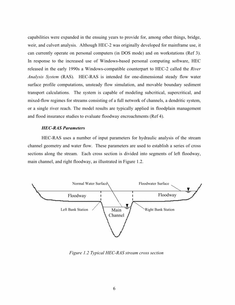
�HEC-RAS Parameters

�HEC-RAS uses a number of input parameters for hydraulic analysis of the stream

channel geometry and water flow. These parameters are used to establish a series of cross

sections along the stream. Each cross section is divided into segments of left floodway,

main channel, and right floodway, as illustrated in Figure 1.2.

�

�

�Figure 1.2 Typical HEC-RAS stream cross section

�

��

��

��

��

��

��

7

�At each cross section, several geometry parameters are required to describe shape,

elevation, and relative location along the stream:

�

�� River station (cross section) number

�� Lateral and elevation coordinates for each (dry, unflooded) terrain point

�� Left and right bank station locations

�� Reach lengths between the left floodway, main channel, and right floodway of

adjacent river stations (The three-reach lengths represent the average flow path

through each segment of the cross section pair. As such, the reach lengths

between adjacent cross sections may differ owing to bends in the stream.)

�� Manning’s roughness coefficients

�� Contraction and expansion coefficients

�� Geometric description of any hydraulic structures (bridges, culverts, weirs, etc.)

At each cross-section line, HEC-RAS assumes that energy is constant and that the

velocity vector is perpendicular. As such, care should be taken to ensure that the flow

through each selected cross section meets these criteria. After defining the stream

geometry, flow values for each reach within the river system are entered. The channel

geometric description and flow rate values are the primary model inputs for the hydraulic

computations.

Water Surface Profile Computation

For steady, gradually varied flow, the primary procedure for computing water

surface profiles between cross sections is called the standard step method (HEC-RAS also

supports the momentum, WSPRO bridge, and Yarnell methods). The basic computational

procedure is based on the iterative solution of the energy equation. Given the flow and

water surface elevation at one cross section, the goal of the standard step method is to

compute the water surface elevation at the adjacent upstream or downstream cross section,

8

depending on the flow regime. The procedure is summarized below. (The numbers in

parentheses represent equations previously given in this chapter.)

(a)�Assume a water surface elevation at the upstream cross section (or downstream

cross section if flow is supercritical).

(b)�Determine the area, hydraulic radius, and velocity (1.2) based on the cross-

section profile.

(c)�Compute the associated conveyance (1.4) and velocity head values (1.6).

(d)�Calculate friction slope (1.5), friction loss (1.8), and contraction/expansion loss

(1.9).

(e)�Solve the energy equation (1.6) for the water surface elevation at the upstream

cross section.

(f)� Compare the computed water surface elevation with the one assumed in step (a).

(g)�Repeat steps (a) through (f) until the assumed and computed water surface

elevations are within a predetermined tolerance.

GEOGRAPHIC INFORMATION SYSTEMS (GIS)

GIS is defined as “computer systems capable of assembling, storing, manipulating,

and displaying geographically referenced information” (Ref 5). Originally developed as a

tool for cartographers, GIS has increasingly been used in engineering design and analysis,

especially in the fields of water quality, hydrology, and hydraulics. GIS provides a setting

on which to overlay data layers and perform spatial queries, thus creating new data. The

results can be digitally mapped and tabulated, facilitating efficient analysis and decision

making. Structurally, GIS consists of a computer environment that joins graphical elements

(points, lines, polygons) with associated tabular attribute descriptions. This characteristic

sets GIS apart from both computer-aided design software (geographic representation) and

databases (tabular descriptive data). For example, in a GIS view of a group of rivers, the

graphical elements would represent the location and shape of the rivers, whereas the

attributes might describe the stream name, length, and flow rate. This one-to-one

9

relationship between each feature and its associated attributes makes the GIS environment

unique. In order to provide a conceptual framework, it is necessary to first define some

basic GIS constructs.

Geographic elements in a GIS are typically described by one of three data models:

vector, raster, or triangular irregular network. Vector objects include three basic elements:

points, lines, and polygons. A point is defined by a single set of Cartesian coordinates (x,

y). A line is defined by a string of points in which the beginning and end points are called

nodes and intermediate points are called vertices (Ref 6). A straight line consists of two

nodes and no vertices, whereas a curved line consists of two nodes and a varying number of

vertices. Three or more lines that intersect to form an enclosed area define a polygon.

Vector feature representation is typically used for linear feature modeling (roads, lakes,

etc.), cartographic base maps, and time-varying process modeling.

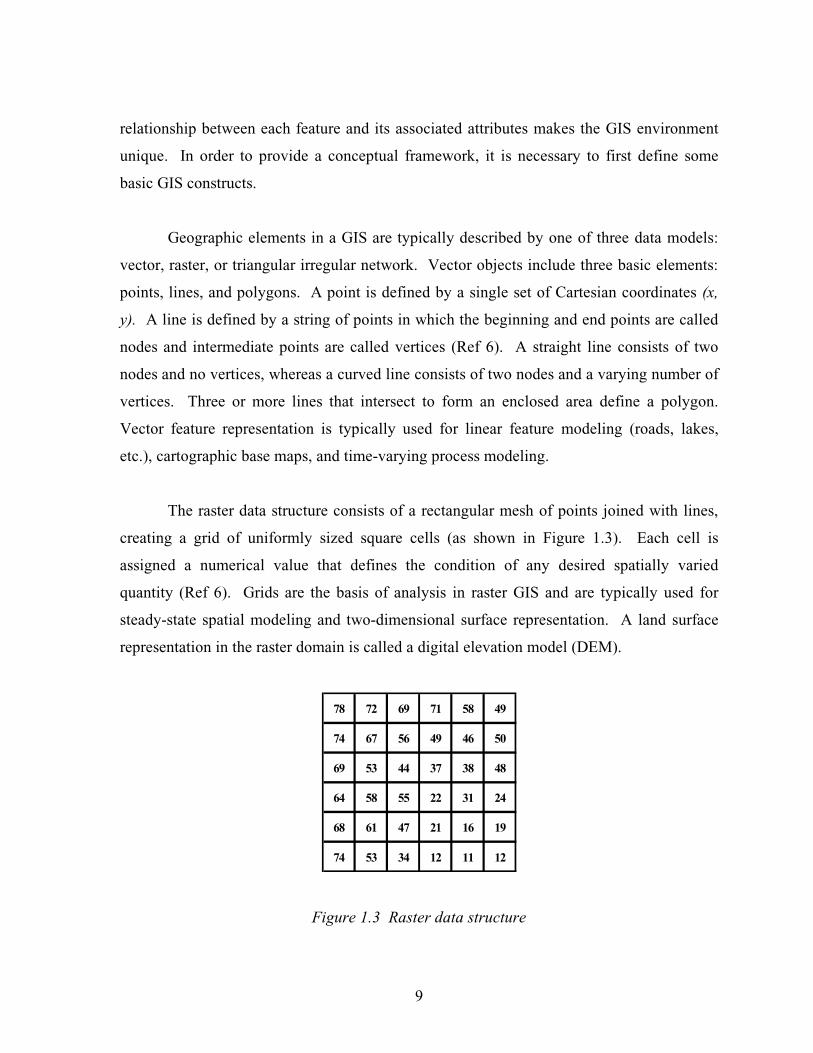
The raster data structure consists of a rectangular mesh of points joined with lines,

creating a grid of uniformly sized square cells (as shown in Figure 1.3). Each cell is

assigned a numerical value that defines the condition of any desired spatially varied

quantity (Ref 6). Grids are the basis of analysis in raster GIS and are typically used for

steady-state spatial modeling and two-dimensional surface representation. A land surface

representation in the raster domain is called a digital elevation model (DEM).

��

��

��

��

��

��

Figure 1.3 Raster data structure

10

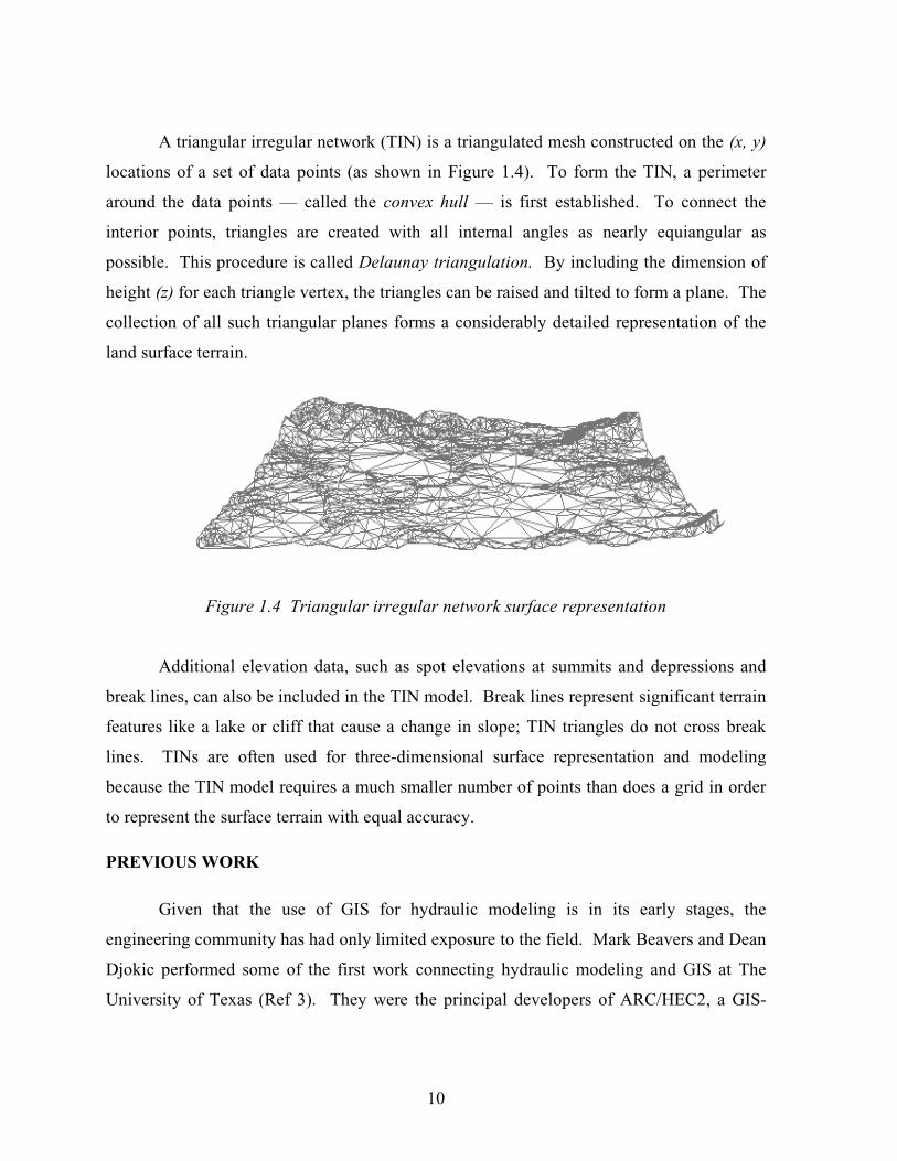
A triangular irregular network (TIN) is a triangulated mesh constructed on the (x, y)

locations of a set of data points (as shown in Figure 1.4). To form the TIN, a perimeter

around the data points — called the convex hull — is first established. To connect the

interior points, triangles are created with all internal angles as nearly equiangular as

possible. This procedure is called Delaunay triangulation. By including the dimension of

height (z) for each triangle vertex, the triangles can be raised and tilted to form a plane. The

collection of all such triangular planes forms a considerably detailed representation of the

land surface terrain.

Figure 1.4 Triangular irregular network surface representation

Additional elevation data, such as spot elevations at summits and depressions and

break lines, can also be included in the TIN model. Break lines represent significant terrain

features like a lake or cliff that cause a change in slope; TIN triangles do not cross break

lines. TINs are often used for three-dimensional surface representation and modeling

because the TIN model requires a much smaller number of points than does a grid in order

to represent the surface terrain with equal accuracy.

PREVIOUS WORK

Given that the use of GIS for hydraulic modeling is in its early stages, the

engineering community has had only limited exposure to the field. Mark Beavers and Dean

Djokic performed some of the first work connecting hydraulic modeling and GIS at The

University of Texas (Ref 3). They were the principal developers of ARC/HEC2, a GIS-

11

based tool designed to assist hydrologists in floodplain analysis. ARC/HEC2 is a set of

Arc/Info Macro Language scripts (AMLs) and C programs, which work to extract terrain

information from contour coverages, insert user-supplied information (such as roughness

coefficients, or location of left and right overbanks), and format the information into HEC-2

readable data. Following HEC-2 execution, ARC/HEC2 is capable of retrieving the HEC-2

output (in the form of water elevations at each cross section) and creating an Arc/Info

coverage of the floodplain. This process allows the resulting floodplain to be stored in a

coverage format that can be readily accessed by users who wish to use the floodplain

information in conjunction with other Arc/Info coverages. ARC/HEC2 requires that a

terrain surface be generated so that accurate cross-section profiles are provided to HEC-2.

These terrain surfaces, in the format of TINs or grids, are created within Arc/Info based on

contour lines, survey data, or other means of establishing terrain relief. The accuracy of the

surface representation is crucial for accurate floodplain calculations.

In the years following the release of ARC/HEC2, many hydrologists began to switch

from HEC-2 to the Windows-based HEC-RAS hydraulic model. RAS differed from the

HEC-2 model in that it supported import and export of GIS data. Version 2 of HEC-RAS

gives the user the option to import and utilize three-dimensional river reach and cross-

sectional data from a general-purpose data exchange file.

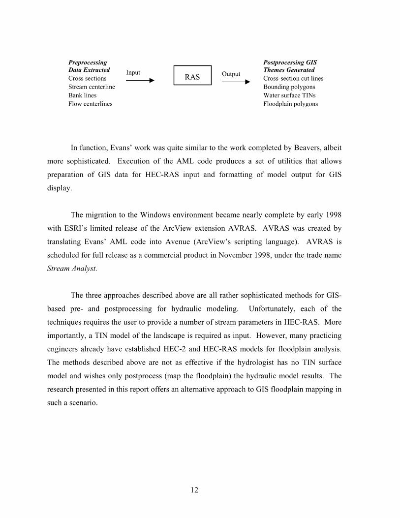
In 1997, Tom Evans of HEC released a series of AMLs that serve both as a pre- and

postprocessor for HEC-RAS. The preprocessing AMLs create a data exchange file

consisting of stream geometry description extracted from a triangular irregular network

(TIN) model of the land surface. In HEC-RAS, the user is required to provide such

additional data as Manning’s n, contraction and expansion coefficients, any hydraulic

structures (e.g., bridges, culverts), and bank stations and reach lengths (if they are not

included in the exchange file). After running the model, RAS can export the output file into

the digital-exchange file format. A TIN of the water surface can be created from the

exchange file using the postprocessing macros:

12

PreprocessingData ExtractedCross sectionsStream centerlineBank linesFlow centerlines

Postprocessing GISThemes GeneratedCross-section cut linesBounding polygonsWater surface TINsFloodplain polygons

In function, Evans’ work was quite similar to the work completed by Beavers, albeit

more sophisticated. Execution of the AML code produces a set of utilities that allows

preparation of GIS data for HEC-RAS input and formatting of model output for GIS

display.

The migration to the Windows environment became nearly complete by early 1998

with ESRI’s limited release of the ArcView extension AVRAS. AVRAS was created by

translating Evans’ AML code into Avenue (ArcView’s scripting language). AVRAS is

scheduled for full release as a commercial product in November 1998, under the trade name

Stream Analyst.

The three approaches described above are all rather sophisticated methods for GIS-

based pre- and postprocessing for hydraulic modeling. Unfortunately, each of the

techniques requires the user to provide a number of stream parameters in HEC-RAS. More

importantly, a TIN model of the landscape is required as input. However, many practicing

engineers already have established HEC-2 and HEC-RAS models for floodplain analysis.

The methods described above are not as effective if the hydrologist has no TIN surface

model and wishes only postprocess (map the floodplain) the hydraulic model results. The

research presented in this report offers an alternative approach to GIS floodplain mapping in

such a scenario.

��

13

CHAPTER 2. METHODOLOGY

The methodology detailed in this section describes approaches to processing HEC-

RAS output to enable two- and three-dimensional floodplain mapping and visualization in

ArcView GIS. The approaches are based on the assumption that the RAS cross sections are

not geographically referenced. The methodology was applied to a segment of Waller Creek

in Austin, Texas. The HEC-RAS stream cross section and flood elevation data were

imported into ArcView, in which the cross sections and floodplain were mapped along a

digital representation of the stream. A planimetric view of the floodplain was developed

using a digital orthophotograph as a base map. An approach for three-dimensional

floodplain visualization is currently under development.

The methodology for planimetric floodplain visualization consists of three primary

steps:

�� Data import from HEC-RAS,

�� Stream centerline digital representation, and

�� Cross-section georeferencing and floodplain polygon generation.

�

�These steps are discussed in detail in the following subsections.

�

�DATA IMPORT FROM HEC-RAS

�In order to move into the GIS environment, the output data from HEC-RAS must be

extracted. The first step toward this end is the creation of an output report using an HEC-

RAS menu option. The report is a text file containing input data regarding cross-sectional

geometry and flow descriptions, and output data describing water surface profiles. A

computer program written in ArcView’s scripting language, Avenue, was developed for this

project to read the RAS output text file and write key stream parameters to ArcView. The

parameters vary between cross sections and include the following:

14

�� Station number

�� Location of the minimum channel elevation

�� Bank station locations

�� Water surface elevation

�� Terrain-water surface interface locations

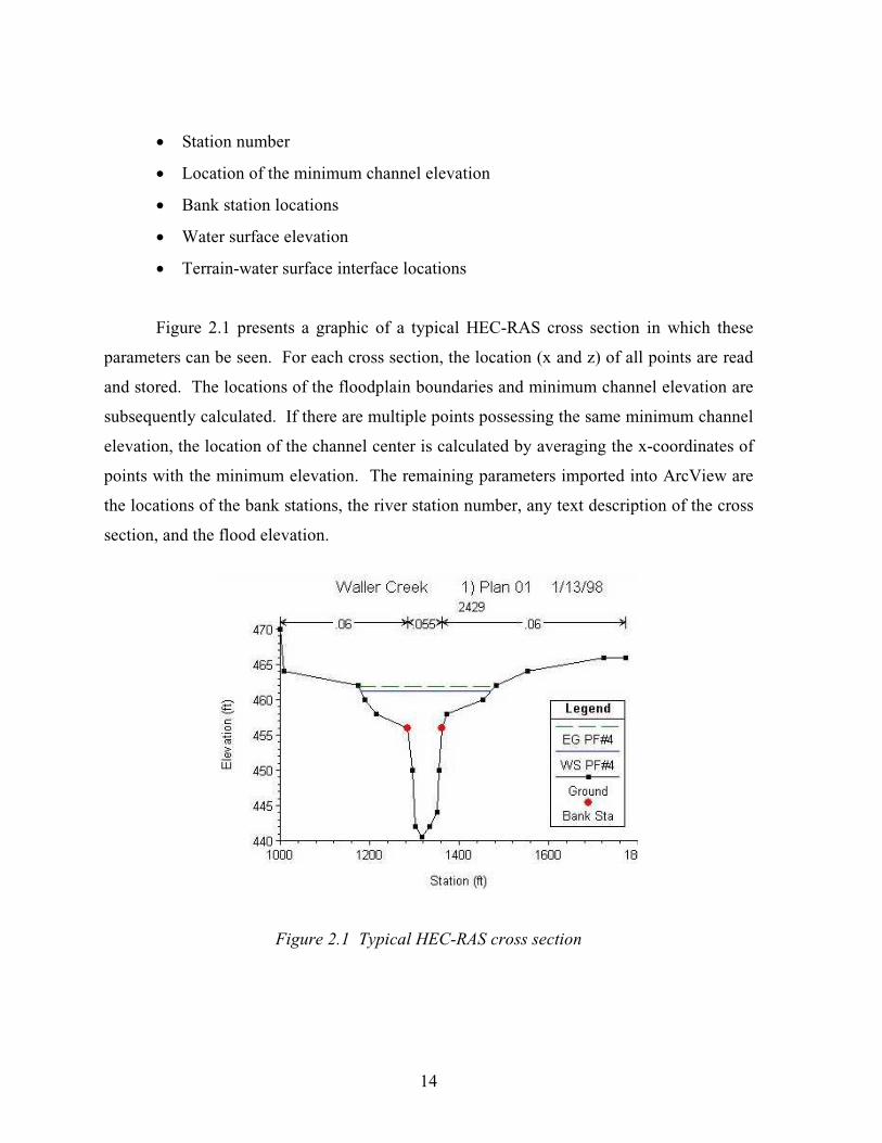
Figure 2.1 presents a graphic of a typical HEC-RAS cross section in which these

parameters can be seen. For each cross section, the location (x and z) of all points are read

and stored. The locations of the floodplain boundaries and minimum channel elevation are

subsequently calculated. If there are multiple points possessing the same minimum channel

elevation, the location of the channel center is calculated by averaging the x-coordinates of

points with the minimum elevation. The remaining parameters imported into ArcView are

the locations of the bank stations, the river station number, any text description of the cross

section, and the flood elevation.

Figure 2.1 Typical HEC-RAS cross section

15

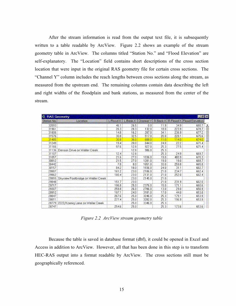
After the stream information is read from the output text file, it is subsequently

written to a table readable by ArcView. Figure 2.2 shows an example of the stream

geometry table in ArcView. The columns titled “Station No.” and “Flood Elevation” are

self-explanatory. The “Location” field contains short descriptions of the cross section

location that were input in the original RAS geometry file for certain cross sections. The

“Channel Y” column includes the reach lengths between cross sections along the stream, as

measured from the upstream end. The remaining columns contain data describing the left

and right widths of the floodplain and bank stations, as measured from the center of the

stream.

Figure 2.2 ArcView stream geometry table

Because the table is saved in database format (dbf), it could be opened in Excel and

Access in addition to ArcView. However, all that has been done in this step is to transform

HEC-RAS output into a format readable by ArcView. The cross sections still must be

geographically referenced.

16

STREAM CENTERLINE DIGITAL REPRESENTATION

The next step was to link the RAS stream to the same stream in digital form. There

are two primary ways to obtain a digital representation of a stream:

1.� Reach Files. Reach files are a series of national hydrologic databases

maintained by the U.S. Environmental Protection Agency (EPA) that uniquely

identify and interconnect the stream segments or “reaches” that comprise the

country’s surface water drainage system. The databases include such

information as unique reach codes for each stream segment,

upstream/downstream relationships, and stream names. The latest release, reach

file 3 (RF3), consists of attributed 1:100,000-scale digital line graph

hydrography. The data are available from EPA’s BASINS Website at

http://www.epa.gov/OST/BASINS/gisdata.html.

�

2.� Digitize the Stream. Using either digital orthophotographs or digital raster

graphics as a base map, the stream can be digitized using tools in ArcView.

Digital raster graphics are digitized topographic maps. Geographically

referenced digital raster graphics and orthophotos for the state of Texas can be

obtained from the Texas Natural Resources Information System (TNRIS)

Website at http://www.tnris.state.tx.us/gispage.html.

Both digital data sources were evaluated for this project. In the end, digital

orthophotos were found to provide a representation of the Waller Creek study area superior

to that provided by RF3. As such, 1-meter resolution orthophotography for the Austin East

7.5-minute quadrangle was obtained from TNRIS. In ArcView, the image was used as a

base map to digitize Waller Creek.

17

CROSS-SECTION GEOREFERENCING

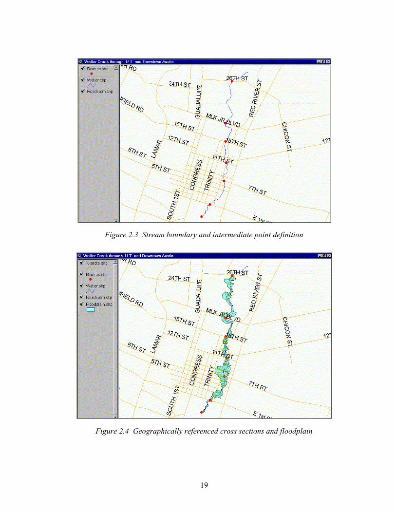
The first step toward georeferencing the cross sections is to compare the definitions

of the RAS stream and its digital counterpart. It’s entirely possible, for example, that the

digital stream is defined to a point farther upstream than the RAS stream, or vice versa.

Hence, it’s necessary to delineate the upstream and downstream boundaries of the RAS

stream on the digital stream. To this end, an Avenue script was developed, with which the

upstream and downstream boundaries can be established with a click of the mouse.

Intermediate stream definition points corresponding to important RAS cross sections, such

as bridges or culverts, can also be defined. When a point is clicked, the script determines

the nearest point along the stream centerline and snaps the point to the digital stream.

Often, the boundary points are more easily pinpointed by comparison to the location of

existing structures (e.g., roads, buildings, etc). As such, a base map theme of roads was

used in addition to the digital orthophoto to assist in the point-selection process (see Figure

2.3, page 19). As the number of defined points increases, so does the accuracy of the

resulting floodplain.

Once the stream definition points were established, the next step was to add the

cross sections between them. To do this, two attributes must be known for each cross

section: location along the stream and orientation. An Avenue script was developed to aid

in the determination of these attributes. Cross section location was determined using the

boundary points; a one-to-one relationship was established between each boundary point

and a particular cross section in the table resulting from data HEC-RAS data import (Figure

2.2). Between adjacent boundary points, the ratio of the length of the RAS modeled stream

to that of the digital stream is important. If the RAS reach lengths are correct and the

boundary points were accurately placed, then the ratio should be nearly 1. If the RAS

stream length exceeds the digital stream length, the reach lengths between cross sections

will need to be compressed by the ratio. However, if the RAS stream length is less than the

18

digital stream length, the reach lengths between cross sections should be expanded by the

same ratio. In this manner, the proportionality of RAS reach lengths is preserved.

At this point, the cross section locations are known, but not their orientation. To

determine this, an assumption was made that the cross sections occur in straight lines

perpendicular to the stream flow. This assumption was used because geographically

referenced cross-section data are typically not available. This is a key concept of this

approach. If the cross sections are “doglegged” instead of perpendicular and straight, this

approach will overestimate the floodplain width. An alternative to the assumption of

perpendicular and straight-line cross sections might be to digitize the cross sections and

attribute them with descriptive data. These data could include such information as

stationing numbering and bank station and center points identification so that the cross

sections correspond to the RAS geometry data.

The slope of the stream is determined using points located at a user-defined distance

upstream and downstream of the cross section. If the resulting cross sections intersect near

bends in the stream, the script can be re-run using a higher distance value. As the distance

value increases, so does the departure from a true perpendicular cross section. The slope of

the cross-section line is determined by calculating the negative inverse of the stream slope.

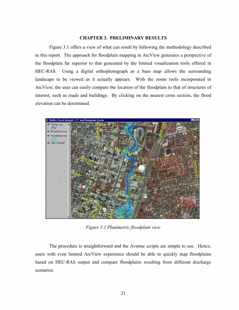
With the cross section locations and orientations now known, a line representing the

floodplain at each cross section can be formed. By connecting the ends of each cross

section, a polygon representing the floodplain extent is mapped (Figure 2.4).

19

Figure 2.3 Stream boundary and intermediate point definition

Figure 2.4 Geographically referenced cross sections and floodplain

21

CHAPTER 3. PRELIMINARY RESULTS

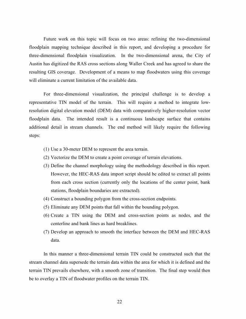
Figure 3.1 offers a view of what can result by following the methodology described

in this report. The approach for floodplain mapping in ArcView generates a perspective of

the floodplain far superior to that generated by the limited visualization tools offered in

HEC-RAS. Using a digital orthophotograph as a base map allows the surrounding

landscape to be viewed as it actually appears. With the zoom tools incorporated in

ArcView, the user can easily compare the location of the floodplain to that of structures of

interest, such as roads and buildings. By clicking on the nearest cross section, the flood

elevation can be determined.

Figure 3.1 Planimetric floodplain view

The procedure is straightforward and the Avenue scripts are simple to use. Hence,

users with even limited ArcView experience should be able to quickly map floodplains

based on HEC-RAS output and compare floodplains resulting from different discharge

scenarios.

22

Future work on this topic will focus on two areas: refining the two-dimensional

floodplain mapping technique described in this report, and developing a procedure for

three-dimensional floodplain visualization. In the two-dimensional arena, the City of

Austin has digitized the RAS cross sections along Waller Creek and has agreed to share the

resulting GIS coverage. Development of a means to map floodwaters using this coverage

will eliminate a current limitation of the available data.

For three-dimensional visualization, the principal challenge is to develop a

representative TIN model of the terrain. This will require a method to integrate low-

resolution digital elevation model (DEM) data with comparatively higher-resolution vector

floodplain data. The intended result is a continuous landscape surface that contains

additional detail in stream channels. The end method will likely require the following

steps:

(1)�Use a 30-meter DEM to represent the area terrain.

(2)�Vectorize the DEM to create a point coverage of terrain elevations.

(3)�Define the channel morphology using the methodology described in this report.

However, the HEC-RAS data import script should be edited to extract all points

from each cross section (currently only the locations of the center point, bank

stations, floodplain boundaries are extracted).

(4)�Construct a bounding polygon from the cross-section endpoints.

(5)�Eliminate any DEM points that fall within the bounding polygon.

(6)�Create a TIN using the DEM and cross-section points as nodes, and the

centerline and bank lines as hard breaklines.

(7)�Develop an approach to smooth the interface between the DEM and HEC-RAS

data.

In this manner a three-dimensional terrain TIN could be constructed such that the

stream channel data supersede the terrain data within the area for which it is defined and the

terrain TIN prevails elsewhere, with a smooth zone of transition. The final step would then

be to overlay a TIN of floodwater profiles on the terrain TIN.

23

REFERENCES

1.� Streeter, V. L., and E. B. Wylie. 1985. Fluid Mechanics, 8th ed. McGraw-Hill

Publishing Company, New York, NY.

2.� Prasuhn, A. L. 1992. Fundamentals of Hydraulic Engineering. Oxford University

Press, New York, NY.

3.� Beavers, M. A. 1994. Floodplain Determination Using HEC-2 and Geographic

Information Systems. Master’s thesis, Department of Civil Engineering, The University

of Texas at Austin.

4.� U.S. Army Corps of Engineers, Hydrologic Engineering Center. 1997. HEC-RAS River

Analysis System: Hydraulic Reference Manual. Hydrologic Engineering Center, Davis,

CA.

5.� U.S. Geological Survey. 1998. Internet: http://www.usgs.gov/research/gis/title.html.

6.� Smith, P. 1995. Hydrologic Data Development System. Department of Civil

Engineering, The University of Texas at Austin. CRWR Online Report 95-1.

gis floodplain mapping in d highway d fctr.utexas.edu/wp-content/uploads/pubs/1738_4.pdf · gis for...

Documents