giunti semirigidi con barre incollate per...
TRANSCRIPT

Università degli Studi di Trento Università degli Studi di Bergamo
Università degli Studi di Brescia Università degli Studi di Padova Università degli Studi di Trieste Università degli Studi di Udine
Università IUAV di Venezia
Mauro Andreolli
GIUNTI SEMIRIGIDI CON BARRE INCOLLATE PER STRUTTURE LIGNEE
Prof. Maurizio Piazza Dott. Roberto Tomasi
2011

II
UNIVERSITA’ DEGLI STUDI DI TRENTO Dottorato di Ricerca in “Ingegneria dei Sistemi Strutturali Civili e Meccanici” XXIII ciclo Coordinatore della Scuola di Dottorato: Prof. Davide Bigoni Esame Finale: 7 / 04 / 2011 Commissione Esaminatrice: Prof. Piazza Maurizio (Università degli Studi di Trento) Prof. Marotti De Sciarra Francesco (Università di Napoli Federico II) Prof. Joan Ramon Casas (Universitat Politecnica de Catalunya)

III
SOMMARIO
Il lavoro di tesi riguarda la caratterizzazione meccanica di un giunto, adatto per la realizzazione di differenti configurazioni in strutture intelaiate pesanti di legno, costituito da un elemento metallico flangiato collegato agli elementi strutturali in legno per mezzo di barre incollate. Questo sistema di connessione presenta alcune interessanti proprietà meccaniche in termini di prestazioni meccaniche, versatilità e prefabbricazione. Un modello analitico in grado di valutare la risposta del giunto in termini dei parametri meccanici chiave (modalità di rottura, resistenza ultima, rigidezza e capacità rotazionale) è stato proposto e validato attraverso un’ampia campagna sperimentale. A tale scopo il metodo per componenti, originariamente proposto per giunti semi-rigidi in acciaio, è stato adattato per modellare i giunti acciaio-legno, consentendo l'applicazione del capacity design e permettendo di progettare connessioni in grado di presentare valori di duttilità necessari ad applicazioni in campo sismico. Le prove effettuate hanno mostrato una soddisfacente rispondenza tra i risultati teorici e quelli sperimentali: in particolare la previsione affidabile delle modalità di rottura del giunto, permette la progettazione di connessioni resistenti a momento in grado di presentare alte deformazioni plastiche senza fenomeni di rotture fragili, con un notevole grado di duttilità strutturale a livello globale e di dissipazione energetica in seguito a sisma.

IV

V
SUMMARY
This thesis investigates the mechanical characterisation of a joint, suitable for different configurations within a heavy timber frame, consisting of a wooden element connected to a steel stub by means of an end-plate and glued-in steel rods. This connection system has some interesting properties in terms of mechanical performance, versatility and prefabrication. An analytical model to predict the joint response in terms of its key parameters (e.g. failure mode, ultimate resistance, stiffness and rotation capacity) is proposed and validated through an extensive experimental programme. The component method, originally proposed for semi-rigid joints in steel frameworks, is adapted in order to set up a feasible general model for steel–timber joints, enabling application of the capacity design approach and offering the required ductility for applications in seismic zones. The tests carried out indicate satisfactory agreement between theoretical and experimental results: the reliable prediction of joint failure modes allows design of moment-resistant connections that can sustain high plastic deformation without brittle rupture, with a remarkable degree of global ductility and energy dissipation under alternate loading.

VI

VII
Ho più ricordi che se avessi mille anni (Baudelaire)

VIII

IX
RINGRAZIAMENTI
Ringrazio il Prof. Maurizio Piazza e Roberto Tomasi per avermi seguito con pazienza e professionalità nel corso degli anni di Dottorato. Per i consigli e il lavoro realizzato assieme, presso il Laboratorio di Prove Materiali e Strutture del Dipartimento di Ingegneria Meccanica e Strutturale dell’Università di Trento, ringrazio Ivan Brandolise, Luca Corradini, Tiziano Dalla Torre, Alfredo Pojer e l’ingegner Marco Molinari. Ricordo infine con piacere e riconoscenza i tesisti e i colleghi dottorandi. Ringrazio promo_legno per la sensibilità dimostrata nel cogliere il valore della ricerca per l’evoluzione delle costruzioni in legno, avendo contribuito a sostenere finanziariamente questi anni di studio.

X

XI
INDICE
SOMMARIO ........................................................................................................... III
SUMMARY ............................................................................................................. V
RINGRAZIAMENTI ................................................................................................ IX
INDICE .................................................................................................................. XI
1. INTRODUZIONE ................................................................................................ 1 1.1 Background ................................................................................................................ 1 1.2 Organizzazione della tesi ........................................................................................... 1
2. GIUNTI SEMIRIGIDI PER STRUTTURE IN LEGNO IN ZONA SISMICA ......... 5 2.1 Fragilità a rottura degli elementi in legno ................................................................... 5
2.1.1 Tecnologie impiegate per la realizzazione di travi lignee pseudoduttili ............... 5 2.1.2 Travi in legno lamellare misto ............................................................................. 6 2.1.3 Travi in legno rinforzate con elementi metallici ................................................... 7 2.1.4 Travi rinforzate con fibre di vetro e carbonio ..................................................... 10
2.2 Duttilità nelle strutture in legno ................................................................................. 11 2.2.1 Sistemi costruttivi per costruzioni in legno ........................................................ 12 2.2.2 Sistemi costruttivi per strutture intelaiate “pesanti” in legno .............................. 14 2.2.3 Barre metalliche incollate in elementi lignei ...................................................... 15
2.3 Il giunto studiato ....................................................................................................... 17 2.4 Bibliografia ............................................................................................................... 17
3. IL METODO PER COMPONENTI .................................................................... 21 3.1 Il giunto analizzato ................................................................................................... 21 3.2 Schematizzazione del giunto semirigido .................................................................. 21 3.3 Il metodo per componenti ......................................................................................... 23 3.4 Valutazione della resistenza del giunto .................................................................... 24 3.5 Elemento a T equivalente in trazione ....................................................................... 25 3.6 Elemento a T equivalente in compressione ............................................................. 27 3.7 Resistenza dell’ala compressa del profilo metallico ................................................. 29 3.8 Resistenza delle barre incollate ............................................................................... 29
3.8.1 Resistenza assiale delle barre incollate ............................................................ 29 3.8.2 Resistenza a taglio delle barre incollate ............................................................ 29

XII
3.9 Valutazione della rigidezza del giunto ...................................................................... 30 3.10 Rigidezza flangia d’estermità in zona tesa ............................................................. 30 3.11 Rigidezza delle barre tese ...................................................................................... 31
3.11.1 Relazioni di calcolo ......................................................................................... 31 3.11.2 Valutazione del parametro α ........................................................................... 32
3.12 Rigidezza del legno in compressione ..................................................................... 38 3.12.1 Relazioni di calcolo ......................................................................................... 38 3.11.2 Valutazione del parametro β ........................................................................... 38
3.13 Valutazione della capacità rotazionale del giunto .................................................. 40 3.14 Valutazione della capacità deformativa del T-stub in trazione ............................... 42 3.15 Bibliografia ............................................................................................................. 43
4. VALIDAZIONE DEL MODELLO ANALITICO MEDIANTE ANALISI
SPERIMENTALE .................................................................................................. 45 4.1 Descrizione della campagna sperimentale ............................................................... 45
4.1.1 Geometria dei provini testati ............................................................................. 45 4.1.2 Materiali dei provini testati ................................................................................. 46 4.1.3 Realizzazione dei provini .................................................................................. 47
4.2 Set-up e protocollo di prova ..................................................................................... 48 4.2.1 Set-up di prova .................................................................................................. 48 4.2.2 Protocollo di prova ............................................................................................ 50
4.3 Prove di carico monotone ........................................................................................ 51 4.3.1 Test P6-sp ......................................................................................................... 53 4.3.2 Test P6.............................................................................................................. 54 4.3.3 Test P8-sp ......................................................................................................... 55 4.3.4 Test P8.............................................................................................................. 56 4.3.5 Test P10-sp ....................................................................................................... 57 4.3.6 Test P10............................................................................................................ 58 4.3.7 Test P15-sp ....................................................................................................... 59 4.3.8 Test P20-sp ....................................................................................................... 60 4.3.9 Confronto tra le curve carico-spostamento sperimentali ................................... 61 4.3.10 Confronto tra le curve momento-rotazione analitiche e sperimentali .............. 62
4.4 Prove di carico cicliche ............................................................................................ 67 4.4.1 Protocollo di prova adottato .............................................................................. 67 4.4.2 Test P6-sp ......................................................................................................... 72 4.4.3 Test P6.............................................................................................................. 73 4.4.4 Test P8-sp ......................................................................................................... 74 4.4.5 Test P8.............................................................................................................. 75
XIII
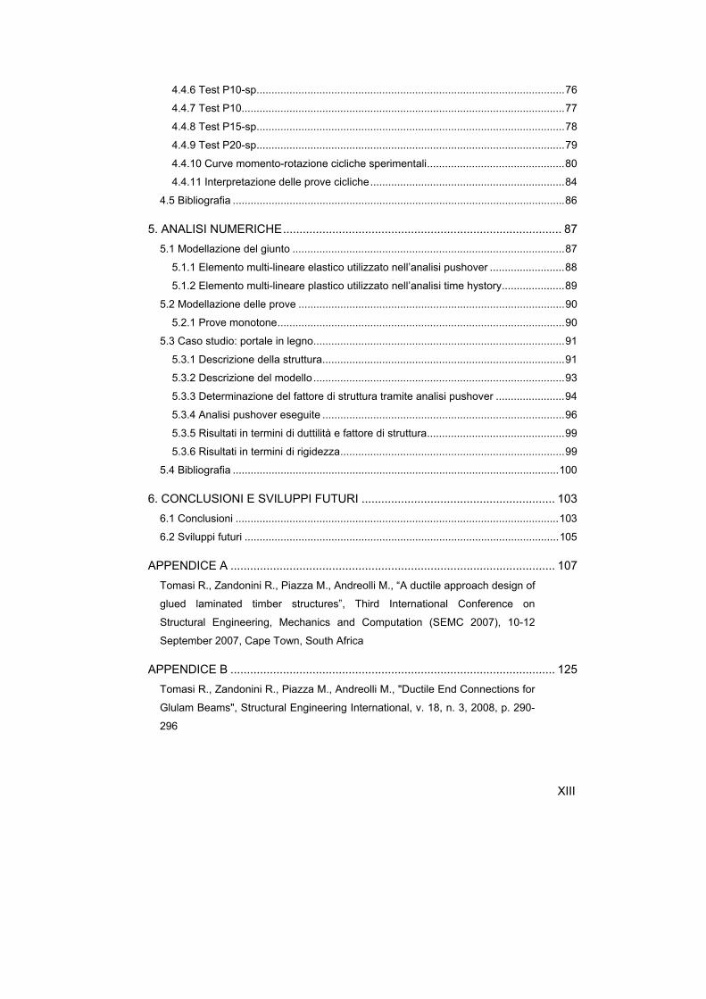
4.4.6 Test P10-sp ....................................................................................................... 76 4.4.7 Test P10............................................................................................................ 77 4.4.8 Test P15-sp ....................................................................................................... 78 4.4.9 Test P20-sp ....................................................................................................... 79 4.4.10 Curve momento-rotazione cicliche sperimentali .............................................. 80 4.4.11 Interpretazione delle prove cicliche ................................................................. 84
4.5 Bibliografia ............................................................................................................... 86
5. ANALISI NUMERICHE ..................................................................................... 87 5.1 Modellazione del giunto ........................................................................................... 87
5.1.1 Elemento multi-lineare elastico utilizzato nell’analisi pushover ......................... 88 5.1.2 Elemento multi-lineare plastico utilizzato nell’analisi time hystory ..................... 89
5.2 Modellazione delle prove ......................................................................................... 90 5.2.1 Prove monotone ................................................................................................ 90
5.3 Caso studio: portale in legno .................................................................................... 91 5.3.1 Descrizione della struttura ................................................................................. 91 5.3.2 Descrizione del modello .................................................................................... 93 5.3.3 Determinazione del fattore di struttura tramite analisi pushover ....................... 94 5.3.4 Analisi pushover eseguite ................................................................................. 96 5.3.5 Risultati in termini di duttilità e fattore di struttura .............................................. 99 5.3.6 Risultati in termini di rigidezza ........................................................................... 99
5.4 Bibliografia ............................................................................................................. 100
6. CONCLUSIONI E SVILUPPI FUTURI ........................................................... 103 6.1 Conclusioni ............................................................................................................ 103 6.2 Sviluppi futuri ......................................................................................................... 105
APPENDICE A ................................................................................................... 107 Tomasi R., Zandonini R., Piazza M., Andreolli M., “A ductile approach design of
glued laminated timber structures”, Third International Conference on
Structural Engineering, Mechanics and Computation (SEMC 2007), 10-12
September 2007, Cape Town, South Africa
APPENDICE B ................................................................................................... 125 Tomasi R., Zandonini R., Piazza M., Andreolli M., "Ductile End Connections for
Glulam Beams", Structural Engineering International, v. 18, n. 3, 2008, p. 290-
296

XIV
APPENDICE C ................................................................................................... 149 Andreolli M., Piazza M., Tomasi R., Zandonini R., “Ductile moment resistant
steel to timber connections”, SPECIAL ISSUE IN TIMBER ENGINEERING,
Proceedings of the Institution of Civil Engineers, Structures and Buildings, in
press (2011)

1
1. INTRODUZIONE
1.1 Background
In passato nel nostro paese il legno è stato utilizzato prevalentemente per le coperture di abitazioni civili o per la realizzazione di grandi strutture in legno lamellare (quali capannoni, passerelle, palestre,ecc.), strutture caratterizzate in genere da schemi isostatici o debolmente iperstatici (archi a tre cerniere, travi in semplice appoggio, portali incernierati alla base, ecc.). Negli ultimi anni si è vista una rapida diffusione di edifici multipiano realizzati con struttura interamente in legno, i quali rappresentano una valida alternativa alle più comuni soluzioni analoghe in cemento armato o muratura. Lo sviluppo e la diffusione di sistemi costruttivi in legno a setti portanti secondo diverse modalità realizzative, a parete massiccia (sistema XLAM) o intelaiata “leggera” (sistema platform frame), hanno dimostrato la validità e la competitività delle strutture in legno nell’edilizia abitativa. In seguito a diversi studi e prove sperimentali è stata dimostrata la possibilità di costruire abitazioni multipiano a setti portanti anche in zona sismica ottenendo ottimi risultati in termini di duttilità e capacità dissipativa della struttura a fronte di un evento sismico. Il tema di ricerca investigato riguarda la realizzazione di edifici intelaiati “pesanti”: tali strutture sono utilizzate soprattutto per edifici industriali, ma sono presenti anche alcuni esempi di edifici multipiano. Si tratta di costruzioni in grado di fornire ampi spazi non interrotti da setti: si prestano quindi sia all’edilizia abitativa, sia ad ospitare attività commerciali e produttive. La progettazione di edifici intelaiati in legno lamellare in zona sismica richiede lo sviluppo di giunti a momento in grado di resistere a sollecitazioni cicliche, in grado di esibire un buon comportamento duttile.
1.2 Organizzazione della tesi
La tesi verte sullo studio del comportamento in ambito sismico di nodi semirigidi per strutture lignee ottenuti mediante barre incollate. Si propone di realizzare un giunto ottenuto tramite un elemento metallico flangiato collegato alle travi in legno per mezzo di barre filettate incollate (figura 1.1): lo scopo è quello di progettare un collegamento duttile, in grado di consentire a rottura alte rotazioni plastiche, preservando l'integrità delle parti lignee. A differenza di altre soluzioni presenti in letteratura o in realizzazioni recenti, si concentra la duttilità nel nodo grazie allo snervamento di una flangia metallica progettata ad hoc.

2
La prima parte del lavoro è stata dedicata all’analisi delle risorse di duttilità nelle strutture in legno, sia in riferimento alle tecnologie impiegate per migliorare il comportamento post-elastico degli elementi lignei mediante rinforzi, sia in riferimento ai collegamenti. Nel caso di connettori a gambo cilindrico (quali chiodi, perni e bulloni) la duttilità è legata alla formazione di cerniere plastiche negli elementi di acciaio, mentre nel caso di unioni con barre incollate, in letteratura si trovano diversi studi relativi allo studio della duttilità legata allo snervamento della barra a trazione, prima che si manifestino rotture fragili dell’incollaggio. Il capitolo 3 descrive la modellazione del comportamento flessionale del giunto proposto tramite il "metodo per componenti", originariamente sviluppato per le strutture metalliche, al fine di giungere a caratterizzarne le proprietà meccaniche in termini di rigidezza, resistenza e capacità rotazionale. Si sono quindi identificati i componenti di base del collegamento, valutate le loro caratteristiche di rigidezza, resistenza e deformazione ultima, ed infine, mediante una procedura di assemblaggio, si è giunti alla valutazione delle caratteristiche meccaniche dell'intero collegamento. La scomposizione del giunto in una serie di componenti fondamentali ha permesso inoltre di applicare il principio del "capacity design": dato che la resistenza del giunto è legata a quella del componente più debole, è sufficiente garantire che tale elemento presenti un comportamento duttile per ottenere una buona duttilità a livello globale. Il capitolo 4 illustra la validazione mediante test sperimentali del modello analitico formulato: i risultati dei test eseguiti indicano buoni valori di duttilità statica e una sostanziale rispondenza del modello ai valori sperimentali. In particolare il confronto tra la relazione tri-lineare analitica e le curve momento-rotazione sperimentali evidenzia come il modello fornisca risultati molto affidabili. Sono state quindi eseguite delle prove cicliche sui giunti progettati con diversi spessori di flangia, al fine di valutarne le capacità dissipative a seguito di carichi di tipo ciclico. Il capitolo 5 presenta alcune analisi numeriche ad elementi finiti volte a valutare, con riferimento al caso studio di un portale ligneo, il fattore di struttura relativo a strutture realizzate con giunti caratterizzati da un diverso spessore delle flange, ottenendo, per le modalità di rottura dei nodi più duttili, valori paragonabili a quelli di analoghe costruzioni in acciaio.

3
Il capitolo 6 illustra le conclusioni e presenta alcune possibili prospettive future di indagine. In appendice si riportano i paper inerenti l’argomento di tesi ad oggi pubblicati. L’appendice A “A ductile approach design of glued laminated timber structures” riguarda lo studio di tecniche di rinforzo di elementi lignei mediante barre incollate in acciaio allo scopo di migliore il comportamento a rottura delle travi in legno e presenta il giunto in esame ed una prima campagna di prove sperimentali di tipo monotono. L’appendice B “Ductile end connections for glulam beams” descrive in modo esaustivo la modellazione del giunto tramite il metodo per componenti, confrontando i risultati analitici con quelli dei test sperimentali. L’appendice C “Ductile moment resistant steel to timber connections” presenta una seconda campagna di test sperimentali, sia di tipo monotono che di tipo ciclico.
Figura 1.1. Possibili applicazioni in portali in legno del giunto analizzato: nodi d’angolo resistenti a momento e giunti di base

4

5
2. GIUNTI SEMIRIGIDI PER STRUTTURE IN LEGNO IN ZONA SISMICA
2.1 Fragilità a rottura degli elementi in legno
La duttilità strutturale, ovvero la capacità di sopportare grandi deformazioni plastiche senza manifestare modalità di rottura fragili, è una caratteristica fondamentale per la progettazione di strutture in zone sismiche. Il legno è considerato, in dimensioni strutturali, un materiale fragile: gli elementi in legno, a causa della presenza di difetti (quali i nodi) e alla mancanza di omogeneità, a differenza di elementi in acciaio o calcestruzzo armato opportunamente progettati, mostrano un comportamento fragile a flessione.
Figura 2.1. Comportamento carico-spostamento (a) pseudoduttile per un provino di legno netto (b) fragile per un provino di legno in dimensioni d’uso, con l’inevitabile presenza di difetti
2.1.1 Tecnologie impiegate per la realizzazione di travi lignee pseudoduttili
Il miglioramento del comportamento post-elastico di travi in legno lamellare è stato oggetto di diverse ricerche. La duttilità di una sezione in legno lamellare può essere migliorata rinforzando la sezione al lembo teso così da favorire la plasticizzazione delle fibre compresse, aumentando quindi le risorse post-elastiche dell’elemento strutturale. Le soluzioni sviluppate a tale scopo, illustrate nella figura 2.2, considerano:
• utilizzo di lamelle aventi diversa resistenza:
− accoppiamento di lamelle di classi diverse (legno lamellare composito);

6
− accoppiamento di lamelle di specie legnose diverse (legno lamellare bispecie);
• utilizzo di sezioni allargate inferiormente
• utilizzo di rinforzi realizzati con:
− barre o lamine d’acciaio;
− fibre di vetro;
− fibre di carbonio.
Figura 2.2. Esempi tipici di sezioni aventi comportamento ultimo pseudoduttile
2.1.2 Travi in legno lamellare misto
I benefici in termini di efficienza strutturale che si possono ottenere tramite l’accoppiamento di lamelle di specie legnose diverse o di resistenza meccanica decrescente dal lembo inferiore al lembo superiore sono stati indagati in passato da diversi autori (Biblis, 1966; Moody, 1974). Più recentemente (Castro e Paganini, 1999) si è ripreso questo tema proponendo l’impiego in ambito strutturale di specie legnose caratterizzate da cicli rapidi di accrescimento quali l’eucalipto ed il pioppo. Tali specie possono, per diverse ragioni, costituire una valida alternativa all’uso di legname importato nel nostro paese:
• motivazioni di natura economica: in Italia esiste una grande diffusione di coltivazioni di pioppo, il cui legname viene impiegato principalmente nella produzione di segati, pannelli o di cellulosa per l’industria della carta;
• motivazioni di natura meccanica: diverse campagne sperimentali hanno mostrato come il pioppo presenti bassi valori di densità e resistenza a compressione parallela alle fibre rendendolo un materiale adatto all’impiego nelle zone intorno all’asse neutro, mentre l’eucalipto, grazie a valori più elevati di resistenza a trazione parallela alle fibre, possa essere utilizzato in zona tesa.

7
La compatibilità dell’accoppiamento di tali specie legnose con quelle tradizionalmente impiegate in ambito strutturale, principalmente l’abete ed il larice, è stata verificate inoltre in diversi studi (Lantos, 1970), fugando eventuali dubbi relativi alla possibilità di delaminazioni in conseguenza di un differente comportamento igrometrico dei diversi materiali.
Figura 2.3. Travi in legno lamellare misto: (a) legno lamellare bispecie (b) legno lamellare combinato
2.1.3 Travi in legno rinforzate con elementi metallici
L’impiego di travi in legno con elementi di rinforzo nasce da esigenze diverse da quella di migliorare il comportamento a rottura degli elementi lignei, esigenze legate invece alla possibilità di ottenere sezioni con maggiori resistenza e rigidezza. I settori in cui si sono applicate tali tecniche riguardano sia il recupero di elementi tradizionali in legno massiccio, che la produzione di nuovi elementi in legno lamellare rinforzato. Le tecniche utilizzate possono essere divise in base a:
• tipo di rinforzo: barre, piatti, strisce, cavi;
• tipo di materiale: acciaio,alluminio, materiali compositi quali fibra di vetro e fibra di carbonio.
In letteratura si trovano molteplici tipologie di rinforzo strutturale: in particolare quelli che hanno ottenuto maggiore successo sono stati i rinforzi realizzati con barre d’acciaio, le cui prime applicazioni, sia per quanto riguarda il legno massiccio che il legno lamellare, risalgono agli anni ’60. Nelle travi armate realizzate da Lantos (Lantos, 1970), le barre venivano preliminarmente bagnate con un primer a base di lattice, alloggiate successivamente in apposite sedi effettuate nelle lamelle e rese solidali al legno mediante la stessa colla utilizzata per l’incollaggio delle lamelle (adesivi a base di fenol-resorcinol-formaldeide).

8
Lantos dimostra che l’ipotesi di perfetta aderenza tra acciaio e legno è pienamente giustificata, in quanto la deformabilità dello strato di adesivo non condiziona sostanzialmente i risultati che si ottengono con il modello di trave omogeneizzata, descrivendo il comportamento della sezione in legno armato analogamente a quello di una sezione in calcestruzzo armato. Tale ricerca ha portato inoltre alle seguenti conclusioni:
• la variabilità delle prestazioni delle travi armate risulta sostanzialmente inferiore a quella delle travi convenzionali e quindi si può prevedere un aumento delle tensioni ammissibili utilizzate nella determinazione della resistenza delle sezioni omogeneizzate;
• le travi in legno armato sono caratterizzate da un’ottima risposta ai carichi ciclici: alcune travi, sottoposte a 100.000 cicli tra 0,5 e 1,5 volte il carico di progetto, non hanno mostrato alcun deterioramento della risposta strutturale. In particolare dopo i primi 1000 cicli i valori delle deformazioni flessionali sono rimasti pressoché invariati;
• le barre di armatura con diametro maggiore di 12 mm hanno manifestato la tendenza ad essere soggette a fenomeni prematuri di perdita di aderenza, sostanzialmente a causa delle difficoltà realizzative e di incollaggio;
• la sezione omogeneizzata presenta un notevole incremento di rigidezza e resistenza: con una percentuale di armatura pari ad 1,5% si può ottenere un aumento dal 50 al 60 % delle capacità prestazionali rispetto alla trave di partenza;
• nella fabbricazione di travi armate possono essere utilizzate specie legnose meno resistenti, in genere non impiegate per scopi strutturali;
• è necessario adottare metodi di incollaggio che garantiscano una
resistenza della linea di colla maggiore di quella a taglio del legno.
Figura 2.4. Esempi di sezioni in legno armato (Lantos, 1970)
9
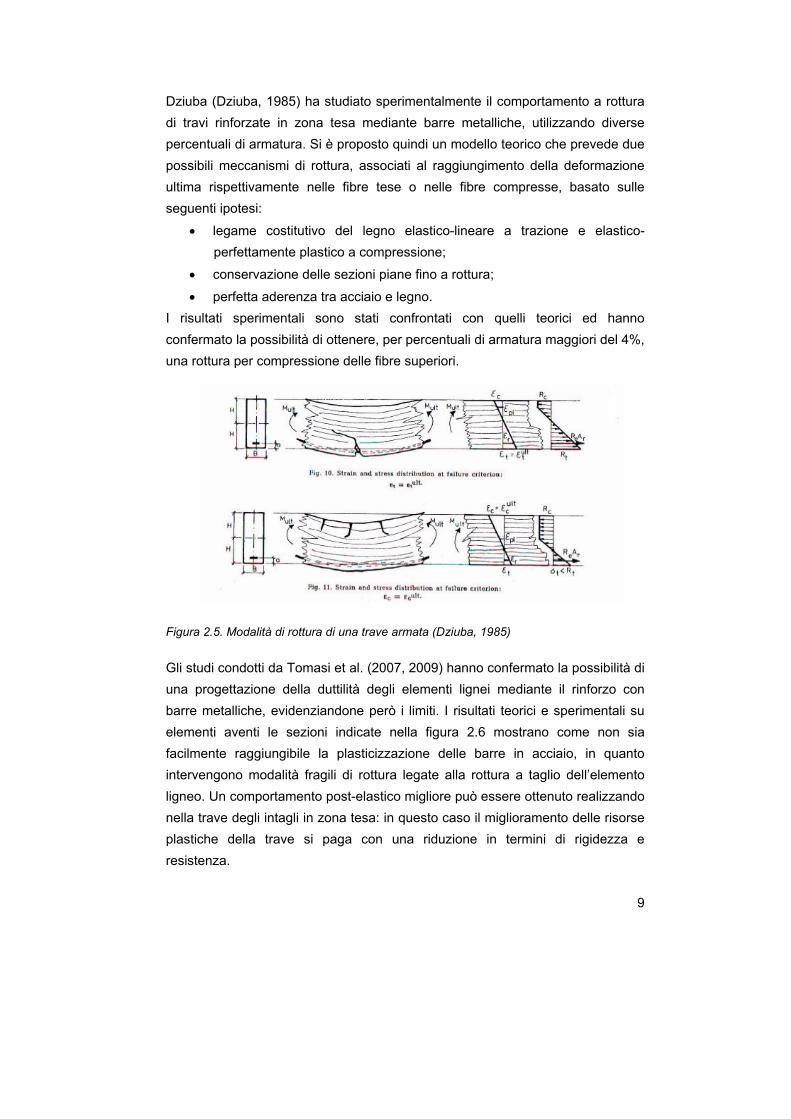
Dziuba (Dziuba, 1985) ha studiato sperimentalmente il comportamento a rottura di travi rinforzate in zona tesa mediante barre metalliche, utilizzando diverse percentuali di armatura. Si è proposto quindi un modello teorico che prevede due possibili meccanismi di rottura, associati al raggiungimento della deformazione ultima rispettivamente nelle fibre tese o nelle fibre compresse, basato sulle seguenti ipotesi:
• legame costitutivo del legno elastico-lineare a trazione e elastico-perfettamente plastico a compressione;
• conservazione delle sezioni piane fino a rottura;
• perfetta aderenza tra acciaio e legno. I risultati sperimentali sono stati confrontati con quelli teorici ed hanno confermato la possibilità di ottenere, per percentuali di armatura maggiori del 4%, una rottura per compressione delle fibre superiori.
Figura 2.5. Modalità di rottura di una trave armata (Dziuba, 1985)
Gli studi condotti da Tomasi et al. (2007, 2009) hanno confermato la possibilità di una progettazione della duttilità degli elementi lignei mediante il rinforzo con barre metalliche, evidenziandone però i limiti. I risultati teorici e sperimentali su elementi aventi le sezioni indicate nella figura 2.6 mostrano come non sia facilmente raggiungibile la plasticizzazione delle barre in acciaio, in quanto intervengono modalità fragili di rottura legate alla rottura a taglio dell’elemento ligneo. Un comportamento post-elastico migliore può essere ottenuto realizzando nella trave degli intagli in zona tesa: in questo caso il miglioramento delle risorse plastiche della trave si paga con una riduzione in termini di rigidezza e resistenza.

10
Figura 2.6. Sezioni di travi in legno lamallare rinforzate con barre metalliche sottoposte a test sperimentali (Tomasi et al., 2007)
Il problema principale legato al legno lamellare armato è la difficoltà di realizzarlo all’interno del ciclo tradizionale di produzione del legno lamellare. Bullet e Sandberg (1989) propongono di realizzare delle lamelle armate fatte di particelle di legno pressato ed armature ad aderenza migliorata. Tali lamelle hanno quindi un processo produttivo autonomo e vengono inserite successivamente nel pacchetto della trave in legno lamellare. La scarsa diffusione di questa tecnologia si spiega con il fatto che rallenta comunque il ciclo di produzione del lamellare e permette di ottenere elementi aventi una lunghezza massima modesta.
2.1.4 Travi rinforzate con fibre di vetro e carbonio
Negli ultimi anni sono state sperimentate, in seguito alla maggiore disponibilità e convenienza economica di tali materiali rispetto al passato, tecniche di rinforzo con fibre di vetro (GFRP) e di carbonio (CFRP). In (Borri et al., 1999) sono analizzate sperimentalmente alcune tecniche di consolidamento di strutture lignee basate sull’impiego di nastri in fibra di carbonio applicati mediante resine epossidiche. Tale metodologia di intervento rappresenta una soluzione interessante soprattutto nella conservazione del patrimonio edilizio storico: in particolare tale sistema di consolidamento basato sull’applicazione di fogli di CFRP consente la messa in opera dei nastri senza dover smontare la parte sovrastante di struttura, realizzando il rinforzo in tempi brevi e con costi relativamente contenuti. La ricerca ha riguardato principalmente i seguenti aspetti:
• la valutazione dell’aderenza tra il legno e la fibra di carbonio attraverso prove di adesione;

11
• la valutazione del comportamento flessionale a rottura;
• la valutazione della rigidezza.
I risultati ottenuti mostrano un buon comportamento sia in termini di adesione che in termini di resistenza a flessione, mentre l’incremento di rigidezza è risultato notevolmente inferiore rispetto a quello della capacità portante. In (Plevris e Triantafillou, 2000) si è dimostrato come l’utilizzo di elementi lignei rinforzati al lembo inferiore con fogli in FRP consenta un miglioramento di resistenza, rigidezza e duttilità. In particolare gli aspetti analizzati da un punto di vista teorico riguardano:
• i meccanismi di rottura;
• la capacità di carico;
• la duttilità in curvatura della sezione. In (Romani e Blaϐ, 2001) si è sviluppato un modello numerico in grado di descrivere il comportamento flessionale di un elemento ligneo rinforzato con FRP. Dato che tali materiali presentano elevati moduli elastici ed elevate deformazioni a rottura, si ottiene un notevole abbassamento dell’asse neutro della sezione e si favorisce quindi la plasticizzazione delle fibre superiori con un conseguente aumento di duttilità. In (Gentile e Svecova, 2002) si è indagato il comportamento a rottura a flessione di sezioni in legno lamellare rinforzate con fibre di vetro. Le conclusioni di tale studio sono:
• la presenza di barre in fibra di vetro al lembo inferiore permette di limitare la fessurazione dell’elemento;
• la modalità di rottura, fragile per gli elementi in legno lamellare non armato, diventa duttile per le sezioni rinforzate;
• non sono stati osservati problemi legati alla delaminazione in corrispondenza delle fibre di vetro.
2.2 Duttilità nelle strutture in legno
Le ricerche condotte al fine di ottenere una modalità di rottura in cui si abbia la plasticizzazione delle fibre compresse prima che intervenga la rottura fragile al lembo teso, aumentando le risorse post-elastiche dell’elemento strutturale, evidenziano come in realtà sia possibile solamente ottenere un fenomeno che può essere indicato con il termine “pseudoduttilità”. Si tratta di una duttilità che si manifesta solo nel caso di carichi crescenti in modo monotono e che viene a mancare in seguito all’inversione della sollecitazione: se il carico viene invertito si

12
può infatti giungere alla rottura istantanea dell’elemento, in quanto i corrugamenti del materiale ligneo conseguenti al collasso locale a compressione presentano una bassissima resistenza a trazione. Si tratta quindi di soluzioni tecnologiche non adatte a dissipare energia in seguito a sisma: di conseguenza, nelle strutture in legno, la dissipazione energetica si concentra nelle connessioni, le quali , se opportunamente dimensionate, possono resistere all’azione sismica in campo plastico. Tale principio è richiamato in modo esplicito nell’eurocodice 8: “Le zone dissipative devono essere localizzate in corrispondenza dei nodi e delle connessioni, mentre si deve assumere per le membrature di legno un comportamento elastico”. In accordo con il principio del capacity design (Paulay e Priestley, 1992), la duttilità dei nodi deve quindi essere adeguatamente progettata per garantire la richiesta duttilità globale della struttura. A questo scopo i nodi devono possedere adeguata capacità dissipativa in seguito a deformazioni cicliche, mentre gli elementi in legno devono presentare una sufficiente sovraresistenza, così da evitare meccanismi di rottura fragili fuori dalla zona di connessione. Nei connettori metallici a gambo cilindrico (ad esempio chiodi, viti, perni e bulloni), per i quali la resistenza è valutata attraverso espressioni basate sulla teoria di Johansen (1949), la duttilità è ottenuta mediante la deformazione plastica dei connettori metallici.
2.2.1 Sistemi costruttivi per costruzioni in legno
La moderna edilizia in legno presenta diverse tipologie costruttive. Nel campo dell’edilizia abitativa negli ultimi anni si è avuta una rapida diffusione di edifici multipiano realizzati a setti portanti con pareti a telaio leggero o pareti massicce di tavole incrociate tipo XLAM. Per quanto riguarda gli edifici intelaiati leggeri, si tratta di strutture molto diffuse soprattutto nel mondo anglosassone, in cui si ha un sistema costruttivo a lastre, con elementi destinati a sopportare i carichi verticali e a svolgere al contempo la funzione di irrigidimento. L’ossatura portante, con montanti disposti a distanza piuttosto ravvicinata, il telaio di legno appunto, viene rivestita con pannelli per costituire una lastra, impiegando in genere sezioni e materiali di rivestimento standard, connessi mediante semplici mezzi di collegamento quali chiodi, cambrette e viti. Quando ben progettato il sistema “platform frame” consente una grande ridondanza di percorsi di trasmissione del carico, grazie all’enorme

13
numero di elementi strutturali e di elementi di collegamento. Il risultato è la possibilità di ottenere un buon comportamento dissipativo, in seguito alla presenza di connettori metallici a gambo cilindrico di diametro ridotto (in grado di snervarsi senza innescare modalità fragili di rottura negli elementi lignei) e all’iperstaticità della struttura, che garantisce in caso di crisi di un elemento una diversa distribuzione delle azioni. Per queste ragioni le norme sismiche prevedono per queste tipologie di strutture a “pannelli di parete chiodati con diaframmi chiodati” il valore del fattore di struttura più alto per le strutture di legno (q=5).
Figura 2.7. Edificio in costruzione, pareti a telaio leggero
Le costruzioni di tipo massiccio con pannelli di tavole incrociate sono sistemi di recente introduzione. Sono caratterizzate da elementi massicci piani multistrato con funzione portante, realizzati tramite sovrapposizione di strati incrociati di tavole, uniti tra loro mediante incollaggio. Tali elementi assumono, in base alle condizioni di carico, funzione portante di piastre (nel caso dei solai) e lastre (nel caso delle pareti). La composizione alternata della sezione trasversale del compensato di tavole permette non solo una maggiore stabilità dimensionale rispetto ad altre soluzioni di legno massiccio, ma consente anche di ottenere con un unico pannello una capacità portante nelle due direzioni principali. Anche a causa della recente diffusione, fino ad ora nelle normative europee (Eurocodice 5 e 8) non viene data per questo sistema costruttivo alcuna indicazione né costruttiva né di calcolo. In questa tipologia costruttiva la duttilità è concentrata nei collegamenti tra i pannelli in legno, mentre i pannelli stessi, costituiti da tavole incollate, non consentono dissipazione energetica.

14
Figura 2.8. Edificio in costruzione, pareti massicce XLAM
La dissipazione energetica è limitata nelle soluzioni costruttive costituite da schemi pendolari controventati mediante croci di sant’Andrea o nei portali, dove la duttilità è concentrata in un basso numero di connessioni.
2.2.2 Sistemi costruttivi per strutture intelaiate “pesanti” in legno
Nella realizzazione di telai “pesanti” in legno vengono adottate in genere connessioni trave-colonna resistenti a momento ottenute mediante piastre metalliche (inserite in fresature all’interno degli elementi lignei o esterne) e connettori metallici.
Figura 2.9. Giunti trave - colonna realizzati mediante piastre metalliche e connettori
Esistono però anche altre soluzioni costruttive quali giunti a pettine a tutta sezione (realizzati secondo lo stesso principio utilizzato per la giunzione longitudinale delle lamelle per elementi in legno lamellare), oppure giunti a
15
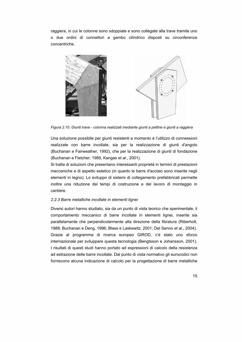
raggiera, in cui le colonne sono sdoppiate e sono collegate alla trave tramite uno o due ordini di connettori a gambo cilindrico disposti su circonferenze concentriche.
Figura 2.10. Giunti trave - colonna realizzati mediante giunti a pettine e giunti a raggiera
Una soluzione possibile per giunti resistenti a momento è l’utilizzo di connessioni realizzate con barre incollate, sia per la realizzazione di giunti d'angolo (Buchanan e Fairweather, 1992), che per la realizzazione di giunti di fondazione (Buchanan e Fletcher; 1989, Kangas et al., 2001). Si tratta di soluzioni che presentano interessanti proprietà in termini di prestazioni meccaniche e di aspetto estetico (in quanto le barre d'acciaio sono inserite negli elementi in legno). Lo sviluppo di sistemi di collegamento prefabbricati permette inoltre una riduzione dei tempi di costruzione e del lavoro di montaggio in cantiere.
2.2.3 Barre metalliche incollate in elementi lignei
Diversi autori hanno studiato, sia da un punto di vista teorico che sperimentale, il comportamento meccanico di barre incollate in elementi lignei, inserite sia parallelamente che perpendicolarmente alla direzione della fibratura (Riberholt, 1988; Buchanan e Deng, 1996; Blass e Laskewitz, 2001; Del Senno et al., 2004). Grazie al programma di ricerca europeo GIROD, c’è stato uno sforzo internazionale per sviluppare questa tecnologia (Bengtsson e Johansson, 2001). I risultati di questi studi hanno portato ad espressioni di calcolo della resistenza ad estrazione delle barre incollate. Dal punto di vista normativo gli eurocodici non forniscono alcuna indicazione di calcolo per la progettazione di barre metalliche
16
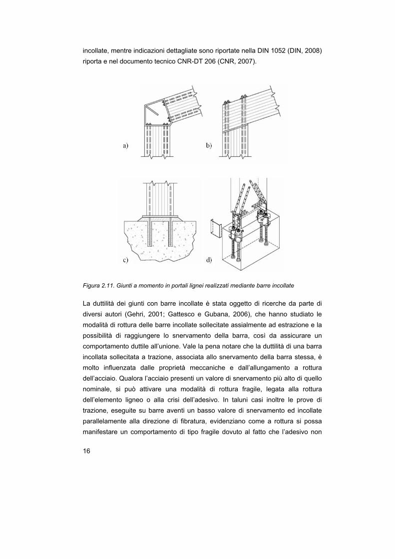
incollate, mentre indicazioni dettagliate sono riportate nella DIN 1052 (DIN, 2008) riporta e nel documento tecnico CNR-DT 206 (CNR, 2007).
Figura 2.11. Giunti a momento in portali lignei realizzati mediante barre incollate
La duttilità dei giunti con barre incollate è stata oggetto di ricerche da parte di diversi autori (Gehri, 2001; Gattesco e Gubana, 2006), che hanno studiato le modalità di rottura delle barre incollate sollecitate assialmente ad estrazione e la possibilità di raggiungere lo snervamento della barra, così da assicurare un comportamento duttile all’unione. Vale la pena notare che la duttilità di una barra incollata sollecitata a trazione, associata allo snervamento della barra stessa, è molto influenzata dalle proprietà meccaniche e dall’allungamento a rottura dell’acciaio. Qualora l’acciaio presenti un valore di snervamento più alto di quello nominale, si può attivare una modalità di rottura fragile, legata alla rottura dell’elemento ligneo o alla crisi dell’adesivo. In taluni casi inoltre le prove di trazione, eseguite su barre aventi un basso valore di snervamento ed incollate parallelamente alla direzione di fibratura, evidenziano come a rottura si possa manifestare un comportamento di tipo fragile dovuto al fatto che l’adesivo non

17
riesce a seguire le grandi deformazioni di strizione dell’acciaio a snervamento. Il risultato è una perdita di aderenza tra colla e acciaio, con una conseguente riduzione della lunghezza di ancoraggio e la rottura a taglio a livello delle fibre del legno (Gehri, 2001).
2.3 Il giunto studiato
Il giunto presentato nel seguente lavoro di tesi è ottenuto tramite un elemento metallico flangiato collegato alle travi in legno per mezzo di barre filettate incollate: lo scopo è quello di progettare un collegamento duttile, in grado di consentire a rottura alte rotazioni plastiche, preservando l'integrità delle parti lignee. A differenza di altre soluzioni presenti in letteratura o in realizzazioni recenti si concentra la duttilità nel nodo grazie allo snervamento di una flangia metallica progettata ad hoc: questo consente di ottenere giunti caratterizzati da una duttilità molto maggiore rispetto a collegamenti che sfruttano la duttilità delle barre metalliche a trazione.
2.4 Bibliografia
Bengtsson C., Johansson C.J., GIROD - Glued-in rods for timber structures, Proceedings of the 34th CIB W18 meeting, Venice, Italy, 2001, CIB W18/34-7-8.
Biblis E. J., Design considerations for laminated wood beams composed of two species, Forest Product Journal, vol. 16, n◦ 7, 1966
Blass H.J., Laskewitz B., Load-carrying capacity of axially loaded rods glued-in perpendicular to the grain, Proceedings PRO 22, International RILEM Symposium on Joints in Timber Structures, RILEM Publications S.A.R.L., Stuttgart, Germany, 2001, 363-371.
Borri A., Terenzi G., Bartoloni M., Caliterna P., Travi lignee. Tecniche di rinforzo basate su disposizioni diversificate da nastri in CFRP, L’Edilizia 13 (7/8), 1999
Buchanan A. H., Fairweather R. H., Epoxied moment-resisting connections for timber buildings, Proceedings of the International Workshop on Wood Connectors, Las Vegas, Nevada, U.S.A., 1992, 107-113.
Buchanan A.H., Deng X. J., Strength Epoxied Steel Rods in Glulam Timber, Proceedings of the International Wood Engineering Conference '96, New Orleans, U.S.A., 1996, 4, 488-495.

18
Buchanan A.H., Fletcher M.R., Glulam Portal Frame Swimming Pool Construction, Proceedings of the Second Pacific Timber Engineering Conference, Auckland, New Zealand, 1989, 1, 245-249.
Bulleit W. M., Sandberg L., Woods G., Steel-Reinforced Glued Laminated Timber, Journal of Structural Engineering, vol. 115, n◦ 2, 1989
Castro G., Paganini F., Mixed glued laminated timber of Poplar and Eucalyptus grandis clones, Holz als Roh und Werkstoff, 2003
Castro G., Paganini F., Poplar-Eucalyptus Glued Laminated Timber, EUROWOOD Technical Workshop Proceedings, 1999
CEN, European Committee for Standardization, Eurocode 5: Design of timber structures. Part 1-1: General - Common rules and rules for buildings, 2004, EN 1995-1-1.
CEN, European Committee for Standardization, Eurocode 8: Design of structures for earthquake resistance - Part 1: General rules, seismic actions and rules for buildings, 2004, EN 1998-1.
CEN, European Committee for Standardization, Eurocode 8: Design of structures for earthquake resistance - Part 1: General rules, seismic actions and rules for buildings, 2004, EN 1998-1.
CNR, National Research Council, Instruction for design, execution and control of timber structures (in Italian), 2007, CNR-DT 206/2007.
Del Senno M., Piazza M., Tomasi R., Axial glued-in steel timber joints - experimental and numerical analysis, Holz als Roh- und Werkstoff, 2004, 62, 137-146.
DIN Deutsches Institut für Normung, Design of timber structures. General rules and rules for buildings (in German), 2008, DIN 1052.
Dziuba T., The ultimative strength of wooden beams with tension reinforcement, Holzforschung und Holzverwertung, 37 (6), 1985
Gattesco N., Gubana A., Performance of Glued-in Joints of Timber Members, Proceedings of WCTE 2006 - 9th World Conference on Timber Engineering, Portland, U.S.A., 2006.

19
Gehri E., Ductile behaviour and group effect of glued-in steel rods, Proceedings PRO 22, International RILEM Symposium on Joints in Timber Structures, RILEM Publications S.A.R.L., Stuttgart, Germany, 2001, 333-342.
Gentile C., Svecova D., Timber Beams Strengthened with GFRP Bars: Development and Apllications, Journal of Composite for Construction, vol. 6, n◦ 1, 2002
Jaspart J.P., General report: session on connections, Journal of Constructional Steel Research, 2000, 55, 69-89.
Johansen K.W., Theory of Timber Connections, IABSE - International Association of Bridge and Structural Engineering, Bern, Publication No. 9, 1949, 249–262.
Kangas J., Kevarinmäki A., Lumiaho H., Timber Structures with Connections Based on in V-Form Glued-In Rods, Proceedings of IABSE Conference ‘Innovative Wooden Structures and Bridges’, Lahti, Finland, 2001, 85, 585 – 590.
Lantos G., The flexural behaviour of steel reinforced laminated timber beams, Wood Science, 1970
Moody R. C., Design criteria for larger structural glue-laminated timber beams using mixed species of visual graded lumber, USDA Forest Service, 1974
Paulay T., Priestley M.J.N., Seismic design of reinforced concrete and masonry buildings, John Wiley and Sons, 1992.
Piazza M., Tomasi R. and Modena R., Strutture in legno, Ulrico Hoepli Editore, Milano, Italia, 2005
Plevris N., Triantafillou T., FRP-Reinforced Wood and Structural Material, Journal of Material in Civil Engineering, vol. 4, 2000
Polastri A., Caratterizzazione del comportamento di giunti semirigidi per strutture lignee in zona sismica, Tesi di Dottorato, Università degli Studi di Trento, 2010
Riberholt H., Glued Bolts in Glulam - Proposal for CIB Code, Proceedings of the 21th CIB W18 meeting, Parksville, Canada, 1988, CIB W18/21-7-2.
Romani M., Blaß H. J., Design model for FRP reinforced glulam beams, Proceedings CIB-W18 Meeting, Venice, Italy, 2001

20
Tomasi R., Elementi lignei a duttilità concentrate, a duttilità diffusa e pseudoduttili: stato dell’arte, ricerca e sviluppo di tecnologie innovative, Tesi di Dottorato, Università degli Studi di Trento, 2004
Tomasi R., Piazza M., Parisi M.A., Ductile design of glued-laminated timber beams, Practice Periodical of Structural Design and Costruction ASCE, 14, No. 3, 2009, 113-122.

21
3. IL METODO PER COMPONENTI
3.1 Il giunto analizzato
Si analizza il comportamento meccanico di un giunto per elementi lignei ottenuto tramite un elemento metallico flangiato collegato alle travi in legno per mezzo di barre filettate incollate. Il giunto è formato, così come illustrato nella figura 3.1, da un profilo metallico (1) alla cui estremità è saldata una flangia metallica, collegato ad un elemento in legno lamellare (2) mediante delle barre incollate (4) e una lama incollata in una fresatura nella testa dell’elemento ligneo.
Figura 3.1. Il giunto flangiato: senza (a) o con (b) lama a scomparsa nell’elemento ligneo
Tale configurazione del giunto consente la trasmissione del momento flettente tramite le barre incollate e dell’azione tagliante tramite la lama inserita a scomparsa nell’elemento ligneo. Nel caso di presenza di forze di taglio modeste invece la trasmissione del taglio può essere affidata direttamente alle barre incollate.
3.2 Schematizzazione del giunto semirigido
Ai fini dell’analisi strutturale un collegamento può essere rappresentato da una molla rotazionale, il cui comportamento è descritto dalla relazione che lega il momento applicato Mj,Ed alla corrispondente rotazione φEd tra gli elementi strutturali collegati.

22
Figura 3.2. Modellazione del giunto mediante molle rotazionali
In accordo con l’eurocodice EN 1993-1-8 (CEN, 2005) le proprietà meccaniche che caratterizzano tale legge momento-rotazione sono le seguenti:
− momento resistente Mj,Rd
− rigidezza rotazionale Sj
− capacità di rotazione φCd
La relazione tra il momento flettente Mj,Ed applicato al giunto e la corrispondente rotazione φEd è illustrata nella figura 3.3. Tale curva consiste di tre parti:
− per valori di Mj,Ed inferiori a 2/3 di Mj,Rd si assume un andamento elastico-lineare caratterizzato dalla rigidezza rotazionale iniziale Sj,ini;
− per valori di Mj,Ed pari a Mj,Rd, con valori di rotazione superiori a φXd, si assume un andamento perfettamente plastico, trascurando quindi l’incrudimento del materiale;
− per valori di Mj,Ed compresi tra 2/3 di Mj,Rd e Mj,Rd, con valori di rotazione inferiori a φXd, si assume una rigidezza ridotta (nel caso di collegamenti con flange di estremità il parametro η vale 3).
Figura 3.3. Relazione momento-rotazione di progetto tri-lineare

23
3.3 Il metodo per componenti
Nella caratterizzazione delle proprietà meccaniche di un collegamento si può operare in diversi modi:
− sperimentazione;
− analisi numerica;
− trattazione analitica.
Si intende adottare il metodo per componenti, per procedere successivamente alla validazione del modello con prove sperimentali. Il metodo per componenti (Jaspart, 2000, EN 1993-1-8, 2005), sviluppato per le strutture metalliche, consente di valutare analiticamente la rigidezza e la resistenza di un collegamento a partire dalle caratteristiche di rigidezza e resistenza dei componenti di base in cui viene scomposto. Grazie alle indicazioni relative alla capacità deformativa ultima dei componenti base illustrata in Beg et al. (Beg et al., 2004) è possibile inoltre valutare la capacità rotazionale del giunto. L’applicazione del metodo per componenti prevede i seguenti step:
1. identificazione dei componenti di base del collegamento; 2. valutazione delle caratteristiche (rigidezza, resistenza e capacità de-
formativa) di ognuno dei componenti di base; 3. assemblaggio dei componenti per la valutazione delle caratteristiche
dell’intero collegamento.
Nella figura 3.4 sono identificati i componenti di base del giunto in esame (step 1):
Figura 3.4. Componenti di base del giunto studiato
24
Nella valutazione delle caratteristiche meccaniche di ciascun componente di base (step 2) si deve quindi considerare la presenza di componenti quali “legno in compressione” o “barre incollate” non presenti nell’eurocodice 3 per le strutture metalliche. Assemblando infine i singoli componenti (step 3) si giunge alla determinazione dell’intera curva momento-rotazione del giunto.
3.4 Valutazione della resistenza del giunto
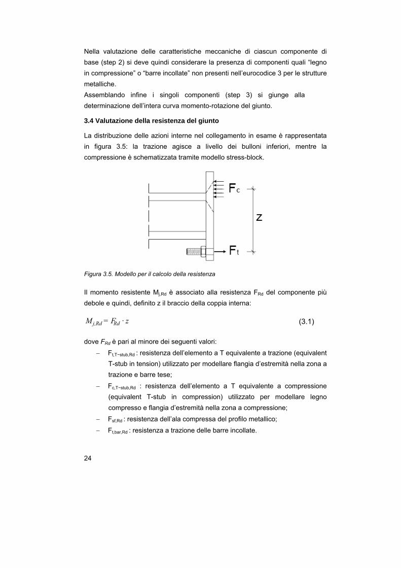
La distribuzione delle azioni interne nel collegamento in esame è rappresentata in figura 3.5: la trazione agisce a livello dei bulloni inferiori, mentre la compressione è schematizzata tramite modello stress-block.
Figura 3.5. Modello per il calcolo della resistenza
Il momento resistente Mj,Rd è associato alla resistenza FRd del componente più debole e quindi, definito z il braccio della coppia interna:
· z = FM Rdj,Rd (3.1)
dove FRd è pari al minore dei seguenti valori:
− Ft,T−stub,Rd : resistenza dell’elemento a T equivalente a trazione (equivalent T-stub in tension) utilizzato per modellare flangia d’estremità nella zona a trazione e barre tese;
− Fc,T−stub,Rd : resistenza dell’elemento a T equivalente a compressione (equivalent T-stub in compression) utilizzato per modellare legno compresso e flangia d’estremità nella zona a compressione;
− Fsf,Rd : resistenza dell’ala compressa del profilo metallico;
− Ft,bar,Rd : resistenza a trazione delle barre incollate.

25
Per quanto riguarda il braccio della coppia interna z nel caso di contatto diretto tra la flangia in acciaio e la testa della trave in legno si faccia riferimento alla figura 3.6: la trazione agisce a livello delle barre incollate inferiori, mentre la risultante di compressione agisce nel baricentro dello stress-block. Nel caso in cui vi sia una piastra metallica in testa all’elemento ligneo si ipotizza invece che le forze di compressione siano concentrate in un punto.
Figura 3.6. Valutazione del braccio della coppia interna
Noto il valore di FRd, dall’equilibrio alla traslazione si ricava x:
lf
Fxeff j
Rd
⋅= (3.2)
E quindi si può valutare z:
2_ xchcz ct ++= (3.3)
dove:
− FRd è la resistenza del componente più debole;
− fj è la resistenza del legno a compressione nella direzione parallela alle fibre;
− leff è la larghezza efficace dell’elemento a T equivalente a compressione.
3.5 Elemento a T equivalente in trazione
La resistenza del complesso flangia d’estremità nella zona a trazione e barre tese viene modellata per mezzo di un elemento a T equivalente (T-stub), le cui possibili modalità di collasso possono essere assunte in analogia a quelle del componente reale che esso rappresenta (figura 3.7).

26
Figura 3.7. Modellazione di una flangia mediante un elemento a T equivalente in compressione (a) e in trazione (b) in accordo con EN 1993-1-8
Nella figura 3.8 sono illustrati i diversi possibili modi di rottura (CEN, 2005, ECCS, 1999): snervamento completo della flangia (modo 1), rottura delle barre e snervamento della flangia in presenza di forze di contatto (modo 2a), snervamento della flangia senza forze di contatto (modo 2b), rottura delle barre (modo 3). La resistenza dell’elemento a T equivalente a trazione è stata calcolata considerando le relazioni proposte nell’Eurocodice 3 per le diverse modalità di rottura considerando anziché il valore nominale di snervamento dell’acciaio fy , il valore della resistenza ultima fu misurata mediante test di trazione su provini prelevati dalle piaste utilizzate per la realizzazione delle flange dei campioni testati (tabella 3.1). Tale scelta è dovuta alla volontà di tenere in conto dei fenomeni di hardening, il cui contributo nel calcolo della resistenza ultima è significativo visto che durante i test si sono verificate grandi deformazioni in regime incrudente. Quest’ipotesi è fondamentale inoltre per la corretta valutazione della modalità di rottura del provino e quindi per la corretta valutazione della capacità rotazionale ultima del giunto.

27
Figura 3.8. Modi di rottura in un T-stub a trazione secondo ECCS, 1999. Modo 1: snervamento completo della flangia. Modo 2a: rottura delle barre e snervamento della flangia in presenza di forze di contatto. Modo 2b: snervamento della flangia senza forze di contatto. Modo 3: rottura delle barre
3.6 Elemento a T equivalente in compressione
La resistenza del complesso flangia d’estremità e legno nella zona a compressione viene modellata per mezzo di un elemento a T equivalente (figura 3.7) in analogia a quanto proposto dall’Eurocodice 3 per i giunti di base acciaio-calcestruzzo. La geometria dell’elemento è rappresentata nella figura 3.9 e la sua resistenza a compressione FC,Rd è determinata dalla relazione:
effeffjRdC · l · b = fF , (3.4)
dove:
− fj è la resistenza a compressione parallela alle fibre del legno;
− beff è l’altezza efficace del T-stub;
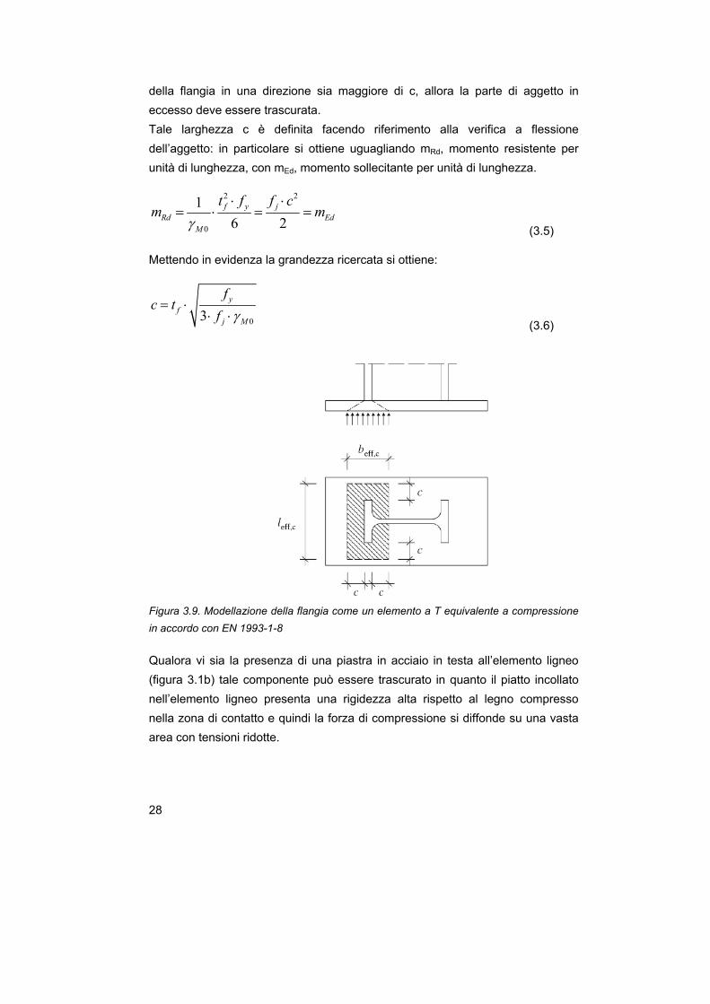
− leff è la larghezza efficace del T-stub. Si assume che gli sforzi di compressione siano uniformemente distribuiti su di un’area rettangolare di lati beff ed leff. Nella definizione di tale superficie di contatto si fa riferimento alla larghezza della zona di contatto c: qualora l’aggetto
28
della flangia in una direzione sia maggiore di c, allora la parte di aggetto in eccesso deve essere trascurata. Tale larghezza c è definita facendo riferimento alla verifica a flessione dell’aggetto: in particolare si ottiene uguagliando mRd, momento resistente per unità di lunghezza, con mEd, momento sollecitante per unità di lunghezza.
2 2
0
16 2
f y jRd Ed
M
t f f cm m
γ⋅ ⋅
= ⋅ = = (3.5)
Mettendo in evidenza la grandezza ricercata si ottiene:
03y
fj M
fc t
f γ= ⋅
⋅ ⋅ (3.6)
Figura 3.9. Modellazione della flangia come un elemento a T equivalente a compressione in accordo con EN 1993-1-8
Qualora vi sia la presenza di una piastra in acciaio in testa all’elemento ligneo (figura 3.1b) tale componente può essere trascurato in quanto il piatto incollato nell’elemento ligneo presenta una rigidezza alta rispetto al legno compresso nella zona di contatto e quindi la forza di compressione si diffonde su una vasta area con tensioni ridotte.
29
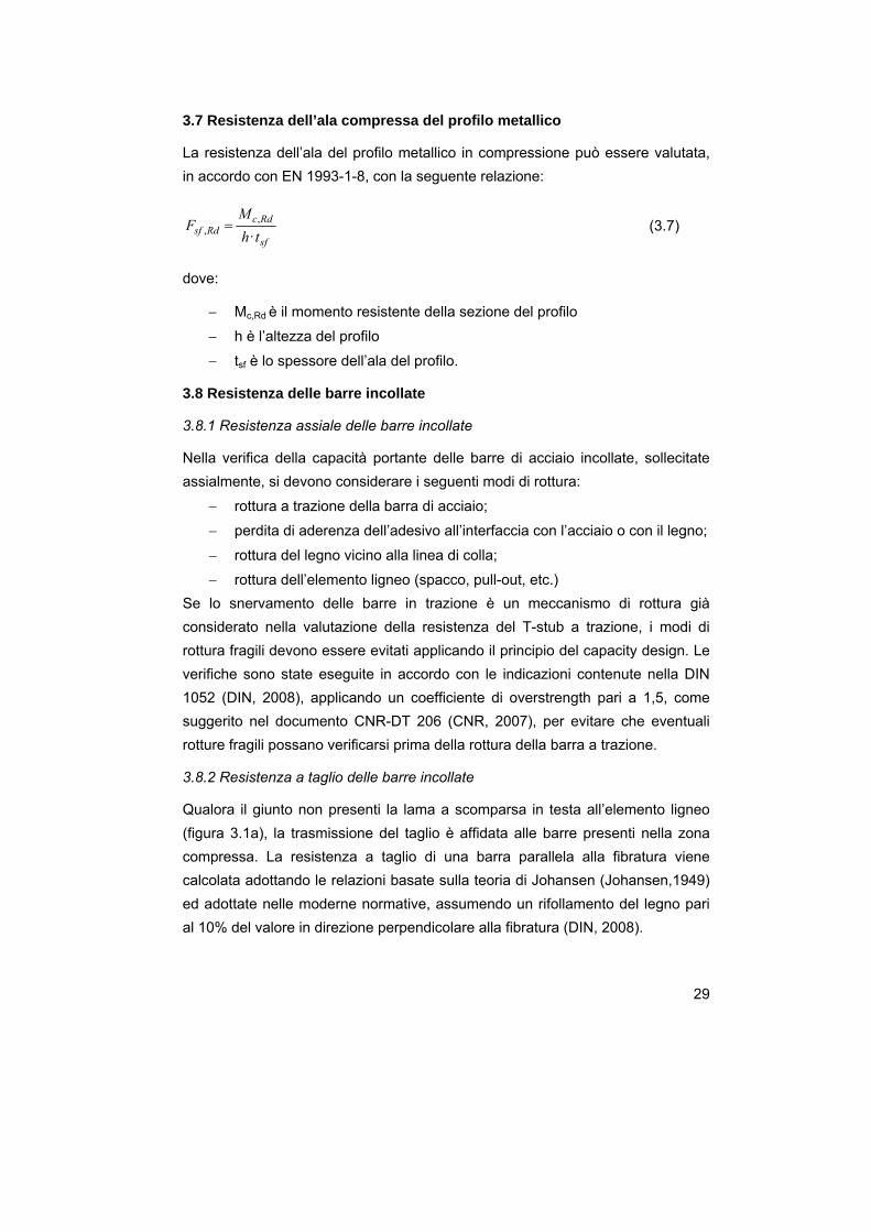
3.7 Resistenza dell’ala compressa del profilo metallico
La resistenza dell’ala del profilo metallico in compressione può essere valutata, in accordo con EN 1993-1-8, con la seguente relazione:
sf
RdcRdsf th
MF
·,
, = (3.7)
dove:
− Mc,Rd è il momento resistente della sezione del profilo
− h è l’altezza del profilo
− tsf è lo spessore dell’ala del profilo.
3.8 Resistenza delle barre incollate
3.8.1 Resistenza assiale delle barre incollate
Nella verifica della capacità portante delle barre di acciaio incollate, sollecitate assialmente, si devono considerare i seguenti modi di rottura:
− rottura a trazione della barra di acciaio;
− perdita di aderenza dell’adesivo all’interfaccia con l’acciaio o con il legno;
− rottura del legno vicino alla linea di colla;
− rottura dell’elemento ligneo (spacco, pull-out, etc.) Se lo snervamento delle barre in trazione è un meccanismo di rottura già considerato nella valutazione della resistenza del T-stub a trazione, i modi di rottura fragili devono essere evitati applicando il principio del capacity design. Le verifiche sono state eseguite in accordo con le indicazioni contenute nella DIN 1052 (DIN, 2008), applicando un coefficiente di overstrength pari a 1,5, come suggerito nel documento CNR-DT 206 (CNR, 2007), per evitare che eventuali rotture fragili possano verificarsi prima della rottura della barra a trazione.
3.8.2 Resistenza a taglio delle barre incollate
Qualora il giunto non presenti la lama a scomparsa in testa all’elemento ligneo (figura 3.1a), la trasmissione del taglio è affidata alle barre presenti nella zona compressa. La resistenza a taglio di una barra parallela alla fibratura viene calcolata adottando le relazioni basate sulla teoria di Johansen (Johansen,1949) ed adottate nelle moderne normative, assumendo un rifollamento del legno pari al 10% del valore in direzione perpendicolare alla fibratura (DIN, 2008).

30
3.9 Valutazione della rigidezza del giunto
La rigidezza rotazionale iniziale Sj,ini può essere determinata in accordo con la relazione proposta da EN 1993-1-8 (CEN, 2005):
∑1
2
,
i
sinij
k
· zES = (3.8)
dove Es è il modulo elastico dell’acciaio e ki è il coefficiente di rigidezza relativo all’i-esimo componente di base (figura 3.10):
− kp è il coefficiente di rigidezza della flangia d’estremità in zona tesa;
− kb è il coefficiente di rigidezza delle barre tese;
− kt è il coefficiente di rigidezza del legno in compressione.
Gli altri componenti di base forniscono un contributo trascurabile alla rigidezza rotazionale del giunto.
Figura 3.10. Modello per il calcolo della rigidezza del giunto
3.10 Rigidezza flangia d’estermità in zona tesa
Il coefficiente kp può essere determinato con le relazioni riportate in EN 1993-1-8 (CEN, 2005):
− in presenza di forze di contatto:
3
3,85,0
m
· t · lk fteff
p = (3.9)

31
− in assenza di forze di contatto:
3
3,425,0
m
· t · lk fteff
p = (3.10)
dove leff,t, tf ed m sono rispettivamente è la lunghezza efficace del T-stub, lo spessore della flangia ed un parametro geometrico del T-stub equivalente in trazione (figura 3.7)
3.11 Rigidezza delle barre tese
3.11.1 Relazioni di calcolo
Il coefficiente kb può essere determinato con le relazioni riportate in EN 1993-1-8 (CEN, 2005):
− in presenza di forze di contatto:
b
sb L
· Ak 6,1= (3.11)
− in assenza di forze di contatto:
b
sb L
· Ak 0,2= (3.12)
dove As è l’area della sezione resistente e Lb è la lunghezza di calcolo della barra filettata, assunta pari alla somma di: α volte il diametro nominale della barra, lo spessore di piastre, rondella e metà dell’altezza del dado.
Figura 3.11. Lunghezza di calcolo della barra incollata

32
3.11.2 Valutazione del parametro α
Nel caso di tirafondi annegati nel calcestruzzo l’EC3 suggerisce di utilizzare un valore di α pari ad 8, mentre nel caso in esame il parametro α può essere valutato applicando la trattazione effettuata da Volkersen per i giunti a semplice sovrapposizione (Volkersen, 1938) al caso di giunti incollati a simmetria assiale come è il caso delle barre incollate (figura 3.12).
σs0
hom
xx
σw
σσs = w
sσ (x) σ
τ(x)
dx
(x)sσ + d s (x)
(x)τ
n
Figura 3.12. Giunto assial-simmetrico con barra incollata
Nel caso assialsimmetrico è possibile scrivere le seguenti quattro equazioni:
• equazione di equilibrio globale in x:
wwssss AxAxA ·)(·)(·0 σσσ += (3.13) • equazione indefinita di equilibrio per l’elemento dx:
dxxAxd ss ·)(···)( _ τπσ Φ= (3.14)

33
• equazione indefinita di congruenza:
s
s
w
wsw E
xE
xxx
dxxds )()(
)()()( __ σσ
εε == (3.15)
• legge costitutiva:
)(·)( xGtxs τ= (3.16)
dove:
− t è lo spessore della linea di colla;
− s è lo spostamento tra gli elementi incollati a livello della linea di colla;
− Φ è il diametro della barra d’acciaio;
− G è il modulo di taglio della linea di colla.
Combinando l’equazione (3.13) con la (3.15) si ottiene:
( )0_
ww
__ss
s
s
s · · EAA
Edxds σσ
σ= (3.17)
Derivando questa equazione si ottiene:
⎥⎦
⎤⎢⎣
⎡+=
ww
s
s
s
· EAA
E ·
dxd
dx
sd 1_2
2 σ (3.18)
Tenendo presente l’equazione (3.14):
s
s
A · ·
dxd τφπσ _= (3.19)
si ottiene:
⎥⎦
⎤⎢⎣
⎡+=
wwss · EA · EA · · ·
dxsd 112
2τφπ (3.20)
Dalla (3.16) si ottiene quindi:
⎥⎦
⎤⎢⎣
⎡+=
wwss EAEAtGx
dxxd 11····)()(
2
2 φπττ (3.21)

34
Adottando le seguenti posizioni:
ww
ss
AEAE
··
=ψ [adimensionale] (3.22)
tAEG
ss ···· φπ
=Γ [1/L2] (3.23)
( )ψω +Γ= 1·2 [1/L2] (3.24)
l’equazione (3.21) può essere riscritta come:
22
2
ωτ=τ
·)x(dx
)x(d (3.25)
Tale equazione fornisce la soluzione:
( ) ( )xAxAx ⋅⋅+⋅⋅= ωωτ sinhcosh)( 21 (3.26)
Combinando le equazioni (3.16) e (3.17) si ottiene:
( )⎥⎦
⎤⎢⎣
⎡−⋅
⋅+⋅−= 0ss
ww
s
s
s
EAA
EtG
dxd σσ
στ (3.27)
Si hanno le seguenti condizioni al contorno:
x = 0 (inizio barra):
sss A
P== 0)0( σσ (3.28)
Sostituendo nella (3.27):
tAEPG
dxd
ss ⋅⋅⋅
−=)0(τ (3.29)
x = xhom:
idws A
Pnnx ⋅=⋅= σσ )( hom (3.30)
dove:
swid AnAA ⋅+= (3.31)

35
w
s
EE
n = (adimensionale) (3.32)
Sostituendo nella (3.27) si ottiene:
0)( hom =xdxdτ (3.33)
Applicando le condizioni al contorno si ottiene quindi:
x = 0 (inizio barra):
( ) ( )[ ]0cosh0sinh 21 ⋅+⋅⋅=⋅⋅
⋅− AA
tAEPG
ssω (3.34)
ml
lPlPA τ
ψω
φπψω
φπω⋅
+⋅
−=⋅⋅
⋅+
⋅−=
⋅⋅⋅Γ
−=)1()1(2 (3.35)
x = xhom:
( ) ( )⎥⎦
⎤⎢⎣
⎡⋅⋅
⋅⋅⋅Γ
−⋅⋅⋅= homhom1 coshsinh0 xPxA ωφπω
ωω (3.36)
Nell'ipotesi di barra sufficientemente lunga si ricava:
mlPA τ
ψω
φπω⋅
+⋅
=⋅⋅
⋅Γ=
)1(1 (3.37)
La soluzione del problema vale quindi:
( ) ( ) ( ) ( ) ( )x
mm elxlxl ⋅−⋅⋅+
⋅=⋅⎥
⎦
⎤⎢⎣
⎡⋅⋅
+⋅
−⋅⋅+
⋅= ωτ
ψωτω
ψωω
ψωτ
1sinh
1cosh
1 (3.38)
L’azione assiale nella barra vale:
( )∫ ⋅⋅⋅−=x
s dxPxP0
)( φπτ (3.39)
Integrando si ottiene:
( ) xxs ePPePPxP ⋅−⋅− ⋅
++⋅
+=−⋅
+−= ωω
ψψψ
ψ 111
1)( (3.40)

36
Si noti che, dalle equazioni (3.22) e (3.32):
w
s
ww
ss
AA
nAEAE
⋅=⋅⋅
=ψ (3.41)
E quindi:
PAAPA
APnP w
ids
ids ⋅
+=⋅⋅=⋅⋅=
ψψψ
1hom, (3.42)
Del resto, nell'ipotesi di barra sufficientemente lunga (ipotesi valida nel caso reale di barre metalliche incollate in elementi in legno):
0hom ≈⋅− xe ω (3.43)
Dall'equazione (3.40) si ha quindi:
hom,hom 1)( ss PPxP =⋅
+=
ψψ (3.44)
Ad una distanza xhom nella barra si ha un'azione assiale pari a Ps,hom. La deformazione della barra vale:
)(1
1)()( ,hom,hom, xeP
AEAEP
AExPx iniss
x
ssss
s
ss
ss εε
ψε ω +=⋅
+⋅
⋅+
⋅=
⋅= ⋅− (3.45)
dove i termini:
ss
ss AE
xP⋅
=)(
hom,ε (3.46)
x
ssinis eP
AEx ⋅−⋅
+⋅
⋅= ω
ψε
11)(, (3.47)
sono rispettivamente la il contributo deformativo della sezione omogeneizzata
(εs,hom) ed il contributo deformativo del tratto iniziale della barra (εs,ini), di cui si può tener conto introducendo una lunghezza equivalente della barra tesa Lb. L'allungamento dovuto a questo contributo vale:
ωψεδ
⋅+⋅
⋅=⋅= ∫ )1(
1)(hom
0,
ss
x
inisini AEPdxx (3.48)

37
τ
Bond stress
Tensile action
Ps
Ps, hom
Strain
ε s
ε hom
P
ε s, ini (x)
x
x
x
homx
homx
homx
Figura 3.13. Distribuzione delle tensioni di taglio, dell’azione assiale e della deformazione nella barra metallica
Dalla definizione di lunghezza equivalente Lb:
ssss
bini AE
PAE
LP⋅
⋅⋅=
⋅⋅
=φαδ (3.49)
Si ottiene quindi, confrontando le equazioni (3.48) e (3.49):
φωψφα
⋅⋅+==
)1(1bL (3.50)
In accordo con la precedente espressione i parametri che influenzano il valore di
α sono: il modulo elastico del legno Ew, il modulo elastico dell'acciaio Es, il
diametro della barra φ, l'area di legno Aw (assunta pari a 36 φ2),lo spessore t e il modulo a taglio G della linea di colla.

38
La figura 3.14 mostra la variabilità del parametro α assumendo t=2 mm e G = 1,5 MPa.
Figura 3.14. Range dei valori del parametro α al variare del diametro della barra
3.12 Rigidezza del legno in compressione
3.12.1 Relazioni di calcolo
Il coefficiente di rigidezza kt può essere determinato con una relazione analoga a quella riportata in EN 1993-1-8 (CEN, 2005) nel caso di calcestruzzo in compressione:
s
ceffceffwt E
lbEk
⋅
⋅⋅=
β,, (3.51)
dove Ew è il modulo elastico del legno, Es è il modulo elastico dell'acciaio, beff,c e leff,c sono le dimensioni efficaci del elemento a T-stub equivalente in compressione (figura 3.9).
3.11.2 Valutazione del parametro β
Per determinare la rigidezza del legno in compressione (compresa la deformabilità della flangia in acciaio nella zona compressa) si adotta lo stesso approccio proposto in (ECCS, 1999) a proposito del calcestruzzo in compressione.

39
La rigidezza di una flangia rigida posta su un semispazio di materiale elastico ed isotropo vale, in accordo con (Richard et al., 1970):
rrzr
z lbGPK ⋅⋅⋅−
== βυδ 1
(3.52)
dove P è la forza applicata, δr la deformazione al di sotto del piatto rigido, br e lr
sono le dimensioni del piatto rigido, G è il modulo di taglio, ν è il modulo di
Poisson e βz è un coefficiente numerico determinabile dall’abaco riportato in figura 3.15.
Figura 3.15. Andamento del βz in funzione delle dimensioni della piastra rigida
Le dimensioni del piatto rigido equivalente br e lr sono calcolate facendo riferimento alla dimensione c, calcolata mediante considerazioni di equilibrio (equazione 3.6). Ripercorrendo il ragionamento proposto in (ECCS, 1999) si può dimostrare infatti che la stima di c mediante l’equazione 3.6 risulta adeguata anche per il calcolo della rigidezza del T-stub in compressione (e non solo per la sua resistenza). Il legno è un materiale ortotropo, tuttavia la relazione (3.52) può, con alcune semplificazioni, essere adottata considerando che nell’elemento ligneo analizzato il carico agisce parallelamente alla fibratura. Si assume un rapporto tra il modulo elastico ed il modulo di taglio pari a:
16=GEw (3.53)

40
e un coefficiente di Poisson pari a:
4,0≈≈≈ LTLR ννν (3.53)
dove L, R, T indicano rispettivamente le direzioni anatomiche longitudinale, radiale e tangenziale. L'equazione (3.52) diventa quindi:
( ) rrzw
z lbEK ⋅⋅−⋅
⋅=
υβ
116 (3.54)
Per definizione del coefficiente kt:
βrrw
stzlbE
EkK⋅⋅
=⋅= (3.55)
E quindi dal confronto tra (3.54) e (3.55), il coefficiente β può essere approssimato ad un valore pari a 4:
( ) 4116≈
−⋅=
zβυβ (3.56)
3.13 Valutazione della capacità rotazionale del giunto
La capacità rotazionale del giunto dipende dalla capacità rotazionale del componente più debole. I modi di rottura del giunto in esame sono associati alla resistenza del T-stub in trazione, mentre il contributo degli elementi in compressione è trascurabile. Per calcolare la rotazione ultima ϕCd il giunto è modellato come illustrato nella figura 3.16, utilizzando la seguente relazione:
istub,-Tt,u,Cd
idδ
φ = (3.57)
dove:
− δu,t,T-stub,i è lo spostamento utlimo del T-stub in trazione
− di è assunto come in figura 3.16

41
Figura 3.16. Modi di rottura e relative capacità di deformazione δu,i, come osservato nella campagna sperimentale: (a) modo 1 (provino P6) con completo snervamento della flangia; (b) modo 2 (provino P10) con rottura delle barre e snervamento della flangia in presenza di forze di contatto; (c) modo 3 (provino P20-sp) con rottura delle barre

42
3.14 Valutazione della capacità deformativa del T-stub in trazione
La capacità deformativa del T-stub in trazione può essere valutata in accordo con le seguenti espressioni (Beg and al., 2004) per i tre modi di collasso:
• modo 1 (snervamento completo della flangia)
2 stub,1-t,Tu, · m · uεδ = (3.58)
dove εu è la deformazione ultima dell'acciaio della flangia e m è un parametro geometrico definito nella figura 3.7
Figura 3.17. Deformazione ultima per il modo 1 (Beg and al., 2004)
• modo 2 (rottura delle barre e snervamento della flangia)
)nm
1( · · L bubstub,2-Tt,u, +ε=δ (3.59)
dove εub è la deformazione ultima delle barre d'acciaio e n è un parametro geometrico definito nella figura 3.7
Figura 3.18. Deformazione ultima per il modo 2 (Beg and al., 2004)

43
• modo 3 (rottura delle barre)
La deformazione è semplicemente l'allungamento delle barre a rottura:
bubstub,3-Tt,u, · L ε=δ (3.60)
3.15 Bibliografia
Beg D., Zupancic E., Vayas I., On the rotation capacity of moment connections, Journal of Constructional Steel Research, 2004, 60, 601–620.
Bodig J., Jayne B. A., Mechanics of wood and wood composites, New York, Van Nostrand Reinhold, 1982
CEN, European Committee for Standardization, Eurocode 3: Design of steel structures - Part 1-8: Design of joints, 2005, EN 1993-1-8.
CEN, European Committee for Standardization, Eurocode 5: Design of timber structures. Part 1-1: General - Common rules and rules for buildings, 2004, EN 1995-1-1.
CNR, National Research Council, Instruction for design, execution and control of timber structures (in Italian), 2007, CNR-DT 206/2007.
DIN Deutsches Institut für Normung, Design of timber structures. General rules and rules for buildings (in German), 2008, DIN 1052.
ECCS European Convention for Constructional Steelwork, member TC 10 Structural Connections, Column Bases in Steel Building Frames, Weynand K., Brussels, BE, 1999, Report ECCS TC10-COST C1.
Jaspart J.P., General report: session on connections, Journal of Constructional Steel Research, 2000, 55, 69-89.
Johansen K.W., Theory of Timber Connections, IABSE - International Association of Bridge and Structural Engineering, Bern, Publication No. 9, 1949, 249–262.
Richart, F., E., Hall, J., R., Woods, R., D., Vibrations of Soils and Foundations, Prentice-Hall, Inc., Engelwood Cliffs, New Jersey, 1970
Tomasi R., Zandonini R., Piazza M., Andreolli M., Ductile End Connections for Glulam Beams, Structural Engineering International, IABSE, 18, No. 3, 2008, 290-296.

44
Volkersen O., Die Nietkraftverteilung in zugbeanspruchten Nietverbindungen mit konstanten Laschenquerschnitten (in German), Luftfahrtvorschung, 15, 1938, 41–47.

45
4. VALIDAZIONE DEL MODELLO ANALITICO MEDIANTE ANALISI SPERIMENTALE
4.1 Descrizione della campagna sperimentale
Sono state condotte 16 prove, 8 monotone e 8 cicliche, su giunti acciaio-legno in scala reale. I campioni testati sono formati da una trave in legno di sezione 120 mm x 240 mm e di lunghezza circa 2500 mm, collegata con una configurazione a mensola al giunto acciaio-legno proposto, il quale è incastrato su un muro di reazione. L’elaborazione dei dati ottenuti dalle prove monotone ha permesso di valutare il valore dello snervamento sulla curva sperimentale, necessario alla definizione della procedura di carico delle prove cicliche in accordo con quanto previsto dalla norma EN 12512 (CEN, 2005).
4.1.1 Geometria dei provini testati
Allo scopo di studiare le caratteristiche meccaniche della connessione, con particolare riguardo alla duttilità e all’influenza delle diverse modalità di rottura sulla capacità rotazionale, i provini sono stati realizzati variando lo spessore tf della flangia da 6 mm a 20 mm (tf = 6 mm, 8 mm, 10 mm, 15 mm,20 mm). La geometria dell’elemento metallico flangiato è illustrata nella figura 4.1.
Figura 4.1. Geometria della flangia del sistema di connessione studiato: provini realizzati con (a) o senza (b) lama incollata a scomparsa sulla testa dell’elemento ligneo (unità: mm)

46
Entrambi gli estremi del profilo metallico (HEB 120) sono saldati a flange d’acciaio: una flangia è collegata alla trave in legno lamellare (classe GL24h) per mezzo di 4 barre metalliche (16 mm di diametro, classe 6.8), una flangia è irrigidita e collegata rigidamente ad un muro di reazione per mezzo di 4 o 6 bulloni (a seconda del provino). Nei provini con lama incollata in testa all’elemento ligneo sono stati realizzati nella flangia dell’elemento metallico 4 fori diametro 18 mm, per permettere il trasferimento del taglio alla lama incollata. Nei provini senza lama, dove il taglio è trasmesso direttamente alle barre incollate, sono stati realizzati 4 fori asolati nella flangia così come illustrato in figura 3.1. Questo accorgimento si è reso necessario per permettere il trasferimento del taglio solo mediante le barre poste in zona compressa ed evitare che vengano caricate a taglio le barre poste in zona tesa, evitando la nascita di stati di trazione ortogonale alla fibra ed evitando quindi premature rotture fragili della connessione.
4.1.2 Materiali dei provini testati
Nella tabella 4.1 è riportata la lista dei provini testati: i provini sono indicati con un numero, che indica lo spessore della flangia in mm, mentre il suffisso “sp” indica l’eventuale presenza della lama interna. Le proprietà meccaniche del materiale con cui sono state realizzate le flange dei provini sono state determinate mediante test a trazione su campioni prelevati dal piatto di acciaio utilizzato.
Provino Acciaio flangia
εu %
fy (MPa)
fu (MPa)
P6-sp 38,5 299,6 377,2
P6
P8-sp 38,6 275,5 367,5
P8
P10-sp 45,9 256,1 374,0
P10
P15-sp 35,7 295,5 383,1
P20-sp 36,4 278,2 400,6
Tabella 4.1. Valori misurati delle caratteristiche meccaniche dell’acciaio utilizzato per la realizzazione delle flange dei provini testati

47
4.1.3 Realizzazione dei provini
La realizzazione dei provini è illustrata nelle figure 4.2 e 4.3. Sulla testa dell’elemento ligneo sono stati realizzati 4 fori di diametro 20 mm, con lunghezza variabile da 50 cm a 100 cm per avere la sufficiente lunghezza di incollaggio delle barre metalliche, e le fresature per l’alloggiamento delle lame interne (ove previste).
Figura 4.2. Provino senza lama interna: (a) colatura della resina nei fori (b) inserimento di una barra (c) rimozione della colla in eccesso (d) utilizzo di una dima per il posizionamento delle barre (si noti che la testa delle barre è protetta per evitare che il filetto si sporchi di resina)

48
Figura 4.3. Provino con lama interna: (a) colatura della resina nella fresatura per l’alloggiamento della lama interna (b) inserimento della lama (c) rimozione della colla in eccesso (d) lama posizionata all’interno della fresatura
Operazione molto delicata è l’incollaggio delle barre: la resina bicomponente, una volta miscelata, è colata nei fori della trave e quindi sono inserite ad una ad una le barre filettate, rimuovendo la colla in eccesso. Per garantire un corretto centraggio delle barre nei fori si utilizza una dima. Nel caso del posizionamento delle lame a scomparsa si procede in modo analogo: in questo caso è la lama stessa a fungere da dima per le barre.
4.2 Set-up e protocollo di prova
4.2.1 Set-up di prova
Il set-up di prova progettato consente di avere sul giunto sia flessione che taglio ed è stato utilizzato per i test sia monotoni che ciclici (figura 4.4). E’ stata adottata una configurazione a mensola in cui l’elemento metallico flangiato è rigidamente collegato ad un muro di reazione, mentre il carico è applicato con un attuatore idraulico con un braccio di 2 metri rispetto al giunto indagato, per mezzo di una cerniera perfetta (figura 4.7).
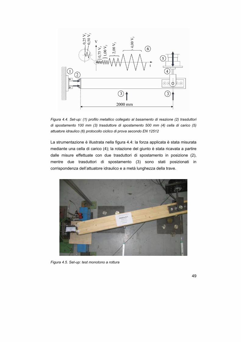
49
Figura 4.4. Set-up: (1) profilo metallico collegato al basamento di reazione (2) trasduttori di spostamento 100 mm (3) trasduttore di spostamento 500 mm (4) cella di carico (5) attuatore idraulico (6) protocollo ciclico di prova secondo EN 12512
La strumentazione è illustrata nella figura 4.4: la forza applicata è stata misurata mediante una cella di carico (4); la rotazione del giunto è stata ricavata a partire dalle misure effettuate con due trasduttori di spostamento in posizione (2), mentre due trasduttori di spostamento (3) sono stati posizionati in corrispondenza dell’attuatore idraulico e a metà lunghezza della trave.
Figura 4.5. Set-up: test monotono a rottura

50
Figura 4.6. Set-up: dettaglio del provino P8 a rottura
Figura 4.7. Set-up: particolare dell'attacco dell'attuatore al provino
4.2.2 Protocollo di prova
Nei test monotoni il carico è stato applicato in controllo di spostamento ad una velocità costante pari a 0,2 mm/sec, raggiungendo la rottura in circa 30 minuti. Il protocollo di prova adottato nei test ciclici è illustrato nella figura 4.4: in accordo con la procedura descritta nella norma europea EN 12512 (CEN, 2005)

51
l’ampiezza dei cicli è definita in funzione del punto di snervamento Vy dei campioni da testare, determinato sperimentalmente dai test monotoni. La velocità di prova è stata aumentata progressivamente per ridurre i tempi secondo i seguenti valori:
− cicli con spostamento non superiore a 0,75 Vy: 0,2 mm/sec
− cicli con spostamento non superiore a 2 Vy: 0,4 mm/sec
− cicli con spostamento superiore: 1,0 mm/sec
Con queste velocità la durata di ogni test ciclico è stata di circa 2 ore. Non tutti i provini hanno raggiunto la rottura a causa del raggiungimento della corsa massima del martinetto pari a +/-250 mm.
4.3 Prove di carico monotone
Nella tabella 4.2 sono indicati per tutti i provini testati monotonicamente: la modalità di rottura, il momento resistente e la capacità rotazionale.
Provino Modo di rottura del T-
stub in trazione Momento resistente
(kNm) Capacità rotazionale
(rad)
Teorico Test Teorico Test * Teorico Test **
P6-sp 1 1 7,08 15,07 0,15 0,20
P6 1 1 6,56 8,85 0,15 0,15
P8-sp 1 2 10,66 16,59 0,16 0,19
P8 1 2 10,51 14,99 0,16 0,21
P10-sp 2 2 15,37 17,14 0,14 0,12
P10 2 2 15,80 19,85 0,13 0,18
P15-sp 2 2 21,82 24,54 0,13 0,14
P20-sp 3 3 28,51 32,29 0,06 0,07
* valore massimo ** rotazione a rottura
Tabella 4.2. Confronto tra il modello teorico e i risultati sperimentali in termini di: modi di rottura del T-stub in trazione, resistenza e rotazione ultima del giunto
Nei paragrafi successivi sono riportate per tutti i provini le curve carico-spostamento sperimentali e il confronto tra le curve momento-rotazione analitiche e sperimentali. I valori teorici sono stati ottenuti utilizzando il modello illustrato nel capitolo 2, assumendo nei calcoli le dimensioni geometriche e le caratteristiche meccaniche dell’acciaio determinate per mezzo di test di trazione (tabella 4.1).

52
Una stima corretta della resistenza ultima dei componenti di base è essenziale per predire correttamente non soltanto la resistenza del giunto, ma anche il tipo di rottura e la capacità rotazionale del giunto. In accordo con quanto suggerito in Beg and al. (2004) nel calcolare la resistenza del T-stub a trazione si è utilizzato il valore della tensione ultima dell’acciaio fu: l’utilizzo della tensione di snervamento come previsto a livello normativo (EN 1993-1-8) conduce a risultati a favore di sicurezza per quanto riguarda la resistenza, ma rischia di non portare all’identificazione corretta del componente più debole, con una conseguente errata identificazione della modalità di rottura e della duttilità del giunto. Si faccia riferimento all’analogia della catena (Paulay e Priestley, 1992) per illustrare il principio della gerarchia delle resistenze: la resistenza di una catena è data dalla resistenza del suo anello più debole e quindi garantendo che questo abbia un comportamento duttile si riesce a fornire duttilità all’intera catena. E’ fondamentale quindi predire correttamente la resistenza dei componenti base del giunto, per evitare modalità di rottura fragili (e.g. pull-out delle barre incollate) e favorire meccanismi di rottura duttili (modo 1 e 2 di rottura del T-stub in trazione). Nessun provino testato ha mostrato rotture fragili (e.g. splitting dovuto a stati di trazione ortogonale alla fibratura). Si è sempre osservata la rottura del T-stub in trazione: in genere con modalità di rottura 1 e 2, tranne per il provino P 20-sp (che presenta il maggior spessore della flangia), che si è rotto con modalità di rottura 3. La tabella 4.2 mostra che il modello analitico proposto è stato in grado di predire la modalità di rottura sperimentale, tranne che per i provini P8-sp e P8, che hanno presentato una rottura di tipo 2, mentre era stata prevista una rottura di tipo 1. Il modello analitico permette inoltre una buona valutazione della capacità di rotazione ultima del giunto, la cui accuratezza è molto legata alla corretta identificazione della modalità di rottura. Si osservi inoltre che nessun provino realizzato senza lama interna ha mostrato rotture legate a stati di trazione ortogonali alla fibratura in seguito alla trasmissione delle forze di taglio per mezzo delle barre metalliche. Il legno è stato inoltre in grado di sopportare le tensioni di contatto con la flangia di acciaio, permettendo la nascita di forze di contatto per il T-stub, conducendo a risultati analoghi in termini di modalità di rottura, momento resistente e capacità di rotazione, rispetto ai corrispondenti provini realizzati con la piastra in testa all’elemento.

53
4.3.1 Test P6-sp
Figura 4.8. Provino P6-sp: curva forza-spostamento sperimentale
Il provino P6-sp ha mostrato una modalità di rottura di tipo 1, con la crisi della cerniera plastica nella flangia in prossimità della saldatura. Avendo raggiunto lo spostamento massimo dell’attuatore non è stato possibile giungere alla rottura completa del campione.
Figura 4.9. Provino P6-sp: (a) deformazione ultima associata a una modalità di rottura tipo 1 (b) crisi della cerniera plastica nella flangia in prossimità della saldatura
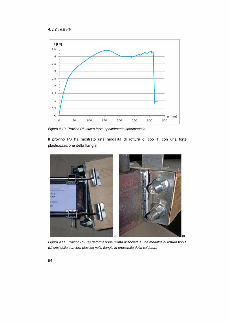
54
4.3.2 Test P6
Figura 4.10. Provino P6: curva forza-spostamento sperimentale
Il provino P6 ha mostrato una modalità di rottura di tipo 1, con una forte plasticizzazione della flangia.
Figura 4.11. Provino P6: (a) deformazione ultima associata a una modalità di rottura tipo 1 (b) crisi della cerniera plastica nella flangia in prossimità della saldatura
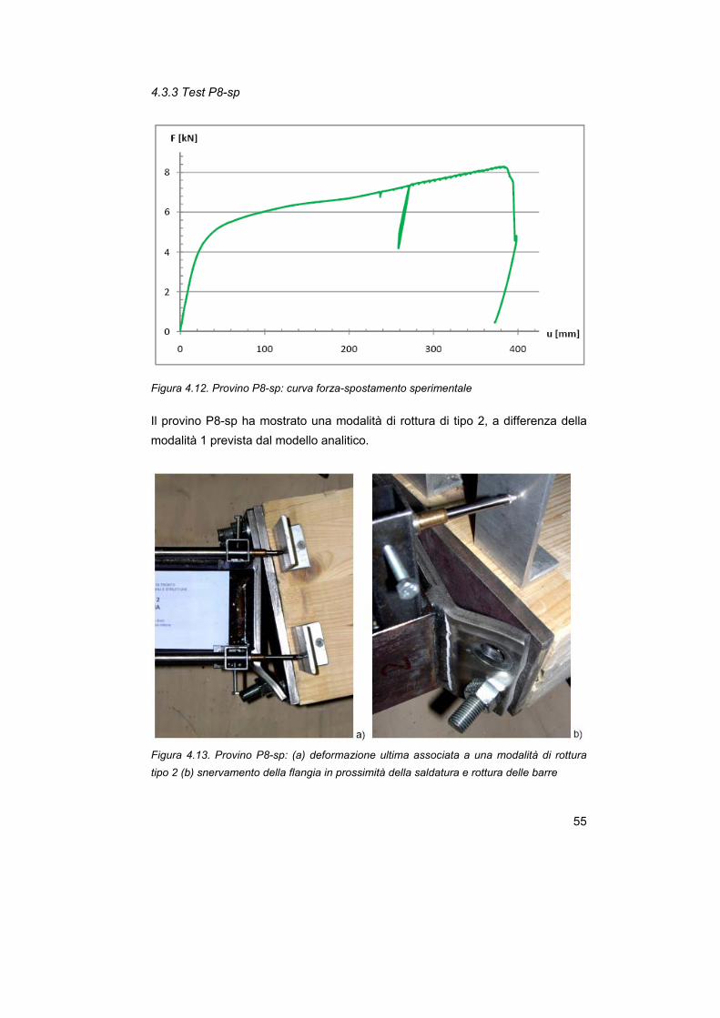
55
4.3.3 Test P8-sp
Figura 4.12. Provino P8-sp: curva forza-spostamento sperimentale
Il provino P8-sp ha mostrato una modalità di rottura di tipo 2, a differenza della modalità 1 prevista dal modello analitico.
Figura 4.13. Provino P8-sp: (a) deformazione ultima associata a una modalità di rottura tipo 2 (b) snervamento della flangia in prossimità della saldatura e rottura delle barre
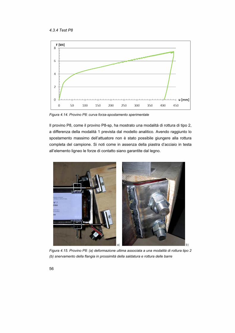
56
4.3.4 Test P8
Figura 4.14. Provino P8: curva forza-spostamento sperimentale
Il provino P8, come il provino P8-sp, ha mostrato una modalità di rottura di tipo 2, a differenza della modalità 1 prevista dal modello analitico. Avendo raggiunto lo spostamento massimo dell’attuatore non è stato possibile giungere alla rottura completa del campione. Si noti come in assenza della piastra d’acciaio in testa all’elemento ligneo le forze di contatto siano garantite dal legno.
Figura 4.15. Provino P8: (a) deformazione ultima associata a una modalità di rottura tipo 2 (b) snervamento della flangia in prossimità della saldatura e rottura delle barre

57
4.3.5 Test P10-sp
Figura 4.16. Provino P10-sp: curva forza-spostamento sperimentale
Il provino P10-sp ha mostrato una modalità di rottura di tipo 2, con la rottura di entrambe le barre metalliche.
Figura 4.17. Provino P10-sp: (a) deformazione ultima associata a una modalità di rottura tipo 2 (b) snervamento della flangia in prossimità della saldatura e rottura delle barre

58
4.3.6 Test P10
Figura 4.18. Provino P10: curva forza-spostamento sperimentale
Il provino P10-sp ha mostrato una modalità di rottura di tipo 2, con la rottura di entrambe le barre metalliche. In assenza della piastra d’acciaio in testa all’elemento ligneo le forze di contatto sono garantite dal legno. Si noti inoltre che a causa delle forti deformazioni le barre metalliche sono soggette ad uno stato di tensoflessione (nonostante l’asolatura dei fori della flangia): non si osservano comunque fessurazioni nel legno dovute a trazione ortogonale alla fibratura.
Figura 4.19. Provino P10: (a) deformazione ultima associata a una modalità di rottura tipo 2 (b) snervamento della flangia in prossimità della saldatura e rottura delle barre

59
4.3.7 Test P15-sp
Figura 4.20. Provino P15-sp: curva forza-spostamento sperimentale
Il provino P15-sp ha mostrato una modalità di rottura di tipo 2. Si noti come la flangia abbia raggiunto una deformazione molto inferiore rispetto ai provini precedenti.
Figura 4.21. Provino P15-sp: (a) deformazione ultima associata a una modalità di rottura tipo 2 (b) snervamento della flangia in prossimità della saldatura e rottura delle barre

60
4.3.8 Test P20-sp
Figura 4.22. Provino P20-sp: curva forza-spostamento sperimentale
Il provino P20-sp ha mostrato una modalità di rottura di tipo 3 con la rottura di entrambe le barre in assenza dello snervamento della flangia.
Figura 4.23. Provino P20-sp: (a) deformazione ultima associata a una modalità di rottura tipo 3 (b) rottura delle barre

61
4.3.9 Confronto tra le curve carico-spostamento sperimentali
Nella figura seguente sono confrontate le curve carico-spostamento relative alle prove monotone.
Figura 4.24. Curve forza-spostamento sperimentali
Appare chiaro che la resistenza dei provini aumenta con l’aumentare dello spessore delle flange ed è maggiore nel caso dei provini realizzati con piastra in testa all’elemento ligneo (in questo caso si ha un braccio della coppia interna leggermente maggiore). La duttilità statica diminuisce all’aumentare dello spessore delle flange e in particolare è minima nel caso del provino P20-sp, che ha mostrato una modalità di rottura di tipo 3: in questo caso infatti l’unica plasticizzazione che avviene è quella legata allo snervamento delle barre a trazione, mentre la flangia rimane in campo elastico.

62
4.3.10 Confronto tra le curve momento-rotazione analitiche e sperimentali
Si riporta per tutti i provini il confronto tra le curve momento-rotazione analitiche e sperimentali. I valori teorici sono stati ottenuti utilizzando il modello illustrato nel capitolo 2, utilizzando nei calcoli le caratteristiche meccaniche dell’acciaio determinate per mezzo di test di trazione (tabella 3.1).
Figura 4.25. Provino P6-sp: confronto curva momento-rotazione sperimentale e analitica
Figura 4.26. Provino P6: confronto curva momento-rotazione sperimentale e analitica

63
Figura 4.27. Provino P8-sp: confronto curva momento-rotazione sperimentale e analitica
Figura 4.28. Provino P8: confronto curva momento-rotazione sperimentale e analitica

64
Figura 4.29. Provino P10-sp: confronto curva momento-rotazione sperimentale e analitica
Figura 4.30. Provino P10: confronto curva momento-rotazione sperimentale e analitica
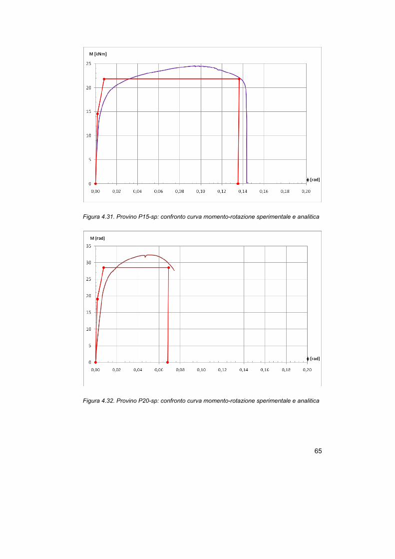
65
Figura 4.31. Provino P15-sp: confronto curva momento-rotazione sperimentale e analitica
Figura 4.32. Provino P20-sp: confronto curva momento-rotazione sperimentale e analitica

66
Come evidenziato nella tabella 4.2 il modello analitico proposto è stato in grado di predire la modalità di rottura sperimentale, tranne che per i provini P8-sp e P8, che hanno presentato una rottura di tipo 2, mentre era stata prevista una rottura di tipo 1. I grafici mostrano come il modello riesca a predire con sufficiente accuratezza le proprietà meccaniche del giunto, sia in termini di rigidezza che di resistenza e rotazione ultima. Nel solo provino P10-sp si nota una rotazione ultima prevista superiore a quella verificata sperimentalmente: ciò è dovuto ad un collasso prematuro delle barre a trazione. La figura 4.33 evidenzia come la rigidezza rotazionale aumenti all’aumentare dello spessore di flangia e in presenza di lama in testa all’elemento ligneo. Interessante notare come la rigidezza iniziale del campione P20-sp, che è l’unico che giunge a collasso nel modo 3, presenta una rigidezza inferiore al campione P15-sp: questo è da imputarsi all’assenza di forze di contatto in testa alla flangia.
Figura 4.33. Confronto curve momento-rotazione sperimentali nel tratto iniziale

67
4.4 Prove di carico cicliche
4.4.1 Protocollo di prova adottato
I test ciclici sono stati condotti in accordo con il protocollo di prova indicato nella norma europea EN 12512 (CEN, 2005), la quale prescrive una serie di cicli ad ampiezza crescente, definiti in funzione del punto di snervamento Vy dei campioni da testare (figura 4.4). Lo scorrimento allo snervamento Vy è stimato dai dati sperimentali ottenuti dalle prove monotone, secondo quando la procedura illustrata in figura 4.34.
Figura 4.34. Definizione del valore di snervamento per una curva carico-spostamento EN 12512 (CEN, 2005)
Nella tabella 4.3 è riportato per ogni provino la determinazione di Vy.
Provino Fmax
[kN] 0,4 Fmax
[kN] 0,1 Fmax
[kN] Fy
[kN] Vy
[mm] P6-sp 8,02 3,21 0,80 3,60 26,7
P6 4,42 1,77 0,44 2,85 29,5
P8-sp 8,29 3,31 0,83 4,43 21,8
P8 7,49 3,00 0,75 3,46 30,2
P10-sp 8,65 3,46 0,86 5,56 29,0
P10 10,00 4,00 1,00 5,62 26,5
P15-sp 12,44 4,97 1,24 8,47 22,85
P20-sp 16,42 6,57 1,64 13,04 46,2
Tabella 4.3. Determinazione del valore di snervamento

68
Nelle figure seguenti si riporta la determinazione grafica di Vy per i diversi provini.
Figura 4.35. Provino P6-sp: definizione del valore di snervamento
Figura 4.36. Provino P6: definizione del valore di snervamento
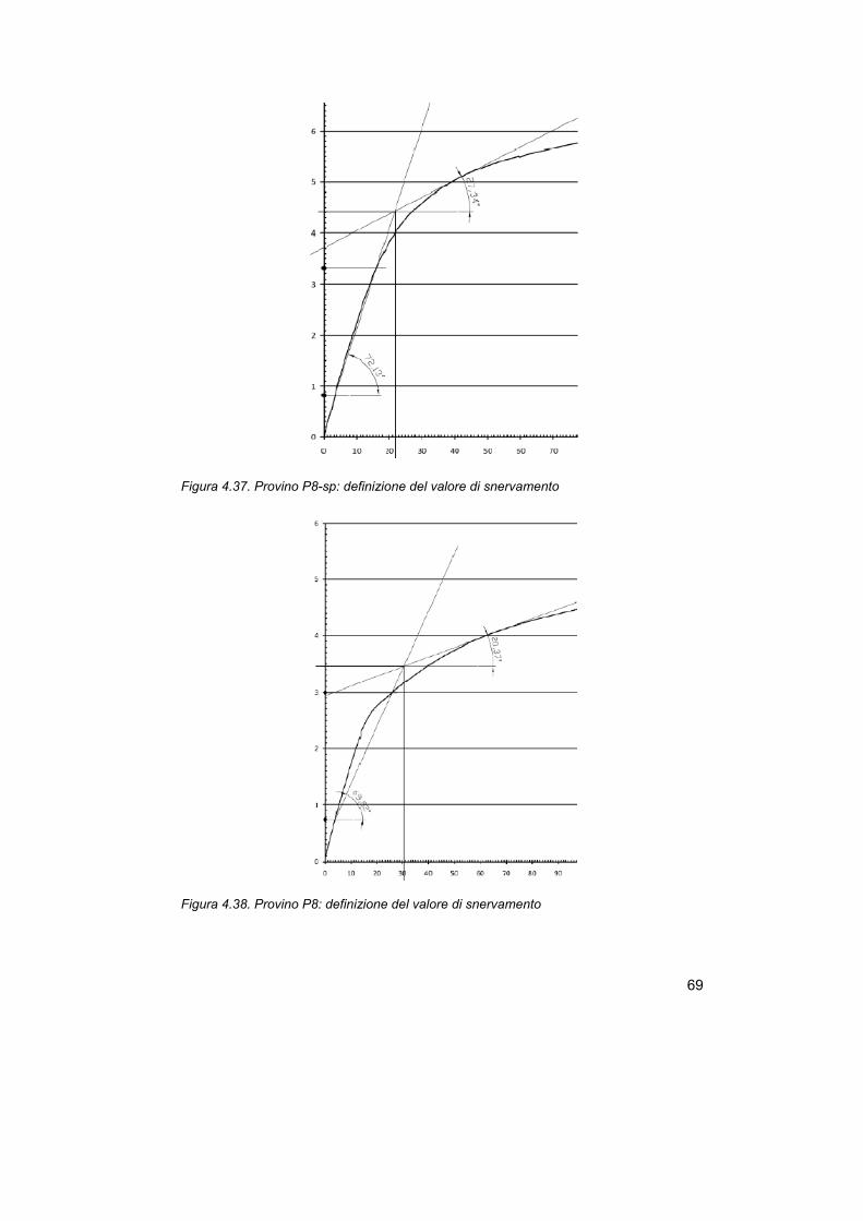
69
Figura 4.37. Provino P8-sp: definizione del valore di snervamento
Figura 4.38. Provino P8: definizione del valore di snervamento

70
Figura 4.39. Provino P10-sp: definizione del valore di snervamento
Figura 4.40. Provino P10: definizione del valore di snervamento

71
Figura 4.41. Provino P15-sp: definizione del valore di snervamento
Figura 4.42. Provino P20-sp: definizione del valore di snervamento

72
4.4.2 Test P6-sp
Il provino P6-sp ha presentato la rottura della flangia durante il terzo sub-ciclo del ciclo “8Vy”.
0,25 Vy
[mm] 0,5 Vy
[mm] 0,75 Vy
[mm] Vy
[mm] 2 Vy
[mm] 4 Vy
[mm] 6 Vy
[mm] 8 Vy
[mm] 6,75 13,5 20,25 27,0 54,0 108,0 162,0 216,0
Tabella 4.4. Provino P6-sp: valori di spostamento imposti
Figura 4.43. Provino P6-sp: protocollo di prova
Figura 4.44. Provino P6-sp: (a) deformazione ultima (b) crisi della cerniera plastica nella flangia in prossimità della saldatura

73
4.4.3 Test P6
Il provino P6 ha presentato la rottura della flangia durante il terzo sub-ciclo del ciclo “8Vy”, con un comportamento analogo a quello del provino P6-sp.
0,25 Vy
[mm] 0,5 Vy
[mm] 0,75 Vy
[mm] Vy
[mm] 2 Vy
[mm] 4 Vy
[mm] 6 Vy
[mm] 8 Vy
[mm] 7,5 15,0 22,5 30,0 60,0 120,0 180,0 240,0
Tabella 4.5. Provino P6: valori di spostamento imposti
Figura 4.45. Provino P6: protocollo di prova
Figura 4.46. Provino P6: (a) deformazione ultima (b) crisi della cerniera plastica nella flangia in prossimità della saldatura

74
4.4.4 Test P8-sp
Il provino P8-sp ha presentato la rottura della flangia durante il terzo sub-ciclo del ciclo “10Vy”.
0,25 Vy
[mm] 0,5 Vy
[mm] 0,75 Vy
[mm] Vy
[mm] 2 Vy
[mm] 4 Vy
[mm] 6 Vy
[mm] 8 Vy
[mm] 10 Vy
[mm] 5,75 11,5 17,25 23,0 46,0 92,0 138,0 184,0 230,0
Tabella 4.6. Provino P8-sp: valori di spostamento imposti
Figura 4.47. Provino P8-sp: protocollo di prova
Figura 4.48. Provino P8-sp: (a) deformazione ultima (b) crisi della cerniera plastica nella flangia in prossimità della saldatura

75
4.4.5 Test P8
Il provino P8 non ha raggiunto la rottura a causa del raggiungimento della corsa massima del martinetto pari a +/-250 mm.
0,25 Vy
[mm] 0,5 Vy
[mm] 0,75 Vy
[mm] Vy
[mm] 2 Vy
[mm] 4 Vy
[mm] 6 Vy
[mm] 8 Vy
[mm] 7,75 15,5 23,25 31,0 62,0 124,0 186,0 248,0
Tabella 4.7. Provino P8: valori di spostamento imposti
Figura 4.49. Provino P8: protocollo di prova
Figura 4.50. Provino P8: (a) deformazione a termine prova (b) cerniera plastica nella flangia in prossimità della saldatura

76
4.4.6 Test P10-sp
Il provino P10-sp non ha raggiunto la rottura a causa del raggiungimento della corsa massima del martinetto pari a +/-250 mm.
0,25 Vy
[mm] 0,5 Vy
[mm] 0,75 Vy
[mm] Vy
[mm] 2 Vy
[mm] 4 Vy
[mm] 6 Vy
[mm] 8 Vy
[mm] 7,25 14,5 21,75 29,0 58,0 116,0 174,0 232,0
Tabella 4.8. Provino P10-sp: valori di spostamento imposti
Figura 4.51. Provino P10-sp: protocollo di prova
Figura 4.52. Provino P10-sp: (a) deformazione a termine prova (b) cerniera plastica nella flangia in prossimità della saldatura

77
4.4.7 Test P10
Il provino P10 non ha raggiunto la rottura a causa del raggiungimento della corsa massima del martinetto pari a +/-250 mm.
0,25 Vy
[mm] 0,5 Vy
[mm] 0,75 Vy
[mm] Vy
[mm] 2 Vy
[mm] 4 Vy
[mm] 6 Vy
[mm] 8 Vy
[mm] 6,62 13,25 19,88 26,5 53,0 106,0 159,0 212,0
Tabella 4.9. Provino P10: valori di spostamento imposti
Figura 4.53. Provino P10: protocollo di prova
Figura 4.54. Provino P10: (a) deformazione a termine prova (b) cerniera plastica nella flangia in prossimità della saldatura

78
4.4.8 Test P15-sp
Il provino P15-sp ha presentato la rottura della flangia alla fine del terzo sub-ciclo del ciclo “8Vy”.
0,25 Vy
[mm] 0,5 Vy
[mm] 0,75 Vy
[mm] Vy
[mm] 2 Vy
[mm] 4 Vy
[mm] 6 Vy
[mm] 8 Vy
[mm] 5,88 11,75 17,62 23,5 47,0 94,0 141,0 188,0
Tabella 4.10. Provino P15-sp: valori di spostamento imposti
Figura 4.55. Provino P15-sp: protocollo di prova
Figura 4.56. Provino P15-sp: (a) deformazione a termine prova (b) crisi della cerniera plastica nella flangia in prossimità della saldatura

79
4.4.9 Test P20-sp
Il provino P20-sp ha presentato la rottura delle barre nel primo sub-ciclo del ciclo “4Vy”.
0,25 Vy
[mm] 0,5 Vy
[mm] 0,75 Vy
[mm] Vy
[mm] 2 Vy
[mm] 4 Vy
[mm] 6 Vy
[mm] 11,75 23,5 35,25 47,0 94,0 188,0 282,0
Tabella 4.11. Provino P20-sp: valori di spostamento imposti
Figura 4.57. Provino P20-sp: protocollo di prova
Figura 4.58. Provino P20-sp: (a) deformazione a termine prova (b) crisi delle barre a trazione

80
4.4.10 Curve momento-rotazione cicliche sperimentali
Si riportano le curve momento-rotazione sperimentali.
Figura 4.59. Provino P6-sp: curve sperimentali momento-rotazione relative ai test monotoni e ciclici
Figura 4.60. Provino P6: curve sperimentali momento-rotazione relative ai test monotoni e ciclici

81
Figura 4.61. Provino P8-sp: curve sperimentali momento-rotazione relative ai test monotoni e ciclici
Figura 4.62. Provino P8: curve sperimentali momento-rotazione relative ai test monotoni e ciclici

82
Figura 4.63. Provino P10-sp: curve sperimentali momento-rotazione relative ai test monotoni e ciclici
Figura 4.64. Provino P10: curve sperimentali momento-rotazione relative ai test monotoni e ciclici

83
Figura 4.65. Provino P15-sp: curve sperimentali momento-rotazione relative ai test monotoni e ciclici
Figura 4.66. Provino P20-sp: curve sperimentali momento-rotazione relative ai test monotoni e ciclici

84
4.4.11 Interpretazione delle prove cicliche
Tutti i provini testati ciclicamente hanno mostrato lo snervamento della flangia metallica tranne il provino P20-sp, dove si è avuta la rottura delle barre a trazione. Si osserva che la frattura nella flangia si è manifestata in seguito ad un alto numero di cicli ad elevati livelli di spostamento in campo plastico. Nell’interpretazione dei dati sperimentali viene seguita la procedura indicata nella norma EN 12512 (CEN,2005). I parametri fondamentali ricavati sono:
• duttilità: definita come il rapporto tra lo spostamento massimo e lo spostamento allo snervamento;
• smorzamento viscoso equivalente νeq: parametro adimensionale che esprime le proprietà di smorzamento per isteresi del giunto, e si misura come il rapporto tra l’energia dissipata in un ciclo e l’energia potenziale disponibile moltiplicata per 2π;
p
deq · E ·
E
π2=ν (4.1)
• diminuzione ∆M/M della resistenza determinata tra il primo e terzo ciclo di uguale ampiezza.
Figura 4.67. Definizioni secondo la norma EN 12512: smorzamento viscoso equivalente νeq e diminuizione della resistenza tra il primo e terzo ciclo di uguale ampiezza
Nelle tabelle 4.12 e 4.13 sono riportati lo smorzamento viscoso equivalente νeq e la diminuzione ∆M/M della resistenza ai diversi valori di spostamento (multipli dello spostamento allo snervamento Vy) raggiunti nei successivi cicli di prova.

85
Provino
νeq (%)
0,75Vy Vy 2 Vy 4 Vy 6 Vy 8 Vy
P6-sp 4,8 8,9 19,7 27,4 26,9 - P6 8,4 12,4 20,3 23,9 22,6 - P8-sp 2,5 6,0 18,3 25,7 27,0 22,7 P8 7,5 13,1 23,1 27,1 28,0 15,2 P10-sp 3,9 6,8 20,0 26,1 27,7 23,9 P10 4,4 9,4 20,5 26,4 28,6 30,2 P15-sp 0,0 0,1 12,6 26,1 33,0 7,9 P20-sp 0,2 0,6 7,4 - - -
Tabella 4.12. Risultati sperimentali delle prove cicliche: smorzamento viscoso equivalente νeq ai diversi valori di spostamento (multipli dello spostamento allo snervamento Vy) raggiunti nei successivi cicli di prova in accordo con la norma EN 12512
Provino
∆M/M (%)
0,75Vy Vy 2 Vy 4 Vy 6 Vy 8 Vy
P6-sp 0,1 0,7 1,5 3,6 23,3 - P6 -1,5 0,8 1,5 5,3 22,3 - P8-sp -0,3 0,6 1,2 3,0 9,2 24,7 P8 -0,8 1,6 1,8 6,1 17,5 36,9 P10-sp -0,1 0,3 2,5 2,6 8,8 16,8 P10 -1,2 1,1 3,0 7,7 10,5 16,6 P15-sp 0,1 0,1 -1,3 3,6 46,2 38,8 P20-sp 0,4 0,6 3,1 - - -
Tabella 4.13. Risultati sperimentali delle prove cicliche: diminuzione ∆M/M della resistenza ai diversi valori di spostamento (multipli dello spostamento allo snervamento Vy) raggiunti nei successivi cicli di prova in accordo con la norma EN 12512
Si noti come i valori di smorzamento viscoso allo snervamento ottenuti siano, per tutti i provini, eccetto che per quelli relativi ai provini P15-sp e P20-sp (provini con gli spessori più elevati delle flange), paragonabili con quelli indicati in letteratura per le strutture metalliche bullonate (Newmark e Hall, 1992). L’Eurocodice 8 (CEN, 2004), in relazione alla definizione del comportamento dissipativo di strutture in legno, indica che “le zone dissipative devono essere in grado di deformarsi plasticamente per almeno tre cicli a inversione completa con un rapporto di duttilità statica pari a 4 per le strutture di classe di duttilità M e con un rapporto di duttilità statica pari a 6 per le strutture di classe di duttilità H, senza che si verifichi una riduzione della loro resistenza maggiore del 20%”.

86
Si nota che tutti i giunti testati, eccetto il provino P20-sp, hanno mostrato la richiesta capacità di deformazione plastica, con valori simili di energia dissipata (νeq = 24-27% per cicli di ampiezza 4 Vy; νeq = 22-33% per cicli di ampiezza 6 Vy). Comunque solo i provini con uno spessore di flangia di 8 e 10 mm presentano una riduzione di resistenza per cicli ad un rapporto di duttilità statica pari a 6 inferiore al 20% e quindi possono essere classificati come altamente dissipativi. Gli altri provini, ad eccezione del P20-sp, sono classificati come a media capacità di dissipazione energetica.
4.5 Bibliografia
Beg D., Zupancic E., Vayas I., On the rotation capacity of moment connections, Journal of Constructional Steel Research, 2004, 60, 601–620.
CEN, European Committee for Standardization, Eurocode 3: Design of steel structures - Part 1-8: Design of joints, 2005, EN 1993-1-8.
CEN, European Committee for Standardization, Eurocode 8: Design of structures for earthquake resistance - Part 1: General rules, seismic actions and rules for buildings, 2004, EN 1998-1.
CEN, European Committee for Standardization, Timber structures. Test methods. Cyclic testing of joints made with mechanical fasteners, 2005, EN 12512.
Newmark N. M., Hall, W.J., Earthquake spectra and design, Earthquake Engineering Research Institute, 1982.
Paulay T., Priestley M.J.N., Seismic design of reinforced concrete and masonry buildings, John Wiley and Sons, 1992.
Longo C., Indagine teorico-sperimentale su giunti flangiati semirigidi in strutture in legno, Tesi di laurea presso l'Università degli Studi di Trento, 2007-2008.
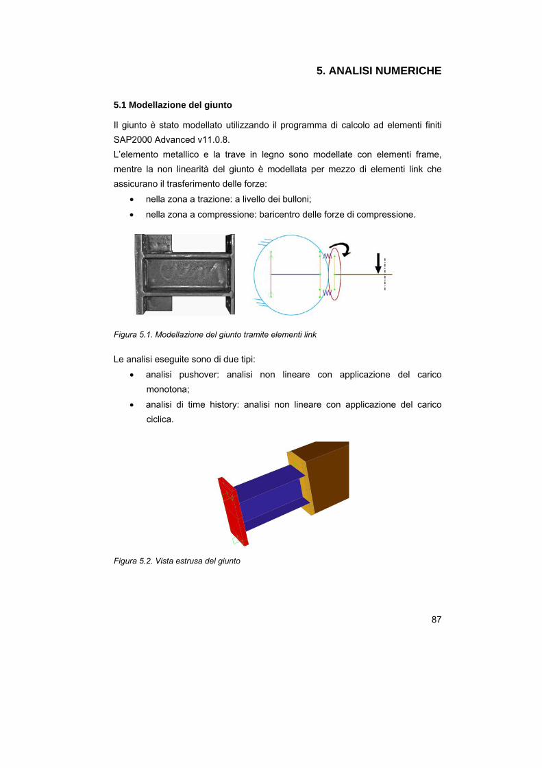
87
5. ANALISI NUMERICHE
5.1 Modellazione del giunto
Il giunto è stato modellato utilizzando il programma di calcolo ad elementi finiti SAP2000 Advanced v11.0.8. L’elemento metallico e la trave in legno sono modellate con elementi frame, mentre la non linearità del giunto è modellata per mezzo di elementi link che assicurano il trasferimento delle forze:
• nella zona a trazione: a livello dei bulloni;
• nella zona a compressione: baricentro delle forze di compressione.
Figura 5.1. Modellazione del giunto tramite elementi link
Le analisi eseguite sono di due tipi:
• analisi pushover: analisi non lineare con applicazione del carico monotona;
• analisi di time history: analisi non lineare con applicazione del carico ciclica.
Figura 5.2. Vista estrusa del giunto

88
5.1.1 Elemento multi-lineare elastico utilizzato nell’analisi pushover
I link sono caratterizzati da :
• deformabilità a taglio nulla: gli elementi trasmettono rigidamente il taglio;
• diagramma forza-spostamento in direzione assiale che modella il comportamento non lineare della connessione.
I diagrammi forza-spostamento sono descritti nelle figure 5.3 e 5.4:
Figura 5.3. Diagramma forza-spostamento del link multi-lineare elastico senza incrudimento
Figura 5.4. Diagramma forza-spostamento del link multi-lineare elastico con incrudimento

89
Figura 5.5. Proprietà dell’elemento link multi-lineare elastico
5.1.2 Elemento multi-lineare plastico utilizzato nell’analisi time hystory
Le proprietà assegnate sono le medesime di quelle previste per il link multi-lineare elastico. I cicli di isteresi sono stati modellati secondo il modello cinematico e secondo il modello di Takeda, molto simile a quello con hardening cinematico ma che presenta un degrado con rigidezza secante una volta passato l’asse in fase di scarico.
Figura 5.6. Proprietà dell’elemento link multi-lineare plastico: (a) ciclo cinematico (b) ciclo di Takeda

90
5.2 Modellazione delle prove
5.2.1 Prove monotone
Si esegue un’analisi statica non lineare in controllo di spostamento, con spostamenti crescenti monotonicamente. Le analisi condotte forniscono risultati in pieno accordo con i risultati ottenuti dalla soluzione analitica. Nella figura 5.7 si mostra, con riferimento al provino P8, un confronto tra le curve sperimentale, analitica e la curva derivante dal modello con SAP2000.
Figura 5.7. Provino P8: confronto tra la curva sperimentale monotona, la curva analitica e la curva derivante dal modello con SAP2000
5.2.2 Prove cicliche
Si esegue un’analisi non lineare con il metodo di integrazione di Newmark assegnando uno spostamento ciclico definito dalla Funzione Time History indicata nella figura 5.8.
Figura 5.8. Definizione della funzione Time History

91
Nella figura 5.9 si mostra, con riferimento al provino P8, un confronto tra la curva ciclica sperimentale e la curva derivante dal modello con SAP2000 (hardening cinematico). Si nota come il modello fornisca risultati accettabili sia in termini di degrado di resistenza che di rotazioni residue, mentre non si riesce a cogliere il degrado di rigidezza nelle fasi di scarico una volta passato l’asse.
Figura 5.9. Provino P8: confronto tra la curva sperimentale ciclica e la curva derivante dal modello con SAP2000
5.3 Caso studio: portale in legno
5.3.1 Descrizione della struttura
Si modella il comportamento di un portale in legno realizzato con i giunti proposti. Il fabbricato ha una pianta rettangolare di dimensioni 15,50 metri x 26,00 metri e presenta una serie di cinque portali disposti ad un interasse di 6,50 metri.

92
Figura 5.10. Caso studio
Rispetto ad una soluzione costruttiva tradizionale quale la realizzazione di portali con nodi d’angolo a raggiera e cerniere alla base, la soluzione con i giunti proposti permette la realizzazione di giunti semi-rigidi anche nell’attacco con la fondazione.
Figura 5.11. Portale ligneo con nodi realizzati con giunti flangiati
Figura 5.12. Dettagli del giunto di base e del giunto trave colonna

93
La geometria delle flange di collegamento del giunto è riportata nella figura 5.13. A differenza dei provini realizzati per i test in laboratorio, si dispongono due file di barre incollate: una fila esterna, da modellarsi con T-stub equivalente a trazione “esterno”, ed una fila interna, da modellarsi con T-stub equivalente a trazione “interno” (figura 5.14), in accordo con le indicazioni riportate nell’eurocodice 3 (CEN, 2005).
Figura 5.13. Geometria del collegamento
Figura 5.14. Geometria del collegamento: T-stub interno (figura centrale) e T-stub esterno (figura a destra)
5.3.2 Descrizione del modello
I giunti sono stati modellati in SAP2000 per mezzo di elementi Link/Support del tipo MultiLinear Elastic come descritto al paragrafo 5.1: elementi Link per collegare due nodi ed elementi Support per collegare un nodo a terra come illustrato schematicamente nelle figure 5.15 e 5.16.

94
Figura 5.15. Modellazione del giunto flangiato di base per mezzo di elementi Link/Support
Figura 5.16. Modellazione del portale per mezzo di elementi Link/Support
5.3.3 Determinazione del fattore di struttura tramite analisi pushover
Obiettivo delle analisi è valutare come cambia il fattore di struttura al variare dello spessore di flangia, stimandolo a partire dalla curva di capacità della struttura. Nella figura 5.17 si illustra la risposta termini di carico-spostamento di una struttura ad un grado di libertà: accanto al comportamento reale sono indicati due schematizzazioni, quella elastica e quella elastica perfettamente plastica. Gli spostamenti ∆1, ∆y e ∆u rappresentano, rispettivamente, lo spostamento della struttura al momento della formazione della prima cerniera plastica, lo spostamento corrispondente alla capacità plastica della struttura idealizzata e lo spostamento ultimo.
GB_cls_sx
GB_leg_sx
TC_tr_sx
TC_pil_sx
TC_tr_dx
TC_pil_dx
GB_leg_dx
GB_cls_dx

95
Figura 5.17. Risposta di un sistema ad un grado di libertà
Si definisce quindi la duttilità come:
u
y
μ Δ=
Δ
(5.1)
Mentre il fattore di struttura q può essere definito come:
1 1
yeu eu
y
VV Vq R RV V V μ Ω= = ⋅ = ⋅
(5.2)
dove:
- euV è il taglio alla base che si avrebbe se il sistema fosse elastico;
- yV
è il taglio alla base dato dallo snervamento del sistema elasto-plastico;
- 1V è il taglio alla base corrispondente alla formazione della prima cerniera plastica.
Il fattore di struttura può essere scomposto quindi nei seguenti fattori parziali:
- il fattore di duttilità Rμ ovvero il rapporto fra il taglio alla base del sistema
elastico a rottura e il taglio alla base del sistema elasto-plastico; - il fattore di sovraresistenza RΩ ovvero il rapporto fra il taglio di
snervamento del sistema elasto-plastico idealizzato e il taglio alla formazione della prima cerniera plastica.
Per quanto riguarda il legame tra il fattore di duttilità e la duttilità per periodi lunghi vale l’ipotesi di uguali spostamenti tra oscillatore elastico ed elasto-plastico e quindi Rµ coincide con μ, mentre nel caso di periodi inferiori vale l’ipotesi di uguale energia e Rµ vale (2μ - 1)0,5.

96
5.3.4 Analisi pushover eseguite
Sono state eseguite analisi di pushover relative alla struttura presentata variando lo spessore delle flange (spessore pari a 6 mm, 10 mm, 16 mm), ottenendo le curve riportate nelle figure seguenti.
Figura 5.18. Portale con flange di spessore 6 mm: curva di pushover
Figura 5.19. Portale con flange di spessore 6 mm: azioni interne ai link

97
Figura 5.20. Portale con flange di spessore 10 mm: curva di pushover
Figura 5.21. Portale con flange di spessore 10 mm: azioni interne ai link

98
Figura 5.22. Portale con flange di spessore 16 mm: curva di pushover
Figura 5.23. Portale con flange di spessore 10 mm: azioni interne ai link

99
5.3.5 Risultati in termini di duttilità e fattore di struttura
A partire dalle curve di capacità si sono costruite le curve bi-lineari del sistema elasto-plastico equivalente imponendo l’equivalenza delle aree sottese. Nella tabella 5.1 sono riportati i risultati delle analisi pushover condotte in termini di:
- F1: forza di base corrispondente al primo snervamento; - Fy: forza di base corrispondente al snervamento del sistema elasto-
plastico equivalente; - ∆y: spostamento di snervamento del sistema elasto-plastico equivalente; - ∆u: spostamento ultimo;
- μ: duttilità;
- Rμ: fattore di duttilità;
- RΩ: fattore di sovraresistenza - q: fattore di struttura
Spessore flangia (mm)
F1 (kN)
Fy (kN)
Δy (mm)
Δu (mm) μ Rμ RΩ q
6 72,14 139,90 26,48 69,95 2,64 2,07 1,94 4,01
10 121,68 226,59 23,59 46,80 1,98 1,72 1,86 3,21
16 155,26 281,98 21,48 30,85 1,44 1,37 1,82 2,48
Tabella 5.1. Risultati delle analisi di pushover in termini di duttilità e fattore di struttura
Si nota che il fattore di struttura decresce all’aumentare dello spessore delle flange: questo è coerente con il fatto che le flange con spessore 6 mm presentano una modalità di rottura di tipo 1 (snervamento completo della flangia), le flange con spessore 10 mm presentano una modalità di rottura di tipo 2 (snervamento della flangia e rottura delle barre incollate), mentre le flange con spessore 16 mm presentano una modalità di rottura di tipo 3 (rottura delle barre a trazione senza lo snervamento della flangia).
5.3.6 Risultati in termini di rigidezza
Nella tabella 5.2 sono riportati i valori di rigidezza iniziale Sini e di rigidezza secante a rottura Ssec della struttura, determinati con riferimento a quanto illustrato nella figura 5.24. Si nota che all’aumentare dello spessore della flangia la rigidezza iniziale, fondamentale per le verifiche in termini di stato limite di esercizio, cresce ma solo in modo molto modesto.
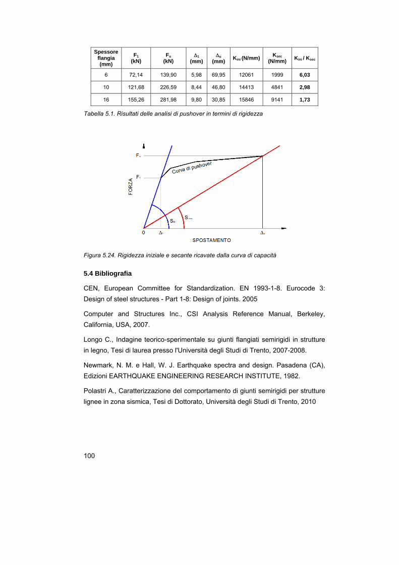
100
Spessore flangia (mm)
F1 (kN)
Fu (kN)
Δ1 (mm)
Δu (mm) Kini (N/mm) Ksec
(N/mm) Kini / Ksec
6 72,14 139,90 5,98 69,95 12061 1999 6,03
10 121,68 226,59 8,44 46,80 14413 4841 2,98
16 155,26 281,98 9,80 30,85 15846 9141 1,73
Tabella 5.1. Risultati delle analisi di pushover in termini di rigidezza
Figura 5.24. Rigidezza iniziale e secante ricavate dalla curva di capacità
5.4 Bibliografia
CEN, European Committee for Standardization. EN 1993-1-8. Eurocode 3: Design of steel structures - Part 1-8: Design of joints. 2005
Computer and Structures Inc., CSI Analysis Reference Manual, Berkeley, California, USA, 2007.
Longo C., Indagine teorico-sperimentale su giunti flangiati semirigidi in strutture in legno, Tesi di laurea presso l'Università degli Studi di Trento, 2007-2008.
Newmark, N. M. e Hall, W. J. Earthquake spectra and design. Pasadena (CA), Edizioni EARTHQUAKE ENGINEERING RESEARCH INSTITUTE, 1982.
Polastri A., Caratterizzazione del comportamento di giunti semirigidi per strutture lignee in zona sismica, Tesi di Dottorato, Università degli Studi di Trento, 2010

101
Schena R., Analisi statica non lineare analisi statica non lineare agli elementi finiti applicata ad un portale iperstatico in legno lamellare con giunti flangiati in acciai, Tesi di laurea presso l'Università degli Studi di Trento, 2007-2008.

102

103
6. CONCLUSIONI E SVILUPPI FUTURI
6.1 Conclusioni
La ricerca presentata è rivolta alla caratterizzazione meccanica di un giunto metallico flangiato da collegare ad elementi lignei mediante barre incollate ed il fissaggio con bullonatura. Questo sistema di connessione presenta diversi interessanti aspetti in termini di: prestazioni meccaniche, in quanto il giunto semi-rigido può essere progettato senza riduzioni significative della resistenza flessionale degli elementi collegati; versatilità, in quanto sono possibili diverse geometrie di giunti resistenti a momento (e.g. giunti d’angolo e alla base di portali come illustrato nella figura 1.1); alto livello di prefabbricazione, in quanto il montaggio della struttura può avvenire mediante bullonatura come in una costruzione metallica, riducendo i tempi di realizzazione e le operazioni da eseguirsi in cantiere. Diversi autori hanno proposto e studiato in passato configurazioni simili di giunti con barre incollate: un aspetto finora non sufficientemente indagato è la progettazione sismica di giunti resistenti a momento con barre incollate e la valutazione delle capacità rotazionali degli stessi. Scopo della ricerca è lo sviluppo di una metodologia di progetto che permetta di predire in modo affidabile il comportamento meccanico del giunto in termini non solo di resistenza e rigidezza, ma anche di rotazioni ultime. Obiettivo è quindi quello di giungere alla realizzazione di un giunto in grado di giungere a rottura soltanto in seguito all’applicazione di rotazioni considerevoli, preservando l’integrità degli elementi in legno cui è collegato. Il principio del capacity design può essere illustrato attraverso l’analogia della catena descritta in (Paulay e Priestley, 1992) e in figura 6.1: dato che la resistenza della catena è quella dell’anello più debole è sufficiente garantire che questo elemento presenti un comportamento duttile per conferire duttilità a livello globale. Nelle strutture in legno la duttilità è concentrata esclusivamente nelle connessioni, mentre gli elementi in legno vanno considerati come elasto-fragili. Risulta fondamentale a tal proposito valutare correttamente capacità rotazionale e sovraresistenza delle connessioni. La modellazione del comportamento flessionale del giunto è stata ottenuta applicando il “metodo per componenti”, originariamente proposto per le strutture in acciaio e adattato al caso in esame: la scomposizione del giunto nei suoi

104
componenti base ha permesso di progettare la duttilità della connessione,permettendo di predire la modalità di collasso.
Figura 6.1. Illustrazione del principio del capacity design per portali in legno in accordo con l’analogia dell’anello debole di una catena
I risultati delle prove monotone condotte su provini caratterizzati da spessore di flangia variabile indicano un sostanziale accordo tra i risultati teorici e sperimentali in termini di resistenza, modalità di rottura e capacità rotazionale. Le analisi condotte rappresentano un primo passo verso l’utilizzo del giunto proposto in strutture lignee intelaiate in zona sismica. Allo scopo di ottenere l’attivazione di un comportamento duttile del giunto e quindi della struttura in cui è inserito, il principio della gerarchia delle resistenze deve essere applicato così da favorire le modalità di rottura 1 e 2 del T-stub equivalente in trazione (modalità di rottura in cui si ha la deformazione plastica della flangia) e da evitare la modalità di rottura 3 (modalità di rottura in cui la flangia rimane in campo elastico mentre si ha lo snervamento delle barre incollate), in quanto inadeguata a garantire una sufficiente rotazione plastica. I risultati delle prove cicliche hanno confermato l’alta capacità dissipativa di giunti progettati al fine di ottenere modalità di rottura 1 e 2 del T-stub in trazione (nel caso in esame i provini con spessore della flangia variabile da 6 a 15 mm), mentre il provino P20-sp, caratterizzato da una rottura di tipo 3, ha mostrato un comportamento abbastanza fragile. La modellazione numerica non lineare ha permesso inoltre di valutare, con riferimento ad un caso studio di un portale ligneo, il fattore di struttura relativo a strutture realizzate con giunti caratterizzati da un diverso spessore delle flange, ottenendo, per le modalità di rottura dei nodi più duttili, valori paragonabili a quelli di analoghe costruzioni in acciaio. Tali analisi ad elementi finiti hanno confermato come le riserve di duttilità globali siano fortemente influenzate dalla capacità

105
rotazionale dei nodi: di qui la necessità di stabilire regole di progettazione e prescrizioni costruttive qualora si vogliano realizzare costruzioni dotate di alta capacità dissipativa.
6.2 Sviluppi futuri
Futuri sviluppi di indagine riguardano la progettazione ed analisi ad elementi finiti di telai multipiano realizzati con i giunti proposti (figura 6.2). La possibilità di progettare ogni flangia alla resistenza desiderata consente di rispettare il criterio della gerarchia delle resistenze, forzando la plasticizzazione all’estremità delle travi (colonna forte e trave debole). Obiettivo è quindi la progettazione di edifici intelaiati in legno lamellare con giunti a momento in grado di resistere a sollecitazioni cicliche, in grado di esibire un buon comportamento duttile. Si osservi come le strutture intelaiate pesanti stiano assumendo un’importanza sempre maggiore nelle costruzioni in legno: permettono infatti di realizzare ampi spazi non interrotti da setti, con una flessibilità d’uso elevata adatta non solo all’edilizia residenziale, ma anche a spazi commerciali o espositivi.
Figura 6.2. Configurazioni in telai multipiano per il giunto proposto

106

107
APPENDICE A
Tomasi R., Zandonini R., Piazza M., Andreolli M., “A ductile approach design of glued laminated timber structures”, Third International Conference on Structural Engineering, Mechanics and Computation (SEMC 2007), 10-12 September 2007, Cape Town, South Africa

108

109
A ductile approach design of glued laminated timber structures
Summary
Wood is a brittle material, with a poor attitude to dissipate energy: this fact, when comparing timber with other building materials such as steel or reinforced concrete, is a severe obstacle in using timber when ductility is required, mainly in seismic areas, because failure can occur without any warning. The research described in the paper represents an effort to find a “material-adapted” technology to manufacture timber elements and timber joints with an inherent ductility. The first step aims to the investigation on different technological approaches to “pseudo–ductile” elements in timber structures, i.e. by means of the strengthening of the tension side of timber beams. The second phase of the research has been devoted to the investigation of an innovative steel-to-timber joint suitable for different frame joint configurations, where a timber beam is connected to an end plate of a steel stub by means of glued–in steel rods. Both the proposed techniques have been investigated by means of numerical models and experimental tests, in order to determine strength values and moment-curvature relationship of the beam and joints in the plastic field up to failure. Some interesting conclusions can be drawn from the experimental tests, suggesting a possible full implementation of such techniques in seismic resistant timber structures, which is the final goal of this research study.
Keywords
Ductility, glued-in bars, steel-to-timber joints, component method, capacity design.
1. Introduction
The study reported in this paper aims to identify and implement means to improve the dissipative behavior of timber structures, particularly when brittle behavior of wooden elements can represent an obstacle to the choice of timber structures. The research of “material adapted” technologies, endowed with an inherent ductility, has been focused both in the timber elements and in the continuity joints. The basic assumption in designing ductile timber elements is the strengthening of the tension side of the beam, in order to allow the compression side to develop

110
a “plastic” behavior before the brittle failure occurs in the tension zone. This phenomenon can be exploited only with one load direction; the global behavior of these beams has been hence indicated by the authors as “pseudo-ductile”. Different solutions have been already proposed by several authors, in which the tension zones of the timber elements are reinforced, externally or internally, by means of other more resistant materials in order to improve the global stiffness and strength properties of timber beams. Steel re-bars have been used by Lantos (1970). In recent years, the advances of the fiber-reinforced polymer materials industry have encouraged several researchers in the application of FRPs for strengthening timber structures (Gentile and Svecova, 2002). Besides new solution technology, analogous to the reinforced concrete with steel re–bars, with the commercial name Armalam®, were proposed, and attained a patent in Europe. There are few examples, in the scientific literature, of investigations of the failure behavior of wooden beams in bending, accounting for the brittle behavior of fibers in tension. Buchanan (1990) has investigated the possible failure modes of lumber beams, suggesting numerical models in order to study the moment-curvature diagram. Krueger et al. (1974) tried to experimentally verify the feasibility of a limit design approach for “reinforced” wood structures, investigating the possibility of a ductile bending failure of elements (solid wood and glued laminated beams) reinforced by means of steel plates. Because the difficulty to obtain energy dissipation in timber elements, traditionally some structural ductility was achieved via plastic deformations occurring in the metallic joints manufactured with mechanical connectors (dowel, nail, etc.). In timber structures forces between members are in most cases transferred by mechanical dowel type fasteners (drift pins, bars, screws and nails). In these cases the mechanical behavior is correctly described by a general approach, which was firstly proposed by Johansen (1949), and currently adopted by several international standards (e.g. EN 1995 and DIN 1052). Johansen model for dowel type connectors is based on the limit analysis of the joint, which takes into account an ideal plastic behavior of the components. It doesn’t provide any information on some other important aspect, such as the possibility of the occurrence of brittle mechanisms, the elastic properties of the joint (which are important in order to classify kinematically the joint, as pinned or fixed), and the actual displacement capacity of the joint beyond the elastic phase. Several effort have been made in recent years in order to improve the knowledge of these
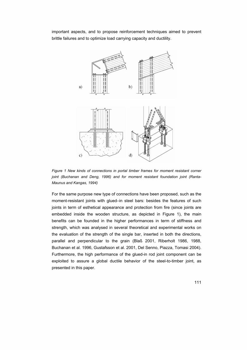
111
important aspects, and to propose reinforcement techniques aimed to prevent brittle failures and to optimize load carrying capacity and ductility.
Figure 1 New kinds of connections in portal timber frames for moment resistant corner joint (Buchanan and Deng, 1996) and for moment resistant foundation joint (Ranta-Maunus and Kangas, 1994)
For the same purpose new type of connections have been proposed, such as the moment-resistant joints with glued–in steel bars: besides the features of such joints in term of esthetical appearance and protection from fire (since joints are embedded inside the wooden structure, as depicted in Figure 1), the main benefits can be founded in the higher performances in term of stiffness and strength, which was analysed in several theoretical and experimental works on the evaluation of the strength of the single bar, inserted in both the directions, parallel and perpendicular to the grain (Blaß 2001, Riberholt 1986, 1988, Buchanan et al. 1996, Gustafsson et al. 2001, Del Senno, Piazza, Tomasi 2004). Furthermore, the high performance of the glued-in rod joint component can be exploited to assure a global ductile behavior of the steel-to-timber joint, as presented in this paper.

112
2. Experimental behavior of steel reinforced glulam beam
2.1 Numerical model
In this paper the non-linear behavior of steel reinforced glued laminated timber beams subjected to simple bending action is studied through an analytical method whose basic assumptions are: 1) the cross-sections remain plane in bending; 2) there is no slip between wood and steel bars; 3) the stress-strain relationship is known both for wood in tension (linear elastic behavior up to failure), and for wood in compression (non-linear plastic behavior). According to the third assumption, different material models were adopted for the wood in compression: I) a linear elastic-perfectly plastic stress-strain relationship; II) a bilinear relationship with a softening branch (Bazan, 1980); III) a general stress-strain relationship reported in literature (O’Halloran, 1973). According to a preliminary experimental validation of wood behavior in compression, the Bazan model has been proved to best fit the experimental data, and therefore was implemented in the numerical model. Two different assumptions were considered for the wood properties in tension: a) linear elastic behavior up to brittle failure; b) no resistant capacity of wood in tension. In the first hypothesis, experimental data for spruce wood failure in tension have been adopted. The second hypothesis, which is not consistent with wood behavior in tension, is usually considered to model steel reinforced concrete beam.
The non-linear pattern of the M-χ relationship of the beam cross-section has been therefore computed incrementally applying a prescribed curvature to the
section, starting from χ0 = 0. For a given curvature, the strains in the section have been evaluated starting from an assumed position of the neutral axis. From the evaluated strain values, the corresponding stresses in wood can be worked out according to the previously assumed stress-strain relationship. The equilibrium check along the beam axis allows then to adjust the position of the neutral axis. Finally, the resisting bending moment can be evaluated by means of the equilibrium condition around, for instance, the neutral axis. The procedure
can be iterated for different couples of values (χ, M), until the condition
⎜ε ⎜ < ⎜εultimate ⎜ is satisfied for both wood, in compression and in tension, and steel.

113
2.2 Experimental analysis
Two differently steel reinforced glulam beams have been designed (figure 2). The
beam indicated as AR2+2 was reinforced by means of Φ 12 mm bars in order to achieve a balanced type of failure, with plastic deformation in the compression zone and yielding of the bars; in the beam indicated as AR1+1+2 some notches had been machined in the tension zone of the wood, in order to artificially reproduce the cracking of the brittle material, as it happens in a steel reinforced concrete beam, and to allow plastic deformation in the bars. Moreover, a third “regular glulam” specimen with the same cross section, in the following referred to as LL 330, has been tested as the reference beam.
Figure 2 Tested pseudo-ductile behaving sections (AR 2+2 left, AR 1+1+2 right)
Figure 3 A steel reinforced timber beam, with the measuring set-up, utilizing the LVDT transducers.

114
2.3 Results and conclusions
The experimental analysis aimed to verify, for both the analyzed techniques, the possibility of a ductile bending behavior. The following parameters have been considered in order to describe in terms of plastic deformation and strength, the failure behavior of the element:
− curvature ductility ( eu χχμχ /= )
− displacement ductility ( eu δδμ χ /= )
− modulus of rupture ( WMMOR u /= )
where:
− χu, χe ultimate bending and elastic bending;
− δu, δu ultimate deflection and elastic deflection;
− W section failure modulus.
0
0,5
1
1,5
2
2,5
3
3,5
4
4,5
LL330 AR2+2 AR1+1+2
Duc
tility
0
10
20
30
40
50
60
70
MO
R
curvature ductility displacement ductility MOR
Armalam® beams 120x165x3300 mm3
0
5
10
15
20
25
30
35
0 0,00005 0,0001 0,00015 0,0002 0,00025
curvature 1/r (1/mm)
Ben
ding
mom
ent (
kNm
)
AR2+2 experimental
AR2+2 numerical
LL330 numerical
AR1+1+2 notches experimental
AR1+1+2 notches numerical
Figure 4 Test results on reinforced timber elements

115
The test results (see the diagrams reported in fig. 4), lead to the following conclusions:
− the reinforced glulam beam, referred to as AR2+2φ12, has shown poor ductile behavior, since the fibre shear failures did not allow the reinforcing bars to reach plasticization;
− the notched reinforced glulam beam, referred to as AR1+1+2φ12, has shown a very high ductile performance as it was foreseen by the numerical model, based on the unrealistic hypothesis of non tension resisting material. A better ductility, however, was obtained thank to a reduction of the beam strength and stiffness.
3. Behavior of steel to timber connections
3.1 End plate joint in steel – timber structures
Taking into account the comprehensive knowledge of this subject, both in terms of scientific results and standard recommendations, it is possible to conceive several different joint configurations where the high resistance capacity of the single glued steel rod can be adequately exploited, like those depicted in figure 1, in order to favorite the ductile behavior of the end plate. In the present paper the joint depicted in figure 5 is theoretically and experimentally analyzed, where a steel stub is connected to a reinforced timber element by means of steel end-plate elements. The transmission of bending moment is assured by the presence of bars glued in timber elements, while the shear forces are transmitted by means of a glued steel plate inserted in a central slot grooved in timber element end.
Figure 5 The end plate joint in steel-timber structure
3.2 The component method applied to steel-to-timber connections
Traditionally timber connections have been regarded as pinned, with negligible moment resistance and rotational stiffness capacity: on the contrary the joint described in this paper has been conceived to behave as semi-rigid (figure 5). Taking into account the particular conception of the joint, in which the steel

116
components play a fundamental role, most of the work done in the past for semi-rigid joints in steel framework can be adapted in order to carry out a feasible general model. The most powerful approach is the component method. In the timber–steel joint depicted in figure 5 the basic components in the compression zone are: steel section flange in compression; end plate in compression; wood in compression. The basic components in tension zone are: end plate in tension; steel bars in tension; the steel section flange in tension.
Figure 6 The internal force distribution in the joint and the related stiffness model
3.3 Evaluation of bending resistance properties and stiffness properties of the joint
In accordance with the component method, the design moment resistance Mj,Rd can be determined when the weakest component of the joint is identified, thus:
z · F M RdRdj, = (1)
z is the lever arm of the internal couple, and:
}F,F ,F ,min{F F Rdgirod,t,Rdfb,c,Rdstub,- Tc,Rdstub,- Tt,Rd = (2)
where:
− Ft,T -stub,Rd: strength of the equivalent T-stub in tension, adopted to model the basic components steel end plate in bending and steel bars in tension;
− Fc,T -stub,Rd: strength of the equivalent T-stub in compression, adopted to model the basic components timber in compression and steel end plate in bending under the bearing pressure;
− Fc,f b,Rd: strength of the compression zone of the beam;
− Ft,girod,Rd: strength of the glued-in rod in tension.

117
The initial rotational stiffness Sj,ini of the joint should be determined from the stiffness of its basic components, each represented by an elastic stiffness coefficient ki, which can be expressed by the following relationship:
· E · k F iii Δ= (3)
where Fi, ki e Δi are respectively the force, the stiffness coefficient and the elongation of the spring representing the basic component, and E is the steel elastic modulus. The initial rotation of the joint can be expressed by the following relation:
∑∑ ⋅⋅=Δ
=i
i
kEzF
z11
Edφ (4)
The moment M acting on the joint is:
z · F M Edj, = (5)
thus the relation for the initial rotational stiffness reported in EN 1993-1-8 can be evaluated:
∑
⋅=
i
inij
k
zES1
2
, (6)
In order to evaluate the rotational stiffness, the joint is modeled according to figure 6, where:
− k1 is the stiffness coefficient for the steel end plate in tension;
− k2 is the stiffness coefficient for the steel bars in tension;
− k3 is the stiffness coefficient for timber in compression.
The flexibility of the steel end-plate in compression is already considered in evaluation of k3 coefficient. The other basic components have only a modest effect on the rotational stiffness of the joint, and their contribution can be neglected. Strength and stiffness parameters for the basic joints component have been derived according to EN 1993-1-8, taking into account the mechanical properties of the wood in modeling the component behavior.

118
4. Validation of the joint model
4.1 Experimental analysis
Different configuration of the joint depicted in figure 5 has been tested. The list of different specimens named “Px” is reported in table 1, where the figure “x” stands for the thickness in mm of the end plate. The European profile HE 120 B has been adopted: in two cases welded profile corresponding to HE 120 B have been used (P10w and P20w). In all specimen, but P10w, shear resistance of the joint is guaranteed by a glued in steel plated inserted in a groove, as depicted in figure 5. In the P10w specimen, shear resistance is assigned to the steel bars. According to previous experimental work (Gheri, 2001) on glued-in-rods, ductile behavior can be only assured by the yielding of the steel bar, which takes place with large strain. However the adhesive is not able to follow so large strains, a progressive reduction of the glued length takes place, and therefore the joint exhibits brittle failure. In order to avoid this behavior, it can be taken advantage from the possibility to control yield force by means a reduced section of the bar. This possibility has been explored in the joint P20w, where the mode 3 of failure was forecasted by modeling the joint according to EN 1993.
Figure 7 Experimental set-up
In order to have both bending and shear actions on the joint, the test set up adopted is the three point configuration test illustrated in figure 7, where the vertical and lateral displacement have been recorded by means of LVDT transducers.

119
4.2 The theoretical model vs. experimental results
The experimental results, reported in table 1 and in figure 8 in terms of force-displacement diagram, confirm the capacity of the model to predict the mechanical behavior of the joint, in term of the global stiffness, moment resistance and failure modes. Moreover test results demonstrated the possibility to ‘design’ the ductility of the joint, by adopting an appropriate geometry of the components (e.g., of the end-plate) so that the ductile failure mode of the T-stub in tension is ensured.
0
5
10
15
20
25
30
35
40
0 25 50 75 100 125 150 175 200 225 250 275
Displacement (mm)
Load
(kN
)
P20wP18
P14
P10 wP10
P6
Figure 8 Experimental results
Specimen Profile Type of failure
Theorical bending failure (kNm)
Experimental bending failure (kNm)
P6 HEB120 1 5,92 11,29 P10 HEB120 2 13,72 19,79
P10w welded 2* 14,19 22,46
P14 HEB120 2 ** 19,90 25,21
P18 HEB120 2 27,86 35,66
P20w welded 3 32,82 38,91 * tension failure of the bar ** brittle failures of the end plate
Table 1 Experimental tests and results

120
5. Conclusions
The post-elastic behavior of reinforced timber beams subjected to pure bending has been explored. In case of steel bar reinforced timber beams, it has been theoretically and experimentally verified that no ductile behavior in bending can be achieved, because brittle failure phenomena in wood occur before the yielding of the steel bars. Limited “pseudo-ductile” phenomenon can be observed, due to plasticization of wood in compression, but this phenomenon is not reversible, and therefore this is not very useful for a seismic design. More promising results can be found when the ductile behavior is concentrated at the joint level. A new type of steel-to-timber ductile joint has been designed by means of the component method. The experimental results seem to confirm its high potential in terms of local ductility. Moreover, the joint model developed provides a satisfactory approximation of the test results, in particular for the ultimate load capacity, and failures modes. This represents a first promising step towards the design and analysis of whole framed structures, where steel-to-timber joints are located at the critical sections (figure 1).
Acknoledgments
The research is partly financed by the Trentino Government Institution (Italy), through the Research Project named CODULE (Ductile Behavior of Timber). Moreover the authors gratefully acknowledge the Italian Reluis Consortium for partial financial support, within the research program carried out for the “Dipartimento Protezione Civile” (the Italian Agency for Emergency Management).
References
[1] Bazan IM. Ultimate bending strength of timber beams, Thesis presented to Nova Scotia Technical College, Halifax, Nova Scotia, in partial fulfillment of the requirements for the degree of Doctor of Philosophy, 1980.
[2] Blass H. J., Laskewitz B., Glued-in rods for timber structures – GIROD Lehrstuhl für Ingegnieur und Baukonstructionen, Universität Karlsruhe
[3] Blass, H.J. and Schmidt, M., Self-tapping screws as reinforcement perpendicular to the grain in timber connections, Proceedings, RILEM Symposium on Joints in Timber Structures, 2001, Stuttgart

121
[4] Bodig J., Jayne B. A., Mechanics of wood and wood composites, New York, Van Nostrand Reinhold, 1982
[5] Brunner M & Schnüringer M. Towards a future with ductile timber beams. In: Proceeding of 7th World Conference on Timber Engineering WCTE. 2002.
[6] Buchanan A. H., Deng X. J., "Strength of Epoxied Steel Rods in Glulam Timber", Proc. of the I.W.E.C., New Orleans, Louisiana, USA, Vol. 4, 1996, pp. 488-495
[7] Bulleit WM, Sandberg LB & Woods GJ. Steel-Reinforced Glued Laminated Timber. Journal of structural engineering. 1989. 115 (2): 433.
[8] CEN, European Committee for Standardization. EN 1194. Timber structures - Glued laminated timber - Strength classes and determination of characteristic values. 1999.
[9] CEN, European Committee for Standardization. EN 1993-1-8. Eurocode 3: Design of steel structures - Part 1-8: Design of joints. 2005
[10] CEN, European Committee for Standardization. EN 1995-1-1, Eurocode 5: Design of timber structures. Part 1-1: General - Common rules and rules for buildings, 2004
[11] CEN, European Committee for Standardization. EN 408. Timber structures. Structural timber and glued laminated timber. Determination of some physical and mechanical properties. 1995.
[12] Del Senno M, Piazza M & Tomasi R. A pseudo-ductile approach design of glued laminated timber beams. In: Proceedings of the 8th World Conference on Timber Engineering WCTE, Lahti, Finland. 2004.
[13] Del Senno M, Piazza M & Tomasi R. Axial glued-in steel timber joints – experimental and numerical analysis. Holz als Roh- und Werkstoff. 2004. 62: 137–146
[14] DIN Deutsches Institut für Normung e.V., DIN 1052:2004, Design of timber structures. General rules and rules for buildings (in german), 2004
[15] Gentile C., Svecova D. (2002). Timber Beams Strengthened with GFRP Bars: Development and Applications, Journal of Composite for Construction Vol. 6 n.1: 11-20.
[16] Gheri, Ductile behavior and group effect of glued-in steel rods, Rilem Proceedings PRO 22, 333-342, Stuttgart, Germany, 2001
[17] Gioncu V. Framed structures. Ductility and seismic response: General Report. Journal of Constructional Steel Research. 2000. 55: 125-154
122
[18] Gustafsson PJ, Serrano E Glued-in rods for Timber Structures – Development of a calculation Model. Technical report for WP1, Project SMT4_CT97:2199 (GIROD), 2001
[19] Haller, P., Progress in timber joint development and modeling, Proceedings of the 5th World Conference on Timber Engineering, Montreux, Switzerland, August 17-20, 1998, Vol. 1: 337 – 344.
[20] Jaspart J.P. General report: session on connections. Journal of Constructional Steel Research. 2000. 55: 69-89
[21] Johansen, K. W., Theory of timber connections, IABSE (1949) Publication no. 9:249-262
[22] Krueger, G. P. and Eddy, F.M., Jr. (1974), Ultimate-strength design of reinforced timber: Moment-rotation characteristics, Wood Sci., 6(4), 330-344.
[23] Krueger, G. P. and Sandberg, L. B. (1974), Ultimate-strength design of reinforced timber: Evaluation of design parameters, Wood Sci., 6(4), 316-330.
[24] Lantos G. The flexural behavior of Steel Reinforced Laminated Timber Beams. Wood Science. 1970. 2 (3): 136–143.
[25] Larsen H.J., Jensen J.L. Influence of semi-rigidity of joints on the behavior of timber structures, Progress of Structural Engineering Materials, 2000 No. 2: 267-277
[26] O’Halloran MR. A curvilinear stress-strain model for wood in compression. Ph. D. Diss. at Colorado State University, Fort Collins, Colorado. 1973.
[27] Paulay T., Priestley M.J.N. Seismic design of reinforced concrete and masonry buildings. John Wiley and Sons. 1992
[28] Plevris N & Triantafillou T. FRP-Reinforced Wood ad Structural Material. Journal of Material in Civil Engineering. 2000. 4: 300-317.
[29] Plumier A. General report on local ductility. Journal of Constructional Steel Research. 2000. 55: 91-107
[30] Ranta-Maunus A, Kangas J. Glue-in steel Rods in V-shape. In Proceedings, Pacific Timber Engineering Conference, 1994, Gold Coast Australia 2:778-784
[31] Riberholt H., Glued bolts in glulam – Proposal for CIB Code. CIB-W 18-21- 7-2, Meeting twenty one Praksville, Vancouver Island, 1988, Canada

123
[32] Stehn L., Johansson H., “Ductility Aspects in Nailed Glue Laminated Timber Connection Design”, Journal of Structural Engineering, 2002, Vol. 128, No. 3: 382-389
[33] Tingley DA & Gai C. FRP reinforced glulam performance: a case study of the lighthouse bridge. In: Proceedings of the 5th World Conference on Timber Engineering WCTE, Montreaux, Switzerland. 1998.
[34] Wald F. Semi-rigid Behavior of Civil Engineering Structural Connections, Second State of the Art Workshop, EU Project COST C1, European Commission, Belgium, 1994: 561.
[35] Wald, F., Jaspart, J., Stiffness design of column bases, Journal of Constructional Steel Research, Volume 46, Issues 1-3, April-June 1998, Page 245

124

125
APPENDICE B
Tomasi R., Zandonini R., Piazza M., Andreolli M., "Ductile End Connections for Glulam Beams", Structural Engineering International, v. 18, n. 3, 2008, p. 290-296

126

127
Ductile End Connections for Glulam Beams
Summary
Ductility, which is the capability of the structure to deform significantly beyond the elastic limit without brittle failure, is a fundamental property which can be an important requirement in many instances. In particular, the behaviour of structures under seismic actions depends on the capacity to withstand large displacements in the plastic field without reaching the collapse. Wood suffers for the unfavourable material characteristic, which do exhibits no (tension) and limited (compression) post-elastic deformation capacity. Therefore timber structures rely on steel dowel type connections to provide ductility and energy dissipation: in general good performance can be achieved by light timber structures, with a large amount of steel connectors, designed to favour steel yielding as the governing mechanism. For heavy timber structures, because the lower redundancy of the structure, a more “engineered” joint design is needed to ensure a safe performance during seismic events. The research reported in the present paper has been devoted to the investigation of an innovative steel-to-timber joint suitable for different joint configurations within a frame, where a timber element is connected to a steel stub by means of an end-plate and glued-in steel rods. The proposed system has been investigated by means of numerical models and experimental tests, in order to determine strength values and moment-rotation relationships of the joint. Some interesting conclusions can already be drawn from the available experimental tests, suggesting a possible full implementation of such techniques in seismic resistant timber structures, which is the final goal of the research.
Keywords
Timber structures; steel-to-timber joints; glued-in rods; ductility; seismic design; component method; capacity design.
Introduction
Wood is a brittle material, with a poor attitude to dissipate energy: contrary to what happens in properly designed steel or reinforced concrete elements, in timber beams failure can occur suddenly, without any warning.

128
Some degree of ductility in bending can be assured for timber elements exploiting the post-elastic capacity of wood in compression, and has been investigated for reinforced timber beams and glulam beams with combined laminations (Tomasi, 2004). This response is commonly referred to as “pseudo-ductile”, because it is associated with the crushing of wood fibres, and, consequently, does not set in if the load is inverted, as it happens during seismic events. The difficulty to obtain energy dissipation in timber elements prompted the use of design approaches achieving some structural ductility via plastic deformations occurring in metallic joints manufactured with dowel type mechanical connectors (e.g. dowels, nails, screws, and bolts). If an appropriate oligocyclic capacity of the timber joints is guaranteed, even for timber structures the capacity design approach can be considered, as stated in European seismic code (CEN, 2004): dissipative zones shall be regarded as located in joints and connections, whereas the timber members themselves shall be regarded as behaving elastically. In general, better performance can be achieved by light timber structures, highly redundant and statically indeterminate, compared to heavy timber structures, where the possibility to dissipate energy is limited by the lower number of ductile joints. For dowel type connectors, which are the most used fixing system both for light and heavy timber structures, accurate strength predictions models were established and adopted in recent standards, based on the European Yield Model (Johansen, 1949; CEN, 2004; DIN, 2004). However, some important aspects were not addressed properly, such as the possibility of the occurrence of brittle mechanisms, the elastic properties and the actual displacement capacity of the joint beyond the elastic phase. In terms of dissipation capacity, the Eurocode 8 only supplies few geometrical provisions to classify a dowel type joint. Several efforts were made in recent years in order to improve the knowledge of these important aspects, and to develop reinforcement techniques aimed at preventing brittle failures and at optimizing both the load carrying capacity and the ductility (Larsen & Hensen, 2000; Blass & Schmidt, 2001). For the same purpose new connections were proposed, such as the moment-resistant joints with glued–in steel bars (Buchanan & Deng, 1996; Ranta-Maunus & Kangas, 1994) (Fig. 1).

129
Besides the features of such joints in terms of esthetical appearance and protection from fire, since steel bars are embedded inside the timber element, the main benefit can be found in the enhanced performance in term of stiffness and strength, as pointed out in several theoretical and experimental works of the evaluation of the response of the single bar, when inserted in the direction parallel or perpendicular to the grain (Del Senno et al., 2004).
Fig. 1: New kinds of connections in portal timber frames for moment resistant corner joint (Buchanan & Deng, 1996) and for moment resistant foundation joint (Ranta-Maunus & Kangas, 1994)
Furthermore, the high performance of the glued-in rod joint component can be exploited to assure a global ductile behaviour of the steel-to-timber joint, as presented in this paper. The use of this kind of joint should be limited, according to recent standards (DIN, 2004), to structural parts assigned to service classes 1 and 2.
Steel to timber connections
End-plate joint in steel-timber structures
In the joint shown in Fig. 2, which is theoretically and experimentally analyzed in the present paper, a steel profile (4) is connected to a reinforced timber element (5) via end-plate elements. Transfer of the bending moment is assured by the presence of bars glued in the timber elements (3), while the shear forces are transmitted by means of a glued

130
steel plate (1) inserted in a central slot grooved at the end of the timbers element (2). The geometry of the steel connection for the present study is illustrated in Fig. 3.
Fig. 2: The end-plate joint in steel-timber structure analyzed
Fig. 3: Geometry of the end-plate connection (measures in mm)
A comprehensive knowledge was achieved of the subject “glued-in bars in timber structures” and “steel end-plate connections”. Besides, scientific results were implemented in recent standard recommendations, enabling the designer to conceive different joint configurations, where the high resistance capacity of the single glued-in steel rod can be exploited to favour the ductile behaviour of the end-plate connection. Most of the work done in the past for semi-rigid joints in steel framework can be adapted in order to set up a feasible general model. To this aim, the component method (Jaspart, 2000; CEN, 2005) is the most powerful approach. In accordance with this method, the timber-steel joint components in the tension and in the compression zone are illustrated in Fig. 4.

131
Fig. 4: Basic joint components for steel to timber joint analyzed, proposed model for internal force distribution and related stiffness
Evaluation of the joint bending resistance and rotational stiffness
The assumed simplified tri-linear moment-rotation curve of the joint is, according to EN 1993-1-8, fully defined by the moment capacity Mj,Rd and the initial stiffness Sj,ini. In accordance with the component method, the design moment resistance Mj,Rd
can be determined when the weakest component of the joint is identified, thus:
z · F M RdRdj, = (1)
where z is the lever arm of the internal couple, and:
=
FFFF
min F
Rdbar,t,
Rdsf,
Rdstub,- Tc,
Rdstub,- Tt,
Rd (2)
where:

132
i. Ft,T -stub,Rd: resistance of the equivalent T-stub in tension, adopted to model the basic components steel end-plate in bending and steel bars in tension;
ii. Fc,T -stub,Rd: resistance of the equivalent T-stub in compression, modelling the basic components, timber and steel end-plate in bending, under compression;
iii. Fsf,Rd: resistance of the steel section flange in compression; iv. Ft,bar,Rd: resistance of the glued-in steel bars in tension (which has been
determined according to the method illustrated in (DIN, 2004), assuming the glued length to be 1 m).
Once the value FRd is computed, the value x which defines the extension of the compression zone (and consequently the lever arm z) can be determined from the translational equilibrium:
ceff,jd
Rd
l ·fF
x = (3)
where fjd and leff,c are the design timber strength for compression parallel to the grain and the effective length of the T-stub flange respectively (see Fig. 4 and Fig. 9). The initial rotational stiffness Sj,ini is a function of the stiffness of the basic joint components. Each individual component is characterized by an elastic stiffness coefficient ki, which can be expressed by the following relationship:
· E · k F isii Δ= (4)
where Es is the elastic modulus of steel, and Fi and ∆i are the force and the elongation of the spring modelling the component respectively. In the elastic field, the moment Mj,Ed acting on the joint is:
z · F · S M Edinij,j,Ed =φ= (5)
The rotation of the joint can be expressed by the following relation:
∑∑ 11
=Δ
=φis
iEd k
· E
· zF
z (6)
Thus the relation for the initial rotational stiffness (CEN, 2005) can be written as:

133
∑1=2
i
sini,j
k
z ·ES (7)
In order to compute the rotational stiffness, the joint is modelled according to Fig. 4, where:
i. kp is the stiffness coefficient for the steel end-plate in bending under tension;
ii. kb is the stiffness coefficient for the steel bars in tension; iii. kt is the stiffness coefficient for timber in compression.
The flexibility of the steel end-plate in compression is already considered in evaluation of kt coefficient, while the other basic components have only a fairly small effect on the rotational stiffness of the joint, and their contribution can be neglected.
Design resistance of basic joint components
i. T-stub in tension. The design resistance and failure mode of the extended end-plate in bending, together with the relevant bars in tension, can be derived, according to EN 1993-1-8, through an equivalent T-stub flange (Fig. 5).
Fig. 5: Modelling an extended end-plate as an equivalent T-stub in tension according to EN 1993-1-8
Four failure modes may be identified (Fig. 6): complete yielding of the flange (mode 1); bars fracture with yielding of the flange (mode 2a); yielding of the

134
flange without prying forces (mode 2b); bars failure (mode 3). In modes 1 and 2a prying forces are present, while in modes 2b and 3 there isn’t contact. Ductility is associated with mode 1 and mode 2.
Fig. 6: Failure modes in a T-stub in tension according to (ECCS, 1999). Mode 1: complete yielding of the flange. Mode 2a: bars failure with yielding of the flange with prying forces. Mode 2b: yielding of the flange without prying forces. Mode 3: bars failure
ii. T-stub in compression. The resistance of the basic components timber and steel end-plate in bending under compression, can be determined through an equivalent T-stub in compression, according to what reported in EN 1993-1-8 for the case of steel column base joints. The ductile failure mode is also associated with this component response.
iii. Resistance of the steel section flange in compression can be determined, according to EN 1993-1-8, by the following expression:
sf
Rd,cRd,sf t ·h
MF = (8)
where Mc,Rd is the design moment resistance of the steel section, h is the depth of the section and tsf is the flange thickness.
iv. Resistance of the glued-in steel bars in tension. Finally, the load-carrying capacity of glued-in axially loaded steel bars should be verified for the following failure modes:
− yielding of the steel bar;
− failure of the adhesive by debonding from steel or wood;
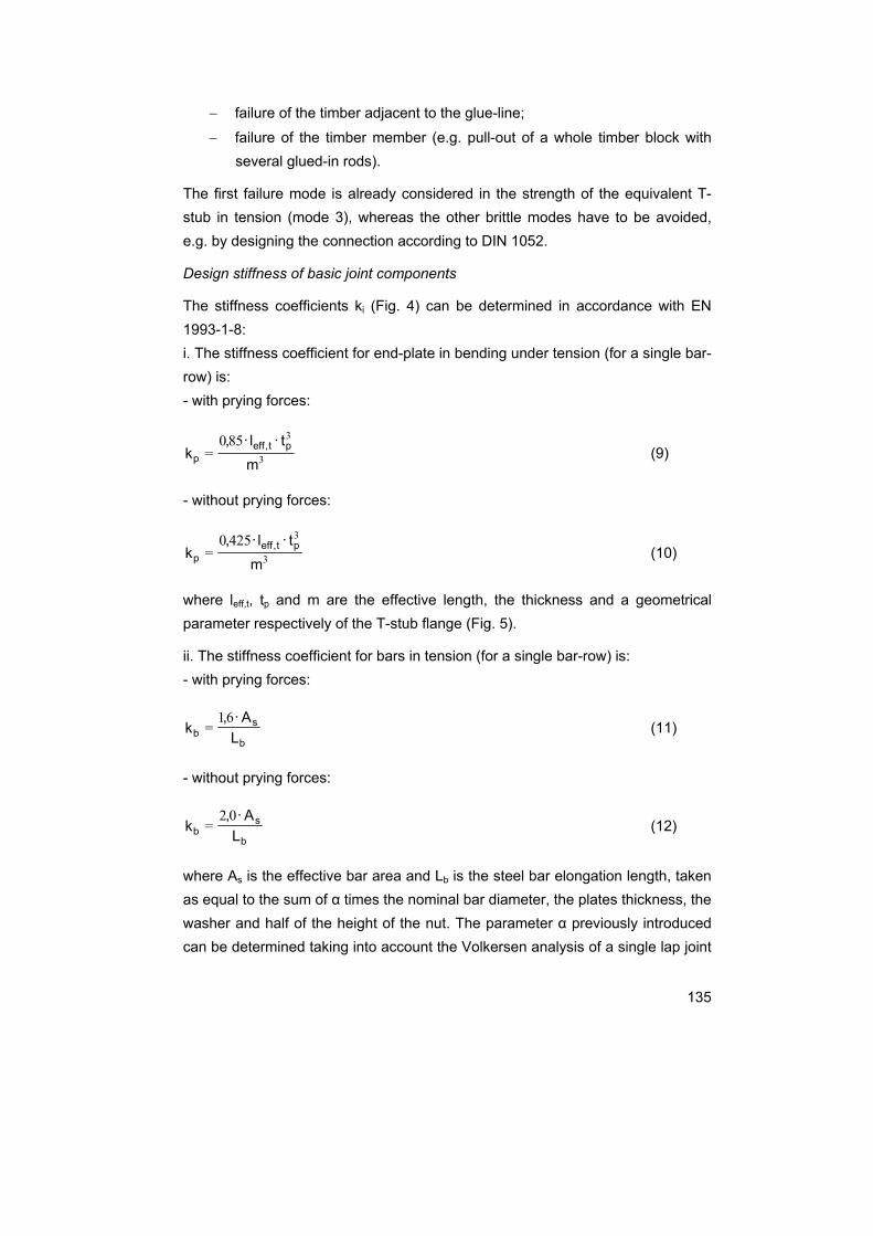
135
− failure of the timber adjacent to the glue-line;
− failure of the timber member (e.g. pull-out of a whole timber block with several glued-in rods).
The first failure mode is already considered in the strength of the equivalent T-stub in tension (mode 3), whereas the other brittle modes have to be avoided, e.g. by designing the connection according to DIN 1052.
Design stiffness of basic joint components
The stiffness coefficients ki (Fig. 4) can be determined in accordance with EN 1993-1-8: i. The stiffness coefficient for end-plate in bending under tension (for a single bar-row) is: - with prying forces:
3
3850=
mt ·l ·,
k pt,effp (9)
- without prying forces:
3
34250=
mt ·l ·,
k pt,effp (10)
where leff,t, tp and m are the effective length, the thickness and a geometrical parameter respectively of the T-stub flange (Fig. 5).
ii. The stiffness coefficient for bars in tension (for a single bar-row) is: - with prying forces:
b
sb L
A ·,k
61= (11)
- without prying forces:
b
sb L
A ·,k
02= (12)
where As is the effective bar area and Lb is the steel bar elongation length, taken as equal to the sum of α times the nominal bar diameter, the plates thickness, the washer and half of the height of the nut. The parameter α previously introduced can be determined taking into account the Volkersen analysis of a single lap joint

136
(Volkersen, 1938). For the case of an axial-symmetric joint (Fig. 7), according to Volkersen, is possible to write the following four equations (global equilibrium in x, indefinite equilibrium for the element dx, indefinite compatibility, constitutive law equation):
wwssss A·)x(A·)x(A· σ+σ=σ 0 (13)
dx·)x(··A·)x(d _ss τΦπ=σ (14)
s
s_
w
ws
_w E
)x(E
)x()x()x(
dx)x(ds σσ
=εε= (15)
)x(·Gt
)x(s τ= (16)
where t is the thickness of the glue line, s is the slip between the adherents at glue line level, Φ is the diameter of the bar, G is the shear modulus of the glue.
Fig. 7: Axial-symmetric joint with a glued-in rod
After few operations it’s possible to obtain the following differential equation:
)1
+1Φπ
τ=τ
2
2
wwss EAEA(·
t··G
·)x(dx
)x(d (17)
Adopting the following positions:
ww
ss
A·EA·E
=ψ [adimensional] (18)
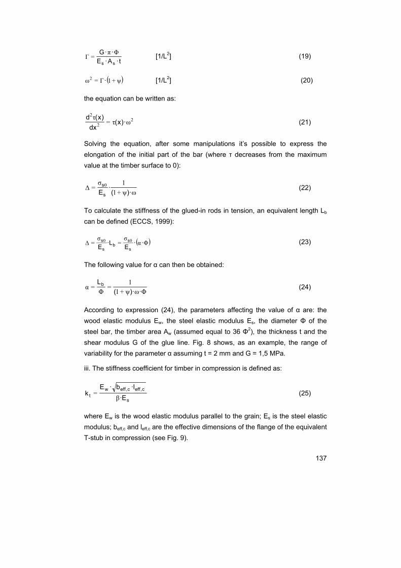
137
t·A·E··Gss
Φπ=Γ [1/L2] (19)
( )ψ+1Γ=ω2 · [1/L2] (20)
the equation can be written as:
22
2
ωτ=τ
·)x(dx
)x(d (21)
Solving the equation, after some manipulations it’s possible to express the elongation of the initial part of the bar (where τ decreases from the maximum value at the timber surface to 0):
ωψ+11σ
=Δ 0
·)(·
Es
s (22)
To calculate the stiffness of the glued-in rods in tension, an equivalent length Lb can be defined (ECCS, 1999):
( )Φασ
=σ
=Δ 00 ··E
L·E s
sb
s
s (23)
The following value for α can then be obtained:
Φωψ+11
=Φ
=α··)(
Lb (24)
According to expression (24), the parameters affecting the value of α are: the wood elastic modulus Ew, the steel elastic modulus Es, the diameter Φ of the steel bar, the timber area Aw (assumed equal to 36 Φ2), the thickness t and the shear modulus G of the glue line. Fig. 8 shows, as an example, the range of variability for the parameter α assuming t = 2 mm and G = 1,5 MPa.
iii. The stiffness coefficient for timber in compression is defined as:
s
c,effc,effwt E·
l·b·Ek
β= (25)
where Ew is the wood elastic modulus parallel to the grain; Es is the steel elastic modulus; beff,c and leff,c are the effective dimensions of the flange of the equivalent T-stub in compression (see Fig. 9).

138
Fig. 8: Range of the values of parameter α
Fig. 9: Modelling an extended end-plate as an equivalent T-stub in compression according to EN 1993-1-8
To obtain the value of the coefficient β the approach proposed in (ECCS,1999) for the case of concrete in compression, is adopted. The stiffness of a rigid plate supported by an elastic half space could be considered according to (Richard et al., 1970):
c,effc,effz_r
z l·b··GP
K βυ1
=δ
= (26)

139
where P is the applied force, δr is the deformation under the rigid plate, G is the shear modulus, υ is the Poisson modulus and βz is a numerical coefficient. The dimensions of the equivalent rigid plate beff,c and leff,c are calculated with reference to the additional bearing width c defined in EN 1993-1-8 with a strength model (Fig. 9). Notwithstanding a stiffness calculation based on a parameter depending on strength properties of steel and timber could be questionable from a theoretical point of view, it can be demonstrated (following the same reasoning reported in ECCS,1999) that the values obtained through strength considerations are comparable to that determined through elastic considerations (with an significant advantage for design applications). Wood is an orthotropic material, but relation (26) can be adopted taking into account that, in the timber elements analysed, the load is acting parallel to the grain, and therefore a single value for E, G and υ can be assumed, regardless to the direction. According to (Bodig & Jane, 1992), the ratio between the Young modulus and the shear modulus can be taken as equal to:
16=w
wGE
(27)
and the Poisson coefficient can be assumed:
40≈ν≈ν≈ν ,LTLR (28)
where L, R, T indicate wood anatomical directions respectively longitudinal, radial and tangential. Equation (26) becomes thus:
( ) c,effc,eff_zw
z l·b··
·EK
υ116β
= (29)
By combining equations (4) and (25), considering a rigid plate, we obtain:
β==
c,effc,eff·wstz
l·bEE·kK (30)
If equations (29) and (30) are compared, the coefficient β can be obtained for the application of equation (25).

140
The coefficient β can approsimated to the value 4.
( )4≈
βυ116
=βz
_· (31)
Fig. 10: Glued-in steel plate inserted in a central slot grooved in timber element end
Validation of the joint model
In order to have both bending and shear actions on the joint, the test set up adopted is the three point loading configuration illustrated in Fig. 11, where the vertical and lateral displacement have been recorded by means of LVDT transducers.
Fig. 11: Three point testing set-up: distance between supports 4400 mm
The list of the different specimens tested, named “Px”, is reported in Tab. 1, where the figure “x” stands for the thickness in mm of the end-plate.

141
Specimen Profile End-plate steel Failure mode of T-stub in
tension
Theoretical resistance
(kNm)
Experimental resistance
(kNm) εu %
fy (MPa)
fu (MPa)
P6 HEB120
35,50 316,53 442,38
1 5,92 11,29
P10 HEB120 2a 13,72 19,79
P10w welded 2a* 14,19 22,46
P14 HEB120
36,50 302,51 444,97
2a ** 19,90 25,21
P18 HEB120 2a 27,86 35,66
P20w welded 3 32,82 38,91
* Tension failure of the bar ** Fracture of the end-plate
Tab. 1: Comparison between theoretical and experimental strength values, and observed failure modes for T-stub in tension according to Fig. 6.
The European profile HE 120 B (steel grade S275) was selected: in two cases a built up welded profile with the same geometry as section HE 120 B was used (P10w and P20w). In all specimens, except P10w, shear resistance of the joint is provided by a glued in steel plate inserted in a groove, as in Fig. 2 and in Fig. 10. In the P10w specimen, the shear load is directly supported by the steel bars. According to previous experimental work on glued-in-rods (Gheri, 2001), ductile behaviour can be only assured by the yielding of the steel bar, which takes place with large strain. However, the adhesive is not able to follow so large strains; a progressive reduction of the glued length takes place, and therefore the joint exhibits brittle failure. In order to avoid this behaviour, it can be taken advantage from the possibility to control yield force through a reduced section of the bar. This possibility has been explored in the joint P20w, where the mode 3 of failure was forecasted by the model. Mode 2a failure of specimen P10 is seen in Fig. 10.
Theoretical models versus experimental results
The experimental results, reported in Tab. 1 and in Fig.13 and Fig.14, confirm the capability of the model to satisfactorily approximate the mechanical behaviour of the joint, in terms of global stiffness, moment resistance and failure modes. Moreover, test results demonstrated the possibility to ‘design’ the ductility of the joint, by adopting an appropriate geometry of the components (e.g. of the end-plate) so that the ductile failure mode of the T-stub in tension is ensured.
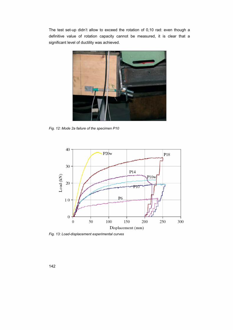
142
The test set-up didn’t allow to exceed the rotation of 0,10 rad: even though a definitive value of rotation capacity cannot be measured, it is clear that a significant level of ductility was achieved.
Fig. 12: Mode 2a failure of the specimen P10
Fig. 13: Load-displacement experimental curves

143
Fig. 14: Moment versus rotation for the specimen P10: a) left joint experimental data b) right joint experimental data c) theoretical model
Capacity design
The capacity design for timber structures can be illustrated through the chain model described in (Paulay & Priestley, 1992) and in Fig.15. As the strength of a chain is the strength of its weakest link, one ductile link may be used to achieve ductility for the entire chain. According to the previously mentioned Eurocode 8 provisions (CEN, 2004), in timber structures the ductile link must be only concentrated in joint (e.g. dowel type joint) whereas the timber elements must be regarded as behaving elastically.
Fig. 15: The capacity design for heavy timber structures according to the chain model.

144
Therefore a reliable strength prediction of the joint and its components is essential for applying the capacity design and ensuring the required ductility. Potentially brittle mechanisms, such as by shear failure or bending failure outside the joint zone, have in fact to be prevented by checking that their actual strength exceeds the strength demand. To this aim, an over-strength coefficient can be adopted in the design of the timber element:
Rd,jovRd,GL M·M γ≥ (32)
where MGL,Rd is the bending strength of the glulam element; Mj,Rd is the bending strength of the joint and γov is a suitable overstrength factor. In the present paper an “engineered” joint is proposed, where the strength prediction methods usually adopted for steel structures can be applied. The experimental campaign showed that the component method provides a reliable prediction of the failures modes, ensuring the possibility to apply the capacity design for the joints. In order to enable activation of a global ductile behaviour of the joint, failure modes involving the plastic deformation of the flange were preferred (mode 1 and 2 of the T-stub in tension), whereas the failure mode associated to the yielding of the glued bars proved to be inadequate to provide a sufficient plastic rotation of the joints (see P20w specimen result in Fig. 13).
Fig. 16: Capacity design for timber structures. RGL stands for reinforced glulam beam, GL stands for glulam beam.

145
In Fig. 16 the theoretical and experimental results for the analyzed joints are compared with the theoretical bending strength of a reinforced glulam beam (RGL), and of a standard glulam beam (GL). It can be noted that if an appropriated steel end-plate thickness is adopted, an over strength factor in Eq. (32) can be ensured. In fact, in all the tests performed the failure modes involved the joint and not in the timber elements. In the cases considered the over-strength of the timber element was guaranteed by the use of steel reinforced glulam beams. The theoretical prediction of RGL bending strength was carried out as for a reinforced concrete section, with a homogenizing parameter obtained as the ratio between the elastic moduli of the different materials.
Conclusions and future works
Owing to the difficulty to obtain energy dissipation in timber elements, the research here presented was addressed to the mechanical characterisation of new joining techniques between timber elements, endowed with local ductility. The results of experimental analysis seem to confirm the high potential of such joints in terms of post-elastic monotonic behaviour and capacity design. Furthermore, the joint model, based on the component method, provides a satisfactory approximation of the test results, in particular for the ultimate load capacity, and failures modes. This represents a first promising step towards the design and analysis of whole framed structures, where steel-to-timber joints are located at the critical sections (Fig. 17).
Fig. 17: Different joint configurations in timber framework structures and portals

146
The current research work is focussed on the deepening the theoretical and experimental knowledge of the joint, which is necessary for the seismic characterisation of the proposed technology. Therefore, a series of cyclic tests on the joints will be the next step of the research. They are designed to provide information of great importance both for an application of the technology in seismic design and for evaluating the global behaviour of a structure with these types of joints. Finally, a simplified model to calculate the rotation at failure of the joint should be set up and validated.
Acknowledgments
The authors gratefully acknowledge the Italian ReLUIS Consortium for partly financing the study, within the research program carried out for the Italian Agency for Emergency Management.
References
[1] Tomasi R., Ductility and pseudo-ductility in timber elements: state of the art, research and development of innovative technologies (in Italian), PhD thesis submitted and awarded 2004, University of Trento
[2] CEN, European Committee for Standardization, EN 1998-1, Eurocode 8: Design of structures for earthquake resistance- Part 1: General rules, seismic actions and rules for building, 2004
[3] Johansen, K. W., Theory of timber connections, IABSE, Publication no. 9, 249-262, 1949
[4] CEN, European Committee for Standardization, EN 1995-1-1, Eurocode 5: Design of timber structures. Part 1-1: General - Common rules and rules for buildings, 2004
[5] DIN Deutsches Institut für Normung e.V., DIN 1052:2004, Design of timber structures. General rules and rules for buildings (in German), 2004
[6] Larsen, H.J., Jensen J.L., Influence of semi-rigidity of joints on the behaviour of timber structures, Progress in Structural Engineering and Materials, vol. 2, 267-277, 2000
[7] Blass H.J., Schmidt M., Self-tapping screws as reinforcement perpendicular to the grain in timber connections, RILEM Symposium on Joints in Timber Structures, Stuttgart (Germany), 163-172, 2001

147
[8] Buchanan A. H., Deng X. J., Strength of Epoxied Steel Rods in Glulam Timber, International World Engineering Conference I.W.E.C., New Orleans (Louisiana, USA), vol. 4, 488-495, 1996
[9] Ranta-Maunus A., Kangas J., Glued-in steel Rods in V-shape, Pacific Timber Engineering Conference PTEC 94, Gold Coast (Australia), vol. 2, 778-784, 1994
[10] Del Senno M., Piazza M., Tomasi R., Axial glued-in steel timber joints – experimental and numerical analysis, Holz als Roh- und Werkstoff, vol. 62, 137-146, 2004
[11] Jaspart J.P., General report: session on connections, Journal of Constructional Steel Research, vol. 55, 69-89, 2000
[12] CEN European Committee for Standardization, EN 1993-1-8. Eurocode 3: Design of steel structures - Part 1-8: Design of joints, 2005
[13] ECCS - European Convention for Constructional Steelwork, member TC 10 Structural Connections, convenor ad-hoc group for Column Base Design (ECCS TC10-COST C1) Document.: Column Bases in Steel Building Frames, Weynand K, BrusselsBruss (eds).Brussels, BE, 1999.
[14] Volkersen O., Die Nierkreaftverteilung in zugbeanspruchten Nietverbindungen mit kostantes Laschenquerschmitten (in German), Luftfahrtvorschung, Band 15, 41-47, 1938
[15] Richart, F., E., Hall, J., R., Woods, R., D., Vibrations of Soils and Foundations, Prentice-Hall, Inc., Engelwood Cliffs, New Jersey, 1970
[16] Bodig J., Jayne B. A., Mechanics of wood and wood composites, New York, Van Nostrand Reinhold, 1982
[17] Gehri E., Ductile behaviour and group effect of glued-in steel rods, RILEM Symposium on Joints in Timber Structures, Stuttgart (Germany), 333-342, 2001
[18] Paulay T., Priestley M.J.N., Seismic design of reinforced concrete and masonry buildings, John Wiley and Sons, 1992

148

149
APPENDICE C
Andreolli M., Piazza M., Tomasi R., Zandonini R., “Ductile moment resistant steel to timber connections”, SPECIAL ISSUE IN TIMBER ENGINEERING, Proceedings of the Institution of Civil Engineers, Structures and Buildings, in press (2011)

150
151
Ductile moment resistant steel-to-timber connections with glued-in rods
Abstract
The research presented investigates the mechanical characterisation of a joint, suitable for different configurations within a heavy timber frame, consisting of a wooden element connected to a steel stub by means of an end-plate and glued-in steel rods. This connection system has some interesting properties in terms of mechanical performance, versatility and high level of prefabrication. An analytical model to predict the joint response in terms of its key parameters (e.g. failure mode, ultimate resistance, stiffness and rotation capacity) is proposed and validated through an extensive experimental campaign. The component method, originally proposed for semi-rigid joints in steel frameworks, is adapted in order to set up a feasible general model for steel to timber joints, enabling application of the capacity design approach and offering the required ductility for applications in seismic zones. The tests carried out indicate satisfactory agreement between theoretical and experimental results: the reliable prediction of joint failure modes allows design of moment resistant connections that can sustain high plastic deformation without brittle rupture, with a remarkable degree of global ductility and energy dissipation under alternate loading.
Notations
As effective bar area B tension in the steel bars Bt,Rd tension resistance of the steel bars beff,c effective width of the flange of the equivalent T-stub in compression di geometrical parameter defined in Fig. 10 Ed energy dissipated in a full cycle Ep available potential energy Es elastic modulus of steel E0,w elastic modulus of wood parallel to the grain F force of the component of the joint Fc,T-stub,Rd resistance of the equivalent T-stub in compression

152
FRd resistance of the weakest component of the joint Fsf,Rd resistance of the steel section flange in compression Ft,bar,Rd resistance of the glued-in steel bars in tension Ft,T-stub,Rd resistance of the equivalent T-stub in tension fu steel ultimate strength fy steel yield strength h depth of the steel section kb stiffness coefficient for the steel bars in tension ki stiffness coefficient kp stiffness coefficient for the steel end-plate in bending under tension kt stiffness coefficient for timber in compression Lb steel bar elongation length leff,c effective length of the flange of the equivalent T-stub in compression leff,t effective length of the flange of the equivalent T-stub in tension M bending moment of the joint m geometrical parameter Mc,Rd moment resistance of the steel section
Mj,Rd moment resistance of the joint n geometrical parameter Q prying force Sj,ini initial rotational stiffness of the joint t time tf end-plate thickness tsf steel section flange thickness V displacement Vy yield displacement x extension of the compression zone z lever arm of the internal couple α numerical coefficient in the definition of the steel bar elongation length β numerical coefficient in equation (8) δb ultimate displacement of the steel bars ∆M/M impairment of bending strength δu,t,T-stub,i ultimate displacement of the T-stub in tension εu ultimate strain of the steel end-plate εub ultimate strain of the steel bars νeq equivalent viscous damping ratio

153
Φ diameter ϕ rotation of the joint ϕCd rotation capacity of the joint
Subscripts
1, 2, 3 failure modes of the equivalent T-stub in tension c compression t tension
Keywords
Timber structures, Seismic engineering, Buildings, Structures & Design
1. Introduction
Structural ductility, which is the capability to withstand large plastic deformations without brittle failure, is a crucial feature for the design of structures in seismic areas, allowing the dissipation of energy by means of ductile hysteretic behaviour. Wood is considered to be, in structural size, a brittle material, with very low post-elastic deformation capacity: timber elements, because of the presence of defects (e.g. knots) and the lack of homogeneity, unlike suitably designed reinforced concrete or steel elements, show brittle behaviour in bending. This remains a problem, even if some recent research investigated the possibility of improving the post-elastic behaviour of glulam beams (Tomasi et al., 2009). As a consequence, in timber structures, energy dissipation is concentrated in the joints, which can resist earthquake action beyond their elastic range, whereas the timber elements are regarded as behaving elastically (EN 1998-1, 2004). In accordance with the capacity design method (Paulay and Priestley, 1992), joints should hence be properly detailed to ensure the required global ductility of the structure. To this aim, joints must possess an appropriate capacity to dissipate energy under severe deformation with limited loss of strength under cyclic loading. Potentially brittle mechanisms, such as shear or bending failure outside the connection zone, must be prevented by checking that the timber elements have sufficient strength. In dowel-type fasteners (e.g. nails, screws, dowels and bolts), where strength is evaluated through expressions based on the European Yield Mode (Johansen, 1949, EN 1995-1-1, 2004), ductility is achieved by means of the plastic deformation in metallic connectors. Light timber frame structures, with a large

154
amount of steel connectors designed to favour steel yielding as the governing mechanism, have proven to present good performance in terms of energy dissipation under seismic action. Moreover the European seismic code gives some detailing rules and provisions for dowel type connectors to determine the maximum fastener diameter, depending on the thickness of the connected timber members, for which ductile mechanisms are favoured. On the contrary in heavy portal frames, the potential for energy dissipation is limited by the low number of joints. The structural form adopted for many types of timber buildings (e.g. industrial and sport buildings) employs portal frames having moment resistant knee connections, generally made using dowel fasteners. A possible option for heavy portal frames is also the use of glued-in steel bars connections for moment resistant corner joints (Buchanan and Fairweather, 1992) and for column to foundation joints (Buchanan and Fletcher, 1989, Kangas et al., 2001). These solutions involve some interesting properties in terms of mechanical performance and aesthetic appearance (since the steel bars are embedded in the timber elements). The development of prefabricated connection systems also favours the reduction of structure erection time and limits work at the construction site. Taking into account this good performance, several authors investigated theoretically and experimentally the mechanical response of the single glued-in bar, inserted both parallel and perpendicular to the grain (Riberholt, 1988, Buchanan and Deng, 1996, Blaß and Laskewitz, 2001, Del Senno et al., 2004). Within the frame of the European Community financed GIROD research program, there has been an international effort to develop this knowledge (Bengtsson and Johansson, 2001). The outcomes of these studies are some proposed expressions to estimate the pull-out resistance. On the code side, no recommendations for the design of glued-in steel bars are provided by European standards, while detailed rules are reported in DIN 1052 (DIN, 2008). Aspects such as the ductility of joints with glued-in rods were investigated by some authors (Gehri, 2001, Gattesco and Gubana, 2006) who studied the failure mechanisms of axially glued-in rods and the possibility of plastic bar deformation before failure, so that ductile behaviour of the joints is ensured. It is worth noting that the ductile behaviour of an axially loaded bar can be associated with the steel yielding and is much affected by the steel grade. Even yield strength higher than nominal can trigger a brittle failure mode, governed by bond and timber failure.

155
In this paper we present a joint for different configurations within a frame, where a timber element is connected to a steel stub by means of an end-plate and glued-in steel rods (Tomasi et al., 2008). An analytical model to predict the joint response in terms of its key parameters (e.g. failure mode, ultimate resistance, stiffness and rotation capacity) is proposed and validated through an extensive experimental campaign. Attention is also focused on the cyclic behaviour of the joint, for the importance of this in seismic design. In particular the strength loss and the energy dissipation under alternate loading of the joint are determined. The joint is conceived and designed to allow plastic flexural deformation of a steel end-plate and to preserve the elastic brittle failure mode of the bar, in order to obtain a connection able to sustain high plastic deformation without brittle rupture.
2. End-plate joint in steel-timber structures
The moment connection theoretically and experimentally studied in this paper is presented in Fig. 1: a stub of steel section (1) is connected to a glued laminated timber element (2) by means of: an end-plate welded on the steel profile (3); steel bars glued-in parallel to the grain (4); a glued-in steel plate inserted in a slot cut in the timber element (5).
Fig. 1. The end-plate steel to timber joint: without (a) or with (b) a glued-in steel plate inserted in a slot grooved in the timber element
The configuration of the joint assures transmission of the bending moment (through end-plate and steel bars) and of the shear force (through the glued-in steel plate) between the timber element and the steel section. When shear forces are low, the joint can be manufactured without the glued-in steel plate: in this case the transmission of lateral loads can be directly supported by the steel bars.
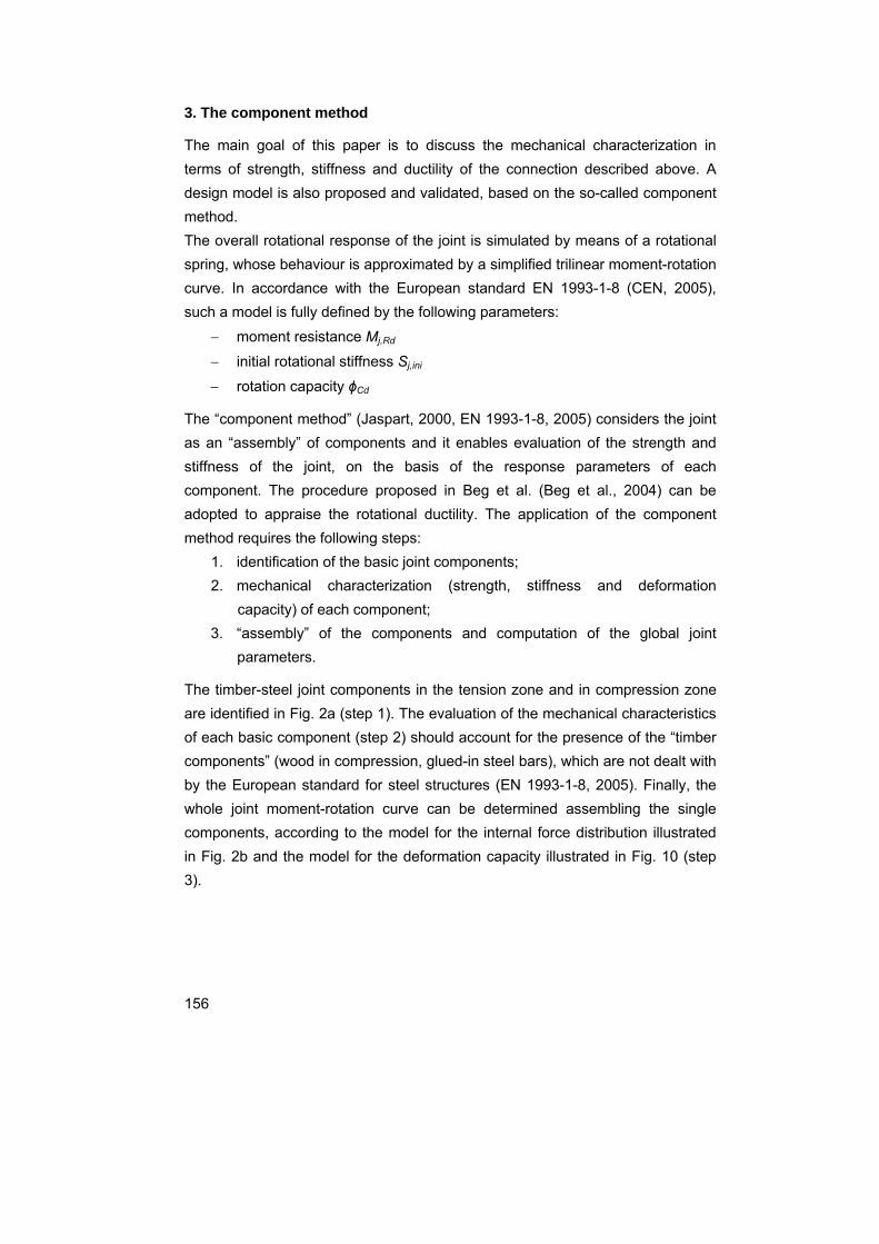
156
3. The component method
The main goal of this paper is to discuss the mechanical characterization in terms of strength, stiffness and ductility of the connection described above. A design model is also proposed and validated, based on the so-called component method. The overall rotational response of the joint is simulated by means of a rotational spring, whose behaviour is approximated by a simplified trilinear moment-rotation curve. In accordance with the European standard EN 1993-1-8 (CEN, 2005), such a model is fully defined by the following parameters:
− moment resistance Mj,Rd
− initial rotational stiffness Sj,ini
− rotation capacity ϕCd
The “component method” (Jaspart, 2000, EN 1993-1-8, 2005) considers the joint as an “assembly” of components and it enables evaluation of the strength and stiffness of the joint, on the basis of the response parameters of each component. The procedure proposed in Beg et al. (Beg et al., 2004) can be adopted to appraise the rotational ductility. The application of the component method requires the following steps:
1. identification of the basic joint components; 2. mechanical characterization (strength, stiffness and deformation
capacity) of each component; 3. “assembly” of the components and computation of the global joint
parameters.
The timber-steel joint components in the tension zone and in compression zone are identified in Fig. 2a (step 1). The evaluation of the mechanical characteristics of each basic component (step 2) should account for the presence of the “timber components” (wood in compression, glued-in steel bars), which are not dealt with by the European standard for steel structures (EN 1993-1-8, 2005). Finally, the whole joint moment-rotation curve can be determined assembling the single components, according to the model for the internal force distribution illustrated in Fig. 2b and the model for the deformation capacity illustrated in Fig. 10 (step 3).

157
Fig. 2. (a) Basic joint components for the steel to timber joint analyzed; (b) model for the internal force distribution and related stiffness
3.1 Joint moment resistance
The design moment resistance can be determined according to:
· z = FM Rdj,Rd (1)
where z is the lever arm of the internal couple (see Fig. 3) and FRd is the resistance of the weakest component of the joint, that is the smallest value among:
− the resistance of the equivalent T-stub in tension Ft,T-stub,Rd
− the resistance of the equivalent T-stub in compression Fc,T-stub,Rd
− the resistance of the steel section flange in compression Fsf,Rd
− the resistance of the glued-in steel bars in tension Ft,bar,Rd

158
Fig. 3. Modelling an extended end-plate as an equivalent T-stub in compression (a) and in tension (b) according to EN 1993-1-8
• An equivalent T-stub in tension, defined according to EN 1993-1-8 (CEN, 2005), is adopted to model the design resistance and failure mode of the extended end-plate in bending, together with the steel bars in tension (see Fig. 3). In Fig. 4 the possible failure modes are shown: complete yielding of the flange (mode 1); failure of the bars after yielding of the flange in presence of prying forces (mode 2) and bar failure (mode 3). The T-stub strength is calculated using Eurocode 3 formulae, where the nominal yield stress fy is replaced by the ultimate strength fu measured by tensile tests on specimens from the same steel plate utilized for the experimental campaign (see Table 1): this is done to consider strain hardening, which mobilizes a significant part of the ultimate resistance. This assumption is important also in association with the prediction of the failure mode: correct identification of the failure mode is essential for assessment of the ultimate rotation of the joint.
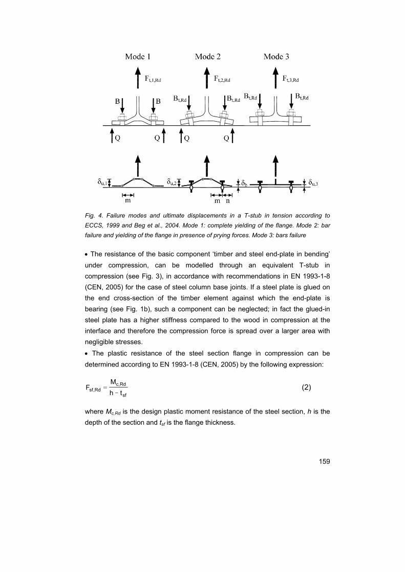
159
Fig. 4. Failure modes and ultimate displacements in a T-stub in tension according to ECCS, 1999 and Beg et al., 2004. Mode 1: complete yielding of the flange. Mode 2: bar failure and yielding of the flange in presence of prying forces. Mode 3: bars failure
• The resistance of the basic component ‘timber and steel end-plate in bending’ under compression, can be modelled through an equivalent T-stub in compression (see Fig. 3), in accordance with recommendations in EN 1993-1-8 (CEN, 2005) for the case of steel column base joints. If a steel plate is glued on the end cross-section of the timber element against which the end-plate is bearing (see Fig. 1b), such a component can be neglected; in fact the glued-in steel plate has a higher stiffness compared to the wood in compression at the interface and therefore the compression force is spread over a larger area with negligible stresses.
• The plastic resistance of the steel section flange in compression can be determined according to EN 1993-1-8 (CEN, 2005) by the following expression:
sf_
Rd,cRd,sf th
MF = (2)
where Mc,Rd is the design plastic moment resistance of the steel section, h is the depth of the section and tsf is the flange thickness.

160
• The yielding of the glued-in steel bars in tension is incorporated in the strength of the equivalent T-stub. Occurrence of the following brittle failure modes should be prevented in the framework of capacity design:
− failure of the adhesive by debonding from steel or wood;
− failure of the timber adjacent to the glue-line;
− failure of the timber member (e.g. pull-out of a whole timber plug with several glued-in rods).
Verification can be made according to the recommendations in DIN 1052 (DIN, 2008); an appropriate overstrength coefficient equal to 1.5, as suggested by CNR DT-206 (CNR, 2007), should be adopted in order to avoid the aforementioned brittle failure modes. In the joints where the shear force is transferred by the steel bars in the compression zone, the shear load-carrying capacity should be determined via the expressions based on the European Yield Model (Johansen, 1949) and adopted in modern standards, assuming a wood embedment strength equal to the 10% of the embedding strength value in the direction perpendicular to the grain (DIN, 2008). The lever arm z (see Fig. 3) should be taken as the distance from the bars in tension to the centre of the stress block of the compression forces: in the case of joints without a bearing steel plate glued on the end cross-section of the timber element, the extension of the compression zone, indicated as x in Fig. 3, can be determined from the translational equilibrium assuming plastic behaviour for wood in compression parallel to the grain (Tomasi et al., 2008).
3.2 Joint rotational stiffness
The initial rotational stiffness Sj,ini should be determined according to EN 1993-1-8 (CEN, 2005) by the following expression:
∑1=2
i
sini,j
k
· zES (3)
where Es is the elastic modulus of steel and ki is the stiffness coefficient for ith basic component in Fig. 2b:
− kp is the stiffness coefficient for the steel end-plate in bending under tension;
− kb is the stiffness coefficient for the steel bars in tension;

161
− kt is the stiffness coefficient for timber in compression.
The other basic components give negligible contribution to the rotational stiffness of the joint.
• The stiffness coefficient kp (steel end-plate in bending under tension) can be determined according to the relationships provided in EN 1993-1-8 (CEN, 2005):
− with prying forces:
3
3850=
m · t · l,
k ft,effp (4)
− without prying forces:
3
34250=
m · t · l,
k ft,effp (5)
where leff,t, tf and m are respectively the effective length, the thickness and a geometrical parameter of the equivalent T-stub flange in tension (Fig. 3).
• The stiffness coefficient kb (two steel bars in tension in a row) can be determined according to the relationships provided in EN 1993-1-8 (CEN, 2005):
− with prying forces:
b
sb L
· A,k
61= (6)
− without prying forces:
b
sb L
· A,k
02= (7)
where As is the effective bar area and Lb is the steel bar elongation length, taken as equal to the sum of α times the nominal bar diameter, the plates thickness, the washer and half of the height of the nut. The dimensionless parameter α, ranging from 1 to 1.5, can be determined taking into account the Volkersen analysis (Volkersen, 1938) for the case of an axial-symmetric joint with a glued-in rod (Tomasi et al., 2008).
• The stiffness coefficient kt for timber in compression is defined as:
s
c,effc,effw,t · E
· lb · Ek
β=
0 (8)
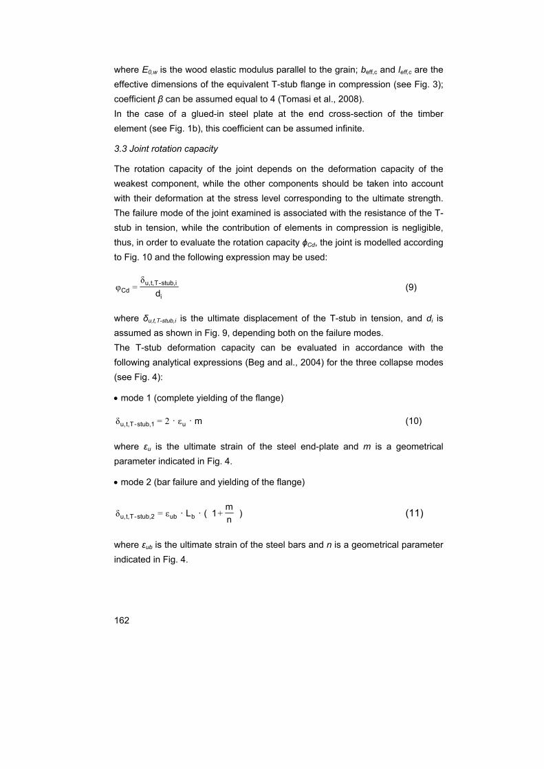
162
where E0,w is the wood elastic modulus parallel to the grain; beff,c and leff,c are the effective dimensions of the equivalent T-stub flange in compression (see Fig. 3); coefficient β can be assumed equal to 4 (Tomasi et al., 2008). In the case of a glued-in steel plate at the end cross-section of the timber element (see Fig. 1b), this coefficient can be assumed infinite.
3.3 Joint rotation capacity
The rotation capacity of the joint depends on the deformation capacity of the weakest component, while the other components should be taken into account with their deformation at the stress level corresponding to the ultimate strength. The failure mode of the joint examined is associated with the resistance of the T-stub in tension, while the contribution of elements in compression is negligible, thus, in order to evaluate the rotation capacity ϕCd, the joint is modelled according to Fig. 10 and the following expression may be used:
d
i
istub,-Tt,u,Cd
δ=φ (9)
where δu,t,T-stub,i is the ultimate displacement of the T-stub in tension, and di is assumed as shown in Fig. 9, depending both on the failure modes. The T-stub deformation capacity can be evaluated in accordance with the following analytical expressions (Beg and al., 2004) for the three collapse modes (see Fig. 4):
• mode 1 (complete yielding of the flange)
· m · ustub,1-Tt,u, ε2=δ (10)
where εu is the ultimate strain of the steel end-plate and m is a geometrical parameter indicated in Fig. 4.
• mode 2 (bar failure and yielding of the flange)
)nm
1( · · L bubstub,2-Tt,u, +ε=δ (11)
where εub is the ultimate strain of the steel bars and n is a geometrical parameter indicated in Fig. 4.

163
• mode 3 (bars failure)
The deformation capacity is simply the elongation of the steel bars at failure:
bubstub,3-Tt,u, · L ε=δ (12)
4. Experimental analysis
4.1 Specimen geometry and materials
Eight specimens, with the same geometry for timber section (120×240 mm) and for steel element (HEB 120), were prepared for monotonic tests. In order to investigate the behaviour of the connection, with special regard to the joint ductility and to the influence of the different failure modes on the capacity in terms of ultimate rotation, the thickness tf of the end-plate (steel grade S235) was varied from 6 to 20 mm (tf = 6 mm; 8 mm; 10 mm; 15 mm; 20 mm). Further details of the steel element geometry are reported in Fig. 5. Both ends of the steel section are welded to a steel plate (full penetration butt weld): the right end-plate is connected to a glued laminated timber beam (strength class GL 24h) by means of 4 steel bars (16 mm of diameter, strength class 6.8); the left end-plate is stiffened and rigidly connected to a reaction base with 4 or 6 bars depending on the specimens.
Fig. 5. Geometry of the end-plate of the steel to timber connection: specimen manufactured with (a) or without (b) the glued-in steel plate (units: mm)
In the specimens manufactured with glued-in steel plates, four holes 18 mm diameter are drilled in the end-plate, in order to allow full transfer of the shear load to the glued-in plate. In the specimens built without the glued-in steel plate, where the shear load is transferred directly by the steel bars, four slotted holes

164
are drilled on the end-plate as shown in Fig. 5b: with this arrangement, the shear load transfer mechanism generates only compression stresses perpendicular to the grain in the timber element, while tension stresses, which can trigger very brittle and low resistance collapse modes, are prevented. The list of the specimens tested monotonically is reported in Tab. 1: the specimens manufactured with the glued-in steel plate for the shear load are indicated as “Px-sp”, x being the end-plate thickness in mm, (P6-sp; P8-sp; P10-sp; P15-sp; P20-sp), whilst those where the shear force is transferred by the steel bars are indicated as “Px” (P6; P8; P10). Eight further specimens with the same geometry as for monotonic tests were tested under cyclic loading.
Specimen End-plate steel Failure mode of T-
stub in tension Moment resistance
(kNm) Rotation capacity (rad)
εu %
fy (MPa)
fu (MPa) Th. Exp. Theoretical Experimental
* Theoretical Experimental **
P6-sp 38,5 299,6 377,2
1 1 7,08 15,07 0,15 0,20
P6 1 1 6,56 8,85 0,15 0,15
P8-sp 38,6 275,5 367,5
1 2 10,66 16,59 0,16 0,19
P8 1 2 10,51 14,99 0,16 0,21
P10-sp 45,9 256,1 374,0
2 2 15,37 17,14 0,14 0,12
P10 2 2 15,80 19,85 0,13 0,18
P15-sp 35,7 295,5 383,1 2 2 21,82 24,54 0,13 0,14
P20-sp 36,4 278,2 400,6 3 3 28,51 32,29 0,06 0,07
* maximum value ** displacement at failure Tab.1: Comparison between theoretical model and experimental results in terms of: failure modes for T-stub in tension (see fig. 4), strength values and rotation capacity of the joint
The manufacturing process is illustrated in Fig. 6. On the end cross-section of the timber element (see Fig. 6a) four holes diameter 20 mm are drilled, with length ranging from 50 cm to 100 cm, in order to allow adequate anchorage of the bars. A two component epoxy resin is poured into the holes and threaded steel bars are inserted. To ensure that the steel bars are placed concentrically in the drilled holes, a template is used and removed after adhesive curing. A similar procedure is adopted to insert the glued-in steel plate: grooving of a central slot at the end cross-section of the timber element; pouring the glue, introduction of the perforated web of the steel T-shape as in Fig. 6b.

165
Fig. 6. Manufacturing process: (a) gluing the threaded steel bars into machine drilled holes (specimen without a glued-in steel plate for shear forces); (b) insertion of the glued-in steel plate for shear forces (note the ends of the bars are protected in order to avoid spreading the glued on the thread)
4.2 Test set-up and protocol
The test set-up was designed so that bending and shear are both acting on the joint (see Fig. 7) and was used for both the monotonic and the cyclic tests. A cantilever configuration was adopted, where the steel stub element is rigidly connected at one end to the reaction floor of the laboratory; the load was applied by a hydraulic jack at a distance of 2000 mm from the joint under investigation. The end-plate connecting the steel stub and the reaction floor was adequately stiffened as illustrated in Fig. 5 in order to ensure failure at the steel to timber joint. The connection between the hydraulic jack and the timber beam was designed to act as a ‘perfect’ hinge.

166
Fig. 7. Set-up for monotonic and cyclic tests: (1) steel profile connected to the reaction base; (2) displacement transducer 100 mm; (3) displacement transducer 500 mm; (4) load cell; (5) hydraulic jack; (6) cyclic test protocol according to EN 12512
The instrumentation layout is illustrated in Fig. 7: the applied force was measured by a load cell (4); the rotation of the joint was detected by two displacement transducers (2) measuring the relative displacement between the steel profile and the timber beam, while two displacement transducers (3) were placed along the timber beam (at the hydraulic jack and at the mid-length of the cantilever). In monotonic tests the loading was applied under displacement control at a constant rate of 0,2 mm/sec so that failure was achieved in about 30 minutes. The loading history in cyclic tests is shown in Fig. 7: in accordance with the procedure described in the European standard EN 12512 (CEN, 2005) for timber joints, the amplitude of the cycles is defined as a function of the yield displacement Vy, determined experimentally in the corresponding monotonic test. The rate of displacement increase was constant within each cycle, but varied from 0,2 mm/s to 1 mm/s during the entire process (which lasted approximately 2 hours). Other details of the set-up and connection system are reported in Fig. 8 and in Fig. 9.

167
Fig. 8. Set-up for monotonic test: failure displacement of the specimen P6-sp
Fig. 9. Detail of connection system at failure displacement of specimen P8
4.3 Results of the monotonic tests
In Tab. 1 the types of failure modes observed, the moment resistance and the rotation capacity are reported for all the joints tested monotonically, and compared with the theoretical results. Moreover, for three specimens chosen as representative of the three theoretical failure modes (P6, P10 and P20-sp), Fig. 10 illustrates the condition at failure, while Fig. 11 provides the experimental and theoretical moment-rotation relationship.

168
Fig. 10. Failure modes and associated deformation capability δu,i, as observed in the experimental campaign: (a) mode 1 in specimen P6 with complete yielding of the flange; (b) mode 2 in specimen P10 with bar failure and flange yielding in the presence of prying forces; (c) mode 3 in specimen P20-sp with bar failure
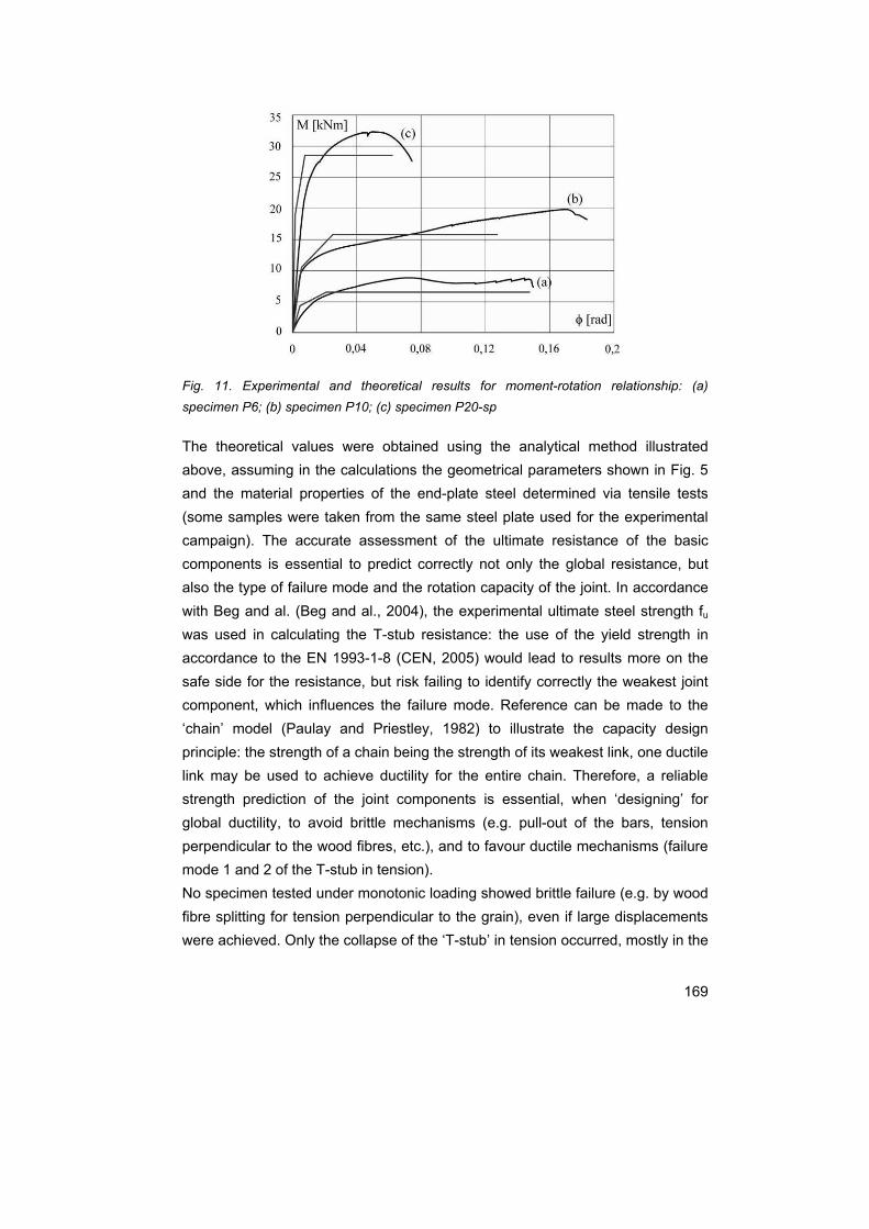
169
Fig. 11. Experimental and theoretical results for moment-rotation relationship: (a) specimen P6; (b) specimen P10; (c) specimen P20-sp
The theoretical values were obtained using the analytical method illustrated above, assuming in the calculations the geometrical parameters shown in Fig. 5 and the material properties of the end-plate steel determined via tensile tests (some samples were taken from the same steel plate used for the experimental campaign). The accurate assessment of the ultimate resistance of the basic components is essential to predict correctly not only the global resistance, but also the type of failure mode and the rotation capacity of the joint. In accordance with Beg and al. (Beg and al., 2004), the experimental ultimate steel strength fu was used in calculating the T-stub resistance: the use of the yield strength in accordance to the EN 1993-1-8 (CEN, 2005) would lead to results more on the safe side for the resistance, but risk failing to identify correctly the weakest joint component, which influences the failure mode. Reference can be made to the ‘chain’ model (Paulay and Priestley, 1982) to illustrate the capacity design principle: the strength of a chain being the strength of its weakest link, one ductile link may be used to achieve ductility for the entire chain. Therefore, a reliable strength prediction of the joint components is essential, when ‘designing’ for global ductility, to avoid brittle mechanisms (e.g. pull-out of the bars, tension perpendicular to the wood fibres, etc.), and to favour ductile mechanisms (failure mode 1 and 2 of the T-stub in tension). No specimen tested under monotonic loading showed brittle failure (e.g. by wood fibre splitting for tension perpendicular to the grain), even if large displacements were achieved. Only the collapse of the ‘T-stub’ in tension occurred, mostly in the

170
more ductile modes 1 and 2, but for the specimen P 20-sp with the higher thickness of the steel end-plate, which collapsed according to mode 3. Table 1 shows that the analytical model can predict the experimental failure mode for almost all of the specimens, except P8-sp and P8, which failed in mode 2, while mode 1 was predicted. The ultimate rotation capacity of the joint can also be evaluated satisfactorily by means of the model described above, whose accuracy is strongly correlated to correct identification of the failure mode. As to this point, it is interesting to note that the ‘actual’ failure mode for the specimens P10-sp and P10 can be predicted only by assuming the ultimate strength for the end-plate steel. The use of the yield stress would lead to a more conservative assessment of the resistance; however, it would associate the failure with the wrong mode and, as a consequence, the ultimate rotation capacity of the joint might not be on the safe side. For the specimens manufactured without glued-in steel plate, and where the shear load is transferred through the glued-in steel bars, it can be observed that no specimen showed a failure mode associated with the stresses orthogonal to the fibres at the interface with steel bars; the wood is able to bear the steel end-plate deformation and to make prying forces arise, leading to the same failure modes observed in the corresponding specimen with the steel plate, and also to similar values in terms of moment resistance and rotation capacity (see Fig. 12).
Fig. 12. Monotonic failure mode 2 observed in specimen P10 (without a glued-in steel plate): wood can produce prying forces in the end-plate

171
4.4 Results of the cyclic tests
Cyclic tests were carried out in accordance with the standard EN 12512 (CEN, 2005), which prescribes a loading history comprising of series of cycles at increasing amplitude, defined as a multiple of the yielding displacement Vy previously determined through the monotonic procedure (see Fig. 7). All specimens tested under cyclic load collapsed for failure in bending of the end-plate near the weld due to low cyclic fatigue (see Fig. 13), except for P20-sp specimen, where a local bar failure mechanism was observed. Fracture of the end-plate occurred after a number of cycles at large plastic displacement, with a limited reduction of resistance in subsequent cycles of the same set. In Fig. 14, for three specimens chosen as representative of the three theoretical failure modes (P6, P10 and P20-sp), the hysteretic moment-rotation relationships are compared to the monotonic experimental curves.
Fig. 13. Cyclic failure mode of P15-sp specimen: collapse of the plastic hinge in the end-plate near the weld due to low cyclic fatigue
Two important parameters for seismic performance are reported in Table 2: an estimate of the energy dissipation by hysteresis through the equivalent viscous damping ratio; the reduction of strength for each subsequent set of cycles. Both these parameters, νeq and ∆M/M, defined according to the standard EN 12512 (CEN, 2005), must be considered when assessing the ductility and dissipation capacity of the joint, and hence of the frame.

172
Fig. 14. Monotonic and cyclic experimental results for moment-rotation relationship: (a) specimen P6; (b) specimen P10; (c) specimen P20-sp

173
Specimen
νeq (%) ∆M/M (%)
0,75Vy Vy 2 Vy 4 Vy 6 Vy 8 Vy 0,75V
y
Vy 2 Vy 4 Vy 6 Vy 8 Vy
P6-sp 4,8 8,9 19,7 27,4 26,9 - 0,1 0,7 1,5 3,6 23,3 - P6 8,4 12,4 20,3 23,9 22,6 - -1,5 0,8 1,5 5,3 22,3 - P8-sp 2,5 6,0 18,3 25,7 27,0 22,7 -0,3 0,6 1,2 3,0 9,2 24,7 P8 7,5 13,1 23,1 27,1 28,0 15,2 -0,8 1,6 1,8 6,1 17,5 36,9 P10-sp 3,9 6,8 20,0 26,1 27,7 23,9 -0,1 0,3 2,5 2,6 8,8 16,8 P10 4,4 9,4 20,5 26,4 28,6 30,2 -1,2 1,1 3,0 7,7 10,5 16,6 P15-sp 0,0 0,1 12,6 26,1 33,0 7,9 0,1 0,1 -1,3 3,6 46,2 38,8 P20-sp 0,2 0,6 7,4 - - - 0,4 0,6 3,1 - - -
Tab. 2: Experimental results for cyclic tests: equivalent viscous damping ratio νeq and bending strength deterioration ∆M/M (%) for each set of three cycles at each tested displacement amplitude (multiple of the joint yield displacement Vy) according to the standard EN 12512
The equivalent viscous damping ratio νeq, computed for every third repeated cycle in the cycling procedure adopted, is defined as:
p
deq · E ·
E
π2=ν (13)
where Ed is the energy dissipated in a full cycle, and Ep is the available potential energy. The reduction of strength ∆M/M is defined as the reduction in the bending moment when attaining a given joint rotation from the first to the third cycle of the same amplitude. It is worth noting that the values of the damping ratio at the yield displacement Vy obtained from the experimental results are for all specimens, save P15-sp and P20-sp, comparable with that recommended in literature for bolted steel structures (Newmark and Hall, 1982). The Eurocode 8 provisions for timber structures (CEN, 2004) state that the dissipative zones, which must be considered concentrated only in joints, shall be able to deform plastically for at least three fully reversed cycles at a static ductility ratio of 4 for structures with a medium capacity to dissipate energy and at a static ductility ratio of 6 for high ductile structures, without more than a 20% reduction of their resistance. All the joints tested, save specimen P20-sp, showed the required plastic deformation capacity, with similar values of energy dissipated (νeq = 24-27% for 4 Vy; νeq = 22-33% for 6 Vy).

174
However, only specimens with an end-plate thickness of 8 and 10 mm, at 6Vy satisfy the limit of 20% of reduction of resistance between the first and the third cycle, and can hence be classified as highly dissipative. The other specimens, save P20-sp, should be classified as possessing a medium dissipation capacity.
5. Conclusions and future works
The research presented addresses the mechanical characterisation of a joint suitable for different configurations within a timber frame, consisting in a wooden element connected to a steel stub by means of an end-plate and glued-in steel rods. This connection system involves some interesting properties in terms of: mechanical performance, since semi-rigid connection can be designed without significant reduction of bending capacity; versatility, since various geometries can be adopted for construction of moment resistant joints (e.g. corner and foundation frame joints, see Fig. 15); high level of prefabrication, since the construction assembly can be done using steel structure methods, reducing the erection time of heavy timber structures and limiting work in situ. Similar joint configurations with glued-in rods have been proposed and studied by other authors. So far, an aspect not sufficiently investigated is the possibility of implementing a seismic design approach for moment resistant joint configurations with glued-in rods. This study stresses the need to have a reliable design model for practitioners and researchers in order to correctly predict the mechanical behaviour of the joint also in terms of capacity design. The above illustrated experimental results validated the approach proposed by the authors, where the component method, originally proposed for steel structures, was adapted for steel to timber joints. Monotonic tests demonstrated a satisfactory agreement between theoretical and experimental results for strength values, failure modes and rotation capacity. The validation of the model represents an important step towards the design and analysis of whole frame structures, when the proposed steel to timber joints are adopted in the critical zones. As a matter of fact, in order to enable activation of a global ductile behaviour of the joint, the capacity design approach can be adopted so that failure modes 1 and 2 of the T-stub in tension (involving plastic deformation of the steel end-plate) are favoured, while failure mode 3 (where the end-plate remains elastic and the glued-in bars yield) is prevented, being proved to be inadequate to provide sufficient plastic rotation of the joints.

175
The results of the cyclic tests confirm the high post-elastic ductility of joints designed to fail by mode 1 or 2 of a T-stub in tension (specimens with an end-plate thickness from 6 to 15 mm). Failure mode 3, observed in specimen P20-sp, leads to fairly brittle responses (see Fig. 14). Nevertheless, some differences in terms of dissipation capacity according to Eurocode 8 were observed, depending on the different levels of strength reduction measured during the cyclic tests. These differences stress the need to perform cyclic tests when the dissipation capacity of structural components or elements has to be reliably determined. Future research efforts will be devoted to numerical investigation of the proposed steel to timber joint in single and multi-storey heavy timber frameworks. Non-linear seismic analysis (e.g. push-over analysis) will also be performed in order to determine the behaviour factor to be adopted in design as a function of the inherent ductility of the joints.
6. Acknowledgment
The authors gratefully acknowledge the Italian ReLUIS Consortium for partly financing the study, within the research program carried out for the Italian Agency for Emergency Management.
Fig. 15. Possible applications of the analyzed joint in timber portal frames for moment-resist ant joints at the corner and moment-resistant joints at the foundations

176
References
[1] Beg D., Zupancic E., Vayas I., On the rotation capacity of moment connections, Journal of Constructional Steel Research, 2004, 60, 601–620.
[2] Bengtsson C., Johansson C.J., GIROD - Glued-in rods for timber structures, Proceedings of the 34th CIB W18 meeting, Venice, Italy, 2001, CIB W18/34-7-8.
[3] Blass H.J., Laskewitz B., Load-carrying capacity of axially loaded rods glued-in perpendicular to the grain, Proceedings PRO 22, International RILEM Symposium on Joints in Timber Structures, RILEM Publications S.A.R.L., Stuttgart, Germany, 2001, 363-371.
[4] Buchanan A. H., Fairweather R. H., Epoxied moment-resisting connections for timber buildings, Proceedings of the International Workshop on Wood Connectors, Las Vegas, Nevada, U.S.A., 1992, 107-113.
[5] Buchanan A.H., Deng X. J., Strength Epoxied Steel Rods in Glulam Timber, Proceedings of the International Wood Engineering Conference '96, New Orleans, U.S.A., 1996, 4, 488-495.
[6] Buchanan A.H., Fletcher M.R., Glulam Portal Frame Swimming Pool Construction, Proceedings of the Second Pacific Timber Engineering Conference, Auckland, New Zealand, 1989, 1, 245-249.
[7] CEN, European Committee for Standardization, Timber structures. Test methods. Cyclic testing of joints made with mechanical fasteners, 2005, EN 12512.
[8] CEN, European Committee for Standardization, Eurocode 3: Design of steel structures - Part 1-8: Design of joints, 2005, EN 1993-1-8.
[9] CEN, European Committee for Standardization, Eurocode 5: Design of timber structures. Part 1-1: General - Common rules and rules for buildings, 2004, EN 1995-1-1.
[10] CEN, European Committee for Standardization, Eurocode 8: Design of structures for earthquake resistance - Part 1: General rules, seismic actions and rules for buildings, 2004, EN 1998-1.
[11] CNR, National Research Council, Instruction for design, execution and control of timber structures (in Italian), 2007, CNR-DT 206/2007.

177
[12] Del Senno M., Piazza M., Tomasi R., Axial glued-in steel timber joints - experimental and numerical analysis, Holz als Roh- und Werkstoff, 2004, 62, 137-146.
[13] DIN Deutsches Institut für Normung, Design of timber structures. General rules and rules for buildings (in German), 2008, DIN 1052.
[14] ECCS European Convention for Constructional Steelwork, member TC 10 Structural Connections, Column Bases in Steel Building Frames, Weynand K., Brussels, BE, 1999, Report ECCS TC10-COST C1.
[15] Gattesco N., Gubana A., Performance of Glued-in Joints of Timber Members, Proceedings of WCTE 2006 - 9th World Conference on Timber Engineering, Portland, U.S.A., 2006.
[16] Gehri E., Ductile behaviour and group effect of glued-in steel rods, Proceedings PRO 22, International RILEM Symposium on Joints in Timber Structures, RILEM Publications S.A.R.L., Stuttgart, Germany, 2001, 333-342.
[17] Jaspart J.P., General report: session on connections, Journal of Constructional Steel Research, 2000, 55, 69-89.
[18] Johansen K.W., Theory of Timber Connections, IABSE - International Association of Bridge and Structural Engineering, Bern, Publication No. 9, 1949, 249–262.
[19] Kangas J., Kevarinmäki A., Lumiaho H., Timber Structures with Connections Based on in V-Form Glued-In Rods, Proceedings of IABSE Conference ‘Innovative Wooden Structures and Bridges’, Lahti, Finland, 2001, 85, 585 – 590.
[20] Newmark N. M., Hall, W.J., Earthquake spectra and design, Earthquake Engineering Research Institute, 1982.
[21] Paulay T., Priestley M.J.N., Seismic design of reinforced concrete and masonry buildings, John Wiley and Sons, 1992.
[22] Riberholt H., Glued Bolts in Glulam - Proposal for CIB Code, Proceedings of the 21th CIB W18 meeting, Parksville, Canada, 1988, CIB W18/21-7-2.
[23] Tomasi R., Piazza M., Parisi M.A., Ductile design of glued-laminated timber beams, Practice Periodical of Structural Design and Costruction ASCE, 14, No. 3, 2009, 113-122.

178
[24] Tomasi R., Zandonini R., Piazza M., Andreolli M., Ductile End Connections for Glulam Beams, Structural Engineering International, IABSE, 18, No. 3, 2008, 290-296.
[25] Volkersen O., Die Nietkraftverteilung in zugbeanspruchten Nietverbindungen mit konstanten Laschenquerschnitten (in German), Luftfahrtvorschung, 15, 1938, 41–47.