Give it, Live it, Doing the Pivot

Louise Cape, James Colombo, Katie McDonald, Tammy Rowland

There are many advantages for creating master data file. Once all district data has been compiled a Pivot Table can be easily accessed to pull:● District proficiency data● School, teacher, course and period

proficiency data● High flyers by course/teachers/periods

Give it: Why use a Pivot Table?

Doing the Pivot:

“A pivot table is a special Excel tool that allows you to summarize and explore data interactively. It's a lot harder to explain a pivot table than to show you how one works, so let's take a look.”Excel video tip: What is a pivot table?

https://exceljet.net/tips/what-is-a-pivot-table (2:45)Source: http://www.google.com/#q=what+is+a+pivot+table

Live it: Pivot Tables for District Use

Once the Data Extracts are complete and compiled into one worksheet, data can be pulled to provide district detailed reports in CTE.

Extracting Data from FILR

https://filr.dpi.state.nc.usNet Folders

CTELEA Number

state assessmentsdownload each file

Saving files in Excel

Multiple files from FILR are compiled into one Excel file by cutting and pasting each download into a master spreadsheet. Let’s save our work. Now we are ready to begin.1. In your spreadsheet, make sure all the student scores

are number format with zero decimal places.a. Highlight the column containing the scale

scores—column Qb. On the home ribbon, number group, choosenumber and zero decimal places

Preparing Master Spreadsheetc. This next step adds a column that links together (concatenate) columns L (course code) andcolumn M (course name) into one column so both will show up in a cleaner format for your pivot table. i. Highlight column N ii. On the home ribbon, click Insert, Insert Sheet Columns iii. In “the new” cell N1, type Course Number and Name iv. In cell N2, type the formula, =CONCATENATE(L2&"-"&M2) and enter to make the spreadsheet accept your formula. This formula joins the course number and course name and puts a hyphen between the two.Fill the formula down. A quick way to fill down is to double left mouse click on the lower right hand corner of cell N2

Preparing Master Spreadsheet2. Insert a column between columns R and S and in the new cell S1 key in Proficiency as the column heading.3. Key in the following formula in cell S2:

a. =IF(R2<=76,"Unmet","Met") then tap the enter key to make the spreadsheet accept theformula.

b. Fill the formula down...BEWARE that empty cells in column R will stop the fill downprocess if you are doing it by double clicking on the bottom right corner of cell S2. You willhave to drag it down. (NOTE: you will have empty cells in column R if your LEA administered field tests. We will omit field test data when we build our pivot table).

Doing the Pivot: Inserting the Pivot Table

Inserting the Pivot Table:4. Highlight the whole excel spreadsheet5. Go to the Insert Tab and Click on the Pivot Table Icon6. Make certain to put the table in a New Worksheet is selected and click

OK7. For our example today, click to include School, Teacher, CourseNumber and Name8. Drag and drop Proficiency to the Values section of the pivot table AND theColumns section of the pivot table. NOTE: If your pivot table field list on the right hand of your screen disappears,

just click in your pivot table and it will reappear.

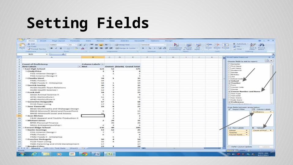
Setting Fields

Delete Blank Columns and Rows9. To delete blank columns and blank rows in your pivot table, click the down arrows by the column labels and row labels and take the checkmark off of blank.

Adding the Proficiency10. To add the proficiency column to your pivot table, click in cell E5 in your pivot table and key in

=b5/d5 and move off the cellor enter to have the program accept your formula. Fill the formula down. 11. Format this column as % with no decimal places.

Proficiency of Zero12. YOU WILL NOTICE THAT FIELD TEST COURSES ARE SHOWING A PROFICIENCY OF ZERO

SINCE THERE IS NO VALUE IN THE SCALE SCORE COLUMN OF OUR SPREADSHEET. Delete them from your pivot table by clicking the down arrow by Course Number and Name andtake the checkmark off of BD10, BF05 and FA32 (Multimedia and Webpage Design, PersonalFinance and Apparel and Textile Production II and blank if showing).

NOTE: Deleting these courses, will cause a few error messages to show up at the bottom ofyour pivot table, you can delete them or just make sure you do not print them. Theylook like this #DIV/0!

Proficiency of Zero

Make your Pivot Attractive13. Now you can edit your pivot table to make it look more attractive. One thing you might like to do is color code the proficiency column. To do this, highlight the percent information under the Proficiency column in your pivot table.14. On the Home Ribbon, Choose Conditional Formatting, Manage Rules

a. New Ruleb. Format Only Cells that Containc. Cell Value, Greater Than or Equal to and type in 77% (don’t forget to type the % sign)d. Formate. Choose your fill color (many people use green), you can make the font bold etc.f. Click OK, OKg. Click New Ruleh. Format Only Cells that Containi. Cell Value, Less than 77% (don’t forget to type the % sign)j. Formatk. Choose your fill color (many people use red), you can make the font bold etc.l. Click OK, OK, Apply, OK

Adding Borders, Titles, and HeadersNow you can continue to add borders, titles, headers, etc. to your pivot table before printing. If you copy your pivot table into another spreadsheet to share with others, anyone can click on the numbers in the grand total section and the student data will display (names, individual scores, etc.). To keep this from happening, depending on your version of Office, you will copy then choose to past values and number formatting or paste special.