global dual sourcing and order smoothing: the impact of

MANAGEMENT SCIENCEVol. 61, No. 9, September 2015, pp. 2080–2099ISSN 0025-1909 (print) � ISSN 1526-5501 (online) http://dx.doi.org/10.1287/mnsc.2014.1992

© 2015 INFORMS

Global Dual Sourcing and Order Smoothing:The Impact of Capacity and Lead Times

Robert N. BouteTechnology and Operations Management, Vlerick Business School, 3000 Leuven, Belgium; and

Research Center for Operations Management, KU Leuven, 3000 Leuven, Belgium, [email protected]

Jan A. Van MieghemKellogg School of Management, Northwestern University, Evanston, Illinois 60208,

[email protected]

After decades of offshoring production across the world, companies are rethinking their global networks.Local sourcing is receiving more attention, but it remains challenging to balance the offshore sourcing cost

advantage against the increased inventories, because of its longer lead time, and against the cost and (volume)flexibility of each source’s capacity. To guide strategic allocation in this global network decision, this paperestablishes reasonably simple prescriptions that capture the key drivers. We adopt a conventional discrete-timeinventory model with a linear control rule that smoothes orders and allows an exact and analytically tractableanalysis of single- and dual-sourcing policies under normal demand. Distinguishing features of our model are thatit captures each source’s lead time, capacity cost, and flexibility to work overtime. We use Lagrange’s inversiontheorem to provide exact and simple square-root bound formulae for the strategic sourcing allocations and thevalue of dual sourcing. The formulae provide structural insight on the impact of financial, operational, anddemand parameters, and a starting point for quantitative decision making. We investigate the robustness of ourresults by comparing the smoothing policy with existing single- and dual-sourcing models in a simulation studythat relaxes model assumptions.

Keywords : inventory; capacity; dual sourcing; production smoothing; mixed-mode transportationHistory : Received November 20, 2012; accepted April 26, 2014, by Yossi Aviv, operations management. Published

online in Articles in Advance October 17, 2014.

1. Introduction and SummaryOver the past few decades it became conventionalwisdom that factory jobs could be done cheaply in somefar-flung corner of the world. The original impetusbehind offshoring for western firms was to reap savingsfrom performing work in overseas countries with lowerwages and materials costs. For several decades thatstrategy worked, often brilliantly, but now companiesare rethinking their global networks. A special reportin The Economist (2013) on offshoring and outsourcingdescribes the story of Lenovo, a Chinese technologygroup, opening a U.S. computer manufacturing linein North Carolina. The global labor “arbitrage” isrunning out: wages in China have nearly doubledsince 2008, partly as a result of domestic minimum-wage policies (the country’s 2011 five-year plan calledfor a 13% average annual minimum-wage increase, arate some provinces already exceeded (George et al.2014)). The cost of shipping goods around the worldhas been rising sharply, and goods spend weeks intransit. Offshoring also often requires substantial safetyinventory, the holding cost of which can outweighthe labor and materials cost advantage. Today, greateremphasis is placed on proximity to demand: responding

to customers’ new-product requests, shorter deliverytimes, and swift corrections to improve designs andquality has magnified the need for responsive andflexible supply chains. Local sourcing therefore isreceiving increasing attention.

A complete reversal to local sourcing, however, maybe unlikely and ill-advised. Indeed, the concepts ofglobal and local sourcing are not mutually exclusive.Rather, the combined use of multiple supply sources,each of which is different and possesses unique advan-tages, might be better than any single-sourcing strategy.Admittedly, multisourcing involves higher coordina-tion costs, but a strategically configured portfolio ofsuppliers with complementary skills can often performbetter than any individual supplier.

In this paper we analyze global sourcing for compa-nies that have access to two sources with complemen-tary competencies: a local source that is responsivebut more expensive, and a global source that is (glob-ally) more cost-efficient but with a longer lead time.1

1 Supply competencies can correspond to transportation modes sothat our analysis also applies to balancing mixed-mode transportationor spot and forward market purchasing.

2080

Dow

nloa

ded

from

info

rms.

org

by [

129.

105.

199.

87]

on 0

6 O

ctob

er 2

015,

at 1

1:41

. Fo

r pe

rson

al u

se o

nly,

all

righ

ts r

eser

ved.

Boute and Van Mieghem: Global Dual Sourcing and Order SmoothingManagement Science 61(9), pp. 2080–2099, © 2015 INFORMS 2081

Although our policy can be used for two local sources,we adopt the setting where the low-cost source isoffshore and far away from the local responsive source.Whereas the sourcing literature typically only considerssourcing and inventory related costs, we explicitly addeach source’s capacity cost and flexibility (modeledby its cost to work overtime). In the current economicclimate of rising labor costs in some countries, anddecreasing flexibility to go beyond regular workinghours (driven by strong labor unions or by capacityrigidity due to high levels of automation), capacitycost and flexibility are increasingly relevant factorsfor sourcing decisions. The Economist (2013) mentionsthat one of the reasons why reshoring may less likelyhappen in Europe, compared to the United States, isbecause Europe’s labor markets are still fairly inflexibleand costly. Labor flexibility still varies greatly fromcountry to country. In a global economy where firmscan go where they want, these differences have aneffect.

Our approach assumes a wholly owned global net-work where capacity costs and flexibility are directlyrelevant. We believe this approach provides a steppingstone to a decentralized system, where independentsuppliers will in one way or another include a sourcingcharge for capacity costs and flexibility, but a formalgame-theoretic analysis is left for future research.

We adopt a conventional discrete-time inventorymodel with stochastic demand and a linear control rulethat is capable of smoothing orders to both sources.The reasons for analyzing this policy, which we willrefer to as dual-sourcing smoothing (DSS), are thatsmoothing policies are effective to reduce capacityrequirements and are used in practice (see empiricalevidence in §2) when companies face high labor orcapital capacity costs. In addition, the linearity ofsmoothing policies provides analytic tractability withnormally distributed demand and allows us to specifyanalytically the strategic sourcing allocations to bothsources.

The optimality equations involve a polynomial ofdegree higher than the lead time difference L betweenthe two sources. Given that a quartic is the polynomialof highest degree for which general finite analyticexpressions for the roots can exist, we use Lagrange’sinversion formula to solve the optimality equations forgeneral L. Another technical contribution, for whichwe relied on Lagrange’s technique, is the inclusionof general lead times for each source in a smoothingpolicy. To the best of our knowledge, the application ofthe Lagrange series to inventory theory appears novel.

The main contribution of this paper is to providemanagerial guidelines for strategic sourcing (global,local, or dual sourcing) based on exact formulae andsimple square-root bounds that capture the impact ofeach source’s cost, lead time, capacity, and flexibility for

normally distributed demand. Specifically, we presenta simple guideline that captures the trade-off betweenthese four parameters when deciding between local orglobal single sourcing with the standard base-stock pol-icy. We show that single sourcing with order smoothingdominates using a base-stock policy in the presenceof capacity costs and performs close to the optimalsourcing policy under capacity costs. We then extendorder smoothing to dual sourcing and present formulaeand bounds that specify the optimal volume fractionordered from the global source (the strategic offshoringallocation), its corresponding total landed cost, and thevalue of dual sourcing (over single sourcing).

We show that order smoothing policies shine whendual sourcing faces capacity costs, inflexibility, or longerlead time difference L between both sources. The maxi-mal value of dual-sourcing smoothing then increasessignificantly and grows at the order of L1/6. Moreover,the parameter region for which dual-sourcing smooth-ing dominates capacitated single sourcing widens as Lincreases. The square-root formulae that we presentare sufficiently simple to provide a starting point forquantitative decision making to optimally trade off costand responsiveness. Although simple, the formulae stillcapture the key parameters and thus provide structuralinsight on the impact of financial, operational, anddemand parameters on dual-sourcing decisions.

Finally, a simulation study demonstrates the robust-ness of our results by relaxing the normality assumptionand by comparing the policy with other policies studiedin the literature.

2. Related LiteratureOur work directly relates to two streams of research:dual-sourcing inventory models and order smoothingpolicies. The dual-sourcing literature refers to inventorymodels where replenishment occurs through a regularchannel and/or a more expensive, but faster expeditedchannel. The objective is to minimize the expectedsum of procurement, holding, and shortage costs overmultiple periods. The dual-sourcing literature is veryrich; we focus primarily on discrete review models.Fukuda (1964) shows that when the lead time differenceis one period, dual-base-stock policies are optimal. In adual-base-stock policy, an expedited order is placedto bring the inventory position up to a first (expedite)base-stock level, after which a regular order is placed tobring it up to a second and higher (regular) base-stocklevel. Fukuda uses first-order conditions to deriveexpressions for the base-stock levels. Whittemore andSaunders (1977) extend Fukuda’s (1964) model andshow that when lead times differ by more than oneperiod, the optimal policy is no longer a dual basestock, but it depends on the entire ordering historyand requires multidimensional dynamic programming.

Dow

nloa

ded

from

info

rms.

org

by [

129.

105.

199.

87]

on 0

6 O

ctob

er 2

015,

at 1

1:41

. Fo

r pe

rson

al u

se o

nly,

all

righ

ts r

eser

ved.

Boute and Van Mieghem: Global Dual Sourcing and Order Smoothing2082 Management Science 61(9), pp. 2080–2099, © 2015 INFORMS

Optimal dual-sourcing policies are, in general, highlycomplex. Therefore, various heuristic policies are pro-posed in the literature. Veeraraghavan and Scheller-Wolf(2008) introduce a dual-index dual-base-stock policythat tracks inventory positions over both regular andexpedited lead times. Order-up-to levels for both inven-tory positions are computed using a simulation-basedoptimization procedure. The authors show that such adual-index policy is nearly optimal when comparedto state-dependent policies. Scheller-Wolf et al. (2006)consider single-index dual-base-stock policies, whosestructure is identical to dual-index policies except thatonly one inventory position is tracked instead of two.The authors computationally show that its performanceis comparable to the more complex dual-index policy.The single-index policy also allows closed-form costexpressions under certain distributional assumptions.As such, this is the only other policy from whichyou can obtain insights by looking at the expressions.Sheopuri et al. (2010) generalize the class of dual-indexpolicies. They show that the “lost sales inventory prob-lem” is a special case of the dual-sourcing problem andleverage this property to suggest new classes of policieswith an order-up-to structure that perform equal to, oreven slightly better than, the dual-index policy withthe same computational requirements. One of their bestperforming policies is a base-stock policy for placingexpedite orders and a vector-base-stock policy forregular orders (this policy was inspired by Zipkin 2008whose experiments showed that the vector-base-stockpolicy outperforms the best base-stock policy for thelost sales inventory problem in a single-source setting).

Rosenshine and Obee (1976) consider a standingorder policy, which orders at a constant rate fromthe regular source and uses a base-stock policy forthe emergency replenishment. Tagaras and Vlachos(2001) extend this policy to allow emergency replen-ishment within the regular review period. Allon andVan Mieghem (2010) refer to a standing order policy asa tailored base-surge (TBS) policy, where the regularsource supplies the “base” demand and the fast sourcesupplies the remaining “surge” demand using a base-stock policy. It is noteworthy that, by definition, a TBSpolicy is independent of the slow source’s lead time.This allows some mathematical tractability: Allon andVan Mieghem (2010) develop an analytical Brownianmodel that is asymptotically optimal for high sourc-ing volumes. Janakiraman et al. (2015) show that theTBS policy is optimal when demand comes from atwo-point distribution and when the probability of thesmaller (base) demand is sufficiently large. They alsoshow that TBS performance, relative to the optimalpolicy, improves as the lead time of the regular sourceincreases.

Recently, the dual-sourcing literature is adopted inthe context of global sourcing strategies, thus combining

the advantages of global low-cost sourcing and localquick response manufacturing. Allon and Van Mieghem(2010) provide guidelines for determining the “strategicallocations,” i.e., how the average total sourcing volumeshould be allocated to the global and local sources whenthe standing order or TBS policy is used. Wu and Zhang(2014) develop a game-theoretic model where multiplefirms in a competitive setting may choose betweenefficient sourcing and responsive sourcing; a key featureof the game is that depending on the sourcing strategy,a firm may observe different signals about the uncertainmarket demand. Liu and Nagurney (2013) address theimpact of demand and cost uncertainty in a supplychain network with offshoring and quick-responseproduction. Using variational inequality theory, theauthors formulate the governing equilibrium conditionsof the competing manufacturers, and a simulationstudy investigates the quantitative impact of demandand cost uncertainty. Recent empirical work by Jainet al. (2014) studies the impact of global sourcing andsupplier diversification on inventory investment.

Our dual-sourcing model also relates to the choiceof mixed-mode transportation systems where a shippercan use two transport modes together for a singlecommodity flow. Recently, Combes (2011) studied thisproblem by minimizing the total landed cost usingapproximations and simulations. Dual sourcing alsorelates to the dual sourcing of commodities on the spotmarket and using forward contracts. Goel and Gutierrez(2011) provide an algorithm to study a dynamic dual-base-stock policy that depends on the spot price state.Our analysis and formulae may be applicable to similarsettings with a constant cost differential between thetwo sources.

In this paper we study the order allocation to theglobal and local sources by introducing a class of ordersmoothing policies. Smoothing is a well-known methodto reduce variability. The benefit of order smoothingstems from the fact that the order pattern is less variablethan the demand. Therefore, the total installed safetycapacity is reduced compared to demand-replacingchase policies such as traditional base-stock policies.The introduction of order smoothing in a global dual-sourcing context is not new. The TBS policy can actuallybe interpreted as an order smoothing policy: the pre-sumption by Allon and Van Mieghem (2010) is thatthe low-cost source cannot rapidly change volumesbecause of frictions such as long lead times or aninflexible level production process that is essential toachieve this cost advantage. Indeed, under a TBS policythe global source needs no safety capacity. Moreover,an increase in the standing order reduces the vari-ability of the responsive order stream (“peak-shavingbehavior”) and thus the required safety capacity of theresponsive sources also reduces. Veeraraghavan andScheller-Wolf (2008) specify a capacitated scenario in

Dow

nloa

ded

from

info

rms.

org

by [

129.

105.

199.

87]

on 0

6 O

ctob

er 2

015,

at 1

1:41

. Fo

r pe

rson

al u

se o

nly,

all

righ

ts r

eser

ved.


their dual-index policy with capacity limits at eachsource.

Smoothing is justified when production and holdingcosts are convex or when there is a cost of changing thelevel of production (Sobel 1969, 1971). Simon (1952) andVassian (1955) did pioneering work on the developmentof smoothing rules using servomechanism (or control)theory and Laplace transform methods. Forrester (1961)and Magee (1958) suggest that production smoothingcan be achieved by distributing the transient part ofthe required production over a number of successiveperiods. Bertrand (1986) extends this approach to amultiproduct multiphase production system.

Graves has contributed to the smoothing literatureover the course of the last 25 years. Graves (1988)reviewed the literature on safety stocks for manufactur-ing systems and criticized its (lacking) consideration ofthe role of safety stocks in the presence of inflexibilityin manufacturing systems. He characterized the needfor additional safety stocks as a result of the smoothingor decoupling function within a manufacturing opera-tion. Of particular interest to our work is the linearproduction control rule described in his paper, whichsmoothes the aggregate production and permits anexplicit examination of the trade-off between safetystocks and production flexibility. A similar rule is usedby Balakrishnan et al. (2004) who set the order quan-tity equal to a convex combination of the previouslyobserved consumer demands. They make use of theseorder smoothing rules downstream in the chain to coor-dinate the entire supply chain. They also characterizethe optimal smoothing parameter values and assessthe potential cost savings that these order smoothingstrategies can yield compared to the uncoordinatedcase when individual firms separately minimize theircosts. In our paper we use the same linear controlrules to allocate orders to the global and local source,thereby smoothing production over both sources.

Recent empirical work on production smoothing byCachon et al. (2007) found, based on industry-levelU.S. data, that order smoothing exists in the retailindustry and in some manufacturing industries, butnot in the wholesale industry. Chen and Lee (2012)show how the prevalence of capacity constraints inthese industries (e.g., limited shelf/warehouse spaceand manufacturing capacity) drives order smoothing.Cantor and Katok (2012) use a series of laboratoryexperiments to demonstrate the Cachon et al. (2007)findings: when the cost of varying orders is higher thanthe cost of holding inventory, production and ordersmoothing is indeed a rational and cost-minimizingbehavior. Bray and Mendelson (2012) study firm-levelU.S. data and show that firms generally amplify last-minute shocks, yet smooth seasonal variations. Cuiet al. (2014) present strong empirical evidence of ordersmoothing. There is also a large economics literature

preceding the work in operations management, whichempirically investigates production smoothing—werefer to Cachon et al. (2007) for an overview anddiscussion.

3. Single Sourcing, Smoothing, andCapacity

As a first stepping stone toward capacitated dual sourc-ing, this section sets up the full model and notationby reviewing single-sourcing policies and discussingthe impact of order smoothing when the source incurscapacity costs and has a general lead time. Section 3.1.presents the full model and notation and the remainderof §3 focuses on single sourcing. Dual-sourcing policiesare developed from §4 on.

3.1. Sourcing ModelConsider a periodic-review inventory system that canbe replenished from two sources. (As a first steppingstone, we can source from one of these two sources;the next section will generalize to dual sourcing.) Timeis discrete and the sequence of events at each timet = 0111 0 0 0 1 T is as follows: First the demand Dt isobserved and satisfied; unfilled demand is backlogged.Then, the net inventory It , which is the inventory onhand minus backorders, is observed and replenishmentorders are placed. The analysis is simplified by lettingqit denote the order quantity received in period t fromsource i with i ∈ 8l1g9 for, respectively, the local andglobal source. The orders face a delay of, respectively,Ll and Lg periods, which means that the quantity qitthat is received at time t must be ordered in periodt−Li (and thus depend only on quantities observed upto t −Li). When Li = 0, the order is received in time tofill next period’s demand; this is equivalent to sayingthat the replenishment is received by the end of theperiod in which its order is placed. Following Zipkin(2000, p. 404), we say that the risk period or total leadtime is Li + 1 periods (this risk period includes the oneperiod review). The essence is that the sources have alead time difference of Lg −Ll = L≥ 1.

Demand is stationary and i.i.d. with Ɛ4Dt5 = �,Var4Dt5 = �2, and distribution ê. Let �N and êN

denote the standard normal density and distributionand IN 4z5=�N 4z5− z41 −êN 4z55 the unit normal lossfunction.

For the inventory evolution, all that is needed isthe demand process and the total quantity receivedqt = qlt + q

gt . Given this sequence of events, where

we first satisfy demand, then observe inventory andfinally place and receive orders, we have the followingdynamics of the net inventory for t = 11 0 0 0 1 T :

It = It−1 + qt−1 −Dt0 (1)

The dynamics for the first period are I0 = I−1 − D0.The initial inventory I−1, which is a constant, can be

Dow

nloa

ded

from

info

rms.

org

by [

129.

105.

199.

87]

on 0

6 O

ctob

er 2

015,

at 1

1:41

. Fo

r pe

rson

al u

se o

nly,

all

righ

ts r

eser

ved.


decomposed into I−1 =∑

i∈8l1g94Li + 15Ɛqit + Is, whereIs denotes the safety stock. In addition to the netinventory, there is an outstanding pipeline inventoryIpt =

∑

i∈8l1g9

∑Li−1k=0 qit+k.

The total landed cost per period incurred from origin(one of either source) to destination (finished goodswarehouse) includes a cost per unit sourced, but alsothe capacity cost at source i, and the inventory (holdingand shortage) costs. The total landed cost is most clearin a centralized system, where the global network withmultiple supply points is wholly owned and part ofone organization. But also in a decentralized system,the supply capacity cost typically remains an importantcomponent of the total landed cost as the supplierwould include a charge for it.

The sourcing cost equals ci per unit sourced fromsource i, with the faster source being more expensive(cl > cg), which reflects the standard variable costcomponent in the total cost for units coming fromlocation i. This component includes direct material aswell as any labor cost that can directly be attributed tothe order size. We assume sourcing costs are incurredat receipt (although it does not make a difference inour undiscounted model).

The capacity cost at location i reflects the standardfixed cost component in the total cost for units comingfrom location i per period. This includes capital, labor,and other overhead cost rates that remain unchangedover the time horizon 601T 7. The installed capacity Ki

at source i incurs a cost per period of C4Ki5 = kiKi,with ki the constant, marginal cost rate to add oneunit of capacity at source i. In the natural regime,local capacity is more expensive than global capacity(although the model works without those conditions).In practice, companies often have some volume flexibil-ity to exceed the installed capacity, which we model asfollows: Orders qit can be produced up to the capacityKi that is installed at time 0; any excess order 4qi −Ki5+

requires overtime capacity at extra cost oi per unit.Overtime reflects excess cost not covered in regularcapacity costs nor standard direct labor. (Obviously,ki < oi, otherwise it would never be optimal to investin capacity.) The ratio oi/ki > 1 measures the rigidity ofthe capacity constraint; equivalently, ki/oi < 1 can beinterpreted as the degree of flexibility in quantity devi-ations beyond a source’s installed capacity. The limitoi/ki → � represents the standard theoretical model ofcapacity as a hard constraint.

Finally, each period, inventory incurs a holding cost hper unit on hand or a backlog cost b per unit short.Given that we consider a wholly owned global network,we also charge holding cost to the pipeline inventory asit represents capital tied up in the network (regardless

whether the supplier or the buyer has the inventory onhis accounts). The average cost over horizon T becomes

CTI−1

=1T

∑

i∈8l1g9

T∑

t=0

[

ciqit + kiKi+ oi4qit −Ki5+ +h4It5

+

+ b4It5−

+hLi−1∑

k=0

qit+k

]

0 (2)

We will focus on minimizing the average cost C =

limT→� CTI−1

. Ideally, one would like to characterizethe initial inventory I−1 and an admissible sourcingpolicy (which defines the replenishments qlt+Ll

andqgt+Lg

as a function of It−k and Dt−k for t1 k= 0111 0 0 0)that minimizes C. In the remainder of this section wereview some principal single-sourcing policies andtheir average cost C that will serve as a stepping stonetoward dual-sourcing policies.

3.2. Standard Single-Sourcing Base-Stock PolicyThe standard single-sourcing base-stock policy is opti-mal in minimizing inventory related costs only (Zipkin2000). Although this policy is not optimal to minimizethe total cost C (which additionally includes sourcingand capacity costs), it is a well known and usefulbenchmark against other sourcing policies. Single sourc-ing from either the local or global source under astandard base-stock policy is a demand-replacementpolicy, where qit =Dt−Li

, and the associated inventoryprocess is It = Is + 4Li + 15�−

∑ti=t−Li

Di. With normaldemand, both the order and net inventory process arealso normally distributed and the optimal capacityand safety stock levels then follow from a standardnewsvendor solution:

Ki∗=�+ ziK�1 where êN 4z

iK5=

oi − ki

oi3

I∗

s =√

4Li + 15zI�1 where êN 4zI 5=b

b+h0

There is also pipeline inventory whose average costfollows from Little’s law (hLi�). The total averagecost of this single-sourcing standard base-stock policy(which we denote by s) is

C s= ci�+ ki�+�i� +

√

4Li + 15�I� +hLi�1

with �i and �I , respectively, the financial capacity andinventory cost parameters:

�i= kiziK + oiIN 4z

iK5= ki

[

ziK +oi

kiIN 4z

iK5

]

1 (3)

�I = hzI + 4h+ b5IN 4zI 5= h

[

zI +4h+ b5

hIN 4zI 5

]

0 (4)

The capacity cost parameter �i increases linearly inthe source’s unit capacity cost ki and concavely in

Dow

nloa

ded

from

info

rms.

org

by [

129.

105.

199.

87]

on 0

6 O

ctob

er 2

015,

at 1

1:41

. Fo

r pe

rson

al u

se o

nly,

all

righ

ts r

eser

ved.


the capacity rigidity ratio oi/ki. The inventory costparameter �I increases in the holding cost h and thecritical fractile zI (or, equivalently, the ratio b/h).

Compared to single local sourcing, global single-sourcing benefits from lower sourcing (and often capac-ity unit) costs, while the total order variability remainsthe same (the installed capacity will depend on the unitcapacity cost and the rigidity of the source). In contrast,inventory costs increase because of the longer leadtime. To compare the two standard single-sourcingpolicies, we consider the scaled cost

C =C − 4cl + kl +hLl5�

�I�1 (5)

and introduce the following dimensionless notationthat will also be useful for dual sourcing:

�l =�l

�I

1 �g =�g

�I

and

�c =cl − cg + kl − kg −hL

�I

�

�0

(6)

These three dimensionless parameters capture the“degrees of freedom” in the model and also the maintrade-offs in devising a sourcing policy: �l and �gcontain the ratio of, respectively, the local and globalsource’s capacity cost and the rigidity of the sourceversus the holding cost and the service level (seeEquations (3) and (4)); while �c captures the unit costadvantage of the global source (in sourcing and unitcapacity vis-à-vis the increased pipeline inventory cost),compared to the unit holding cost and the inventoryservice level (both through �I ) and the volatility indemand (as measured by its coefficient of variation,CV = �/�). To disentangle the impact of a change in Lor in cost differences between the sources, from hereon we will have �c be the parameter capturing cost dif-ferences (meaning, if the lead time difference increases,the absolute cost advantage must also increase to keepthe cost difference �c the same). It directly follows thatthe scaled cost for local single sourcing (ls) and globalsingle sourcing (gs) using the base-stock policy,

C ls= �l +

√

Ll + 11 Cgs= −�c + �g +

√

Lg + 10 (7)

This directly leads to the following simple guideline tobalance global and local sourcing when the standardbase-stock policy is in use:

Proposition 1. With normal demand, and when usinga standard base-stock replenishment policy, global singlesourcing dominates local single sourcing if and only if�c + �l − �g >

√

Lg + 1 −√

Ll + 1.

3.3. Order Smoothing Policies withSingle Sourcing

The high cost of installed capacity has led to thedevelopment of ordering policies that dampen thevariability in orders. One effective order policy usesexponential smoothing with smoothing level � ∈ 60117.For an easy introduction to the order smoothing policy,first consider the case when the lead time Li = 0.The order policy qt = �qt−1 + 41 −�5Dt , with 0 ≤ �≤ 1and q−1 = � as an initial condition covers a set ofpolicies that range between a chase and level strategy: If�= 0, then qt =Dt is a standard base-stock or demand-replacement (chase) policy, and if �= 1, then qt = qt−1 =

q−1 = � is a level strategy that orders the averagedemand each period. Any in-between smoothing levelis a compromise between both and smoothes the orders.

Iterating the recursion shows that the total orderquantity received in period t is a linear combination ofthe observed demand process:

qt =t∑

k=0

41 −�5�kDt−k +�t+1�0 (8)

This order policy finds its origin in linear controltheory (Forrester 1961, Magee 1958). It is in essencea generalized base-stock policy, where the inventorydeficit is not recovered in one period, but insteadspread out over time, with 1/41 −�5 the adjustmenttime to recover the deficit. The order smoothing policyalso relates to the linear inflation rule that Zipkin(2000, p. 393) describes to deal with defects or yieldlosses. Graves (1988) used this control rule to smooththe aggregate production and it is also proposed byBalakrishnan et al. (2004) to reduce the variability inorders in a single-source setting to reduce total supplychain costs (for Li = 0).

The smoothing policy (8) can be extended to generallead times Li ≥ 0. For t ≥ Li,

qt =

t∑

k=Li

41 −�5�k−LiDt−k +�t−Li+1�

=

t−Li∑

k=0

41 −�5�kDt−Li−k +�t−Li+1�0 (9)

The linear control makes the policy analyticallytractable. Taking expectations and variances of theorders yields

Ɛ qt =�1 Var4qt5= 61 −�24t+1571 −�

1 +��2

≤ �20

The total order variance is convex decreasing in thesmoothing level � and vanishes under the level strategy�= 1. As the order streams have smaller variabilitythan the demand (which is referred to as smoothing),the optimal installed capacity reduces to

Ki∗=�+ ziK�

√

1 −�

1 +�1

Dow

nloa

ded

from

info

rms.

org

by [

129.

105.

199.

87]

on 0

6 O

ctob

er 2

015,

at 1

1:41

. Fo

r pe

rson

al u

se o

nly,

all

righ

ts r

eser

ved.


and its corresponding capacity cost reduces to CK4�5=

ki�+�i�√

41 −�5/41 +�5. The reduction in capacitycosts compared to the traditional base-stock policiesrepresents the marginal benefit of order smoothing:

MB4�5= −C ′

K4�5=1

41 +�5√

1 −�2�i�0

The linear order structure also yields analytictractability of the inventory process: the net inventoryprocess is a linear combination of the demand process,so with normal demand, the net inventory process It isalso normally distributed. (All proofs are relegated tothe technical companion, available as supplementalmaterial at http://dx.doi.org/10.1287/mnsc.2014.1992.)

Proposition 2. With normal demand, the net inventoryprocess when single-sourcing smoothing with lead time Li isa linear combination of the demand process:

It =

I−1 −

t−Li∑

k=0

�kDt−Li−k −

Li−1∑

k=0

Dt−k if �< 11

I−1 + t�−

t∑

i=0

Di if �= 11

Ɛ It = Is

limt→�

Var4It5=

11 −�2

�2+Li�

2≥ �2 if �< 1

� if �= 10

(10)

The variance of the inventory process increases inthe smoothing level � and grows without bound underlevel ordering with smoothing 4�= 15. (The source thensupplies a constant quantity � and demand remainsrandom with same mean �. The resulting net inventoryprocess behaves as a random walk with null drift andis unstable.) This increased inventory variance comes ata cost of requiring more safety inventory. The optimalsafety stock level follows from a newsvendor solution:2

Proposition 3. With normal demand and �< 1, thelong-run optimal safety stock under order smoothing withgeneral lead time Li is

I∗

s = zI�

√

Li +1

1 −�20

The associated inventory holding and backloggingcost rate CI = �I�

√

Li + 1/41 −�25 is convex increasingin �, representing the marginal cost of smoothing:

MC4�5=C ′

I 4�5= �I��

41 −�253/241 +Li −Li�251/2

0

2 This is not a standard newsvendor problem because the decisionvariable Is is the mean of the distribution, but it can be reduced to anewsvendor model.

The total scaled cost of single-sourcing smoothing(denoted by ss),

C ss4�5= �i

√

1 −�

1 +�+

√

Li +1

1 −�21

is continuous in the interval 60115 with C ss405= �i +√

1 +Li and C ss415= +�, and can be convex-concave-convex. There is, however, a unique minimum thatsatisfies the optimality condition MB4�∗5=MC4�∗5.

Proposition 4. With normal demand, and for any0 ≤ Li and 0 < �i, there is a unique optimal smoothing levelfor order smoothing, satisfying the fixed point equation

�∗=

�i

�i + 1/√

1 +Li41 −�∗251 (11)

which is bounded by

�0 =�i

�i + 1≤ �∗

≤ �1 =�i

�i + 41 +Li5−1/2

0 (12)

Order smoothing sourcing outperforms the standard single-sourcing base-stock policy for any Li if �i > 0. The value ofsmoothing increases in �i if lead time Li = 0.

If Li = 0, Equation (11) reduces to �∗ = �i/41 + �i5and its scaled cost C ss4�∗5=

√

1 + 2�i. The relative costbenefit of smoothing compared to the standard basestock can be quantified as

0 ≤C s − C ss

C s= 1 −

√

1 + 2�i1 + �i

≤ 1 −1

√

1 + �i1

which increases in �i toward a maximum of 100%.The left panel of Figure 1 shows that the relative costimprovement of order smoothing compared to usingthe standard base-stock policy holds for lead timesLi ≥ 0. When capacity is costly, the value of ordersmoothing can be substantial.3

Based on (12), we can derive the following boundson the optimal cost (the right panel of Figure 1 showsthe accuracy of C ss4�15 compared to the true optimalcosts C ss4�∗5):

C ss4�05= �i

√

11 + 2�i

+

√

Li +41 + �i5

2

1 + 2�i1

C ss4�15= �i

√

1

1 + 2�i√

1 +Li

+

√

√

√

Li +41 + �i

√

1 +Li52

1 + 2�i√

1 +Li

0

(13)

3 Whereas Figure 1 compares order smoothing with the standardbase stock using the same source, one can also similarly compareorder smoothing from one source with the standard base-stock policyfrom another source using Equations (7) and (13). As such, it mayfor instance turn out to be beneficial for a firm that faces capacitysupply costs to smooth orders from the local source, rather thansource globally at low cost.

Dow

nloa

ded

from

info

rms.

org

by [

129.

105.

199.

87]

on 0

6 O

ctob

er 2

015,

at 1

1:41

. Fo

r pe

rson

al u

se o

nly,

all

righ

ts r

eser

ved.


Figure 1 (Color online) (Left Panel) The Value of Order Smoothing Compared to the Standard Base-Stock Policy Increases as the Capacity Cost �iIncreases for Any Lead Time Li ; (Right Panel) The Relative Cost Increase When Bound �1 Is Used Instead of the Optimal �∗ Is Small

05

1015

20

0

2

4

60

10

20

30

40

50

(%)

(%)

Relative cost improvement of smoothing

05

1015

20

01

23

45

60

1

2

3

4

5

6

LiLi

�i

Relative cost increase of bound �1

�i

The right panel of Figure 1 shows that the cost penaltyof using bound �1 is modest.

3.4. Optimal Capacitated Single SourcingAlthough the order smoothing policy does not guaran-tee optimality in minimizing the total landed cost C , itslinear structure makes it attractive because of its ana-lytic tractability. This allows us to derive closed-formsolutions and comes with the benefit of gaining insightinto the cost drivers of the sourcing policy. For Li = 0,we can numerically show that order smoothing closelytracks the optimal policy. The presence of capacity costsas modeled above is actually equivalent to piecewiselinear convex order costs. The associated optimal policyfor Li = 0 is then characterized by a dual-base-stockpolicy. (For Li > 0 the optimal policy uses the fullhistory of orders and is therefore more complex.) Whenthe inventory position exceeds the higher base-stocklevel, no order is placed. When the inventory positionis below the higher base stock, we first use up theregular capacity K. If this raises the inventory positionto above the lower base stock, we do not use overtime;otherwise, we use overtime to raise the inventory posi-tion to the lower base-stock level. In other words, thereis a region of “inaction” where we order maximal Kbut less than the demand. (The marginal overtime costexceeds the marginal benefit of raising inventory interms of reducing backlogging relative to holding. Inother words, it is better to wait and replenish in thefuture at regular cost versus now at overtime cost.)This is not a demand replacing policy and there are nosimple solutions for the optimal base-stock levels andcapacity level K.

Given that the optimal capacitated single-sourcing(SCC) policy cannot be optimized analytically, wenumerically optimized its simulated cost. Figure 2shows the total scaled cost of local single sourcingwhen Li = 0 using the standard base-stock policy,order smoothing, and the optimal dual base stock

Figure 2 (Color online) Single Sourcing Using the Standard Base-StockPolicy, Order Smoothing, and the Optimal CapacitatedDual-Base-Stock Policy (with 95% Confidence Intervals)When Li = 0

0 0.1 0.2 0.3 0.4 0.5 0.6 0.7 0.8 0.9 1.00.8

1.0

1.2

1.4

1.6

1.8

2.0Total scaled cost

Standardbase-stock

Order smoothing

Optimal policy

�l

described previously. Although order smoothing doesnot guarantee optimality, it proves its value in thepresence of capacity costs and closely tracks the optimalpolicy.

4. Dual Sourcing and Order Smoothing4.1. Dual-Sourcing ModelConsider the dual-sourcing setting where units canbe ordered from a local source and/or from a globalsource. As before, let i ∈ 8l1g9 refer to the local orglobal source; in particular, Li denotes the lead timeof source i, where 0 ≤ Ll <Lg . With two sources, wedecompose the total order quantity received in periodt as qt = qlt + q

gt , where qit denotes the order quantity

received in period t from source i. With lead timesLl <Lg , the received quantity qit is based on informationolder than Li periods. Correspondingly, we define a

Dow

nloa

ded

from

info

rms.

org

by [

129.

105.

199.

87]

on 0

6 O

ctob

er 2

015,

at 1

1:41

. Fo

r pe

rson

al u

se o

nly,

all

righ

ts r

eser

ved.


DSS policy by splitting up the total smoothed orderstream qt as follows:

qgt =

t∑

k=Lg

41 −�5�k−LlDt−k =

t−Ll∑

k=L

41 −�5�kDt−Ll−k1 (14)

qlt =

Lg−1∑

k=Ll

41 −�5�k−LlDt−k =

L−1∑

k=0

41 −�5�kDt−Ll−k1 (15)

where L= Lg −Ll > 0 denotes the lead time differencebetween both sources. Observe that for any lead timedifference L> 1 between the global and local source,local orders placed within L− 1 units of time after aglobal order will be received prior to the global order’sreceipt. Our model thus includes order crossing. Giventhat our orders are a linear combination of the demandsonly, they do not depend on any state variables orinteraction between local and global inventory position.Therefore, order crossing does not pose any problemsor complications to our analysis.

For t → �, the variability in orders is independentof Ll (and the same as when Ll = 0):

Ɛ qgt = �L�1 Var4qgt 5=1 −�

1 +��2L�21

Ɛ qlt = 41 −�L5�1 Var4qlt5=1 −�

1 +�41 −�2L5�20

Notice that (i) the strategic allocation a (the fraction ofaverage total orders allocated to the global source) is �L,which is different and smaller than the smoothing level�; (ii) the variance of each order stream is less than thedemand variance (consistent with order smoothing).The total order variance is convex and decreasingin the smoothing level � and vanishes under thelevel strategy �= 1 (i.e., single sourcing with constantorder qt = q

gt =� from the global source). The pipeline

inventory holding cost is hLg�L� + hLl41 − �L5� =

hLl� + hL�L�. The inventory dynamics under thisdual-sourcing smoothing policy equal those undersingle-sourcing smoothing with lead time Ll (becausetotal receipts qt = qlt + q

gt are equal). Thus, the inventory

is independent of the lead time difference L but it doesdepend on the local lead time Ll:

Var4It5=1

1 −�2�2

+Ll�20

The total absolute and scaled (as defined by Equa-tion (5)) costs thus become

C = 4cg + kg5�L�+ 4cl + kl541 −�L5�+�g��L

√

1 −�

1 +�

+�l�

√

1 −�

1 +�41 −�2L5+�I�

√

Ll +1

1 −�2

+hLl�+hL�L�1

C = −�c�L+ �g�

L

√

1 −�

1 +�+ �l

√

1 −�

1 +�41 −�2L5

+

√

Ll +1

1 −�20

The trade-offs are clearly shown in Figure 3: A highersmoothing level � implies a larger reliance on theglobal source and reduces sourcing and local capacitycosts but increases inventory costs. (Global capacitycosts initially increase reflecting a higher needed safetycapacity as the global allocation increases; yet theydecrease to zero as � → 1, which corresponds to astanding constant order qgt =� and no safety capacity isneeded.) This directly raises the question whether thereis an optimal trade-off and, if so, how to characterizeit. To that end, let C∗ = C4�∗5 ≤ C405 = �l +

√

Ll + 1denote the minimal cost (which exists because C4�5 iscontinuous in the interval 60115 with C415= �) and�∗ ∈ 60115 an optimal smoothing level. Similarly, leta∗ = 4�∗5L denote the corresponding strategic allocation.

4.2. Impact of Sourcing Cost Difference �c andLead Times

To highlight the impact of the cost and lead timedifferences between both sources, we first consider theuncapacitated system, where �l = �g = 0. Recall that,to disentangle the impact of both, �c only capturesthe cost difference. As Figure 4 illustrates, the totalcost and thus optimal trade-off depend jointly onthe smoothing level � and lead time difference L innonobvious ways: First, the cost increases as the leadtime difference L increases and the boundary solution

Figure 3 (Color online) More Smoothing Implies a Larger Reliance onthe Global Source, Which Decreases Sourcing and LocalCapacity Costs But Increases Inventory Costs; There Is a UniqueOptimal Smoothing Level �∗ or Offshoring Allocation �∗L

Smoothing level �

–2

–1

0

1

2

3

4

0 0.2 0.4 0.6 0.8 1.0

Total cost C

Inventory cost

Local capacity cost

Global capacity cost

Sourcing cost

�*

Note. Parameters: �c = 2, �l = 2, �g = 1, Ll = 3, Lg = 7.

Dow

nloa

ded

from

info

rms.

org

by [

129.

105.

199.

87]

on 0

6 O

ctob

er 2

015,

at 1

1:41

. Fo

r pe

rson

al u

se o

nly,

all

righ

ts r

eser

ved.


Figure 4 (Color online) (Left Panel) Total Cost and Corresponding Optimal Smoothing Level �∗ as a Function of L; (Right Panel) The Optimal StrategicAllocation �L Decreases as L Increases

0 0.2 0.4 0.6 0.8 1.0–2.0

–1.5

–1.0

–0.5

0

0.5

1.0

1.5

2.0Total scaled cost parameterized by L

L = 2

L = 1

L = 3

L = 4

Smoothing level � Strategic allocation a = �L

0 0.2 0.4 0.6 0.8 1.0–2.0

–1.5

–1.0

–0.5

0

0.5

1.0

1.5

2.0Total scaled cost parameterized by L

L = 2

L = 1

L = 3

L = 4

Notes. Both shown for Ll = 0.

�∗ = 0 is optimal above a certain threshold value ofL (which is L= 4 in Figure 4). Second, while the costis convex for L = 1, it is concave-convex for L = 2,and convex-concave-convex for L> 2, and can have alocal maximum and minimum (as illustrated for L= 3).Third, the optimal smoothing level is not monotonein L, but the optimal strategic allocation is. We willgeneralize these observations in this section.

Optimal dual-sourcing smoothing requires that �∗ ∈

40115 where �∗ satisfies the first-order condition (FOC)

MB4�∗5=MC4�∗5

⇔ L�c4�∗5L−1

=�∗

41 −�∗253/241 +Ll41 −�∗2551/20 (16)

Manipulating the FOC shows the impact of threeessential parameters:

Proposition 5. Under our model assumptions, as thelocal lead time Ll or the lead time difference L increases, theoptimal cost C∗ increases. The optimal offshoring allocationa∗ increases as Ll increases, but decreases as L increases.As the standardized sourcing cost advantage �c increases,the optimal cost C∗ decreases at rate −1 < 4d/d�c5C4�

∗5=

−�∗L < 0 and the optimal smoothing level �∗, and thusoffshoring allocation a∗, increases.

By investigating how model parameters impact �cand L, the proposition confirms the intuitive impact ofthese parameters on the optimal offshoring allocation�∗L and cost.

1. As expected, if the global sourcing unit cost advan-tage cl − cg increases, then �c and thus �∗L increasewhile cost decreases.

2. If the demand volatility, measured by its coefficientof variation CV = �/�, increases, then �c and thus �∗L

decrease while the cost increases proportionally.3. If h increases, then �I increases4 so that �c and

thus �∗L decrease and cost increases.These comparative statistics give guidance on how

to tailor and adapt the sourcing strategy to the finan-cial, customer service, and demand characteristics.The tractability of our model allows additional insightand quantification: substituting x = 1 −�2 in the first-order condition (16) yields

f 4x5= x341 +Llx541 − x5L−2= 4L�c5

−20 (17)

Before we specify the optimal smoothing level andoffshoring allocation in exact analytic terms, noticethat x∗ = 1 − �∗2 is easily found graphically as theintersection of the horizontal line at 4�cL5−2 with theupward part of f in Figure 5. As f has a maximumfor L≥ 3, the existence of this intersection (and thusan interior solution to the FOC) requires that 4�cL5−2

does not exceed the maximum of f , which givesa lower bound �L1Ll on �c. Also, the maximizer off provides an upper bound on x∗, and thus lower

4 d�I/dh= 4d/dh56hzI + 4h+ b5IN 4zI 57=�N 4zI 5+êN 4zI 5zI > 0 for all zIas optimal functions of h.

Dow

nloa

ded

from

info

rms.

org

by [

129.

105.

199.

87]

on 0

6 O

ctob

er 2

015,

at 1

1:41

. Fo

r pe

rson

al u

se o

nly,

all

righ

ts r

eser

ved.


Figure 5 (Color online) The Optimal x∗ = 1− �∗2 Is Easily FoundGraphically as a f−144�cL5

−25, Shown Here for Ll = 1

x �

L

L

L

L

L L f x

x

�L

bound �L1Llon �∗. (Proposition 17 in the technical

companion provides expressions for these bounds.)Whereas �c ≥ �L1Ll guarantees that the FOC have aninterior solution �∗ > 0, for dual-sourcing smoothingto be optimal, this local cost minimum must havea cost below the single-sourcing cost C405=

√

Ll + 1.This requires a more stringent condition �c ≥ �∗

L1Ll=

inf8�c2 C4�∗3�c1L5 <√

Ll + 19≥ �L.For Ll = 0 and L = 2, Equation (17) has a simple,

unique solution if 42�c5−2 ≤ 1: x∗ = 4�cL5−2/3 so that

�∗=√

1−42�c5−2/3 and C4�∗5= 32 42�c5

1/3−�c0 (18)

Other special cases include the following: If Ll = 0and L= 1, this is a cubic equation with a unique rootin 60115 for any �c ≥ 0 that can be solved exactly usingthe Cardano-Tartaglia formula. For L ≥ 3, the costfunction is convex-concave-convex and the FOC hastwo solutions in 60117, representing two local extremax∗. The local minimum corresponds to the smallestroot x∗ of a polynomial of degree L+ 2 if Ll > 0 andof degree L+ 1 otherwise. If the degree is 4, the rootof the quartic can be solved using Ferrari’s formula.(The Cardano and Ferrari formulas are relegated tothe technical companion.) If the FOC is a polynomialof degree greater than 4, Galois (1846) showed thatthere exists no general “simple” formula (i.e., usingonly a finite number of the usual algebraic operationsand radicals) to specify its root x∗. Next we apply theinversion theorem of Lagrange (1770), which providesa Taylor series, expanded around x0, for the inverseof an analytic function. We set x0 = 0 and use thispowerful technique to specify the root f −144�cL5

−25 asan infinite series. (The appendix shows the derivation.)We further show that its first-order term is a boundthat is asymptotically correct as L�c → �.

Proposition 6. Under normal demand and withoutcapacity costs (�g = �l = 0), the optimal smoothing level�∗ = 0 if �c ≤ �∗

L1Ll, otherwise5

�∗=

√

1−∑�

n=11n

( −n3

n−1

)

Ln−1l 42�c5

−2n3 if L=21

√

1−∑�

n=11n

∑n−1i=0 4−15n−1−i

( −n3i

)( −n4L−253

n−1−i

)

Lil 4L�c5

−2n3 if L 6=20

(19)

The Lagrange series (19) shows that the lead timedifference L has a first-order impact, whereas Ll

only has a second-order impact: �∗ ' 61 − 4L�c5−2/3 +

44L−Ll − 25/354L�c5−4/371/2. In addition, its first-orderterm provides a simple approximation for �∗, which isalso a bound for Ll = 0 or 1 as illustrated in 5. (ForLl ≥ 2, the first-order approximation of f −1 no longercleanly partitions the exact f −1 for different valuesof L.)

Proposition 7. With normal demand and if L�c > 1,then the optimal smoothing level �∗ has a square-rootapproximation �0,

�0 =√

1 − 4L�c5−2/31

that is asymptotically correct: �0 → �∗ as L�c → �. IfLl = 0 or 1, the approximation is a lower bound (�0 ≤ �∗) ifL≤ 2 and is an upper bound (�0 ≥ �∗) if L≥ 3. It is exactif L= 2 and Ll = 0. Similarly, the optimal cost C4�∗5 hasan upper bound C4�05 that is exact for L= 2 and Ll = 0and asymptotically correct as L�c → �, where6

C4�05 = −�c41 − 4L�c5−2/35L/2

+ 4Ll + 4L�c52/351/2

=324L�c5

1/3− �c −O44L− 2 − 4Ll54L�c5

−1/350

Figure 6 compares the square-root allocation a0 = �L0

with the optimal allocation a∗ = �∗L for L= 1 (left panel)and L = 3 (right panel), both for Ll = 0. In additionto providing a fine approximation of the allocation,the square-root formula’s cost penalty C4�05− C4�∗5 isvery low: for L= 3, its maximal cost penalty is 00027 (at�c = �∗

3 = 1015 when C4�∗5= 1) and diminishes quicklyas �c increases (it is 00011 at �c = 2, and 00003 at �c = 5).For L = 1, the cost penalty starts higher at 0035 (at�c = 1 when C4�05= 1) but again diminishes quickly to0004 at �c = 2 and 0001 at �c = 5. For L= 1, an expansionof the FOC for �c near 0 gives a better lower bound�1 = �c/

√

1 + 3�2c .

The square-root approximation and bound also high-light the first-order impact of the standardized sourcing

5 The generalized binomial coefficient is defined for x ∈�2(

x

0

)

= 1and

(

x

k

)

= 4x4x− 15 · · · 4x− k+ 155/k! for k = 1121 0 0 0.6 The Landau notations specify functions o4f 5 that are of smallerorder than f , and O4g5, which is of similar order as g. Formally,limx→� o4f 54x5/f 4x5= 0, and limx→� O4g54x5/g4x5 is a finite constant.

Dow

nloa

ded

from

info

rms.

org

by [

129.

105.

199.

87]

on 0

6 O

ctob

er 2

015,

at 1

1:41

. Fo

r pe

rson

al u

se o

nly,

all

righ

ts r

eser

ved.


Figure 6 (Color online) The Optimal Allocation a∗ = �∗L Compared to the Square-Root Allocation a0 = �L0 for L= 1 (Left Panel) and L= 3 (Right Panel);

Both for Ll = 0

�c

L

a

a

�c

�c

L

a

a

Figure 7 (Color online) The Impact of Lead Time Difference L andCoefficient of Variation CV on the Global Allocation a0 = �L

0

L

Notes. Parameters: cl − cg = 1, h= 0009, �I = 1.

cost advantage �c and the lead time difference L on theglobal allocation:

global (offshoring) allocation a0

= �L0 =

√

41 − 4L�c5−2/35L =

(

1−

(

cl − cg −hL

�ICVL

)−2/3)L/2

0

Figure 7 depicts this first-order impact of the lead timedifference and variability (as measured by the CV ) onoffshoring.

4.3. Impact of Capacity Costs �l and �gWith capacitated sources, any optimal dual-sourcingsmoothing level �∗ ∈ 40115 satisfies MB4�∗5= MC4�∗5,where the marginal inventory cost remains as before,but the marginal benefit is augmented with themarginal capacity benefits:

MB4�5 = �cL�L−1

− �g�L−1 L41 −�541 +�5−�

41 −�51/241 +�53/2

+ �lL�2L−141 −�541 +�5+ 41 −�2L5

41 −�2L51/241 −�51/241 +�53/20

Notice that the marginal global capacity benefit (termin �g) is the only term that can be negative (for smallsmoothing levels �< 4

√1 + 4L− 15/42L5). We have the

following comparative statics:

Proposition 8. Under our model assumptions, as thelead time difference L increases, the optimal cost C∗ increasesif �c ≥ �l + �g . The optimal smoothing level and offshoringallocation increase when �c or �l increase, and decreasewhen �g increases if �∗ ≤ 4

√1 + 4L− 15/42L5. However, if

�∗ > 4√

1 + 4L− 15/42L5, the optimal smoothing level andoffshoring allocation increase when �g increases. The corre-sponding rate of change in the optimal cost C∗ is boundedby the optimal allocation �∗L < 1 or by 1:

d�∗

d�c≥ 01 −1 ≤

¡C

¡�c4�∗5= −�∗L

≤ 01

d�∗

d�l≥ 01 0 ≤

¡C

¡�l4�∗5=

√

1 −�∗

1 +�∗41 −�∗2L5 < 11

d�∗

d�g=

{

≤ 0 if �∗≤ 4

√1 + 4L− 15/42L51

> 0 otherwise,

0 ≤¡C

¡�g4�∗5= �∗L

√

1 −�∗

1 +�∗<�∗L

≤ 10

The comparative statics are as expected, except ford�∗/d�g , which reflects the counterbalancing forces thatare at play when the global capacity cost increases.Increasing global capacity costs at first sight favorslocal sourcing. Yet, increased capacity costs also inducemore smoothing. (Since the smoothing level is linkedto the global sourcing allocation, this explains thecounterbalancing forces. In contrast, increasing local

Dow

nloa

ded

from

info

rms.

org

by [

129.

105.

199.

87]

on 0

6 O

ctob

er 2

015,

at 1

1:41

. Fo

r pe

rson

al u

se o

nly,

all

righ

ts r

eser

ved.


capacity costs favors more global sourcing and moresmoothing, both leading to an increase in �∗.) When�= 4

√1 + 4L− 15/42L5 the global capacity cost reaches

its maximum. Hence, if � < 4√

1 + 4L − 15/42L5 itsmarginal cost is positive. Given that an increase in �gincreases marginal costs proportionally, the optimalallocation must reduce. If �∗ > 4

√1 + 4L − 15/42L5,

however, we get the opposite effect: here, an increasein smoothing decreases global capacity costs becauseless safety capacity is needed (recall that as �→ 1, theorder policy becomes constant).

By investigating how the model parameters impactthe standardized capacity costs �l and �g , we find howthose parameters impact the optimal smoothing level�∗ and offshoring allocation �∗L:

1. If h increases, then �I increases7 and both �c and�l decrease. If �∗ < 4

√1 + 4L−15/42L5, then �g increases

and thus �∗ decreases (less offshoring).2. If kl increases while zlK > 0 (which is typical), or

when zlK increases while kl > 0 (less flexibility in localsource), then �c and �l increase8 and thus �∗ increases(more offshoring).

3. If kg increases while zgK > 0 (which is typical),

or when zgK increases while kg > 0 (less flexibility

in global source) then �g and �g increase while �cdecreases. The overall effect depends on their relativemagnitudes but typically the latter effect dominatesand �∗ decreases (less offshoring).

The limiting case L→ � gives an upper bound onC∗ and insight into the benefits of smoothing:

Proposition 9. With normal demand, as L→ �, theoptimal smoothing level and cost converge to that of singlelocal sourcing smoothing:

�∗→ �∗

�=

�l�l + 41 +Ll41 −�∗2

�551/2

1

so that the optimal strategic allocation �∗L '�∗L�

→ 0 asL→ �.

This means that for large lead times it remains opti-mal to smooth at about �∗

�, reflecting the lower safety

capacity needs (compared to the modest safety stockincrease). This limiting smoothing level �∗

�decreases

as inventory costs increase relative to capacity costs.Yet, the reliance on the global source decreases expo-nentially. Indeed, recall that the strategic allocation is�L and the optimal allocation decreases as L increasesto a small but positive level 4�∗

�5L. This convergence is

quicker when inventory costs increase relative to capac-ity costs (then �∗

�decreases). Theoretically, this means

7 d�I/dh= 4d/dh56hzI + 4h+ b5IN 4zI 57=�N 4zI 5+êN 4zI 5zI > 0 for all zIas optimal functions of h.8 d�i/dki = 4d/dki56kiziK + oiIN 4z

iK57= ziK for all ziK as optimal functions

of ki .

that a dual sourcing strategy with very small relianceon the global source remains optimal for high leadtimes. In practice, this suggests single local sourcingwith order smoothing (see Equation (11)).

Given that the optimal cost increases as L increases,the second insight from the proposition is that dual-sourcing smoothing dominates single local sourcingsmoothing (and thus also single local sourcing usinga base-stock policy given Proposition 4). This insightis strengthened when considering only local capacitycosts, as we show next.

4.4. Local Capacity Costs (�l > 0 But �g = 0)To quantify the impact of capacity, we first considerlocal capacitated supply and uncapacitated globalsupply (i.e., �g = 0). That setting is not only moretractable but also more relevant when local capacity isless flexible than global. (Capacity in high-cost countriestypically is subject to significant labor regulationsand strong unions, or a high degree of automation tosubstitute for high labor cost. Either way, such “local”capacity tends to be more expensive and inflexiblethan in low-cost countries that feature cheap andabundant labor that yield significant capacity flexibility.)The optimal smoothing level can be specified usingLagrange’s inversion series:

Proposition 10. With normal demand, and if �g = 0,the optimal smoothing level �∗ and allocation �∗L dependon L1�c and �l2 �

∗ = �l/41 + �l5 + O44�l/41 + �l5525 if

L�c +√L�l ≤ 1 and elsewhere

�∗=

[

1−4L�c+√L�l5

−2/3+L−Ll−2

34L�c+

√L�l5

−4/3

+O44L�c+√L�l5

−5/35

]1/2

0 (20)

This reveals four insights: First, the key metric thatdrives the optimal smoothing level and offshoringallocation decision is L�c +

√L�l, so that �c and �l are

substitutes, up to a factor√L. Thus, local capacity

costs have a similar impact as the standardized costadvantage. Second, the local lead time Ll continues toplay a second-order role. Third, the Lagrange formulaprovides again a simple approximation and boundfor �∗:

Proposition 11.With normal demand, ifL�c +√L�l > 1,

then the optimal smoothing level �∗ has a square-rootapproximation �0, where

�0 =

√

1 − 4L�c +√L�l5

−2/31 (21)

that is asymptotically correct as L�c +√L�l → �. If Ll = 0,

the approximation is a lower bound (�0 ≤ �∗) if L≤ 2, andan asymptotic upper bound otherwise.

Dow

nloa

ded

from

info

rms.

org

by [

129.

105.

199.

87]

on 0

6 O

ctob

er 2

015,

at 1

1:41

. Fo

r pe

rson

al u

se o

nly,

all

righ

ts r

eser

ved.


The fourth insight from the Lagrange formulae is thatdual sourcing with the DSS policy is significantly moreattractive when local supply is capacitated and leadtimes increase. In contrast to uncapacitated sourcing,DSS then always dominates local single-sourcing LS(and increasingly so as local capacity costs increase) andalso global single sourcing (GS) using the standard base-stock policy over a parameter domain that enlargesfor large lead time differences. This finding can becorroborated and generalized analytically:

Proposition 12. With normal demand, in the presenceof local capacity costs, DSS outperforms LS and GS if

1 < L�c +√L�l

<(

23

√L+ 1

)3+O44L�c +

√L�l5

−1/351 (22)

and the maximal relative value V of dual sourcing overLS (V = 1 − C∗/C l) is an increasing value of the lead timedifference:

V = 1−324√L4

√L+1−1551/3

√L+1

+44L−25/854

√L4

√L+1−155−1/3

√L+1

+O4L−20550 (23)

The parameter domain (22), where DSS outperformssingle sourcing, essentially is a simplex that increases asthe lead time difference increases. The maximal value(23) increases as the lead time difference increases asshown in Figure 8 and the numerical accuracy quicklyimproves (e.g., when L= 10, Equation (23) yields 2707%while V = 2804%.) The reason behind the impact oflead time difference is that, the higher the lead timedifference between the sources, the higher the benefitof combining two sources using smoothing. The latterreduces the overall variance, and thus the capacitycosts, and this reduction is larger as the lead timedifference increases.

Figure 8 (Color online) With Local Capacitated Supply, the MaximalRelative Value of DSS Over LS and GS Increases as theLead Time Difference L Increases

L

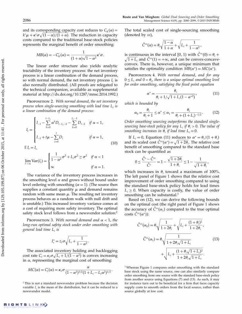
The proposition compares DSS with single-sourcingpolicies using a base-stock policy, but its messageextends to single-sourcing smoothing and the SCCpolicy (discussed in §3.4). Given that SCC cannot beoptimized analytically, we numerically optimized thesimulated cost under this policy and compared it tothe analytically optimized cost under the DSS policy.Figure 9 shows the magnitude of the cost reductionunder DSS relative to the cost under the SCC policy.With no sourcing cost advantage (�c = 0) and L= 1, theoptimal SCC policy (by definition) outperforms theDSS policy, but for moderate �c, DSS performs betterthan SCC. As �l rises, local capacity becomes moreconstrained and both the gain, and the domain whereDSS outperforms SCC, shrink.

4.5. Local and Global Capacity Costs(�l > 0 and �g > 0)

When both sources are capacitated, local and globalcapacity costs have counteracting effects on smoothingand offshoring as shown earlier in Proposition 8. Foran interior, dual-sourcing solution �∗ ∈ 40115 to exist,�c or �l must be sufficiently positive to offset a positive�g . Indeed, notice that if �g > 0 while �c = �l = 0, thecost is

C4�5= �g�L

√

1 −�

1 +�+

√

Ll +1

1 −�2≥ C4051

so that �∗ = 0 and LS is optimal. When �g > 0 and�c + �l > 0, there exist no general simple formulaeto express the optimal smoothing level. (Even whenL= 1, the FOC is a sixth order polynomial.) Even theLagrange solutions become exceedingly complex (andwe relegate them to the technical companion) but theydo suggest that the optimal solution is a function ofL�c +

√L�l and �g . However, given that �∗ decreases

as �g increases (Proposition 8), the exact solutions inthe previous section (only local capacity costs) provideupper bounds for the general case.

Additional results are found by approximating orbounding the marginal costs. For L= 1, a linear approx-imation of the FOC around � = 0 (light offshoring)yields

MB4�5 = �c + �g4−1 + 2�5+ �l + o4�5= MC4�5

= 41 +Ll5−1/2�+ o4�50

For L= 1, the marginal costs are also bounded:

MB405 = �c + �l − �g = 41 − �215

−3/2≤ MB4�∗5

= MC4�∗5≤ 41 −�∗25−3/20

A similar bounding can be done for L> 1, which yieldsthe following.

Dow

nloa

ded

from

info

rms.

org

by [

129.

105.

199.

87]

on 0

6 O

ctob

er 2

015,

at 1

1:41

. Fo

r pe

rson

al u

se o

nly,

all

righ

ts r

eser

ved.


Figure 9 (Color online) The Relative Value of Dual-Sourcing Smoothing Over Local Single-Sourcing-Capacitated SCC (Which Is the Optimal StrategyWhen �c = 0 and �l < 006, as Shown in the Left Panel); When the Global Source Has a Sourcing Cost Advantage (Right Panel), the DSS PolicyOutperforms SCC

0 0.2 0.4 0.6 0.8 1.00.8

1.0

1.2

1.4

1.6

1.8

2.0

2.2

Scal

ed c

ost DSS

SCC

LS

GS

00.1

0.20.3

0.40.5

0

0.2

0.4

0.60

2

4

6

8

L = 1

Rel

ativ

e va

lue

of D

SS (

%)

7.75%

�c�l

�l

�c = 0

Notes. L= 1, Ll = 0, �g = 0.

Proposition 13. Under normal demand, the followingbounds apply to the general case �i > 0:

1. For L = 1, if �c + �l − �g > 1, then the optimalsmoothing level and offshoring allocation has a lowerbound

�∗≥ �1 =

√

1 − 4�c + �l − �g5−2/3 (24)

that is asymptotically tight as �c + �l − �g → �. Other-wise, if 0 ≤ �c + �l − �g < 1 and �g <

12 :

�∗=

�c + �l − �g

41 +Ll5−1/2 − 2�g

+ o

(

�c + �l − �g

41 +Ll5−1/2 − 2�g

)

0 (25)

2. For any L > 1, if 44/43√

355�l − �g4e−1/2/25 ·

4L/√L− 15 > 1, then the optimal smoothing level has a

lower bound

�∗≥ �2 =

√

1 −

(

4

3√

3�l − �g

e−1/2

2L

√L− 1

)−2/3

0 (26)

Proposition 13 presents a useful lower bound forL= 1 that captures the three key parameters wherelocal and global capacity costs counteract each other (�land �g have opposite signs). The bound (26) shows thatthis counteraction extends to general L. Unfortunately,we have not been able to generate additional insightfulanalytic results.

Despite the limited tractability of the general case,Proposition 13 does shine a light on recent evolu-tions in global labor markets. A growing number ofAmerican companies are moving their manufacturingback to the United States because of higher Chineselabor costs. Although workers in developing Asiancountries are slowly acquiring more rights (increas-ing �g), there are signs that labor in rich countries is

becoming more flexible (decreasing �l) (The Economist2013). At the same time, The Economist reports thatEurope’s inflexible and costly labor markets, vis-à-visthe United States, is one of the reasons why reshoringis largely an American phenomenon (compared toEurope). Only when national government is makingthe business environment attractive enough, companieswill want to come back. Spurred by the Euro crisis,some European countries have now introduced sub-stantial labor-market reforms to remain competitive(e.g., western car workers are willing to work in nightshifts again). Our results predict that this will indeedwork in favor of backshoring work to the developedcountries.

5. Robustness and Comparison withOther Dual-Sourcing Policies

5.1. Robustness for Non-Normal DemandGiven that our analysis assumes normally distributeddemand, we want to understand how sensitive theresults are to this distributional assumption. Figure 10shows the optimal smoothing level �∗ for the uncapaci-tated and capacitated setting when demand follows agamma, lognormal, (discrete) geometric, and (contin-uous) uniform distribution, in comparison with theoptimal smoothing level assuming normal demand, �∗

N ,with identical average and CV. The functional depen-dence of �∗ on the standardized cost advantage or localcapacity cost follows that of the normally distributeddemand with identical CV. More importantly, the costdifference of a misestimate of �∗ in case of non-normaldemand is minimal (see Figure 11).

Dow

nloa

ded

from

info

rms.

org

by [

129.

105.

199.

87]

on 0

6 O

ctob

er 2

015,

at 1

1:41

. Fo

r pe

rson

al u

se o

nly,

all

righ

ts r

eser

ved.


Figure 10 (Color online) The Optimal Smoothing Level �∗ for Non-Normal Demand Follows the Optimal Smoothing Level �∗

N Assuming NormallyDistributed Demand with Identical Relative Uncertainty 4�g = 01 Ll = 05

� �

� �

�

��

��

��

�

�

��

��

� �

� �

Of course, the distributional assumptions are lessimportant as the variability decreases. Therefore, thereported cases not only give almost worst-case compar-isons, but given that the probability of negative demandexceeds 006% for CV exceeding 0.4, they also are push-ing the limit of the normal distribution assumption.Nevertheless, even with the assumed geometric dis-tribution (CV = 104), the analytic formulae (assumingnormal distribution) are still remarkably good approxi-mations. If average demand and standard deviationare scaled up in the conventional sense (as, e.g., inAllon and Van Mieghem 2010), we expect the appropri-ately scaled version of our results to be asymptoticallyoptimal. The scaled system with lead times is howevernontrivial and would be a research project in its own.

These results provide some numerical evidence thatour analysis remains valid to give guidance in thestrategic sourcing allocations in function of the finan-cial parameters, in practical settings regardless of thedistributional assumptions of the demand.

5.2. Performance of DSS Policy Compared toOther Dual-Sourcing Policies

In this section we compare the performance of thedual-sourcing smoothing policy with other existing

policies that have been shown to perform well in adual-sourcing setting.

The dual-base-stock policies are shown to be opti-mal in minimizing sourcing and inventory costs fora lead time difference L= 1 (Fukuda 1964) and nearoptimal for longer lead time differences (Veeraragha-van and Scheller-Wolf 2008, Scheller-Wolf et al. 2006).An important distinction is the state dimension: thesingle-index (SI) policy uses one state variable, beingthe total inventory position, whereas the dual-index(DI) policy tracks two state variables, i.e., the inventoryposition of the local source and the total inventoryposition to place, respectively, local and global orders.The vector-base-stock (VBS) policy keeps track of thelocal inventory position and the recently placed globalorders.

These policies have been shown to perform well ifonly sourcing and inventory costs are considered, andVeeraraghavan and Scheller-Wolf (2008), Scheller-Wolfet al. (2006) and Sheopuri et al. (2010) respectivelypresent efficient solution procedures to find the optimalbase-stock levels for the DI, SI, and VBS policies.However, they do not explicitly take into accountcapacity costs nor capacity flexibility. To minimize the

Dow

nloa

ded

from

info

rms.

org

by [

129.

105.

199.

87]

on 0

6 O

ctob

er 2

015,

at 1

1:41

. Fo

r pe

rson

al u

se o

nly,

all

righ

ts r

eser

ved.


Figure 11 (Color online) The Total Scaled Cost with Non-Normal Demand C4�∗5 Compared to the Scaled Cost Assuming the �∗

N Under Normal Demandwith Identical Relative Uncertainty 4�g = 01 Ll = 05

� �

� �

��

��

��

�

�

��

� �

� �

sum of average sourcing, inventory, and capacity costsper unit, as defined in (2), we therefore numericallyoptimized the target base-stock levels and the installedcapacities at each source. There is no general closed-form distribution for the orders and net inventory inthese policies (the global order may push the inventoryposition above its target level, causing an overshoot,so that no local order is placed), hence we resort tosimulation for performance analysis and optimization.

We also benchmark with the standing order, ortailored base-surge (TBS) policy, which is as well abase-stock-type policy: the global source supplies everyperiod a constant rate qg <�, and an additional order tothe local source is placed only when the inventory fallsbelow the target level. In the TBS policy, the standingorder may exceed the observed demand, resulting inexcess inventory excursions above its target level. Inessence, the “excess inventory process” behaves like aregulated random walk and the safety stock increasesas the standing order to the global source goes up(since the exponential tail of the regulated random walkwill be longer as qg increases). The TBS policy requiresthe evaluation of a G/D/1 queue, where the interarrivaltime has the per-period demand distribution and the

processing time is the fixed order size from the globalsource. For certain choices of the demand distribution,this is a tractable problem (as shown by Janakiramanet al. 2015), but for general demand distributions weneed to rely on a simulation analysis to optimize thetarget base-stock and capacity levels.

We conducted an extensive simulation study toanalyze the impact of capacity and lead time differencesin the uncapacitated and local capacitated setting(�g = 0 and Ll = 0). Figure 12 shows representativefindings, which can be summarized as follows:

(a) Without capacity costs (�l = �g = 0), DSS is outper-formed by the other dual-sourcing policies. This is to beexpected given that dual-base-stock policies are optimalin minimizing sourcing and inventory costs when L= 1,and near optimal for longer lead time differences. Theirperformance superiority derives from their ability toreact promptly to demand fluctuations. However, DSSis smoothing out the demand fluctuations in its orders(see Equation (9)); TBS is constrained by its standingglobal order but has dynamic local orders. Becauseof its smoothing behavior, DSS (and to a lesser extentTBS) needs more safety stock to act as a buffer betweenvolatile demand and smooth replenishments, leading

Dow

nloa

ded

from

info

rms.

org

by [

129.

105.

199.

87]

on 0

6 O

ctob

er 2

015,

at 1

1:41

. Fo

r pe

rson

al u

se o

nly,

all

righ

ts r

eser

ved.


Figure 12 (Color online) Scaled Cost Under Five Dual-Sourcing Policies Under Normal Demand 4�g = 01 Ll = 05

0 0.1 0.2 0.3 0.4 0.5 0.6 0.71.0

1.1

1.2

1.3

1.4

1.5

1.6

1.7

1.8Sc

aled

cos

t DSS

DI, SI, VBS

TBS

DSS

VBS

TBSDI, SI

L = 1�c = 0.1

L = 5�c = 0.1

�l

0 0.1 0.2 0.3 0.4 0.5 0.6 0.71.0

1.1

1.2

1.3

1.4

1.5

1.6

1.7

1.8

Scal

ed c

ost

�l

to increased inventory holding costs compared to thedual-base-stock policies. The TBS policy improves asthe lead time difference increases (as also shown byJanakiraman et al. 2015).

(b) With capacity costs, DSS can outperform the dual-base-stock policies because smoothing reduces bothlocal and global order variability and thus safety capac-ity requirements and costs. (Note that TBS completelysmoothens (levels) global orders and requires no globalbut more local safety capacity; the dual-base-stock poli-cies do not smooth at all and hence require higher localand global safety capacity.) This reduction in capacitycosts may compensate the increased inventory holdingcosts of smoothing. DSS outperforms the other policieswhen capacity costs are dominating: the higher thesourcing cost advantage �c, the more the capacity cost�l should dominate for DSS to outperform the otherpolicies. At the same time, the dual-base-stock policiesconverge naturally to global single sourcing when �lincreases, which may in turn outperform DSS (DSSdoes not naturally converge to single global sourcing).

(c) DSS performs best for longer lead time differencesL: DSS rapidly outperforms the other policies, evenfor low values of the capacity cost �l: in that case, thereduced capacity requirements quickly compensate forthe (relatively modest) increase in safety stocks due toorder smoothing.

These findings are valid under both normal and non-normal demand. Figure 13 illustrates the performanceof the DSS policy compared to these reference policiesunder a lognormal, (continuous) uniform, (discrete)geometric, and normal demand distribution. Thesedistributions are inspired by the abovementioned refer-ence papers in the dual-sourcing literature that usethe same distributions in their numerical experiments(Veeraraghavan and Scheller-Wolf 2008, Scheller-Wolfet al. 2006, Sheopuri et al. 2010).

In summary, DSS is a reasonable policy that is typi-cally competitive to the reference dual-sourcing policies

and can perform better in the presence of high capacitycosts and high lead time differences.

6. Summary and DiscussionThe main contribution of this paper is the inclusion ofcapacity cost and flexibility in a strategic global sourcingdecision, in addition to considering sourcing cost andlead times (as in the existing literature). We proposea linear control policy that performs well in both asingle- and dual-sourcing setting. An attractive featureof our analysis is the identification and analysis ofthree dimensionless parameters that, in addition to thelead times, are the four key forces behind the sourcingdecision: �c (which captures the financial trade-off, theinventory service level, the volatility in demand) and �land �g (which contain the ratio of capacity cost versusholding cost of, respectively, the local and global source,and their flexibility to work in overtime). These dataare typically available inside the firm (although onemay have to search for them in different departments),and we are now able to quantify how they contributeto strategic sourcing allocation decisions based on thesedata. These parameters also allow the comparison ofdifferent firms with different scales.

A numerical study shows that our analytic resultsfor normally distributed demand are robust for otherdistributions and that the smoothing policy is competi-tive to existing single- and dual-sourcing policies interms of total cost minimization. The study also con-firms expectations that the smoothing policy performsbetter in the presence of high capacity costs and highlead time differences given that it explicitly takes thecapacity costs and lead time difference into account.

As with any analytic study, ours begs for extensions.The assumption of normally distributed demand isessential in deriving all the analytical results: Directextensions could study demand distributions withhigher coefficients of variation (e.g., between one andtwo, or even up to three (Muckstadt 1997)), or with fat

Dow

nloa

ded

from

info

rms.

org

by [

129.

105.

199.

87]

on 0

6 O

ctob

er 2

015,

at 1

1:41

. Fo

r pe

rson

al u

se o

nly,

all

righ

ts r

eser

ved.


Figure 13 (Color online) Scaled Cost Under Five Dual-Sourcing Policies Under Normal and Non-Normal Demand 4�g = 01 Ll = 05

0 0.1 0.2 0.3 0.4 0.5 0.6 0.71.3

1.4

1.5

1.6

1.7

1.8

1.9

2.0

2.1

2.2

2.3

0.8

0.9

1.0

1.1

1.2

1.3

1.4

1.5

1.4

1.5

1.6

1.7

1.8

1.9

2.0

2.1

2.2

2.3

2.4

0 0.1 0.2 0.3 0.4 0.5 0.6 0.7

0 0.1 0.2 0.3 0.4 0.5 0.6 0.70 0.1 0.2 0.3 0.4 0.5 0.6 0.7

1.0

1.1

1.2

1.3

1.4

1.5

1.6

1.7

1.8Sc

aled

cos

tSc

aled

cos

t

Scal

ed c

ost

Scal

ed c

ost

DSS

DSS

DSSDSS

TBSTBS

TBS

SI

DI

DI, VBS

DI

DI

SI

SI

SI

VBS

VBS, TBS

VBS

NormalL = 2, �c = 0.1

LognormalL = 2, �c = 0.1

GeometricL = 2, �c = 0.1

UniformL = 2, �c = 0.1

�l �l

�l �l

tails, which we expect to favor more local sourcing,or with serial demand correlation, where negativecorrelation will favor smoothing and global sourcing.Another extension could analyze nonstationary demandpatterns to model, for example, how the sourcingallocation should adapt to the product life cycle.9

A third extension could insert unit cost or quantityuncertainty to model, for example, currency exchangerate risk or supply quality risk. Last, but not least,would be a game-theoretic multidecision-maker modelwhere one firm (the buyer) sources from one or twoindependent firms. These nonobvious model extensionsare full research projects themselves.

Supplemental MaterialSupplemental material to this paper is available at http://dx.doi.org/10.1287/mnsc.2014.1992.

Acknowledgments

9 One could apply our formula for each phase separately to predictthat the sourcing allocation will move from emphasizing local duringproduct introduction (low mean but high variability in demand) tooffshore during maturity and back to local during decline. However,this remains an unverified extrapolation of a stationary result.

The authors are indebted to Piet Van Mieghem for intro-ducing them to the Lagrange inversion theorem, and to theanonymous reviewers for their improvement suggestions.

Appendix. Lagrange’s Inversion Theorem andProof of Equation (19)Markushevich (1985, Vol. II, p. 88) gives Lagrange’s series forthe inverse of a complex function f 4z5 that is analytic aroundz0 with f ′4z05 6= 0 as

f −14z5 = z0 +

�∑

n=1

1n!

[

dn−1

dzn−1

(

z− z0

f 4z5− f 4z05

)n]∣∣

∣

∣

z=z0

· 4z− f 4z055n0 (27)

If f 4m54z05= 0 but f 4k54z05 6= 0 for all m< k, then (27) general-izes to Markushevich (1985, Vol. II, p. 92)

f −14z5 = z0 +

�∑

n=1

1n!

[

dn−1

dzn−1

(

z− z0

6f 4z5− f 4z0571/ks

)n]∣∣

∣

∣

z=z0

· 4z− f 4z055n/k1 (28)

where the subscript s denotes any fixed single-valued branchof the k-valued function 6f 4z5− f 4z057

1/k.

Dow

nloa

ded

from

info

rms.

org

by [

129.

105.

199.

87]

on 0

6 O

ctob

er 2

015,

at 1

1:41

. Fo

r pe

rson

al u

se o

nly,

all

righ

ts r

eser

ved.


If Ll = 0, consider the function f 4z5= z341 − z5m, whichis analytic in z because m= L− 2 ≥ 0 is integer. Given thatf ′405= f ′′405= 0 but f 435405= 3!> 0, (28) yields around z0 = 0:

dj

dzj41 − z5−n4m/35

∣

∣

∣

∣

z=0

=â44nm5/3 + j5

â44nm5/3541 − z5−4nm5/3−j

∣

∣

∣

∣

z=0

=â44nm5/3 + j5

â44nm5/351

and we obtain the Lagrange series for the inverse function,

f −14z5=

�∑

n=1

â4n4m/3 + 15− 15â44nm5/35

zn/3

n!1 (29)

where m= L− 2. (The technical companion shows that theradius of convergence is exactly � ≥ �L.) Here we were ableto calculate each term in the series explicitly due to thesimple form of f . If Ll > 0, the derivation becomes morecomplex but is still doable in closed form; with capacity costs,however, the derivation is term by term and cumbersome, asshown in the technical companion. �

ReferencesAllon G, Van Mieghem JA (2010) Global dual sourcing: Tailored base-

surge allocation to near- and offshore production. ManagementSci. 56(1):110–124.

Balakrishnan A, Geunes J, Pangburn MS (2004) Coordinating sup-ply chains by controlling upstream variability propagation.Manufacturing Service Oper. Management 6(2):163–183.

Bertrand JWM (1986) Balancing production level variations andinventory variations in complex production systems. Internat. J.Production Res. 24(5):1059–1074.

Bray RL, Mendelson H (2012) Information transmission and thebullwhip effect: An empirical investigation. Management Sci.58(5):860–875.

Cachon GP, Randall T, Schmidt GM (2007) In search of the bullwhipeffect. Manufacturing Service Oper. Management 9(4):457–479.

Cantor DE, Katok E (2012) Production smoothing in a serial supplychain: A laboratory investigation. Transportation Res. Part E48(4):781–794.

Chen L, Lee HL (2012) Bullwhip effect measurement and its implica-tions. Oper. Res. 60(4):771–784.

Combes F (2011) Inventory theory and mode choice in freighttransport: The case of the simultaneous use of two transportmodes on one shipper-receiver relationship. Working paper,Université Paris Est and Association for European Transportand Contributors, Paris.

Cui R, Allon G, Bassamboo A, Van Mieghem JA (2014) Informationsharing in supply chains: An empirical and theoretical valuation.Working paper, Kellogg School of Management, NorthwesternUniversity, Evanston, IL.

Economist, The (2013) Special report on outsourcing and offshoring:Here, there and everywhere. (January 19), http://www.economist.com/sites/default/files/20130119_offshoring_davos.pdf.

Forrester J (1961) Industrial Dynamics (MIT Press, Cambridge, MA).Fukuda Y (1964) Optimal policies for the inventory problem with

negotiable leadtime. Management Sci. 10(4):690–708.Galois É (1846) Oeuvres mathématiques d’Évariste Galois. J. des

Mathématiques Pures et Appliquées (11):381–444.George K, Ramaswamy S, Rassey L (2014) Next-shoring: A CEO’s

guide. McKinsey Quart. (January).Goel A, Gutierrez GJ (2011) Multiechelon procurement and dis-

tribution policies for traded commodities. Management Sci.57(12):2228–2244.

Graves SC (1988) Safety stocks in manufacturing systems. J. Manufac-turing Oper. Management 1(1):67–101.

Jain N, Girotra K, Netessine S (2014) Managing global sourcing:Inventory performance. Management Sci. 60(5):1202–1222.

Janakiraman G, Seshadri S, Sheopuri A (2015) Analysis of tailoredbase-surge policies in dual sourcing inventory systems. Manage-ment Sci. 61(7):1547–1561.

Lagrange J-L (1770) Nouvelle méthode pour résoudre les équationslittérales par le moyen des séries. Mémoires de l’Académie Royaledes Sciences et Belles-Lettres de Berlin (24):251–326.

Liu Z, Nagurney A (2013) Supply chain networks with globaloutsourcing and quick-response production under demand andcost uncertainty. Ann. Oper. Res. 208(1):251–289.

Magee JF (1958) Production Planning and Inventory Control (McGraw-Hill, New York).

Markushevich AI (1985) Theory of Functions of a Complex Variable,Vols. 1–3 (Chelsea Publishing, New York).

Muckstadt JA (1997) A paradigm lost. Technical Report 1180, Schoolof Operations Research and Industrial Engineering, CornellUniversity, Ithaca, New York.

Rosenshine M, Obee D (1976) Analysis of a standing order inventorysystem with emergency orders. Oper. Res. 24(6):1143–1155.

Scheller-Wolf A, Veeraraghavan S, van Houtum GJ (2006) Effectivedual sourcing with a single index policy. Working paper, TepperSchool of Business, Carnegie Mellon University, Pittsburgh.

Sheopuri A, Janakiraman G, Seshadri S (2010) New policies for thestochastic inventory control problem with two supply sources.Oper. Res. 58(3):734–745.

Simon H (1952) On the application of servomechanism theory in thestudy of production control. Econometrica 20(2):247–268.

Sobel MJ (1969) Production smoothing with stochastic demand I:Finite horizon case. Management Sci. 16(3):195–207.

Sobel MJ (1971) Production smoothing with stochastic demand II:Infinite horizon case. Management Sci. 17(11):724–735.

Tagaras G, Vlachos D (2001) A periodic review inventory systemwith emergency replenishments. Management Sci. 47(3):415–429.

Vassian HJ (1955) Application of discrete variable servo theory toinventory control. Oper. Res. 3(3):272–282.

Veeraraghavan S, Scheller-Wolf A (2008) Now or later: A simplepolicy for effective dual sourcing in capacitated systems. Oper.Res. 56(4):850–864.

Whittemore AS, Saunders SC (1977) Optimal inventory understochastic demand with two supply options. SIAM J. Appl. Math.32(2):293–305.

Wu X, Zhang F (2014) Home or overseas? An analysis of sourcingstrategies under competition. Management Sci. 60(5):1223–1240.

Zipkin P (2000) Foundations of Inventory Management (McGraw-Hill,New York).

Zipkin P (2008) Old and new methods for lost-sales inventorysystems. Oper. Res. 56(5):1256–1263.

Dow

nloa

ded

from

info

rms.

org

by [

129.

105.

199.

87]

on 0

6 O

ctob

er 2

015,

at 1

1:41

. Fo

r pe

rson

al u

se o

nly,

all

righ

ts r

eser

ved.

global dual sourcing and order smoothing: the impact of

Documents