global patterns of ecological productivity and … patterns of ecological productivity and tropical...

Global Patterns of Ecological Productivity and Tropical Forest Biomass

by

David Philip Martin Zaks

A thesis submitted in partial fulfillment of the requirements for the degree of

Master of Science Land Resources

Supported by the

Center for Sustainability and the Global Environment Gaylord Nelson Institute for Environmental Studies

at the

UNIVERSITY OF WISCONSIN-MADISON 2007

This work is licensed under the Creative Commons Attribution-Noncommercial-Share Alike 3.0 United States License. 2007.

Global Patterns of Ecological Productivity and Tropical Forest Biomass

By David Philip Martin Zaks

This thesis is approved for recommendation to the University of Wisconsin-Madison Graduate School

Advisor Title

Advisor Name Date

i

Acknowledgements

This thesis is the culmination of three years of coursework and research and acts

as the segue toward further sustainability science research. I am grateful to Jon Foley

who supported this research financially and intellectually. His hands-on style of advising

and encyclopedic knowledge and insight have greatly benefited this thesis and

development as a scientist. Navin Ramankutty, now at McGill University, and Carol

Barford also played an important role in this research. Navin gracefully introduced me to

the basic concepts of environmental modeling, and Carol's statistical and editorial finesse

greatly improved the research. I also thank Tom Gower and Dave Lewis, my committee

members. They gave me the freedom to independently conduct my research, yet gave

useful feedback when approached.

My colleagues and friends at the Center for Sustainability and the Global

Environment (SAGE) were instrumental in maintaining my intellectual and social sanity.

We traveled to San Francisco, Brazil and France, listened to practice presentations, and

shared food, drinks and experiences that have helped to shaped my experience at SAGE.

Finally, my friends and family in Madison and abroad have supported me in my

extracurricular activities that helped balance my life as a graduate student. From writing

and traveling to brewing and baking, someone from my network of friends was always

there to distract me from my research.

This work was supported by NASA Terrestrial Ecology grant (NAG5-13351).

iii

Abstract

Primary production is the process that results in the transfer of carbon dioxide

from the atmosphere to the biosphere. Patterns of primary production vary around the

globe and this thesis explores the climatic determinants of net primary productivity (NPP)

on a global scale and biomass accumulation across thee tropics. Scientists have been

collecting field measurements of these quantities for several decades and the studies

presented here use those measurements in addition to climate data to construct a suite of

empirical models of NPP and biomass accumulation.

From Miami to Madison: Investigating the Relationship Between Climate and Terrestrial Net Primary Production (Chapter 2) The 1973 "Miami Model" was the first global-scale empirical model of terrestrial net primary productivity (NPP), and its simplicity and relative accuracy has led to its continued use. However, improved techniques to measure NPP in the field and the expanded spatial and temporal range of observations have prompted this study, which reexamines the relationship of climatic variables to NPP. We developed several statistical models with paired climatic variables in order to investigate their relationships to terrestrial NPP. A reference data set of 3023 NPP field observations was compiled for calibration and parameter optimization. In addition to annual mean temperature and precipitation, as in the Miami Model, we chose more ecologically relevant climatic variables including growing degree-days, a soil moisture stress index, and photosynthetically active radiation (PAR). Calculated annual global NPP ranged from 36 to 74 Pg-C yr-1, comparable with previous studies. Comparisons of geographic patterns of NPP were made using biome and latitudinal averages.

Climatic and Edaphic Determinants of Aboveground Biomass Regrowth Rates in Tropical Forests (Chapter 3) The dynamics of tropical land-use / land cover change include deforestation, agricultural use, land abandonment and forest regrowth. Across the tropics the rate at which forests recover and sequester carbon is not fully understood. This study uses climate and soils data at the pan-tropical scale to model rates of aboveground biomass regrowth in tropical secondary forests. Data from primary literature studies across the tropics are used to fit

iv statistical models using biophysical variables, such as a forest climatic growth index and soil pH. Results are shown as biomass accumulation in tropical forests annually. Policy implications of re-growing forests are also discussed.

v

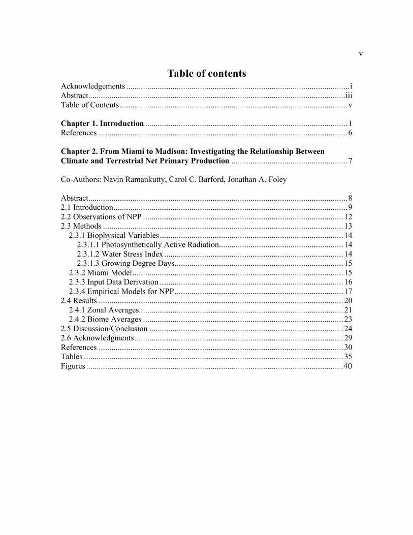
Table of contents Acknowledgements ..........................................................................................................i Abstract..........................................................................................................................iii Table of Contents ............................................................................................................v Chapter 1. Introduction ................................................................................................1 References ......................................................................................................................6 Chapter 2. From Miami to Madison: Investigating the Relationship Between Climate and Terrestrial Net Primary Production .......................................................7 Co-Authors: Navin Ramankutty, Carol C. Barford, Jonathan A. Foley Abstract...........................................................................................................................8 2.1 Introduction...............................................................................................................9 2.2 Observations of NPP ............................................................................................... 12 2.3 Methods .................................................................................................................. 13

2.3.1 Biophysical Variables ....................................................................................... 14 2.3.1.1 Photosynthetically Active Radiation........................................................... 14 2.3.1.2 Water Stress Index ..................................................................................... 14 2.3.1.3 Growing Degree Days................................................................................ 15

2.3.2 Miami Model.................................................................................................... 15 2.3.3 Input Data Derivation ....................................................................................... 16 2.3.4 Empirical Models for NPP................................................................................ 17

2.4 Results .................................................................................................................... 20 2.4.1 Zonal Averages................................................................................................. 21 2.4.2 Biome Averages ............................................................................................... 23

2.5 Discussion/Conclusion ............................................................................................ 24 2.6 Acknowledgments................................................................................................... 29 References .................................................................................................................... 30 Tables ........................................................................................................................... 35 Figures ..........................................................................................................................40

vi Chapter 3. Climatic and Edaphic Determinants of Aboveground Biomass Regrowth Rates in Tropical Forests ............................................................................................ 47 3.1 Introduction............................................................................................................. 49 3.2 Methods .................................................................................................................. 52 3.3 Results .................................................................................................................... 56 3.4 Discussion............................................................................................................... 58 3.5 Conclusions............................................................................................................. 61 Acknowledgements ....................................................................................................... 64 References .........................................................................................................................65 Tables ................................................................................................................................68 Figures ...............................................................................................................................70 Chapter 4. Conclusion................................................................................................. 81 References .................................................................................................................... 86

1

Chapter 1

Introduction

Since the beginning of the 20th century, an exponentially growing human

population has intensified resource demands and upset the balance of life on earth.

Elemental cycles, especially the carbon cycle, have been altered across the globe as

people modify the landscape to meet their needs and desires, based on capturing and

exploiting resources from natural ecosystems [Foley et al. 2005].

In recent years, an increasing amount of forest has been cleared for agriculture,

pasture and logging operations [Ramankutty and Foley, 1999]. These rapid changes

threaten rich stocks of biodiversity, carbon stores, water flows, climate and ultimately the

well-being of the inhabitants where these activities are taking place [Millennium

Ecosystem Assessment, 2005]. Most tropical forest-containing countries are also in the

process of developing their economic infrastructure. In the 20 years since the Brundtland

Commission brought the term "sustainable development" to the global community, we

still struggle to provide the basic needs of people now without compromising the needs of

future generations [World Commission on Environment and Development, 1987].

Humans rely on the services that ecosystems provide to fuel economies and

personal livelihoods. For example, a stable climate is needed to grow crops and maintain

a supply of fresh water, which not only is required for people directly, but also by plant

and animal populations. Background, or supporting services, including primary

production and soil formation are not directly consumed by people, but they are

2 necessary for the maintenance and production of other goods and services. Supporting

services, like primary production, lie at the base of a pyramid that supports many other

ecosystem functions, but are currently being undermined by human activity.

The importance of primary productivity lies in its many co-products including

carbon storage and release of oxygen through photosynthesis mediating the transfer of

water between the land and atmosphere through evapotranspiration and providing wood

products, food and fiber to people. Patterns of primary productivity are largely

determined by climate, but also influenced by soil, and topography amongst other factors.

From the hot and moist tropical forests to the cold and dry tundra of the northern

latitudes, temperature and precipitation (along with other biophysical variables) control

the stature and productivity of terrestrial ecosystems [Bonan, 2002]. It is this productivity

that supports the ecosystem goods and services provided by terrestrial landscapes.

Understanding the importance of primary productivity has long been the subject of

scientific inquiry.

Improving our understanding of primary production and supporting services is

one way address the problem of the environmental degradation which humans have

wrought on the Earth’s ecosystems. A series of studies have put forth a set of metrics to

estimate the amount of primary production used by humans, which has been calculated to

be between 23 and 40% [Vitousek et al. 1986; Haberl et al. 2002; Imhoff et al. 2004].

This staggering figure highlights the global impacts of our society, and also illustrates the

most effective ways of reducing our impacts while continuing to prosper. Studies

presented in this thesis advance the research on NPP by taking previously disparate field

studies and fusing them into a global model.

3 Previously conducted scientific studies of global environmental change provided

us a fragmented view of reality with small-scale studies that illustrated changes to

ecosystems on a limited basis [Reid et al. 2006]. The introduction of remote sensing

technology has given us a global view of the Earth, and is maturing to a point that will

eventually deliver real-time biophysical monitoring of the Earth. Until that time, the

network of field observations has to be leveraged to provide the needed data for regional

and global ecological studies.

This thesis presents two new additions to the growing body of carbon cycle

research. The second chapter presents an update to the Lieth [1978] model of global

terrestrial net primary productivity (NPP). The Lieth study used 50 observations to

correlate patterns of temperature and precipitation to NPP. In the 30+ years since that

study was published, a network of over 3,000 observations of NPP have been assembled.

The original model of temperature and precipitation is tested along with other, more

relevant climatic and biophysical variables, and presents a suite of global models of

terrestrial NPP.

In the third chapter, the question of NPP is narrowed from the global scale down

to a spatial focus on the pan-tropics. The research uses a network of observations of

forest biomass to construct a pan-tropical model of biomass accumulation during

regrowth. Similar to the NPP study, climatic variables are related to growth indices, but

in this study, only the biomass accumulation in tropical forests are included in the model.

Previous studies used a metric that related climate to biomass regrowth, and this

study incorporated more field data from the tropics, and also added a soil parameter to

differentiate fertile soils from poor soils. Results from this study can be coupled with

4 other studies to strengthen the decision-making abilities of tropical countries. With more

information about how tropical forests regrow after disturbance, better policy decisions

can be made when planning new protected areas, as areas of quick regrowth are more

valuable (in terms of carbon) than slower growing areas. The hot and wet conditions in

the tropics provide the right conditions for the dense forests that are home to an

abundance of plants, animals and people. The tropics contain over 40% [Dixon, 94] of

the terrestrial carbon and through conversion to non-forest uses, much is being released

into the atmosphere, furthering global warming and regional climatic changes.

While NPP measures the rate of carbon accumulation in vegetation, the carbon

content of vegetated land is reported as the total mass of live matter, of which the carbon

content of the biomass can easily be calculated. The NPP of a given area can depend on

its stage in the pathway of succession, as younger forests exhibit more vigorous growth,

and hence high NPP. Older forests balance the loss of fruits and seeds, respiration and

other maintenance functions with an NPP level that does not encourage growth, but

offsets other losses. Similarly, ecosystems exhibit different patterns of disturbance and

mortality, which on the short time scale can act to reduce biomass, but increase NPP as

vigorous regrowth is likely to happen with increased light in canopy gaps.

Field measurements of biomass and NPP use similar techniques. Biomass

measurements are reported in units of kg-C/m2, while NPP, as a flux, incorporates time

and is reported as kg-C/m2/yr. In forests, the most rigorous method of measuring biomass

is to randomly sample trees within a quadrant and destructively sample them (cut, dry

and weigh) to obtain the average biomass of a certain size class or area. These data can

then be used to create allometric equations that relate the height and diameter at breast

5 height (DBH) of a tree to its biomass. For NPP, successive measurements over time allow

for the growth of the tree and increase in height and DBH to be quantified, and the

growth over a certain interval of time to be reported. In most studies, both the NPP and

biomass are reported, and the data used in this study came from the published literature.

Large scale modeling exercises like these, and similar model validation studies

would be impossible to complete without the thousands of hours of field labor and lab

time devoted to understanding plot-scale ecosystem dynamics. While several data centers

have emerged to organize, conduct quality control and distribute ecological data, there

still remain inconsistencies in measurement methodologies, which can severely hamper

the ability for these diverse datasets to be combined. Standards for measurements of

often-measured quantities (i.e. NPP and biomass) should be created and implemented for

future field studies. New methodologies also need to be developed for quantities like

belowground NPP, which are currently tedious to measure and therefore often not

reported. Field ecological data are often used for validating algorithms for remote

sensing products. As these products become more pervasive in the field of ecology, the

importance of on-the-ground research should not be dismissed.

Building on past scientific studies, this thesis contributes new insights into global

ecosystem productivity and biogeochemical cycles. This kind of global ecological

science has a direct connection to the global policy with the ongoing work of the

Intergovernmental Panel on Climate Change, Kyoto Protocol and its successor. This new

empirical work highlights policy relevant science that can both aid in pushing the science

forward and guide a more sustainable development of the tropics.

6

References Bonan, G. B. (2002), Ecological climatology: concepts and applications, xi, 678 p. pp., Cambridge University Press, New York. Dixon, R. K., et al. (1994), Carbon Pools And Flux Of Global Forest Ecosystems, Science, 263, 185-190. Foley, J. A., et al. (2005), Global consequences of land use, Science, 309, 570-574. Haberl, H., et al. (2002), Human appropriation of net primary production, Science, 296, 1968-1969. Imhoff, M. L., et al. (2004), Global patterns in human consumption of net primary production, Nature, 429, 870-873. Lieth, H. (1978), Patterns of primary production in the biosphere, xv, 342 p. pp., Dowden distributed by Academic Press, Stroudsburg, Pa. Millennium Ecosystem Assessment (Program) (2005), Our human planet: summary for decision-makers, xv, 109 p. pp., Island Press, Washington, [D.C.]. Ramankutty, N., and J. A. Foley (1999), Estimating historical changes in global land cover: Croplands from 1700 to 1992, Glob. Biogeochem. Cycle, 13, 997-1027. Reid, W. V., and Millennium Ecosystem Assessment (Program) (2006), Bridging scales and knowledge systems: concepts and applications in ecosystem assessment, xii, 351 p., [354] p. of plates pp., Island Press, Washington. Vitousek, P. M., et al. (1986), Human Appropriation Of The Products Of Photosynthesis, Bioscience, 36, 368-373. World Commission on Environment and Development. (1987), Our common future, xv, 400 p. pp., Oxford University Press, Oxford; New York.

7

Chapter 2

From Miami to Madison: Investigating the Relationship Between Climate and Terrestrial Net Primary Production

David P.M. Zaks1, Navin Ramankutty2,1, Carol C. Barford1, Jonathan A. Foley1 1 Center for Sustainability and the Global Environment (SAGE) Nelson Institute for Environmental Studies University of Wisconsin 1710 University Avenue, Madison, WI 53726, USA

2 Department of Geography McGill University 805 Sherbrooke Street W., Montreal, QC, H3A 2K6, Canada Published in Global Biogeochemical Cycles, 2007

8

Abstract: The 1973 "Miami Model" was the first global-scale empirical model of terrestrial net

primary productivity (NPP), and its simplicity and relative accuracy has led to its

continued use. However, improved techniques to measure NPP in the field and the

expanded spatial and temporal range of observations have prompted this study, which

reexamines the relationship of climatic variables to NPP. We developed several statistical

models with paired climatic variables in order to investigate their relationships to

terrestrial NPP. A reference data set of 3023 NPP field observations was compiled for

calibration and parameter optimization. In addition to annual mean temperature and

precipitation, as in the Miami Model, we chose more ecologically relevant climatic

variables including growing degree-days, a soil moisture stress index, and

photosynthetically active radiation (PAR). Calculated annual global NPP ranged from 36

to 74 Pg-C yr-1, comparable with previous studies. Comparisons of geographic patterns

of NPP were made using biome and latitudinal averages.

9

2.1 Introduction: A key component of the terrestrial carbon cycle is net primary productivity

(NPP), the net rate at which plants assimilate carbon through photosynthesis and lose

carbon through autotrophic respiration [Clark et al., 2001a]. NPP also serves as an index

of energy flow through ecosystems [Roxburgh et al., 2004] and of ecosystem function

[Schlapfer and Schmid, 1999]. An improved understanding of the factors that determine

NPP can be valuable in reducing the level of uncertainty in the global carbon balance.

Moreover, knowledge about the spatial distribution of NPP across the globe is useful in

monitoring anthropogenic impacts on the terrestrial carbon cycle and associated changes

in the goods and services delivered by ecosystems [Cramer and Field, 1999; Haberl et al.,

2004; Meyerson et al., 2005; Vitousek et al., 1997].

NPP is a flux that cannot be observed directly, but is often modeled or

extrapolated from field measurements of other related quantities. NPP observations, as

referred to in this paper, are the relevant aboveground and belowground fluxes of organic

materials that are measured or estimated from field studies [Clark et al., 2001a; Gower et

al., 2001, 1999; Scurlock et al., 2002].While there is not yet a standardized methodology

for measuring NPP, this study assumes a relative amount of accuracy from figures

published in the literature. While observation-derived estimates are continuing to

accumulate across many regions of the world [Clark et al., 2001b; Malhi et al., 2004;

Olson et al., 2001; Scurlock et al., 1999], there is still no globally continuous data set of

observed NPP. Previous studies that estimated global patterns of NPP have ranged from

simple empirical models [Lieth, 1973; Lieth and Whittaker, 1975; Rosenzweig, 1968;

10 Whittaker and Likens, 1975] to fairly complicated process-based ecosystem models

[Cramer and Field, 1999; Foley, 1994; Foley et al., 1996; Haxeltine and Prentice, 1996;

Kucharik et al., 2000]. The simple logic of empirical models yields reasonable results,

but lacks mechanistic processes such as canopy and soil physics and plant physiology

utilized in process-based models [Foley et al., 1996; Kucharik et al., 2000; Running et al.,

2004; Sitch et al., 2003; Zhao et al., 2005]. Nevertheless, empirical models have proved

useful.

The Miami model [Lieth, 1973; Lieth and Whittaker, 1975] was one of the first

global empirical models; its simplicity and relative accuracy have led to its continued use.

It utilizes empirical functions of mean-annual temperature and annual precipitation fitted

to observations of NPP that were available in the early 1970s. The Miami model

determines NPP for a particular location as the minimum of the temperature and

precipitation functions. Hence there are no interactions between the two variables, and

temperature and moisture are not linked. This type of model must be reparameterized

with observation-based data if new sets of productivity and climate observations are used,

and therefore its usefulness in climate change studies is limited [Adams et al., 2004].

Nevertheless, its relative simplicity and ability to generate reasonable global patterns of

NPP is attractive. The empirical approach has proven effective in past studies, and here

we aim to provide updated global maps of NPP using more than 50 times as much data as

the original model.

Limited work has been done to test the control of multiple environmental

variables over global patterns of NPP [Adams et al., 2004]. In particular, it is well known

that plants respond to the seasonality of climate, and therefore it would be useful to

11 examine the relationship between NPP and biophysical variables that account for

seasonality. Moreover, the availability and quality of global-scale gridded climate data

has greatly improved since previous attempts to model NPP. New et al. [2002] have

developed finer spatial resolution climate data sets (10 minutes in latitude by longitude),

an improvement over previous data sets (0.5 to 5 degrees), allowing for a better match in

scale between the climate data sets and site-level NPP data. Finally, since the earlier work

of Lieth [1973] that used 52 field-based observations of NPP, the available data on NPP

has expanded to include thousands of sites from different climates and biomes.

In this paper, we develop a suite of empirical models in order to examine the

relationships between several ecologically related climatic variables and a global

compilation of 3023 observationally derived estimates of NPP for natural vegetation

types. These observations represent a range of climates, from hot and wet to cold and dry.

We further use the empirical model to spatially extrapolate the NPP observations to the

globe using observed global climate data. We explore potential environmental drivers of

NPP using process-based models of photosynthetically active radiation (PAR) to

represent light, growing degree-days (GDD) to represent seasonal heat accumulation, and

evapotranspiration or soil moisture to represent water availability.

These empirical global-scale NPP estimates may be used to improve

understanding of environmental controls on global-scale NPP, help understand how NPP

might have been altered by land use [e.g., DeFries et al., 1999], and assess the human

appropriation of net primary productivity [Cramer et al., 1999, 2001b; Haberl et al., 2004;

Vitousek et al., 1997]. In addition, comparing the resulting maps of this study with the

NPP output of process-based ecosystem models can assist in model development and

12 evaluation. Determining the current state of terrestrial productivity is also important for

global environmental agreements such as the Kyoto Protocol [Cramer et al., 2001a;

Steffen et al., 1998] and future climate-related polices [Benitez et al., 2007].

2.2 Observations of NPP The limited network of NPP observations has inhibited previous estimates and

models from coming to a consensus on the global distribution of NPP [Cramer and Field,

1999; Cramer et al., 1996; Scurlock et al., 1999]. Nevertheless, the development of

improved techniques to measure NPP in the field [Clark et al., 2001a; Gower et al., 2001,

1999; Scurlock et al., 2002] and the expanded spatial and temporal range of observations

has prompted our attempt to evaluate global-scale NPP patterns. A large reference data

set (n = 3023) of NPP field observations, including many from the Global Primary

Production Data Initiative [Olson et al., 2001], were compiled for this study.

Observations of NPP were gathered from the literature, with the majority from the

Oak Ridge National Laboratories (ORNL) Net Primary Production database (http://www

-eosdis.ornl.gov/NPP/npp_home.html), and additional studies to increase the spatial and

temporal coverage of the database (Table 1) [Malhi et al., 2004; Turner et al., 2005].

Observations from permanent pasture, crop, wetland, or other intensively managed sites

were omitted from this study; only "natural" ecosystems were included in the data set.

Data were plotted using their associated geographic coordinates, and sites that fell outside

of a land-sea mask were omitted from the study (Figure 2 in section 3.4). Observations

that were compiled in addition to the GPPDI were subject to the minimum requirements

set forth by Olson et al. [2001],

13 • "the use of one or more accepted methods to estimate above-or below-ground

NPP;

• specification of the geographical location for the study site;

• specification of the definition of biome or vegetation type; and

• a citable reference to peer-reviewed publication, symposium, or workshop

proceedings; book chapter; or technical memorandum."

Several sites (n = 393) reported only aboveground NPP. To estimate belowground NPP

for these sites, we used the relationships between aboveground and belowground NPP for

sites that reported measurements for both quantities reported by Olson et al. [2001]. A

belowground NPP to total NPP ratio of 0.50 was used for nonforest biomes, and a ratio of

0.22 was used for forest biomes. Gower et al. [1999] reported similar values, and the

forest/nonforest distinction was made by Olson et al. [2001] owing to a lack of statistical

difference in the ratios between biome functional types.

2.3 Methods The suite of models presented here expands on previous studies that illustrated

how climatic variables control patterns of net primary productivity [Churkina and

Running, 1998; King et al., 1997; Lieth, 1973; Post et al., 1997]. In this paper we develop

four different empirical models of NPP based on pairs of climate variables: (1) growing-

season averaged photosynthetically active radiation (PAR) and a water stress index, (2)

growing degree-day (base 5) and a water-stress index, (3) annual mean temperature and

total annual precipitation, the variables and functional form used by Lieth [1973], and (4)

a modified version of the Lieth [1973] model.

14

2.3.1 Biophysical Variables

2.3.1.1 Photosynthetically Active Radiation Light use efficiency models [Montieth, 1972, 1977] are based on the principle that

canopy carbon fixation is proportional to absorbed light [McCree, 1972] and have been

shown to be effective in modeling NPP [Gower et al., 1999; Ruimy et al., 1999]. We use

the annual average incident photosynthetically active radiation (PAR) summed for every

day that the average temperature is greater than 0°C. Adjusting PAR for times when

temperatures lie above zero allows consideration of high-altitude areas, where

temperatures can differ significantly from other sites at the same latitude. Preliminary

analyses using our 3023 observations suggested a linear relationship between PAR and

observed NPP.

2.3.1.2 Water Stress Index Water availability is crucial to vegetation growth [Stephenson, 1990].

Rosenzweig [1968] was the first to use actual evapotranspiration, a surrogate for moisture

availability, to model NPP. Most global ecosystem models use evapotranspiration (either

potential or actual) as a key element in computing the water balance [Churkina et al.,

1999]. Potential evapotranspiration is the rate at which evapotranspiration would occur if

the soil was always wet, while actual evapotranspiration is a measure of the actual

amount of water that either transpires or evaporates from plants and soil [Churkina et al.,

1999; Rosenzweig, 1968; Stephenson, 1998]. Here we employ a water stress index

(defined as actual evapotranspiration divided by potential evapotranspiration) to gauge

15 the ability of the land surface to satisfy the evaporative demands of the atmosphere [e.g.,

Prentice et al., 1993; Foley, 1994]. Initial data analysis suggested a linear relationship

between available water and NPP.

2.3.1.3 Growing Degree Days Growing degree-days (GDD) are often used as a surrogate to represent the length

and thermal properties of the growing season[Cramer and Solomon, 1993]. A sufficient

amount of heat during the growing season is required to drive photosynthesis reactions

[Bonan, 2002]. The response function for GDD was designed to simulate these

physiological constraints and is prescribed as a sigmoidal curve, as suggested by a

preliminary analysis of GDD versus NPP.

2.3.2 Miami Model The Miami model is based on relationships between annual average temperature,

annual precipitation, and NPP. The function that describes the relationship between

precipitation and productivity is based on the Walter ratio, where the NPP for arid

regions was observed to increase by 1.0 g-C m-2 for each millimeter of precipitation

[Lieth, 1973]. The temperature model is based on the van’t Hoff rule, which states that

productivity doubles every 10°C between -10°C and 20°C [Lieth, 1973]. Over the past 30

years, this model has been used as a baseline data set and has been shown to yield

"reasonable estimates" of global patterns of productivity [Adams et al., 2004].

16 2.3.3 Input Data Derivation The biophysical variables were calculated using a simple energy and water balance model

[Foley, 1994; Haxeltine and Prentice, 1996; Prentice et al., 1993; Ramankutty et al.,

2002].

Growing degree-days (GDD) were calculated as

!

GDD = max(0,Ti " 5)i=1

365

# (day-degrees) (1)

where Ti is the daily mean temperature that is set to a (base temperature,5°C), summed

over the year.

The potential evapotranspiration (PET) was calculated as

!

PET = Rn0 " * s (s+ #) (mm/day) (2)

Rn0 is the daily net radiation, s is the rate of change of saturated water-vapor pressure

with respect to temperature, γ is the psychrometer constant (65 Pa/K) and λ is the latent

heat of vaporization of water (2.5 x106 J/kg).

Following the approach of Prentice et al. [1993], actual evapotranspiration (AET) was

calculated as

!

AET =min(PET,ETmax (Sm /WCa)) (mm/day) (3)

where Sm is soil moisture, WCa is available water content, and ETmax is the maximum

daily evapotranspiration, 5.0 (mm/day).

17

A water stress index (WSI), indicating the ability of the land surface to meet the

atmospheric demand for water, was calculated as

!

WSI = AET /PET (unit less) (4)

and is a measure of water availability to plants.

The average incident photosynthetically active radiation (PAR) was summed

during the growing season, which is defined as every day with an average temperature

greater than zero.

Observed monthly mean climate data were entered in the model at 10' (0.1667°)

latitude x longitude spatial resolution, an improvement over previous climate data sets

[New et al., 2002]. The monthly mean input values are interpolated to accommodate the

dailytime step of the model, except for evapotranspiration, which is calculated on a

quasihourly time step. The model was run for 50 years to ensure that an equilibrium state

was reached in the water balance submodel. The results for GDD5, WSI, and PAR are

shown in Figures 1a – 1c. The mean annual temperature and annual precipitation values,

also derived from New et al. [2002], are shown in Figures 1d and 1e.

2.3.4 Empirical Models for NPP We developed statistical models between pairs of the biophysical variables and

observations of NPP, as follows:

18

!

NPP(PAR,WSI) =max(0,(a*PAR + b*WSI " c)) (5)

!

NPP(GDD5,WSI) =max(0,((a /(1+ exp(b " c *GDD5))* (d *WSI " e))) (6)

!

NPP(Temp,Precip) = ((a /1+ exp(b " c *Temp))* (d * (1" exp(e*Precip)))) (7)

!

NPP(Temp,Precip) =min((a /1+ exp(b " c *Temp)),(d * (1" exp(e*Precip)))) (8)

The empirical functions were designed to be linear with PAR and WSI and

sigmoidal with GDD. These equations were constrained to ensure NPP values greater

than zero. The temperature-precipitation model (equation (7)) used the same functional

form for each variable individually as Lieth [1973], but uses a multiplicative form, rather

than finding the limiting criterion, to combine them; this form fits the model over a

surface using both independent variables. The original Miami model formulation

(equation 8) was also used with updated coefficients.

We then fit these equations to the observed NPP data. Unfortunately, the

distribution of NPP observations is clustered in geographic in the Northern Hemisphere

temperate latitudes and few observations in the Southern Hemisphere (Figure 2).

Furthermore, within each of the 100 grid cells of the input climate data, observed NPP

varies in response to changes in microclimate, soil heterogeneity, and other factors.

Ideally, functions would be fit through the entire cloud of data points, but the

aforementioned variability does not allow for a good model fit. Therefore we developed a

scheme to aggregate NPP observations in climate space and explicitly remove the

microscale variability in NPP observations.

19 NPP observations into a 10 x 10 matrix that described the range of climatic

variables across the globe. Each axis represented one of the independent climate variables

and was divided into 10 bins of equal size (Figures 3a3c). The input climate data and

observations were scaled from 0.0 to 1.0 to aid in the modeling process, and all model

coefficients are given in scaled terms. NPP observations were overlaid with the 100

resolution biophysical data and assigned to the grid. Few NPP observations were

measured in extreme environments where NPP is known to be very low (i.e., deserts).

Therefore, to allow the empirical model to fit accurately at low NPP values, "dummy"

bins were added to the matrix where one of the climate variables was zero, and a value of

zero NPP was assigned to these bins.

The wide range of taxa and biological responses to climate in each climate bin, in

addition to other uncertainties, add to the variability in the median NPP value in each bin.

Comparing the mean across all the bins of the within-bin standard deviation to the

standard deviation of the median of all the climate bins revealed that about half the total

variance contained in the within-bin variability (Table 2). This study does not try to

explain the within-bin variance, but rather focuses on the broad-scale relationship

between NPP and climate.

The model coefficients were determined using a converging successive

approximation approach, whereby we bisected the parameter space of each coefficient

and in each iteration determined the best solution, then repeated the procedure to further

refine the parameter space. Model fitting was initialized using coefficient values chosen

to minimize variance in the final model output. Binned observed NPP was compared to

the model output for each fitting iteration, and fits yielding acceptable slope (0.9 < slope

20 < 1.1) and intercept (0 < intercept < 0.2) in predicted versus observed (1:1) plots were

ranked according to minimization of the least squares error (Table 3). The best fitting set

of coefficients was then used to update the range of acceptable values for the next fitting

iteration. One hundred iterations were performed, which was sufficient for a fit to

converge on stable values.

Each model fit was then used in one of 500 bootstrap simulations of global NPP

to determine the uncertainty of modeled NPP estimates. For each model fit, the original

data set of 3023 observations was randomly sampled with replacement and then binned

as described above. For each 10' grid cell, the median NPP value from the bootstrap

analysis is reported (Figures 4a – 4d). The 90% confidence intervals from the Monte

Carlo analyses are used for further model comparisons. Global NPP values and their 90%

confidence intervals for each model type were calculated by summing the output of each

of the model fits over the globe, then ranking the 500 sums and choosing the 5th

percentile, median and 95th percentile values.

2.4 Results The modeled spatial patterns of NPP were compared to observations in order to

evaluate the overall goodness of model fit. Data-poor areas, where it was impossible to

validate the model, include much of the African continent, the Middle East, southern

South America, western Canada, India, northern Russia, western Australia, and Southeast

Asia. While we were unable to evaluate model performance over these data-poor regions,

enough observations were available elsewhere for a thorough evaluation of goodness of

fit.

21 Modeled values of NPP ranged from 0 to 1577 g-C m-2 yr-1 across the three

models, and the global total NPP from the median model values ranged from 41.8 to 61.3

Gt-C yr-1 (Table 4), which falls within the range reported by other studies summarized by

Cramer et al. [1999]. In general, modeled values of NPP were highest in humid tropical

forests, where neither water nor heat limits production. The lowest modeled values of

NPP were in the desert and polar regions where sufficient quantities of water, heat or

light are not available for plant production.

A histogram of productivity by area illustrates the general patterns of global NPP

(Figure 5). All the models produced nonnormal frequency distributions of NPP, with

more low-productivity area and less high productivity area. There are comparatively few

low NPP values in the PAR/ WSI model, while more area is occupied by the midrange

values (400 – 800 g-C m-2 yr-1). The Temp/Precip (Miami) generally has higher values

than the Temp/Precip (multiplicative) model although its maximum NPP value is only

1100 g-C m-2 yr-1. This nonspatially explicit interpretation of global NPP is

complemented by the biome and zonal averages.

2.4.1 Zonal Averages The observations and model results were sorted into 2.5° latitude bands and

averages for each were calculated for those that contained greater than five observations

(Figure 6a). Observations cover the range of 47.5° to 75°, while the land surface extends

from 55° to 85°. When comparing observations to modeled NPP using zonal aver ages,

the widely distributed network of points allows for comparison to modeled results. Zonal-

average model results follow the general latitudinal trends of the observations, with NPP

22 decreasing from the equator to the poles. In most areas, the models simulated the

observations well, but in other areas, the patterns of modeled NPP differed from the

expected results. We believe that this is simply a result of the insufficient spatial

coverage of the observations.

The observations around 40° are dominated by a cluster of points in New Zealand

and southern Australia that report NPP values higher than expected for the region. Most

of these observations come from the temperate broadleaf evergreen and grassland

biomes. In addition, there are no other observations in that latitude band, therefore the

unexpectedly high observations are not moderated by lower values that would be found at

that latitude in South America.

All models exhibited peak NPP values at the equator, however, observed data

decreased from both -2.5° and 2.5° to 0°. While observations in this latitude band did not

correspond to the modeled NPP, there were likely other observations in the same climate

matrix cell that acted to increase the modeled NPP values for this area. Averaging grid

cells over 2.5° latitude bands for the whole land surface allows for comparison of general

trends between models (Figure 6b). NPP for all models exhibited a trimodal distribution

consistent with other studies [Kicklighter et al., 1999].

The slight peak in NPP at -55° corresponds to the very southern tip of South

America, where there is sufficient light and water for plant growth. Other latitude bands

were averaged over larger areas, and this slight peak can be attributed to the small land

area in this band. All models increase to their peak NPP at the equator. The PAR/WSI

model has the lowest peak, and this can be attributed to a reduction in PAR due to an

increase in cloud cover, and hence, a decrease in NPP. All models decrease from their

23 peaks at the equator, as deserts dominate the land surface around 20°. The PAR/WSI and

GDD/WSI models increase in NPP and peak at 55° as the water availability and PAR or

GDD are sufficient for plant growth, but the Temp/Precip model NPP declines in

magnitude until 90°.

2.4.2 Biome Averages A classification of global vegetation biomes by Ramankutty and Foley [1999]

defined 15 biomes on the basis of potential natural vegetation. The quartiles for the

observations of NPP by each biome are displayed along with our NPP model estimates

for grid cells that contain observations (Figure 7a) and over the whole land surface

(Figure 7b). Bounds of the 90% confidence intervals (5th and 95th percentiles) in the

modeled NPP are shown for each biome. There are no observations from the polar desert/

rock/ice biome, and therefore it is not included in the figures. NPP tends to be higher in

the forested biomes, with the highest zonal averages occurring in the tropical forest

biomes, followed by the temperate forest biomes. The lowest modeled NPP values occur

in nonforest biomes: open shrubland, tundra, and desert.

Model output falls within the bounds of the observations for most biomes. In the

boreal deciduous forest/ woodland and tundra biomes, both forms of the Temp/ Precip

model underpredicts NPP, as they generally predict low values in northern latitudes. The

GDD/WSI model underpredicts NPP in the desert biome. This can be attributed to the

functional form of the equation, and NPP is modeled to be zero in most high-latitude and

desert areas.

24 In both tropical biomes, the PAR/WSI model returns the lowest NPP. In the three

temperate biomes the PAR/WSI model reports the highest NPP, and in most cases, the

Temp/ Precip models report the lowest values. In the nonforest biomes, the general trend

(from highest NPP to lowest) is PAR/WSI, GDD/WSI,Temp/Precip

(Miami),Temp/Precip (multiplicative).

When NPP is averaged across the entire land surface, the general trends remain

constant, with the exception of a few biomes (Figure 7b). In general, when averaged over

a larger area, the magnitude of NPP is lower for all biomes, when compared to averaging

only over grid cells with observations. With the exception of the boreal biomes, forested

biomes have higher NPP than nonforest biomes.

2.5 Discussion/Conclusion Net primary production is one of the fundamental characteristics of the biosphere,

providing usable energy for life on Earth. However, our knowledge of the geographic

patterns of NPP around the planet is still limited. Advancements in field measurements of

NPP and associated biophysical variables over the last several decades have allowed for

models of biospheric processes to be developed and tested. In this paper, we have

demonstrated that global patterns of NPP can be reasonably predicted using empirical

models based on simple pairs of biophysical and climatic variables. These models allow

us to gain an understanding of the global patterns of NPP.

While there is still a great deal of variability, all the models performed within

expected bounds with respect to global totals of NPP and spatial distribution across

biomes and latitude zones. The PAR/WSI and GDD/WSI models seem to represent most

25 closely the physiological limitations on plants that ultimately affect their NPP. The

Temp/Precip models, used to retest the hypothesis of Lieth [1973], also captured the

drivers of global-scale NPP.

While our study has taken a step forward in developing models of global patterns

of NPP, there are still many caveats that need to be addressed. First, observations of NPP

in the field are plagued by numerous problems. Some authors have pointed to

inconsistencies in the functional definition of NPP [Roxburgh et al., 2005], while others

have criticized the "incomplete or inappropriate" methods of field measurement [Clark et

al., 2001a]. NPP is most commonly reported as an annual flux, and those measurements

are difficult to obtain, even over small areas[Cramer et al., 2001a]. Clark et al. [2001a]

argued that in situ NPP calculations (for forests) should be based on the aggregation of

above and below ground coarse woody increment in addition to litterfall, insect damage,

fruit production, and root exudates. However, the time and money required to collect data

of that quality over a large spatial scale are prohibitive. In addition, early estimates of

NPP, such as those from the International Biosphere Programme (IBP) used less

sophisticated methodologies and may underestimate both above and belowground stocks

of carbon [Clark et al., 2001a].

There is also a discrepancy between the scale of our model simulations and the

NPP observations. The size of a 100 grid cell at the equator is 345 km2, while the average

size of a field study is often several hectares or less. Local observations of NPP are

influenced by landscape heterogeneity, including changes in microclimate and soil

fertility due to land use, historical patterns of disturbance, successional stage, altitudinal

26 gradients, and hydrology. Using a Monte-Carlo analysis allowed for calculation of

confidence intervals of the median NPP value for each grid cell.

Another obstacle of using such a large and diverse database of observations is the

time period in which the observations have been taken. From the IBP studies of the 1960s

– 1970s to the most recent MODIS BigFoot validation efforts from 1999 – 2003, both

atmospheric carbon dioxide concentrations and global patterns of climate have changed

[Intergovernmental Panel on Climate Change, 2001]. These changes have the potential to

impact the physiological and ecological responses of plants, making the observations of

NPP from different time periods functionally incompatible. The climate data used by

New et al. [2002] to derive the biophysical variables are 30-year averages (1961 – 1990)

and do not cover the full time range of the observations.

In order to quantify NPP over large spatial scales, methods beyond direct

observation must be used. Several space-borne sensors (i.e., MODIS, AVHRR, Landsat)

record reflectance values from vegetation that can be processed, through biophysical

models like those described here, to estimate NPP [Bradford et al., 2005; Goetz and

Prince, 1996; Turner et al.,2005]. However, the raw reflectance data must still be

calibrated to on-the-ground measurements in order to train the algorithms, as reflectance

is not a direct measurement of productivity. Flux tower measurement sites also report

NPP [Hibbard et al., 2005], but the methods of standardization for these sites is ongoing

and their spatial distribution is too limited for incorporation into this study.

While the general patterns of NPP were similar between the four models, the

magnitude and distribution varied sufficiently to warrant further investigation. The

mathematical form of the model equations had some unintended consequences when

27 applied globally. In the models that used sigmoidal equations, even if the independent

variable was zero, modeled NPP would nevertheless have a small positive value. For

example, if a grid cell had zero growing-degree days, NPP would still never be exactly

zero. In addition, in the models that used the water stress index, the linear form of the

equation included an intercept that produced negative NPP for highly water stressed

areas; in these cases the model would predict a negative NPP, but was constrained to

have values of zero or higher.

This study reports the potential NPP of the world’s "natural" ecosystems and

excludes managed areas such as crops, pastures, and plantations. The NPP of modified

landscapes can vary dramatically owing to irrigation, fertilization, grazing, and other

alterations to natural systems. NPP of such systems has been calculated [Hicke and

Lobell, 2004; Prince et al., 2001] in a broader attempt to determine the human impact on

the biosphere [Imhoff et al., 2004; Vitousek et al., 1997].

The Miami model [Lieth, 1973] was a major achievement in understanding global

patterns of productivity, but more observations and new hypotheses about the climatic

controls on NPP call for reanalysis of the problem. We developed four empirical models

in order to extend a finite database of NPP observations to describe global patterns of

NPP. We found that the PAR/WSI model performed the best, followed by the GDD/WSI

and Temp/ Precip models.

This study strengthens our understanding of global productivity and will allow for

improved ecosystem model evaluation. Standardization of field measurement techniques

to quantify changes in ecosystem productivity and functioning is needed, in addition to a

greater number of study sites. Further work on incorporating these global networks of

28 field measurements into global ecosystem models could help reduce uncertain ties in our

understanding of the biospheric response to land use and changing climate.

29

2.6 Acknowledgments We would like to thank C. Kucharik, S. Olson, and E. Sowatzke for their support. This

work was supported by NASA Terrestrial Ecology grant (NAG5-13351). Supplemental

material will be posted at http://www.sage.wisc.edu.

30

References Adams, B., A. White, and T. M. Lenton (2004), An analysis of some diverse approaches to modelling terrestrial net primary productivity, Ecol. Modell., 177, 353 – 391. Benitez, P. C., I. McCallum, M. Obersteiner, and Y. Yamagata (2007), Global potential for carbon sequestration: Geographical distribution, country risk and policy implications, Ecol. Econ., 60(3), 572 – 583. Bonan, G. B. (2002), Ecological Climatology: Concepts and Applications, 678 pp., Cambridge Univ. Press, New York. Bradford, J. B., J. A. Hicke, and W. K. Lauenroth (2005), The relative importance of light-use efficiency modifications from environmental conditions and cultivation for estimation of large-scale net primary productivity, Remote Sens. Environ., 96, 246 – 255. Churkina, G., and S. W. Running (1998), Contrasting climatic controls on the estimated productivity of global terrestrial biomes, Ecosystems, 1, 206 – 215. Churkina, G., S. W. Running, and A. L. Schloss (1999), Comparing global models of terrestrial net primary productivity (NPP): The importance of water availability, Global Change Biol., 5, 46 – 55. Clark, D. A., S. Brown, D. W. Kicklighter, J. Q. Chambers, J. R. Thomlinson, and J. Ni (2001a), Measuring net primary production in forests: Concepts and field methods, Ecol. Appl., 11, 356 – 370. Clark, D. A., S. Brown, D. W. Kicklighter, J. Q. Chambers, J. R. Thomlinson, J. Ni, and E. A. Holland (2001b), Net primary production in tropical forests: An evaluation and synthesis of existing field data, Ecol. Appl., 11, 371 – 384. Cramer, W., and C. B. Field (1999), Comparing global models of terrestrial net primary productivity (NPP): Introduction, Global Change Biol., 5, III – IV. Cramer, W., and A. Solomon (1993), Climatic classification and future global redistribution of agricultural lands, Clim. Res., 3, 97 – 110. Cramer, W., B. Moore, and D. Sahagian (1996), Data needs for modelling global biospheric carbon fluxes: Lessons from a comparison of models, IGBP Newsl., 27, 13 – 15. Cramer,W., D. W.Kicklighter,A.Bondeau,B.Moore, C. Churkina, B. Nemry, A. Ruimy, and A. L. Schloss (1999), Comparing global models of terrestrial net primary productivity (NPP): Overview and key results, Global Change Biol., 5, 1– 15.

31 Cramer, W., et al. (2001a), Global response of terrestrial ecosystem structure and function to CO2 and climate change: Results from six dynamic global vegetation models, Global Change Biol., 7, 357 – 373. Cramer, W., R. J. Olson, S. Prince, J. M. O. Scurlock, and Members of the Global Primary Production Data Initiative (2001b), Determining present patterns of global productivity, in Terrestrial Global Productivity, edited by J. Roy, B. Saugier, and H. A. Mooney, pp. 429 – 448, Academic Press, San Diego, Calif. DeFries, R. S., C. B. Field, I. Fung, G. J. Collatz, and L. Bounoua (1999), Combining satellite data and biogeochemical models to estimate global effects of human-induced land cover change on carbon emissions and primary productivity, Global Biogeochem. Cycles, 13, 803 – 815. Foley, J. A. (1994), Net primary productivity in the terrestrial biosphere: The application of a global model, J. Geophys. Res., 99,20,773– 20,783. Foley, J. A., I. C. Prentice, N. Ramankutty, S. Levis, D. Pollard, S. Sitch, and A. Haxeltine (1996), An integrated biosphere model of land surface processes, terrestrial carbon balance, and vegetation dynamics, Global Biogeochem. Cycles, 10, 603 – 628. Goetz, S. J., and S. D. Prince (1996), Remote sensing of net primary production in boreal forest stands, Agric. For. Meteorol., 78, 149 – 179. Gower, S. T., C. J. Kucharik, and J. M. Norman (1999), Direct and indirect estimation of leaf area index, f (APAR), and net primary production of terrestrial ecosystems, Remote Sens. Environ., 70, 29 – 51. Gower, S. T., O. Krankina, R. J. Olson, M. Apps, S. Linder, and C. Wang (2001), Net primary production and carbon allocation patterns of boreal forest ecosystems, Ecol. Appl., 11, 1395 – 1411. Haberl, H., et al. (2004), Human appropriation of net primary production and species diversity in agricultural landscapes, Agric. Ecosyst. Environ., 102, 213 – 218. Haxeltine, A., and I. C. Prentice (1996), BIOME3: An equilibrium terrestrial biosphere model based on ecophysiological constraints, resource availability, and competition among plant functional types, Global Biogeochem. Cycles, 10, 693 – 709. Hibbard, K. A., B. E. Law, M. Reichstein, and J. Sulzman (2005), An analysis of soil respiration across Northern Hemisphere temperate ecosystems, Biogeochemistry, 73, 29 – 70.

32 Hicke, J. A., and D. B. Lobell (2004), Spatiotemporal patterns of cropland area and net primary production in the central United States estimated from USDA agricultural information, Geophys. Res. Lett., 31, L20502, doi:10.1029/2004GL020927. Imhoff, M. L., L. Bounoua, T. Ricketts, C. Loucks, R. Harriss, and W. T. Lawrence (2004), Global patterns in human consumption of net primary production, Nature, 429, 870 – 873. Intergovernmental Panel on Climate Change (2001), Climate Change 2001: Synthesis Report. A Contribution of Working Groups I, II, and III to the Third Assessment Report of the Intergovernmental Panel on Climate Change, edited by R. T. Watson and D. L. Albritton, 397 pp., Cambridge Univ. Press, New York. Kicklighter, D.W., A. Bondeau, A. L. Schloss, J. Kaduk, and A. D. McGuire (1999), Comparing global models of terrestrial net primary productivity (NPP): Global pattern and differentiation by major biomes, Global Change Biol., 5, 16 – 24. King, A. W., W. M. Post, and S. D. Wullschleger (1997), The potential response of terrestrial carbon storage to changes in climate and atmospheric CO2, Clim. Change, 35, 199 – 227. Kucharik, C. J., J. A. Foley, C. Delire, V. A. Fisher, M. T. Coe, J. D. Lenters, C. Young-Molling, N. Ramankutty, J. M. Norman, and S. T. Gower (2000), Testing the performance of a Dynamic Global Ecosystem Model: Water balance, carbon balance, and vegetation structure, Global Biogeochem. Cycles, 14, 795 – 825. Lieth, H. (1973), Primary production: Terrestrial ecosystems, Human Ecol., 1, 303 – 332. Lieth, H., and R. H. Whittaker (1975), Primary Productivity of the Biosphere, 339 pp., Springer, New York. Malhi, Y., et al. (2004), The above-ground coarse wood productivity of 104 Neotropical forest plots, Global Change Biol., 10, 563 – 591. McCree, K. J. (1972), The action spectrum, absorption, and quantum yield of photosynthesis in crop plants, Agric. Meteorol., 9, 191 – 216. Meyerson, L. A., J. Baron, J. M. Melillo, R. J. Naiman, R. I. O’Malley, G. Orians, M. A. Palmer, A. S.P. Pfaff, S. W. Running, and O. E. Sala (2005), Aggregate measures of ecosystem services: Can we take the pulse of nature?, Front. Ecol. Environ., 3, 56 – 59. Montieth, J. (1972), Solar radiation and productivity in tropical ecosystems, J. Appl. Ecol., 9, 747 – 766.

33 Montieth, J. (1977), Climate and efficiency of crop production in Britain, Philos. Trans. R. Soc., Ser. B, 281, 277 – 294. New, M., D. Lister, M. Hulme, and I. Makin (2002), A high-resolution data set of surface climate over global land areas, Clim. Res., 21, 1– 25. Olson, R. J., K. Johnson, D. L. Zheng, and J. M. O. Scurlock (2001), Global and regional ecosystem modeling: Databases of model drivers and validation measureme nts, ORNL/TM-2001/196, 95 pp., Environ. Sci. Div., Oak Ridge Natl. Lab., Oak Ridge, Tenn. Post, W. M., A. W. King, and S. D. Wullschleger (1997), Historical variations in terrestrial biospheric carbon storage, Global Biogeochem. Cycles, 11, 99 – 109. Prentice, I. C., M. T. Sykes, and W. Cramer (1993), A simulation-model for the transient effects of climate change on forest landscapes, Ecol. Mod-ell., 65, 51 – 70. Prince, S. D., J. Haskett, M. Steininger, H. Strand, and R. Wright (2001), Net primary production of US Midwest croplands from agricultural harvest yield data, Ecol. Appl., 11, 1194 – 1205. Ramankutty, N., and J. A. Foley (1999), Estimating historical changes in global land cover: Croplands from 1700 to 1992, Global Biogeochem. Cycles, 13, 997 – 1027. Ramankutty, N., J. A. Foley, J. Norman, and K. McSweeney (2002), The global distribution of cultivable lands: Current patterns and sensitivity to possible climate change, Global Ecol. Biogeogr., 11, 377 – 392. Rosenzweig, M. (1968), Net primary production of terrestrial communities: Prediction from climatological data, Am. Nat., 102, 67 – 73. Roxburgh, S. H., et al. (2004), A critical overview of model estimates of net primary productivity for the Australian continent, Funct. Plant Biol., 31, 1043 – 1059. Roxburgh, S. H., S. L. Berry, T. N. Buckley, B. Barnes, and M. L. Roderick (2005), What is NPP? Inconsistent accounting of respiratory fluxes in the definition of net primary production, Funct. Ecol., 19, 378 – 382. Ruimy, A., L. Kergoat, and A. Bondeau (1999), Comparing global models of terrestrial net primary productivity (NPP): Analysis of differences in light absorption and light-use efficiency, Global Change Biol., 5,56– 64. Running, S. W., R. R. Nemani, F. A. Heinsch, M. S. Zhao, M. Reeves, and H. Hashimoto (2004), A continuous satellite-derived measure of global terrestrial primary production, Bioscience, 54, 547 – 560.

34 Schlapfer, F., and B. Schmid (1999), Ecosystem effects of biodiversity: A classification of hypotheses and exploration of empirical results, Ecol. Appl., 9, 893 – 912. Scurlock, J. M.O., W. Cramer, R. J. Olson, W. J. Parton, and S. D. Prince (1999), Terrestrial NPP: Toward a consistent data set for global model evaluation, Ecol. Appl., 9, 913 – 919. Scurlock, J. M.O., K. Johnson, and R. J. Olson (2002), Estimating net primary productivity from grassland biomass dynamics measurements, Global Change Biol., 8, 736 – 753. Sitch, S., et al. (2003), Evaluation of ecosystem dynamics, plant geography and terrestrial carbon cycling in the LPJ dynamic global vegetation model, Global Change Biol., 9, 161 – 185. Steffen, W., et al. (1998), The terrestrial carbon cycle: Implications for the Kyoto Protocol, Science, 280, 1393 – 1394. Stephenson, N. L. (1990), Climatic control of vegetation distribution—The role of the water-balance, Am. Nat., 135, 649 – 670. Stephenson, N. L. (1998), Actual evapotranspiration and deficit: biologically meaningful correlates of vegetation distribution across spatial scales, J. Biogeogr., 25, 855 – 870. Turner, D. P., et al. (2005), Site-level evaluation of satellite-based global terrestrial gross primary production and net primary production monitoring, Global Change Biol., 11, 666 – 684. Vitousek, P. M., H. A. Mooney, J. Lubchenco, and J. M. Melillo (1997), Human domination of Earth’s ecosystems, Science, 277, 494 – 499. Whittaker, R. H., and G. E. Likens (1975), Primary production: The biosphere and man, in Primary Productivity of the Biosphere, edited by H. Lieth and R. Whittaker, pp. 305 – 328, Springer, Berlin. Zhao, M. S., F.A. Heinsch, R. R. Nemani, and S. W. Running (2005), Improvements of the MODIS terrestrial gross and net primary production global data set, Remote Sens. Environ., 95, 164 – 176

35

Table 1: Data Source: Dates Number

of records

Citation or URL

BigFoot Validation 1999-2003 7 Site-level evaluation of satellite-based global terrestrial gross primary production and net primary production monitoring. Turner DP et al. Global Change Biology 11 (4): 666-684 April 2005

RAINFOR 1956-2002 104 Malhi Y et al. The above-ground coarse wood productivity of 104 Neotropical forest plots. Global Change Biology 10 (5): 563-591 May 2004

ORNL NPP Boreal Forest: Canal Flats, Canada

1984 4 http://www.daac.ornl.gov

ORNL NPP Boreal Forest: Consistent Worldwide Site Estimates

1977-1994 24 http://www.daac.ornl.gov

ORNL NPP Boreal Forest: Flakaliden, Sweden


ORNL NPP Boreal Forest: Jadraas, Sweden


ORNL NPP Boreal Forest: Kuusamo, Finland


ORNL NPP Boreal Forest: Siberian Scots Pine Forests, Russia


ORNL NPP Boreal Forest: Superior National Forest, U.S.A.


ORNL NPP Grassland: NPP Estimates From Biomass Dynamics For 31 Sites


ORNL NPP Grassland: Vindhyan, India


ORNL NPP Multi-Biome: Global Primary Production Data Initiative Products- Class A Sites


ORNL NPP Multi-Biome: Global 1931-1996 2197 http://www.daac.ornl.gov

36 Primary Production Data Initiative Products- Class B Sites ORNL NPP Multi-Biome: Grassland, Boreal Forest, And Tropical Forest Sites


ORNL NPP Multi-Biome: Pik Data For Northern Eurasia


ORNL NPP Multi-Biome: Vast Calibration Data


ORNL NPP Temperate Forest: Great Smoky Mountains, Tennessee, U.S.A.


ORNL NPP Temperate Forest: Humboldt Redwoods State Park, California, U.S.A.


ORNL NPP Temperate Forest: Otter Project Sites, Oregon, U.S.A.


ORNL NPP Tropical Forest: Chamela, Mexico


ORNL NPP Tropical Forest: Cinnamon Bay, U.S. Virgin Islands


ORNL NPP Tropical Forest: Consistent Worldwide Site Estimates


ORNL NPP Tropical Forest: John Crow Ridge, Jamaica


ORNL NPP Tropical Forest: Luquillo, Puerto Rico


ORNL NPP Tropical Forest: San Carlos De Rio Negro, Venezuela


ORNL NPP Tundra: Toolik Lake, Alaska

1982 4 http://www.daac.ornl.gov

37 Table 2: Comparison of within-bin standard deviation to between-bin standard deviation illustrating that about half of the total variance is contained in the within-bin variability. Between bin standard

deviation Within bin standard deviation

PAR / WSI 0.096 0.105 GDD5 / WSI 0.124 0.118 Temp / Precip 0.125 0.121

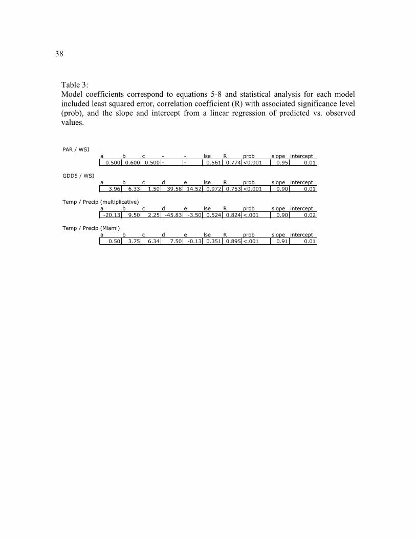
38 Table 3: Model coefficients correspond to equations 5-8 and statistical analysis for each model included least squared error, correlation coefficient (R) with associated significance level (prob), and the slope and intercept from a linear regression of predicted vs. observed values.

PAR / WSI

a b c - - lse R prob slope intercept

0.500 0.600 0.500 - - 0.561 0.774 <0.001 0.95 0.01

GDD5 / WSI

a b c d e lse R prob slope intercept

3.96 6.33 1.50 39.58 14.52 0.972 0.753 <0.001 0.90 0.01

Temp / Precip (multiplicative)


-20.13 9.50 2.25 -45.83 -3.50 0.524 0.824 <.001 0.90 0.02

Temp / Precip (Miami)


0.50 3.75 6.34 7.50 -0.13 0.351 0.895 <.001 0.91 0.01

39 Table 4: Global total NPP, uncertainty in global total NPP, maximum modeled NPP value, and percent agreement between modeled NPP and observations. Median

global NPP (Gt-C)

90% Confidence interval 5th %ile 95th%ile

Maximum modeled NPP (g-C m-2 yr-1)

Growing Season PAR – Water Stress Index

61.3 55.6 73.9 1577

Growing Degree Days – Water Stress Index

41.8 39.2 44.6 1559

Temperature – Precipitation (multiplicative)

52.0 47.3 54.7 1561

Temperature – Precipitation (Miami)

45.1 36.5 51.7 1164

40

Figure 1. Model-simulated (a) growing degree-days calculated as the annual sum of daily mean temperatures over a threshold of 5°C and (b) water stress index calculated as the ratio of actual evapotranspiration to potential evapotranspiration. Values closer to zero indicate an increased water stress.(c) Average photosynthetically active radiation(PAR) during the growing season. The growing season is defined as any day with an average temperature greater than zero. (d) Total annual precipitation and (e) average annual temperature from New et al. [2002].

41

Figure 2. Spatial distribution of NPP observations collected from the ORNL DAAC NPP database (http://www-eosdis.ornl.gov/NPP/npp_home.html) and other primary literature sources. See Table 1 for all data sources used.

42

Figure 3. NPP observations binned according to climate variables: (a) growing season PAR and a water stress index, (b) growing season PAR and a water stress index, and (c) annual precipitation and average annual temperature. The median value of NPP is displayed.

43

Figure 4. Net primary productivity as a function of (a) growing season PAR and water stress index, (b) growing degree-days (base 5) and water stress index, (c) annual average temperature and annual precipitation (multiplicative ), and (d) annual average temperature and annual precipitation (Miami). Global NPP for these models are 61.3 (55.6, 73.9) GtC, 41.8 (39.2, 44.6) GtC, 52.0 (47.3, 54.7) GtC, and 45.1 (36.5, 51.7) respectively. Values in parentheses bound the 90% confidence interval.

44

Figure 5. Histogram of NPP values binned by 200 units of NPP. There is a general trend of more area occupied by less productive land occupied by highly productive land.

Histogram of Global NPP

45

Figure 6. (a) Median and quartile observed NPP for each 2.5° latitude band that contained observed data (dashed lines) and comparison of modeled NPP in cells with observed data (solid lines) and (b) average modeled NPP over 2.5 latitude bands for all grid cells.

46

Figure 7. Average NPP over 14 biomes. Biomes defined by Ramankutty and Foley [1999]. (a) Models averaged only over cells with observations and (b) models averaged over all grid cells.

47

Chapter 3

Climatic and Edaphic Determinants of Aboveground Biomass Regrowth Rates in Tropical Forests

David P.M. Zaks Center for Sustainability and the Global Environment (SAGE) Nelson Institute for Environmental Studies University of Wisconsin 1710 University Avenue, Madison, WI 53726, USA

48 Abstract: The dynamics of tropical land-use / land cover change include deforestation, agricultural

use, land abandonment and forest regrowth. Across the tropics the rate at which forests

recover and sequester carbon is not fully understood. This study uses climate and soils

data at the pan-tropical scale to model rates of aboveground biomass regrowth in tropical

secondary forests. Data from primary literature studies across the tropics are used to fit

statistical models using biophysical variables, such as a forest climatic growth index and

soil pH. Results are shown as biomass accumulation in tropical forests annually. Policy

implications of re-growing forests are also discussed.

49 3.1 Introduction

Tropical forests are responsible for providing a vast array of ecosystem goods and

services such as food and fiber production, climate regulation, water purification, disease

regulation, flood control, and cultural services as well. There are also opportunities to

provide a broad suite of ecosystem services through management of re-growing forests

and the reforestation or afforestation of currently deforested or degraded lands. Re-

growing forests also deliver ecosystem goods and services, such as food and fiber, at a

local scale [Foley et al. 2007].

The delivery of ecosystem goods and services from tropical forests is being

threatened by land-use activities that are rapidly transforming tropical landscapes around

the world [Foley et al., 2005; Foley et al., 2007; Ramankutty et al., 2007]. Of particular

interest, tropical forests account for approximately 45% of global aboveground terrestrial

carbon storage, and are being threatened by increased rates of clearing [Watson et al.

2000]. Carbon is transferred from the biosphere to the atmosphere with the conversion

and degradation of forested land as vegetation is burned, or decays after clearing.

Deforestation and other land-use modifications are increasing in scale and pace

throughout the tropics, releasing carbon [Ramankutty et al., 2007]. Without chemical

inputs, poor soil fertility in many areas in the tropics leads to land abandonment and the

regrowth of natural vegetation. When land is abandoned, carbon accumulates in biomass

as the vegetation cover reverts back to forest.

While the scientific understanding of the dynamics of tropical forests has vastly

grown, there remain uncertainties. Reducing uncertainty in the biomass stocks in tropical

secondary forests is an important step in reducing the total uncertainty in carbon

50 emissions from tropical land-use change [Brown et al. 1995]. Further, the dynamics of

tropical forest clearing and subsequent land use are also large sources of uncertainty in

the global carbon balance [Ramankutty et al., 2007]. There is an ongoing debate in the

literature as to the rate and spatial distribution of tropical deforestation, and the associated

emission of carbon dioxide to the atmosphere [Achard et al. 2002; DeFries et al. 2002;

Houghton et al. 2000; McGuire et al. 2001; Ramankutty et al. 2007]. As some of the

deforested land reverts back to forest, it is important to know where this is occurring and

the rate of growth.

Initial projects have focused on determining the carbon balance of tropical forest

ecosystems [Lahsen and Nobre, 2007], but current methods (direct measurement and

remote sensing) have yet to produce accurate estimates of areas in re-growth across the

tropics, or their carbon content. Ground based studies are often hampered by the limited

information available about the history of forest plots. Previous chronosequence studies

only used early successional stands in which the ages of re-growing forests were known

[Johnson et al. 2000; Zarin et al. 2001; Zarin et al. 2005; Silver et al. 2000]. Assessing

age in tropical forests is more difficult than temperate forests due to lack of growing

season rings and incomplete land-use histories of disturbed areas. In most cases, scientists

who analyzed the study sites or local landholders provided the age assessments for

individual sites. The land-use history often is lost as farmers or other landholders move,

convert a parcel to a permanent land-use, or simply do not record the transitional

pathways of their land. While there is a large amount of land currently in some stage of

re-growth, the network of observations is limited by the paucity of available data.

51 The intensity of land-use before abandonment is thought to affect the rate at

which it re-grows [Gauriguata & Ostertag 2001; Chazdon 2000] It was once believed

[Brown and Lugo 1990; Richards 1955] that tropical secondary forests were suboptimal

in terms of species composition and wood quality, but further research has shown that in

most scenarios, as long as the seed bank is not totally diminished, such as after intensive

agriculture, secondary forests in the tropics can eventually become indistinguishable from

primary forests in terms of stored carbon and other ecosystem services delivered

[Gauriguata and Ostertag, 2001]. The intensity and duration of prior land-use has shown

to be a significant factor in both the regrowth rates and maximum aboveground biomass

reached, but insufficient data was available to test those correlations for this study.

The large spatial area of interest and the numerous studies reporting changes in

biomass stocks over time allows for an empirical methodology to be used to estimate

biomass re-growth rates. Over large scales, it has been shown that spatial patterns of net

primary productivity and biomass accumulation are related to climatic and edaphic

factors [Brown and Lugo 1990; Johnson et al. 2000; Zaks et al. 2007; Zarin et al. 2001,

Zarin et al. 2005, Zobler, 1986]. Johnson et al. [2000] presented methods to model

aboveground biomass re-growth using chronosequence data from both temperate and

tropical forests, and this approach was tested in Zarin et al. [2001, 2005] in the Amazon

region. The method uses the growing-season degree-year (GSDY) index as a proxy for

biomass. The index is based on the percentage of the year when monthly precipitation is

greater than 100mm (deemed the growing season), the average temperature during the

growing season and the age of the stand. A linear regression model was used for non-

sandy soils, where productivity is higher, and a log regression was used for sandy soils

52 where nutrient and water limitation restricts biomass accumulation. This approach is only

valid for young secondary forest stands, as the vigorous growth in the early successional

stages gives way to slower growth.

Studies have described the governing biotic and abiotic drivers of biomass re-

growth on global [Johnson et al. 2000] and basin scales [Zarin et al. 2001; Zarin et al.

2005], but no assessment has focused strictly on the pan-tropics. While global

assessments are inherently useful, focusing on a specific region or biome often reveals

system drivers that were not apparent in the larger scale study. The dynamic and complex

land use systems in the tropics cycle a large quantity of land through some state of

regrowth, storing carbon in biomass and in the soil [Fearnside 1996, Nepstad et al. 1991,

Cardille and Foley 2003, Hirsch et al. 2004, Ramankutty et al. 2007]. Tracking the fate

of the carbon through land-use transitions is imperative for both policy and carbon cycle

science questions [Gibbs et al., in prep].

3.2 Methods This study focuses on the rate of re-growth of tropical forests and their rates of

carbon accumulation. The statistical model presented here expands on previous studies

that illustrate how climatic and edaphic variables control patterns of aboveground

biomass regrowth [Johnson et al. 2000; Zarin et al. 2001; Zarin et al. 2005; O'Neill and

DeAngelis 1981]. Chronosequence data were summarized from peer-reviewed literature

at 61 geographically distinct sites throughout the tropics, for a total of 200 plots (Figure

1a). A histogram analysis of the data revealed that the largest age class of sample sites

was the newly cleared - 5 years (Figure 1b).

53 We attempted to find relationships between biomass regrowth and simple

biophysical variables, such as average temperature, precipitation and growing degree

days, but no significant relationships were found. The growing-season degree-year

approach (GSDY) or forest climatic growth index (FCGI), first proposed by O’Neill and

DeAngelis [1981], was used to simulate re-growth rates. FCGI is an index that

accumulates conditions favorable for forest growth – adequate rainfall and temperature

heat units. A sufficient amount of energy and water during the growing season are

required to drive photosynthesis reactions [Bonan 2002]. In previous implementations of

FCGI to model biomass accumulation, the fraction of sand in the soil (classified as either

"sandy" or "non-sandy") was used to differentiate between faster growing areas with

higher nutrient and water availability [Johnson et al. 2000; Zarin et al. 2001; Zarin et al.

2005]:

FCGI = A x G x T (1)

where A is the stand age, G is the percentage of the year that is in the growing season

(when monthly precipitation is greater than 100mm), and T is the average growing season

temperature (Figure 2a-c). Biomass (kg m-2) accounts for only the aboveground live

biomass. The Zarin et al. [2001] model was fit to biomass data for early successional

stands, and in this case it is appropriate to use a linear model. The original model was

global in scope, and temperature during the growing season was a more significant

portion of the model. The mean temperature at the observation sites during the growing

season was 25.4±1.1, indicating the low variability of tropical temperatures, and

highlighting the need for additional terms in the model.

54 This study takes advantage of the latest global biophysical data sets available, and

ground-based observed data. Observed monthly mean climate data were entered in the

model at 10' (1/6°) latitude x longitude spatial resolution [New et al. 2002] -- an

improvement over previous climate datasets. Mean monthly temperature and mean

monthly precipitation from the time period 1961 – 1990 were used to compute the

growing season (number of months where precipitation is greater than 100mm) and the

average temperature of those months.

Climate is an important factor in growth, but soil quality also plays a role in the

vigor of regrowth following disturbance. Many soils in tropical regions are old and

weathered, as they have not recently been refreshed by volcanic activity or other nutrient

deposition [Schlesinger, 1997]. The ISRIC-WISE global data set of derived soil

properties (5' latitude x 5' longitude spatial resolution) is a spatially extrapolated

representation of over 10,000 soil cores from around the world [Batjes, 2002]. It includes

data on several soil layers as well as many useful observed and derived soil

characteristics. For this study, useful parameters include organic carbon, total nitrogen,

cation exchange capacity, bulk density, available water capacity and pH.

Due to the coarseness of the ISRIC dataset, in many cases a single value was

assigned to an entire soil class, leading to little apparent variation among soils of the field

sites in this study. Other variables simply had insignificant correlation with biomass, or

were highly covariant with other variables. The characteristics for desirable model

variables were heterogeneity among observations, strong correlation to biomass and

biophysical rationality.

55 Most tropical forests are assumed to be phosphorus-limited [Chapin et al. 2002],

but no dataset of soil phosphorus is available for the pan-tropics. Soil Reaction or pH is a

useful measure of soil fertility [Juo and Franzluebbers, 2003] and is included in the

Batjes [2002] dataset. In tropical soils, pH has a strong influence over mobility of

aluminum, calcium and magnesium ions [Fearnside, 1998; Laurance 1999]. Acidic soils

are highly leached and contain reduced levels of mineral nutrients, like the already-

limiting phosphorus, and high concentrations of aluminum and calcium ions, while basic

soils contain large amounts of calcium carbonate [Juo and Franzluebbers, 2003; Laurance

et al. 1999]. Slightly acidic to neutral (5.3>pH<7.0) has been found to be the most

suitable soil condition for growth [Juo and Franzluebbers, 2003].

While many of the observations from the literature gave site-level descriptions of

the local climate and soil properties, we used the global datasets to maximize consistency

across sites. Each observed site was assigned the climate and soil data from the global

grids based on their longitude / latitude. The growing-season degree product ranged from

5.78 in Venezuela to 27.31 in Borneo. pH ranged from 4.7 in the eastern Amazon region

and in northern Africa to 6.8 southern Africa and in eastern Brazil in the dataset.

The biomass data were divided so that all sites with the optimal (5.3<pH<7.0)

were in one grouping, while the sub-optimal sites (pH<5.3) were in a second grouping.

Linear regressions of the optimal and sub-optimal biomass groups and the Forest

Climatic Growth Index (FCGI) were carried out. A t-test was then conducted to

determine the significant differences between the slopes of the regressions.

56 3.3 Results

In general, modeled values of biomass were highest in the humid tropics, where the

soil pH was within the optimal range of 5.3 to 7.0. The lowest values of biomass were in

areas occupied by dry tropical forests on poor soils. Accumulated biomass ranged from

0.12 t/ha to 7.92 t/ha per year, well within the published range of variability [Zarin et al.

2001; Zarin et al. 2005; Silver et al. 2000].

Differences were expected between the biomass re-growth rates for optimal and sub-

optimal pH soils. A t-test confirmed that biomass re-growth on soils with a pH in the

range of 5.3 to 7 was significantly faster than on poorer, more acidic soils. The regression

coefficients for the models ranged from .16 (pH>5.3; pH<7) to .27 (pH<5.3). These

values are relatively low, but were consistently higher than other model fits that were

attempted. Binning of the data to reduce variability was attempted, but the paucity of sites

prohibited this methodology.

The resulting model coefficients from the regression were then applied to the gridded

climate and soil data to obtain spatial representations of potential accumulation of

biomass at 10’ resolution in latitude by longitude (Figure 5). The model results are shown

as a yearly biomass increment after the disturbance event. As the model used is linear,

biomass accumulation can easily be calculated for any of the first 25 years of regrowth.

This model should not be used to calculate biomass after 25 years of regrowth as rates

have been shown to decrease after that, and are not well simulated by the linear form of

the model. Biomass accumulation after 25 years of growth is shown in figure 6, where

the maximum biomass accumulation is 198 tonnes/ha in Borneo.

57 The tropics are a geographically diverse region. The three dominant ecoregions

found in the tropics are (from most to least productive) tropical rainforest, tropical moist

forest and tropical dry forest. Similar to the FCGI, temperature and precipitation are used

to delineate ecoregions, although ecoregions are discrete and the FCGI is a continuous

measure. Summarizing regrowth rates by ecoregion (Table 1) shows more productive

ecosystems also have faster regrowth rates.

Rudel [2005] divided the tropics into seven regions based on climatic, geographic and

social parameters (Figure 8). The tropics are diverse across these spectra, and that is

reflected in their regrowth rates as well. Regions that contain large amounts of tropical

rainforest have higher average rates of growth, and regions comprised mostly of dry

forests and savannah has lower growth rates (Table 2). South America has the highest

rates of regrowth that averages 189.4 tons/ha, while East Africa has the lowest rate of

regrowth in the tropics with 49.3 tons/ha for the first 25 years.

Model results were sorted into 1º latitude bands and averages for each were

calculated (Figure 9). Zonal-average model results follow general latitudinal trends, with

regrowth rates increasing with proximity to the equator. The model results around 15º

are dominated by the Sahel region, which is mostly savannah / grassland and contains

relatively little biomass compared to other tropical biomes. Other regions in that latitude

band (Central America, Southern India, and the Southeast Asian complex) are generally

more productive, but contain less area.

As human pressure on tropical ecosystems increase, protected areas have emerged as

one avenue to offer a more sustainable path for development. Assessing which areas

contain the most biodiversity, carbon, water and cultural resources is needed to protect

58 the most valuable areas. Existing international, national and regional protected areas from

the World Conservation Union (IUCN) were used to summarize regrowth rates in current

protected areas within each of the seven tropical regions and compared to the baseline

rate for the entire region (Figure 10, Table 2). In most regions, the difference between

regrowth rates in currently protected areas and the entire region is negligible. In Central

America, regrowth rates are higher in protected areas than the baselines, while regrowth

rates in South America are lower in protected areas. As protected areas in tropical

countries expand, the criteria used to select these areas should consider biomass stocks as

well as regrowth rates in addition to biodiversity richness and species endemism.

Patterns of biomass accumulation can be compared to rates of net primary production

(NPP). The main components of NPP are leaves, stems, roots and fine roots, of which

stems and roots have long turnover times (~40 years) in tropical biomes opposed to

leaves and fine roots (~1 year). According to Kucharik et al. [2000] and Barford [in

prep.] 30% of NPP is allocated to stems, while 10% is allocated to roots. Using the

modeled NPP dataset from Zaks et al. [2007], annual biomass accumulation can be

calculated (Figure 11a). Differencing the datasets reveals that in most equatorial areas,

the uptake rates of the biomass model were greater than the NPP model and in areas

further from the equator, NPP values were generally greater than biomass uptake rates

(Figure 11b).

3.4 Discussion Vegetation growth is controlled by multiple biotic and abiotic factors. In addition

to temperature, precipitation and soils, which have been accounted for in this analysis,

59 there are other variables that govern the differences in biomass densities from plot to

regional scales including climate and land-use. The low coefficients of determination of

the regressions (0.29 and 0.23) might be explained by variables not included in this study,

but which have significant control over re-growth. It is important to note that this

modeling framework is not designed to account for trends in climate, as the data used was

averaged over a thirty-year period, nor is it designed to simulate inter-annual variability,

or biomass response to climatic variations such as El Niño or La Niña.

Large-scale models often have the drawback of averaging small-scale changes

that might be caused by topography, microclimate or diverse management practices. As

the areas of re-growth included in this study were primarily from anthropogenic

disturbances, and not from natural disturbances such as wind-throw or fire, discussion of

the impacts of land-use on forest re-growth is warranted. While climate, soil, and stand

age were accounted for in this model, disturbance duration and intensity were not

included, due mostly to the paucity of data. Previous studies [Steininger, 2000; Silver et

al., 2000, Zarin et al. 2005] showed differences in re-growth rates depending on past

land-use history, although Zarin et al. [2001] showed no significant difference. In most

cases, with increasing intensity and duration of the disturbance, both rate of biomass

accumulation and maximum potential biomass are likely to decrease [Silver et al. 2000].

Less than half of the field observations collected for this study denoted either the

intensity or duration of the disturbance; therefore, it could not be included in the model.

There is also a discrepancy between the scale of the model simulations and the

field observations of biomass. The size of a 10’ grid cell at the equator is 345 km2, while

the average size of a field study area is often several hectares or less. Local observations

60 of biomass are influenced by landscape heterogeneity, including changes in microclimate

and soil fertility due to land-use, historical patterns of disturbance, species composition,

altitudinal gradients, and hydrology.

In prior studies, differentiating soil texture, as shown in Johnson et al. [2000] was

limited to the available soil characteristics in Zobler [1986]. New global scale gridded

soil databases [Batjes 2002] map many more soil properties that might have stronger

correlations to aboveground biomass regrowth rates. While this model categorized

biomass data by pH, future iterations of the model can include other complementary soil

variables such as available water capacity, nitrogen, organic carbon and bulk density. As

phosphorus is one of the key limiting nutrient for most tropical systems, it would be of

great value to have a global soil phosphorus dataset. Also, the Zobler [1986] data set only

represents the dominant soil type in the first 30cm of depth, but Batjes [2002] contains

data for soils at 30cm depth, and the subsoil down to 100cm for the top 10 dominant soil

classes in each grid cell.

Another caveat in the data set is that most biomass data reported in the primary

literature are derived from allometric equations that relate the diameter at breast height

(DBH) of sampled trees to their mass (or dry mass) after destructive harvest. Some

equations also include the height of the tree in the calculation. In some studies, equations

are produced based on an individual stand, while other equations are syntheses of an

entire region. Studies [e.g. Baker et al. 2004] have illustrated that some sample plots in

the tropics are preferentially chosen for their large trees, skewing the resulting equations,

and biomass distributions. The field methodology might also play a role in introducing

error into biomass estimates. Standard practice is to take a diameter measurement of the

61 tree at breast height (1.37m) but many tropical trees have buttresses that could skew the

resultant equation [Clark 2002]. Furthermore, Baker et al. [2004] illustrated the

importance of wood density (and hence carbon content) when using allometric equations.

Brown [2002] stress the importance of using a proper equation for the geographic area

and succession stage that is being studied as opposed to more general equations. Other

studies report biomass using allometric equations developed in different regions, which

may not be applicable. While allometric equations are currently the most feasible way to

report plot-level biomass, the error introduced by this method needs to be assessed.

Each step of the analysis includes some error, as the precision of the datasets,

measurements and models are not fully known. In the input soils and climate data, the

error is left unquantified, making it difficult to assess the total error for the model output.

Error is also unquantified in the observations. While it would be difficult not to include

some error term in the results, the scarcity of data prevents a large-scale error analysis.

Following the methods of Zaks et al. [2007], error terms were computed for a global

scale empirical model by binning the data, and determining the distribution of observed

data for observations with similar climates. While this method was attempted, there was

much less data than the previous analysis, not yielding enough data for a complete

analysis.

3.5 Conclusions Tropical forests are globally important for many reasons, including their functions

of climate regulation, reliable provision of freshwater, and maintenance of biodiversity

habitat. While the rates and patterns of deforestation are becoming better constrained, the

62 fate of the cleared land is still highly uncertain. It is estimated that ~40% of tropical

forests are in some stage of regrowth following deforestation, logging, and cycles of

shifting cultivation [Brown and Lugo, 1984]. The tropics are a diverse region, but a

sufficient amount of data has been collected from spatially and climatically distinct areas

to enable models to be constructed, and then applied over the pan-tropical area.

At a pan-tropical scale, the basic ecological functions that control many of these

systems are still poorly constrained. This body of work is an important part in reducing

the uncertainty of carbon emissions from tropical deforestation and subsequent patterns

of land-use [Gibbs, In Prep; Ramankutty et al. 2007]. Work is ongoing to strengthen our

understanding of the patterns of deforestation around the tropics, their proximate and

ultimate drivers, and the fate of the cleared land.

The model presented here will be incorporated into a next-generation biosphere

model, Predicting Ecosystem Goods and Services for Understanding Sustainability

(PEGASUS), currently under development at the Center for Sustainability and Global

Environment, that will bring together research components on the distribution of

ecosystem goods and services, dynamic patterns of land-use following deforestation, the

spatial extent of deforestation, biomass contained in mature forests and biomass in re-

growing forests [Barford, in prep]. The resulting simulations of this model will simulate

the fluxes of carbon between the biosphere and atmosphere and the implications for

climate, people and ecosystems.

Future policies will demand a better understanding of how tropical forest systems

function, especially at their ever-broadening interface with people. As illustrated here,

using field data and models together can characterize broad scale ecological patterns and

63 thus strengthen our understanding of these complex systems. More field data, especially

from previously poorly sampled regions, are needed to strengthen our concept of the

relationships between climate, soil, and biomass regrowth.

64

Acknowledgements: I would like to thank N. Ramankutty, J.A. Foley, H.K. Gibbs, and C.C. Barford for their assistance with this project. This work was supported by NASA Terrestrial Ecology grant (NAG5-13351).

65 References: Achard, F., et al. (2002), Determination of deforestation rates of the world's humid tropical forests, Science, 297, 999-1002.

Baker, T. R., et al. (2004), Variation in wood density determines spatial patterns in Amazonian forest biomass, Global Change Biology, 10, 545-562.

Barford, C. C. (in prep.), PEGASUS: Predicting Ecosystem Goods and Services for Understanding Sustainability.

Batjes, N. H. (2002), Revised soil parameter estimates for the soil types of the world, Soil Use and Management, 18, 232-235.

Bonan, G. B. (2002), Ecological climatology: concepts and applications, xi, 678 p. pp., Cambridge University Press, New York.

Brown, I. F., et al. (1995), Uncertainty In The Biomass Of Amazonian Forests - An Example From Rondonia, Brazil, For. Ecol. Manage., 75, 175-189.

Brown, S. (2002), Measuring carbon in forests: current status and future challenges, Environmental Pollution, 116, 363-372.

Brown, S., and A. E. Lugo (1984), Biomass Of Tropical Forests - A New Estimate Based On Forest Volumes, Science, 223, 1290-1293.

Brown, S., and A. E. Lugo (1990), Tropical Secondary Forests, Journal Of Tropical Ecology, 6, 1-32.

Cardille, J. A., and J. A. Foley (2003), Agricultural land-use change in Brazilian Amazonia between 1980 and 1995: Evidence from integrated satellite and census data, Remote Sensing of Environment, 87, 551-562.

Chapin, F. S., et al. (2002), Principles of terrestrial ecosystem ecology, xiv, 436 p. pp., Springer, New York.

Chazdon, R. L. (2003), Tropical forest recovery: legacies of human impact and natural disturbances, Perspectives In Plant Ecology Evolution And Systematics, 6, 51-71.

Clark, D. A. (2002), Are tropical forests an important carbon sink? Reanalysis of the long-term plot data, Ecol. Appl., 12, 3-7.

Defries, R. S., et al. (2002), Carbon emissions from tropical deforestation and regrowth based on satellite observations for the 1980s and 1990s, Proceedings of the National Academy of Sciences of the United States of America, 99, 14256-14261.

Fearnside, P. M. (1996), Amazonian deforestation and global warming: Carbon stocks in

66 vegetation replacing Brazil's Amazon forest, For. Ecol. Manage., 80, 21-34.

Fearnside, P. M., and R. I. Barbosa (1998), Soil carbon changes from conversion of forest to pasture in Brazilian Amazonia, For. Ecol. Manage., 108, 147-166.

Foley, J. A., et al. (2007), Amazonia revealed: forest degradation and loss of ecosystem goods and services in the Amazon Basin, Frontiers In Ecology And The Environment, 5, 25-32.

Foley, J. A., et al. (2005), Global consequences of land use, Science, 309, 570-574.

Gauriguata, M. R., and R. Ostertag (2001), Neotropical secondary forest succession: changes in structural and functional characteristics, For. Ecol. Manage., 148, 185-206.

Gibbs, H. K. (in prep.), Can Forest Carbon Stocks In Developing Countries Be Measured?

Hirsch, A. I., et al. (2004), The net carbon flux due to deforestation and forest re-growth in the Brazilian Amazon: analysis using a process-based model, Global Change Biology, 10, 908-924.

Houghton, R. A., et al. (2000), Annual fluxes or carbon from deforestation and regrowth in the Brazilian Amazon, Nature, 403, 301-304.

Johnson, C. M., et al. (2000), Post-disturbance aboveground biomass accumulation in global secondary forests, Ecology, 81, 1395-1401.

Juo, A. S. R., and K. Franzluebbers (2003), Tropical soils: properties and management for sustainable agriculture, ix, 281 p. pp., Oxford University Press, New York.

Kucharik, C. J., et al. (2000), Testing the performance of a Dynamic Global Ecosystem Model: Water balance, carbon balance, and vegetation structure, Global Biogeochemical Cycles, 14, 795-825.

Lahsen, M., and C. A. Nobre (2007), Challenges of connecting international science and local level sustainability efforts: the case of the Large-Scale Biosphere-Atmosphere Experiment in Amazonia, Environmental Science & Policy, 10, 62-74.

Laurance, W. F. (1999), Reflections on the tropical deforestation crisis, Biol. Conserv., 91, 109-117.

Mcguire, a. D., et al. (2001), Carbon balance of the terrestrial biosphere in the twentieth century: Analyses of CO2, climate and land use effects with four process-based ecosystem models, Global Biogeochemical Cycles, 15, 183-206.

Nepstad, D. C., et al. (1991), Recuperation Of A Degraded Amazonian Landscape - Forest Recovery And Agricultural Restoration, Ambio, 20, 248-255.

New, M., et al. (2002), A high-resolution data set of surface climate over global land areas, Clim. Res., 21, 1-25.

67 O’Neill, R., and D. DeAngelis (1981), Comparative productivity and biomass relations of forest ecosystems, in Dynamic Properties of Forest Ecosystems, edited by R. RF, Cambridge.

Ramankutty, N., et al. (2007), Challenges to estimating carbon emissions from tropical deforestation, Global Change Biology, 13, 51-66.

Richards, P. (1955), The Secondary Succession in the Tropical Rain Forest, Science Progress London, 45-57. Rudel, T. K., et al. (2005), Forest transitions: towards a global understanding of land use change, Global Environmental Change-Human and Policy Dimensions, 15, 23-31.

Schlesinger, W. H. (1997), Biogeochemistry: an analysis of global change, 2nd ed., xiii, 588 p. pp., Academic Press, San Diego, Calif.

Silver, W. L., et al. (2004), Carbon sequestration and plant community dynamics following reforestation of tropical pasture, Ecol. Appl., 14, 1115-1127.

Steininger, M. K. (2000), Secondary forest structure and biomass following short and extended land-use in central and southern Amazonia, Journal of Tropical Ecology, 16, 689-708.

Watson, R. T., and Intergovernmental Panel on Climate Change. (2000), Land use, land-use change, and forestry, 377 p. pp., Published for the Intergovernmental Panel on Climate Change [by] Cambridge University Press, Cambridge, UK; New York.

Zaks, D. P. M., et al. (2007), From Miami to Madison: Investigating the relationship between climate and terrestrial net primary production, Global Biogeochemical Cycles, 21, -.

Zarin, D. J., et al. (2005), Legacy of fire slows carbon accumulation in Amazonian forest regrowth, Frontiers In Ecology And The Environment, 3, 365-369.

Zarin, D. J., et al. (2001), Potential biomass accumulation in Amazonian regrowth forests, Ecosystems, 4, 658-668.

Zobler, L. (1986), A world soil file for global climate modeling, NASA technical memo no. 87802, 33 p.

68

Table 1: Average biomass in the three tropical ecoregions on an annual basis.

Ecoregion Average Biomass (Tonnes Biomass / year) Tropical dry forest 2.28 Tropical moist deciduous forest 3.07 Tropical rainforest 4.30

69 Table 2: Comparison of regrowth rates for tropical regions and the protected areas

within them.

Average biomass regrowth (tonnes/ha) per year in entire region

Average biomass regrowth (tonnes/ha) per year in protected areas

Southeast Asia 4.83 4.80

West Africa 3.14 3.26

South Asia 2.27 2.71

South America 7.58 4.08

East Africa 1.97 1.80

Central America 3.22 3.94

Central Africa 3.20 3.06

70 Figure 1a:

Figure 1b:

(1a) Spatial distribution of NPP observations collected from the primary literature(Johnson et al. 2000; Zarin et al. 2001; Zarin et al. 2005; Silver et al. 2000; Clark et al. 2001). (1b) Distribution of sample sites across age classes show that a majority of the sample sites are in the younger age classes.

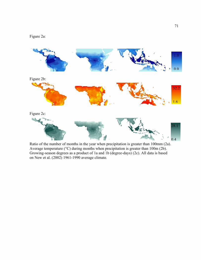
71 Figure 2a:

Figure 2b:

Figure 2c:

Ratio of the number of months in the year when precipitation is greater than 100mm (2a). Average temperature (°C) during months when precipitation is greater than 100m (2b). Growing-season degrees as a product of 1a and 1b (degree-days) (2c). All data is based on New et al. (2002) 1961-1990 average climate.

1.0 0.0

32.2 1.6

28.1 0.4

72 Figure 3:

Soil pH derived from ISRIC soil database [Batjes, 2002].

73 Figure 4:

Linear model of FCGI vs. Biomass. Data observations separated based on soil pH. Fertile soil pH >5.3 and less than, less fertile soils have pH < 5.3.

74 Figure 5:

Spatially explicit estimates of biomass regrowth per year. Maximum-modeled biomass uptake is 7.95 tonnes / ha / yr.

75 Figure 6:

Spatially explicit estimates of biomass regrowth over a 25 year period. Maximum-modeled biomass regrowth is 198 tonnes / ha and the minimum is 2.2 tonnes/ha.

76 Figure 7:

Major ecoregions of the tropics ranked from highest to lowest rates of biomass accumulation: rainforest, moist forest, dry forest.

77 Figure 8:

Regions of the tropics defined by Rudel (2005). Averaged over each region, South America has the highest biomass uptake rate, while East Africa has the lowest.

78 Figure 9:

Latitudinal distribution of biomass regrowth in the tropics. Rates of uptake peak around the equator in regions of high productivity and decrease towards the mid latitudes where productivity declines. Averaged over all three equatorial zones, the maximum rate of uptake is 4.3 tonnes/ha-1/yr-1.

Latitudinal Distribution of Annual Biomass Regrowth Rates

79 Figure 10:

Distribution of protected areas in the tropics. (Source: IUCN Protected Areas Database)

80 Figure 11a

Figure 11b

The results of biomass uptake rates from this study were compared to a global study of net primary productivity (Figure 11a) (Zaks et al. 2007). Net primary productivity values were converted to biomass uptake rates using published allocation data. Comparison of the two datasets was done using differencing (Figure 11b).

81

Chapter 4

Conclusion

The problem of global environmental change successfully captured attention in

both public and political spheres in the 21st century. Scientists are increasingly accepting

global warming as an anthropogenic phenomenon, and society is starting to assume

responsibility for its contributions to climate change. At the same time, our scientific

understandings of the effects of human land-use decisions on critical ecosystem goods

and services are increasing rapidly. With this public acceptance and simultaneous growth

in knowledge come important opportunities to enact policies to slow and hopefully repair

the damage that has been caused to the Earth system.

Policies and scientific research on the stocks and flows of carbon are now a

significant focus of international attention. From policy initiatives like the Kyoto Protocol

and Regional Greenhouse Gas Initiative to basin-wide scientific campaigns including the

Large-Scale Biosphere Atmosphere Experiment in Amazonia, decision makers and the

scientific community are amassing resources to better understand and ultimately reduce

humans’ impacts on the environment. While 75% of carbon emissions are from fossil

fuels, the remainder is from land-use change, and this issue is increasingly becoming a

focus in the next generation of climate policies [Houghton, 1995]. Two important

measures of carbon flux in terrestrial ecosystems are net primary productivity (NPP) and

biomass accumulation rates. Measuring, mapping and monitoring these fluxes of carbon

82 on a global scale are an important scientific contribution, but are currently in a nascent

stage of development.

Empirical studies are useful in detecting changes over a long time horizon, at fine

resolutions, across the globe. They can be incorporated into numerical models and used

in training remote sensing algorithms. The integration of place-based field data and

empirical models was the backbone to both studies presented here. Global scale empirical

studies would not be possible without the tireless work of researchers, some who dedicate

their entire careers, to measuring changes in research sites around the world. Through the

collaboration of researchers and the integration of their datasets at multiple scales,

bridges of ecological knowledge are being built between the local and global scales.

Human impacts on forest ecosystems can be observed at many scales and

considering the direct impact on these systems – moving beyond just considerations of

the carbon cycle – is also crucial. The human appropriation of net primary production

(HANPP) is one measure of the extent that the human species has usurped the resources

of earth. [Vitousek et al. 1986; Haberl et al. 2002; Imhoff et al. 2004; Foley et al. 2007].

Recent estimates show that 23.8% of global productivity is co-opted for human use

[Haberl et al. 2007]. In most areas the background NPP has decreased from activities

ranging from agriculture to urban expansion. Although in some areas the current NPP

rates are higher than background NPP due to intensive fertilization, irrigation and

mechanization of agriculture. HANPP research leverages agricultural and forestry

production statistics and simulations from dynamic global vegetation models to

illuminate previously unknown patterns and trends. The importance of these studies lies

83 in reframing what were prior seemingly benign numbers into a story that more effectively

portrays our collective actions on the planet.

Previous studies on HANPP require two main types of data: first, information on

global primary productivity and second, human uses of productivity such as agriculture,

forestry and pasture. Earlier studies calculated HANPP based on global totals of these

data, but new spatially explicit data gives added value to the HANPP concept. The results

of chapter two can be used as an input for spatially explicit calculation of HANPP. Foley

et al. [2007] recently used this dataset to illustrate differences in productivity between

managed and natural lands.

Studies of NPP, as presented in this thesis, help to reveal patterns of productivity

in new ways when joined with other data sets, such as in a HANPP analysis. The human

relationship to land-use change can be studied at a global scale, but the patterns and

processes (abiotic and human) of local and regional transformations drive the change

seen on the global scale. Across the tropics, patterns and pathways of land-use, such as

shifting agriculture, have converted large areas to a matrix of agriculture and regrowing

forests.

An increasing amount of land in the tropics is turning towards human uses in

ways that are significantly worrisome in terms of their carbon emissions and degradation

of other ecosystem services. Agriculture, predatory forestry, and livestock operations

expand into formerly forested areas to meet the needs of growing populations and

provide additional sources of income. Tropical forests and grasslands harboring an

immense amount of carbon and biodiversity can be detrimentally affected with

agricultural expansion. Tropical forests and savannahs not only contain 40% of the

84 global terrestrial carbon [Watson et al. 2001], but also are an important provider of

ecosystem goods and services [Foley et al. 2007]. When forests and savannahs are

converted to other uses, much of the carbon and nutrients stored in the biomass are lost

when the converted area is burned.

Tropical terrestrial ecosystems store many of their nutrients in plant biomass,

therefore the soil in most areas is nutrient deficient, and cannot provide sustained growth

to agriculture and are often abandoned after several years. It is estimated that in some

areas 30-50% of previously cleared land is in some state of regrowth [Fearnside 1996;

Houghton et al. 2000; Zarin et al. 2001]. These regrowing forests store carbon and

provide other ecosystem services and income sources for the local populations. There are

currently few incentives to rehabilitate degraded land, but the changing political

landscape may provide future motivations. In most cases, it is more profitable for a

landowner to deforest their land than to maintain the forest cover and associated

ecosystem services. Similarly, on currently degraded lands, few incentives are in place to

rehabilitate the land to sequester carbon. As identified in Chapter 3, soils and climate play

a role in determining the ability of a previously cleared land to sequester carbon in

biomass.

Findings from these studies can be combined with biodiversity, social and other

ecosystem service hotspot indicators to create a prioritized ranking of restoration

locations. One policy suggestion stemming from this research is devising an economic

policy whereby local stakeholders can be compensated for increasing rates of carbon

sequestration above a determined baseline through approved methods. The benefits of

providing incentives for people in these regrowing forests, beyond carbon sequestration,

85 are that re-growing forests provide other ecosystem goods and services that would also

likely increase, including water quantity and quality, and improved air quality from

reduced forest burning. For example, in Costa Rica, farmers are not only paid for carbon

sequestration, but also for maintaining water flows, preventing erosion, and reducing

flooding [Pagiola et al. 2005]. While it is outside the scope of the scientific community

to attach a value to changes in ecosystem services, it is important to provide the necessary

data on the biophysical changes and trade-offs among different services.

Whether calculating the human impact on the Earth using these newly presented

NPP data or highlighting areas of conservation in the tropics with high rates of growth,

societal decisions about what actions to take are not the responsibility of the scientists,

but of the public. Integrating this knowledge into adaptive management and governance

structures allows for constant feedback between information and action.

86

References Fearnside, P. M., and W. M. Guimaraes (1996), Carbon uptake by secondary forests in Brazilian Amazonia, For. Ecol. Manage., 80, 35-46. Foley, J. A., et al. (2007a), Amazonia revealed: forest degradation and loss of ecosystem goods and services in the Amazon Basin, Frontiers In Ecology And The Environment, 5, 25-32. Foley, J. A., et al. (2007b), Our share of the planetary pie, Proceedings of the National Academy of Sciences of the United States of America, 104, 12585-12586. Haberl, H., et al. (2007), Quantifying and mapping the human appropriation of net primary production in earth's terrestrial ecosystems, Proceedings of the National Academy of Sciences of the United States of America, 104, 12942-12945. Haberl, H., et al. (2002), Human appropriation of net primary production, Science, 296, 1968-1969. Houghton, R. a. (1995), Land-Use Change and the Carbon-Cycle, Global Change Biology, 1, 275-287. Houghton, R. A., et al. (2000), Annual fluxes or carbon from deforestation and regrowth in the Brazilian Amazon, Nature, 403, 301-304. Imhoff, M. L., et al. (2004), Global patterns in human consumption of net primary production, Nature, 429, 870-873. Pagiola, S., et al. (2005), Paying for Biodiversity conservation services - Experience in Colombia, Costa Rica, and Nicaragua, Mountain Research and Development, 25, 206-211. Vitousek, P. M., et al. (1986), Human Appropriation Of The Products Of Photosynthesis, Bioscience, 36, 368-373. Watson, R. T., and Intergovernmental Panel on Climate Change. (2000), Land use, land-use change, and forestry, 377 p. pp., Published for the Intergovernmental Panel on Climate Change [by] Cambridge University Press, Cambridge, UK; New York. Zarin, D. J., et al. (2001), Potential biomass accumulation in Amazonian regrowth forests, Ecosystems, 4, 658-668.

global patterns of ecological productivity and … patterns of ecological productivity and tropical...

Documents