lable at ScienceDirect

Journal of Environmental Management 90 (2009) 1178–1183

Contents lists avai

Journal of Environmental Management

journal homepage: www.elsevier .com/locate/ jenvman

Global warming and environmental production efficiency rankingof the Kyoto Protocol nations

Ehsan H. Feroz a,*, Raymond L. Raab b, Gerald T. Ulleberg c, Kamal Alsharif d

a Milgard School of Business, University of Washington, 1900 Commerce Street, Box 358420, Tacoma, WA 98402-3100, (253) 692-4728, USAb School of Business and Economics, University of Minnesota Duluth, 412 Library Drive, Duluth, MN 55812-2496 (218) 726-8508, USAc Department of Economics, University of Minnesota Duluth, Duluth, MN 55812, USAd Environmental Science and Policy Program, Geography Department, University of South Florida, 4202 E. Fowler Avenue, Tampa FL 33620, (813) 974-2739, USA

a r t i c l e i n f o

Article history:Received 9 January 2007Received in revised form 3 May 2008Accepted 15 May 2008Available online 2 July 2008

Keywords:UNO Kyoto ProtocolEnvironmental productionefficiency rankingGDPDEAGlobal warming

* Corresponding author. Tel.: þ1 253 692 4728.E-mail addresses: ehf2@u.washington.edu (E.H

(R.L. Raab), ulle0005@d.umn.edu (G.T. Ulleberg), alsh

0301-4797/$ – see front matter � 2008 Elsevier Ltd.doi:10.1016/j.jenvman.2008.05.006

a b s t r a c t

This paper analyzes the United Nations Organization’s Kyoto Protocol nations to address two questions.First, what are the environmental production efficiency rankings of these nations? Second, is therea relationship between a nation’s ratification status and its environmental production efficiency ranking?Our findings suggest that the nations that have ratified the Kyoto Protocol are more likely to beenvironmentally production efficient as compared to the nations that have not ratified the Protocol.

� 2008 Elsevier Ltd. All rights reserved.

1. Introduction

Ratifying the United Nations Organization’s (UNO hereafter)Kyoto Protocol is one of the most contentious policy initiatives onglobal warming and environmental issues. While many of the sig-natories to the Protocol, particularly developing and Europeannations (i.e., national governments or NGs hereafter) have generallyratified the treaty, there are just as many other NGs including mostprominently the United States, Australia, and the People’s Republicof China (PRC hereafter) that are yet to ratify the treaty. Althoughthere have been several attempts to reconcile the differencesbetween the NGs who have ratified the Protocol and those who areyet to ratify, it appears that the differences between the two blocksof NGs may be irreconcilable and based on rather strong domesticpolitico-economic considerations notwithstanding the seasonalelectoral political rhetoric on global warming issues as highlightedby recent press coverage in the United States and other parts of theworld.

We study the Kyoto Protocol NGs to address two specific issues:First, what are the environmental production efficiency rankings of

. Feroz), rraab1@d.umn.edu0018@umn.edu (K. Alsharif).

All rights reserved.

these NGs? Second, is there a relationship between an NG’s ratifi-cation status and its environmental production efficiency ranking?We use the data envelopment analysis (DEA) to compare the rela-tive performance of the signatory NGs since it is much moremeaningful to compare these NGs to each other’s efficiency recordas a relative benchmark in a truly global sense. We providedescriptive statistical evidence to establish a relationship betweenthe ratification status and environmental production efficiencyrank.

The rest of the paper is as follows. Section 2 provides a ratio-nale for the DEA model with details on the selection of individualinputs and outputs. Section 3 analyzes the environmental pro-duction efficiency status of the Kyoto Protocol NGs. Section 4examines the relationships between the environmental pro-duction efficiency ranks and ratification status. Section 5 con-cludes the paper.

2. Environmental production efficiency: a DEA approach

Of the various extant DEA models, the additive model employsa criterion of maximizing an NG’s material well-being (GDP) andhealth outcomes, while simultaneously minimizing pollutants thatinhibit the health and material well-being of the signatories. Themost efficient NG produces a maximum of material well-being and

2 The additive model primal below only dichotomizes the NGs as efficient (i.e., onthe frontier) or inefficient (i.e., below the frontier):

� �

E.H. Feroz et al. / Journal of Environmental Management 90 (2009) 1178–1183 1179

good health by utilizing technologies that result in a minimumrelease of hazardous compounds that cause environmental degra-dation. This logic allows for an environmental evaluation to showthat use of the least hazardous technologies in an NG’s agriculturaland industrial sectors may well result in lower pollution levels,more material well-being and better health outcomes. An‘environmentally production efficient’ NG produces the maximumnational output and ‘good health’ while emitting the minimum ofharmful effluents. Our model incorporates commonly discussedinterrelated environmental and economic components and sys-tematically incorporates them into an operational definition ofenvironmental production efficiency. The model is specified asfollows:

max : Y1 ¼ GDP per capitaY2 ¼ healthy average male life expectancy beyond sixtymin : X1 ¼ fertilizer use ð100g=hectare of arable landÞX2 ¼ pesticide use ðkg=hectare of croplandÞX3 ¼ commercial energy use ðkg of oil equivalent per capitaÞX4 ¼ CO2emissions ðmetric tons per capitaÞ

(1)

Units of Inputs and outputs:fertilizer use in 100 grams per hectare of arable land,commercial energy use in kilograms of oil equivalent per capita,carbon dioxide emissions in metric tons per capita,pesticide use in kilograms per hectare of cropland,healthy average life expectancy in years of males at age 60,per capita gross domestic product in 1995 US dollars 1

Specifically the additive DEA model simultaneously maximizesper capita GDP and male life expectancy and minimizes pollutants.This approach selects the particular set of weights or coefficients formaterial and health outcomes and pollution releases that allowa particular NG to achieve its highest production efficiency ranking.One linear program is computed for each NG and this proceduredetermines the unique best transformation relationship meetingthe optimization criterion. For a particular NG the importanceweights are chosen where the difference between the highestoutput and lowest input is the largest. The remaining NGs areconstrained to employ that NG’s ‘‘best practice’’ set of weights (seeRaab and Feroz, 2007 for technical details). This approach identifiesthose NGs that make the most efficient use of highly toxiccompounds.

Unlike the Charnes et al. (1981) or CCR model or the Bankeret al. (1984) or BCC model, the additive model is neither inputoriented nor output oriented only. CCR and BCC measure radialinefficiency by either input or output distance measures to thefrontier. Since the additive model is neither input nor outputoriented, DEA can construct an index that simultaneously maxi-mizes ‘‘good’’ indicators and minimizes ‘‘bad’’ indicators, evenwithout presuming a production or transformation relationship.Although our model does specify a loose production function, it isprimarily an environmental performance index. A brief account ofthe additive DEA model and the sensitivity analysis employed torank the NGs follows.

1 Data sources:

World Development Indicators (2001), World Bank: GDP, fertilizer use, com-mercial energy use, and CO2 emissions data.World Economic Forum, Yale Center for Environmental Law and Policy, andCIESIN, 2002 Environmental Sustainability Index: pesticide data.Table 4, Annex, 2002 Annual Report, World Health Organization: healthy aver-age life expectancy (HALE) data.

3. The additive DEA model and stability index formulationof efficiency indexes

As a linear programming application of technical efficiency, DEAconstructs an efficient frontier composed of those NGs thatconsume as little toxic compounds (inputs) as possible, whileproducing as much material and physical well-being (outputs) aspossible. Those NGs that comprise the efficient frontier are effi-cient, while those NGs not on the efficient frontier are inefficient(i.e., enveloped or dominated by the efficient NGs).

The additive model of Charnes et al. (1985) utilizes the convexhull of input consumption and output production for all the 36 NGsfor which complete data was available. These 36 NGs form theproduction possibility set (PE):

PE ¼(�

YT;XT�¼X36

i¼1

mi

�YT

i ;XTi

�;X36

i¼1

mi ¼ 1; mi � 0

)(2)

where i represents the general index of 36 NGs and (YjT, Xj

T) is thetransposed vector of outputs and inputs for a particular NG underevaluation, denoted as NGi. The pollution efficiency status (efficientor inefficient) for each NG is determined by comparing its inputsand outputs to PE. If no other NG’s components, observed orhypothetical, in PE consume the same or less input while simul-taneously producing more or the same output, with at least onestrict inequality, then NGi is deemed technically efficient. ThoseNGs not meeting the above criteria are deemed pollution inefficientrelative to the benchmark and are enveloped or dominated by thefrontier. This form of the additive model yields only a classificationof pollution efficient and inefficient NGs, but does not yield a rankordering of NGs from most robustly efficient to most robustlyinefficient.2

Cooper et al. (2001) and Cooper et al. (2007) developeda sensitivity technique for the additive DEA model. It definesthe necessary simultaneous perturbations of a given NG tocause it to move to a condition of ‘‘virtual’’ efficiency. Virtualefficiency is defined as a point of the efficient frontier whereany minuscule detrimental perturbation (increase in inputs and/or decrease in outputs) will cause an efficient NG to becomeinefficient or any minuscule favorable perturbation (decrease ininputs and/or increase in outputs) will cause an inefficient NGto become efficient. The stability index defines the minimumsimultaneous perturbations to the input–output vector foreach NG to alter its efficiency classification. A single linearprogram is computed for each NG in the efficient group andanother single linear program is computed for each NG in theinefficient group (see Alsharif et al., 2008 for the details of thisapproach).

min � eTD�1sY

sþ þ �eTD�1sX

s� ;

s:t: Yl � sþ ¼ YjXl þ s� ¼ Xj

eTl ¼ 1l; sþ; s� � 0

(5)

where Y and X are the matrices of the outputs and inputs, and sþ and s� are theshortfall in production and excess consumption slacks. The eT is the summationvector. As the additive model is not units invariant, we would note that Y and X aretransformed by component standard deviations in the objective function D�1

sYand

D�1sX

to assure common results regardless of the units of measure chosen for eachcomponent. [see Raab and Feroz (2007) for an explanation and a relatedapplication].

E.H. Feroz et al. / Journal of Environmental Management 90 (2009) 1178–11831180

4. DEA application to the Kyoto treaty nations

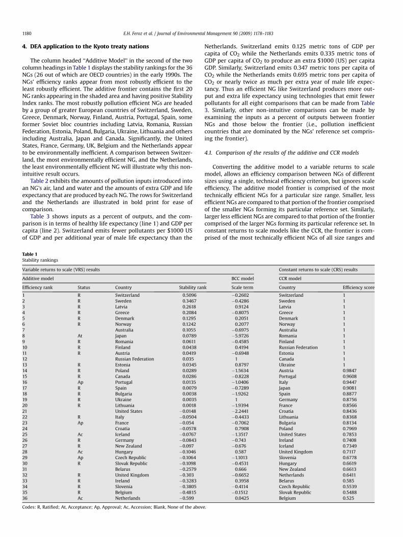
The column headed ‘‘Additive Model’’ in the second of the twocolumn headings in Table 1 displays the stability rankings for the 36NGs (26 out of which are OECD countries) in the early 1990s. TheNGs’ efficiency ranks appear from most robustly efficient to theleast robustly efficient. The additive frontier contains the first 20NG ranks appearing in the shaded area and having positive StabilityIndex ranks. The most robustly pollution efficient NGs are headedby a group of greater European countries of Switzerland, Sweden,Greece, Denmark, Norway, Finland, Austria, Portugal, Spain, someformer Soviet bloc countries including Latvia, Romania, RussianFederation, Estonia, Poland, Bulgaria, Ukraine, Lithuania and othersincluding Australia, Japan and Canada. Significantly, the UnitedStates, France, Germany, UK, Belgium and the Netherlands appearto be environmentally inefficient. A comparison between Switzer-land, the most environmentally efficient NG, and the Netherlands,the least environmentally efficient NG will illustrate why this non-intuitive result occurs.

Table 2 exhibits the amounts of pollution inputs introduced intoan NG’s air, land and water and the amounts of extra GDP and lifeexpectancy that are produced by each NG. The rows for Switzerlandand the Netherlands are illustrated in bold print for ease ofcomparison.

Table 3 shows inputs as a percent of outputs, and the com-parison is in terms of healthy life expectancy (line 1) and GDP percapita (line 2). Switzerland emits fewer pollutants per $1000 USof GDP and per additional year of male life expectancy than the

Table 1Stability rankings

Variable returns to scale (VRS) results

Additive model

Efficiency rank Status Country Stability ran

1 R Switzerland 0.50962 R Sweden 0.34673 R Latvia 0.26184 R Greece 0.20845 R Denmark 0.12956 R Norway 0.12427 Australia 0.10558 At Japan 0.07899 R Romania 0.061110 R Finland 0.043811 R Austria 0.041912 Russian Federation 0.03513 R Estonia 0.034514 R Poland 0.028915 R Canada 0.028616 Ap Portugal 0.013517 R Spain 0.007918 R Bulgaria 0.003819 R Ukraine 0.003520 R Lithuania 0.001821 United States �0.014822 R Italy �0.050423 Ap France �0.05424 Croatia �0.057825 Ac Iceland �0.076726 R Germany �0.084327 R New Zealand �0.09728 Ac Hungary �0.104629 Ap Czech Republic �0.106430 R Slovak Republic �0.109831 Belarus �0.257932 R United Kingdom �0.30333 R Ireland �0.328334 R Slovenia �0.380535 R Belgium �0.481536 Ac Netherlands �0.599

Codes: R, Ratified; At, Acceptance; Ap, Approval; Ac, Accession; Blank, None of the abov

Netherlands. Switzerland emits 0.125 metric tons of GDP percapita of CO2 while the Netherlands emits 0.335 metric tons ofGDP per capita of CO2 to produce an extra $1000 (US) per capitaGDP. Similarly, Switzerland emits 0.347 metric tons per capita ofCO2 while the Netherlands emits 0.695 metric tons per capita ofCO2 or nearly twice as much per extra year of male life expec-tancy. Thus an efficient NG like Switzerland produces more out-put and extra life expectancy using technologies that emit fewerpollutants for all eight comparisons that can be made from Table3. Similarly, other non-intuitive comparisons can be made byexamining the inputs as a percent of outputs between frontierNGs and those below the frontier (i.e., pollution inefficientcountries that are dominated by the NGs’ reference set compris-ing the frontier).

4.1. Comparison of the results of the additive and CCR models

Converting the additive model to a variable returns to scalemodel, allows an efficiency comparison between NGs of differentsizes using a single, technical efficiency criterion, but ignores scaleefficiency. The additive model frontier is comprised of the mosttechnically efficient NGs for a particular size range. Smaller, lessefficient NGs are compared to that portion of the frontier comprisedof the smaller NGs forming its particular reference set. Similarly,larger less efficient NGs are compared to that portion of the frontiercomprised of the larger NGs forming its particular reference set. Inconstant returns to scale models like the CCR, the frontier is com-prised of the most technically efficient NGs of all size ranges and

Constant returns to scale (CRS) results

BCC model CCR model

k Scale term Country Efficiency score

�0.2602 Switzerland 1�0.4286 Sweden 1

0.9124 Latvia 1�0.8075 Greece 1

0.2051 Denmark 10.2077 Norway 1�0.6975 Australia 1�5.9726 Romania 1�0.4585 Finland 1

0.4194 Russian Federation 1�0.6948 Estonia 1

1 Canada 10.8797 Ukraine 1�1.5634 Austria 0.9847�0.8228 Portugal 0.9608�1.0406 Italy 0.9447�0.7289 Japan 0.9081�1.9262 Spain 0.8877

1 Germany 0.8756�1.9394 France 0.8566�2.2441 Croatia 0.8436�0.4433 Lithuania 0.8368�0.7062 Bulgaria 0.8134

0.7908 Poland 0.7969�1.3517 United States 0.7853�0.743 Ireland 0.7408�0.676 Iceland 0.7349

0.587 United Kingdom 0.7117�1.1013 Slovenia 0.6778�0.4531 Hungary 0.6619

0.666 New Zealand 0.6613�0.6652 Netherlands 0.6411

0.3958 Belarus 0.585�0.4114 Czech Republic 0.5539�0.1512 Slovak Republic 0.5488

0.0425 Belgium 0.525

e.

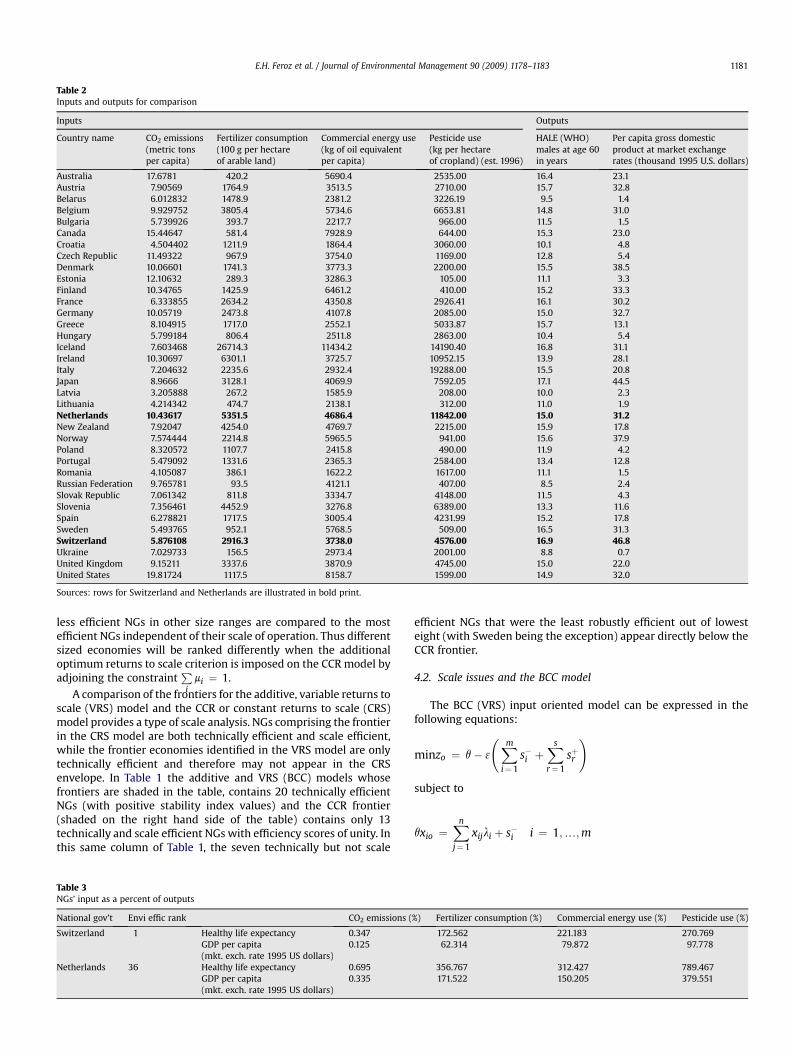
Table 2Inputs and outputs for comparison

Inputs Outputs

Country name CO2 emissions(metric tonsper capita)

Fertilizer consumption(100 g per hectareof arable land)

Commercial energy use(kg of oil equivalentper capita)

Pesticide use(kg per hectareof cropland) (est. 1996)

HALE (WHO)males at age 60in years

Per capita gross domesticproduct at market exchangerates (thousand 1995 U.S. dollars)

Australia 17.6781 420.2 5690.4 2535.00 16.4 23.1Austria 7.90569 1764.9 3513.5 2710.00 15.7 32.8Belarus 6.012832 1478.9 2381.2 3226.19 9.5 1.4Belgium 9.929752 3805.4 5734.6 6653.81 14.8 31.0Bulgaria 5.739926 393.7 2217.7 966.00 11.5 1.5Canada 15.44647 581.4 7928.9 644.00 15.3 23.0Croatia 4.504402 1211.9 1864.4 3060.00 10.1 4.8Czech Republic 11.49322 967.9 3754.0 1169.00 12.8 5.4Denmark 10.06601 1741.3 3773.3 2200.00 15.5 38.5Estonia 12.10632 289.3 3286.3 105.00 11.1 3.3Finland 10.34765 1425.9 6461.2 410.00 15.2 33.3France 6.333855 2634.2 4350.8 2926.41 16.1 30.2Germany 10.05719 2473.8 4107.8 2085.00 15.0 32.7Greece 8.104915 1717.0 2552.1 5033.87 15.7 13.1Hungary 5.799184 806.4 2511.8 2863.00 10.4 5.4Iceland 7.603468 26714.3 11434.2 14190.40 16.8 31.1Ireland 10.30697 6301.1 3725.7 10952.15 13.9 28.1Italy 7.204632 2235.6 2932.4 19288.00 15.5 20.8Japan 8.9666 3128.1 4069.9 7592.05 17.1 44.5Latvia 3.205888 267.2 1585.9 208.00 10.0 2.3Lithuania 4.214342 474.7 2138.1 312.00 11.0 1.9Netherlands 10.43617 5351.5 4686.4 11842.00 15.0 31.2New Zealand 7.92047 4254.0 4769.7 2215.00 15.9 17.8Norway 7.574444 2214.8 5965.5 941.00 15.6 37.9Poland 8.320572 1107.7 2415.8 490.00 11.9 4.2Portugal 5.479092 1331.6 2365.3 2584.00 13.4 12.8Romania 4.105087 386.1 1622.2 1617.00 11.1 1.5Russian Federation 9.765781 93.5 4121.1 407.00 8.5 2.4Slovak Republic 7.061342 811.8 3334.7 4148.00 11.5 4.3Slovenia 7.356461 4452.9 3276.8 6389.00 13.3 11.6Spain 6.278821 1717.5 3005.4 4231.99 15.2 17.8Sweden 5.493765 952.1 5768.5 509.00 16.5 31.3Switzerland 5.876108 2916.3 3738.0 4576.00 16.9 46.8Ukraine 7.029733 156.5 2973.4 2001.00 8.8 0.7United Kingdom 9.15211 3337.6 3870.9 4745.00 15.0 22.0United States 19.81724 1117.5 8158.7 1599.00 14.9 32.0

Sources: rows for Switzerland and Netherlands are illustrated in bold print.

E.H. Feroz et al. / Journal of Environmental Management 90 (2009) 1178–1183 1181

less efficient NGs in other size ranges are compared to the mostefficient NGs independent of their scale of operation. Thus differentsized economies will be ranked differently when the additionaloptimum returns to scale criterion is imposed on the CCR model byadjoining the constraint

Pi

mi ¼ 1.

A comparison of the frontiers for the additive, variable returns toscale (VRS) model and the CCR or constant returns to scale (CRS)model provides a type of scale analysis. NGs comprising the frontierin the CRS model are both technically efficient and scale efficient,while the frontier economies identified in the VRS model are onlytechnically efficient and therefore may not appear in the CRSenvelope. In Table 1 the additive and VRS (BCC) models whosefrontiers are shaded in the table, contains 20 technically efficientNGs (with positive stability index values) and the CCR frontier(shaded on the right hand side of the table) contains only 13technically and scale efficient NGs with efficiency scores of unity. Inthis same column of Table 1, the seven technically but not scale

Table 3NGs’ input as a percent of outputs

National gov’t Envi effic rank CO2 emissions (

Switzerland 1 Healthy life expectancy 0.347GDP per capita 0.125(mkt. exch. rate 1995 US dollars)

Netherlands 36 Healthy life expectancy 0.695GDP per capita 0.335(mkt. exch. rate 1995 US dollars)

efficient NGs that were the least robustly efficient out of lowesteight (with Sweden being the exception) appear directly below theCCR frontier.

4.2. Scale issues and the BCC model

The BCC (VRS) input oriented model can be expressed in thefollowing equations:

minzo ¼ q� 3

Xmi¼1

s�i þXs

r¼1

sþr

!

subject to

qxio ¼Xn

j¼1

xijli þ s�i i ¼ 1;.;m

%) Fertilizer consumption (%) Commercial energy use (%) Pesticide use (%)

172.562 221.183 270.76962.314 79.872 97.778

356.767 312.427 789.467171.522 150.205 379.551

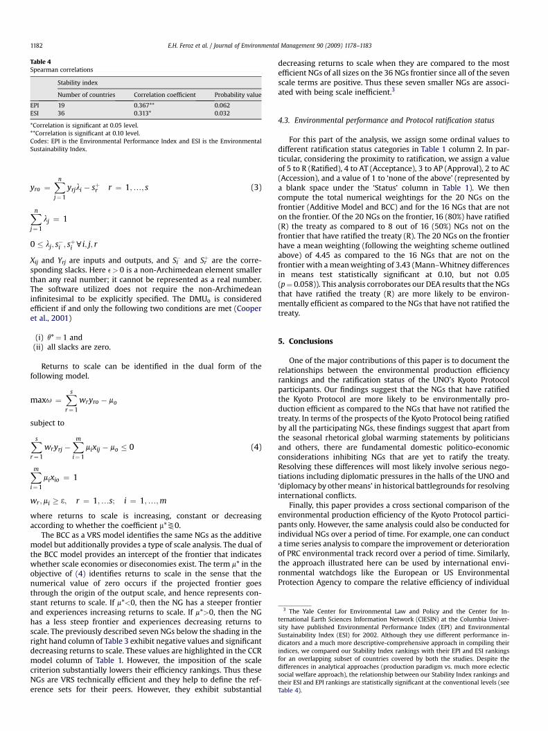
Table 4Spearman correlations

Stability index

Number of countries Correlation coefficient Probability value

EPI 19 0.367** 0.062ESI 36 0.313* 0.032

*Correlation is significant at 0.05 level.**Correlation is significant at 0.10 level.Codes: EPI is the Environmental Performance Index and ESI is the EnvironmentalSustainability Index.

3 The Yale Center for Environmental Law and Policy and the Center for In-ternational Earth Sciences Information Network (CIESIN) at the Columbia Univer-sity have published Environmental Performance Index (EPI) and EnvironmentalSustainability Index (ESI) for 2002. Although they use different performance in-dicators and a much more descriptive-comprehensive approach in compiling theirindices, we compared our Stability Index rankings with their EPI and ESI rankingsfor an overlapping subset of countries covered by both the studies. Despite thedifferences in analytical approaches (production paradigm vs. much more eclecticsocial welfare approach), the relationship between our Stability Index rankings andtheir ESI and EPI rankings are statistically significant at the conventional levels (seeTable 4).

E.H. Feroz et al. / Journal of Environmental Management 90 (2009) 1178–11831182

yro ¼Xn

j¼1

yrjli � sþr r ¼ 1;.; s (3)

Xn

j¼1

lj ¼ 1

0 � lj; s�i ; sþi ci; j; r

Xij and Yrj are inputs and outputs, and Si� and Sr

þ are the corre-sponding slacks. Here e> 0 is a non-Archimedean element smallerthan any real number; it cannot be represented as a real number.The software utilized does not require the non-Archimedeaninfinitesimal to be explicitly specified. The DMUo is consideredefficient if and only the following two conditions are met (Cooperet al., 2001)

(i) q*¼ 1 and(ii) all slacks are zero.

Returns to scale can be identified in the dual form of thefollowing model.

maxu ¼Xs

r¼1

wryro � mo

subject to

Xs

r¼1

wryrj �Xmi¼1

mixij � mo � 0 (4)

Xmi¼1

mixio ¼ 1

wr;mi � 3; r ¼ 1;.s; i ¼ 1;.;m

where returns to scale is increasing, constant or decreasingaccording to whether the coefficient m*X0.

The BCC as a VRS model identifies the same NGs as the additivemodel but additionally provides a type of scale analysis. The dual ofthe BCC model provides an intercept of the frontier that indicateswhether scale economies or diseconomies exist. The term m* in theobjective of (4) identifies returns to scale in the sense that thenumerical value of zero occurs if the projected frontier goesthrough the origin of the output scale, and hence represents con-stant returns to scale. If m*<0, then the NG has a steeper frontierand experiences increasing returns to scale. If m*>0, then the NGhas a less steep frontier and experiences decreasing returns toscale. The previously described seven NGs below the shading in theright hand column of Table 3 exhibit negative values and significantdecreasing returns to scale. These values are highlighted in the CCRmodel column of Table 1. However, the imposition of the scalecriterion substantially lowers their efficiency rankings. Thus theseNGs are VRS technically efficient and they help to define the ref-erence sets for their peers. However, they exhibit substantial

decreasing returns to scale when they are compared to the mostefficient NGs of all sizes on the 36 NGs frontier since all of the sevenscale terms are positive. Thus these seven smaller NGs are associ-ated with being scale inefficient.3

4.3. Environmental performance and Protocol ratification status

For this part of the analysis, we assign some ordinal values todifferent ratification status categories in Table 1 column 2. In par-ticular, considering the proximity to ratification, we assign a valueof 5 to R (Ratified), 4 to AT (Acceptance), 3 to AP (Approval), 2 to AC(Accession), and a value of 1 to ‘none of the above’ (represented bya blank space under the ‘Status’ column in Table 1). We thencompute the total numerical weightings for the 20 NGs on thefrontier (Additive Model and BCC) and for the 16 NGs that are noton the frontier. Of the 20 NGs on the frontier, 16 (80%) have ratified(R) the treaty as compared to 8 out of 16 (50%) NGs not on thefrontier that have ratified the treaty (R). The 20 NGs on the frontierhave a mean weighting (following the weighting scheme outlinedabove) of 4.45 as compared to the 16 NGs that are not on thefrontier with a mean weighting of 3.43 (Mann–Whitney differencesin means test statistically significant at 0.10, but not 0.05(p¼ 0.058)). This analysis corroborates our DEA results that the NGsthat have ratified the treaty (R) are more likely to be environ-mentally efficient as compared to the NGs that have not ratified thetreaty.

5. Conclusions

One of the major contributions of this paper is to document therelationships between the environmental production efficiencyrankings and the ratification status of the UNO’s Kyoto Protocolparticipants. Our findings suggest that the NGs that have ratifiedthe Kyoto Protocol are more likely to be environmentally pro-duction efficient as compared to the NGs that have not ratified thetreaty. In terms of the prospects of the Kyoto Protocol being ratifiedby all the participating NGs, these findings suggest that apart fromthe seasonal rhetorical global warming statements by politiciansand others, there are fundamental domestic politico-economicconsiderations inhibiting NGs that are yet to ratify the treaty.Resolving these differences will most likely involve serious nego-tiations including diplomatic pressures in the halls of the UNO and‘diplomacy by other means’ in historical battlegrounds for resolvinginternational conflicts.

Finally, this paper provides a cross sectional comparison of theenvironmental production efficiency of the Kyoto Protocol partici-pants only. However, the same analysis could also be conducted forindividual NGs over a period of time. For example, one can conducta time series analysis to compare the improvement or deteriorationof PRC environmental track record over a period of time. Similarly,the approach illustrated here can be used by international envi-ronmental watchdogs like the European or US EnvironmentalProtection Agency to compare the relative efficiency of individual

E.H. Feroz et al. / Journal of Environmental Management 90 (2009) 1178–1183 1183

member states or the relative efficiency of the same state or nationover a period of time.

References

Alsharif, K., Feroz, E.H., Klemer, A., Raab, R., 2008. Governance of the watersupply systems in the Palestinian territories: a data envelopment analysisapproach to the management of water resources. Journal of EnvironmentalManagement 87, 80–94.

Banker, R.D., Charnes, A., Cooper, W.W., 1984. Some models for estimating technicaland scale inefficiencies in data envelopment analysis. Management Science 30,1078–1092.

Charnes, A., Cooper, W.W., Rhodes, E., 1981. Evaluating program and managerialefficiency: an application of the data envelopment analysis to program followthrough. Management Science 27, 668–697.

Charnes, A., Cooper, W.W., Golany, B., Seiford, L., Stutz, J., 1985. Foundations of dataenvelopment analysis for Pareto-Koopmans efficient empirical productionfunctions. Journal of Econometrics 3, 91–107.

Cooper, W.W., Li, S., Seiford, L.M., Tone, K., Thrall, R.H., Zhu, 2001. Sensitivity andstability analysis in DEA: some recent developments. Journal of ProductivityAnalysis 15, 217–246.

Cooper, W.W., Seiford, L.M., Tone, K., 2007. Data Envelopment Analysis:a Comprehensive Text. Springer.

Raab, R.L., Feroz, E.H., 2007. A productivity growth accounting approach to theranking of the developing and developed nations. The International Journal ofAccounting 42, 396–415.

World Development Indicators 2001. International Bank for Reconstruction andDevelopment/The World Bank, 1818 H street NW, Washington, D.C. 20433USA.

World Economic Forum, Yale Center for Environmental Law and Policy, and CIESIN,2002. Environmental Sustainability Index.

World Health Organization, 1211 Geneva 27, Switzerland, 2002. World HealthReport, Table 4, Statistical Annex.