globalisation and deglobalisation - bis.org · papers in this volume were prepared for a meeting of...
TRANSCRIPT

BIS Papers No 100
Globalisation and deglobalisation
Monetary and Economic Department
December 2018
JEL classification: F60, F61, F62, F68

Papers in this volume were prepared for a meeting of senior officials from central banks held at the Bank for International Settlements on 8 – 9 February 2018. The views expressed are those of the authors and do not necessarily reflect the views of the BIS or the central banks represented at the meeting. Individual papers (or excerpts thereof) may be reproduced or translated with the authorisation of the authors concerned.
This publication is available on the BIS website (www.bis.org).
© Bank for International Settlements 2018. All rights reserved. Brief excerpts may be reproduced or translated provided the source is stated.
ISSN 1609-0381 (print) ISBN 978-92-9259-230-1 (print)
ISSN 1682-7651 (online) ISBN 978-92-9259-231-8 (online)

BIS Papers No 100 i
Contents
BIS background papers
Globalisation and deglobalisation in emerging market economies: facts and trends Yavuz Arslan, Juan Contreras, Nikhil Patel and Chang Shu .................................................... 1
How has globalisation affected emerging market economies? Yavuz Arslan, Juan Contreras, Nikhil Patel and Chang Shu ................................................. 27
Contributed papers
Globalisation, growth and inequality from an emerging economy perspective Central Bank of Argentina ................................................................................................................. 57
Globalisation and deglobalisation Central Bank of Brazil .......................................................................................................................... 71
Globalisation and the Chilean economy Joaquin Vial ............................................................................................................................................. 83
How globalisation has affected China and related policy issues The People’s Bank of China ............................................................................................................ 101
International trade networks and the integration of Colombia into global trade Andrés Murcia, Hernando Vargas and Carlos León .............................................................. 105
Foreign capital and domestic productivity in the Czech Republic Mojmír Hampl and Tomáš Havránek .......................................................................................... 125
Assessing the impact of globalisation: Lessons from Hong Kong Lillian Cheung, Eric Wong, Philip Ng and Ken Wong ........................................................... 139
The external and domestic drivers of inflation: the case study of Hungary Erzsébet Éva Nagy and Veronika Tengely ................................................................................ 149
Globalisation and deglobalisation: the Indonesian perspective Dody Budi Waluyo ............................................................................................................................. 173
Measuring the importance of global factors in determining inflation in Israel Nadine Baudot-Trajtenberg and Itamar Caspi ........................................................................ 183
Foreign workers in the Korean labour market: current status and policy issues Seung-Cheol Jeon .............................................................................................................................. 209
Globalisation and deglobalisation Central Bank of Malaysia ................................................................................................................. 223
Globalisation and consumption risk-sharing in emerging market economies Manuel Ramos-Francia and Santiago García-Verdú ............................................................ 231
Peru’s commercial opening: the story of two sectors Renzo Rossini, Zenon Quispe, Hiroshi Toma, Cesar Vasquez ........................................... 245
The globalisation experience and its challenges for the Philippine economy Diwa C Guinigundo ............................................................................................................................ 259
Globalisation and the Polish economy: macro and micro growth effects Piotr Szpunar and Jan Hagemejer ............................................................................................... 273

ii BIS Papers No 100
Globalisation and deglobalisation Bank of Russia ...................................................................................................................................... 291
Macroeconomic and distributional effects of globalisation Saudi Arabian Monetary Authority ............................................................................................. 311
Globalisation in a small open economy: the Singapore experience Edward Robinson ............................................................................................................................... 321
Globalisation and deglobalisation South African Reserve Bank ........................................................................................................... 331
Weighing up Thailand’s benefits from global value chains Bank of Thailand ................................................................................................................................. 345
Globalisation and deglobalisation Central Bank of the Republic of Turkey ..................................................................................... 355
List of participants .............................................................................................................................. 363
Previous volumes from Deputy Governors’ Meetings ......................................................... 365

BIS Paper 100 1
Globalisation and deglobalisation in emerging market economies: facts and trends
Yavuz Arslan, Juan Contreras, Nikhil Patel and Chang Shu
Abstract
This paper discusses different facts and trends with regard to globalisation in emerging market economies (EMEs). It focuses primarily on the real (as opposed to financial) side of the economy over the last 2-3 decades, and highlights important similarities and differences across countries with respect to trade, global value chains, foreign direct investment, and migration. It concludes with a discussion of the recent slowdown in the growth of global trade.
Keywords: Globalisation, international trade, migration, global value chains, foreign direct investment.
JEL classifications: F02, F15, F22

2 BIS Papers No 100
1. Introduction
Emerging market economies (EMEs) have become much more integrated into the world economy over the last few decades along several dimensions. Trade volumes, measured by exports plus imports in relation to GDP, more than doubled between early 1970 and 2016, due in part to declines in tariffs and transportation costs (Graph 1, left-hand panel). Financial integration followed with a delay, gaining momentum in the early 1990s.
Tighter trade and financial integration have increased the importance of EMEs in the global economy. But globalisation extends well beyond the flow of goods and services. Perhaps the most debated aspect of globalisation is the flow of people, at least in some advanced economies (AEs). But while migration (inward and outward) surged in several EMEs (eg Malaysia, Mexico, Saudi Arabia, Thailand and the United Arab Emirates) in recent decades, it fell in others. Overall, the share of migrants in the population has increased only slightly since 1960s (Graph 1, right-hand panel). Less tangible flows not easily captured by data, such as those in ideas and information, have also boosted integration substantially.1
This note discusses the various facets of globalisation from an EME perspective, focusing primarily on the real (as opposed to financial) side of the economy, especially in the last two decades.2 The emphasis is on summarising facts and trends and on differences across EMEs. A second note (Note 2) discusses the economic impact of globalisation and policy responses.
The remainder of the note is structured as follows. Section 2 discusses issues pertaining to trade globalisation and the rise of global value chains (GVCs). Section 3 provides an overview of trends in foreign direct investment. Section 4 describes migration flows and investigates their determinants. Section 5 discusses the main long-term determinants of globalisation in EMEs and explores possible reasons behind the recent slowdown.
1 See Baldwin (2016). He argues that even if foreign trade may have peaked relative to GDP and GVCs
have stopped growing, this less tangible form of globalisation will arguably continue, with important consequences for economic structures and welfare and for cross-border capital flows.
2 A first wave of globalisation finished with World War I and the Great Depression. Trade and financial openness of the major economies more than doubled from around 1800 to the end of that century. For a more detailed account, see BIS (2017), Chapter VI, which also discusses the interconnections between the real and financial aspects of globalisation.

BIS Paper 100 3
2. Trade
The share of EMEs in world trade has risen substantially in the last five decades, reflecting a pickup in their overall growth rate as well as tighter integration into the world economy (Graph 2, left-hand panel). While there has been a strong increase in overall trade openness in EMEs, there is a high degree of variation across countries (right-hand panel). Notably, Hong Kong SAR and Singapore have been by far the most open for a long time. The note by Hong Kong mentions how, driven by the economic and political environment, Hong Kong has long been a globalised economy. Singapore’s note mentions that due to the lack of natural resources and a natural economic hinterland, Singapore has had to depend on global markets, free trade and free capital flows.
Varying integration momentum across countries is another reason behind differing degrees of trade openness. EMEs in Southeast Asia have increased their trade openness rapidly, as most of them have long pursued an export-led growth model. In central and eastern Europe (CEE), integration into the global economy coincided first with the transition from a planned to a market economy and, later, with accession to the European Union (see note by Poland). Several EMEs in Latin America remain relatively closed even today (eg Argentina and Brazil) despite some liberalisation in the 1990s. In China, trade openness has increased rapidly since the
EMEs have integrated rapidly into the global economy Graph 1
Trade and financial globalisation trend upwards in EMEs1
Percentage of GDP
Migrant stocks Percentage of population
AE = United Arab Emirates; AR = Argentina; BR = Brazil; CL = Chile; CN = China; CO = Colombia; CZ = Czech Republic; DZ = Algeria; HK = Hong Kong SAR; HU = Hungary; ID = Indonesia; IL = Israel; IN = India; KR = Korea; MX = Mexico; MY = Malaysia; PE = Peru; PH = Philippines; PL = Poland; RU = Russia; SA = Saudi Arabia; SG = Singapore; TH = Thailand; TR = Turkey; ZA = South Africa.
1 Unweighted averages of AE, AR, BR, CL, CN, CO, CZ, DZ, HK, HU, ID, IL, IN, KR, MX, MY, PE, PH, PL, RU, SA, SG, TH, TR, ZA. 2 Sum of exports and imports of goods and services. 3 Sum of FDI inward and outward stocks.
Sources: UNCTAD; World Bank; Datastream; BIS calculations.

4 BIS Papers No 100
late 1970s, but because of the low starting point and the economy’s large size trade still accounts for a relatively small part of domestic output.
Large cross-country variation despite general integration into the global economy Graph 2
Contributions to world trade openness1
Openness in EMEs varies
Per cent Per cent of GDP
See Graph 1 for definitions of country codes.
1 Exports plus imports of country group divided by world GDP. 2 World total less the share of advanced economies. 3 For Czech Republic and Poland, 1990; for Hong Kong SAR, 1961; for Hungary, 1991; for Russia, 1989; for Saudi Arabia, 1968.
Sources: World Bank, World Development Indicators; Datastream; BIS calculations.
Despite more liberal trade policies and decreasing trading costs, distance and regional effects remain the key determinants of trade volume, in line with the gravity models of trade. For example, trade as measured by exports (imports) between AEs and EMEs in Europe is 3.1% (2.7%) of regional GDP, while that between AEs in Europe and EMEs in other regions is below 2% of the respective regional GDP. The same regional pattern holds for all EMEs (diagonal elements in left-hand panel of Table 1).3 Similarly, examining the relationship within different country pairs, Appendix 2 investigates the strength of bilateral trade linkages among different major EMEs, as captured by the ratio of total trade in the combined GDP of each country pair. It confirms that the gravity model of trade may be alive and well, and that physical distance still plays an important role in explaining cross-country trade patterns.
3 The negative impact of physical distance between countries on bilateral trade (as well as financial
flow) intensity has not declined over time. This remains somewhat of a puzzle in the academic literature. See eg Brei and von Peter (2017).

BIS Paper 100 5
Along with the considerable rise in its total volume, the composition and nature of trade have also changed substantially. In 1970, primary commodities accounted for approximately four fifths of total trade for a sample of EMEs. Manufactured goods made up much of the remaining quarter, while services were minuscule (Graph 3, left-hand panel). Some 45 years later, the picture has changed completely. While trade in primary commodities accounts for a similar proportion of GDP, it has been dwarfed by the growth in trade in manufactured goods and services. Together, in 2015 these two categories accounted for about 80% of total trade in EMEs. As trade volumes in manufactures grew, the nature of the goods also changed. EMEs have become much more integrated in international production networks and GVCs (right-hand panel). The next section discusses this phenomenon.
Bilateral trade links are widely spread
Inter-regional bilateral trade as a percentage of region-wide GDP Table 1
Trade links Changes in trade links
2015
Importers
AE OA EE EA LA AME
Expo
rter
s
AE 20.9 1.4 2.7 1.5 0.6 1.5 OA 1.0 7.7 0.2 1.9 1.3 0.5 EE 3.1 0.2 9.0 0.6 0.2 1.0 EA 1.9 2.8 0.8 12.0 1.0 1.6 LA 0.5 1.5 0.2 0.7 3.5 0.3 AME 1.1 0.6 0.4 2.0 0.2 5.4
Change between 2001 and 2015
Importers
AE OA EE EA LA AME
Expo
rter
s
AE 0.3 0.1 1.2 0.4 0.1 0.5
OA –0.1 –0.4 0.1 0.3 0.3 0.2
EE 1.5 0.1 2.6 0.1 0.1 0.6
EA 0.4 0.6 0.3 4.1 0.5 0.7
LA 0.1 0.3 0.1 0.4 0.2 0.1
AME 0.0 –0.0 0.1 0.5 0.0 2.5
Weaker link Stronger link
AEs: AE = advanced Europe; OA = other AEs.
EMEs: AME = Africa and Middle East; EA = emerging Asia; EE = emerging Europe; LA = Latin America.
In each cell, the numerator is calculated as the sum of individual countries’ bilateral trade links; the denominator is equal to the combined GDP of the two regions, adjusted to exclude any missing bilateral links.
Sources: IMF, Direction of Trade Statistics; UNCTAD, BIS calculations.

6 BIS Papers No 100
Trade has become more complex as GVCs have grown Graph 3
Composition of trade for EMEs1 GVC2 participation has increased in EMEs Percentage of regional GDP Per cent
1 Trade between EMEs and the rest of the world. EMEs: Bulgaria, Brazil, China, Chinese Taipei, Croatia, the Czech Republic, Hungary, India, Indonesia, Korea, Mexico, Poland, Romania, Russia, Turkey. 2 GVCs: sum of foreign value added content of exports and domestic value added sent to third economies, as a share of gross exports. Simple average of the countries.
Sources: OECD; World Bank; Datastream; BIS calculations.
Global value chains
A prominent feature of trade globalisation has been the rise of GVCs, at least until the Great Financial Crisis (GFC). Declining trade barriers and advances in communication and transportation technologies have allowed firms to split up production processes into various stages and locate them around the world to exploit differences in factor endowments and comparative advantage. This has resulted in long production chains that span multiple sectors over many countries, with intermediate goods shipped several times before finally becoming embodied in final goods for consumption. As discussed below, newly developed GVC metrics allow a more granular decomposition of domestic and cross-border production activities, shedding considerable light on the phenomenon.
The participation of EMEs in GVCs varies significantly across regions (Graph 4, left-hand panel).4,5 EMEs in CEE are even more integrated into GVCs than the average advanced economy, followed by those in Asia and Latin America.6 Complex GVC
4 Several recent studies have attempted to model the causes behind the differences in GVC
participation and positions across countries (see eg Antràs and de Gortari (2017). The note by the central bank of Russia also points out several factors such as location and unit costs that are positively related to GVC participation.
5 These numbers are based on the most recent release of the World Input-Output database, which covers 2000–14 at annual frequency.
6 As shown in Appendix 1, the higher levels of GVC participation and production lengths in CEE EMEs (discussed below) are not mere artefacts of their small size and large trade openness.

BIS Paper 100 7
participation (involving more than one border crossing) rose markedly across all regions between 2000 and 2014 (same graph), although the overall share of GVC-related trade has fallen.7
GVCs and production length Graph 4
GVC participation1 Average production length,2 2014
1 Simple GVC participation involves one border crossing; complex GVC participation involves more than one border crossing. 2 Red bars denote production length of GVC activities (goods crossing national borders for production purposes). Blue bars show the average number of border crossings involved in a typical GVC in the country group.
Sources: Wang et al (2017a,b); World Input-Output database; BIS calculations.
GVCs have also become longer, especially in Asia (Graph 4, right-hand panel).8 While GVCs in Asia involve the same number of border crossings as elsewhere, more of the processing stages take place within national borders.9 Longer GVCs are usually a sign of increasing specialisation and efficiency gains, but they can also be a source of vulnerability stemming from higher dependence on external finance (see box).
7 Although the fact that GVC data are available with a significant lag prevents a detailed examination
into the causes behind this fall, it is likely that the decline in the 2014 numbers is at least in part due to cyclical factors in the aftermath of the GFC and subsequent fall in commodity prices.
8 The length of GVCs can be measured in both a forward- and a backward-looking way. As an example, consider a three-country supply chain in which Japan exports raw materials to China, which combines them with its own labour and exports the final product to the United States. In this case, the forward-looking production length for Japan will is 2, and that for China is 1. Likewise, the backward-looking production length for the United States is 2. The graph plots the average of the two measures.
9 These patterns are robust to controlling for GDP and overall trade openness. See Appendix 1.

8 BIS Papers No 100
Truly global production chains, ie those that span regions, tend to be longer and more complex than those covering only one region or country. Table 2 provides a snapshot of production lengths between major EMEs and an aggregate advanced economy group. These numbers are generated from input-output tables based on the framework proposed in Wang et al (2017b), using a 56-sector classification in the World Input-Output Database. The numbers along a row can be interpreted as production lengths in a forward-looking sense, and those in the columns as production lengths in a backward-looking sense. For example, it takes 5.05 production stages on average before output from a Brazilian sector is embodied in final goods produced by an average Chinese sector (first row, third column), and 5.37 stages before Chinese output is embodied in Brazilian final goods (second row, first column). This is longer than the 4.06 (forward) and 3.95 (backward) stages involved in production chains with Mexico or the 1.63 of purely domestic chains.
The factor content of value added exports from EMEs tends to be more capital- and (low-skill) labour-intensive than that from AEs (red and yellow areas in Graph 5). Conversely, that of high-skill labour (blue areas) tends to be significantly lower. But there are a few notable exceptions. Korea and Hungary, for instance, have a high-skill share in line with that in advanced economies.10
10 In the case of Mexico, the high capital share reflects energy exports.
Bilateral production length, 2014 Table 2
BR MX CN ID IN KR CZ HU PL RU TR AEs
BR 1.6 4.1 5.1 4 4 4.8 5.6 4.8 4.8 4.5 4.2 4.3
MX 4.0 1.4 5.8 5.1 3.9 4.6 4.6 4.4 5.1 5.2 4.2 4.5
CN 5.4 5.1 2.7 5.1 5.6 5.4 5.3 5.1 5.5 5.4 5.4 5.5
ID 4.1 4.5 5.5 1.7 3.9 4.4 5.4 5.1 4.9 4.6 4 4.7
IN 4.3 4.4 5.8 3.9 1.6 4.8 4.7 4.7 4.6 4.6 3.9 4.4
KR 4.2 3.8 5.2 4 4.5 1.8 4.5 4 4.3 4.4 4.2 4.9
CZ 4.7 4.2 5.7 4.8 4.9 5 1.7 3.4 3.8 4 4 4.1
HU 4.5 3.7 5.6 5.3 5.2 4.6 3.4 1.4 3.6 4.1 3.8 3.8
PL 4.9 4.4 6.0 5.3 5.2 4.8 3.6 3.5 1.7 4 4 4.1
RU 5.4 5.7 6.3 5.1 5.3 5.5 4.2 4.7 4.0 1.8 4.3 4.7
TR 4.4 4.3 6.4 4.2 4.8 5.6 4.3 3.8 4.1 3.8 1.6 4.3
AEs 4.4 4.4 5.8 4.8 4.9 4.9 4.4 4.1 4.3 4.6 4.3 1.6
Shorter Longer
The numbers along a row can be interpreted as production lengths in a forward-looking sense, and those in the columns as production lengths in a backward-looking sense. See Graph 1 for definitions of country codes.
Sources: Wang et al (2017b); World Input-Output database; BIS calculations.

BIS Paper 100 9
Financial shocks and GVCs
Long production chains are more efficient but may be more susceptible to shocks. Production processes involving multiple shipments of goods across borders tend to take more time and require larger inventories at any point in time. This can make them vulnerable to disruptions, for instance to financial shocks that affect the availability of credit and working capital. Indeed, theoretical work by Bruno et al (2018) indicates that longer production chains are particularly sensitive to changes in financial conditions.
This box investigates the sensitivity of long production chains to financial factors by using sector-level measures of GVC production lengths developed by Wang et al (2017b). Production length is measured on a simple average count basis. As an example, consider a three-country supply chain in which Japan exports raw materials to China, which combines them with its own labour and exports the final product to the United States. In this case, the average forward-looking production length for Japan is 2 and that for China is 1. Likewise, the average backward-looking production length for the United States is 2. Wang et al (2017b) generalise and formalise this idea to compute the different components of average production lengths described in columns (2) and (3) in Table A.
We estimate the following panel regression to quantify the impact of a tightening of financial conditions on different measures of production lengths
,, , , , ,, ,c s t c t c s tt cc ss tY EMBI X θ= β + γ + ∂ + + ε
, , , , ,, ,c s t t c s t cc s t s tXY DollarREER θ= β + γ + ∂ + + ε
𝑌𝑌𝑐𝑐,𝑠𝑠,𝑡𝑡 denotes an average production length measure for sectors in country c at time t. 𝐸𝐸𝐸𝐸𝐸𝐸𝐸𝐸𝑐𝑐 ,𝑡𝑡 is the country-specific EMBI spread, DollarREER denotes the broad dollar index, given by the US real effective exchange rate. Both serve as proxies for global financial conditions. 𝑋𝑋𝑐𝑐,𝑠𝑠,𝑡𝑡 is a vector of control variables that includes the share of capital, high-skill and medium-skill labour in total production, the GDP deflator and CPI inflation (current and lagged value), the policy rate (contemporaneous and first difference), real GDP (level and growth rate) and value added and gross output (level and growth rate). The regressions also include country-sector fixed effects [ ,c s∂ ] and time fixed effects [ tθ ]. The results are robust to the inclusion of additional controls, such as sectoral value added exports (to control for the overall impact of financial conditions on trade) and various GVC participation measures.
Factor content in exports1
Share of capital and different labour components in the value added of exports Graph 5
See Graph 1 for definitions of country codes.
Sources: Wang et al (2017a); World Input-Output Database; BIS calculations.

10 BIS Papers No 100
The sample is annual and covers the period 1995–2009. It includes 35 sectors in 10 EMEs (see Table A notes for details). Column (2) in Table A summarises the sample mean for each measure of production length (taken to be the average of the respective forward- and backward-looking measure).
Response of production lengths to financial tightening Table A
(1) (2) (3) (4)
Response to 1 % pt increase
Length of production activities
Sample mean Sample mean of yearly changes (modulus)
EMBI spread dollar REER
Total 2.11 0.035 –0.0028* –0.0000
Domestic 1.76 0.037 –0.0035** –0.0004
Traditional trade 1.92 0.044 –0.0060*** 0.0011
GVC 4.04 0.053 –0.0088*** –0.0022**
The annual sample from 1995 to 2009 includes 35 sectors in 10 EMEs (Brazil, China, Hungary, India, Indonesia, Korea, Mexico, Poland, Russia and Turkey). See World Input-Output Database (www.wiod.org) for details on sectoral classification. Traditional trade includes goods produced domestically without using imported inputs, and shipped to a foreign country for final consumption, while GVC activities involve goods crossing national borders for production purposes. The production length measures used in the regressions are a simple average of the corresponding forward- and backward-looking production lengths (see Wang et al (2017b) for details). All left hand-side variables are winsorised at the 1% and 99% level to reduce the influence of outliers. “EMBI spread” denotes the country specific EMBI spread. “dollar REER” denotes the US real effective exchange rate.
*** p<0.01, ** p<0.05, * p<0.1 (based on robust standard errors clustered at the country level). The list of controls includes share of capital, high-skill and medium-skill labour, GDP deflator and CPI inflation (current and lagged value), policy rate (contemporaneous and first difference), real GDP (level and growth rate), sectoral value added and gross output (level and growth rate), policy rate (level and first difference). Country-sector fixed effects and time fixed effects are also included in each regression.
As shown in column (4) of Table A, measures of production length contract significantly in response to a worsening in financial conditions as measured by a rise in EMBI spreads. Moreover, this pattern is evident for all the segments of production, including those for traditional trade (goods produced domestically without using imported inputs, and shipped to foreign country for final consumption) as well as GVC activities (goods crossing national borders for production purposes). Due to the lack of variation within a year, the results are less strong if the US dollar effective exchange rate is used as a proxy for financial conditions (the sample is only 15 years), but the contraction in GVC length is still significant. In terms of magnitude, the impact of a 1 percentage point rise in the EMBI spread is about a 10th of the average yearly change (comparing columns (3) and (4)). Since the EMBI spread increased on average by about 9 percentage points across the countries in the sample between 2006 and 2009, financial factors alone can account for up to one third of the average change in production lengths according to these results. (The fact that the data end in 2009 precludes a more detailed analysis of the impact of the GFC on lengths of production chains, which continue to rise rather than fall through the sample period in this database. The limited sample (10 years) also precludes an analysis of the long-run implications of these results.)
To summarise, the empirical analysis above offers evidence indicating that production chains shorten in response to a tightening in financial conditions. Overall, these results highlight an important source of vulnerability stemming from long production chains in EMEs, and corroborate the results of Bruno et al (2018).
3. Foreign direct investment
Foreign direct investment (FDI) has surged since the mid-1990s in EMEs in all major regions (Graph 6, left-hand panel), increasing both as a ratio of GDP and as a share

BIS Paper 100 11
of total gross external liabilities (right-hand panel). Improvements in institutional quality and governance as well as better long-run macroeconomic conditions have been particularly important, and lighter regulation is also likely to have played a major role (Graph 6, centre panel). In general, countries with larger markets are more likely to attract FDI (IMF (2003)). While EMEs on average are net recipients, more recently outward FDI from EMEs has also become sizeable (around 15% of total FDI flows).11
11 The note by the central bank of Chile points out how the limited size of the domestic market led
Chilean firms to expand abroad.
FDI has been growing rapidly Graph 6
Regional FDI dynamics FDI restrictiveness Evolution of external positions Percentage of GDP 0 (open) to 1 (closed) Gross external liabilities as a % of GDP
See Graph 1 for definitions of country codes.
1 For the time periods in which “other investment debt” is plotted, the difference between total debt and other investment debt is primarily “portfolio debt”, although there is also a small unallocated debt residual.
Sources: Lane and Milesi-Ferretti (2017); OECD, FDI Regulatory Restrictiveness Index; UNCTAD; BIS calculations.

12 BIS Papers No 100
EME employment growth in US multinationals has been strong
In thousands of employees Graph 7
High US employment Low US employment
See Graph 1 for definitions of country codes.
Sources: OECD; BIS calculations.
FDI is perhaps the most praised aspect of globalisation. It is regarded as a major
driver of growth and development in EMEs (see eg the notes by Poland and Russia).12 But in practice FDI does not just cover greenfield investment, where a foreign firm sets up an affiliate and (ideally) transfers capital and skills to the new establishment. FDI flows also include purchases of domestic firms by foreigners and lending to affiliates.13 A large part of the recent rise in FDI reflects positions vis-à-vis financial centres (Avdjiev et al (2014); Gruić et al (2014)), so that the increase should be interpreted with caution (Lane and Milesi-Ferretti (2017)). That said, FDI measures that relate more to non-financial flows still suggest strong momentum. One such measure is employment in multinational companies (Graph 7). Since the early 1990s, employment growth in US multinational companies has been particularly strong in China, India and the Philippines, and robust in others as well.
4. Migration
The increasing flow of migrants across countries over the past few decades has perhaps been the most controversial aspect of globalisation. Many factors have
12 It also tends to be the most stable source of external financing for most EMEs, one that is also less
sensitive to business cycle fluctuations (Loungani and Razin (2001)).
13 Balance of payments statistics consider intra-company loans as FDI. The rationale is that this kind of debt does not come with hard obligations, as when the promise is made to an external party. While this share is typically small for EMEs (less than a third of total FDI), Avdjiev et al (2014) show that for some large EMEs like Brazil, China and Russia, this share is larger, and is comparable to the size of total portfolio inflows.

BIS Paper 100 13
facilitated migration. Prominent ones include: differences in economic conditions; geopolitical developments; lower travel cost; less stringent visa requirements and border controls; and tighter trade and financial linkages. According to the United Nations, the total number of immigrants across the world has more than doubled in the last three decades, from 104 million in 1985 to 234 million in 2015 (Graph 8, left-hand panel). And the official data likely substantially underestimate the scale and possibly the growth of immigration, as it does not cover the large number of undocumented immigrants. Nonetheless, there are signs that the growth in migration has slowed in the last decade. A narrowing gap in economic prospects between the recipient and source countries as well as rising anti-globalisation and anti-immigration sentiment may have contributed to this trend.
Migration flows have been unbalanced across the world, with EMEs mostly experiencing net emigration and advanced economies net immigration (Graph 8, left-hand panel). The scale of immigration to EMEs was comparable to that to AEs in 1990, but it has barely increased in the last three decades. In the meantime, EMEs saw faster growth in population outflows, leading to a rise in net outward migration from 2.7% to 6.3% of the population between 1990 and 2015. Among different regions, emerging Latin America and Europe experienced higher net outflows than emerging Asia (with the Philippines being an important exception), in part reflecting high growth and rising living standards in the latter group (right-hand panel).
EMEs saw net migration outflows Graph 8
World migration1 Net immigration rate2 Per cent Millions Per cent
1 Immigration is shown as positive values and emigration as negative values. 2 Net immigrants as a percentage of the population in the country of origin.
Sources: United Nations; World Bank.
Economic incentives as well as physical proximity between the source and destination countries are the major determinants of bilateral migration. Consistent with this, migration most commonly takes place within the same region, both among economies with similar levels of economic development and from EMEs to AEs (Table 3, bottom left-hand panel, row 3). Cross-regional movements tend to reflect
14 BIS Papers No 100
migration from EMEs to AEs as well as between AEs. By contrast, there is limited migration from AEs to EMEs even in the same region, and even less between regions.
The net outflows from EMEs to AEs are primarily driven by economic factors, although social and geopolitical factors are also important. For instance, unrest in some Middle Eastern countries in recent years has led to large-scale migration to Europe. More recently, the economic crisis in Venezuela has triggered large flows of migrants to the neighbouring economies and the Southern Cone.
Bilateral migration flows display a positive correlation with trade and financial linkages (Tables 1 and 3, left-hand panels).14 In addition, the intensities of trade, financial and migrant flows are all higher within a region than across regions, pointing to the importance of gravity factors (including distance, shared language and culture).
That said, there are also some important differences in patterns with regard to the three types of links – goods, finance and people. Trade flows are more diffuse and balanced than financial and migration flows, reflected by the often comparable sizes of imports and exports between regions (Table 1, left-hand panel). By contrast, while two-way financial flows also take place between EMEs, they principally occur between AEs and from AEs to EMEs. Migration flows are even less diffuse and balanced than financial flows, and have shown little change in the past two decades (Table 3, right-hand panel).
14 See BIS, 87th Annual Report, 2017, Chapter VI for detailed discussions on trade and financial links.

BIS Paper 100 15
5. Determinants of globalisation
What are the main factors that explain the trends in globalisation in EMEs in the past few decades as documented above? Has globalisation reached its limits? Why does the degree of integration vary so much across countries?
Probably the most important factor behind globalisation has come from the reduction in protectionist measures. Indeed, several central bank notes point to a consensus that export-led growth models have outperformed import substitution
Migration linkages are less balanced than trade and financial linkages
Table 3
Financial links
2015
Borrowers
AE OA EE EA LA AME
Lend
ers
AE 86.2 23.6 7.6 4.5 5.9 5.3
OA 20.5 31.0 0.7 4.1 4.1 2.1
EE 2.1 0.3 1.8 0.2 0.1 0.0
EA 0.9 1.7 0.3 2.4 0.3 0.8
LA 0.7 1.0 0.0 0.0 1.5 0.0
AME 3.5 2.0 0.5 0.5 0.3 5.5
Change between 2001 and 2015 Borrowers
AE OA EE EA LA AME
Lend
ers
AE 31.5 8.4 4.8 2.6 1.9 2.6
OA 7.7 17.9 0.4 2.3 1.7 1.4
EE 1.6 0.1 1.2 -0.0 0.1 -0.0
EA 0.3 1.0 0.3 0.2 0.2 0.6
LA 0.6 0.7 0.0 0.0 0.6 0.0
AME 2.2 1.7 0.4 0.5 0.3 4.4
Immigration
2015 Destination
AE OA EE EA LA AME
Orig
in
AE 1.4 0.5 0.2 0.0 0.1 0.0
OA 0.2 0.3 0.0 0.0 0.1 0.0
EE 2.0 0.4 1.5 0.1 0.0 0.0
EA 0.2 0.4 0.2 0.3 0.0 0.4
LA 0.4 2.0 0.0 0.0 0.4 0.0
AME 0.6 0.2 0.1 0.0 0.0 0.9
Change between 2001 and 2015 Destination
AE OA EE EA LA AME
Orig
in
AE 0.2 -0.1 0.0 0.0 0.0 0.0
OA 0.0 0.0 0.0 0.0 0.0 0.0
EE 0.8 0.0 -0.1 0.0 0.0 0.0
EA 0.1 0.1 0.0 0.0 0.0 0.2
LA 0.3 0.3 0.0 0.0 0.1 0.0
AME 0.1 0.1 0.1 0.0 0.0 0.0
Weaker link Stronger link
AEs: AE = advanced Europe; OA = other AEs.
EMEs: AME = Africa and Middle East; EA = emerging Asia; EE = emerging Europe; LA = Latin America.
For trade and financial links, in each cell, the numerator is calculated as the sum of individual countries’ bilateral (financial or trade) links; the denominator is equal to the combined GDP of the two regions, adjusted to exclude any missing bilateral links.
Sources: IMF, Coordinated Portfolio Investment Survey and Direction of Trade Statistics; United Nations; UNCTAD, Foreign Direct Investment Statistics; BIS locational banking statistics; BIS calculations.

16 BIS Papers No 100
ones (eg the notes by Argentina, Chile and Peru). Many EMEs in Asia adopted export-led growth models as far back as the early 1960s, opening their economies and experiencing high growth rates. By contrast, trade liberalisation in Latin America came relatively late. Chile radically liberalised its foreign trade (and other parts of the economy) as early as 1975, but partly reversed course after the severe crisis in the early 1980s (see note). Trade liberalisation attempts in other Latin American countries also stalled after the debt crisis, and most Latin American economies liberalised their economies only in the late 1980s/early 1990s, triggering large increases in foreign trade. These varied experiences suggest that removal of regulatory barriers has probably been the primary source of globalisation.
Trade barriers have declined Graph 9
Effectively applied weighted average tariff
Share of transactions facing burdensome non-tariff measures, by destination1
Trade volume-weighted trade costs2
Ad valorem freight transportation costs3
Per cent Per cent In the ad valorem equivalent Percentage of value shipped
1 A transaction is a pair of exported product (at HS6 level) and partner country for a company based on a survey of 8,100 companies from across 26 sectors in the EU’s 28 member states. 2 Includes all costs involved in trading goods internationally with another partner relative to those involved in trading goods domestically. In addition to transport costs and tariffs this covers direct and indirect costs associated with differences in languages, currencies as well as cumbersome import or export procedures (see Anderson and van Wincoop (2004)). 3 Fitted ad valorem rate derived from a regression, controlling for changes in the mix of trading partners and products traded.
Sources: Hummels (2007); International Trade Centre and European Commission (2016); IMF, Direction of Trade Statistics; UN ESCAP; BIS calculations.
Differences in the degree and nature of liberalisation policies are evident across countries. For instance, the notes by Malaysia, Peru, the Philippines and Russia identify free trade agreements as the major factor. Large tariff reductions outside trade agreements have also contributed to trade integration in a big way (see eg the notes by Chile and Peru). Average tariffs declined from around 20% in the early 1990s to less than 5% in the last decade (Graph 9, first panel). That said, tariff rates vary significantly across countries: from above 8% in Algeria and Brazil to almost zero in Singapore. Non-tariff measures were lowered as well, and vary across countries (second panel).

BIS Paper 100 17
Time and dollar costs of border and documentary compliance Graph 10
Time cost Dollar cost OECD Service Trade Restrictiveness Index
Hours USD 0 (least) to 1 (most restrictive)
See Graph 1 for definitions of country codes.
Sources: OECD, Service Trade Restrictiveness Index; World Bank, Doing Business Indicators.
Declining trade costs have no doubt been another major driver of globalisation. Ad valorem trade costs fell by about 10% between 1995 and 2006 in both EMEs and AEs (Graph 9, third panel). Data on earlier periods are sketchier but also point to falling trade costs. Data from France, the United Kingdom and the United States show an average 15% decline from 1950 to 1995 (Jacks et al (2008)). An important component is transportation costs, which have declined sharply since the late 1970s. In the mid-1970s, freight costs accounted for 13% of the value of goods shipped into the United States by air; by the late 1990s, this had fallen below 8%.15 Over the same period, the share of ocean freight costs fell from 10% to less than 6% (Graph 9, fourth panel). While these large cost reductions may still not be big enough to fully explain the increase in trade, they do not include others, for instance the quicker delivery and improved reliability linked to the containerisation of transportation (Baldwin (2016)).16
Despite large declines, EME trade barriers are still higher on average than those of AEs, suggesting scope for further reductions. One example relates to border and documentary compliance (Graph 10). In EMEs, on average, the time cost of border and documentary compliance is more than 100 hours, much higher than in AEs (left-hand panel). Similarly, the associated dollar cost in EMEs is more than twice that in AEs (centre panel).17 There is also large variation across countries. In addition, exporting costs are lower than importing costs, implying an implicit export subsidy.
15 It should be reasonable to assume that the decline in transportation costs for AEs also reflects a
similar decline in transportation costs for EMEs.
16 Despite improvements, Hummels (2007) estimates that goods imported into the United States by sea spend 20 days on a vessel.
17 Domestic transportation costs (both time and dollar) are also large for some countries. These are not reported as they are not comparable across countries.
18 BIS Papers No 100
While services trade has increased substantially, regulatory restrictions remain a roadblock. The OECD Services Trade Restrictiveness Index compiles a series of restrictions for 22 sectors in 44 countries.18 Overall, both EMEs and AEs have widespread restrictions on services trade (scores between 0.2 and 0.3 represent quite significant restrictions). But EMEs have more restrictions than AEs, and there is considerable variation among them (Graph 10, right-hand panel).
Most of the factors mentioned in this section relate directly to trade but have indirect effects on other aspects of globalisation. For instance, a boost in trade due to such policies will probably increase financial flows (BIS (2017)). Besides, the removal of some restrictions on trade has coincided with that of restrictions on other aspects. For example, Chilean and Russian experiences mentioned in those countries’ notes suggest that lower tariffs were implemented together with lower restrictions on FDI.
What explains the recent trade slowdown?
Trade volumes appear to have plateaued after recovering from their GFC-induced collapse, although there are signs of a recent pickup (WTO (2017) and Graph 11, left-hand panel).19 This represents a stark reversal of the long-standing trend of trade growth consistently outpacing GDP growth from the mid-1800s, with only a handful of exceptions such as the world wars and the interwar years. Initially, the trade growth slowdown was accounted for by AEs, especially in the euro area, but more recently it has been mainly concentrated in EMEs (Graph 11, right-hand panel).
18 These restrictions include limits on foreign equity, nationality of board of directors, licensing
requirements, cross-border mergers and acquisitions, capital controls, work permit requirements, entry visa quotas, duration of stay for foreign persons providing services as intra-corporate transferees, etc.
19 Many studies analyse the fall and subsequent weakness in trade, including Baldwin (2009), Constantinescu et al (2015, 2017), ECB (2016), Hoekman (2015), IMF (2016) and Haugh et al (2016).

BIS Paper 100 19
World trade growth exceeded world GDP growth until recently Graph 11
World trade growth and GDP growth World import growth decomposition1 Per cent Per cent
1 Weighted average of the economies cited, based on GDP and PPP exchange rates; IMF WEO forecasted values for 2016. 2 Euro area 19. 3 Chinese Taipei, Hong Kong SAR, India, Indonesia, Korea, Malaysia, the Philippines, Singapore and Thailand. 4 Argentina, Brazil, Chile, Colombia, the Czech Republic, Hungary, Mexico, Peru, Poland, Russia, Saudi Arabia, South Africa and Turkey. 5 Australia, Canada, Denmark, Japan, Norway, Sweden, Switzerland and the United Kingdom.
Sources: IMF, World Economic Outlook; OECD, Economic Outlook.
There could be several reasons for the post-crisis slowdown in global trade values.20 First, it could reflect temporary (cyclical) factors like weak aggregate demand (eg Ollivaud and Schwellnus (2015) and Veenendaal et al (2015)). If this were the case, both trade and demand should recover as the economic outlook brightens. A related issue is the slower recovery of (trade-intensive) investment with respect to (less trade-intensive) consumption around the world. There is some evidence for these factors playing a role in AEs, but they cannot explain what has happened in EMEs (Graph 12, left-hand panel). That said, recent data and upgrades to forecasts of trade growth by the World Trade Organization do offer some support for the view that the slowdown is largely cyclical in nature (WTO (2017))
Weakness in global trade could also reflect a more structural decline in the elasticity of trade values with respect to demand, a factor observed in EMEs as well as in the world (Graph 12, centre panel).21 This trend, in turn, can be linked to long-term changes in production technologies or consumer preferences (Constantinescu et al (2015)). One possible example is the structural shift from manufacturing to services, which are less trade-intensive. In fact, in some countries like China an integral part of the policy agenda is to accelerate this transition. Another possibility, stressed by Kee and Tang (2016), is that the build-up of physical and human capital is allowing
20 See, for example, the 2016 IMF World Economic Outlook.
21 The world’s output elasticity of trade has declined about 40% from its peak, similar to the magnitude observed in EMEs. The graph displays short-run elasticity. Long-run elasticity (not reported) shows a similar pattern. See Constantinescu et al (2015) for similar inference on the decline of trade elasticity.

20 BIS Papers No 100
China (and some other EMEs) to substitute imported for locally produced parts (Graph 12, right-hand panel). Slower expansion of GVCs might also help to explain the decline in global trade.
There may be several reasons behind stalling GVC lengths. Efficiency gains from fragmenting production may be nearing their limits, and wage increases in EMEs may have decreased the benefits of doing so. In addition, as argued earlier, in recent years transportation costs have increased and the reduction in trade tariffs has slowed. This may prevent the opening of new markets for final goods, and at the same time make it harder to reconfigure existing GVCs towards developing countries with abundant labour and lower wage costs. In addition to these structural causes, escalation of financial frictions in the aftermath of the GFC may also have been an important factor behind the decline in GVC lengths, as shown in the box. However, since this trend is relatively recent, and GVC data are only available with a significant lag, the jury is still out.22
22 As Brazil mentions in its country note, further expansion of GVCs could help revive trade if the digital
revolution allows small and medium-sized enterprises to access global markets and expand global services trade.
Cyclical and structural factors drive weak global trade Graph 12
Post-2008 recovery of capital goods has been weak in EMEs
EMEs output elasticity of trade – rolling estimates1
Domestic value added in exports of final products
log USD thousands Percentage of gross exports
1 The elasticity of world trade to world GDP is estimated with the following regression: Δln(trade)(t) = 𝛼𝛼 + 𝛽𝛽ln(GDP)(t-1)+ 𝛿𝛿ln(trade)(t–1) + 𝜆𝜆Δln(GDP)(t) + 𝜀𝜀(t), , where the short-run elasticity is given by λ and the long-run elasticity is given by –𝛽𝛽 /𝛿𝛿. Dashed lines show the 90% confidence bands. Time variation in the coefficients is obtained by running for each year to a regression using observations weighted by a Gaussian distribution centred on year y. 2 Simple average of Australia, Austria, Belgium, Canada, Denmark, Finland, France, Germany, Ireland, Italy, Japan, the Netherlands, New Zealand, Norway, Portugal, Spain, Sweden, Switzerland, the United Kingdom and the United States. 3 Simple average of Argentina, Brazil, Bulgaria, Cambodia, Chile, Chinese Taipei, Colombia, Costa Rica, Croatia, the Czech Republic, Hong Kong SAR, Hungary, India, Indonesia, Israel, Korea, Malaysia, Mexico, the Philippines, Poland, Romania, Russia, Saudi Arabia, Singapore, South Africa, Thailand, Tunisia, Turkey and Vietnam.
Sources: OECD, Economic Outlook; OECD, STAN; OECD, Trade in Value Added; US FFIEC; BIS calculations.
BIS Paper 100 21
Still, it is not clear that these structural changes are able to explain the full extent of the sharp post-crisis trade slowdown. One possibility is that the rapid trade growth before the GFC itself represented a bubble, made possible by ample global liquidity which encouraged longer GVCs. If this is true, what we are seeing now is just the return to something more normal.
References
Anderson, J, E and E Van Wincoop (2004): “Trade costs”, Journal of Economic Literature, 42(3), pp 691-751.
Antràs, P and A de Gortari (2017): “On the geography of global value chains”, NBER Working Papers, no 23456.
Avdjiev, S, M Chui and H S Shin (2014): “Non-financial corporations from emerging market economies and capital flows”, BIS Quarterly Review, December, pp 67–77.
Baldwin, R (ed) (2016): The great convergence, Harvard University Press.
Bank for International Settlements (2017): 87th Annual Report.
Brei, M and G von Peter (2017): “The distance effect in banking and trade”, Journal of International Money and Finance, vol 81, pp 116–37.
Bruno, V, S J Kim and H S Shin (2018): “Exchange rates and the working capital channel of trade fluctuations”, AEA Papers and Proceedings, January.
Constantinescu, C, A Mattoo and M Ruta (2015): “The global trade slowdown: cyclical or structural?”, World Bank Group Policy Research Working Papers, no 7158.
Constantinescu, C, A Mattoo and M Ruta (2017): “Does vertical specialization increase productivity?”,World bank Group Policy Research Working Papers no 7978
Dutt, P, A Santacreu and D Traca (2015): The gravity of experience.
ECB (2016): “Understanding the weakness in global trade: What is the new normal?”, European Central Bank Occasional Paper Series no 178.
Gruić, B, C Upper and A Villar (2014): “What does the sectoral classification of offshore affiliates tell us about risks?”, BIS Quarterly Review, December, pp 20–1.
Guinigundo, D (2017): “The advanced and challenges of globalisation in the Philippine economy”, country paper.
Haugh, D., A. Kopoin, E. Rusticelli, D. Turner, and R. Dutu (2016): “Cardiac Arrest or Dizzy Spell: Why is World Trade So Weak and What Can Policy Do About It?” Organization of Economic Cooperation and Development Economic Policy Paper no 18
Hoekman, B. (2015): “The Global Trade Slowdown. A New Normal?”, VoxEU ebook, London: CEPR Press and EUI
Hummels, D (2007): “Transportation costs and international trade in the second era of globalization”, Journal of Economic Perspectives, vol 21, no 3, pp 131–54.
IMF (2016): “Global trade: What´s behind the slowdown?” Chapter 2 in IMF World Economic Outlook (WEO), October 2016.

22 BIS Papers No 100
IMF (2003): “Foreign direct investment in emerging market countries”, Report of working group of capital markets consultative group.
International Trade Centre and European Commission (2016): Navigating non-tariff measures: insights from a business survey in the European Union.
Jacks, D,S, C M Meissner and D Novy (2008): “trade Costs, 1870-2000”, The American Economic Review, vol 98, no 2, pp 529-534. Centre for Economic Policy Research, pp 161–78.
Kee, H L and H Tang (2016): “Domestic value added in exports: Theory and firm evidence from China”, American Economic Review, vol 106, no 6, pp 1402–36.
Lane, P and G Milesi-Ferretti (2017): “International financial integration in the aftermath of the global financial crisis”, IMF Working Papers, no WP/17/115.
Loungani, P and A Razin (2001): ”How beneficial is foreign direct investment for developing countries?”, Finance and Development, vol 38, no 2.
Ollivaud, P and C Schwellnus (2015): “Does the post-crisis weakness of global trade solely reflect weak demand?”, OECD Economics Department Working Papers, no 1216.
Veenendaal, P, H Rojas-Romagosa, A Lejour and H Kox (2015): “A value-added trade perspective on recent patterns in world trade”, in B Hoekman (ed), The global trade slowdown: a new normal?, Centre for Economic Policy Research, pp 161–78.
Wang, Z, S J Wei, X Yu and K Zhu (2017a): “Measures of participation in global value chains and global business cycles”, NBER Working Papers, no 23222.
Wang, Z, S J Wei, X Yu and K Zhu (2017b): “Characterizing global value chains: production length and upstreamness”, NBER Working Papers, no 23261.
World Trade Organisation (2017): “Trade statistics and outlook”, press release, www.wto.org/english/news_e/pres17_e/pr800_e.pdf.

BIS Paper 100 23
Appendix 1: Global value chain integration – the role of size and overall trade openness
Table A1 reports the residuals from the following panel regression of different GVC measures on real GDP and trade openness.
𝐺𝐺𝐺𝐺𝐶𝐶𝑚𝑚𝑚𝑚𝑚𝑚𝑠𝑠𝑚𝑚𝑚𝑚𝑚𝑚𝑖𝑖,𝑡𝑡 = α + δ ln �𝑡𝑡𝑡𝑡𝑡𝑡𝑡𝑡𝑡𝑡𝐺𝐺𝐺𝐺𝐺𝐺
�𝑖𝑖,𝑡𝑡
+ β ln(𝐺𝐺𝐺𝐺𝐺𝐺)𝑖𝑖,𝑡𝑡 + 𝜀𝜀𝑖𝑖𝑡𝑡
A positive number indicates that the particular GVC measure for the recipient country group is higher than what would be predicted solely based on its overall size and trade openness; a negative number indicates the opposite. As is clear from the bottom row, measures of GVC integration are higher for central and eastern European countries even after accounting for their smaller size (with the exception of GVC production lengths).
Difference between actual and predicted GVC indicators Table A1
GVC simple GVC complex Production length
total Production length GVC
Advanced economies –0.03 –0.21 –2.82 –4.18
EMEs
Asia –0.42 –0.09 6.8 28.52
Latin America –1.21 –1.43 –20.67 –22.45
Central and eastern Europe 0.57 0.88 6.74 –5.26

BIS Paper 100 24
Appendix 2: Bilateral trade as a percentage of region-wide GDP
In basis points, 2016
Partner
DZ AR BR CL CN HK CO CZ HU IN ID IL KR MY MX PE PH PL RU SA SG ZA TH TR AE Adv EU World
Expo
rter
DZ 0.6 9.2 .. 0.3 0.0 0.0 0.0 0.0 2.0 2.8 .. 1.5 2.2 0.4 .. 0.0 0.3 0.1 0.1 4.2 0.0 3.3 12.7 0.4 4.9 10.3 3.9
AR 15.4 39.1 29.7 3.5 2.8 6.7 1.1 0.2 7.9 7.9 2.5 5.0 10.6 4.5 12.1 4.1 6.3 2.5 6.3 0.6 8.8 6.3 3.3 2.4 3.8 5.2 7.6
BR 5.4 57.3 20.0 27.0 10.7 10.7 0.2 1.0 6.8 8.1 2.0 9.0 8.8 13.5 9.8 2.1 1.9 7.5 10.2 13.5 5.6 7.8 5.4 10.4 15.9 18.3 23.9
CL 0.1 9.3 14.5 14.9 1.9 14.0 0.2 0.3 5.6 0.5 1.5 24.8 1.6 9.3 34.5 1.0 1.1 3.4 1.3 1.3 1.7 4.7 2.1 1.3 6.2 4.5 7.9
CN 6.8 6.2 17.0 11.3 254.5 6.0 7.1 4.8 44.0 27.0 7.2 75.8 34.2 26.5 5.3 26.3 13.0 30.1 16.6 41.2 11.3 32.9 14.0 26.6 247.2 124.1 246.7
HK 6.4 7.4 6.0 11.6 216.8 8.3 14.0 38.7 58.2 21.5 33.2 40.2 56.9 26.3 9.8 52.3 16.4 12.6 11.2 128.0 15.3 84.9 8.5 102.3 30.2 25.4 61.1
CO 0.0 2.1 4.8 12.7 1.0 1.7 0.1 0.0 0.9 0.1 4.6 2.4 1.6 7.0 22.0 0.2 0.9 0.5 0.1 1.1 0.7 0.7 6.6 0.5 3.6 2.4 4.1
CZ 4.0 1.2 1.3 1.7 1.7 5.4 0.7 146.0 2.5 1.4 18.9 2.7 3.8 5.6 0.9 2.0 141.2 20.8 5.3 4.9 9.7 2.4 20.6 14.6 28.2 81.8 21.5
HU 2.3 0.8 0.9 2.3 1.4 6.6 0.9 135.2 0.8 0.5 7.8 2.7 2.7 5.0 0.8 0.3 72.8 11.1 1.4 4.2 4.3 1.8 17.1 4.3 16.9 50.1 13.5
IN 3.6 1.8 5.7 2.6 6.6 51.2 3.0 2.2 1.6 9.8 11.3 9.7 16.4 10.2 2.8 5.8 4.2 5.1 17.3 29.6 12.7 11.1 14.3 117.1 26.2 24.7 33.7
ID 1.2 1.5 4.0 0.2 13.8 17.1 1.0 1.0 0.6 31.6 0.8 29.9 13.4 4.1 1.4 42.6 2.6 5.7 8.4 96.5 5.9 40.3 5.7 12.6 16.1 8.3 17.9
IL .. 1.3 3.5 2.4 2.9 69.5 1.5 2.5 2.7 9.3 1.0 3.4 9.5 2.8 1.5 1.8 2.9 3.9 .. 7.3 4.4 5.6 11.0 .. 9.2 9.4 7.9
KR 7.7 4.2 14.0 9.6 98.4 188.9 5.0 13.5 6.2 31.0 28.0 7.4 44.8 39.3 7.4 42.6 15.5 17.7 27.4 75.1 5.8 35.7 23.5 34.2 44.7 26.0 64.6
MY 2.7 2.3 3.4 3.0 20.6 146.9 1.4 6.6 6.7 30.1 54.2 .. 32.2 14.1 2.5 54.7 3.7 3.4 8.6 464.7 11.8 151.0 14.9 47.0 23.6 11.5 24.9
MX 1.5 8.9 10.7 13.5 4.4 4.3 23.1 1.7 2.5 6.4 0.3 1.5 10.2 3.3 11.3 0.6 1.6 0.8 0.8 6.3 .. 3.4 1.2 .. 73.3 11.0 48.9
PE 0.0 1.7 6.0 22.8 7.4 2.4 14.9 0.1 0.0 3.8 0.4 0.2 8.7 2.2 3.7 3.2 0.2 0.6 0.1 0.8 2.1 1.0 0.3 7.9 4.2 3.4 4.9
PH 0.1 0.9 0.4 0.7 5.4 105.2 0.2 2.2 3.5 1.2 4.8 0.9 12.2 19.8 4.0 0.6 1.0 0.3 0.9 61.5 1.9 29.9 0.3 4.6 9.3 4.1 7.4
PL 4.8 0.8 1.6 1.3 1.6 4.8 1.3 200.0 89.7 2.4 0.8 7.3 2.7 2.0 3.5 0.8 0.8 32.9 6.6 8.1 7.3 2.2 23.3 8.0 35.8 95.2 26.7
RU 27.5 0.9 5.8 0.3 22.4 4.3 1.3 18.2 18.8 15.0 1.8 9.2 37.2 6.2 4.5 1.4 0.9 52.1 1.8 11.4 1.2 3.6 63.7 5.9 32.9 73.6 37.3
SA 3.7 0.3 5.0 0.2 20.4 2.3 0.3 0.1 0.1 61.5 11.5 .. 82.1 15.7 0.0 0.6 13.6 4.8 0.0 82.9 35.8 35.2 10.8 86.1 18.9 8.8 23.0
SG 1.0 2.0 4.3 1.2 36.6 669.3 1.9 6.6 7.0 38.1 210.3 11.7 84.4 585.2 9.1 1.9 108.6 2.8 5.0 8.6 6.9 183.5 4.1 59.6 33.7 17.8 43.7
ZA 0.9 2.0 1.8 1.0 6.0 28.9 0.5 3.1 1.9 12.5 2.1 5.4 7.8 8.3 1.0 0.5 0.9 1.8 1.8 4.1 7.7 7.0 3.1 22.6 7.1 10.2 9.9
TH 2.1 10.2 6.8 8.3 20.3 156.6 2.8 11.8 7.8 19.2 60.7 9.3 22.3 135.9 19.3 6.3 89.3 4.4 3.4 20.9 116.2 29.8 8.4 37.8 24.2 12.9 28.2
TR 17.0 0.9 1.3 2.0 1.9 3.4 1.6 7.6 8.4 2.1 1.4 25.0 2.3 2.8 2.3 0.8 0.9 19.9 8.1 21.0 3.6 3.5 1.3 44.6 16.3 39.5 18.7
AE 6.0 0.3 1.6 1.2 8.1 55.2 0.2 1.0 0.1 69.6 9.7 .. 38.7 34.1 .. 1.3 8.9 1.4 1.6 72.3 100.1 16.6 75.0 28.8 14.4 5.7 25.0
Adv 5.9 4.7 16.8 6.1 179.2 54.3 5.0 21.8 15.4 28.6 15.7 9.5 40.7 21.7 65.0 3.4 11.7 36.3 20.1 15.8 28.7 8.0 20.2 22.2 23.0 698.0 629.2 803.2
EU 13.6 5.5 18.7 5.7 67.8 23.1 3.6 66.5 43.4 22.3 6.6 13.9 27.3 8.7 21.4 2.4 4.1 93.5 45.1 21.9 20.8 15.2 8.9 49.8 30.1 653.0 1,045.8 585.7
World 6.4 6.9 18.6 7.4 159.6 80.2 5.5 17.9 12.4 44.7 18.4 8.9 52.6 22.9 47.0 4.4 14.6 28.2 23.3 16.9 36.6 10.8 23.7 23.5 30.1 826.6 572.0 1,049.7
See Graph 1 for definitions of country codes.
Number in each cell denotes sum of bilateral exports divided by sum of GDP. Numbers are scaled by 100.
Sources: IMF, Direction of Trade Statistics and World Economic Outlook.

BIS Paper 100 25
In basis points, change between 2001 and 2016
Partner
DZ AR BR CL CN HK CO CZ HU IN ID IL KR MY MX PE PH PL RU SA SG ZA TH TR AE Adv EU World
Expo
rter
DZ 0.1 –6.8 .. .. 0.0 .. 0.0 –0.1 1.7 –8.4 .. 0.0 2.2 –1.5 .. 0.0 0.3 0.0 –0.6 3.5 0.0 .. –24 –6.7 –0.9 –2.7 –1.6
AR 10.8 –34 –49 –3.4 0.6 1.9 1.0 –0.1 2.4 6.9 0.4 0.3 3.2 –0.3 0.6 1.3 5.6 0.1 5.1 –0.2 1.2 –1.1 2.1 –0.2 0.5 0.1 –0.2
BR 4.7 –1.5 –1.5 17 4.2 1.5 –0.4 –0.2 4.1 5.2 0.0 2.2 6.3 –1.0 5.1 0.8 –0.4 –4.9 2.5 10.2 –0.6 4.7 3.2 3.8 2.7 1.4 6.6
CL .. –6.0 1.3 7.7 0.4 –0.3 0.2 0.2 3.6 –1.2 1.2 15.7 –0.2 –1.0 –4.4 –2.8 0.7 2.9 –0.9 –0.2 –0.1 2.3 –0.6 –0.6 1.7 –0.6 2.4
CN 5.3 2.7 9.9 5.5 –52.8 4.6 3.3 –2.6 34 8.2 1.6 9.0 11.9 17.7 4.1 14.9 6.4 13.9 7.7 0.7 4.1 16 9.6 10.2 167 80.8 170.3
HK 5.9 1.6 –2.7 –5.5 –246 4.9 8.9 23 40 –3.0 11.6 –7.1 –3.1 13.4 7.3 –26.0 10.7 8.4 1.8 –18.6 –0.6 21 2.4 61 –8.4 –5.5 4.8
CO 0.0 1.2 2.2 2.7 0.9 1.0 0.0 0.0 0.8 0.0 1.2 1.7 1.6 3.9 3.5 –0.1 0.7 –0.7 –0.1 0.6 0.4 0.4 6.6 0.4 0.7 0.5 0.5
CZ 1.7 0.9 0.7 1.2 1.1 1.7 –0.2 .. 1.3 0.8 15.2 2.0 1.7 5.2 0.4 1.3 74 8.5 3.1 –0.4 8.7 0.1 15.8 .. 17 50.5 11.9
HU 1.3 0.6 0.0 2.0 0.6 5.0 0.8 90 0.3 0.1 3.0 2.0 –0.7 4.0 0.8 –4.5 48 –1.2 –0.3 –6.2 2.5 0.9 11.3 2.2 6.8 21.7 4.5
IN 3.1 0.8 3.5 1.1 1.6 14.9 2.2 1.5 0.9 2.8 5.0 5.3 3.3 8.3 2.2 1.8 2.6 –4.8 5.8 14.0 7.5 1.4 11.4 74 16.5 13.9 21.1
ID –0.8 –0.1 1.3 –3.3 –0.7 –20.4 –0.2 0.5 –1.2 15.8 .. –23 –52 1.6 0.5 10.1 0.4 4.5 –5 –107 0.5 4.2 1.0 –
14.7 –0.5 –0.4 1.3
IL .. –0.2 –2.1 0.2 0.5 28 –0.8 0.8 –1.5 1.7 0.2 –1.5 –17 1.0 0.6 –10 –0.7 0.1 .. –4.6 –2.2 –7.5 1.3 .. 0.5 0.3 –0.7
KR 5.1 0.5 –0.7 0.1 1.5 54 1.5 12 2.3 17 –18 0.6 3.3 22.2 4.2 1.0 10.8 6.8 9.7 9.5 –0.7 7.4 14.0 0.1 9.6 3.6 20.5
MY 0.7 0.9 0.9 –1.7 –5.9 –4.1 0.9 1.4 –3.5 3.6 –2.8 .. –15 6.3 1.7 –19 1.7 0.3 –3.4 –325 0.2 –1.7 2.7 5.9 –3.1 –2.2 –1.2
MX 1.3 6.5 6.2 8.8 3.0 3.0 17.0 1.5 1.9 5.1 0.2 1.0 7.7 2.5 9.1 0.4 1.6 0.6 0.7 3.4 .. 2.7 1.2 .. 17.1 5.5 2.7
PE –0.7 1.1 2.3 –0.3 4.4 1.5 4.8 0.0 –0.1 3.1 –1.4 –0.1 6.8 1.3 2.1 1.6 –0.1 –0.2 0.0 0.2 1.7 –3.1 –0.1 6.5 2.4 1.4 2.9
PH –0.2 0.7 –0.2 –0.2 –0.2 41 0.1 1.8 –0.7 0.0 –0.5 –0.8 –4.9 –43.4 2.0 –0.2 0.8 .. –0.4 –77.9 0.4 –39.2 0.0 –0.7 –1.3 –2.9 –2.1
PL 0.5 0.4 0.4 1.1 0.4 3.7 1.1 145 59 1.1 0.6 5.6 2.3 0.9 2.4 0.7 0.6 12.6 5.7 6.2 6.6 0.7 19.8 6.6 24.2 63.3 16.0
RU 24.1 0.7 3.7 –0.2 –1.6 1.8 0.9 –18.8 –36 6.5 1.2 1.1 27.5 0.1 3.6 0.5 –0.2 –23.9 0.5 –5.8 1.1 2.1 7.4 0.8 12.8 21.8 13.0
SA –2.2 –0.1 –2.7 –0.1 –54 –0.7 .. .. 0.0 –62 –12 .. –28 –8.7 0.0 .. –9.7 –1.9 0.0 –51 –16 –22 –9 –53 3.4 1.2 –1.1
SG 0.4 0.3 0.3 –1.0 –0.5 251 0.7 4.3 –8.0 –8.9 .. 3.0 9.1 .. 0.1 0.9 –77.8 1.2 1.9 –2.8 –5.4 –70 0.0 0.1 6.4 –1.0 7.5
ZA –2.7 0.5 –1.0 –2.0 3.0 17.5 –0.3 2.6 1.7 6.3 –1.5 –21 0.5 –2.5 –0.3 –0.1 –1.1 1.6 1.4 –0.3 –8.6 0.5 2.5 17.4 1.1 0.5 1.1
TH 0.2 8.4 4.5 4.9 0.7 43 1.0 9.4 –0.1 11.3 14.3 –8.9 3.4 12.2 14.3 5.5 30.4 2 1.6 9.5 –136 17 5.4 9.3 5.5 1.0 8.9
TR 0.4 0.4 0.1 1.2 0.6 –0.6 1.3 3.5 1.7 1.0 0.5 0.7 1.4 1.6 1.8 0.5 0.5 13.7 –9.4 8.0 0.0 1.1 0.1 32 8.2 20.4 9.4
AE 4.6 –0.4 0.0 1.2 5.2 32 0.2 .. 0.0 55 3.8 .. –30 27 .. 1.3 –23.0 0.8 1.5 52 33 12 11 27 5.5 3.1 12.9
Adv 2.6 0.9 1.8 2.8 112 12.1 2.3 10.7 5.8 19.0 7.8 0.3 10.3 –1.1 17.8 2.2 –0.2 21.8 7.8 5.9 4.9 0.9 5.6 13 14 11 45.1 30.5
EU 5.9 0.6 1.3 2.0 41.3 1.8 1.5 34.4 17.5 10.1 2.2 –0.7 12.4 –0.6 7.3 1.4 –0.5 54.6 14.8 8.7 5.8 2.8 1.3 28.5 16.3 66.1 113.1 4.9
World 3.2 1.6 1.3 2.8 94.3 28.4 2.3 7.8 3.1 30.0 9.1 0.0 14.3 1.1 7.4 2.6 2.8 14.4 7.6 6.9 3.9 2.7 7.0 12.2 18.0 37.1 –3.1 130.5
See Graph 1 for definitions of country codes.
Sources: IMF, Direction of Trade Statistics and World Economic Outlook.

BIS Paper 100 26

BIS Papers No 100 27
How has globalisation affected emerging market economies?
Yavuz Arslan, Juan Contreras, Nikhil Patel, Chang Shu
Abstract
This paper analyses various facets of the economic impact of globalisation in EMEs, focussing in particular on international trade and migration. It covers both aggregate (growth and inflation) and distributional (inequality, sectoral concentration) effects. The paper concludes with a discussion of policy implications that can be drawn from the analysis, and the possible risk of de-globalisation given the recent backlash against globalisation in various parts of the world.
Keywords: Globalisation, growth, sectoral concentration, inequality, migration.
JEL classification: F6

28 BIS Papers No 100
1. Introduction
The world economy has become much more integrated since the Second World War, during the second wave of globalisation (BIS (2017)). This process has profoundly affected people’s lives, in that globalisation is widely considered to have supported the strong income growth and significant poverty reduction of recent decades, especially in emerging market economies (EMEs). Globalisation, in particular tighter trade linkages, has also helped improve social conditions more broadly, such as by narrowing gender wage gaps (Black and Brainerd (2004)), and it may have contributed to a reduction in inter-state wars (Lee and Pyun (2008)).
Despite these benefits, there has been a backlash against globalisation and a greater support for inward-looking policies in several developed countries. And in many EMEs, globalisation has attracted a fair share of criticism. What explains this? Has the number of those perceiving themselves as losers from globalisation grown? Indeed, even the theoretical frameworks that show unambiguous gains from globalisation imply that there can be losers.1
This note analyses how globalisation has affected EMEs. The next section discusses selected macroeconomic implications. Section 3 explores some of the distributional consequences, seeking to identify which segments of the population have gained and which have not. Section 4 considers the impact of trends in migration on EMEs’ human capital. The last discusses policy challenges emanating from globalisation and how certain EMEs have responded.
Movements of goods, finance and people associated with globalisation have transformed the world economy over the past few decades. However, as financial aspects have been recently covered elsewhere, this note focuses primarily on the rise of trade linkages and migration and how this relates to output and prices.2
2. Globalisation and macroeconomic dynamics in EMEs
Several trends indicate that trade openness has coincided with better macroeconomic performance in many EMEs. Output growth accelerated from the 1980s alongside rapidly expanding trade (Graph 1). Indeed, growth regressions estimated on a panel of EMEs find that trade openness is associated with higher GDP growth (Annex Table A1).3 Country contributions for this meeting also broadly confirm that globalisation has boosted growth. But the experience varies greatly across countries and time. The notes by Argentina and Brazil indicate that the impact of trade openness on growth
1 See for instance Rodrik (2017) and Antràs et al (2016). In particular, according to the Stolper-
Samuelson theorem, an increase in the relative price of a good brings about a concomitant increase in the return to the factor used most intensively in its production and, conversely, a fall in the return to the other factor. That would imply, for example, that the wages of unskilled labour will tend to fall in developed economies as a result of more intensive trade with less developed ones.
2 See BIS, 87th Annual Report, 2017, Chapter VI for an overview of the financial facets and a discussion of the interconnections between the real and financial aspects of globalisation. For a discussion of financial aspects of globalisation in EMEs, see the conference volumes for the meeting of deputy governors from major emerging market economies on “Foreign exchange intervention by emerging market economies: issues and implications” (2003) and ”The influence of external factors on monetary policy frameworks and operations” (2011).
3 See Dreher (2006) for a more comprehensive analysis based on 123 countries.

BIS Papers No 100 29
has been positive but mostly small in Latin American countries; contributions from China, the Philippines and Thailand on the other hand mention more significant effects.
1 Averages over the years. GDP per capita series from Angus Maddison’s data set.
Sources: IMF, World Economic Outlook; Angus Maddison Data; BIS calculations.
While, on balance, per capita income has tended to grow faster in EMEs than in advanced economies, it is not clear how much of this can be attributed to globalisation and how much to “catch-up” growth. As shown in Appendix A2, the data do not suggest an unambiguously strong relationship between trade openness and convergence in per capita GDP over the last three decades.
Greater openness has, on balance, gone hand in hand with lower macroeconomic volatility. Over time, output volatility declined in almost all countries (Graph 2, left-hand panel). Moreover, some evidence suggests that vulnerability to sudden stops and currency crashes falls with trade openness (Cavallo and Frankel (2008)). One mechanism is that open economies need smaller contractions to adjust to
retrenchments in external financing, such as smaller real exchange rate depreciations, which in turn leads to smaller increases in foreign currency-denominated liabilities. Deeper linkages via trade and global value chains (GVCs) also appear to have had a stabilising influence, although, as shown in note 1, they could have led to vulnerabilities in times of financial stress.4 That said, more open economies experienced larger, although short-lived, declines in growth in the wake of the Great Financial Crisis (GFC) (Graph 2, middle panel) – a reminder that tighter integration may have made economies more vulnerable to external shocks, but also more able to reallocate resources flexibly.
4 To be sure, other forces are probably at work, such as sound monetary and fiscal policies. Moreover,
it is not clear how robust the positive relationship between trade integration and global volatility is to changes in the sample period and additional controls.
Faster EME growth with less volatility as globalisation advances1
In percent Graph 1

30 BIS Papers No 100
Growth volatility is lower and co-movement higher in the globalisation era Graph 2
Growth volatility is lower1
Standard deviation
Open EMEs experienced sharper growth slowdown after GFC2
Co-movement increases with trade openness4
Per cent
EME countries: AE = United Arab Emirates; AR = Argentina; BR = Brazil; CL = Chile; CN = China; CO = Colombia; CZ = Czech Republic; HK = Hong Kong SAR; HU = Hungary; ID = Indonesia; IN = India; KR = Korea; MX = Mexico; MY = Malaysia; PE = Peru; PH = Philippines; PL = Poland; RU = Russia; SA = Saudi Arabia; SG = Singapore; TH = Thailand; TR = Turkey; ZA = South Africa.
1 Standard deviation computed from the time series of growth rates for each country in the two samples (pre- and post-1950). Some countries are not included due to insufficient data prior to 1950. 2 GDP growth differences between peak and bottom levels before and after the GFC. The regression line is significant at the 5% level. 3 Trade openness is defined as exports plus imports to GDP in per cent. 4 From the full sample the 10% (25%) of observations with the lowest trade openness (imports plus exports to GDP) are dropped. The graph shows the share of co-movement explained by the first two principal components.
Sources: OECD; World Bank; United Nations Conference on Trade and Development (UNCTAD); Angus Maddison Data; Datastream; BIS calculations.
Tighter integration has likely accentuated the co-movement of macroeconomic variables across countries (Frankel and Rose (1998) and Kose et al (2012)). A simple principal component analysis confirms this for trade openness (Graph 2, right-hand panel). In addition, GVC linkages also tend to increase co-movement (see Auer et al (2017) for the case of inflation). The Hungarian and Israeli experiences mentioned in the country notes are consistent with these observations.5 The note by Malaysia also points out the reduced sensitivity of exports to changes in the exchange rate, and identifies global demand as the primary driver of exports. On the other hand, the note by South Africa mentions persistent current account deficits as a possible cost of globalisation.
Questionnaire responses also suggest that globalisation has increased co-movement both regionally and globally (Graph 3, left-hand panel). More than half of the respondents think that domestic factors have become less important with tighter integration. In addition, many central banks think globalisation has reduced the level and volatility of inflation (Graph 3, right-hand panel).
5 The note by Saudi Arabia identifies two channels through which globalisation affects inflation. There
is a direct effect, attributable to common input prices and competition, and an indirect effect, reflecting innovation and productivity gains.

BIS Papers No 100 31
Globalisation can also affect remittances, which have grown substantially over the past two decades. Remittances constitute a significant share of income for households in some EMEs. For example, remittances are as high as 10% of GDP in the Philippines, and exceed 3% in India. Remittance outflows from workers in Saudi Arabia to their respective home countries amount to 6.3% of Saudi GDP (see note by the Saudi Arabia).
The impact of remittances depends on the nature of the shock. Volatility in remittance flows, which are affected by developments in migrant hosting countries, can increase macroeconomic volatility, particularly in countries reliant on remittances. However, remittances may also support growth during downturns in cases where the shock originates in migrant-sending countries (Graph 4, left-hand panel). For instance, when Korean GDP contracted during 1980, the ratio of remittances in GDP increased by about 0.7 percentage points. Similarly, when GDP in the Philippines fell by about 4% during 1991–92, the share jumped by more than 1 percentage point. By contrast, during the GFC, as the income of workers in sending countries dropped significantly, remittances were not a stabilising factor.6
6 Remittances are measured as a percentage of GDP. The changes in US dollar terms show a similar
pattern. For a more formal analysis of the role of remittances in risk-sharing in Latin America and the Caribbean, see Beaton et al (2017).
Impact of globalisation on economic synchronisation and inflation: survey
Number of answers Graph 3
Has globalisation increased business cycle synchronisation?
How has globalisation affected inflation in your country?
Source: Responses to questionnaires submitted to the meeting of the deputy governors.

32 BIS Papers No 100
Some costs and benefits of globalisation Graph 4
Remittances buffer GDP during major downturns1
Change in GDP share Carbon dioxide emissions increase with trade
openness3
Countries included: AE, AR, BR, CL, CN, CO, CZ, HK, HU, ID, IN, KR, MX, MY, PE, PH, PL, RU, SA, SG, TH, TR and ZA (see footnote in Graph 1 for country codes). For some panels, a subset of these countries is included due to data availability.
1 In most cases, remittances (as a share of GDP) during the crisis were subtracted from the two-year average of the preceding period. If there is only one year separating two downturns, the change compared with the preceding year (instead of the two-year average) is plotted. For the Asian crisis and the GFC, the average changes across affected countries are used. 2 Trade openness is defined as exports plus imports to GDP in percent. 3 CO2 emissions measured in kilotonnes. The regression line is significant at the 5% level.
Sources: World Bank; Datastream; national data; BIS calculations.
At the same time, globalisation has coincided with some challenging environmental trends.7 The increased weight of the tradable sector appears to have coincided with an increase in the share of energy-intensive manufacturing sectors, which, in turn, has brought greater environmental risks. There is a tight link between trade openness and carbon dioxide emissions (Graph 4, right-hand panel). And this relationship remains statistically significant even after controlling for GDP growth.
7 Local environmental risks are probably higher than the global risks. Gases such as carbon dioxide
diffuse rapidly in the atmosphere but solid and liquid wastes remain local. Relatively less environmentally friendly production technologies, environmental emissions due to transportation and more production due to cheap labour may increase environmental risks globally.

BIS Papers No 100 33
Sectoral impact
The sectoral composition of economic activity in EMEs has changed considerably over the last 40 years. The share of services in GDP has risen by 15 percentage points on average and that of agriculture has fallen to the same extent. Manufacturing has remained relatively stable at around 33%.8 As the economist Simon Kuznets pointed out, sectoral transformation naturally accompanies economic development (Kuznets (1971)). Globalisation may have accelerated this process. For example, the share of employment in industry and services increased while agriculture’s share declined more sharply in those EMEs where trade barriers fell more (Graph 5). Not surprisingly, the decline in agricultural employment coincided with rising urbanisation and female labour force participation rates (Graph 6).
8 These averages hide large cross-country differences. For instance, in Korea and Thailand the share of
manufacturing in GDP increased by more than 10 percentage points between 1970 and 2016, reaching 36%. In China, it rose from well over 40% in 1970 to a peak of 47% in 2006, before declining below 40%. In Latin America, it fell by more than 10 percentage points in Argentina, Brazil and Chile but remained relatively stable in Colombia, Mexico and Peru. The changes in employment shares have been larger than those in value added. On average, the share of agricultural employment declined by more than 20 percentage points, that of services rose by more than 20 percentage points, while industrial employment remained stable. However, there is cross-country variation: the share of employment in manufacturing increased in China, Korea, and Thailand but decreased elsewhere.
Decline in trade barriers coincides with sectoral change Graph 5
Lower trade barriers, higher industry employment share1
Lower trade barriers, higher services employment share1
Lower trade barriers, lower agricultural employment share1
Countries included: AR, BR, CL, CN, CO, CZ, HK, HU, ID, IN, KR, MX, MY, PE, PH, PL, RU, SG, TH, TR and ZA (see footnote in Graph 2 for country codes).
1 The regression line is significant at the 1% level. 2 Average tariff in a country.
Sources: OECD; United Nations Conference on Trade and Development (UNCTAD); World Bank; World Trade Organization; Datastream; BIS calculations.

34 BIS Papers No 100
On a longer timescale, globalisation has the potential to induce changes in industrial structure.9 As foreign markets open up, specialisation may lead to a few sectors growing rapidly, partly at the expense of others.10 This should increase overall welfare, in line with the notion of comparative advantage; but the possible lack of diversification may also make countries more vulnerable to shocks.11
Globalisation may have boosted urbanisation and female labour participation Graph 6
Lower trade barriers, greater urbanisation2 Higher manufacturing exports, more female labour force participation3
Countries included: AR, BR, CL, CN, CO, CZ, HK, HU, ID, IN, KR, MX, MY, PE, PH, PL, RU, SG, TH, TR and ZA (see footnote in Graph 2 for country codes).
1 Average tariff in a country. 2 The regression line is significant at the 5% level. 3 Female labour force participation is measured as a percentage of working age women who are in the labour market. The regression line is significant at the 5% level.
Sources: World Bank; World Trade Organization; Datastream; BIS calculations.
That said, some evidence suggests that employment in EMEs has become less rather than more concentrated across sectors between 1995 and 2011, the period for which data are available (Graph 7 left-hand panel, solid red line). This pattern is fairly robust across countries: those with the highest concentrations in 1995 (India, China, Indonesia and Turkey) subsequently experienced larger declines (Appendix Graph A1). Interestingly, advanced economies (AEs) on average display the opposite trend, although starting from a lower base (solid blue line). The correlation between the change in concentration and trade openness is statistically indistinguishable from zero (Graph 7, centre panel). This suggests that greater openness has not significantly hampered the greater diversification trend across all EMEs.
The message is similar even if we restrict the analysis to the manufacturing sector, whose output tends to be more tradable than services. True, concentration in this sector has increased, on average, in both EMEs and AEs (dotted lines in the left-hand panel of Graph 7). But, if anything, those EMEs that have seen a sharper increase in
9 See Amiti (1999) for an analysis for the EU countries. The paper finds that globalisation increases
specialisation.
10 See Rutherford and Tarr (2005) for the sectoral effects of Russia’s WTO accession. The note by the Central Bank of Brazil also points out that after trade liberalisation and a more competitive environment, the sectoral composition of the Brazilian economy changed but output did not increase in all sectors.
11 Financial globalisation may also increase the vulnerability to shocks, whereas the benefits are hotly debated (see eg Gopinath et al (2017), Rodrik (2008)).
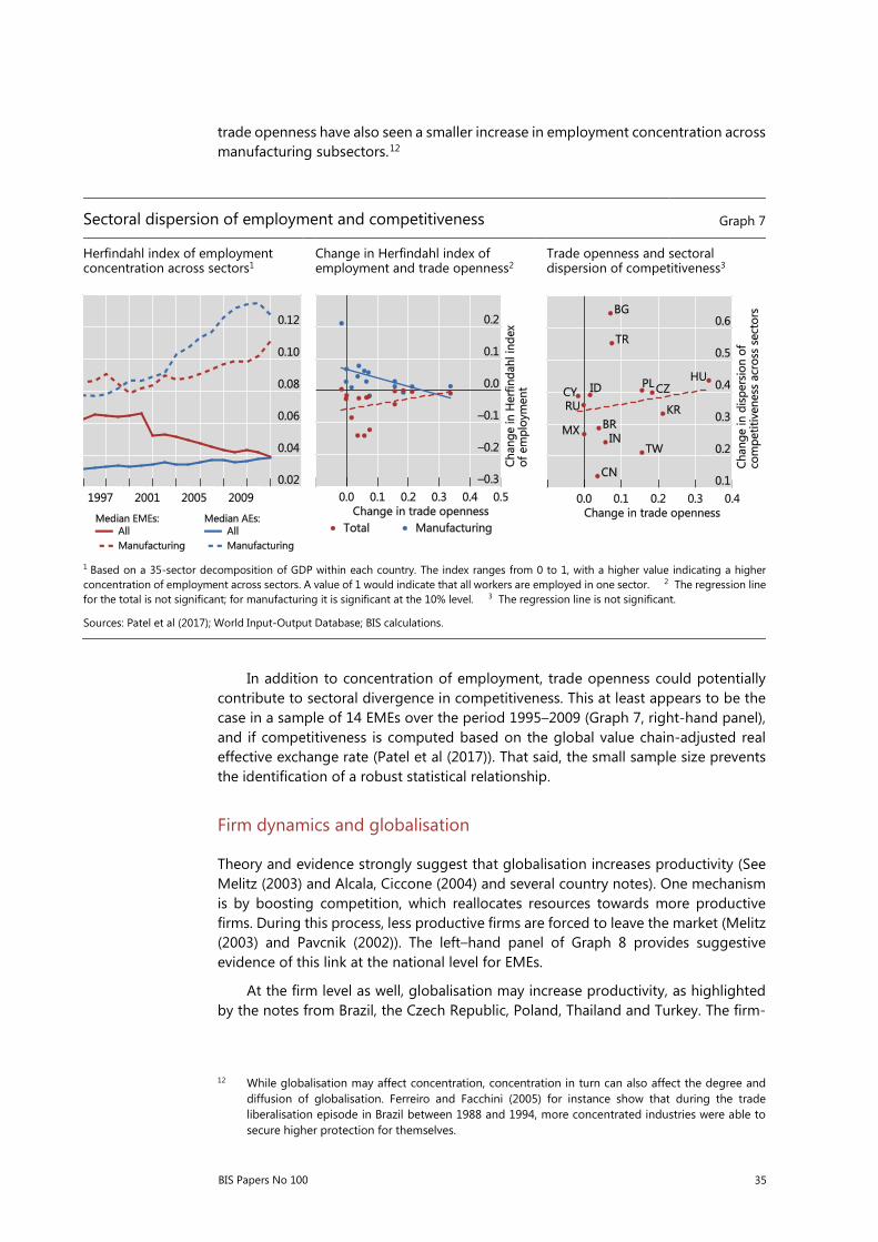
BIS Papers No 100 35
trade openness have also seen a smaller increase in employment concentration across manufacturing subsectors.12
Sectoral dispersion of employment and competitiveness Graph 7
Herfindahl index of employment concentration across sectors1
Change in Herfindahl index of employment and trade openness2
Trade openness and sectoral dispersion of competitiveness3
1 Based on a 35-sector decomposition of GDP within each country. The index ranges from 0 to 1, with a higher value indicating a higher concentration of employment across sectors. A value of 1 would indicate that all workers are employed in one sector. 2 The regression line for the total is not significant; for manufacturing it is significant at the 10% level. 3 The regression line is not significant.
Sources: Patel et al (2017); World Input-Output Database; BIS calculations.
In addition to concentration of employment, trade openness could potentially contribute to sectoral divergence in competitiveness. This at least appears to be the case in a sample of 14 EMEs over the period 1995–2009 (Graph 7, right-hand panel), and if competitiveness is computed based on the global value chain-adjusted real effective exchange rate (Patel et al (2017)). That said, the small sample size prevents the identification of a robust statistical relationship.
Firm dynamics and globalisation
Theory and evidence strongly suggest that globalisation increases productivity (See Melitz (2003) and Alcala, Ciccone (2004) and several country notes). One mechanism is by boosting competition, which reallocates resources towards more productive firms. During this process, less productive firms are forced to leave the market (Melitz (2003) and Pavcnik (2002)). The left–hand panel of Graph 8 provides suggestive evidence of this link at the national level for EMEs.
At the firm level as well, globalisation may increase productivity, as highlighted by the notes from Brazil, the Czech Republic, Poland, Thailand and Turkey. The firm-
12 While globalisation may affect concentration, concentration in turn can also affect the degree and
diffusion of globalisation. Ferreiro and Facchini (2005) for instance show that during the trade liberalisation episode in Brazil between 1988 and 1994, more concentrated industries were able to secure higher protection for themselves.

36 BIS Papers No 100
level analysis in Polish note shows that internationalised firms perform better than the rest, through both exporting and foreign ownership. The note by the Czech Republic undertakes a meta-analysis and concludes that a 10-percentage point increase in foreign presence is likely to lift the productivity of domestic firms by 11%. The effect is even larger for joint ventures, reaching 19%.
As a downside risk, globalisation may increase firm size concentration, benefiting larger firms at the expense of smaller ones.13 This is in part because access to a larger market allows firms to benefit from economies of both scale and scope, as offshoring and allocating production in multiple locations increases productivity. This, in turn, manifests itself in lower prices, increasing quality and product diversification (Schwörer (2013) and Constantinescu et al (2017)). While good for consumers, the transition may be painful for many smaller firms and their employees. Furthermore, in the long term, greater firm concentration may even harm productivity and growth by decreasing incentives for firms to invest due to lack of competition (Gutierrez and Philippon (2017)).
However, available data do not suggest a stark increase in firm size concentration.14 For example, while the share of employment in small and medium-sized enterprises (SMEs) decreased in EMEs in Latin America and Europe from the 1990s to the early 2000s, it increased post-GFC (Graph 8, second panel).15 Moreover, the SME share of employment share has been increasing in Asia-Pacific EMEs since the 1990s. And, other than in Mexico, the employment share of large firms has been declining in the EMEs for which data is available (Graph 9, left-hand panel). In Mexico, the share of employment in the top four firms (by employment) increased across sectors (Graph 8 third panel). In Poland, firm concentration, measured by Herfindahl indices, has been declining for employment but increasing for output (Graph 8, right-hand panel).
While firm inequality has not increased considerably in many EMEs, globalisation may have prevented a more equal size distribution. One way to analyse this channel is to examine whether sectors facing larger tariff declines experienced larger increases (or smaller declines) in the employment share of large firms.16 Graph 9 (centre and right-hand panels) shows that there is no such relationship in the data, suggesting that it is unlikely that globalisation has had a large impact.
13 Mechanisms outlined in Melitz (2003) would imply these dynamics. More highly productive firms are
likely to be bigger and to gain more from trade.
14 See ERIA Research Project Report (2013) for country-level evidence.
15 Employment is used as the measure of firm size.
16 Lower tariffs boost globalisation and may thus affect firm concentration.

BIS Papers No 100 37
Firm size concentration increases in some but not all EMEs Graph 8
Growth in trade and total factor productivity1
Per cent
SME employment share in EMEs4
Per cent
Top four firms’ employment share in Mexico
Per cent
Firm (industry sector) inequality in Poland
Herfindahl indices
1 Data for Algeria, Argentina, Brazil, Chile, China, Colombia, Hong Kong SAR, India, Indonesia, Israel, Korea, Malaysia, Mexico, Peru, the Philippines, Saudi Arabia, Singapore, South Africa, Thailand and Turkey. 2 Trade (exports + imports) as a percentage of GDP. 3 Indexed TFP with respect to 1979. 4 Simple averages across countries and years.
Sources: OECD, Structural Business Statistics; World Bank; The Conference Board; national data; BIS calculations.
Globalisation is unlikely to impact firm size concentration Graph 9
Share of employment by large firms1 Sectoral changes in tariffs and in large firms’ employment share2
Sectoral changes in tariffs and in large firms’ employment share2
1 Share of employees employed by firms with more than 250 employees as a percentage of total employment; simple averages of all sectors. The number of sectors differs across years and countries. 2 For each sector, change in the weighted average tariff and in the share of employees employed by firms with more than 250 employees (in percentage points). Depending on the sectors and country, the sample period could be a subset of the maximum sample, which runs from 1992 to 2009.
Sources: OECD, Structural Business Statistics; World Bank, World Development Indicators; World Bank, World Integrated Trade Solutions; BIS calculations.

38 BIS Papers No 100
3. Income and consumption inequality
Critics of globalisation have been vocal in singling out the phenomenon for the rise in (within-country) income inequality. Indeed, income inequality has worsened significantly in some EMEs and, probably more importantly, this deterioration is positively correlated with globalisation (Graph 10, first and second panels).17 At the same time, while the share of the population living below the poverty line has declined substantially, the bottom decile in the income distribution has been left behind compared with those enjoying an average income (Graph 10 third panel).18 The income trend of the growing middle class, which has a strong political voice, also plays a large part in determining sentiment towards globalisation, and consequently the leadership’s stance. That share has stalled, while that of the top 10% has surged in some EMEs (Graph 10, right-hand panel and Saez et al (2018)). At the global level, however, inequality has declined, as the proportion of the global population with annual incomes between $750 and $6,000 (PPP-adjusted) is growing rapidly (Lakner and Milanovic (2016)).19
Globalisation and income inequality are positively related Graph 10
Change in Gini coefficients1 Globalisation and Gini coefficients2, 3
Globalisation and low income2
Globalisation and high income2
1 Difference between the average coefficient before 1980 and between 2000 and 2015. 2 Trade openness is measured as imports plus exports divided by GDP. The changes are calculated over different years due to data availability. 3 The regression line is significant at the 5% level.
Sources: Lakner and Milanovic (2016); IMF, World Economic Outlook; BIS calculations.
One mechanism through which globalisation may increase inequality is through its impact on compensation within different labour market segments. As part of a broader global trend, EMEs have, on average, seen a sharp rise in the compensation
17 For a set of Asian economies, Park (2017) finds that higher globalisation is correlated with higher
income inequality.
18 The note by Russia argues that, while globalisation has contributed to rising inequality, it has undoubtedly been a major force behind the reduction in poverty.
19 Lengthy time series data for wealth inequality are scarcer than those for income inequality. See Novokmet et al (2017) for the dynamics of wealth inequality in China, the Czech Republic, Hungary, Poland and Russia. See Alvaredo (2010) for the case of Argentina.
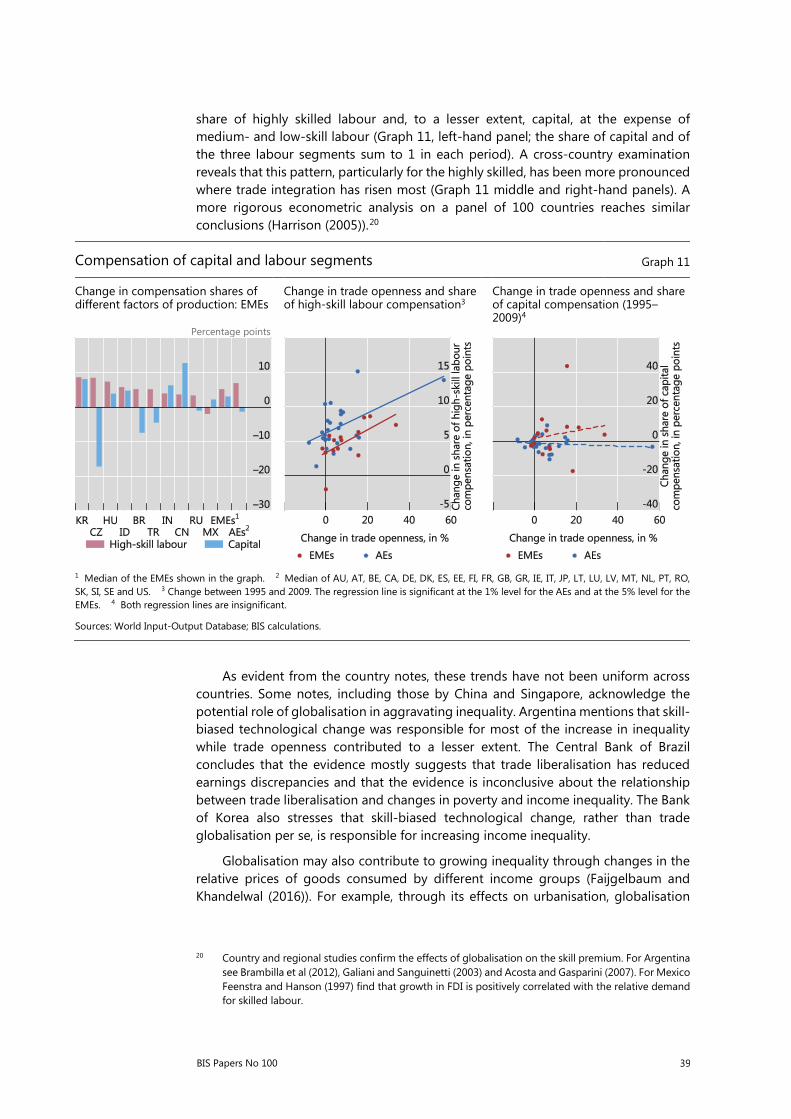
BIS Papers No 100 39
share of highly skilled labour and, to a lesser extent, capital, at the expense of medium- and low-skill labour (Graph 11, left-hand panel; the share of capital and of the three labour segments sum to 1 in each period). A cross-country examination reveals that this pattern, particularly for the highly skilled, has been more pronounced where trade integration has risen most (Graph 11 middle and right-hand panels). A more rigorous econometric analysis on a panel of 100 countries reaches similar conclusions (Harrison (2005)).20
As evident from the country notes, these trends have not been uniform across countries. Some notes, including those by China and Singapore, acknowledge the potential role of globalisation in aggravating inequality. Argentina mentions that skill-biased technological change was responsible for most of the increase in inequality while trade openness contributed to a lesser extent. The Central Bank of Brazil concludes that the evidence mostly suggests that trade liberalisation has reduced earnings discrepancies and that the evidence is inconclusive about the relationship between trade liberalisation and changes in poverty and income inequality. The Bank of Korea also stresses that skill-biased technological change, rather than trade globalisation per se, is responsible for increasing income inequality.
Globalisation may also contribute to growing inequality through changes in the relative prices of goods consumed by different income groups (Faijgelbaum and Khandelwal (2016)). For example, through its effects on urbanisation, globalisation
20 Country and regional studies confirm the effects of globalisation on the skill premium. For Argentina
see Brambilla et al (2012), Galiani and Sanguinetti (2003) and Acosta and Gasparini (2007). For Mexico Feenstra and Hanson (1997) find that growth in FDI is positively correlated with the relative demand for skilled labour.
Compensation of capital and labour segments Graph 11
Change in compensation shares of different factors of production: EMEs
Change in trade openness and share of high-skill labour compensation3
Change in trade openness and share of capital compensation (1995–2009)4
Percentage points
1 Median of the EMEs shown in the graph. 2 Median of AU, AT, BE, CA, DE, DK, ES, EE, FI, FR, GB, GR, IE, IT, JP, LT, LU, LV, MT, NL, PT, RO, SK, SI, SE and US. 3 Change between 1995 and 2009. The regression line is significant at the 1% level for the AEs and at the 5% level for the EMEs. 4 Both regression lines are insignificant.
Sources: World Input-Output Database; BIS calculations.

40 BIS Papers No 100
has probably boosted urban house prices, especially where land is scarce (Graph 12, left-hand panel). UBS city-level data reveal that the cost of housing relative to income has risen (Graph 12, second panel). Although it does embody a strong cyclical component likely linked to the financial cycle, a comparison with automobile affordability highlights a marked upward trend.21 Perhaps more importantly, food prices have increased more than those for other goods, not least due to the shift of resources towards manufacturing and services, without compensating efficiency gains in agriculture (Graph 12, third and fourth panels).22 As low-income individuals and countries spend a larger share of income on housing and food than higher income ones, these changes may have disproportionately affected the welfare of lower-income groups. For example, Akçelik (2016) finds that in Turkey the inflation differential between the first and fifth quantiles of the income distribution averaged 0.65 percentage points during 2004–15, due mainly to higher food price inflation. Moreover, this difference rises with income levels. And IMF (2008) finds that poverty tends to increase with higher food prices.
Price dynamics differ across sectors and goods Graph 12
The rise of urbanisation and house prices1
Cost of housing and automobiles relative to income2
Annual food price inflation in excess of CPI3
Agriculture PPI has been growing faster than manufacturing PPI3
Index Per cent Per cent
1 Included countries: AE, AR, BR, CL, CN, CO, CZ, HK, HU, ID, IN, KR, MX, MY, PE, PH, PL, RU, SG, TH, TR and ZA (see footnote in Graph 2 for country codes). The regression line becomes insignificant when heteroscedasticity is controlled for. 2 Average prices are divided by average income. Cost at the initial year is normalised to one. Cities included Abu Dhabi, Bangkok, Beijing, Bogotá, Budapest, Buenos Aires, Dubai, Hong Kong, Istanbul, Jakarta, Jeddah, Johannesburg, Kuala Lumpur, Lima, Manila, Mexico City, Moscow, Mumbai, New Delhi, Prague, Rio de Janeiro, São Paulo, Santiago de Chile, Seoul, Shanghai and Warsaw. 3 Average annual inflation differential for the period for which data are available. Periods with higher than 20% inflation are excluded.
Sources: World Bank; Datastream; UBS; national data; BIS calculations.
Higher mobility in the income distribution could, in principle, increase tolerance for income inequality. Higher mobility offers individuals greater opportunities to achieve higher incomes, thereby increasing the chances that a given income
21 See Wang et al (2015) for a more formal analysis. 22 Although trade in agricultural goods may have put downward pressure on food prices (as in other
sectors), this was probably has not been large enough to offset other forces.

BIS Papers No 100 41
distribution is perceived as fair. However, the data suggest that higher income inequality tends to be associated with greater inequality of opportunity and lower intergenerational economic mobility (Krueger (2012)). One reason could be that income inequality reduces opportunities for children from lower-income backgrounds to obtain education and skills (see also World Bank (2018)). This leads to a vicious circle in which higher income inequality and lower income mobility reinforce one another.
4. Effects of migration on human capital in EMEs
There are concerns that outward migration, particularly that of highly skilled workers, constitutes a “brain drain” for EMEs. Indeed, the migration of highly skilled workers, defined as those with a tertiary degree, has increased more rapidly than that of the less skilled. Growing by 170% between 1980 and 2010, the share of highly skilled workers in total immigrants to advanced economies rose by close to 20 percentage points to almost 40% (Graph 13, left-hand panel). This was at the expense of the share of low-skill workers (with little education), while that of medium-skill ones (with secondary level education) stayed largely unchanged.
EMEs have contributed significantly to the migration flows of skilled workers (Graph 13, right-hand panel). The number of highly skilled immigrants from major EMEs to advanced economies tripled between 1980 and 2010. Workers in the high-skill segment tend to emigrate at a higher rate than those in lower skill segments. The proportion of highly skilled emigrants in the highly skilled population averaged 13.5% in 2010 among EMEs (Graph 13, right-hand panel). The corresponding number was much lower for the low-skill segment. This pattern is also true at the country level (Graph 14, darker colours indicate more high (low) skill emigrants as a proportion of population with high (low) skill levels).
Some EMEs have seen particularly large shares of highly skilled workers emigrating. The note by the central bank of the Philippines points to a shift in the profile of Filipino migrants from mostly medium- or low-skill workers in the 1970s to professional workers in the 1990s as well as services and production (manufacturing and construction) workers from the 2000s.
Such a loss of skilled labour may cause skill shortages in some sectors. Obvious examples include occupations in the health and financial sectors, which are staffed by a higher portion of highly educated professionals. On a larger scale, such losses can dampen productivity and long-term growth prospects. In their note, the central bank of the Philippines identified emigration and the associated labour shortage as a major policy concern.
Yet, a few factors can dampen or even more than offset this negative impact. Remittances are disproportionally spent on education and health (Ratha and Mohapatra (2011); Cardona-Sosa and Medina (2006)). This not only gives emigrants’ families greater access to education, but also creates demand for better education and helps retain staff. Many migrants travel between their home and host countries, helping “brain circulation” by facilitating information and knowledge-sharing. In the longer run, migrants returning to their home countries with skills learned abroad can help improve domestic technology, management and institutions, leading to “brain gains”.

42 BIS Papers No 100
Higher outward migration from EMEs Graph 13
Immigration to advanced economies by skill level EME emigrants by skill levels in origin countries Per cent millions Per cent
1 EME high/low skill emigrants as percentage of EME high/low skill population. 2 EME emigrants as percentage of EME population.
Sources: OECD; United Nations.
In addition to the impact on source countries, there are several costs and benefits
of migration for recipient EME countries. For instance, as pointed out in the Bank of Korea’s note, migration has been important in helping the economy cope with a shrinking working-age population. Even so, the large inflow of mostly low-skill migrants has led to a rising wage gap, which is now an important policy concern. The note by Russia highlights how the adjustment of foreign migrant flows in response to the strength of the Russian economy acts as a cushioning device and reduces volatility of wages and employment for domestic workers.
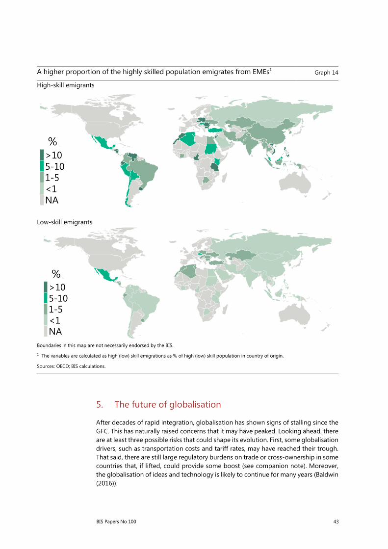
BIS Papers No 100 43
A higher proportion of the highly skilled population emigrates from EMEs1 Graph 14
High-skill emigrants
Low-skill emigrants
Boundaries in this map are not necessarily endorsed by the BIS.
1 The variables are calculated as high (low) skill emigrations as % of high (low) skill population in country of origin.
Sources: OECD; BIS calculations.
5. The future of globalisation
After decades of rapid integration, globalisation has shown signs of stalling since the GFC. This has naturally raised concerns that it may have peaked. Looking ahead, there are at least three possible risks that could shape its evolution. First, some globalisation drivers, such as transportation costs and tariff rates, may have reached their trough. That said, there are still large regulatory burdens on trade or cross-ownership in some countries that, if lifted, could provide some boost (see companion note). Moreover, the globalisation of ideas and technology is likely to continue for many years (Baldwin (2016)).
>105-101-5<1NA
%
>105-101-5<1NA
%

44 BIS Papers No 100
Second, technological developments, specifically the rise of automation, could change the nature of globalisation and curb trade. In contrast to earlier periods where technology was a driver of globalisation, advances in automation may soon enable machines to replace many jobs in EMEs, and hence reverse globalisation. Indeed, industries that have played an important role in the diversification of global trade and GVCs are increasingly relying on automated production (Graph 15, left-hand and centre panels). Moreover, the share of employment susceptible to automation in EMEs exceeds one third of the total employment in many cases, and in some countries it forms the greater part (Graph 15, right-hand panel). For example, in the case of Argentina, the country note cites a study by the ministry of finance that puts the probability that a job could be automated at 24–77%, depending on the sector.
Automation poses a risk for jobs Graph 15
New installations of industrial robots worldwide by industry, 2016
Sales of industrial robots worldwide
Estimated share of employment susceptible to automation1
Thousands Thousands Per cent
1 The values account for the slower pace of technology adoption in poorer countries, using the adoption lag of earlier technologies (Comin and Mestieri (2013)).
Source: International Federation of Robotics; World Bank, World Development Report 2016.
Third, a growing public perception that the losses from globalisation are bigger
than the gains could induce a backlash. Indeed, negative attitudes towards it have been gaining ground in EMEs (Graph 16, right-hand panel), although GDP growth coincides with a positive perception of globalisation (Graph 16, left-hand panel). This sentiment is also evident in the public perception of globalisation’s effect in reducing prices and creating jobs (Graph 17). Additionally, despite the potential benefits of FDI, public attitudes towards it (in both EMEs and AEs) are not as positive as one might expect (Graph 18). The way FDI is carried out matters dramatically for perception. For instance, the public may react more negatively to foreign firms’ acquisitions of domestic firms than to newly established factories.

BIS Papers No 100 45
Attitudes towards globalisation have worsened Graph 16
Weaker growth, worse attitudes Attitudes generally deteriorated between 2002 and 20141
Percentage points
1 Attitude in a year is calculated as the percentage of the people indicating globalisation is good minus the number that indicates globalisation is bad.
Sources: The Economist; Pew Research Center, Global Attitudes Survey; YouGov; World Bank; BIS calculations.
The public sees globalisation as creating jobs but not as lowering relative prices
In percent Graph 17
Does globalisation lead to lower prices? Does globalisation lead to job creation or job losses?
Sources: Pew Research Center, Global Attitudes Survey; BIS calculations.

46 BIS Papers No 100
Public attitudes towards FDI are not uniformly positive1
In percentage points Graph 18
Towards foreign acquisitions of domestic companies
Towards foreign companies building new factories
1 Attitude in a year is calculated as the percentage of the people indicating the specific aspect of globalisation is good minus that indicating it is bad.
Sources: Pew Research Center, Global Attitudes Survey; BIS calculations.
Clearly, inward-looking policies have attracted more advocates since the GFC. But, if the historical experience of some Latin American countries provides any guide, cutting oneself off from globalisation can be harmful.23 The success of such policies is even less likely today, given much more complex and advanced technologies and a more marked division of labour.
The remainder of this section sketches possible policy options. For the most part, policies that can best deal with globalisation are structural in nature, and are mostly outside the realm of traditional central banking. Yet, central banks may have a valuable role to play in communicating the benefits of globalisation and contributing to macroeconomic stability.
Going forward with globalisation
Despite a substantial easing of the restrictions on the cross-border movement of goods, services and people, numerous restrictions still remain in place in many EMEs. Tariffs are high and non-tariff measures (NTM) widespread in several countries. Similarly, as highlighted in Note 1, trade in services still faces major regulatory restrictions. In addition, the level of complexity and costs related to border and documentary compliance could be simplified and reduced considerably in some countries. For example, allowing electronic submission and processing of customs information can save both time and money. The same is true of streamlining administrative processes and greater logistic efficiency. However, most EMEs are still lagging in their efforts to facilitate trade (Graph 19).
23 See, for example, Hopenhayn and Neumeyer (2004) for Argentina’s experience.

BIS Papers No 100 47
Implementation status of trade facilitation measures
UN Global Survey on Trade Facilitation and Paperless Trade Implementation, 20171 Graph 19
Per cent
1 Implementation status is based on 47 measures related to the WTO's Trade Facilitation Agreement (TFA), paperless trade, and inclusive development. Higher values mean higher trade facilitation.
Source: United Nations, Global Survey on Trade Facilitation and Paperless Trade Implementation 2017.
Dealing with de-globalisation risks
Responding to worsening public attitudes towards globalisation is another area of concern for policymakers. For instance, the survey responses shown in Graph 17 reveal that for most of the countries fewer than half of the respondents think that trade puts downward pressure on prices, even though most of the related literature suggests that this is the case (IMF (2006) and Pain et al (2008)). Better communication might help improve these attitudes, and central banks, given their price mandates, may have a particularly important role to play.
Could EMEs do anything about the rising support for inward-looking policies in advanced economies? Diversifying exports (both across sectors and destinations) could help address threats from greater protectionism, as pointed out in the note by the central bank of Malaysia.
The increasing automation of production also raises challenges.24 It may reduce EMEs’ labour cost advantage and, therefore, reverse some of the production offshored by AEs. Besides, not only the AEs, but also the EMEs themselves are increasingly using these technologies, which may reduce the demand for labour. Indeed, the types of job that are more prevalent in EMEs are more susceptible to automation, as suggested in Graph 15.
24 One of the three main issues earmarked as key priorities in the Argentine G20 presidency is the
“Future of work”. This focuses on policies to harness technological innovation and mitigate its likely disruptive effects on labour markets.

48 BIS Papers No 100
Policies to address an uneven distribution of the benefits
While globalisation has probably boosted overall welfare in EMEs, the benefits have typically been unevenly spread. The major challenge for policymakers is therefore how to reduce adjustment costs and narrow the gap between winners and losers.
Policies that facilitate the reallocation of labour and capital across sectors are one option. These would help avoid pockets of unemployment and, over time, facilitate a more productive use of resources. Making the labour and product markets sufficiently flexible, as well as retraining programmes, could play a useful role. In addition, trade agreements could be introduced in a gradual and phased manner to minimise the costs of trade liberalisation.25 A case in point is the Singaporean government’s move to promote job matching and re-skilling of mid-career professionals (see note).
But even if full employment is ensured, income and wealth inequality remain a major challenge. Hence a role for redistributive policies.26 These, in turn, call for adequate social security and welfare systems.27 Relevant policies include unemployment insurance, food subsidies and laws to promote efficient labour mobility and severance payments. One such example, as pointed out by the central bank of Malaysia, is the Malaysia Outplacement Centre (1MOC) established by the government in 2016 to help displaced workers find new jobs. Thus far, the centre has placed 2,400 workers. As the Monetary Authority of Singapore points out, the scope for redistributive policies is not limited to households and individuals. Indeed, the government has provided time-bound investment support as well as targeted relief to firms heavily affected by structural change. Political hurdles aside, the main roadblock for many EMEs is the lack of a sizeable and stable tax base. Hence the role for policies that enhance the tax system’s efficiency and compliance rate.
More generally, the challenge for policymakers is to harness globalisation to support robust and sustainable long-term growth. This raises the question of the appropriate growth model. For instance, manufacturing and commodity exports have been instrumental for many countries in boosting growth. But looking ahead, this growth model may come under pressure from the shift in world demand away from tradable manufactured goods to non-tradable services.
In EMEs, globalisation has gone hand in hand with urbanisation, ageing populations and growing environmental risks. Governments have a menu of policy options here. For instance, they can ease adjustment by devoting adequate resources to urban planning and infrastructure. They may also invest in rural infrastructure to increase productivity there, as the contribution from the People’s Bank of China points out. However, the fact that the benefits materialise only over horizons longer than the typical political cycle complicates the challenge.
Many of these challenges are best addressed at the national level, tailoring policy responses to specific needs. Nevertheless, there are also issues such as climate
25 As pointed out by the country note by Malaysia, the ASEAN free trade agreement (AFTA) is a
prominent example of this approach. It also includes a “Temporary Exclusion List”, a “Sensitive List” and a “General Exception List” to safeguard the interests of individual countries.
26 Naturally, such policies cannot substitute for having a job: subjective well-being depends not only on income, but also on how that income is earned (eg Helliwell et al (2017) and Ohtake (2012)).
27 Several country notes (including those by the Philippines and Brazil) identified strengthening social security systems as an important part of the policy response.

BIS Papers No 100 49
change and cyber-security where the scope for international cooperation is naturally greater.
Although central banks do not have direct responsibility for the policies just discussed, they can have a role to play. One is simply voicing views about the right policies for governments to follow: the consequences for central banks would be of first-order significance. The scope for this will depend on country-specific circumstances and institutional setups. Central banks may also need to consider how far to take into account in their policy decisions some of the distributional consequences of globalisation across sectors or the population. They may need a better understanding of the implications of globalisation for economic performance and inflation. Likewise, the growing importance of the external dimension naturally puts a premium on the potential role of FX regimes and policies that help address external shocks. For instance, not surprisingly, the use of FX intervention has been on the rise in EMEs (Domanski et al (2016)).28 Similarly, several contributions, including the ones from the Bank of Korea, the Hong Kong Monetary Authority and the People’s Bank of China, mention the potential role of macroprudential frameworks and capital flow management measures in helping to insulate the domestic economy from foreign shocks. As pointed out by the country notes of Brazil and the Philippines, central banks in EMEs can also contribute to the efficacy of the overall policy response to globalisation by promoting financial inclusion.
Greater policy challenges lie ahead if protectionism prevails and globalisation reverses. In that case, benefits will likely be reversed: growth may slow, inflation may rise, GVCs may be disrupted and jobs destroyed. While tighter regional integration may be an option to alleviate the costs, it may not be enough.
28 Several country notes, including Malaysia’s, corroborate this view.

50 BIS Papers No 100
References
Acosta, P and L Gasparini (2007): “Capital accumulation, trade liberalization, and rising wage inequality: the case of Argentina”, Economic Development and Cultural Change, vol 55.
Akçelik, F (2016): Income groups and inflation in Turkey, master’s thesis.
Alcalá, F and A Ciccone (2004): “Trade and productivity”, Quarterly Journal of Economics, vol 119, no 2, pp 613–46.
Alvaredo, A (2010): “The rich in Argentina over the twentieth century, 1932–2004”, Top Incomes: A Global Perspective, pp 253–98.
Amiti, M (1999): “Specialization patterns in Europe”, Weltwirtschaftliches Archiv (Review of World Economics), vol 135, no 4, pp 573–93.
Antràs, P, A De Gortari and O Itskhoki (2016): ”Globalization, inequality and welfare”, NBER Working Papers, no 22676.
Auer, R, C Borio and A Filardo (2017): “The globalisation of inflation: the growing importance of global value chains“, BIS Working Papers, no 602.
Baldwin, R (2016): The great convergence, Harvard University Press.
Bank for International Settlements (2017): 87th Annual Report.
Beaton, K, S Cerovic, M Galdamez, M Hadzi-Vaskov, F Loyola, Z Koczan, B Lissovolik, J Martijn, Y Ustyugova and J Wong (2017): “Migration and remittances in Latin America and the Caribbean: engines of growth and macroeconomic stabilizers?”, IMF Working Papers, no 17/144.
Black, S and E Brainerd (2004): “Importing equality? The impact of globalization on gender discrimination”, Industrial and Labor Review, vol 57, no 4.
Brambilla, I, D Lederman and G Porto (2012): “Exports, export destinations and skills,” American Economic Review, vol 102, no 7.
Cavallo, E and J Frankel (2008): “Does openness to trade make countries more vulnerable to sudden stops, or less? Using gravity to establish causality“, Journal of International Money and Finance, vol 27, no 8, pp 1430–52.
Cardona-Sosa, L and C Medina (2006): “Migration as a safety net and effects of remittances on household consumption: the case of Colombia”, Borradores De Economia, Bank of the Republic, Colombia.
Comin, D and M Mestieri (2013): “If technology has arrived everywhere, why has income diverged?”, NBER Working Paper, no 19010.
Constantinescu, C, A Mattoo and M Ruta (2017): “Does vertical specialization increase productivity?”, Policy Research Working Paper, no 7978, World Bank.
Czaika, M and H de Haas (2016): “The effects of visas on migration processes”, International Migration Review, vol 51, no 4, pp 893–926.
Domanski, D, E Kohlscheen, and R Moreno (2016): “Foreign exchange market intervention in EMEs: what has changed?”, BIS Quarterly Review, September.
Dreher, A (2006): “Does globalization affect growth? Evidence from a new index of globalization”, Applied Economics, vol 38, no 10.
BIS Papers No 100 51
ERIA Research Project Report (2013): “Globalization and performance of small and large firms“.
Faijgelbaum, P and A Khandelwal (2016): “Measuring the unequal gains from trade”, Quarterly Journal of Economics, vol 131.
Feenstra, R and G Hanson (1997): “Foreign direct investment and relative wages: evidence from Mexico’s maquiladoras”, Journal of International Economics, vol 42, pp 371–93.
Ferreiro, P and G Facchini (2005): “Trade liberalization and industrial concentration: evidence from Brazil”, the Quarterly Review of Economics and Finance, vol 45.
Frankel, J and A Rose (1998): “The endogeneity of the optimum currency area criteria”, The Economic Journal, vol 108, no 449, pp 1009–25.
Galiani, S and P Sanguinetti (2003): “The impact of trade liberalization on wage inequality: evidence from Argentina”, Journal of Development Economics, vol 72, no 2.
Giordano, P and K Li (2012): “An updated assessment of the trade and poverty nexus in Latin America”, IDB Working Paper Series, IDB-WP-383, Washington DC.
Gopinath, G, S Kalemli-Ozcan, L Karabarbounis and C Villegas-Sanchez (2017): “Capital allocation and productivity in South Europe”, NBER Working Paper, no 21453.
Gutierrez, G and T Philippon (2017): ”Declining competition and investment in the US”, manuscript.
Harrison, A (2005): “Has globalization eroded labor’s share? Some cross-country evidence”, MPRA Paper, no 39649.
Helliwell, J, H Huang and S Wang (2017): “The social foundations of world happiness”, World Happiness Report 2017, Chapter 8.
Hopenhayn, H and P Neumeyer (2004): “Explaining Argentina’s great depression of 1975–1990” in E Fernandez-Arias, R Manuelli and J Blyde (eds), Sources of growth in Latin America. What is missing?, Inter-American Development Bank.
IMF (2006): World Economic Outlook, April.
——— (2008): Food and fuel prices – recent developments, macroeconomic impact, and policy responses, 30 June.
Kose, A, C Otrok and E Prasad (2012): “Global business cycles: Convergence or decoupling”, International Economic Review, vol 53, no 2, pp 511–38.
Krueger, A (2012): “The rise and consequences of inequality in the United States”, speech at the Center for American Progress, Washington DC, 12 January.
Kuznets, S (1971): Prize Lecture: “Modern economic growth: findings and reflections”, Stockholm: The Nobel Prize.
Lakner, C and B Milanovic (2016): “Global income distribution: from the fall of the Berlin wall to the great recession”, World Bank Economic Review, vol 30, no 2.
Lee, J and J Pyun (2008): “Does trade integration contribute to peace”, ADB Working Paper Series on Regional Economic Integration, no 24, December.
Melitz, M (2003): “The impact of trade on intra-industry reallocations and aggregate industry productivity”, Econometrica, vol 71, no 6, pp 1695–725.

52 BIS Papers No 100
Novokmet, F, T Piketty and G Zucman (2017): “From Soviets to oligarchs: Inequality and property in Russia, 1905–2016”, World Income Database, Working Paper Series, no 2017/09.
Ohtake, F (2012): “Unemployment and happiness”, Japan Labor Review, vol 9, no 2, Spring.
Pain, N, I Koske and M Sole (2008): “Globalisation and OECD consumer price inflation”, OECD Economic Studies, no 44.
Park, K (2017): “Education, globalization and income inequality in Asia”, ADBI Working Paper Series, no 732.
Patel, N, Z Wang and S Wei (2017): “Global value chains and effective exchange rates at the country-sector level”, BIS Working Papers, no 637.
Pavnick, N (2002): “Trade liberalization, exit, and productivity improvements: evidence from Chilean plants”, Review of Economic Studies, vol 69, no 1, January, pp 245–76.
Ratha, D and S Mohapatra (2011): “Preliminary estimates of diaspora savings”, Migration and Development Brief, no 14, World Bank.
Rodrik, D (2008): “The disappointments of financial globalization”, in Bank of Thailand, Financial Globalization and Emerging Market Economies, Proceedings of an International Symposium, Bangkok, November.
——— (2017): “Populism and the economics of globalization”, NBER Working Paper, no 23559.
Rutherford, T and D Tarr (2005): “Russia’s WTO accession: what are the macroeconomic, sector, labor market and household effects?”, in G Navaretti (ed), Handbook of Trade Policy and WTO Accession for Development in Russia and the CIS, World Bank.
Saez, E, F Alvaredo, L Chancel and T Piketty (2018): World Inequality Report 2018.
Schwörer, T (2013): “Offshoring and labour market inequalities”, Kiel Working Paper, no 1877, Kiel Institute for the World Economy.
Wang, Z, C Wang and Q Zhang (2015): “Population ageing, urbanization and housing demand”, Journal of Service Science and Management, vol 8, no 4, pp 516–25.
World Bank (2018): Fair Progress?: Educational mobility around the world. Equity and development, Washington DC.

BIS Papers No 100 53
Appendix
A1. Herfindahl index of concentration of employment across sectors: individual country plots
Graph A1 shows the evolution of the Herfindahl index of concentration for employment in the sample period 1995–2011. Countries are split into two groups (high and low) depending on the level of the index.
A2. Relationship Between trade and GDP growth
Trade and growth: Evidence from panel regressions
The dynamic panel regressions are based on a sample of 22 EMEs from 1979 to 2019. The dependent variable is the five-year moving average of per capita GDP growth, and the main independent variable of interest is the five-year moving average of growth in trade openness (lagged by one period), for which the corresponding row in the table is highlighted in bold. Column 1 uses a pooled estimator without any additional controls; it shows that trade openness boosts growth, with an elasticity of 0.03. Column 2 adds additional controls, including time fixed effects, and is based on a random-effects estimator. The positive relationship between trade openness and growth still survives, although it is statistically less robust (significant only at the 10% level). Column 3 shows the results using a fixed effects GMM estimator. While still positive, the coefficient is no longer statistically significant.
Overall, these results suggest that there is a positive relationship between growth and trade openness. However, the relationship ceases to be statistically significant once country fixed effects are included, indicating that the cross-country variation in these variables is insufficient to uncover a robust link.
Herfindahl index of concentration in employment across sectors Graph A1
High Herfindahl index Low Herfindahl index
Sources: World Input-Output Database; BIS calculations.
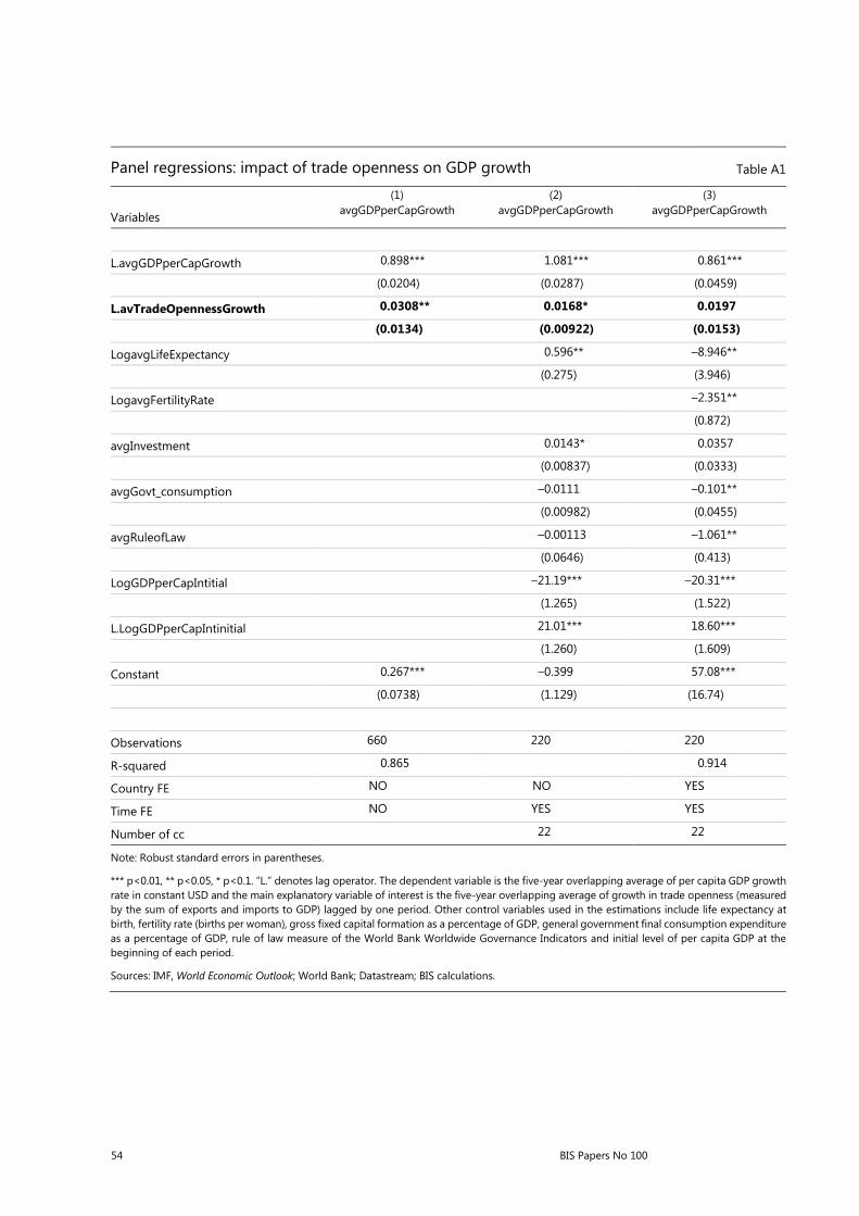
54 BIS Papers No 100
Panel regressions: impact of trade openness on GDP growth Table A1
Variables
(1) avgGDPperCapGrowth
(2) avgGDPperCapGrowth
(3) avgGDPperCapGrowth
L.avgGDPperCapGrowth 0.898*** 1.081*** 0.861***
(0.0204) (0.0287) (0.0459)
L.avTradeOpennessGrowth 0.0308** 0.0168* 0.0197
(0.0134) (0.00922) (0.0153)
LogavgLifeExpectancy 0.596** –8.946**
(0.275) (3.946)
LogavgFertilityRate –2.351**
(0.872)
avgInvestment 0.0143* 0.0357
(0.00837) (0.0333)
avgGovt_consumption –0.0111 –0.101**
(0.00982) (0.0455)
avgRuleofLaw –0.00113 –1.061**
(0.0646) (0.413)
LogGDPperCapIntitial –21.19*** –20.31***
(1.265) (1.522)
L.LogGDPperCapIntinitial 21.01*** 18.60***
(1.260) (1.609)
Constant 0.267*** –0.399 57.08***
(0.0738) (1.129) (16.74)
Observations 660 220 220
R-squared 0.865 0.914
Country FE NO NO YES
Time FE NO YES YES
Number of cc 22 22
Note: Robust standard errors in parentheses.
*** p<0.01, ** p<0.05, * p<0.1. “L.” denotes lag operator. The dependent variable is the five-year overlapping average of per capita GDP growth rate in constant USD and the main explanatory variable of interest is the five-year overlapping average of growth in trade openness (measured by the sum of exports and imports to GDP) lagged by one period. Other control variables used in the estimations include life expectancy at birth, fertility rate (births per woman), gross fixed capital formation as a percentage of GDP, general government final consumption expenditure as a percentage of GDP, rule of law measure of the World Bank Worldwide Governance Indicators and initial level of per capita GDP at the beginning of each period.
Sources: IMF, World Economic Outlook; World Bank; Datastream; BIS calculations.

BIS Papers No 100 55
Trade, growth and convergence
In the last few decades, EMEs have grown faster than advanced economies, converging towards advanced economy income levels. At the same time, as documented above, EMEs have also witnessed large increases in trade openness, and this has had a mainly positive impact on growth. A natural question to ask is to what extent these two trends have interacted. In particular, what has been the contribution of trade openness in convergence?
Graph A2 attempts to uncover the role of trade openness in the process of convergence of per capita GDP levels, and shows that the evidence is not clear-cut in either direction. While countries with low initial per capita income have grown more in line with the convergence hypothesis (dots towards the bottom are bigger than dots towards the top), globalisation has not had an unambiguously positive impact on this relationship. In fact, for a given level of starting income, countries that have grown most have been the ones that have experienced moderate levels of increases in globalisation (between 20 and 30 on the x axis), while countries with very high and very low growth in globalisation have grown comparatively less.
Globalisation and convergence: mixed evidence1 Graph A2
1 The size of the dots represents the growth of the PPP-adjusted GDP per capita between 1980 and 2013. The change in the economic globalisation index is also measured between 1980 and 2013. For the Czech Republic and Russia, the data start in 1995 and 1990, respectively. The dashed vertical lines indicate low, medium and high change in globalisation.
Sources: IMF, World Economic Outlook; Angus Maddison Data; KOF Globalization Index; BIS calculations.

56 BIS Papers No 100

BIS Papers No 100 57
Globalisation, growth and inequality from an emerging economy perspective
Central Bank of Argentina
Abstract
As a complex phenomenon, globalisation needs to be analysed on several levels. We discuss three related issues from the perspective of Latin American economies: the relationship between globalisation and growth performance; the possible trade-offs between integration and inequality, and the roles played by trade and technology; and how technological change may alter work relationships as we know them. Globalisation is a positive overall force for growth, but its interaction with domestic policies is crucial in determining the actual outcome. Technological innovation can have a positive effect on employment, but there is evidence of adverse distributional consequences. The outcome remains largely open, depending on the policy response.
Keywords: economic growth, globalisation, income distribution, technological change.
JEL classification: O40, O33, D30.

58 BIS Papers No 100
Introduction
Policymakers everywhere face the challenge of reaping the benefits of higher real and financial integration into world markets while mitigating its costs. Globalisation is a complex phenomenon, which should be analysed on several levels. In this note, we touch on three related issues from the perspective of Latin American economies in general and Argentina in particular: (i) the relationship between globalisation and growth performance; (ii) the possible trade-offs between integration and inequality, and the roles played by trade and technology; and (iii) how technological change may alter work relationships as we know them.
Integration, growth and policies
Empirical work gives support to the notion that trade goes hand in hand with growth, while the relationship between growth and financial integration with world markets is somewhat less robust – owing in part to the fact that such integration, if untamed, can lead to financial crises. The general consensus is that both trade and financial openness are expected to increase GDP growth.
Evidence for Latin America generally supports the consensus, but calls for a nuanced view (Giordano and Li (2012)). Looking at 13 Latin American countries, Sachs and Warner (1995) find that open economies performed better than closed ones during 1970–1989. But there are mixed results within the sample: Argentina, Costa Rica, Ecuador, El Salvador, Guatemala and Uruguay were found to grow more after liberalisation measures, while the opposite holds for Brazil, Colombia, Mexico, Nicaragua and Paraguay. Such results were criticised for the measurement of openness and possible reverse causality (whether trade causes growth or the opposite). Rodríguez and Rodrik (2001) objected to the choice of openness indicators (as weak measures of trade barriers), and pointed out that trade liberalisation episodes were significantly correlated with other macro- and microeconomic reforms – such as opening to foreign direct investment and deregulating labour markets.
In turn, Estevadeordal and Taylor (2013) stress the importance of identifying the period of analysis, and the specific liberalising measures. Reviewing the periods both before and after what they call the GATT “Great Liberalisation,” they distinguish between liberalising and non-liberalising countries. They find that reducing tariffs on imported capital goods led to faster growth.
Incorporating complementary policies into the analysis, Bolaky and Freund (2004) find that trade opening promotes growth only in countries that are not excessively regulated (using a panel of 100 countries). Indeed, trade openness is linked to lower living standards in excessively regulated economies. In their view, highly regulated countries fail to generate growth because resources are prevented from flowing to the most productive activities.
The case of Argentina illustrates with utmost clarity the complexities involved in the trade-growth nexus: both factor endowments and their political economy consequences have to be factored in (Gerchunoff and Llach (2009)). Roughly speaking, three phases of growth performance can be identified in Argentina vis-à-vis the rest of the world (Graph 1): (i) convergence to advanced countries’ growth rates in 1870–1929, based on the country’s successful integration into world markets;
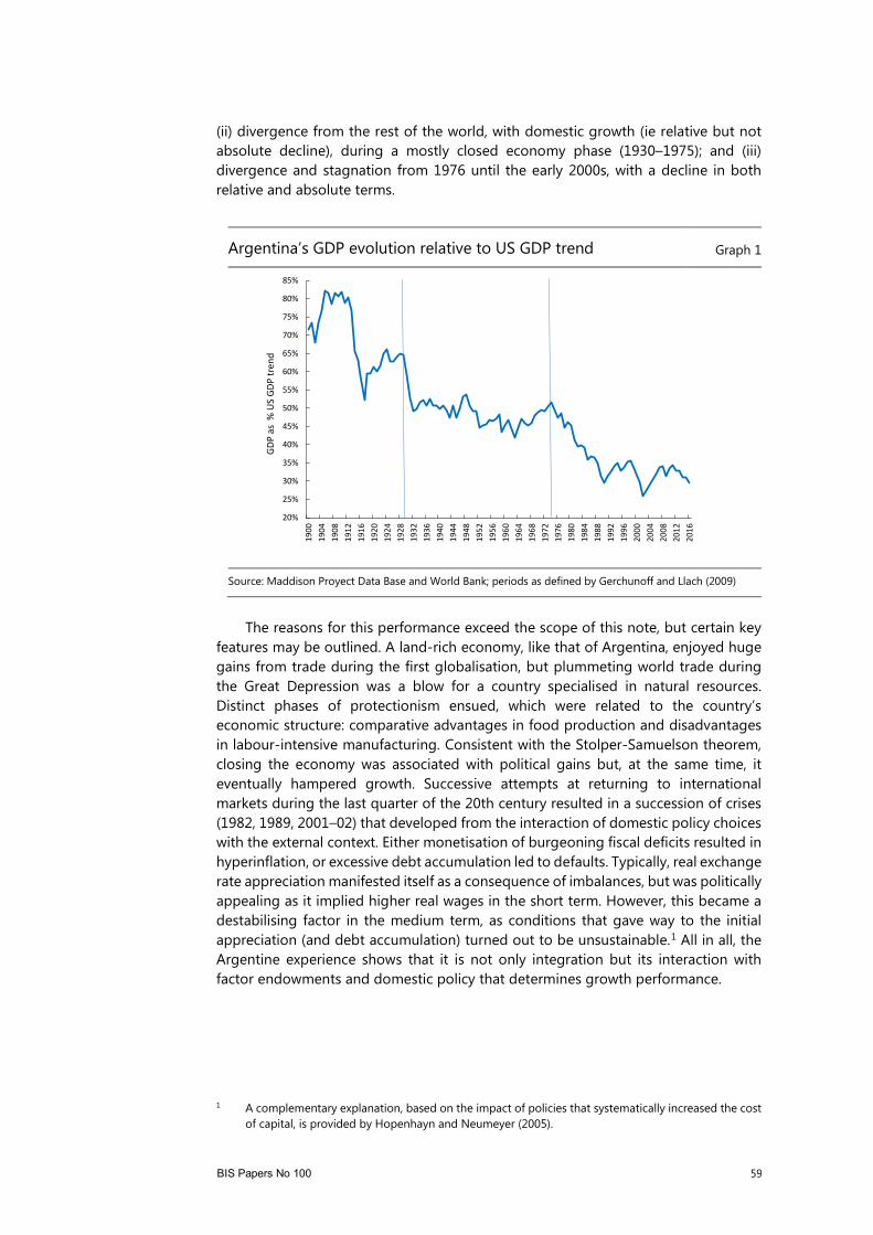
BIS Papers No 100 59
(ii) divergence from the rest of the world, with domestic growth (ie relative but not absolute decline), during a mostly closed economy phase (1930–1975); and (iii) divergence and stagnation from 1976 until the early 2000s, with a decline in both relative and absolute terms.
Argentina’s GDP evolution relative to US GDP trend Graph 1
Source: Maddison Proyect Data Base and World Bank; periods as defined by Gerchunoff and Llach (2009)
The reasons for this performance exceed the scope of this note, but certain key
features may be outlined. A land-rich economy, like that of Argentina, enjoyed huge gains from trade during the first globalisation, but plummeting world trade during the Great Depression was a blow for a country specialised in natural resources. Distinct phases of protectionism ensued, which were related to the country’s economic structure: comparative advantages in food production and disadvantages in labour-intensive manufacturing. Consistent with the Stolper-Samuelson theorem, closing the economy was associated with political gains but, at the same time, it eventually hampered growth. Successive attempts at returning to international markets during the last quarter of the 20th century resulted in a succession of crises (1982, 1989, 2001–02) that developed from the interaction of domestic policy choices with the external context. Either monetisation of burgeoning fiscal deficits resulted in hyperinflation, or excessive debt accumulation led to defaults. Typically, real exchange rate appreciation manifested itself as a consequence of imbalances, but was politically appealing as it implied higher real wages in the short term. However, this became a destabilising factor in the medium term, as conditions that gave way to the initial appreciation (and debt accumulation) turned out to be unsustainable.1 All in all, the Argentine experience shows that it is not only integration but its interaction with factor endowments and domestic policy that determines growth performance.
1 A complementary explanation, based on the impact of policies that systematically increased the cost
of capital, is provided by Hopenhayn and Neumeyer (2005).
20%
25%
30%
35%
40%
45%
50%
55%
60%
65%
70%
75%
80%
85%
1900
1904
1908
1912
1916
1920
1924
1928
1932
1936
1940
1944
1948
1952
1956
1960
1964
1968
1972
1976
1980
1984
1988
1992
1996
2000
2004
2008
2012
2016
GDP
as %
US
GDP
tren
d

60 BIS Papers No 100
Income inequality: is it trade or technology?
The preceding narrative illustrates certain trade-offs, of which perhaps the most salient is that gains from trade are not distributed evenly across the population – so that, roughly speaking, globalisation comes at the cost of income inequality.2 Or does it? The evidence in recent decades seems to be that higher trade and financial opening entail a small contribution to rising inequality, while the bulk of it seems to come from skill-biased technological change. For many developing economies, in which increasing trade means on many occasions reducing the price of hi-tech goods, it is very difficult to identify whether it is trade or technology that causes higher inequality.
The experience of Latin America in the last couple of decades is a case in point. Countries in the region put in place a suite of structural reforms from the 1990s onwards, including current and capital account liberalisation, deregulation and privatisation. These triggered foreign direct investment, and also reduced the price of capital. Most of the evidence suggests that these reforms were linked to a rise in earnings inequality, especially by curbing the relative demand for unskilled labour. In the case of Argentina, the evidence also points in the direction that skill-biased technological change was responsible for most of the increase in inequality (Acosta and Gasparini (2007)), while trade openness contributed to a lesser extent (Galiani and Sanguinetti (2003)).
A series of macroeconomic crises hit the region from the late 1990s, and this was associated with a spike in inequality. But the situation was reversed in the 2000s, with a very marked reduction in income inequality. This can be attributed to a number of factors, one of them being the very favourable terms of trade shock that the region experienced (Graph 2).
2 The conventional link is thought of as follows: trade between AEs and EMEs increases the returns to
AE skilled labour (but reduces that to unskilled labour, which is competing with EME unskilled labour) and increases returns for unskilled labour in EMEs.

BIS Papers No 100 61
Latin America: income inequality and terms of trade Graph 2
Source: Gasparini et al (2016), based on SEDLAC (CEDLAS and the World Bank) and WDI (World Bank).
The terms of trade of Latin American countries trended significantly higher during the first decade of the 2000s, leading to improved economic performance in the region. This translated into lower income inequality through at least two channels: increased labour demand and enhanced fiscal space. While growth in the 1990s was linked to higher demand for relatively highly skilled workers, the terms of trade shock went together with higher demand for labour across different sectors. In some economies, it actually increased demand for low-skilled workers; witness, for instance, the case of construction in many countries in the region.
Higher terms of trade also entailed a windfall for government revenues, which were partly allocated to increased social spending, including different types of workfare/conditional cash transfer programme, and enhanced pension and benefit coverage. At the same time, government regulation and policies such as higher minimum wages and a resurgent role for unions were all supportive of workers’ earnings.
That these redistributive effects were catalysed by higher terms of trade (TOT)3 is evident when the dynamics of commodity and non-commodity exporters are compared (Graph 3). The decline in Gini coefficients is notably higher in the former than in the latter.
3 This, of course, is not to deny the role of other equalising factors, including demography and
education.
44
46
48
50
52
54
56
60
70
80
90
100
110
120
1992
1993
1994
1995
1996
1997
1998
1999
2000
2001
2002
2003
2004
2005
2006
2007
2008
2009
2010
2011
2012
2013
2014
Inde
x, 2
010=
100
Terms of trade Gini coefficient (right hand side)
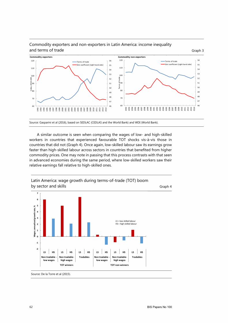
62 BIS Papers No 100
Commodity exporters and non-exporters in Latin America: income inequality and terms of trade Graph 3
Source: Gasparini et al (2016), based on SEDLAC (CEDLAS and the World Bank) and WDI (World Bank).
A similar outcome is seen when comparing the wages of low- and high-skilled
workers in countries that experienced favourable TOT shocks vis-à-vis those in countries that did not (Graph 4). Once again, low-skilled labour saw its earnings grow faster than high-skilled labour across sectors in countries that benefited from higher commodity prices. One may note in passing that this process contrasts with that seen in advanced economies during the same period, where low-skilled workers saw their relative earnings fall relative to high-skilled ones.
Latin America: wage growth during terms-of-trade (TOT) boom by sector and skills Graph 4
Source: De la Torre et al (2015).
Commodity exporters Commodity non-exporters
46
47
48
49
50
51
52
53
54
55
56
60
70
80
90
100
110
120
1992
1993
1994
1995
1996
1997
1998
1999
2000
2001
2002
2003
2004
2005
2006
2007
2008
2009
2010
2011
2012
2013
2014
Inde
x, 2
010=
100
Terms of tradeGini coefficient (right hand side)
46
47
48
49
50
51
52
53
54
55
56
60
70
80
90
100
110
120
1992
1993
1994
1995
1996
1997
1998
1999
2000
2001
2002
2003
2004
2005
2006
2007
2008
2009
2010
2011
2012
2013
2014
Ters
m o
f tra
de
Terms of tradeGini coefficient (right hand side)
-2
-1
0
1
2
3
4
5
6
7
LS HS LS HS LS HS LS HS LS HS LS HS
Non tradable -low wages
Non tradable-high wages
Tradables Non tradable -low wages
Non tradable-high wages
Tradables
TOT winners TOT non-winners
Wag
es: a
nnua
lized
grow
th ra
te, %
LS = low skilled labourHS = high skilled labour

BIS Papers No 100 63
During the 2010s, the improvement in income distribution indicators has apparently reached a plateau, in line with the reversal of terms of trade undergone by Latin America, and its lower growth performance. This poses multiple challenges to policymakers, as they now have to deal not only with slower growth but with potentially adverse distributional consequences.
To sum up, in Latin America in recent decades, integration with the world economy shows phases of both worsening and improving income distribution. While trade and capital liberalisation in the 1990s went together with a more unequal distribution, booming terms of trade led to a more equal one. This helps show that globalisation per se does not necessarily lead to a worsening income distribution;4 rather, it is the way that integration takes place, and how it is managed, that can determine how the gains from globalisation are distributed in the population. In this regard, the way that technological change and innovation interact with integration to world markets appears to be crucial (eg does capital become cheaper than labour as a result, does it entail more or fewer activities biased in terms of skills?).5
Technology and jobs: the future of work
How technology will affect employment and earnings is a controversial issue, whose full repercussions we have only started to analyse. It is difficult to assess this impact with any certainty; any claims about the future can be only preliminary. We propose to start with some facts: during the decades that have seen some of the most striking technological advances (from 1900 to the 2000s), the fraction of adults participating in the working force of the United States has increased. This, of course, has not been neutral in terms of sectors: while in 1900, 41% of the US workforce was employed in agriculture, that share had fallen to 2% by 2000 (Autor (2015)). This change was mostly due to new technologies, including automation.
New technologies may entail more jobs. A possible explanation can be given in terms of the “O-ring” theory of economic development (Kremer (1993)): as a production chain gets progressively more complex and improves its functioning, even the weakest link has to function perfectly (ie its marginal value increases). This makes work that is complementary to other factors subject to technical change more valuable than before such a change took place. And it could help explain developments that are close to what we, in central banks, witness regularly: as the number of automated teller machines (ATMs) in the United States has quadrupled since their introduction in the 1970s, the number of bank tellers has increased (though not relative to the total workforce). The cost of operating a bank branch fell with ATMs, and so more branches were opened, increasing demand for tellers; as ATMs performed certain routine tasks previously done by tellers, these moved on to tasks that can be described as “relationship banking”.
4 For example, one can think of the TOT shock that benefited Latin America as a result of China, India
and other economies becoming active players in international markets; this is an equalising impact of globalisation. But incorporating technology that is biased toward skilled labour has an unequalising impact.
5 At this point, we do not distinguish between the impact of technology on distribution through employment or wages. Changes in employment, in wages, or both, can impact the income distribution – and they do not necessarily take place together.

64 BIS Papers No 100
In Argentina, the spread of ATMs has gone hand in hand with higher employment in banks in recent years (Graph 5). Between 2004 and 2016, the number of ATMs tripled, while that of banking employees grew by 30% (in private banks, employment went up by almost 50%), and the number of bank branches increased by almost 40%. The correlation between ATMs and banking employees was 94% during that period.
This example of a positive relationship between employment and technology cannot automatically be extended to other sectors; but it does point to a more general principle, that of the complementarity of capital (Lachmann (1977)). That a certain capital stock can effectively be used as an input for production depends on a number of factors: it will yield nothing if it is not operated by certain workers, installed in a certain physical environment, used by a firm which is part of a network, operating in markets with an appropriate legal framework, and so on. What is loosely defined as “institutions” are different types of factor that actually help capital come into use; this helps explain why countries with comparable natural resource endowments show diverging development performance; or that countries with similar levels of per capita GDP show radically different indicators for quality of life. The relevant point is that the mere diffusion of technology is insufficient to boost production unless labour is there to make it productive. This is the positive prospect for work involved in any technological innovation.
Argentina: financial institution employees and ATMs Graph 5
Source: BCRA
Besides complementarity with the new technology, the impact on employment
will depend on labour supply elasticity (how many new workers enter the sector or activity with the new technology); and the elasticity of demand for that sector’s products (if higher productivity or higher income induce higher spending in those goods).
How technological advance and work are related can be illustrated, for a sample of Latin American countries, by the positive relationship between changes in total factor productivity (TFP) and labour income growth during the 2000s (Graph 6).
80.000
85.000
90.000
95.000
100.000
105.000
110.000
115.000
0
5.000
10.000
15.000
20.000
25.000
Dec 04
Dec 05
Dec 06
Dec 07
Dec 08
Dec 09
Dec 10
Dec 11
Dec 12
Dec 13
Dec 14
Dec 15
Dec 16
Empl
oyee
s
ATM
s
ATM
Employees (right axis)

BIS Papers No 100 65
Admittedly, total factor productivity includes a myriad of aspects, over and above technological innovation. In turn, labour income captures both real wages and hours worked (employment). As long as TFP dynamics can be taken as a proxy for technological advance, what the figure shows is consistent with the complementarity between innovation and work in Latin America.
TFP and labour income in Latin America Graph 6
Note: Observations comprise Argentina (2005–11), Brazil (2006–11), Chile (2006–11), Colombia (2009–11), Costa Rica (2011), Ecuador (2007–11), Guatemala (2011), Mexico (2006–11), Paraguay (2011), Peru (2006–11).
Source: IADB and CEDLAS.
There is no guarantee, however, that the transition will be smooth when workers are reallocated from obsolete to innovative sectors. A crucial and well known role is played by education, which ultimately should aim at making human capital flexible enough to be employed in those new sectors. This, of course, is easier said than done; and it may be difficult to determine what the “right” training for the “winning” sectors or skills of the future will be.
Even if the impact of technology on employment is not necessarily adverse, there are distributional risks, such as labour market polarisation. In several countries, both advanced and emerging, employment has grown for either high- or low-skilled workers, but fallen for those of medium skills (World Bank (2016)). In turn, technological change has so far tended to favour the income of workers with higher education (Goldin and Katz (2008) and Acosta and Gasparini (2007) present evidence for Argentina). This can be related to routine cognitive tasks, which are more prone to be replaced by automated processes (hence less employment for middle-skilled workers); and the complementarity of complex cognitive tasks with new technologies (this explains the higher salaries of highly skilled workers).
The magnitude of these risks can be estimated: a recent study by the World Bank calculates the market share of jobs that may be automated. Adjusted by the speed at which different countries adopt technological innovations, around 50% of employment may be automated in a sample of Latin American countries – where
-8%
-6%
-4%
-2%
0%
2%
4%
6%
-3% -2% -1% 0% 1% 2% 3% 4%
Labo
r Inc
ome
-ave
rage
y.o.
y. %
cha
nge
-
TFP - average y.o.y. % change -
Argentina Brazil Chile
Colombia Costa Rica Ecuador
Guatemala Mexico Paraguay
Peru Uruguay
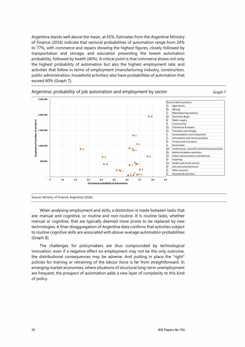
66 BIS Papers No 100
Argentina stands well above the mean, at 65%. Estimates from the Argentine Ministry of Finance (2016) indicate that sectoral probabilities of automation range from 24% to 77%, with commerce and repairs showing the highest figures, closely followed by transportation and storage, and education presenting the lowest automation probability, followed by health (40%). A critical point is that commerce shows not only the highest probability of automation but also the highest employment rate; and activities that follow in terms of employment (manufacturing industry, construction, public administration, household activities) also have probabilities of automation that exceed 60% (Graph 7).
Argentina: probability of job automation and employment by sector Graph 7
Source: Ministry of Finance, Argentina (2016).
When analysing employment and skills, a distinction is made between tasks that
are: manual and cognitive, or routine and non-routine. It is routine tasks, whether manual or cognitive, that are typically deemed more prone to be replaced by new technologies. A finer disaggregation of Argentine data confirms that activities subject to routine cognitive skills are associated with above-average automation probabilities (Graph 8).
The challenges for policymakers are thus compounded by technological innovation: even if a negative effect on employment may not be the only outcome, the distributional consequences may be adverse. And putting in place the “right” policies for training or retraining of the labour force is far from straightforward. In emerging market economies, where situations of structural long-term unemployment are frequent, the prospect of automation adds a new layer of complexity to this kind of policy.
AB
C
D E
F
G
H
I
J K
L
MN
OP
Q
R
S
T
-
500.000
1.000.000
1.500.000
2.000.000
2.500.000
0 0,1 0,2 0,3 0,4 0,5 0,6 0,7 0,8 0,9
Empl
oym
ent (
num
ber o
f wor
kers
)
Estimated probability of automation
Key to labels (sectors)A Agriculture, B MiningC Manufacturing industryD Electricity & gasE Water supplyF ConstructionG Commerce & repairsH Transport and storageI Accomodation and restaurantsJ Information and communicationK Finance and insuranceL Real estateM Professional, scientific and technical activitiesN Administratative activitiesO Public administration and defenceP TeachingQ Health and social serviceR Arts and entertainmentS Other servicesT Household activities
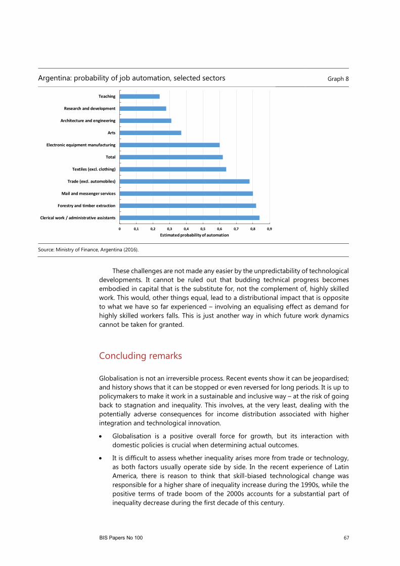
BIS Papers No 100 67
Argentina: probability of job automation, selected sectors Graph 8
Source: Ministry of Finance, Argentina (2016).
These challenges are not made any easier by the unpredictability of technological
developments. It cannot be ruled out that budding technical progress becomes embodied in capital that is the substitute for, not the complement of, highly skilled work. This would, other things equal, lead to a distributional impact that is opposite to what we have so far experienced – involving an equalising effect as demand for highly skilled workers falls. This is just another way in which future work dynamics cannot be taken for granted.
Concluding remarks
Globalisation is not an irreversible process. Recent events show it can be jeopardised; and history shows that it can be stopped or even reversed for long periods. It is up to policymakers to make it work in a sustainable and inclusive way – at the risk of going back to stagnation and inequality. This involves, at the very least, dealing with the potentially adverse consequences for income distribution associated with higher integration and technological innovation.
• Globalisation is a positive overall force for growth, but its interaction with domestic policies is crucial when determining actual outcomes.
• It is difficult to assess whether inequality arises more from trade or technology, as both factors usually operate side by side. In the recent experience of Latin America, there is reason to think that skill-biased technological change was responsible for a higher share of inequality increase during the 1990s, while the positive terms of trade boom of the 2000s accounts for a substantial part of inequality decrease during the first decade of this century.
0 0,1 0,2 0,3 0,4 0,5 0,6 0,7 0,8 0,9
Clerical work / administrative assistants
Forestry and timber extraction
Mail and messenger services
Trade (excl. automobiles)
Textiles (excl. clothing)
Total
Electronic equipment manufacturing
Arts
Architecture and engineering
Research and development
Teaching
Estimated probability of automation
68 BIS Papers No 100
• Technological innovation can have a positive effect on employment, but there is evidence of adverse distributional consequences. The final outcome remains largely open, depending on the policy response. An important part of the answer lies in education and training, but what concrete form these should take remains an open question.
References
Acosta, P and L Gasparini (2007): “Capital accumulation, trade liberalization, and rising wage inequality: the case of Argentina”, Economic Development and Cultural Change, vol 55, pp 793–812.
Autor, D (2015): “Why are there still so many jobs? The history and future of workplace automation”, Journal of Economic Perspectives, vol 29, no 3, pp 3–30.
Bolaky, B and C Freund (2004): “Trade, regulations and growth”, World Bank Policy Research Working Papers, no 3255, Washington DC.
De la Torre, A, A Ize, G Beylis and D Lederman (2015): “Jobs, wages and the Latin American slowdown”, LAC Semiannual Report, World Bank, Washington DC, October.
Estevadeordal, A and A Taylor (2013): “Is the Washington consensus dead? Growth, openness, and the Great Liberalization, 1970s–2000s”, Review of Economics and Statistics, vol 95, no 5, pp 1669–90, December.
Galiani, S and P Sanguinetti (2003): “The impact of trade liberalization on wage inequality: evidence from Argentina”, Journal of Development Economics, vol 72, no 2, pp 497–513, December.
Gasparini, L, G Cruces and L Tornarolli (2016): “Chronicle of a deceleration foretold: Income inequality in Latin America in the 2010s”, CEDLAS Working Papers, no 198, Universidad Nacional de La Plata, May.
Gerchunoff, P and L Llach (2009): “Equality and growth: a 20th century Argentine dilemma”, Journal of Iberian and Latin American Economic History, vol 27, no 3, pp 397–426.
Giordano, P and K Li (2012): “An updated assessment of the trade and poverty nexus in Latin America”, Inter-American Development Bank Working Paper Series, no IDB-WP-383, November.
Goldin, C and L F Katz (2008): The Race Between Education and Technology, Cambridge, MA: Harvard Univ. Press.
Hopenhayn, H and A Neumeyer (2005): “Explaining Argentina’s Great Depression of 1975–90”, in E Fernandez-Arias, R Manuelli and J Blyde (eds) Sources of Growth in Latin America. What is Missing, Inter-American Development Bank.
Kremer, M (1993): “The O-ring theory of economic development”, Quarterly Journal of Economics, vol 108, no 3, pp 551–75.
Lachmann, L (1977): Capital, expectations, and the market process: essays on the theory of the market economy, Kansas City: Sheed Andrews and McMeel.

BIS Papers No 100 69
Ministry of Finance, Argentina (2016): “Estimaciones preliminares sobre la automatización del empleo en Argentina”, Estudios sobre Planificación Regional y Sectorial, year 1, no 1, December.
Rodríguez, F and D Rodrik (2001): “Trade policy and economic growth: a skeptics guide to the cross-national evidence”, NBER Macroeconomics Annual 2000, vol 15, pp 261–38.
Sachs, J and A Warner (1995): “Economic reform and the process of global integration”, Brookings Papers on Economic Activity, vol 26, no 1, pp 1–118.
World Bank (2016): World Development Report 2016: Digital Dividends, Washington, DC: World Bank.

70 BIS Papers No 100

BIS Papers No 100 71
Globalisation and deglobalisation
Central Bank of Brazil
Abstract
In the years before the global financial crisis, emerging market economies (EMEs) saw robust global demand, substantial improvements in terms of trade and abundant capital inflows. Nevertheless, trade growth has been weak after the financial crisis, and whether this movement is permanent or transient is still an open question. This note discusses trends in globalisation, the macroeconomic and distributional effects of globalisation in EMEs, and complementary policies that may enable countries to better seize the benefits of globalisation, highlighting the Brazilian experience.
Keywords: globalisation, emerging market economies, complementary policies.
JEL classification: F15, F60.

72 BIS Papers No 100
Determinants of globalisation in EMEs: trade, GVCs and financial integration
The growth of international trade in emerging market economies (EMEs) over the last two decades was driven mainly by favourable external conditions. Before the Great Financial Crisis (GFC), EMEs saw robust global demand, substantial improvements in terms of trade and abundant capital inflows from advanced economies (AEs), which helped to finance trade and production. Higher global demand for commodities, especially from 2000 to 2011, boosted prices and trade volumes, increasing the share of EMEs in international trade. More recently, the long-lasting AE policy responses to the GFC have also benefited EMEs. Abundant liquidity has financed consumption, exports and investments in these economies, leading to more globalisation.
Nevertheless, trade growth has been weak post-crisis, and whether this shift is permanent or transitory is still an open question. Before the GFC, global trade frequently grew faster than GDP. After the crisis, trade recovered during 2010–11, but slowed again from 2012 onwards. The annual growth rate of global trade during the 2012–15 period (roughly 3%) was smaller than the pre-crisis average (7% for the 1987–2007 period) and slightly smaller than the world GDP growth rate, in real terms.1
Recent studies have highlighted the composition of global GDP growth to explain the slow pace of trade growth after the GFC.2 During the past 20 years, the share of EMEs in global growth roughly doubled, as well as their participation in trade, which increased from 20% to almost 40%. As EMEs have lower trade-income elasticities compared to AEs, the upsurge of EMEs in international trade and GDP lowered global trade-income elasticity. However, elasticity is not a constant parameter. In the long run, EME growth can lead to higher trade-income elasticity, strengthening trade growth.
The declining growth of global value chains (GVCs) may also be driving the slowdown in trade growth. Despite the rapid expansion from 1995 to 2011, the growth of GVCs has stalled in recent years.3 Although this result is partially due to cyclical factors, notably a slowdown in central economies, there are structural reasons that may lead to a long-lasting stagnation in GVCs, such as the rise in labour costs in EMEs, the tightening of global financial conditions and the development of intermediate input sectors in China. Concerning the latter, a recent study points out that China’s domestic content in exports increased from 65% to 70% in the 2000–07 period, due to the substitution of domestic for imported materials by exporters. These results indicate that China is relying less on foreign materials and becoming more competitive in intermediate input sectors.4 In addition, greater complexity and large capital demands make GVCs more vulnerable to global financial conditions.
Looking forward, the response to possible protectionist measures in some AEs is also a source of concern. In a scenario of increased protectionism, a new suboptimal equilibrium might emerge, in which affected countries could react,
1 Constantinescu et al (2015).
2 ECB-IRC Trade Task Force (2016) and Deutsche Bundesbank (2016).
3 ECB-IRC Trade Task Force (2016).
4 Kee and Tang (2016).

BIS Papers No 100 73
leading to further protectionist measures and potentially damaging global trade. In response to more protectionism, firms could postpone or even cancel long-term investments, or lose their inclusion in trade chains, which would take time to be rebuilt in the future.
Technological innovations, on the other hand, may influence GVCs and spur the growth of global trade in the years ahead. The digital revolution has promoted the access of small and medium-sized enterprises (SMEs) to foreign markets and expanded global services trade. Digital platforms have changed market structures and promoted higher competitiveness in cross-border trade, as it has reduced the cost of international interactions and transactions that used to preclude SMEs from supplying goods and services abroad. Not only are more firms engaged in international trade currently, but also the nature of trade has changed over time, including the expansion of global trade of digitally deliverable services, such as financial services, IT support, customer services, engineering and design. However, services trade is still a small fraction of global trade.5 In Brazil, 48 million consumers made at least one virtual purchase in 2016, representing an increase of 22% over 2015. The amount that Brazilian e-consumers spent in cross-border purchases also increased 17% in the same period, and is expected to continue to grow in the coming years.6
In addition to trade integration, globalisation has also led EMEs to higher financial integration. Besides the direct benefit of providing more access to financing capital from abroad, financial integration also promotes the improvement of institutions, the enhancement of market discipline and the depth of the financial sector. However, these indirect benefits are not easily measured and are only accomplished in the medium term. Overall, the literature supports the view that EMEs have on the whole benefited from financial integration, although this has also increased their exposure to financial crises. In this sense, there are preconditions that lead EMEs to obtain better outcomes from financial liberalisation, such as robust macroeconomic policy framework, financial sector development, and openness to trade.7 In any case, domestic and international macroprudential policies are important in building a sound and resilient financial sector to counteract possible exposure effects.
Besides, there is evidence that trade openness decreases countries’ vulnerability to financial crisis8. Trade integration has helped EMEs to manage financial crises associated with sudden stops of capital inflows, through balance sheet effects. After cut-offs in external financing, economies that are less open to trade generally need larger real exchange rate depreciations to improve their trade balance. As a result, they may experience an increase in firms’ liabilities denominated in foreign currency, an increase in default probabilities, and a reduction in the country’s output growth rates. Trade balance adjustments in more open economies do not require larger depreciations and, thus, are likely to be less costly. Studies also claim that trade openness decreases the probability of reversals in capital inflows, as exchange rate
5 McKinsey Global Institute (2016).
6 Webshoppers (2017).
7 Kose et al (2006) and Obstfeld (2009)
8 Calvo et al (2004), Frankel and Cavallo (2004) and Cavallo (2005).
74 BIS Papers No 100
depreciations may boost export revenues and increase the country’s ability to service its external debt.9
Globalisation: macroeconomic effects
There is an open debate regarding the benefits and costs of globalisation for developing countries, but the most accepted view is that, over the last two decades, globalisation has indeed been a positive driving force for growth in EMEs. The results are, however, very dependent on the group of countries considered and the domestic policies in place. EME growth now represents close to 80% of total global growth, and EMEs’ increased participation is linked to the expansion of international trade.10 In the case of Latin America, the evidence indicates that the impact of trade openness on growth was positive but mostly small.11 It also suggests that episodes of trade liberalisation were significantly correlated with macro and micro reforms.12
In 1988–90, Brazil experienced a singular episode of trade openness through tariff reductions that withdrew market protection quite abruptly from several manufacturing industries. Evidence shows that there were positive effects on productivity growth after the elimination of trade barriers. On average, total factor productivity grew at a 3% yearly rate, while labour productivity grew above 5%.13 Higher productivity growth after trade liberalisation resulted from two mechanisms: more competition in domestic markets and access to foreign inputs that embodied better technology.14
However, a more competitive environment does not necessarily lead to higher output in all sectors. In the case of Brazil, there was a change in the economy’s sectoral composition. The production share of the manufacturing sector fell, while the impact was positive on services. Some factors were important in this context: (i) low growth in advanced countries depressed the international prices of manufacturing products; and (ii) currency appreciation reduced the relative competitiveness of the Brazilian manufacturing sector. The third and fourth factors concern the domestic policy response to the GFC: (iii) reduced interest rates; and (iv) more flexible fiscal policy and credit to stimulate domestic demand. Expanded demand for services increased real wages, while the combination of higher real wages and stagnating labour productivity in the manufacturing sector led to a fall in production.15
9 Kose et al (2006) and IMF (2002).
10 IMF (2017).
11 Giordano and Li (2012).
12 Rodriguez and Rodrik (2001).
13 Ferreira and Rossi (2003).
14 Lisboa et al (2010) and Schor (2004).
15 Pastore et al (2012).

BIS Papers No 100 75
Increased international trade and financial integration have also resulted in more synchronised business cycles, as shocks are transmitted between countries through their trade flows. Earlier evidence supported the view that there was convergence of business cycles among industrial countries and among EMEs, but divergence between the two groups.16 More recently, evidence has emerged suggesting a rise in global business cycle synchronisation from 2000 onwards.17, 18 In the case of Brazil, the business cycle seems to be synchronised with the global economy, but less so at the regional level.19
In Brazil, the results from an estimated DSGE model indicate that trade globalisation has reduced inflation via imported goods. The mechanism goes as follow: since imported and local produced goods are complementary to each other on average, trade globalisation reduces artificial import costs and then jointly improves imports, local production and terms of trade, while reducing marginal production costs. The improvement in terms of trade again increases goods imports, lifting the local goods supply and putting additional downward pressure on domestic inflation. Conversely, imposing trade barriers – for instance increasing import taxes – positively affects the inflation rate.20
It also seems that financial openness has contributed to external stability, by enhancing resilience. In Brazil, improvements in the balance of payments since 2005 have allowed the Central Bank of Brazil (BCB) to accumulate a sizeable amount of foreign reserves, currently in excess of USD 380 billion, around 20% of Brazilian GDP. Likewise, foreign direct investment (FDI) continues to be the main source of external financing to Brazil.21 In addition to increasing the capital stock and the level of technology, FDI tends to be more stable and less correlated to debt or portfolio flows, and hence less prone to sudden reversals.22
Globalisation: distributional effects
Another key issue is the impact of trade integration on wage inequality. There is evidence that, when trade opening induces technological change, it tends to introduce comparative gains for higher skilled workers in both skill-abundant and skill-scarce countries.23 Evidence also indicates that trade opening contributes to a skill-biased technological change in a wide sample of countries,
16 Kose et al (2008).
17 Ductor and Leiva-Leon (2017).
18 Such an increase in business cycle synchronisation is mainly attributed to EMEs, and more specifically to a group comprising Argentina Brazil, Bulgaria, Chile, China Malaysia, Mexico, the Philippines, Romania, South Africa and Venezuela. Data also indicate that business cycle co-movements are explained by financial openness, government expenditure, bilateral trade, human capital, liquid liabilities and similarities between countries’ industrial composition.
19 Gutierrez and Gomes (2009) and Correa (2003).
20 Santos and León (2010).
21 Goldfajn and Minella (2005) and Central Bank of Brazil (2017).
22 Goldfajn and Minella (2005).
23 Acemoglu (2003).

76 BIS Papers No 100
including those of Latin America.24 Considering that protectionist policies shield export sectors that heavily employ unskilled labour in EMEs, it is not surprising that, initially, trade opening negatively affects these workers’ wages. Nevertheless, evidence shows that, in some cases, trade liberalisation has not caused wage inequality.
In Brazil, trade reforms did not induce an increase in wage inequality between skilled and unskilled workers. No effect on informality was found either.25 In fact, there is evidence that trade liberalisation reduced earnings discrepancies in Brazil.26 The mechanism is that pre-liberalisation tariffs adjusted by import penetration were higher in skill-intensive sectors and fell more than in other protected industries. This led to a decline in their relative prices after the tariff reduction process and, consistent with Stolper-Samuelson theorem, this decline produced a decrease in skilled wages and an outflow of workers from these protected sectors.
However, the evidence suggests that displaced workers from more protected industries were not absorbed by exporting firms or those industries with comparative advantages.27 After Brazilian trade liberalisation, evidence based on micro-data indicates that production shifted to more productive firms, but displaced labour did not follow. As a side effect of the trade reform, Brazilian economy observed higher rates of failed labour reallocations and longer durations of complete reallocations.
On the other hand, simulations of additional trade liberalisation reforms in Brazil show that the expansion in investment and production could provide significant employment gains. Moreover, the sectoral analysis of these results indicates that employment growth would be higher for low-skilled workers, helping those at the lower end of the income distribution.28
Regarding the effects of openness on poverty, the literature has not reached a consensus. It is not clear which indicators would be more appropriate to measure openness nor what its causal relationship to poverty standards is. Export measures are associated with decreasing poverty, while reductions of import content are related to rising poverty.29 Studies for Latin America are not conclusive as to the role of openness in explaining changes in poverty and income inequality.30 The findings usually depend on domestic policies and institutions.31 Similar inconclusive results arise for Brazil in a study that focuses on trade liberalisation.32
24 Berman et al (1998), Berman and Machin (2000) and Sanchez-Páramo and Schady (2003).
25 Goldberg and Pavcnik (2003).
26 Gonzaga et al (2006) and Ferreira et al (2007).
27 Menezes-Filho and Muendler (2011).
28 Araújo and Flaig (2016).
29 Harrison (2005).
30 Bouzas and French-Davis (2003).
31 Behrman et al (2003).
32 Ventura-Dias (2005).

BIS Papers No 100 77
Policy implications and final remarks
Adequate complementary policies help to promote the positive impact of trade opening on growth, particularly for higher investment in human capital, deeper financial markets, lower inflation, and greater availability of public infrastructure. These features provide the necessary conditions for improving the competitiveness of domestic firms by supporting the development of a better-educated labour force, a stable macroeconomic environment with less expensive credit, and better-quality infrastructure.33
Structural reforms have the potential to harness the benefits of globalisation and boost growth. Removing trade barriers helps to reduce the cost of imported inputs and to strengthen incentives to enhance productivity. Besides, stronger trade integration benefits low-income earners in particular, as an expansion of the export sector has a larger impact on the demand for low-skilled labour. Improvements in infrastructure could also reduce transportation costs, particularly for exporters. Further improvements in educational attainment would not only raise productivity, but also allow more low-income households to join Brazil’s growing middle class.34
In this regard, Brazil has improved its policy framework and implemented new structural domestic policies aiming at improving macro and micro fundamentals. Among these recent reforms and adjustments, it is worth mentioning labour reform, educational reform, the constitutional spending ceiling, reforms in the oil and gas sector, privatisations, and the reform of the Brazilian Development Bank’s interest rates.35
Countries can best take advantage of globalisation and mitigate its harmful effects by adopting an appropriate complementary policy mix. As globalisation generates losers and winners, especially across sectors, policies should support natural winners and facilitate labour transition among different sectors. At the same time, appropriate safety nets can be put in place to protect the most vulnerable workers and potential losers.36 Active labour market programmes should be set up to help unemployed workers find new jobs. Training, counselling, placement services, and assistance in job searches are among the most common examples.37 In this regard, Brazil has recently approved a labour reform to increase the flexibility and efficiency of its labour market.
The more dynamic environment brought by globalisation calls for new types of social protection. To get reforms under way may require one-time compensation schemes for workers who would otherwise lose out, such as well designed unemployment insurance and severance pay systems. Social protection is important not just to support families that may stand to lose in the more dynamic economy, but also to create a solid social foundation from which people feel
33 Chang et al (2009).
34 OECD (2017).
35 Goldfajn (2017).
36 Harrison (2005).
37 World Bank (2002).

78 BIS Papers No 100
comfortable taking risks and pursuing entrepreneurship.38 Globalisation also calls for social protection for immigrants. In this respect, the Brazilian government published in 2017 a new immigration law that promulgates new rights for immigrants, such as free access to social and public health programmes. The law also guarantees broad access to judicial institutions and free legal support for poor immigrants.39 Having said that, immigration flows into Brazil are still small. By December 2015, there were 0.7 million non-native people living in Brazil, or 0.3% of the country’s population.40
In recent decades, Brazil has also successfully put in place a set of policies to support the most vulnerable population. The literature suggests that the increasing level of human capital accumulation and the expansion of conditional cash transfer programmes has led to a great fall in inequality. Brazil should therefore continue to expand its investment in education and to improve its cash transfer mechanisms with the aim of helping recipients find a way out of poverty by participating in the labour market. Finally, it is important to promote institutional reforms to speed up the process of creating new firms, to reduce the tax burden levied on small firms, and to make the cost of hiring formal employees less expensive.41
The degree of openness to the global economy has not changed much in Brazil over the last two decades.42 Although trade flows have greatly increased over this period, this has had more to do with the commodities supercycle than with trade openness. In fact, the favourable economic environment in the 2000s led to more protectionism in Brazil. In recent years, however, the incentives have changed, and the government has started to remove some protectionist measures. The recent decision to ease local content rules is one step towards reducing trade barriers.43 The literature using computable general equilibrium (CGE) models suggests that there is room for trade expansion with a positive impact on growth. Reductions in import tariffs and local content requirements, along with other structural reforms, could lead to stronger industrial development and higher export competitiveness.
Despite the widespread impact of globalisation, the implications for monetary policy seem to be much more contained. The general objective of monetary policy – price stability – remains unchanged, as do the main strategies for achieving it, such as inflation targeting. Most importantly, central banks have retained their ability to meet their targets in both AEs and EMEs.
Macroprudential measures have played an important role in guaranteeing financial stability as well as in addressing external shocks. One of the distinguishing features of the Brazilian economy is its prudential regulatory framework. The vigilant stance of the central bank has prevented the development of disequilibria and excesses in Brazil.44
38 World Bank (2002).
39 KPMG (2017).
40 United Nations (2015).
41 Menezes-Filho and Scorzafave (2012).
42 Neves (2014).
43 OECD (2017).
44 Meirelles (2009).

BIS Papers No 100 79
The Central Bank of Brazil has also contributed to important reforms of the financial system through its BC+ public agenda.45 Structured in four pillars, the Agenda BC+ aims at (i) increasing financial citizenship; (ii) improving the central bank’s legal framework; (iii) increasing the efficiency of the financial system; and (iv) reducing credit costs. Examples of actions of the Agenda BC+ include contributions for the regulation of electronic registration of collateral and guarantees; the law setting a market-oriented interest rate (TLP) for the Brazilian Development Bank; and the establishment of a new credit bureau.
In summary, it seems that globalisation forces are weakening, given slow trade growth, tighter immigration policies and the increased risk of protectionist measures in AEs. However, it is too early to conclude that these changes represent a trend to deglobalisation rather than a cyclical decline. In any case, EMEs should take advantage of international liquidity and low financing costs to fuel globalisation. Policy reforms, such as reductions in import tariffs, along with other structural reforms would increase EMEs’ inclusion in global trade, positively affecting exports, investment and production. This is the right way to take advantage of globalisation and mitigate its negative impacts. The global outlook is challenging, but there are also prospective opportunities for EMEs. Rather than fomenting a backlash, EMEs should reinforce the engine of globalisation, especially by filling trade gaps and strengthening trading relationships.
45 Central Bank of Brazil (2016).

80 BIS Papers No 100
References:
Acemoglu, D (2003): “Patterns of Skill Premia”, Review of Economic Studies, vol 70.
Araújo, S and D Flaig (2016): “Quantifying the effects of trade liberalisation in Brazil: a CGE model simulation”, OECD Working Papers, no 1295.
Behrman, J, N Birdsall and M Szekely (2003): “Economic Policy and Wage Differentials in Latin America”, Center of Global Development Working Paper, no 29.
Berman, E, J Bound and S Machin (1998): “Implications of skill-biased technological change: international evidence”, Quarterly Journal of Economics, vol 113.
Berman, E and S Machin (2000): “Skill-biased technology transfer around the world”, Oxford Review of Economic Policy, vol 16, no 3, September.
Bouzas, R and R French-Davis (2003): “Globalization and equity: a Latin American perspective”, paper presented at the Fourth Annual Conference on Global Development, Cairo.
Calderon, C, A Chong and E Stein (2007): “Trade intensity and business cycle synchronization: are developing countries any different?”, Journal of International Economics, vol 71.
Calvo, G, A Izquierdo and L Mejia (2004): “On the empirics of sudden stops: the relevance of balance-sheet effects”, NBER Working Papers, no 10520.
Cavallo, E (2005): “Output volatility and openness to trade: a reassessment”, manuscript, Kennedy School of Government, Harvard University.
Central Bank of Brazil (2017): “Inflation Report”, vol 19, no 3, September.
——— (2016): “Agenda BC+”, December, www.bcb.gov.br/pec/appron/apres/Apresenta%C3%A7%C3%A3o_Presidente_Ilan_Goldfajn_Agenda_BC_Mais_20122016.pdf.
Constantinescu, C, A Matoo and M Ruta (2015): “The global trade slowdown: cyclical or structural?”, IMF Working Papers, no 2015/6.
——— (2016): “Does the global trade slowdown matter?”, Policy Research Working Papers, no 7673, World Bank Group.
Correa, A (2003): “Diferenças e Semelhanças entre Países da América Latina: Uma Análise de Markov Switching para os Ciclos Econômicos de Brasil e Argentina”, Central Bank of Brazil, Trabalhos para Discussão.
Chang, R, L Kaltani and N Loayza (2009): “Openness can be good for growth: the role of policy complementarities”, Journal of Development Economics, vol 90.
Deutsche Bundesbank (2016): Monthly Report, March.
Ductor, L and D Leiva-Leon (2016): “Dynamics of global business cycle interdependence”, Journal of International Economics, no 102.
Ferreira, P and J Rossi (2003): “New evidence from Brazil on trade liberalization and productivity growth”, International Economic Review, vol 44.
Ferreira, F, P Leite and M Wai-Poi (2007): “Trade liberalization, employment flows and wage inequality in Brazil”, World Bank Policy Research Working Papers, no 4108.

BIS Papers No 100 81
Frankel, J and E Cavallo (2004): “Does openness to trade make countries more vulnerable to sudden stops or less? Using gravity to establish causality”, NBER Working Papers, no 10957.
Frankel, J and A Rose (1998): “The endogeneity of the optimum currency area criteria”, Economic Journal, vol 108.
Giordano, P and K Li (2012): “An update assessment of the trade and poverty nexus in Latin America”, IDB Working Paper Series, no 4209.
Goldberg, P and N Pavcnik (2004): “Trade inequality and poverty: what do we know? evidence from recent trade liberalization episodes in developing countries”, NBER Working Papers, no 1059.
——— (2003): “The response of the informal sector to trade liberalization”, Journal of Development Economics, vol 72, pp 463–96.
Goldfajn, I (2017): “Brazil – the road ahead”, Financial Times Conference, New York, September.
Goldfajn, I and A Minella (2005): “Capital flows and controls in Brazil: what we have learned?”, NBER Working Papers, no 11640, September.
Gonzaga, G, N Menezes Filho and M Terra (2006): “Trade liberalization and the evolution of skill earnings differentials in Brazil”, Journal of International Economics, vol 68, no 2, pp 345–67.
Gutierrez, C and F Gomes (2009): “Evidence on common feature and business cycle synchronization in Mercosur”, Brazilian Review of Econometrics, vol 29, no 1, pp 37–58, May.
Harrison, A (2005): “Globalization and poverty”, NBER Working Papers, no 12347.
Imbs, J (2004): “Trade, finance, specialization, and synchronization”, Review of Economics and Statistics, vol 86.
International Monetary Fund (2002): World Economic Outlook, September.
——— (2017): World Economic Outlook, April.
European Central Bank (2016): International Relations Committee (IRC) Task Force, “Understanding the weakness in global trade: what is the new normal?”, ECB Occasional Paper, no 178, September.
Kee, H and H Tang (2016): “Domestic value added in exports: theory and firm evidence from China”, American Economic Review, vol 106.
Kose, M, E Prasad, K Rogoff and S Wei (2006): ”Financial globalization: a reappraisal”, NBER Working Papers, no 12484.
Kose, M, C Otrok and E Prasad (2008): “Global business cycle: convergence or decoupling”, NBER Working Papers, no 14292.
KPMG, GMS Flash Alert, Immigration Edition, June 2017.
Lisboa, M, N Menezes-Filho and A Schor (2010): “The effects of trade liberalization on productivity growth in Brazil: competition or technology?”, Revista Brasileira de Economia, vol 64, no 03.
McKinsey Global Institute” (2016): Digital globalization: the new era of global flows, March.

82 BIS Papers No 100
——— (2016):”People on the move: global migration’s impact and opportunity”, December.
Meltzer, J (2016): “Maximizing the opportunities of the internet for international trade”, The E15 Initiative Policy Options Paper, January.
Menezes-Filho, N and M Muendler (2011): “Labour reallocation in response to trade reform”, NBER Working Papers, no 17372.
Menezes Filho, N and L Scorzafave (2012): “Employment and inequality of outcomes in Brazil”, Insper Policy Papers, no 1.
Meirelles, H (2009): “Ten years of floating exchange rates in Brazil”, speech by the Governor of the Central Bank of Brazil.
Neves, J (2014): “Brazil´s slow and uncertain shift from trade protectionism to free trade”, Inter-American Dialogue Working Paper.
Obstfeld, M (2009): "International finance and growth in developing countries: what we have learned?”, NBER Working Papers, no 14691.
OECD (2017): Economic Outlook, no 1.
Pastore, A, M Gazzano and M Pinotti (2012): “Por que a produção industrial não cresce desde 2010?”, A.C. Pastore e Associados, manuscript.
Ratha, D, S Mohapatra and E Scheja (2011): “Impact of migration on economic and social development”, Policy Research Working Paper, no 5558, World Bank Group.
Rodríguez, F and D Rodrik (2001): “Trade policy and economic growth: a skeptics guide to the cross-national evidence”, NBER Macroeconomics Annual.
Sánchez-Páramo, C and N Schady (2003): “Off and running? Technology, trade, and the rising demand for skilled workers in Latin America”, World Bank Policy Research. Working Paper, no 3015, Washington DC.
Santos, R and M León (2010): “Efeitos da Globalização na Inflação Brasileira”, Central Bank of Brazil, Trabalhos para Discussão, no 201.
Schor, A (2004): “Heterogeneous productivity response to tariff reduction. Evidence from Brazilian manufacturing firms”, Journal of Development Economics, vol 75, December.
United Nations (2015): Department of Economic and Social Affairs – Population Division, International migrant stock as a percentage of the population, www.un.org/en/development/desa/population/migration/data/estimates2/estimates15.shtml.
Ventura-Dias V (2005): “Os Aspectos Distributivos das Negociações Comerciais: o Estado do Debate no Brasil”, Latin America Trade Network Working Papers, no 33.
Webshoppers (2017): Relatório, no 35, February.
World Bank (2002): Globalization, growth, and poverty, World Bank and Oxford University Press.

BIS Papers No 100 83
Globalisation and the Chilean economy
Joaquin Vial1
Abstract
This note describes and analyses Chile’s economic integration into the global trading system, including the impact on goods, services, capital and labour. This was a gradual process starting in the mid-1970s. Currently Chile is a very open economy, even though immigration is a relatively new phenomenon which is already having an impact at the macroeconomic level. During this period, there have been significant institutional developments, notably the establishment of the central bank’s independence, with a clear mandate to control inflation and a ban on funding of the government. New fiscal rules are designed to isolate the public finances from short-term cyclical fluctuations and volatile copper prices. The adoption of inflation targeting with a free flotation policy in the early 2000s has become a cornerstone of the macroeconomic policy framework. Financial integration has helped to significantly reduce the cost of capital in the country, while providing pension funds with a valuable way of diversifying risks. Chile exhibits some of the largest measures of financial markets depth among emerging market economies (EMEs). Finally, inward FDI has made a large contribution to the development of the country’s productive capacity. In recent years, outward FDI, especially within the region, has helped major Chilean corporations, mostly in the service sector, to expand beyond the limits imposed by the small size of the domestic market.
Keywords: Trade liberalisation, financial opening, floating exchange rate, inflation targeting, immigration
JEL classification: E58, F22, F41, F62.
1 Member of the Board, Central Bank of Chile. Andrea Mostajo provided very able and enthusiastic
help.

84 BIS Papers No 100
Introduction
This note describes and analyses the process of Chile’s economic integration into the global trading system, including the impact on goods, services, capital and labour. This process started in the mid-1970s, after the country abandoned the so-called import substitution model of development. The impact on Chile of similar processes in other EMEs is also discussed, especially the emergence of China as a major industrial centre, with a focus on the main macroeconomic variables of interest for the central bank.
The note is organised as follows: Section 1 presents a summary review of Chile’s integration into the global economy. Since this was a gradual process, several phases are distinguished. Section 2 assesses the effects of globalisation on the main macroeconomic variables and policies, with a particular focus on inflation and monetary policy. Section 3 presents evidence on the characteristics and impact of migration. Section 4 is devoted to the analysis of the potential economic effects of a move towards more protectionism in the advanced economies. The last section concludes.
Chile’s integration into the global economy
After the 1930s Depression, Chile embraced an import substitution strategy for development, erecting a large and cumbersome set of trade restrictions, including both tariff and non-tariff barriers and restrictions on access to foreign exchange. The banking system was subject to quantitative controls and interest rates were regulated. That crisis and the ensuing default meant that Chile remained excluded from external financial markets for more than 40 years, while various nationalisations discouraged FDI. By the end of the 1960s, the economy was suffering periodic foreign exchange crises, followed by devaluations and high inflation, fuelled in part by fiscal deficits financed by monetary expansion. High and volatile inflation became a distinctive feature of the Chilean economy and, by the mid-1960s, economic growth had slowed significantly. In terms of per capita GDP, the country was losing ground against not only the advanced economies, but also within the region. Rapid population growth put pressure on the social and political system. Even though there were major advances in the coverage of education, health services and housing, social and political tensions culminated in a breakdown of democratic institutions in the mid-1970s.2 A massive programme of economic liberalisation and markets reforms was enacted under military rule after the coup in 1973, starting Chile’s re-integration into the global economy.3
a. Phase 1. 1975–90: the initial opening of the economy amid general economic liberalisation and macroeconomic stabilisation
2 For further details on the Chilean experience with import substitution, see Ffrench–Davis (1973),
Collier and Slater (1996) and Meller (1998). At the time, most countries in the region followed similar policies. See for instance, Thorp (1998) and Dornbusch and Edwards (1991).
3 See for instance Larraín and Vergara (2000) and Ffrench-Davis (2010). For a more specific focus on trade liberalisation and exports, Meller (1996). On reforms and macroeconomic performance, Schmidt-Hebbel (2006).

BIS Papers No 100 85
The collapse of the political system in 1973 took place in the midst of a major economic crisis, reflected in widespread shortages of all kind of goods, and inflation running above 500%. The opening of the economy took place at the same time as other reforms and a severe stabilisation programme were implemented. In this period most non-tariff barriers were abolished, tariffs were brought down and unified at 10% in 1977, and most exchange controls were eliminated. FDI restrictions were lifted after a new law was enacted in 1974.4 The central bank set the value of the exchange rate, with periodic adjustments to keep up with inflation. In 1979 it was set at a fixed nominal value (inflation was still running above 30% at the time), while at the same time the capital account was liberalised.
The combination of financial liberalisation with a fixed exchange rate ended badly in 1982, after a worsening in international conditions made it impossible to finance huge current account deficits. The economy fell into the deepest recession since the 1930s, and the financial system collapsed after large devaluations that year.
There was a partial reversal of trade liberalisation after tariffs were increased to 35%, but then they were gradually brought down to 15% at the end of the decade. FDI flows began to pick up in this period. In addition to some large copper mining projects, foreign capital also went to recently privatised state companies, such as telecoms. An aggressive programme of debt-equity swaps also attracted foreign (and domestic) investors to all sectors of the economy.
By the end of the decade the economy had experienced a major transformation as shown in the charts in Annex A, with a larger participation of foreign trade in GDP, a significant diversification of exports and imports, in terms of both their composition and international partners. However exports remained biased towards natural resources-based goods and there was very little integration into global value chains. The end of protectionism meant that consumers and firms had access to wide range of products and services previously prohibited or too expensive. As expected, imports displaced domestic manufactures, especially in durable goods, with a significant impact on employment. Traditional agriculture, oriented towards the production of highly protected food (grains, meat) had to readjust, but in most cases this sector benefited from new opportunities for exports of higher value products such as fruit. The expansion of forest plantations to support future exports also created value in non-arable areas. Strong export demand for products such as fish and seafood, as well as wood pulp, put significant pressure on the environment, leading in some cases to over-extraction and even the collapse of some fisheries.5
b. Phase 2: 1990–mid-2000s: Free trade agreements, the emergence of EMEs as export markets, financial integration, and the first steps in the internationalisation of Chilean companies
This period marks the consolidation of the economic opening. After the return to democracy, governments maintained and deepened the integration into the world economy. General tariffs were brought down to 11% in 1991, and then to 6% in 1998,
4 This led Chile to withdraw from the Andean pact, a subregional trade pact requiring substantially
more restrictive rules for FDI.
5 See for instance World Bank (1994) and Figueroa et al (1996). In the 1990s environmental issues played an increasingly important role in the political and economic agenda, as pollution and other environmental problems associated with sustained economic growth became more evident. Globalisation also played a role here, as international conventions and market reactions provided an impulse to set higher environmental standards.

86 BIS Papers No 100
in response, respectively, to the oil price shock caused by the first Gulf War and to the Asian Crisis. In this period, Chilean governments pursued an active policy of signing free trade agreements, so that by the end of this decade Chile had signed or was negotiating FTAs with all major trade partners.
This period coincided with the emergence of the Asian “tiger” EMEs and then China. This process had a deep effect on Chile. On the exports side, the Asian EMEs became large importers of metals and other industrial raw materials (minerals, timber), and later of consumer goods, such as food and wine. These countries began to gain importance at the expense of other traditional markets such as the United States and Europe. On the other hand, these EMEs also gained a large market share in Chilean imports of low-priced manufactured consumer goods (clothing, electrical appliances, vehicles and computers).
In the late 1980s and early 1990s, some institutional changes took place. The new central bank law established the institution’s independence, providing for a monetary policy with the sole objective of controlling inflation. Meanwhile, the Copper Stabilisation Fund was set up with the aim of dampening the traditional cyclical influence of copper prices on fiscal expenditure. The combination of both elements allowed for further reductions in inflation, which came down to international levels by the end of the decade, while turning the public sector into a net creditor
Inflows of FDI were large during this era, especially in mining, other natural resources and services, including energy and financial services. Later, a few large Chilean companies began expanding abroad, especially in services (electricity, retail).
During the second half of this period, Chile’s pension funds were allowed to invest a larger fraction of their assets abroad. The outflow began very slowly, due to large interest rate differentials, but as the economy made progress, domestic interest rates fell and institutional investors began to invest abroad more aggressively, especially after the Asian crisis.
c. Phase 3: 2005–present: consolidation of international integration, active
expansion of Chilean companies abroad and growing immigration
This later phase is characterised by the consolidation of trade and financial integration, a process that continued in spite of the Great Financial Crisis (GFC) in 2007–09. During this period, China became Chile’s main trade partner, both in exports and imports. Also, most major Chilean companies reached the limits of their expansion in the domestic market, and began looking for opportunities abroad, taking advantage of economic reforms in the region.6 Major Chilean investments in the rest of region are in transportation (airlines), retail, pulp and paper and, to a lesser extent, financial services.
Finally, immigration from neighbouring countries started to gain momentum in the 1990s, especially from Peru at the outset, followed by Argentina after the crisis in the early 2000s, and more recently from Colombia, Venezuela and the Caribbean (Haiti, in particular). Some of these immigrants have high levels of education and have joined Chilean companies in professional-level roles, but most are low-skilled workers
6 At the same time, companies from other countries in the region, particularly Colombia, Peru and
Brazil, began to invest in Chile.
BIS Papers No 100 87
who have helped sectors such as agriculture, construction and services to regain their competitiveness.
Globalisation and its impact on macroeconomic policies
This section, first, reviews the effect of globalisation on the inflation rate, as a result of changes in relative prices of some consumption goods, especially durables. Second, it assesses how policies and institutions dealt with macroeconomic volatility linked to external shocks and, third, it discusses the evidence for changes in the level and volatility of the exchange rate before and after the adoption of inflation targeting and the free flotation of the currency.
a. Direct impact of globalisation on inflation
The elimination of trade barriers is likely to affect short-term inflation – more so in a highly indexed economy as the Chilean one – due to the fall of prices in importable goods. This change could be large in the case of heavily protected industries – such as automobiles, for instance – and as new opportunities for consumption arise, they might become more important as these same goods increase their share in the CPI.
In Chile, this first-order effect was felt in the late 1970s, a period of rampant inflation with severe measurement distortions, so that it would be very difficult to measure the impact accurately. Then, as inflation fell and new low-cost producers such as China emerged in the 1990s and 2000s, displacing former high-cost producers, a second round of relative price reductions in consumer goods took place.7 These price reductions are easier to quantify.
Graph 1 shows the relative price trends of two categories of goods (clothing and household appliances) for which imports gained significant importance over the period.8 As a denominator, we use a sub-index of the CPI that excludes the most volatile components linked to food and energy prices, and includes only goods. Of the main components of the CPI, this is the one most sensitive to the evolution of the exchange rate, allowing for some measure of control for this variable.
7 A full analysis of these issues would require the use of highly disaggregated data at the level of
individual products and suppliers, something that is beyond the scope of this paper, but could be done with the databases available.
8 See Table 1 in Annex B.

88 BIS Papers No 100
Relative prices of selected categories of goods w.r.t. IPCSAEB (*)
Graph 1
(*) Sub-index of the CPI that excludes services and volatile components such as energy and food.
Sources: Central Bank of Chile; National Institute of Statistics (INE).
In both cases we can see a clear falling trend, something that could reflect a higher share of imports combined with the substitution of high-cost suppliers in the advanced economies by low-cost Asian producers.
In any case, this is just preliminary evidence, and further research is needed in order to say more about the importance of globalisation on the reduction of inflationary pressures.
b. Evolution of institutions and policies to deal with macroeconomic effects of
external volatility
At the beginning of the 1990s, it was clear that one major factor behind Chilean economic volatility was the large influence of copper prices on both the availability of foreign exchange and public finances. Three attempts to bring down inflation by setting a fixed exchange rate (1961, 1971, 1979) failed when the combination of lower copper prices with the fast real appreciation of the currency ended in an acute foreign exchange crisis, massive depreciations, recessions and high inflation. This led to a consensus that, in order to stabilise the economy, it was necessary: (i) to achieve some measure of exchange rate flexibility, at least to preserve the purchasing power of the currency in an environment of high inflation; (ii) sever the linkage between fiscal expenditures (and future commitments) funded by high (but transient) copper prices; and (iii) put an end to the monetisation of fiscal deficits.
Starting in the 1960s, budgetary institutions were upgraded, giving more power to the Ministry of Finance and the Budget Office (Arellano (2006)) so that fiscal discipline could be adequately enforced. In 1987, a Copper Stabilisation Fund was established as part of the World Bank’s Structural Adjustment Loan programme. This was designed to save most of the fiscal windfall when copper prices were higher than their long-term trend, and vice versa. The fund began to accumulate resources in the early 1990s. The government used a large fraction of those savings to prepay its

BIS Papers No 100 89
foreign debt, significantly improving the fiscal net asset position. In 1988 and 1989, after the Asian crisis, the fund was also used to finance extraordinary investment expenses as part of a countercyclical fiscal policy.
In 2001, the Copper Stabilisation Fund was expanded and included within a fiscal rule based on a target for the cyclically adjusted budget. This rule made corrections of revenues due to cyclical deviations from potential GDP, as well as from deviations of copper prices from its long-term trend. Independent committees of experts were established to set up the key parameters for the estimation of the cyclical trend for both variables. This rule allowed for a significant increase in savings in the early phase of the commodity boom of the 2000s, and a large fraction of those funds were used to finance fiscal stimulus expenses during the GFC.
However, the rule was adjusted several times after 2007 and it became more complex to apply and evaluate. Things were further complicated by the downturn in commodity prices and mining investment from 2011. These factors were slow to be reflected in the estimation of copper price trends and potential output, causing a deterioration in the fiscal accounts. In 2017, the major credit rating agencies downgraded Chile by one notch, citing rising public debt amid rising fiscal commitments in a slower growth environment.
Central bank independence was implemented at the end of 1989, when the new law for the central bank was enacted. Among other things, the central bank was prohibited from lending money to the government. Initially, the central bank relied heavily on short-term capital controls in order to gain room for monetary policy as part of its plan to bring inflation down to international levels, within a framework of managed adjustment of the exchange rate. This was done at the same time that the government was accumulating resources in the Copper Stabilisation Fund and using them to prepay its foreign debt.
Improved external conditions, coupled with budgetary constraints based on long-term trends and an independent monetary policy, resulted in a gradual reduction in inflation, high economic growth and a general improvement in the overall financial position. The economy remained vulnerable to external shocks, but domestic economic policies helped to reduce their adverse impact.9
c. Globalisation and the exchange rate
The central bank applied a semi-flexible crawling peg system in FX markets during the 1990s in order to limit an excessive appreciation of the currency. It was based on a free-floating exchange rate within a band around a reference exchange rate (“dólar acuerdo”). At the time the country was experiencing a large investment boom and large capital inflows (portfolio and FDI), while trying to tighten monetary policy to bring inflation down. Capital controls (reserve requirements for short-term portfolio inflows) were established in order to limit the incentives for carry trade. As time went by, the controls became less effective, and the currency appreciated gradually in real terms. During this period, the methods of calculating the reference exchange rate as well as the width of the band were revised several times, and the central bank intervened frequently within the band. A large fraction of the currency’s appreciation reflected the return to normal conditions of access to international markets as well as
9 Vegh and Vulletin (2014).

90 BIS Papers No 100
high rates of export growth, especially copper. On the positive side, the real appreciation helped to lock in lower inflation rates.
The Asian crisis made it clear that trying to contain inflation and simultaneously curb “excessive” appreciation was becoming more difficult as the economy became more integrated into international markets. Also, the scale of the pension funds and their investments abroad made it almost impossible to try to control both capital flows and the exchange rate at the same time. In 2001, the central bank moved towards an explicit inflation target (3%, with an acceptable deviation of +/–1%, within a two-year time horizon), with a free-floating exchange rate. Existing capital controls were eliminated, but the central bank reserved the right to reinstate them if necessary. This policy definition did not preclude occasional interventions in the FX market but, in the few cases that this has happened since 2003, interventions have been preannounced with a target for reserve accumulation to be met in a specified period of time, with set targets for daily transactions.
This combination of policies has given a significant degree of flexibility to monetary policy and, in some periods, there have been significant differences between monetary policy rates in Chile and their equivalents in the United States and other major financial centres, at least for limited periods, as illustrated in Graph 2 and further discussed in Naudon and Vial (2016).
Monetary policy interest rates in selected countries or currency areas Graph 2
Source: Bloomberg.
As free flotation has resulted in volatility of the nominal exchange rate, two issues have been mentioned as a source of concern:
- Has this policy led to an excessive real appreciation of the currency? - Has it resulted in excessive volatility of the exchange rate?
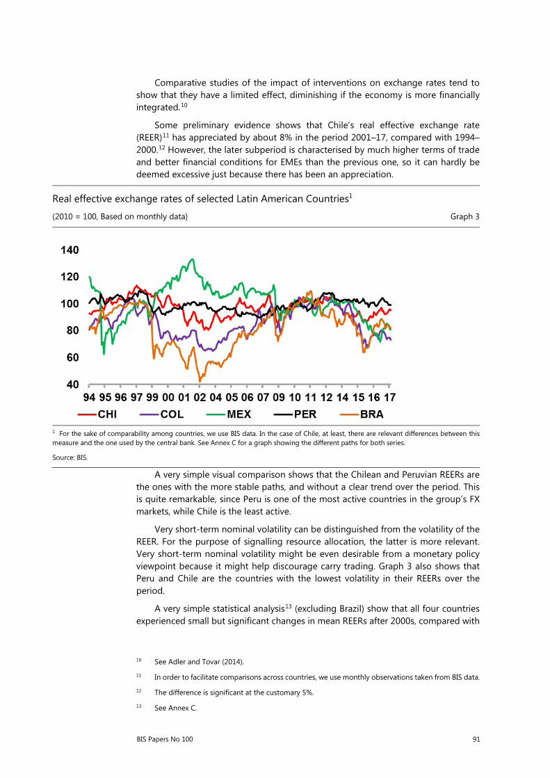
BIS Papers No 100 91
Comparative studies of the impact of interventions on exchange rates tend to show that they have a limited effect, diminishing if the economy is more financially integrated.10
Some preliminary evidence shows that Chile’s real effective exchange rate (REER)11 has appreciated by about 8% in the period 2001–17, compared with 1994–2000.12 However, the later subperiod is characterised by much higher terms of trade and better financial conditions for EMEs than the previous one, so it can hardly be deemed excessive just because there has been an appreciation.
Real effective exchange rates of selected Latin American Countries1
(2010 = 100, Based on monthly data) Graph 3
1 For the sake of comparability among countries, we use BIS data. In the case of Chile, at least, there are relevant differences between this measure and the one used by the central bank. See Annex C for a graph showing the different paths for both series.
Source: BIS.
A very simple visual comparison shows that the Chilean and Peruvian REERs are the ones with the more stable paths, and without a clear trend over the period. This is quite remarkable, since Peru is one of the most active countries in the group’s FX markets, while Chile is the least active.
Very short-term nominal volatility can be distinguished from the volatility of the REER. For the purpose of signalling resource allocation, the latter is more relevant. Very short-term nominal volatility might be even desirable from a monetary policy viewpoint because it might help discourage carry trading. Graph 3 also shows that Peru and Chile are the countries with the lowest volatility in their REERs over the period.
A very simple statistical analysis13 (excluding Brazil) show that all four countries experienced small but significant changes in mean REERs after 2000s, compared with
10 See Adler and Tovar (2014).
11 In order to facilitate comparisons across countries, we use monthly observations taken from BIS data.
12 The difference is significant at the customary 5%.
13 See Annex C.

92 BIS Papers No 100
the second half of the 1990s, something that could be explained by changing external conditions (terms of trade, financial access). More interesting, though, is the weaker evidence of changes in volatility in REERs in the second period, characterised by higher globalisation and generally more flexible nominal exchange rates. When we compare the volatility of the REER among countries in the 2001–17 period, variances were found to be higher for Colombia and Mexico than for Peru and Chile, with statistically significant differences between Colombia and Chile, and Colombia and Peru, but not between Chile and Peru.
Labour market globalisation: effects of immigration
Historically immigration has played a significant role in Chile’s development, with policies to attract (mostly European) migrants to settle in the southern part of the country in the second half of the nineteenth century. However, in the second half of the last century, there was a net emigration of Chileans. The number of foreign migrants into Chile remained at about 100,000 for most of this period. Starting in the mid-1990s, Chile began to attract a growing number of immigrants from Latin America, first from neighbouring countries (Peru and Argentina), and more recently, from Colombia, Venezuela and some Caribbean countries, notably Haiti. The common factor behind this new trend was better economic opportunities and, to some extent, political crisis and violence in the countries of origin. According to the most recent data, immigrants number about 450,000 people (about 2.6% of the population), mostly young and with high participation rates in the labour market. In terms of education, when we look at averages, immigrants have higher levels of schooling than the average Chilean, even though there are large differences depending somewhat on the countries of origin.14
So far there have been no signs of a backlash against immigration, but there is widespread support for the idea of refreshing legislation as well as to improving compliance with the relevant existing laws and regulation.
In terms of their economic contribution, immigrants have a very visible presence in services ranging from household help and other basic jobs to medical doctors, helping to fill a large number of vacancies in the public health services.15 From a macroeconomic point of view, a recent study by the central bank16 estimated that trend annual GDP growth for the next 10 years will be about 3.5%. The overall contribution of labour to that figure was 0.8% per year, of which a quarter (0.2% of GDP growth) would be due to immigration.
14 Cabieses and Bustos (2016).
15 Last year more than a third of doctors taking the annual qualification exams to practise their profession in Chile were foreigners.
16 Central Bank of Chile (2017) and the summary in the quarterly monetary policy report for September.

BIS Papers No 100 93
Effects of new barriers to global trade
As Chile is a small and open economy, it is vulnerable to the effects of new trade barriers. The main question then is by how much and through which channels.
Given that Chile exports mostly industrial raw materials and agro-forestry products,17 and that it has free trade agreements with all main partners, we consider it unlikely that the country might be subject to major trade sanctions.
However, the country might be vulnerable if trade sanctions are imposed on its major import partners. China is the most critical case. Even though there are estimates of the potential impact of trade sanctions on China’s economic growth, it would be difficult to estimate the effects on the specific markets that are relevant to Chile.
Another scenario that might have an impact on Chile’s competitiveness is the eventual taxation of the greenhouse gas (GHG) emissions of imports. We expect the GHG footprint of the Chilean economy to fall in the future as new-generation renewables and hydro displace coal and diesel in electric power generation. However, the long distance to markets would become a significant disadvantage if transportation emissions were to be taken into account. This is particularly the case with heavy bulk cargo, such as minerals, as well as for exports requiring refrigeration such as fresh fruits, vegetables and seafood.
Final comments
As Chile’s re-integration into the global economy was accompanied by major economic and institutional reforms, it is difficult to isolate the specific contribution of globalisation to the improved economic performance. It is worth noting that globalisation has not featured on the political agenda in recent years, even though there have been major controversies about topics such as pensions, labour regulations, environmental issues, wealth and income distribution and so forth. Even immigration has not produced as large a negative reaction as in other countries.
In terms of macroeconomic policies, there is widespread support for fiscal discipline, at least in principle and, if anything, for strengthening the fiscal rule. There is also wide support for the central bank’s independence. What is more controversial is the free flotation of the exchange rate, with strong calls from exporters’ organisations to intervene whenever the currency appreciates significantly. The evidence shown here suggests that these interventions make little difference in the evolution of the REER, while, in the case of Chile at least, they may result in a severe deterioration of the central bank balance sheet. As Chile is a small economy, globalisation has brought a significant measure of competition to many goods markets that were formerly protected, as well as better access to capital and intermediate goods, making a significant contribution to the overall increase in productivity.
17 Industrial inputs might receive political support from importing companies abroad, while agricultural
products are protected by nature, as the main markets are in the northern hemisphere with the opposite growing seasons.

94 BIS Papers No 100
The elimination of trade barriers has resulted in a major increase in exports and imports with a significant structural effect in terms of the composition of goods and services traded. Exports remain highly biased towards natural resources. Factors such as the size of the domestic market as well as the distance to large global markets continue to hinder full integration into global value chains. Improvements to infrastructure and trade process efficiency could help to mitigate these disadvantages.
Financial integration has helped to reduce significantly the country’s cost of capital, while providing pension funds with a valuable way of diversifying risk. Chile exhibits some of the largest measures of financial market depth among EMEs.
Finally, FDI has made a large contribution to the development of Chile’s productive capacity. In recent years, outward FDI, especially to the region, has helped to sustain major Chilean corporations, mostly in the service sector, to grow beyond the limits of the domestic markets.

BIS Papers No 100 95
References
Adler, G and C Tovar (2014): “Foreign exchange interventions and their impact on exchange rate levels”, Monetaria, January–June, CEMLA.
Arellano, J (2006): “Del déficit al superávit fiscal: razones para una transformación estructural en Chile”, CIEPLAN.
Central Bank of Chile (2017): “Crecimiento tendencial: proyección de mediano plazo y análisis de sus determinantes”, September.
Cabieses, B and P Bustos (2016): “Perfil socio-demográfico de migrantes internacionales en Chile” in B Cabieses, M Bernales and A McIntyre (eds), La migración internacional como determinante social de la salud en Chile: evidencia y propuestas para políticas públicas, Programa de Estudios Sociales en Salud, Universidad del Desarrollo.
Collier, S and W Sater (1996): A History of Chile, 1808–1994, Oxford University Press.
Dornbusch, R and S Edwards (1991): The Macroeconomics of Populism in Latin America, University of Chicago Press.
Ffrench-Davis, R (1973): Políticas económicas en Chile 1952–1970, CEPLAN, Ediciones Nueva Universidad.
——— (2010): Economic reforms in Chile. From dictatorship to democracy, Palgrave Macmillan.
Figueroa, E, G Donoso, G Lagos, G Alvarez and J Muñoz (1996): “Sustentabilidad ambiental del sector exportador chileno”, in O Sunkel (ed), Sustentabilidad ambiental del crecimiento económico chileno, Universidad de Chile.
Larraín, F and R Vergara (2000): La transformación económica de Chile, Centro de Estudios Públicos.
Meller, P (1996): “El modelo exportador chileno. Crecimiento y equidad”, CIEPLAN.
——— (1998): “Un siglo de economía política Chilena (1890-1990)”, CIEPLAN.
Naudon, A and J Vial (2016): “The evolution of inflation in Chile since 2000”, BIS Papers, no 89.
Schmidt-Hebbel, K (2006): “Chile’s economic growth”, Cuadernos de Economía, vol 43, May.
Thorp, R (1998): “Progreso, Pobreza y Exclusión. Una historia económica de América Latina en el Siglo XX”, IADB.
Vegh, C and G Vulletin (2014): “The road to redemption: Policy responses to crisis in Latin America”, NBER Working Papers, no 20675.
World Bank (1994): “Managing environmental problems: Economic analysis of selected issues”, Report, no 13061-CH.

96 BIS Papers No 100
Annex
Indicators of structural changes and performance of the Chilean economy during the re-integration into the world economy Annex A1
Sources: Central Bank of Chile; World Bank.
Average annual flows of foreign direct investment
(percent of GDP) Annex A2
Sources: Central Bank of Chile; World Bank.
0
10
20
30
1971-1989 1990-2005 2006-2016
Chile imports by origin(percent of GDP)
United States Japan ChinaOther Asia Europe Other
0
10
20
30
40
1971-1989 1990-2005 2006-2016
Chile exports by destination(percent of GDP)
United States Japan ChinaOther Asia Europe Other
0
2
4
6
8
10
1984-1989 1990-2005 2006-2016Outflows Inflows

BIS Papers No 100 97
Composition of exports
(percent of GDP) Annex A3
Source: Central Bank of Chile.
Average inflation rate for Chile
(year on year) Annex A4
Sources: Central Bank of Chile; National Institute of Statistics (INE).
0
10
20
30
40
1970 2014Mining and processed Forestry and manufactured products from forestryFresh, frozen and processed fruit Fresh, and processed sea productsWine MeatRest of manufactures
0
20
40
60
80
100
120
1971-1989 1990-2005 2006-2016

98 BIS Papers No 100
Average GDP growth
(year on year) Annex A5
Source: Central Bank of Chile.
0.0
1.0
2.0
3.0
4.0
5.0
6.0
1971-1989 1990-2005 2006-2016

BIS Papers No 100 99
Relative importance of imports in local consumption of selected goods Annex B
Sources: Central Bank of Chile; I-O matrices (INE).
Trends and volatility of exchange rates in selected countries (1995–2017) Annex C
Descriptive statistics Period I: 1994–2000; Period II: 2001–October 2017
Statistical Test 1, Comparison between periods, same country Period I: 1994–2000; Period II: 2001–October 2017
Note: ** means that Null Hypothesis is rejected with 95% confidence. * reflects the same with 90% confidence. T statistics show the result of the mean differences between periods, with the null hypothesis of equal means. F statistics show the result of variance differences between periods, with the null hypothesis of equal variance.
Sources: Bloomberg; BIS.
Table 1. Imported origin as a fraction of total expenditure in selected items (%)
1986 1996 2003 2008 2013Clothing 13% 27% 51% 64% 73%Footwear 2% 24% 48% 61% 78%Household appliances 73% 93% 97% 81% 89%Automobiles 100% 100%
Selected imports as % GDP 5,5% 6,0% 7,5% 7,3% 12,3%
I II I II I II I IIMean 453 579 1321 2315 7.7 12.7 2.8 3.1Standard deviation 54 79 451 421 2.1 2.7 0.5 0.3N° observations 84 202 84 202 84 202 84 202Mean 103.0 94.7 88.5 84.9 98.2 102.9 101.54 98.613Standard deviation 5.4 6.0 8.5 11.8 14.6 12.7 5.02 4.34N° observations 84 202 84 202 84 202 84 202
Chile Colombia México Perú
Nominal exchange rate
Real Exchange rate (BIS)
I II I II I II I II
Mean difference (t statistic)
Variance difference (F statistic)
Mean difference (t statistic)
Variance difference (F statistic) 0.798 0.51** 1.32* 1.38*
Real Exchange rate (BIS)
Chile Colombia México Perú
Nominal exchange rate
11.37** 2.87** -2.54** 4.66**
-15.6** -17.31** -16.92** -6.11**
0.46** 1.14 0.57** 2.73**

100 BIS Papers No 100
Trends and volatility of exchange rates in selected countries (1995–2017)
Annex C
(continued)
Statistical Test 2, Differences in REER volatility among countries over the 2001–17 period Variance difference tests, Chile’s REER versus other Latin American countries:
Test Colombia Mexico (*) Peru Value Prob. Value Prob. Value Prob.
F-test 3.8 0.00 4.4 0.00 1.94 0.000 Siegel-Tukey 7.7 0.00 6.2 0.00 3.40 0.001 Bartlett 84.7 0.00 102.1 0.00 21.52 0.000 Levene 131.9 0.00 62.2 0.00 24.18 0.000 Brown-Forsythe 96.2 0.00 61.6 0.00 24.14 0.000
Different measures of real effective exchange rates for Chile (BIS and Central Bank of Chile)
(*) Tests results for Mexico are included for completeness but they should be disregarded because the REER for Mexico is not stationary over this period.
Sources: Central Bank of Chile; BIS.
70
90
110
130
94 96 98 00 02 04 06 08 10 12 14 16
REER(2010=100, Based in monthly data)
REER CBCh REER BIS

BIS Papers No 100 101
How globalisation has affected China and related policy issues
The People’s Bank of China
Abstract
Globalisation is a double-edged sword, especially for EMEs. On the one hand, globalisation has boosted national income, spurred trade and investment and promoted the sustained and healthy development of China’s economy. On the other hand, globalisation has also expanded China’s domestic income gap and intensified pressure on cross-border capital flows. As a response to these challenges, and like other EMEs, China conducts sound macroeconomic policies and promotes structural reforms with the aim of creating a robust macroeconomic environment.
Keywords: globalisation, China's economy, reform.
JEL classification: F60.
102 BIS Papers No 100
Implications for output, trade and investment in China
Globalisation has promoted the sustained and healthy development of China’s economy and China has also injected new impetus into globalisation. Especially after China’s WTO accession, the adoption of advanced technologies and management expertise, external competition and technological innovation have enhanced China’s total factor productivity and economic growth. GDP expanded from USD 189 billion in 1980 to USD 12.2 trillion in 2017, accounting for 15% of global GDP. While benefiting from globalisation, China has also contributed significantly to global growth. Between 2012 and 2016, China contributed over 30% to the global economic growth on an average annual basis. Globalisation also promoted a synchronised uptick in China’s output and the global economic cycle, but it also aggravated the impact of external shocks, as in the Asian financial crisis in 1997 and the Great Financial Crisis in 2007–09. The Chinese economy has been resilient to external shocks thanks to reforms, economic opening and new growth drivers.
Globalisation has spurred trade and investment, intensifying pressure on cross-border capital flows. Since the reforms and economic opening, China’s external trade has surged. In 2017, the total volume of imports and exports exceeded USD 4 trillion, compared with less than USD 40 billion in 1980. Meanwhile, China has cumulatively attracted over USD 1.7 trillion of foreign investment and made a total of USD 1.2 trillion of outward direct investment. Globalisation has intensified the pressure of cross-border capital flows. After China joined the WTO in 2001, the scale of cross-border capital flows continued to increase. Later, with the shift of monetary policy stance in the major advanced economies, international capital began to flow out of China, reaching USD 6.1 trillion in 2016, 13 times that of the 1997 Asian crisis. Short-term capital flows accounted for nearly 60% of this. The leverage ratio of Chinese enterprises increased from 96% in 2006 to 144% in 2016, higher than that not only of advanced economies such as the United States (72.8%) and Japan (94.2%) but also of some EMEs such as Korea (103.7%).
Implications for population flows and income distribution: globalisation has promoted labour flexibility and geographic mobility in China.
Migration has been growing in the past 30 years, especially after China’s WTO accession in 2001. By 2016, domestic population flows had reached 245 million. During this period, economic restructuring and rapid industrialisation supported a boom in labour-intensive industries in the coastal region. Migrant workers have moved from rural to urban areas, and from underdeveloped to developed areas. China’s per capita income has risen substantially in this process. Moreover, China has gradually evolved from a country of emigrants to being both a source of emigration and a country for immigration. In addition, China has facilitated the international flow of labour by simplifying its visa procedures.
Globalisation has boosted national income but also expanded the domestic income gap. With the reforms, economic opening and continuous integration into

BIS Papers No 100 103
the global economy, China has grown at a remarkable pace. A massive amount of people have been lifted from poverty. The rural poor population has dropped from 98.99 million in 2012 to 43.35 million in 2016. The quality of life has improved significantly. Per capita disposable income reached CNY 25,974 in 2017, 2.1 times that of 2010. However, the income gap has also expanded. The Gini coefficient rose from 0.292 in 1981 to the peak of 0.491 in 2008, before declining slightly to 0.465 in 2016, above the internationally acknowledged appropriate level of 0.4. Wealth gaps exist between urban and rural areas, as well as between different regions and industries.
Discrepancies in the progress of reforms, the shift of economic activities to coastal areas and monopolies in certain industries have contributed to such gaps. According to estimates, the Gini coefficients of urban and rural areas rose from 0.172 and 0.256 in 1981 to 0.326 and 0.376 respectively in 2014. From 2005 to 2014, the average income of the top quintile in Beijing was four times as much as that of the bottom quintile. Income gaps between senior management and ordinary staff yawn in the monopoly industries, especially the telecommunications and petroleum industries.
Policy issues
Globalisation is a double-edged sword, especially for EMEs. Like other emerging market economies, China has responded with sound macroeconomic policy and structural reforms to create a good domestic environment for participating in globalisation.
First, we are adapting to the new normal of economic development and deepening supply side structural reforms. We actively promote the reform of state-owned enterprises, and we are adjusting industrial structures, and eliminating overcapacity and “zombie” enterprises. We have sought to encourage technological innovation, increase investment in education, and improve labour quality and total factor productivity. We aim to cut costs for enterprises, reduce real estate inventory through tax measures, land and resource price reforms, and to reform the administrative system by streamlining administration and delegating powers.
Second, we are implementing precise poverty relief measures and increasing financial assistance to the agricultural sector and farmers. We will leverage fiscal policy to adjust income distribution, integrate agriculture-related fiscal funds through various channels, actively improve poverty relief and development policy, strengthen supervision of capital and projects, and improve the infrastructure and basic public services in poor areas. We aim to achieve the goal of reducing the rural poverty population by 10 million this year.
Third, we are strengthening the macroprudential management framework of the financial sector and coordinating monetary policy with macroprudential management. In particular, we will strengthen macroprudential management of cross-border capital flows and regulate risk reserves for forward sale of foreign exchange in a flexible manner. This will ensure that cross-border financing is consistent with macroeconomic conditions, overall solvency, and the balance of payments position, with a view to creating a stable macro environment for economic development.

104 BIS Papers No 100
Last but not least, we will further open up the financial industry. We will actively promote the Belt and Road Initiative and explore new paths for opening up the financial industry. We will implement comprehensive financial sector reforms and enhance the competitiveness and soundness of financial institutions. We aim to restore the profitability of the financial sector to an appropriate level and reduce the wealth gap within the financial industry through greater competition. We will also improve financial services and mitigate overall financial risks.

BIS Papers No 100 105
International trade networks and the integration of Colombia into global trade
Andrés Murcia, Hernando Vargas and Carlos León1
Abstract
Global trading activity for different types of goods is mapped using network analysis, comparing the mid-1990s with recent years. Variations in trade patterns through time are described and the rise of new players in different sectors is documented. Subsequently, some features of the integration of Colombia into global trade are presented along with some evidence on the impact of this process on the responsiveness of the manufacturing sector to exchange rate shocks. The main conclusions are the following: (i) globalisation has generated important changes in international trade, increasing the links between countries and making the world trade network (WTN) denser, more reciprocal and more clustered; (ii) the rise of China in global trade is perhaps one of the most important developments in recent years; (iii) nevertheless, this process has been uneven across sectors; (iv) the integration of the Colombian economy into global trade has been significant but imperfect; and (iv) the exposure of Colombian manufacturing firms to international markets on both their demand and cost sides may be an important reason why manufacturing output and trade have not responded much to fluctuations in exchange rates.
Keywords: international trade, network analysis, globalisation, manufacturing sector, real exchange rate, Colombia.
JEL classification: F15, F60, F31.
1 Head of International Affairs, Technical Deputy Governor and Senior Researcher at Financial Market
Infrastructure Oversight Department at Bank of the Republic, Colombia, respectively. The opinions contained herein are the sole responsibility of the authors and do not necessarily reflect those of Bank of the Republic or its Board of Directors. All errors and omissions remain our own. We are grateful to Enrique Montes, Juan Esteban Carranza, Camila Casas and Angie Rozada for their contributions.
106 BIS Papers No 100
1. Introduction
Since the end of the eighties and the beginning of the nineties, the Colombian economy went through a process of economic opening that sought to further integrate the country into global trade. To illustrate the international environment in which this process took place, the next section of this note uses network analysis to map global trading activity for different types of goods. Variations in trade patterns through time are described and the rise of new players in different sectors is documented. The third section then highlights some specific features of the integration of Colombia into global trade. Some evidence about the impact of this process on the responsiveness of the manufacturing sector to exchange rate shocks is examined in the fourth section.
The analysis presented in this note is based on previous work by the staff of Bank of the Republic, some of which has been published in the Bank’s working paper series.
2. The world trade network
Cepeda et al (2017) describe the evolution of the world trade network (WTN) from the mid-1990s to 2014. Using network analysis, the authors find that countries’ efforts to attain the benefits of trade have resulted in a trade network that is increasingly dense,2 reciprocal3 and clustered,4 suggesting that globalisation has resulted in a larger number of trade relations. However, they found no sizeable effect on their intensity. Hence, trade linkages are homogenously distributed among countries, but their intensity is highly concentrated in few of them.
The study used the United Nations Comtrade Database for the period 1995– 2014, for the 106 countries reported in the database that are the main constituents of the WTN.5 The authors concluded that the value of exports was concentrated on just a few countries during the whole sample period and that 2007–08 marked a turning point in the WTN’s evolution from a two-strong group (led by United States and Germany) to a three-strong group (led by United States, Germany and China), forming a hierarchical structure of world trade. Although these countries preside over the most intense trade flows, the links between countries appear to be distributed homogeneously among them. In other words, the WTN is a very dense network that consists of a large number of countries with multiple weak trade relations, and a small set of countries with multiple and intense relations. The authors argue that gravity models (eg Tinbergen (1962)) could explain some important features of global trade, since the proximity of countries in the trade network tends to be associated with
2 Density is the ratio of the number of actual links to the maximum possible number of links.
3 Reciprocity measures the probability that a link from country “i” to “j” is complemented by the reciprocal link, from “j” to “i”.
4 Clustering measures the frequency with which loops of tree lengths appear in the network.
5 Export measures were included for the following sectors: animal and animal products; vegetable products; foodstuffs; mineral products; chemicals and allied industries; plastics and rubbers; raw hides, skins, leather and furs; wood and wood products; textiles; footwear and headgear; stone and glass; metals; machinery and electrical; transportation; miscellaneous; and other (services).
BIS Papers No 100 107
characteristics such as the size of the economies and their geographical location. Nevertheless, some recent changes in the WTN may have to do with a changing pattern in specialisation in global trade, whereby China’s rise as a manufacturing exporter has concentrated exports of some countries in raw material sectors. In this process China’s emergence has disrupted manufacturing output and exports in many countries, increasing global demand for raw materials.
Cepeda et al (2017) also found that the characteristics of the WTN (density, reciprocity, clustering etc) cannot be understood as the average of the features of the sectoral trade networks. In addition, since globalisation and technological spillovers affect sectors and economic activities in different ways, it is especially relevant to analyse whether there have been differences in the evolution of sectoral trade networks. In this note, we try to go deeper into the analysis in this regard.6 We report sectoral networks and minimal spanning trees7 to illustrate the evolution of five components of the WTN – vegetables, minerals, metals, machinery and electrical, and transportation. This yields a clear picture of the differences between the WTN of commodities and high-value added products in the periods 1995–96 and 2013–14.
The sectoral networks used to analyse the evolution of the WTN (Graph 1) are interpreted as follows: the red nodes correspond to countries that pertain to the 90th percentile of exports, and the diameter of each one is the country’s contribution to the value of total exports in the respective sector for each period. They are positioned in a circular layout, where the most representative country (by value of exports) is at the rightmost location, and those that follow are positioned in descending counterclockwise order. The links between countries are represented by arrows that follow the direction from exporter to importer, whereas their width and colour (see colour scale on the left) represent their contribution to the total value of exports.
After a simple visual inspection of the sectoral networks (Graph 1) and their respective minimal spanning trees (Graph 2), it is possible to observe that: (i) there are more links between countries in the second period (2013–14) than in the first one (1995–96), suggesting that globalisation has increased trade relations between countries in the last 20 years; (ii) the number of countries in the network in the first three sectors (vegetables, minerals and metals) is larger than in the other two sectors (machinery/electrical and transport), indicating a higher concentration in those sectors with greater value added; (iii) the emergence of new relevant players in most sectors is evident. The salient case is China, which was a satellite node linked to other countries in many sectors in the 1990s, but has become one of the principal nodes 20 years later; and (iv) regional trading blocs are quite relevant.
We now present some results of the visual inspection for different sectors (Graphs 1 and 2) and the evolution of the main network metrics (presented in Graphs 3, 4, 5 and 6).
6 A similar exercise was performed by Cingolani et al (2017) for the sectors of textiles and electronics.
For the mining sector Zhong et al (2017) also use network analysis.
7 Minimal spanning trees consist of choosing the shortest distances of a connected system of n countries in such a way that the resulting system is an acyclic network with n–1 links.

108 BIS Papers No 100
Vegetables.8 This is probably the sectoral network with fewest changes during the period studied. The principal nodes in the 1990s were the United States, the Netherlands, Germany and, to some degree, China. For the second period, the most relevant nodes are the same, but China gained importance and India became relevant as well (Graphs 1 and 2). In South America, countries with large agricultural sectors, such as Argentina and Brazil, changed their leading trade link from the United States to China. Based on the summary network statistics (Graphs 3, 4, 5 and 6), it is remarkable that this sector shows the lowest reduction in the average geodesic distance9 between countries, suggesting that this sector experienced relatively fewer changes in trade patterns. It is also noteworthy that this sector is the only one that presents a reduction in the reciprocity measure and exhibits the lowest change in clustering degree. The role of specialisation in this sector and the difficulty of changing production patterns could be part of the explanation.
Minerals.10 The most relevant nodes in this network during the 1990s were the United States, Japan and Saudi Arabia and, to a lesser degree, Norway, the Netherlands, Russia and the United Kingdom. Looking at the network of 2013–14, the emergence of China is again noticeable. Also, countries such as Russia and Australia increased their importance in the global minerals trade network. The increase in the density measure of this network has been similar to that of other sectors during the last two decades (Graph 4), suggesting an augmented trading activity with new country destinations. Despite the increase in new trading relations, growth in the measures of reciprocity and clustering has been relatively low. This can be expected in commodity goods sectors such as minerals, given the limited number of country participants in the production chain.
Metals.11 The evolution of this network mimics that of total international trade (WTN). In the 1990s, trade was dominated by the United States, Germany and Japan. Twenty years later, the most relevant players were China, Germany and, to a lesser degree, the United States. In Latin America, big producers of copper and other minerals, such as Chile, changed their main counterparty from the United States to China during that period. The United States kept an important role through its links with regional partners such as Canada and Mexico. The network statistics suggest that trade links have multiplied during the period analysed: the average distance decreased, while the density, reciprocity and clustering measures increased.
8 The vegetables group includes live trees and other plants; edible vegetables and certain roots and
tubers; edible fruit and nuts; coffee, tea, mate and spices; cereals; products of the milling industry; oil seeds and oleaginous fruits; gums, resins and other vegetable saps; vegetable plaiting materials and animal or vegetable fats and oils.
9 Average geodesic distance is the average of the shortest path in term of number of links from country i to j.
10 The minerals group includes salt, sulphur, earths and stone; ores, slag and ash, and; mineral fuels and oils.
11 The metals group includes iron and steel; article or iron or steel; copper; nickel; aluminum; lead; zinc; tin, other base metals; tools, implements, cutlery, spoons and forks and; miscellaneous articles of base metal.

BIS Papers No 100 109
Machinery/electrical12 and transport.13 These categories include goods whose production processes are characterised by greater complexity and heavier reliance on technology. Trade in machinery and electrical goods was concentrated in the United States and Germany in the 1990s, whereas in 2013–14 China became an important player, taking the place of the United States in the world trade network of these goods. For the transport sector the biggest nodes remained the same (the United States and Germany), but new relevant players had emerged in 2013–14 (eg Brazil, Sweden and India). Mexico’s weight in this network increased markedly and its trade link with the United States is today one of the largest trade relations worldwide (purple line in Graph 1).
Both machinery/electrical and transport networks have recorded increases in their density, reciprocity and clustering measures, as well as significant reductions in the average distance between countries, suggesting that trade links have been substantially enhanced. This may reflect the greater importance of multinational companies in these activities and the extension of global value chains (GVC).
According to BIS (2017), between 1995 and 2007, the ratio of trade in intermediate to final goods and services rose from 1.25 to 1.75. GVCs alter production processes and international links between countries in different ways. In particular, GVCs allow the substitution of foreign production inputs for domestic ones in a flexible manner (BIS (2017)). By shifting production stages geographically and across plants, firms can exploit efficiency gains on a global scale and bypass domestic constraints or bottlenecks. GVCs also include long-term economic relationships between unaffiliated firms that buy and sell inputs specialised for each other’s needs (Antràs (2005)). The rise of China can also be seen through the change in GVCs. According to BIS (2017), the share of China in the global trade of intermediate goods and services surged from just 2.2% in 1995 to no less than 9.1% in 2014.
3. The integration of Colombia into global trade
In the beginning of the 1990s, the country undertook a series of structural reforms in order to increase productivity and efficiency. The liberalisation of the foreign trade regime was an important component of this effort. Tariffs were reduced and some quantitative import restrictions were eliminated. The simple average nominal tariff on imports was reduced from 31% to 17% between 1985 and 1992, and to 12% between 1992 and 1997. In 2015, the average tariff on imports was 5.8%.
Despite a significant increase in the value of imports and exports between 1990 and 2015 (Graph 7), the integration of the Colombian economy into global trade has been incomplete and imperfect. The evolution of a common trade openness
12 The machinery and electrical group includes nuclear reactors, boilers, machinery and mechanical and
electrical machinery and equipment.
13 The transportation group includes railway or tramway locomotives, rolling-stock, vehicle other than railways or tramways; aircraft, spacecraft and parts, and; ships, boats and floating structures.

110 BIS Papers No 100
indicator14 suggests that Colombia is still closed relative to other countries in the region (Graph 8). Additionally, an increasing part of export trade corresponds to mining and energy commodities, resulting in high levels of concentration in these sectors (Graph 9, red line). This is also evident in the evolution of a Herfindahl concentration indicator (HHI) calculated for categories in the Colombian exports15 (Graph 9, green line), while diversification by country of destination has recorded some gains (Graph 9, blue line). Based on micro level information, Eaton et al (2007) noticed that export sales have been dominated by a small number of very large and stable exporting firms, suggesting a high firm-level of concentration in the export market.
As for imports, it should be noted that the variety of products imported by the country has been reduced.16 All this suggests that gains in terms of diversification of markets in this period have been limited.
This pattern is partially explained by the fact that the reduction in tariffs was accompanied by the imposition of other measures with protectionist effects. Although the average tariff fell and the quantitative control of imports was abandoned, the use of non-tariff measures became widespread (García et al (2014)). Since 1991, there has been a steady increase in decrees, regulations and resolutions for technical standards as well as sanitary measures intended to protect consumers or producers, which has resulted in higher prices for consumers and increased protection for producers (García et al (2015A)).
The quality of institutions has also hindered the process of international integration. A central bank survey of logistics operators in early 2013 suggests that regulatory agencies are seldom coordinated and that regulations constitute a barrier to trade because they are opaque, complicated and not disclosed in a timely manner (García et al (2015 B)). Moreover, trade policy in Colombia is defined and executed by several entities (currently more than 20), unlike the period prior to the economic opening, when it was defined and executed by just a few. The present organisational structure has added barriers to foreign trade through the entities’ requirements for approval or for giving a favourable concept of imports or exports. All these problems may pose a barrier to trade and tend to reduce its volume significantly (García et al (2015B)). The above-mentioned survey also found high internal non-tariff costs, particularly those relating to internal transport of cargo, port services, agency services, inspections by some sanitary entities other than customs, and prior authorisations. All this suggests that the integration of Colombia into the global economy has been limited and imperfect, and that there is still quite significant room for improvement.
14 Calculated as the ratio of the sum of exports plus imports to GDP. 15 This indicator is defined as the sum of the squares of the participation of each category of exports
within the total exports (as a measure of market share). Increases in the HHI indicator generally indicate an increase in concentration. We used 180 categories of exports according to the International Standard Industrial Classification of All Economic Activities (ISIC) Rev. 3.
16 In 1995, Colombia imported goods that corresponded to 6,790 positions of the customs tariffs; in 2015, the number of positions had fallen to 6,459.

BIS Papers No 100 111
4. Manufacturing sector and its responsiveness to exchange rate shocks
Despite the above-mentioned obstacles, a salient feature of the manufacturing sector during the last two decades has been its increased exposure to international trade, thanks to the growing globalisation of its input and output markets. The fact that the manufacturing sector is exposed to exchange rate fluctuations that affect both its demand and its costs has served to mitigate the effects of these shocks. Based on González et al (2017), we present here some insights into how the fluctuations of the exchange rate have affected the Colombian manufacturing sector since 2000 and how globalisation has affected the link between these variables. Recent evidence suggests that, in the context of multi-country production chains, third-country exchange rate effects could generate “complementarities” between real effective exchange rates (BIS (2017)), in the sense that the competitiveness of a home exporting firm that sources heavily from a third country could be affected by changes in the exchange rate of that country.17 According to BIS (2017), novel quantifications of real exchange rate dynamics in the presence of international input-output linkages find that the magnitude of such effects is material (Bems and Johnson (2016), Patel et al (2014)).
Manufacturing output and exports grew steadily in Colombia until the 2008–09 international financial crisis, when worldwide manufacturing and trade slowed significantly (Graph 10). After 2010, growth in manufacturing output held up, despite the real appreciation of the currency18 of around 20% between 2001 and 2012. In fact, if anything, manufacturing output and exports seem to be positively correlated with the real exchange rate. Moreover, after the substantial depreciation of the currency after 2014, manufacturing output has not picked up significantly (Graph 10).
The resilience of manufacturing to the fluctuations of the exchange rate is partly explained by confounding factors that affect both, such as the strength of external and internal demand. Furthermore, in an increasingly globalised economy, firms that produce tradable goods using tradable inputs are exposed to exchange rate shocks in both their final goods markets and their input markets. These effects may offset each other, especially if they differentially affect the currencies of the countries from
17 BIS (2017) presents an example to explain the complementarity of real effective exchange rates: “As
German firms source heavily from China, the competitiveness of German producers exporting to France improves if the renminbi devalues against the euro”. The authors also claim that “The third-country effects present in GVC-based REERs work in opposite directions to those present in traditional final goods-based REERs. This is because final goods from third nations substitute for domestic exports, whereas input goods sourced from third nations complement domestic production.”
18 The real exchange rate is measured as the ratio of the price of local goods to the price of foreign goods, so that an appreciation of the real exchange rate is equivalent to an increase of the index. To compute the real exchange rate index, let ERc=(ecP)/Pc be the bilateral real exchange rate with country c, where (ec/Pc) is the nominal exchange rate ec (units of c currency per Colombian peso) with country c divided by country c consumer price index Pc. The real exchange rate index ER is the sum of the bilateral real exchange rates with every trading country, weighted by their trading shares ER=∑csc(ecP)/Pc, where the shares sum up to one ∑csc=1 and depend on the type of goods that we look at.

112 BIS Papers No 100
where inputs are sourced and the currencies of the countries where goods are exported.
To illustrate this point, in Graph 11 we present a computation by González et al (2017) in which they discriminate real exchange rate indices for manufacturing exports and for inputs imported by manufacturing firms. Each index is based on the country shares of trade for each type of good. As shown, the cumulative appreciation of the real exchange rate is larger for imported inputs (blue line) than for exported manufactured goods (green line). Between 2000 and 2014, the real exchange rate of manufacturing exports increased, but the real exchange rate of manufacturing inputs rose even more. Between 2001 and 2012, the real appreciation of exports was around 17%, whereas the real appreciation of input imports was more than 25%.
In other words, there is evidence that, between 2000 and 2014, manufacturing firms hedged the effects of exchange rate shocks by importing inputs disproportionally from countries with relatively undervalued currencies (such as China and the United States), while disproportionally exporting to countries with relatively overvalued exchange rates (such as other Latin American countries). As presented in González et al (2017), this result is probably not a coincidence but, to some extent, an equilibrium result. For example, increased input imports from China might be the result of firms looking for less expensive suppliers, or a consequence of increases in the productivity of Chinese input-producing firms. In a globalised environment, both types of shock should increasingly be reflected in the composition of supply chains and the portfolio of markets of manufacturing firms.
In order to further illustrate the offsetting effects of exchange rate fluctuations, González et al (2017) computed a net real exchange index for the Colombian manufacturing sector since 2001. This index is calculated as the difference between the real exchange rate (RER) of exports and input imports, accounting for the share of exports in total sales, and the share of imported inputs in total costs.19 This measure is analogous to a standard RER index, except that it accounts for the proportion of output that is sold in the local market, and the proportion of inputs that are sourced from foreign countries. In Graph 12, the yearly percentage change of two measures of the real exchange rate and the change in the net real exchange rate (net RER) are presented. The blue line depicts the change of the RER based on the composition by destination of the manufacturing exports, whereas the red line depicts the change of the RER based on the composition by origin of imports of inputs for the manufacturing sector. The green line represents the yearly percent change of this net RER.
As reported in González et al (2017), the variation of the net RER index is much more muted than the variation of the standard RER. The reason is that input imports provide a natural hedge for firms against exchange rate fluctuations. The index reports some episodes of a real exchange net appreciation up until 2012, and a real exchange rate net depreciation since 2014. It should be pointed out that this index is computed for the whole manufacturing sector and that there should certainly be variation across sectors. In any case, the average net depreciation faced by manufacturing firms since 2014 has been only around 1% per year, which is much
19 Changes in the net RER are defined as Σi ΔTCRi (wi - ci). TCRi is the CPI-based bilateral RER with country
i, wi is the share of exports to country i in total sales, and ci is the share of imported inputs from country i in total costs. Zero economic profits are assumed, so that total costs equal total sales and both are approximated by the gross output of the economy.

BIS Papers No 100 113
lower than the observed depreciation of the nominal exchange rate. This stability of the net RER explains, at least partly, the weak growth of Colombian manufacturing after the substantial depreciation of the nominal exchange rate after 2014.
5. Conclusion
Globalisation has generated important changes in international trade, increasing the links between countries and making the world trade network (WTN) denser, more reciprocal and more clustered. However, the network remains highly concentrated on relatively few countries in terms of export values (Cepeda et al (2017)). The rise of China as an important player in global trade is perhaps one of the most important developments in recent years. This process, however, has been uneven across sectors, as documented in this note. The experience of Colombia in the globalisation process suggests that (i) the integration of the Colombian economy into global trade has been significant but imperfect; (ii) the exposure of manufacturing firms to international markets both on their demand and cost sides may be an important reason why manufacturing output and trade have not responded much to fluctuations in exchange rates. As the international linkages of firms deepen, this resilience could become more robust.
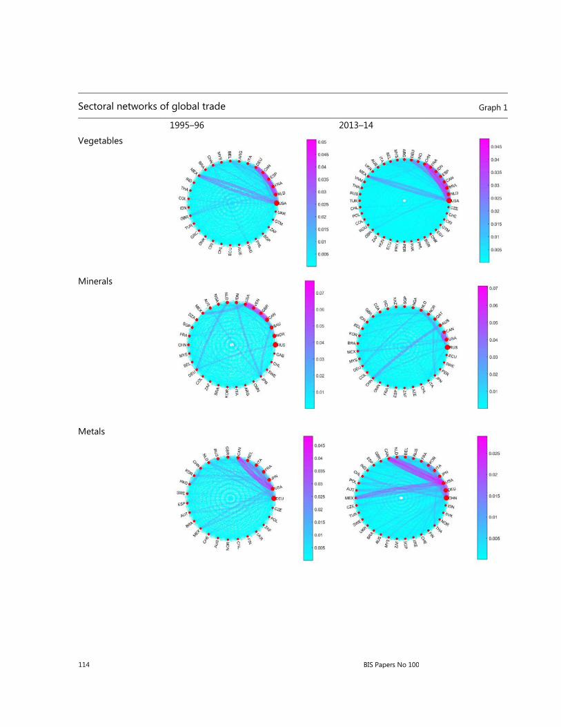
114 BIS Papers No 100
Sectoral networks of global trade Graph 1
1995–96 2013–14
Vegetables
Minerals
Metals

115
Machinery & Elect.
Transport
Source: UN-COMTRADE and Cepeda et al (2017), calculations by Bank of the Republic.

116 BIS Papers No 100
Minimal spanning trees of global trade Graph 2
1995–96 2013–14
Vegetables
Minerals
Metals
Source: UN-COMTRADE and Cepeda et al (2017), calculations by Bank of the Republic.

117
Minimal spanning trees of global trade Graph 2 (con’t)
1995–96 2013-14 Machinery & Elect.
Transport
Source: UN-COMTRADE and Cepeda et al (2017), calculations by Bank of the Republic.

118 BIS Papers No 100
Change in average distance in global trade between 1995–96 and 2013–14 Graph 3
Source: UN-COMTRADE and Cepeda et al (2017), calculations by Bank of the Republic.
Change in density in global trade between 1995–96 and 2013–14 Graph 4
Source: UN-COMTRADE and Cepeda et al (2017), calculations by Bank of the Republic.
-14.0%
-12.0%
-10.0%
-8.0%
-6.0%
-4.0%
-2.0%
0.0%
Machinery &Elect.
Transportation Metals Minerals Vegetables
Varia
tion
(199
5-96
vs.
201
3-14
)
0.0%
2.0%
4.0%
6.0%
8.0%
10.0%
12.0%
14.0%
16.0%
18.0%
20.0%
Machinery &Elect.
Transportation Metals Minerals Vegetables
Varia
tion
(199
5-96
vs.
201
3-14
)

119
Change in reciprocity in global trade between 1995–96 and 2013–14 Graph 5
Source: UN-COMTRADE and Cepeda et al (2017), calculations by Bank of the Republic.
Change in clustering in global trade between 1995–96 and 2013–14 Graph 6
Source: UN-COMTRADE and Cepeda et al (2017), calculations by Bank of the Republic.
-2.0%
-1.0%
0.0%
1.0%
2.0%
3.0%
4.0%
5.0%
6.0%
7.0%
8.0%
Machinery &Elect.
Transportation Metals Minerals Vegetables
Varia
tion
(199
5-96
vs.
201
3-14
)
0.0%
2.0%
4.0%
6.0%
8.0%
10.0%
12.0%
Machinery &Elect.
Transportation Metals Minerals Vegetables
Varia
tion
(199
5-96
vs.
201
3-14
)
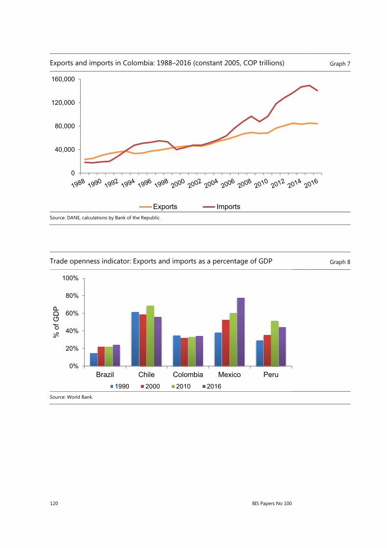
120 BIS Papers No 100
Exports and imports in Colombia: 1988–2016 (constant 2005, COP trillions) Graph 7
Source: DANE, calculations by Bank of the Republic.
Trade openness indicator: Exports and imports as a percentage of GDP Graph 8
Source: World Bank.
0
40,000
80,000
120,000
160,000
Exports Imports
0%
20%
40%
60%
80%
100%
Brazil Chile Colombia Mexico Peru
% o
f GD
P
1990 2000 2010 2016

121
Mining and oil exports as a percentage of total exports and Herfindahl concentration indicator for exports and trade partners, Colombia: 1992–2016 Graph 9
Sources: DANE, calculations by Bank of the Republic.
Manufacturing output, exports and real exchange rate in Colombia, 2001–16 Graph 10
Note: Data include all manufacturing sectors, excluding oil refining.
Sources: DANE, DIAN, calculations by Bank of the Republic.
0.0%
17.5%
35.0%
52.5%
70.0%
87.5%
0.
0.075
0.15
0.225
0.3
1992 1994 1996 1998 2000 2002 2004 2006 2008 2010 2012 2014 2016
% o
f tot
al e
xpor
ts
HHI for trade partnersHHI for exportsMining and oil exports (right axis)
60
70
80
90
100
110
120
130
50
100
150
200
250
300
2001
2002
2003
2004
2005
2006
2007
2008
2009
2010
2011
2012
2013
2014
2015
2016
2001
=100
Gross manufacturing outputExports (USD)Real exchange rate (manufacturing trade) Right axis

122 BIS Papers No 100
Manufacturing exports and input imports-based real exchange rate, 2001–16 Graph 11
Note: Data include all manufacturing sectors, excluding oil refining.
Sources: DANE, DIAN, Gonzalez et al (2017) calculations by Bank of the Republic.
Annual changes in real exchange rates in Colombia, 2001–16 Graph 12
Note: Changes in the net RER are defined as Σi ΔTCRi (wi - ci). TCRi is the CPI-based bilateral RER with country i, wi is the share of exports to country i in total sales, and ci is the share of imported inputs from country i in total costs. Zero economic profits are assumed, so that total costs equal total sales and both are approximated by the gross output of the economy.
Sources: DANE, DIAN, Gonzalez et al (2017) calculations by Bank of the Republic
50
60
70
80
90
100
110
120
130
140
2001 2002 2003 2004 2005 2006 2007 2008 2009 2010 2011 2012 2013 2014 2015 2016
Export-based RER input imports-based RER
-25%-20%-15%-10%-5%0%5%
10%15%20%
2001
2002
2003
2004
2005
2006
2007
2008
2009
2010
2011
2012
2013
2014
2015
2016
Change of the RER based on the composition by destination of themanufacturing exportsChange of the RER based on the composition by origin of imports ofinputs for the manufacturing sectorYearly percentage change of the net RER
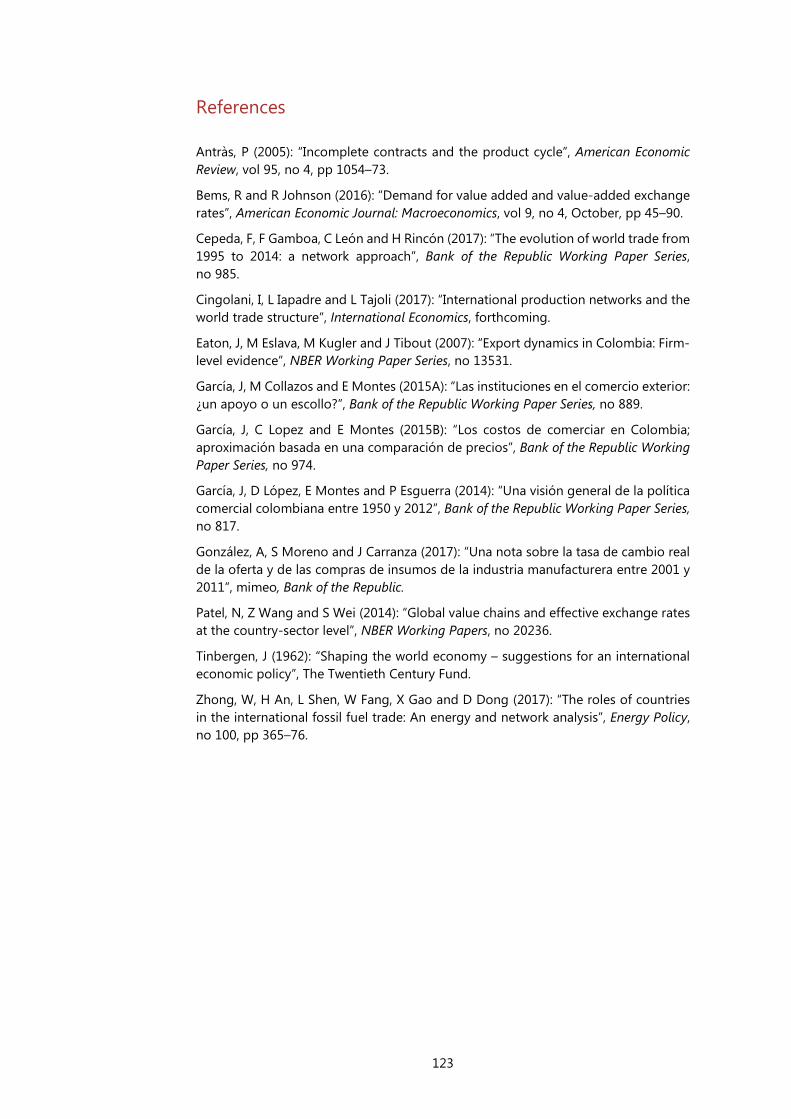
123
References
Antràs, P (2005): “Incomplete contracts and the product cycle”, American Economic Review, vol 95, no 4, pp 1054–73.
Bems, R and R Johnson (2016): “Demand for value added and value-added exchange rates”, American Economic Journal: Macroeconomics, vol 9, no 4, October, pp 45–90.
Cepeda, F, F Gamboa, C León and H Rincón (2017): “The evolution of world trade from 1995 to 2014: a network approach”, Bank of the Republic Working Paper Series, no 985.
Cingolani, I, L Iapadre and L Tajoli (2017): “International production networks and the world trade structure”, International Economics, forthcoming.
Eaton, J, M Eslava, M Kugler and J Tibout (2007): “Export dynamics in Colombia: Firm-level evidence”, NBER Working Paper Series, no 13531.
García, J, M Collazos and E Montes (2015A): “Las instituciones en el comercio exterior: ¿un apoyo o un escollo?”, Bank of the Republic Working Paper Series, no 889.
García, J, C Lopez and E Montes (2015B): “Los costos de comerciar en Colombia; aproximación basada en una comparación de precios”, Bank of the Republic Working Paper Series, no 974.
García, J, D López, E Montes and P Esguerra (2014): “Una visión general de la política comercial colombiana entre 1950 y 2012”, Bank of the Republic Working Paper Series, no 817.
González, A, S Moreno and J Carranza (2017): “Una nota sobre la tasa de cambio real de la oferta y de las compras de insumos de la industria manufacturera entre 2001 y 2011”, mimeo, Bank of the Republic.
Patel, N, Z Wang and S Wei (2014): “Global value chains and effective exchange rates at the country-sector level”, NBER Working Papers, no 20236.
Tinbergen, J (1962): “Shaping the world economy – suggestions for an international economic policy”, The Twentieth Century Fund.
Zhong, W, H An, L Shen, W Fang, X Gao and D Dong (2017): “The roles of countries in the international fossil fuel trade: An energy and network analysis”, Energy Policy, no 100, pp 365–76.

124 BIS Papers No 100

BIS Papers No 100 125
Foreign capital and domestic productivity in the Czech Republic*
Mojmír Hampl and Tomáš Havránek1
Abstract
In this paper we take stock of the evidence concerning the effect of foreign direct investment (FDI) on the productivity of locally owned firms in the Czech Republic. To this end, we collect 332 estimates previously reported in journal articles, working papers and PhD theses. We find that the mean reported externality arising for domestic firms due to the presence of foreign firms (the “FDI spillover”) is zero. There is no evidence of publication bias, ie no sign of selective reporting of results that are statistically significant and show an intuitive sign. Nevertheless, we find that the overall spillover effect is positive and large when more weight is placed on estimates that conform to best-practice methodology. Our results suggest that, as of 2018, a 10-percentage-point increase in foreign presence is likely to lift the productivity of domestic firms by 11%. The effect is even larger for joint ventures, reaching 19%.
Keywords: foreign direct investment, productivity, spillovers, meta-analysis.
JEL classification: C83, F23, 012.
1 Czech National Bank

126 BIS Papers No 100
Introduction
Many governments, especially those in emerging and transition countries, have sought to attract foreign direct investment. Foreign capital should help lift productivity in the host country in two general ways: directly (by increasing the productivity of acquired firms) and indirectly (by diffusing technology to local competitors, suppliers and buyers). The direct effect does not constitute an externality, because foreign investors receive the profits generated by the now-more-efficient acquired company. For this reason, it cannot form a rationale for providing subsidies to foreign investors. The indirect channel of productivity enhancement, in contrast, has been frequently used in the policy debate on subsidies. Therefore, in this paper we concentrate on the indirect channel (typically called “FDI productivity spillovers” in the literature) and refer readers interested in the direct channel to the comprehensive survey by Hanousek et al (2011).
FDI spillovers can arise in three scenarios. First, the local competitors of foreign firms can imitate foreign technology (horizontal spillovers). Second, local suppliers can benefit from increased pressure to raise quality and sometimes from direct inspections and quality control commissioned by foreign firms (backward spillovers). Third, local buyers of intermediate products sold by foreign firms can benefit from the increased quality of those products (forward spillovers). Both suppliers and buyers can, of course, also imitate the technology used by foreigners, although this channel is more straightforward for firms that are present in the same industry as foreign firms. More details on technology transfer related to FDI are available in a series of surveys by Havránek and Iršová (2011, 2012) and Iršová and Havránek (2013).
In this paper, we provide the first systematic and quantitative synthesis of the evidence on FDI spillovers in the Czech Republic.2 We inspect the literature and find 332 estimates of horizontal, backward and forward spillovers previously reported in various articles, papers and reports. For each estimate, we collect variables that reflect the context in which the estimate is obtained (such as data characteristics, estimation methods, control variables and additional aspects related to quality). Next, we investigate how the reported results are influenced by those variables. We also investigate publication bias, that is, the effect of statistical significance and the obtained sign on the probability of reporting.
Our results suggest that the mean estimates of horizontal, backward and forward spillovers are similar and close to zero when all estimates are given the same weight. We find no evidence of publication bias: all results, positive and negative, significant and insignificant, seem to have a similar probability of being reported. Nevertheless, we document that the reported results depend systematically on study design. Data and methodology matter for the published estimates of spillovers. In particular, the spillover estimates are substantially larger for more recent data and when researchers have access to detailed information on firm-to-firm linkages. Joint ventures of foreign and domestic firms are especially beneficial for the productivity of domestic companies: as of 2018, a 10-percentage-
2 Examples of well written previous meta-analyses relevant to comparative economics include
Fidrmuc and Korhonen (2006), Cuaresma et al (2014), Iwasaki and Tokunaga (2016), and Iwasaki and Kočenda (2017).
BIS Papers No 100 127
point increase in the incidence of joint ventures is expected to raise domestic productivity by 19%.
Data
Several studies have been conducted on FDI spillovers in the Czech Republic, and we use the results of these studies as our data. In this way we can provide robust conclusions and fully exploit the work of previous researchers. Unfortunately, not all the studies in the literature can be used for this purpose. We can only collect estimates that are quantitatively comparable, ie that answer the following question: what is the percentage increase in the productivity of domestic firms when the foreign presence in connected firms increases by 1 percentage point? Additionally, we require that the studies also report backward or forward spillovers, not only horizontal ones (to avoid the obvious omitted variable problem). Almost all studies do indeed include backward or forward spillovers. Nevertheless, several good recent studies cannot be used for other reasons: Pavlínek and Žížalová (2016) report survey results and not numerical values on FDI spillovers, while Kosová (2010) and Ayyagari and Kosová (2010) focus on domestic firm entry and crowding out induced by foreign direct investment.
We searched the Google Scholar, EconLit, and Scopus databases for potentially useful studies on FDI spillovers in the Czech Republic. After employing the aforementioned inclusion criteria, we are left with eight studies (shown in Graph 1), which nevertheless provide a wealth of data: 332 estimates of FDI spillovers under various settings. The studies were published between 2003 and 2013 and, taken together, cover tens of thousands of firms in almost all industries and service sectors of the Czech economy. Graph 1 demonstrates that the results of these studies vary widely. Differences are apparent not only across studies, but also within individual studies: every single study reports both positive and negative results, making immediate inference hard.
The summary statistics of our data set for horizontal, backward and forward spillovers are very similar.3 For all three categories we obtain a negative mean estimate: –0.1 in the case of horizontal spillovers, –0.16 in the case of backward spillovers, and –0.09 in the case of forward spillovers. For this reason, in the remainder of the paper we will analyse these spillover categories jointly. Interestingly, the median reported estimates are always larger than the mean ones, which might suggest publication bias (in particular, preferential selection of negative results). The median is –0.06 for horizontal spillovers, 0.11 for backward spillovers, and 0.01 for forward spillovers. We turn to the problem of publication bias in the next section.
3 In all computations, we winsorise the estimates at the 5% level because of several outliers in the
data (inherent in any meta-analysis). The winsorisation does not affect our main results.

128 BIS Papers No 100
Estimates of FDI spillovers vary both across and within studies Graph 1
Publication bias
Publication bias arises when authors, editors or referees prefer estimates that are statistically significant or display the sign dictated by the theory. For example, it has been shown repeatedly that researchers in economics tend to avoid reporting positive estimates of price elasticities. Very few researchers believe that gasoline, for example, could be a Giffen good, but they will sometimes obtain positive elasticity estimates due to noise in the data and imprecision in methodology (see, for example, Havránek et al (2012) and Havránek et al (2017)). When some estimates are selectively omitted from the literature, the mean reported estimates get biased, typically away from zero. Publication bias has been acknowledged as one of the most serious problems of current economics research, because it directly affects takeaways from the literature and thus significantly hampers efforts to pursue evidence-based policy (Ioannidis et al (2017)).
In the literature on FDI spillovers, one might expect to see some selective reporting against negative and insignificant estimates. As discussed in the introduction, there are many reasons why researchers should expect to obtain positive spillover estimates; moreover, statistical significance makes it easier to “sell” the results. But the theory is consistent with negative spillovers as well. The case is most salient for horizontal spillovers, where the entry of foreign firms immediately increases competition for domestic firms currently present in the industry. This competition hampers their returns to scale and may therefore reduce productivity.
-6 -4 -2 0 2 4Estimate of the spillover effect
Vacek (2010)
Vacek (2007)
Stančík (2009)
Stančík (2007)
Geršl et al. (2007)
Geršl (2008)
Damijan et al. (2013)
Damijan et al. (2003)

BIS Papers No 100 129
Similarly, in relation to backward spillovers, foreign firms may choose to import intermediate goods instead of purchasing them from local companies. Foreign firms may also produce intermediate goods primarily for export, thereby reducing the extent of forward spillovers.
The tool used most commonly to examine publication bias is the funnel plot. It is a scatter plot of the estimates, shown on the horizontal axis, and the precision of those estimates, shown on the vertical axis. In theory, the most precise estimates should be close to the mean underlying effect, while less precise estimates should be more dispersed. Consequently, a symmetrical inverted “funnel” should arise in the scatter plot. The symmetry of the funnel is crucial, because it tells us something about how negative and positive estimates are treated in relation to each other. If more positive than negative estimates with the same level of precision are reported, we suspect publication bias against negative estimates, and vice versa.
The funnel plot for spillover estimates in the Czech Republic is shown in Graph 2. We can see that the funnel is remarkably symmetrical, which is rare in economics: there is no prima facie evidence of publication bias. The most precise spillover estimates are close to zero, indicating that, when no consideration is given to methodology and quality aspects of the individual estimates, there seems to be little relation between foreign presence and local productivity in the Czech Republic. (This is a result that we will challenge later.)
The funnel plot of the spillover estimates suggests no publication bias Graph 2
05
1015
20Pr
ecis
ion
of th
e es
timat
e (1
/SE)
-4 -2 0 2 4Estimated spillover effect

130 BIS Papers No 100
We can also test the symmetry of the funnel plot formally, using the funnel asymmetry test. The test involves regressing the spillover estimates on the standard errors of those estimates. Because the methods used by researchers imply that the ratio of the estimates to their standard errors has a t-distribution, there should be no statistical relation between these two quantities. Indeed, our regressions in Table 1 imply no statistically significant publication bias. First, we apply simple regression (with standard errors clustered at the study level). Second, we add study-level fixed effects. Third, we run weighted least squares with weights proportional to the precision of the individual estimates. All specifications show no evidence of selective reporting and also no evidence of a non-zero mean spillover effect. In the next section we turn to examining the importance of data, methodology and quality aspects.
Funnel asymmetry tests show no publication bias and a zero mean spillover effect Table 1
Ordinary least squares Fixed effects Weighted least squares
Standard error (bias) –0.311 –0.192 –0.436
(0.288) (0.150) (0.367)
Constant (spillover effect) 0.00187 –0.0445 0.0500
(0.175) (0.0581) (0.0721)
Observations 332 332 332
Note: The dependent variable is the spillover estimate. Standard errors, clustered at the study level, are reported in parentheses. The weight in the weighted least squares is the precision of the estimates reported in primary studies.
* p < 0.10, ** p < 0.05, *** p < 0.01
Heterogeneity
So far we have ignored the fact that the studies in our sample differ in more aspects than just precision. These aspects may well affect the reported results, and one may want to place more weight on estimates conducted according to what is considered the best-practice methodology in the literature. All the studies we examine avoid the most common problems in the literature on FDI spillovers, such as using cross-sectional data (and thus not being able to control for unobservable firm-level characteristics) or aggregated data (which gives rise to many problems in addition to the one mentioned in the previous parenthesis). But still, the remaining differences are substantial and we will attempt to control for them.
We will regress the spillover estimates on variables that reflect study design in several ways: choice of data, choice of methodology, and general quality aspects. First, to see whether there are systematic differences in the extent of horizontal, backward, and forward spillovers for the Czech Republic, we include the corresponding dummy variables. We also include a dummy variable that equals one if the study uses a lagged variable for spillovers, that is, if the study assumes that it takes time for spillovers to materialise. Next, we control for the fact that some studies assume a quadratic relation between foreign presence and domestic productivity (but note that we always re-compute the reported coefficients so that

BIS Papers No 100 131
they represent a linear effect evaluated at the sample mean; otherwise the estimates would not be comparable).
Some studies report specifications estimated in differences, and we control for this aspect of study design. We also account for the number of firms used in each study. We include dummy variables that equal one if year fixed effects and sector fixed effects are included in the estimation. The variable Competition reflects whether or not the study controls for industry competition. Some papers study the effect of greenfield investment (or full acquisition of existing plants), while others examine joint ventures; we are also interested in whether spillovers vary for these types of foreign investment. Some estimates are computed for manufacturing and some for service sectors, which we also take into consideration.
An important issue in the literature on FDI spillovers is how to measure the linkages between domestic and foreign firms. Researchers typically compute industry-level measures that use input-output tables and the share of foreign presence in individual industries (in terms of assets or output). Vacek (2010) criticises this approach and collects a unique data set that reflects the real linkages between individual Czech and foreign firms. We will investigate whether this method yields systematically larger spillover estimates. An important issue is the econometric technique used to estimate spillovers; many studies use fixed effects, while several others use the general method of moments (GMM), pooled ordinary least squares, or random effects. We include corresponding dummy variables for these choices of methodology. Finally, to reflect quality aspects potentially not captured by all the data and method variables above, we include the recursive RePEc impact factor of the outlet in which the study was published and also the number of citations in Google Scholar that the paper receives per year.
The results of regressing the spillover estimates on all the variables introduced in this section are shown in Table 2. The table presents two models (note that in all models we cluster the standard errors at the level of individual studies, because we suspect that estimates reported within individual studies are not independent). In the first model, we simply add all the variables and estimate one regression. Next, we follow the common general-to-specific approach and exclude the variables that are jointly insignificant at the 5% level. We are left with the specific model in the right-hand part of the table. Our results suggest that about half of the variables are important for explaining why the spillover estimates vary so much.
We find that, ceteris paribus, studies assuming a quadratic relationship between foreign presence and domestic productivity tend to find larger spillovers. An important finding is that spillovers increase with the year of the data: newer data sets are associated with larger spillovers. The inclusion of year fixed effects and controlling for industry competition reduce the reported spillover estimates in individual studies. Joint ventures of foreign and domestic companies generate much larger positive spillovers than companies fully owned by foreign investors. It also matters how the linkages are computed: when real individual linkages are available, the reported spillovers are substantially larger than when industry-level constructs are used. Different econometric techniques yield statistically significantly different results, but the difference of about 0.1 is small in economic terms. Study citations and the impact factor of the outlet are not important for the reported spillover effects.

132 BIS Papers No 100
Factors influencing the reported spillover estimates Table 2
General model Specific model
Forward 0.0773 (0.401)
Horizontal 0.286 (0.311)
Lagged –0.0534 (0.0351)
Quadratic 0.390 (0.280) 0.565** (0.183)
Differences 0.0117 (0.0847)
No. of firms 0.0930 (0.0801)
Data year 0.150*** (0.0184) 0.135*** (0.0190)
Year FE –0.278*** (0.0713) –0.333*** (0.0237)
Sector FE 0.0136 (0.0650)
Competition –0.360 (0.363) –0.573*** (0.0530)
Fully owned 0.601 (0.439)
Joint ventures 1.282** (0.439) 0.733*** (0.0364)
Services 0.0143 (0.208)
Assets –0.466** (0.169) –0.463*** (0.0542)
Output –0.162 (0.106) –0.188*** (0.0503)
POLS 0.156* (0.0672) 0.205*** (0.00675)
Random 0.0585 (0.0561) 0.0909*** (0.0258)
GMM –0.0951** (0.0303) –0.0765** (0.0307)
Real linkages 1.097** (0.428) 0.353*** (0.0237)
Impact factor –3.035 (2.975)
Citations 0.0471 (0.0406)
Pub. year –0.127 (0.0840)
Constant –0.704 (0.774) –0.202** (0.0832)
Observations 332 332
Note: The dependent variable is the spillover estimate. Standard errors, clustered at the study level, are reported in parentheses. The specific model is achieved by discarding variables that are jointly insignificant at the 5% level. FE = fixed effects. POLS = pooled ordinary least squares. GMM = general method of moments.
* p < 0.10, ** p < 0.05, *** p < 0.01
We can use the results of the specific model to compute the mean spillover estimate conditional on the best practice applied in the literature. In other words, we use all the estimates, but place more weight on the ones that use the preferred approach. This can be achieved simply by constructing fitted values from the regression and choosing the preferred values of the variables. We prefer linear spillover estimates (preferring the quadratic method would imply even larger effects) and control for year fixed effects and competition measures. For the year of the data, we plug in 2018 in order to estimate current effects – assuming that the trend that we see in the literature has continued to this day. We prefer data on real linkages and the GMM technique.
The resulting spillover estimate is 1.1 on average and 1.9 when we consider only joint ventures. Both these estimates are statistically significant at the 1% level. In economic terms, the effect is large: a more than one-to-one relation between

BIS Papers No 100 133
foreign presence and domestic productivity. Few countries have been found in the literature to show such strong FDI spillovers.
Bayesian model averaging
In this section we present a robustness check that takes into account the model uncertainty inherent in meta-analysis. We are never sure ex ante which of the many potential variables that may explain heterogeneity in the reported estimates should really be included in the best meta-analysis model. In the previous section we chose a simple way of dealing with model uncertainty: we estimated the model that included all the variables and then excluded those that were jointly insignificant at the 5% level. Nevertheless, obviously there are many possible models (with different combinations of all the potential variables) that we did not explore. Such an exploration can be achieved using Bayesian model averaging.
Bayesian model averaging was designed specifically to tackle model uncertainty (Raftery et al (1997)). The essence of the technique is to estimate all the possible models containing different combinations of explanatory variables and then weight them based on how well they fit the data (which is captured by a statistic called the posterior model probability). Because in our case there are too many model combinations, we use the Model Composition Markov Chain Monte Carlo algorithm, which walks through the models with the highest posterior probabilities. To ensure good convergence, we use one million iterations and 500,000 burn-ins. Each variable is then assigned a posterior inclusion probability (PIP), which can be thought of as the Bayesian analogy of statistical significance and is computed as the sum of the posterior model probabilities for the models in which the variable is included.
Model inclusion in Bayesian model averaging Graph 3
The results are shown in Graph 3. Models are sorted from left to right according to posterior model probability (depicted on the horizontal axis). Variables are sorted

134 BIS Papers No 100
from top to bottom according to posterior inclusion probability. In consequence, the best models are shown on the left and the most useful variables at the top of the figure. We can see that the very best model includes only two variables, Joint ventures and Assets, but that this model cannot explain the remaining 89% of the model mass. The other important variables are Horizontal, Real linkages, Quadratic, and Data year, but for all of them the posterior inclusion probabilities fall short of 50%.
Results of Bayesian model averaging Table 3
PIP Post. mean Post. std. dev.
Forward 0.053 0.001 0.024
Horizontal 0.402 0.094 0.133
Lagged 0.065 -0.005 0.032
Quadratic 0.178 0.072 0.191
Differences 0.104 -0.016 0.063
No. of firms 0.089 -0.003 0.021
Data year 0.144 0.011 0.035
Year FE 0.061 -0.010 0.067
Sector FE 0.053 0.004 0.041
Competition 0.081 -0.018 0.100
Fully owned 0.090 0.016 0.068
Joint ventures 1.000 0.785 0.142
Services 0.046 0.000 0.055
Assets 1.000 -0.821 0.147
Output 0.055 -0.004 0.033
POLS 0.051 0.002 0.042
Random 0.061 0.011 0.071
GMM 0.047 -0.001 0.049
Real linkages 0.344 0.109 0.179
Impact factor 0.053 -0.023 0.246
Citations 0.055 0.000 0.003
Pub. year 0.094 0.003 0.015
As with other Bayesian approaches, Bayesian model averaging may be sensitive to the choice of priors. In particular, one has to choose priors for regression parameters4 and model size. In the results reported so far, we have used the unit information prior and uniform model prior, which tend to work well in predictive exercises. Nevertheless, other researchers might prefer different priors. As another
4 We follow the common approach and choose the conservative prior of zero for each parameter.
Note that this practice generally drives the posterior means for coefficients in Bayesian model averaging towards zero, which helps explain why almost all the estimates are now smaller in absolute value than what we saw previously with OLS. For all the variables previously identified by our specific model, however, the estimated sign remains the same.
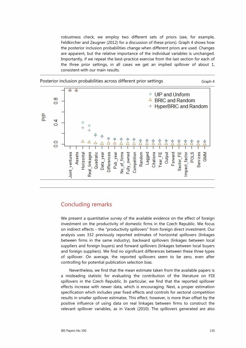
BIS Papers No 100 135
robustness check, we employ two different sets of priors (see, for example, Feldkircher and Zeugner (2012) for a discussion of these priors). Graph 4 shows how the posterior inclusion probabilities change when different priors are used. Changes are apparent, but the relative importance of the individual variables is unchanged. Importantly, if we repeat the best-practice exercise from the last section for each of the three prior settings, in all cases we get an implied spillover of about 1, consistent with our main results.
Posterior inclusion probabilities across different prior settings Graph 4
Concluding remarks
We present a quantitative survey of the available evidence on the effect of foreign investment on the productivity of domestic firms in the Czech Republic. We focus on indirect effects – the “productivity spillovers” from foreign direct investment. Our analysis uses 332 previously reported estimates of horizontal spillovers (linkages between firms in the same industry), backward spillovers (linkages between local suppliers and foreign buyers) and forward spillovers (linkages between local buyers and foreign suppliers). We find no significant differences between these three types of spillover. On average, the reported spillovers seem to be zero, even after controlling for potential publication selection bias.
Nevertheless, we find that the mean estimate taken from the available papers is a misleading statistic for evaluating the contribution of the literature on FDI spillovers in the Czech Republic. In particular, we find that the reported spillover effects increase with newer data, which is encouraging. Next, a proper estimation specification which includes year fixed effects and controls for sectoral competition results in smaller spillover estimates. This effect, however, is more than offset by the positive influence of using data on real linkages between firms to construct the relevant spillover variables, as in Vacek (2010). The spillovers generated are also

136 BIS Papers No 100
much larger for joint ventures of foreign and local firms than for fully foreign-owned firms.
Using these findings, we compute the spillover value implied by the best practice in the literature for the year 2018. The result is 1.1 overall, implying that a 10-percentage-point increase in foreign presence increases domestic productivity by 11%. This is a large figure compared to studies on FDI spillovers in other countries; without doubt, the effect is economically significant. Moreover, the positive effect reaches 19% when joint ventures are considered. All in all, we conclude that, based on the available empirical evidence, foreign direct investment has been beneficial to the productivity of locally owned firms in the Czech Republic.
References
Ayyagari, M and R Kosová (2010): “Does FDI facilitate domestic entry? Evidence from the Czech Republic”, Review of International Economics, vol 18, no 1, pp 14–29.
Cuaresma, J, J Fidrmuc and M Hake (2014): “Demand and supply drivers of foreign currency loans in CEECs: A meta-analysis”, Economic Systems, vol 38, no 1, pp 26–42.
Damijan, J, M Knell, B Majcen and M Rojec (2003): “Technology transfer through FDI in top-10 transition countries: how important are direct effects, horizontal and vertical spillovers?”, William Davidson Institute Working Papers Series, no 549, William Davidson Institute at the University of Michigan.
Damijan, J, M Rojec, B Majcen and M Knell (2013): “Impact of firm heterogeneity on direct and spillover effects of FDI: Micro-evidence from ten transition countries”, Journal of Comparative Economics, vol 41, no 3, pp 895–922.
Feldkircher, M and S Zeugner (2012): “The impact of data revisions on the robustness of growth determinants – a note on determinants of economic growth: will data tell?”, Journal of Applied Econometrics, vol 27, no 4, pp 686–94.
Fidrmuc, J and I Korhonen (2006): “Meta-analysis of the business cycle correlation between the euro area and the CEECs”, Journal of Comparative Economics, vol 34, no 3, pp 518–37.
Geršl, A (2008): “Productivity, export performance, and financing of the Czech corporate sector: the effects of foreign direct investment”, Czech Journal of Economics and Finance, vol 58, pp 232–47.
Geršl, A, I Rubene, and T Zumer (2007): “Foreign direct investment and productivity spillovers: updated evidence from central and eastern Europe”, CNB Working Papers, no 2007/8, Czech National Bank, Research Department.
Hanousek, J, E Kočenda and M Maurel (2011): “Direct and indirect effects of FDI in emerging European markets: a survey and meta-analysis”, Economic Systems, vol 35, no 3, pp 301–22.
Havránek, T and Z Iršová (2011): “Estimating vertical spillovers from FDI: why results vary and what the true effect is”, Journal of International Economics, vol 85, no 2, pp 234–44.

BIS Papers No 100 137
——— (2012): “Survey article: publication bias in the literature on foreign direct investment spillovers”, Journal of Development Studies, vol 48, no 10, pp 1375–96.
Havránek, T, Z Iršová and K Janda (2012): “Demand for gasoline is more price-inelastic than commonly thought”, Energy Economics, vol 34, no 1, pp 201–7.
Havránek, T, Z Iršová and O Zeynalova (2017): “Tuition fees and university enrollment: a meta-analysis”, Institute of Economic Studies Working Papers, no 2017/16, Charles University Prague, Faculty of Social Sciences.
Ioannidis, J, C Doucouliagos and T Stanley (2017): “The power of bias in economics research”, Economic Journal, vol 127, F236–F265.
Iršová, Z and T Havránek (2013): “Determinants of horizontal spillovers from FDI: evidence from a large meta-analysis”, World Development, vol 42, issue C, pp 1–15.
Iwasaki, I and M Tokunaga (2016): “Technology transfer and spillovers from FDI in transition economies: a meta-analysis”, Journal of Comparative Economics, vol 44, no 4, pp 1086–114.
Iwasaki, I and E Kočenda (2017): “Are some owners better than others in Czech privatized firms? Even meta-analysis can’t make us perfectly sure”, Economic Systems, vol 41, no 4, pp 537–68.
Kosová, R (2010): “Do foreign firms crowd out domestic firms? Evidence from the Czech Republic”, Review of Economics and Statistics, vol 92, no 4, pp 861–81.
Pavlínek, P and P Žížalová (2016): “Linkages and spillovers in global production networks: firm-level analysis of the Czech automotive industry”, Journal of Economic Geography, vol 16, no 2, pp 331–63.
Raftery, A, D Madigan, and J Hoeting (1997): “Bayesian model averaging for linear regression models”, Journal of the American Statistical Association, vol 92, pp 179–91.
Stančík, J (2007): “Horizontal and vertical FDI spillovers: recent evidence from the Czech Republic”, CERGE-EI Working Papers, no 340, Center for Economic Research and Graduate Education – Economics Institute, Prague.
——— (2009): “FDI spillovers in the Czech Republic: takeovers vs. greenfields”, European Economy – Economic Papers 2008–2015, no 369, Directorate General Economic and Financial Affairs (DG ECFIN), European Commission.
Vacek, P (2007): “Productivity spillovers from foreign direct investment: industry-level analysis”, in Essays on International Productivity Spillovers, PhD thesis, Cornell University.
——— (2010): “Productivity gains from exporting: do export destinations matter?”, Institute of Economic Studies Working Papers, no 2010/18, Charles University Prague, Faculty of Social Sciences.

138 BIS Papers No 100

BIS Papers No 100 139
Assessing the impact of globalisation: Lessons from Hong Kong
Lillian Cheung, Eric Wong, Philip Ng and Ken Wong*
Abstract
Driven largely by unique economic and political factors, Hong Kong SAR was a globalised economy long before the advent of global value chains in the 1990s. In particular, Hong Kong’s role as a link between Mainland China and the rest of the world strengthened over time, as did its status as an international financial centre. The effects of globalisation on Hong Kong are multi-faceted, ranging from higher potential vulnerability to external macro-financial shocks and structural adjustments in the labour market, and to widening income and wealth inequality. The experience of Hong Kong suggests that a sound monetary regime, high flexibility in the labour market and a robust framework for financial supervision can help alleviate the costs and risks associated with globalisation. We conclude by highlighting some future challenges facing the Hong Kong economy amid globalisation.
Keywords: globalisation, international, Hong Kong.
JEL classification: F40, F6, N1, N3.
* Research Department, Hong Kong Monetary Authority. Any further correspondence should bedirected to Eric Wong, email: [email protected]. The views expressed here belong to the authors alone and do not necessarily represent those of the Hong Kong Monetary Authority.

140 BIS Papers No 100
1. Background
Hong Kong SAR was a globalised economy long before the advent of global value chains in the 1990s. As indicated by trade and financial openness, two key dimensions of the degree of globalisation for an economy, Hong Kong has considerably exceeded the world averages since data were available (Graphs 1 and 2). Indeed, Hong Kong may have become integrated into the global economy as early as the 1960s.
The globalisation of Hong Kong is driven largely by unique economic and political conditions. Given its small domestic market and lack of natural resources, it was natural for Hong Kong to evolve into a flexible, adaptive and outward-looking economy in order to maintain its competitiveness. The tendency towards an open economy was reinforced by developments in Mainland China. In particular, before Mainland China opened up in the late 1970s, Hong Kong’s political isolation from its motherland and a series of events in Mainland China, including the civil war in the 1940s and the Cold War trade embargos in the late 1940s and 1950s, helped to develop Hong Kong as a unique link between Mainland China and the rest of the world. After Mainland China opened up, Hong Kong’s role was further consolidated on the back of Mainland China’s economic reforms and financial liberalisation. Leveraging on the key intermediary role between Mainland China and the rest of the world, Hong Kong has become a highly globalised economy.
Although it is difficult to generalise, Hong Kong’s case could shed light on what challenges an economy may face amid globalisation and what the policy implications are. The rest of the note is organised as follows. Section 2 provides a brief account of the economic transformation in Hong Kong amid globalisation. Section 3 analyses the macroeconomic and distributional effects of globalisation on Hong Kong and the relevant policy implications. Section 4 concludes by discussing the challenges ahead.
Graph 1: Trade openness: exports and imports of goods and services
Graph 2: Financial openness: external financial assets and liabilities
Sources: C&SD; World Bank. Sources: Lane and Milesi-Ferretti (2017), BIS.
0
50
100
150
200
250
300
350
400
450
500
1961 1971 1981 1991 2001 2011
% of GDP
Hong Kong
World
0
500
1,000
1,500
2,000
2,500
3,000
1961 1971 1981 1991 2001 2011
% of GDP
Hong Kong
World

BIS Papers No 100 141
2. Hong Kong’s economic transformation amid globalisation
As an economy becomes more deeply integrated into the global economy, a rapid transformation may ensue as the economy’s comparative advantages evolve over time due to changes in the external environment. Hong Kong is no exception, and this section therefore attempts to broaden our understanding of globalisation through the lens of Hong Kong’s economic transformation.
Hong Kong as an industrial economy (before the 1980s)
In the late 1940s and 1950s, Hong Kong began to change from an entrepot to an industrial economy. Massive flows of refugees and entrepreneurs fleeing the civil war in Mainland China brought cheap labour, massive capital and technological know-how into Hong Kong. These led Hong Kong to develop as an industrial economy in the 1950s and 1960s specialising in labour-intensive manufacturing industries including clothing, electronics, plastics and toys. Consequently, the share of the secondary sector in GDP increased from about 20% in the early 1950s to around 40% in the 1960s and 1970s (Graph 3). At that time, exports also increased significantly (often at double-digit rates) along with rising trade openness to 150–180% of GDP (Graph 1).
Graph 3: Hong Kong’s economic transformation Graph 4: Import and export trade and
financial services sectors in Hong Kong
Source: C&SD and World Bank Source: C&SD.
Hong Kong as a service-based economy and an international trade and financial centre since the 1980s
With the opening up of the Mainland economy in the late 1970s and rising local labour costs in Hong Kong, Hong Kong firms began to move their labour-intensive production activities to the southern part of Mainland China to take advantage of low labour costs there. The share of manufacturing in Hong Kong’s GDP has declined visibly ever since (Graph 3). However, the relocation of production activities actually increased Hong Kong’s trade openness, as the drop in domestic exports was more than offset by rising trade flows from re-exports and outward processing trades between Hong Kong, Mainland China and the rest of the world. The rising GDP contribution of the import and export trade sector (Graph 4) helped drive the transformation of Hong Kong into a service-based economy. Meanwhile, along with Hong Kong’s growing investments in Mainland China and later massive foreign investment inflows into the Mainland via Hong Kong, Hong Kong also witnessed
0
10
20
30
40
50
60
70
80
90
100
1950 1960 1970 1980 1990 2000 2010
% of GDP
Tertiary sector
Secondary sector
Primary sector
0
5
10
15
20
25
30
35
40
45
1980 1985 1990 1995 2000 2005 2010 2015
Import and export trade
Financial services(including insurance)
% of GDP

142 BIS Papers No 100
rising financial openness as indicated by sharp rises in external financial assets and liabilities to over 1,000% of GDP (Graph 2).
Hong Kong’s role as a link between Mainland China and the rest of the world and its status as an international financial centre were further consolidated after Hong Kong’s reversion to Mainland China in 1997. Further trade liberalisation in Mainland China, especially its accession to the World Trade Organisation in 2001, increased Hong Kong’s total trade flows markedly. Meanwhile, Hong Kong became an international capital hub for Mainland corporates and international investors, which further boosted the domestic financial sector’s contribution to GDP. More recently, with Mainland China entering into a new growth phase and accumulating surplus capital, Hong Kong’s financial sector has played a role in diversifying investment channels for Mainland and international investors. Hong Kong has also facilitated financial liberalisation in Mainland China, serving as the launch pad for many new measures (eg the offshore renminbi business centre, as well as the Stock Connect and Bond Connect Schemes).
3. Macro and distributional effects of globalisation and policy implications
Globalisation has had a far-reaching effect on the Hong Kong economy, as summarised by the following four points.
Strong influence of external factors on Hong Kong’s business cycle fluctuations
Being a highly globalised economy, Hong Kong’s economic performance and its volatility are driven primarily by external factors. Our previous study (HKMA (2014)) shows that external shocks from the United States and Mainland China together could explain more than 70% of cyclical output fluctuations both before and after Hong Kong’s reversion to Mainland China (Table 1).
Table 1: Contribution to cyclical output fluctuations in Hong Kong
Graph 6: Volatility of key macroeconomic variables in Hong Kong
(% share) Contribution from
US China HK
1985Q1-1997Q2 57.1 13.7 29.2
2003Q4-2013Q2 47.6 28.7 23.7
Standard deviation of year-on-year growth
Real GDP Export Import Inflation*
1974Q4-1983Q3 5.8 10.7 13.0 5.1
1984Q1-2017Q3 4.4 9.1 9.6 4.2
Source: HKMA staff estimates.
Note: Variance decomposition over a 20-quarter horizon.
*The series of inflation starts from 1975Q2
Sources: C&SD, HKMA staff estimates.
Policies to dampen economic volatility therefore become crucial in macroeconomic management. In this regard, monetary policy regimes play a particularly important role. Being a small and open economy with a high degree of cyclical synchronisation with the US economy, Hong Kong adopted the Link

BIS Papers No 100 143
Exchange Rate System (LERS, ie pegging the Hong Kong dollar to the US dollar). Empirical studies by Kwan and Liu (1999) and Crosby (2000) found that the LERS reduces the volatility of Hong Kong’s economic performance. Consistent with their findings, the volatility of key macroeconomic variables in Hong Kong is found to have been lower after the implementation of the LERS (Table 2).
Rapid structural changes in the sectoral composition of labour market
As shown in Section 2, globalisation accelerates or even induces economic transformation, causing marked structural changes in the sectoral composition of the labour market. In Hong Kong’s case, employment in the manufacturing sector declined significantly as Hong Kong changed into a service-based economy (Graph 5). Nevertheless, this transformation did not create massive structural unemployment in Hong Kong. Indeed, when the manufacturing sector shrank in Hong Kong, the rise of service sectors, including the trading and logistic sectors, helped to absorb most of the surplus of manufacturing workers. The overall unemployment rate even declined to around 2% in the early 1990s from about 4% in the early 1980s.
Graph 5: Employment by economic sector Graph 6: Change in wages and employment
in five industries, 1994–2004
Source: C&SD. Source: C&SD.
Hong Kong’s smooth economic transformation amid globalisation was
largely underpinned by the flexibility of its labour market. This is reflected in the high responsiveness of wages and employment adjustments among sectors subject to the economic transformation (Graph 6). In particular, when the manufacturing sector lost its competitiveness, its wages growth was below that of other service sectors. By contrast, wage growth in the financial industry outpaced that of other sectors as Hong Kong’s international financial centre expanded. These observations suggest that wage adjustments in Hong Kong faced no major rigidities during the economic transformation and that labour remained highly mobile across sectors.
Government measures also helped smooth economic transformation in Hong Kong. These include increases in investment in education, the establishment of the Employees Retraining Board and the Continuing Education Fund. These measures not only enhanced labour mobility among sectors, but also helped upgrade labour force skills.
0
20
40
60
80
100
120
140
1,500
1,800
2,100
2,400
2,700
3,000
3,300
3,600
94 96 98 00 02 04 06 08 10 12 14 16 18
Financial & business (lhs)Other services (lhs)Manufacturing (rhs)
Person ('000) Person ('000)
-80
-60
-40
-20
0
20
40
60
20 22 24 26 28 30
% c
hang
e in
the
no. o
f wor
kers
% change in wages
Manufacturing
Transportation
Personal services
FinancingTrade and tourism

144 BIS Papers No 100
Increased financial integration with higher international spillover of risks
Globalisation has led to greater financial integration internationally. Of the 195 banks operating in Hong Kong at end-2016, 186 were foreign-owned banks. Indeed, most global systemically important banks have an operation in Hong Kong. This, together with the large banking sector compared with the size of Hong Kong’s economy (ie banking assets/annual GDP in Hong Kong was around 840% at September 2017), means that the Hong Kong economy is potentially more vulnerable to external financial shocks.
Nevertheless, effective banking supervision and the sound fundamentals of banks in Hong Kong have helped to contain the risks associated with external financial shocks. In fact, thanks to its strong capital and liquidity position (Graphs 7 and 8), the banking sector emerged from the Asian financial crisis and Great Financial Crisis (GFC) largely unscathed.
Graph 7: Capitalisation of locally incorporated banks
Graph 8: Liquidity Coverage Ratio
Note: Average consolidated ratio for all authorised institutions to carry on the business of taking deposit.
Source: HKMA.
Note: Average consolidated ratio for all banks in Hong Kong subject to the LCR requirements (i.e. Category 1 institutions in Hong Kong)
Source: HKMA.
Nevertheless, macroprudential measures have been deployed extensively by
the Hong Kong Monetary Authority (HKMA) to reduce the risks of financial instability after the global financial crisis. In particular, in view of rising property prices in Hong Kong amid strong capital inflows and the zero interest rate environment after the GFC, the HKMA has implemented eight rounds of prudential measures since late 2009 to help banks strengthen risk management in their mortgage loan businesses.
Widening income and wealth inequalities
Hong Kong saw widening income inequality amid globalisation. Income inequality measured by the Gini coefficient rose quickly from 0.43 in 1971 to 0.53 in 2001 (Graph 9) mainly as a result of immigration and economic transformation, two often citied causes of rising income inequality amid globalisation. Specifically, massive inflows of immigrants from Mainland China before the 1980s increased the number of low-income households as their education and skill levels were relatively
8
10
12
14
16
18
20%
Tier-one capital adequacy ratioCapital adequacy ratio
2007 2008 2009 2010 2011 2012 2013 2014 2015 2016 2017
Introduction of Basel III
020406080
100120140160180
2015
Q1
2015
Q2
2015
Q3
2015
Q4
2016
Q1
2016
Q2
2016
Q3
2016
Q4
2017
Q1
2017
Q2
2017
Q3
2017
Q4
LCR Statutory minimum requirement of LCR
%
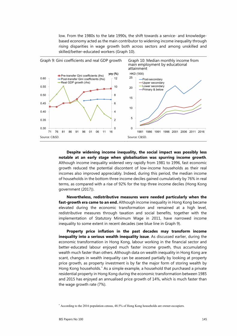
BIS Papers No 100 145
low. From the 1980s to the late 1990s, the shift towards a service- and knowledge-based economy acted as the main contributor to widening income inequality through rising disparities in wage growth both across sectors and among unskilled and skilled/better-educated workers (Graph 10).
Graph 9: Gini coefficients and real GDP growth Graph 10: Median monthly income from
main employment by educational attainment
Source: C&SD. Source: C&SD.
Despite widening income inequality, the social impact was possibly less notable at an early stage when globalisation was spurring income growth. Although income inequality widened very rapidly from 1981 to 1996, fast economic growth reduced the potential discontent of low-income households as their real incomes also improved appreciably. Indeed, during this period, the median income of households in the bottom three income deciles gained cumulatively by 76% in real terms, as compared with a rise of 92% for the top three income deciles (Hong Kong government (2017)).
Nevertheless, redistributive measures were needed particularly when the fast-growth era came to an end. Although income inequality in Hong Kong became elevated during the economic transformation and remained at a high level, redistributive measures through taxation and social benefits, together with the implementation of Statutory Minimum Wage in 2011, have narrowed income inequality to some extent in recent decades (see blue line in Graph 9).
Property price inflation in the past decades may transform income inequality into a serious wealth inequality issue. As discussed earlier, during the economic transformation in Hong Kong, labour working in the financial sector and better-educated labour enjoyed much faster income growth, thus accumulating wealth much faster than others. Although data on wealth inequality in Hong Kong are scant, changes in wealth inequality can be assessed partially by looking at property price growth, as property investment is by far the major form of storing wealth by Hong Kong households.* As a simple example, a household that purchased a private residential property in Hong Kong during the economic transformation between 1985 and 2015 has enjoyed an annualised price growth of 14%, which is much faster than the wage growth rate (7%).
* According to the 2016 population census, 48.5% of Hong Kong households are owner-occupiers.
0
2
4
6
8
10
12
0.30
0.35
0.40
0.45
0.50
0.55
0.60
71 76 81 86 91 96 01 06 11 16
Pre-transfer Gini coefficients (lhs)Post-transfer Gini coefficients (lhs)Real GDP growth (rhs)
yoy (%)yoy (%)
0
5
10
15
20
25
1981 1986 1991 1996 2001 2006 2011 2016
Post-secondaryUpper secondaryLower secondaryPrimary & below
HKD ('000)

146 BIS Papers No 100
Nevertheless, housing policies in Hong Kong have helped alleviate the widening wealth inequality to some extent. The government has launched the home ownership scheme (HOS) in 1978 by which households who cannot afford private housing can purchase a government-subsidised apartment with a price much lower than market prices. Such HOS and other similar government programmes have so far helped a large number of households to get onto the housing ladder. The latest statistics show that there are nearly 400,000 government-subsidised housing units, which account for about 15% of the total housing stock in Hong Kong.
4. Conclusion
Three potential challenges face the Hong Kong economy amid globalisation. First, in view of the higher potential vulnerability to external financial shocks, central banks may need to play an even more active role in mitigating the associated risks, as the potential impacts of such shocks on the economy could be much larger than before.
Secondly, Hong Kong’s case demonstrates that globalisation can cause rapid structural changes in the labour market. While Hong Kong’s flexible labour market has so far helped to smooth the path of economic transformation, labour market adjustments will be more difficult when Hong Kong enters into the next stage of economic transformation in view of the higher degree of financial market expertise required and greater international competition in labour markets.
Finally, distributional effects remain a big challenge, particularly widening wealth inequality. Importantly, the unconventional post-crisis monetary policies adopted by major advanced economies may have a significant impact on wealth inequality through effects on asset price inflation, which could amplify the discontents of globalisation (See Chan (2017)).

BIS Papers No 100 147
References
Chan, N (2017): “Norman Chan on globalisation, technological innovation, monetary policy, and the distribution of income and wealth”, HKMA inSight articles, 6 September.
Crosby, M (2000): “Exchange rate volatility and macroeconomic performance in Hong Kong”, HKIMR Working Papers, no 03/2000.
Kwan, Y and F Liu (1999): “How well has the currency board performed? Evidence from Hong Kong”, mimeo, Hong Kong University of Science and Technology.
Lane, P and G Milesi-Ferretti (2017): “International financial integration in the aftermath of the global financial crisis”, IMF Working Papers, WP/17/115.
Hong Kong Monetary Authority (2014): “Box 3: Hong Kong’s economic trend and cycle synchronisation with Mainland China and the US”, Half-yearly Monetary and Financial Stability Report, September 2014.
Hong Kong Government (2017): “Box 5.2: The Gini coefficients of Hong Kong in 2016: trends and interpretations”, Half-yearly Economic Report 2017.

148 BIS Papers No 100
BIS Papers No 100 149
The external and domestic drivers of inflation: the case study of Hungary
Erzsébet Éva Nagy and Veronika Tengely1
Abstract
Factors that have tended to result in declining inflation rates worldwide since 2013 include subdued global economic activity, declining energy and commodity prices, technological innovation and inflation expectations that are anchored at historically low levels around the world. The relationship between globalisation and inflation is a popular research topic among economists. According to much of the literature, the influence of globalisation and external factors on national inflation rates has increased in recent years. In this paper we investigate how external and domestic drivers affect inflation in Hungary. The country is an interesting case study, since its openness has grown significantly. Indeed, Hungary is now one of the most open economies in the EU. The Hungarian experience could thus be interesting for countries with an increasing trend towards openness. Using several statistical methods, we examined and analysed the impact of external and domestic drivers of Hungarian inflation, and how these external factors and their effect on inflation have varied in time. Our results show that the role of external factors in domestic inflation developments has strengthened in recent years. Especially after 2012, changes in inflation in Hungary were influenced mainly by external effects.
Keywords: external factors, globalisation, inflation, Phillips curve, principal components, SVAR models.
JEL classification: C53, E31, E37, F02, F41, F62.
1 Erzsébet Éva Nagy ([email protected]) is an Analyst at the Directorate Economic Forecast and Analysis
of the Magyar Nemzeti Bank (The Central Bank of Hungary: MNB). Veronika Tengely ([email protected]) is a Junior Analyst at the Directorate Economic Forecast and Analysis of the MNB. The views expressed are those of the authors and do not necessarily reflect the official view of the MNB.

150 BIS Papers No 100
Introduction
Factors that have favoured declining inflation rates at global level since 2013 include subdued global economic activity, declining energy and commodity prices, technological innovation and inflation expectations anchored at historically low levels around the world. As a result of rising commodity prices at end-2016 and in early 2017, inflation rates have moved away from close-to-zero levels, but are still tending to fall short of central bank targets.
In contrast to global inflation rates, economic performance has varied from region to region after the crisis, which is also corroborated by the significantly different levels of unemployment in the European Union (Graph 1, left-hand panel). After 2012, the standard deviation of unemployment rates increased remarkably. Despite the different phase of the labour market cycle, no divergence could be detected in inflation dynamics; indeed, inflation rates have tended to remain at generally low levels in recent years (Graph 1, right-hand panel). In this regard, the question is what role might global common factors play in these developments.
The most common reasons for the growing correlation between inflation rates are globalisation and integration into global production processes (the role of global value chains), which may have amplified the impact of international business cycles on inflation. The effect of globalisation is felt through various channels. Increased trade openness, higher competition as a result of economic integration, the global division of labour and the appearance of new
Standard deviations of unemployment rates and inflation rates in the EU Graph 1
Sources: Eurostat, MNB.
0.00.51.01.52.02.53.03.54.04.55.0
2004–12 2013–17 2004–12 2013–17
Unemployment rate Inflation rate
2004–12 2013–17
Percentage point
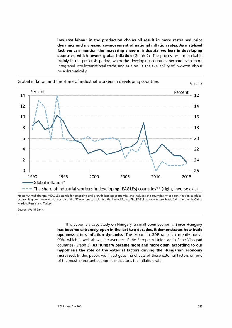
BIS Papers No 100 151
low-cost labour in the production chains all result in more restrained price dynamics and increased co-movement of national inflation rates. As a stylised fact, we can mention the increasing share of industrial workers in developing countries, which lowers global inflation (Graph 2). The process was remarkable mainly in the pre-crisis period, when the developing countries became even more integrated into international trade, and as a result, the availability of low-cost labour rose dramatically.
Global inflation and the share of industrial workers in developing countries Graph 2
Note: *Annual change. **EAGLEs stands for emerging and growth-leading economies and includes the countries whose contribution to global economic growth exceed the average of the G7 economies excluding the United States. The EAGLE economies are Brazil, India, Indonesia, China, Mexico, Russia and Turkey.
Source: World Bank.
This paper is a case study on Hungary, a small open economy. Since Hungary has become extremely open in the last two decades, it demonstrates how trade openness alters inflation dynamics. The export-to-GDP ratio is currently above 90%, which is well above the average of the European Union and of the Visegrad countries (Graph 3). As Hungary became more and more open, according to our hypothesis the role of the external factors driving the Hungarian economy increased. In this paper, we investigate the effects of these external factors on one of the most important economic indicators, the inflation rate.
12
14
16
18
20
22
24
260
2
4
6
8
10
12
14
1990 1995 2000 2005 2010 2015
PercentPercent
Global inflation*The share of industrial workers in developing (EAGLEs) countries** (right, inverse axis)

152 BIS Papers No 100
Trade openness in Hungary, in the region and in the European Union Graph 3
Note: The band indicates the range of export-to-GDP ratio of the Visegrad countries, namely the Czech Republic, Poland and Slovakia.
Source: Eurostat.
In the case of Hungary, the European Union represents the narrower global environment, as approximately 80% of Hungary’s foreign trade is with the EU. Therefore, it is worth examining historical developments in EU inflation rates. We can conclude that the Hungarian example is not unique. Correlation among the price indices of the EU countries has increased considerably in recent years (Graph 4). While the median of the distribution of partial correlations was moderate before 2012, the correlation coefficient rose to above 0.8 after that year.
The remaining structure of the paper is as follows. First, there is a review of the relevant literature. After that we describe the methodology and present the estimation results. Then we conclude.
0102030405060708090
100
1995
1996
1997
1998
1999
2000
2001
2002
2003
2004
2005
2006
2007
2008
2009
2010
2011
2012
2013
2014
2015
2016
Range of Visegrad countries HungaryAverage of Visegrad countries European Union
As a percentage of GDP

BIS Papers No 100 153
Distribution of correlations by pair between the inflation rates of the countries of the European Union Graph 4
Note: Relative frequency. The graph shows the distribution of pairwise correlations between the EU countries. For example the 0.8–0.9 correlation should be interpreted such that, while in 2004–11 some 11.4% of the pairings were characterised by a correlation between 0.8 and 0.9, this ratio rose to 35.7% after 2012.
Sources: Eurostat, MNB.
Literature review
The impact of common – or global – factors on national inflation rates has attracted growing attention in recent years. According to Guerrieri et al (2010), globalisation and economic integration affect inflation through various channels. On the one hand, because of globalisation, inflation is less sensitive to internal capacity constraints: this means that a sudden growth in demand can increase imports without raising prices. On the other hand, economic integration enhances global competition, which can hold back price dynamics. These statements are in line with the results supporting the flattening of the Phillips curve after the financial crisis. Taking the wage Phillips curves into account, international results vary significantly (Bulligan and Viviano (2016), Muto and Shintani (2014)). According to these authors, in Germany the connection between wage inflation and unemployment weakened, while in France, Italy and Spain it strengthened. In Hungary, the slope of the wage Phillips curve has been relatively stable over time: after the crisis it increased slightly, but since 2014 it has become weaker.
The traditional Phillips curve represents the connection between inflation and domestic economic slack. It does not reflect global factors, so that the inflationary effect of the external economic environment appears only indirectly. This makes such
05
10152025303540
(-0.5
)–(-0
.4)
(-0.4
)–(-0
.3)
(-0.3
)–(-0
.2)
(-0.2
)–(-0
.1)
(-0.1
)–0.
0
0.0–
0.1
0.1–
0.2
0.2–
0.3
0.3–
0.4
0.4–
0.5
0.5–
0.6
0.6–
0.7
0.7–
0.8
0.8–
0.9
0.9–
1.0
measure of correlation2004-11 2012-17
Median (2004-11): 0.5Median (2012-17): 0.8
Relative frequency

154 BIS Papers No 100
a model too country-specific. Due to the enhanced effect of globalisation, common factors should be taken into consideration directly. The new-style Phillips curves are Phillips curves augmented with external factors so as to measure the effects of global economic slack.
These new Phillips curve estimations show that common factors not only have greater inflationary effects but they reduce national inflation rates while increasing the correlation between them. The evolution of commodity prices – especially crude oil prices – probably contributes to the latter result, but this distorting effect can be easily removed with the use of the core inflation rate (or, at a minimum, an inflation rate that excludes fuel prices).
The role of global factors in inflation developments increased mainly after the financial crisis, but there are pre-crisis estimates (see Morimoto et al (2003), Ciccarelli and Mojon (2005), Bean (2006), Fisher (2006), Mumtaz and Surico (2008), Yellen (2006) and Bernanke (2007)) that indicated the importance of common factors even before the crisis especially in the case of developed countries. Borio and Filardo (2007) estimated a Phillips curve for 16 developed countries, which contained, in addition to the domestic output gap, the so-called global output gap, oil prices and import prices to measure the change in the inflation processes.
In the post-crisis period, the literature emphasising the role of global factors increased further (see Ciccarelli and Mojon (2010), Caruana (2012), Carney (2015), Fischer (2015), Jordan (2015), Draghi (2016) and Poloz (2016)). Those who subscribe to the theory of the globalisation of inflation point at the role of global value chains (see Auer et al (2017), Borio et al (2017) and Nickel (2017)). Global value chains help to strengthen the co-movement of inflation rates, because international input-output linkages synchronise not only the national inflation rates with each other, but also with global processes as well. According to the globalisation of inflation hypothesis, geographically more fragmented global production processes made the spread of new technologies possible and reduced or abolished trade barriers. In economies with greater trade openness, wage and price dynamics are more sensitive to the external effects, which enhances the role of common factors. In parallel with the gaining momentum of the global value chains, domestic factors have only a limited effect on inflation.
Besides the role of global value chains, Borio (2017) emphasises that globalisation’s influence on inflation may be underestimated. According to Borio, because of well-anchored inflation expectations and greater competition via more integrated product, labour and capital markets, the link between domestic slack and inflation has become weak and elusive. This indicates that globalisation has two types of effect on inflation: the symmetrical effect is that inflation is more sensitive to global slack, and the asymmetrical effect is the secular downward pressure on inflation stemming from lower-cost producers and cheaper labour.
According to ECB (2017), the role of global factors depends heavily on the estimation sample and on the measurement of the output gap. Thus, it is not surprising that the literature provides contradictory results as well. For example, in the case of developed countries, Borio and Filardo (2007) and, in the case of the United States, Milani (2009) proved the increasing role of global factors. Yet Calza (2008), Gerlach et al (2008), Ihrig et al (2010), Martínez-García and Wynne (2010), as well as Eickmeier and Pijnenburg (2013), could not find any significant explanatory power in these factors. The ECB (2017) study applies a Phillips curve, which implies

BIS Papers No 100 155
inflation expectations as a forward-looking part. They found that global factors drove euro area inflation only in 2008–09, but in 2012–15 domestic factors were predominant.
Methodology and estimation results
According to the literature, the role of global – or common – factors may have become increasingly important in domestic inflation developments. In order to find out whether this is also true in the case of Hungary, we made estimates using several different methods.2
Determining the drivers of the Hungarian inflation using principal component analysis
Principal component analysis (PCA) is a useful statistical technique to investigate the effect of a phenomenon or a variable that is either unobservable or largely so. In the case of Hungary, as we are unable to measure the common as well as the regional factors, we generated these latent variables with the help of the inflation time series of the EU member states. Using PCA, we were able to decompose the variance of the Hungarian inflation into global, regional and country-specific effects. Global factors capture the impact of EU member countries’ inflation rates on the domestic price index and also include the effect of the changes in oil prices. Regional factors capture the inflationary effects stemming from the Visegrad countries other than Hungary (the Czech Republic, Poland, Slovakia). All other effects unexplained by the global and regional factors are idiosyncratic or country-specific components.
For the decomposition, we used the methodology developed by Krusper (2012) based on Stock and Watson (2002). The external and country-specific factors are constructed consistently with a two-step procedure. First, all inflation time series are used to estimate the common factor. Then we subtract the global component by regressing the common factor on inflation, and take the residuals. Second, we calculate the regional factor with another PCA using the residual time series only. After that, to compute the idiosyncratic component, we simply regress the common and regional factors on the inflation time series. The equation stated with estimated common and regional factors for domestic inflation is:
𝜋𝜋𝑡𝑡 = 𝛽𝛽1𝑔𝑔𝑡𝑡 + 𝛽𝛽2𝑟𝑟𝑡𝑡 + 𝜀𝜀𝑡𝑡 (1.) where 𝜋𝜋𝑡𝑡 is the actual, standardised domestic inflation,3 𝑔𝑔𝑡𝑡 indicates the common
factor, 𝑟𝑟𝑡𝑡 the regional factor and 𝜀𝜀𝑡𝑡 the country-specific factor. This methodology is a useful tool to separate the contributions of individual factors to inflation. At the same time, it does not provide a structural explanation for developments in inflation, as it analyses the correlation between various inflation time series.
2 An extract of these estimates was published in MNB (2017).
3 We used the Harmonised Index of Consumer Prices (HICP).
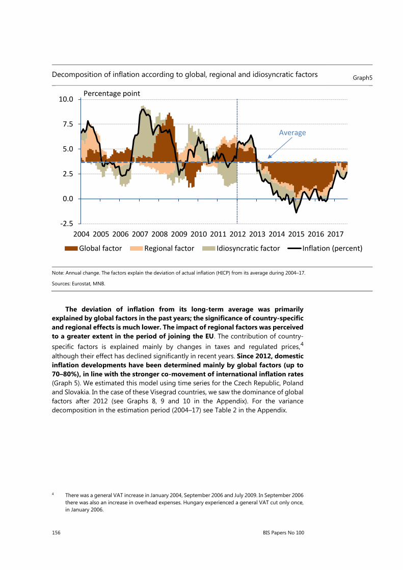
156 BIS Papers No 100
Decomposition of inflation according to global, regional and idiosyncratic factors Graph5
Note: Annual change. The factors explain the deviation of actual inflation (HICP) from its average during 2004–17.
Sources: Eurostat, MNB.
The deviation of inflation from its long-term average was primarily explained by global factors in the past years; the significance of country-specific and regional effects is much lower. The impact of regional factors was perceived to a greater extent in the period of joining the EU. The contribution of country-specific factors is explained mainly by changes in taxes and regulated prices,4 although their effect has declined significantly in recent years. Since 2012, domestic inflation developments have been determined mainly by global factors (up to 70–80%), in line with the stronger co-movement of international inflation rates (Graph 5). We estimated this model using time series for the Czech Republic, Poland and Slovakia. In the case of these Visegrad countries, we saw the dominance of global factors after 2012 (see Graphs 8, 9 and 10 in the Appendix). For the variance decomposition in the estimation period (2004–17) see Table 2 in the Appendix.
4 There was a general VAT increase in January 2004, September 2006 and July 2009. In September 2006
there was also an increase in overhead expenses. Hungary experienced a general VAT cut only once, in January 2006.
-2.5
0.0
2.5
5.0
7.5
10.0
2004 2005 2006 2007 2008 2009 2010 2011 2012 2013 2014 2015 2016 2017
Global factor Regional factor Idiosyncratic factor Inflation (percent)
Percentage point
Average

BIS Papers No 100 157
Identifying the external drivers of domestic inflation using a SVAR approach
To identify the external drivers of the Hungarian inflation, we applied a two-step estimation method on disaggregated inflation data.5 First, we estimated a SVAR model to get the time series of the selected external shocks. Second, we regressed the disaggregated price indices of the main inflation groups on the identified global shocks and on some domestic variables controlling for the prevailing inflation target of the MNB. Finally, we constructed the overall external and internal – or domestic – effects on Hungarian inflation by excluding regulated prices and the effect of indirect taxes.6
We made the estimation using quarterly frequency data – both levels7 and quarterly changes – between Q1 2003 and Q2 2017. As mentioned in Section 1, the external environment in the case of Hungary is the European Union, or rather the euro area. In order to estimate the impact of external shocks, we formed a model with variables reflecting the euro area cyclical position (as a demand shock), global commodity prices (as a commodity-specific shock), euro area inflation (as a supply shock) and interest rates in the euro area (as a monetary policy or interest rate shock). The variable used to capture the external demand shock was the output gap of the euro area based on the European Commission’s estimation.
The four-dimensional Bayesian SVAR model with one period lag was estimated using sign restrictions (Appendix, Table 3) according to the statistical method developed by Dieppe et al (2016). These sign restrictions were needed to avoid infringing the classical economic relationships between demand and supply changes, or between inflation and interest rates. The results of the estimation – the time series of the external shocks and the impulse responses – can be seen in the Appendix (Graphs 11 and 12).
After we obtained the time series of the external shock variables, we formed different OLS-regression models in the case of the main inflation groups: food, industrial goods, services and fuel. The equation stated with estimated external shocks for domestic inflation of the selected groups:
𝜋𝜋𝑖𝑖,𝑡𝑡 = 𝑐𝑐 + 𝛽𝛽1𝜋𝜋𝑖𝑖,𝑡𝑡−1 + 𝛽𝛽2𝑒𝑒𝐷𝐷 + 𝛽𝛽3𝑒𝑒𝐶𝐶 + 𝛽𝛽4𝑒𝑒𝑆𝑆 + 𝛽𝛽5𝑒𝑒𝑅𝑅 + 𝛽𝛽6𝛾𝛾𝑡𝑡−ℎ + 𝛽𝛽7𝜋𝜋𝑡𝑡𝑒𝑒 + 𝜀𝜀𝑡𝑡 (2.)
where 𝜋𝜋𝑖𝑖,𝑡𝑡 is the quarterly inflation in the 𝑖𝑖-th group, 𝑐𝑐 is the constant in the case of food, industrial goods and fuel, and the prevailing inflation target of the central bank in the case of services. The external demand, commodity-specific, supply and interest rate shocks are indicated by 𝑒𝑒𝐷𝐷, 𝑒𝑒𝐶𝐶 , 𝑒𝑒𝑆𝑆 and 𝑒𝑒𝑅𝑅. The variable 𝛾𝛾𝑡𝑡−ℎ indicates the cyclical position of Hungary. This is the output gap for the industrial goods, and the consumption gap in the case of food and services. The lag of the gap variable (ℎ) was chosen to maximise the average adjusted R2 across the regressions. According to the
5 A similar estimation method was used by Hałka and Kotłowski (2016) on Czech, Polish and Swedish
inflation data.
6 We have chosen this inflation indicator because indirect taxes and regulated prices depend on government decisions, which we cannot explain either as an external or internal variable.
7 In the case of the output gap and the service sector’s expectations.

158 BIS Papers No 100
estimations ℎ = 3 was the best choice. In the equation, 𝜋𝜋𝑡𝑡𝑒𝑒 represents Hungarian domestic inflation expectations, or in the case of services the service sector’s expectations.
In all of the regressions we used only the significant explanatory variables at 15% significance level. After that we were able to decompose our inflation indicator. Graph 6 shows the decomposition of Hungary’s external and domestic inflation drivers.
The decomposition of inflation drivers Graph 6
Note: The inflation indicator is the quarterly change in inflation excluding regulated prices and the effect of indirect taxes. External drivers are the effects of shocks to external demand, commodity prices, supply and interest rates. Internal drivers include the effects of domestic slack and domestic inflation expectations.
Source: MNB.
In Graph 6, we can see the average effects of external and internal drivers on the average quarterly change of inflation during 2003–17. Over the whole sample, the effect of the external drivers is stronger than the effect of the internal drivers on inflation. The whole sample can be divided into two subsamples: between 2004 and 2011 the ratio of the effect of both drivers on inflation is nearly equal, but after 2012, the dominance of external drivers is obvious – their weight is more than twice as much as that of the domestic drivers (Table 1). These results are in line with the literature and the results of our PCA estimation.
-0.6-0.5-0.4-0.3-0.2-0.10.00.10.20.30.4
2003 2004 2005 2006 2007 2008 2009 2010 2011 2012 2013 2014 2015 2016 2017
Percentage point
External drivers of inflation Internal drivers of inflation
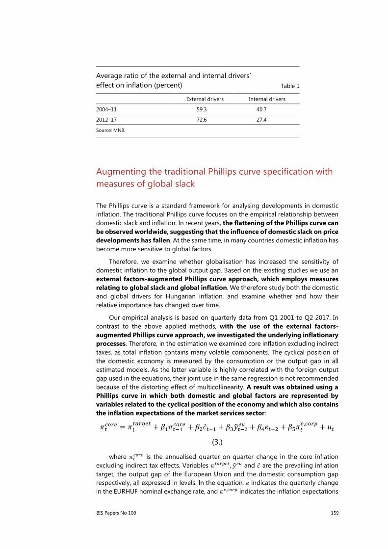
BIS Papers No 100 159
Augmenting the traditional Phillips curve specification with measures of global slack
The Phillips curve is a standard framework for analysing developments in domestic inflation. The traditional Phillips curve focuses on the empirical relationship between domestic slack and inflation. In recent years, the flattening of the Phillips curve can be observed worldwide, suggesting that the influence of domestic slack on price developments has fallen. At the same time, in many countries domestic inflation has become more sensitive to global factors.
Therefore, we examine whether globalisation has increased the sensitivity of domestic inflation to the global output gap. Based on the existing studies we use an external factors-augmented Phillips curve approach, which employs measures relating to global slack and global inflation. We therefore study both the domestic and global drivers for Hungarian inflation, and examine whether and how their relative importance has changed over time.
Our empirical analysis is based on quarterly data from Q1 2001 to Q2 2017. In contrast to the above applied methods, with the use of the external factors-augmented Phillips curve approach, we investigated the underlying inflationary processes. Therefore, in the estimation we examined core inflation excluding indirect taxes, as total inflation contains many volatile components. The cyclical position of the domestic economy is measured by the consumption or the output gap in all estimated models. As the latter variable is highly correlated with the foreign output gap used in the equations, their joint use in the same regression is not recommended because of the distorting effect of multicollinearity. A result was obtained using a Phillips curve in which both domestic and global factors are represented by variables related to the cyclical position of the economy and which also contains the inflation expectations of the market services sector:
𝜋𝜋𝑡𝑡𝑐𝑐𝑐𝑐𝑐𝑐𝑒𝑒 = 𝜋𝜋𝑡𝑡𝑡𝑡𝑡𝑡𝑐𝑐𝑡𝑡𝑒𝑒𝑡𝑡 + 𝛽𝛽1𝜋𝜋𝑡𝑡−1𝑐𝑐𝑐𝑐𝑐𝑐𝑒𝑒 + 𝛽𝛽2�̂�𝑐𝑡𝑡−1 + 𝛽𝛽3𝑦𝑦�𝑡𝑡−2𝑒𝑒𝑒𝑒 + 𝛽𝛽4𝑒𝑒𝑡𝑡−2 + 𝛽𝛽5𝜋𝜋𝑡𝑡
𝑒𝑒,𝑐𝑐𝑐𝑐𝑐𝑐𝑐𝑐 + 𝑢𝑢𝑡𝑡
(3.)
where 𝜋𝜋𝑡𝑡𝑐𝑐𝑐𝑐𝑐𝑐𝑒𝑒 is the annualised quarter-on-quarter change in the core inflation excluding indirect tax effects. Variables 𝜋𝜋𝑡𝑡𝑡𝑡𝑐𝑐𝑡𝑡𝑒𝑒𝑡𝑡 ,𝑦𝑦�𝑒𝑒𝑒𝑒 and �̂�𝑐 are the prevailing inflation target, the output gap of the European Union and the domestic consumption gap respectively, all expressed in levels. In the equation, 𝑒𝑒 indicates the quarterly change in the EURHUF nominal exchange rate, and 𝜋𝜋𝑒𝑒,𝑐𝑐𝑐𝑐𝑐𝑐𝑐𝑐 indicates the inflation expectations
Average ratio of the external and internal drivers’ effect on inflation (percent) Table 1
External drivers Internal drivers
2004–11 59.3 40.7
2012–17 72.6 27.4
Source: MNB.

160 BIS Papers No 100
of the market services sector, capturing the forward-looking nature of our Phillips curve specification.
The strengthening role of external factors is confirmed by a rolling window estimation of the Phillips curve (Graph 7). The coefficient of the domestic consumption gap is not significant in most of the cases, suggesting that country-specific effects are losing their importance in core inflation processes. This is in line with the flattening of the Phillips curve estimated using Hungarian data for the period following the crisis. For the whole sample, the coefficient of the EU output gap – capturing global effects – is significantly stronger than the coefficient of the domestic consumption gap, ie domestic inflation is more sensitive to global factors. Based on the estimation, if the output gap of the European Union increases by 1 percentage point, core inflation without tax effects increases by 0.1–0.2 percentage points (Appendix, Table 4). In order to check the robustness of the results, further specifications were estimated, which resulted in similar coefficients concerning the role of external factors (Appendix, Table 5).
Rolling window estimation – changes in the coefficients of the domestic consumption gap (left panel) and the EU output gap (right-hand panel) estimated for domestic core inflation Graph 7
Note: The seven-year rolling window regression was estimated on annualised quarterly data. The uncertainty of the estimation indicates one unit of standard deviation.
Sources: European Commission, Eurostat, HCSO, MNB.
Besides OLS estimations the above-specified Phillips curve was also estimated with the generalised method of moments (Hansen (1982)), in order to address the risk of endogeneity of some explanatory variables.8 We consider four lags
8 Similar estimations were made by Mikolajun and Lodge (2016) for 19 advanced economies, but they
found little support for the existence of direct effects of global economic slack on domestic inflation.
-0.2-0.10.00.10.20.30.40.50.60.70.8
2002
–08
2003
–09
2004
–10
2005
–11
2006
–12
2007
–13
2008
–14
2009
–15
2010
–16
-0.2-0.10.00.10.20.30.40.50.60.70.8
2002
–08
2003
–09
2004
–10
2005
–11
2006
–12
2007
–13
2008
–14
2009
–15
2010
–16
BIS Papers No 100 161
of the domestic consumption gap and the EU output gap, three lags of Hungarian inflation expectations and one lag of the EURHUF exchange rate and the core inflation as instruments in the GMM. The lag order is selected based on two information criteria,9 allowing for a maximum lag of four quarters. Heteroskedasticity and Autocorrelation Consistent (HAC) estimates were used with a Bartlett kernel and an automatic Newey–West bandwidth selection. The sensitivity of the domestic inflation to global factors is also confirmed by the GMM estimation. The coefficient of the EU output gap is significant and higher than the coefficient of the domestic consumption gap on the whole sample (Appendix, Table 6).
Conclusion
Inflation rates have been declining at the global level since 2013. As a result of rising commodity prices at end-2016 and in early 2017, inflation rates have moved away from close-to-zero levels, but they have still tended to fall short of central bank targets. Economic performance has varied from region to region after the crisis, which is also corroborated by the significantly different levels of unemployment in the EU. However, despite the different phase of the labour market cycle, no divergence could be detected in inflation dynamics. Indeed, inflation rates have tended to remain at generally low levels in recent years.
The strengthening correlation between inflation rates may be explained by globalisation and integration into global production processes (the role of global value chains), which may have amplified the impact of international business cycles on inflation. Correlation among the price indices of the EU countries has increased considerably in recent years. In the case of Hungary, these are important findings, because the European Union represents the effective global environment, as approximately 80% of Hungary’s foreign trade is with the EU. Since Hungary became extremely open in the last two decades, we examined the impact of external and domestic drivers of the Hungarian inflation, and we analysed how these external factors varied in time and how their effect on the domestic inflation has changed.
On the whole, based on the results of the principal component analysis and the two-step SVAR approach, the role of external factors in domestic inflation developments has recently strengthened, and after 2012, the changes in inflation in Hungary have been influenced mainly by global effects. The growing role of external factors is also confirmed by the changes in the coefficients of the external factors-augmented Phillips curve estimation. This is in line with the flattening of the Phillips curve estimated using Hungarian data for the period following the crisis. For the whole sample, the coefficient belonging to the output gap of the European Union capturing global effects is significantly stronger than the coefficient of the domestic consumption gap, ie domestic inflation is more sensitive to global factors.
9 Schwarz’s information criterion and the Hannan–Quinn information criterion.

162 BIS Papers No 100
Appendix
Decomposition of Czech inflation according to global, regional and idiosyncratic factors Graph 8
Note: Annual change. The factors explain the deviation of actual inflation (HICP) from its average between 2004–17.
Sources: Eurostat, MNB.
-1.4
0.0
1.4
2.8
4.1
5.5
6.9
8.3
2004 2005 2006 2007 2008 2009 2010 2011 2012 2013 2014 2015 2016 2017
Percentage point
Global factor Regional factor Idiosyncratic factor Inflation (percent)
Average

BIS Papers No 100 163
Decomposition of Polish inflation according to global, regional and idiosyncratic factors Graph 9
Note: Annual change. The factors explain the deviation of actual inflation (HICP) from its average between 2004–17.
Sources: Eurostat, MNB.
-2.0
-1.0
0.0
1.1
2.1
3.1
4.1
5.2
6.2
2004 2005 2006 2007 2008 2009 2010 2011 2012 2013 2014 2015 2016 2017
Percentage point
Global factor Regional factor Idiosyncratic factor Inflation (percent)
Average

164 BIS Papers No 100
Decomposition of Slovak inflation according to global, regional and idiosyncratic factors Graph 10
Note: Annual change. The factors explain the deviation of actual inflation (HICP) from its average between 2004–17.
Sources: Eurostat, MNB.
Variance decomposition in the estimation period (2004–17, percent) Table 2
Global factor Regional factor Idiosyncratic factor
Hungary 51 10 39
Czech Republic 76 1 23
Poland 52 7 41
Slovakia 53 2 45
Source: MNB.
-2.2-1.5-0.70.00.81.52.33.03.84.55.36.06.87.58.39.0
2004 2005 2006 2007 2008 2009 2010 2011 2012 2013 2014 2015 2016 2017
Percentage point
Global factor Regional factor Idiosyncratic factor Inflation (percent)
Average

BIS Papers No 100 165
Sign restrictions used in the SVAR estimation Table 3
Variable Euro area output gap Global commodity price index
Euro area HICP Euro area interest rates
Euro area output gap + - - -
Global commodity price index +
Euro area HICP + + + -
Euro area interest rates + +
Source: MNB.
Shocks of the SVAR estimation Graph 11
Source: MNB.
-4.5
-3.0
-1.5
0.0
1.5
3.0
2003
2004
2005
2006
2007
2008
2009
2010
2011
2012
2013
2014
2015
2016
2017
Euro area demand shock
-2.0
-1.0
0.0
1.0
2.0
2003
2004
2005
2006
2007
2008
2009
2010
2011
2012
2013
2014
2015
2016
2017
Euro area supply shock
-2.5-2.0-1.5-1.0-0.50.00.51.01.52.02.5
2003
2004
2005
2006
2007
2008
2009
2010
2011
2012
2013
2014
2015
2016
2017
Global commodity-specific shock
-1.5-1.0-0.50.00.51.01.5
2003
2004
2005
2006
2007
2008
2009
2010
2011
2012
2013
2014
2015
2016
2017
Euro area interest rate shock

166 BIS Papers No 100
Impulse responses of euro area variables to external shocks Graph 12
-0.6
-0.4
-0.2
0.0
0.2
1 2 3 4 5 6 7 8 9 10
Percentage pointOutput gap to commodity shocks
-0.2
0.0
0.2
0.4
0.6
1 2 3 4 5 6 7 8 9 10
Percentage pointOutput gap to demand shocks
-2
0
2
4
6
8
1 2 3 4 5 6 7 8 9 10
Percentage pointCommodity prices to demand shocks
-0.05
0.00
0.05
0.10
0.15
1 2 3 4 5 6 7 8 9 10
Percentage pointEA HICP-inflation to demand shocks
0.0
0.1
0.2
0.3
0.4
0.5
1 2 3 4 5 6 7 8 9 10
Percentage pointEA interest rates to demand shocks
-2
0
2
4
6
8
1 2 3 4 5 6 7 8 9 10
Percentage pointCommodity prices to commodity shocks
-0.05
0.00
0.05
0.10
0.15
1 2 3 4 5 6 7 8 9 10
Percentage pointEA HICP-inflation to commodity shocks
-0.4-0.3-0.2-0.10.00.10.2
1 2 3 4 5 6 7 8 9 10
Percentage pointEA interest rates to commodity shocks
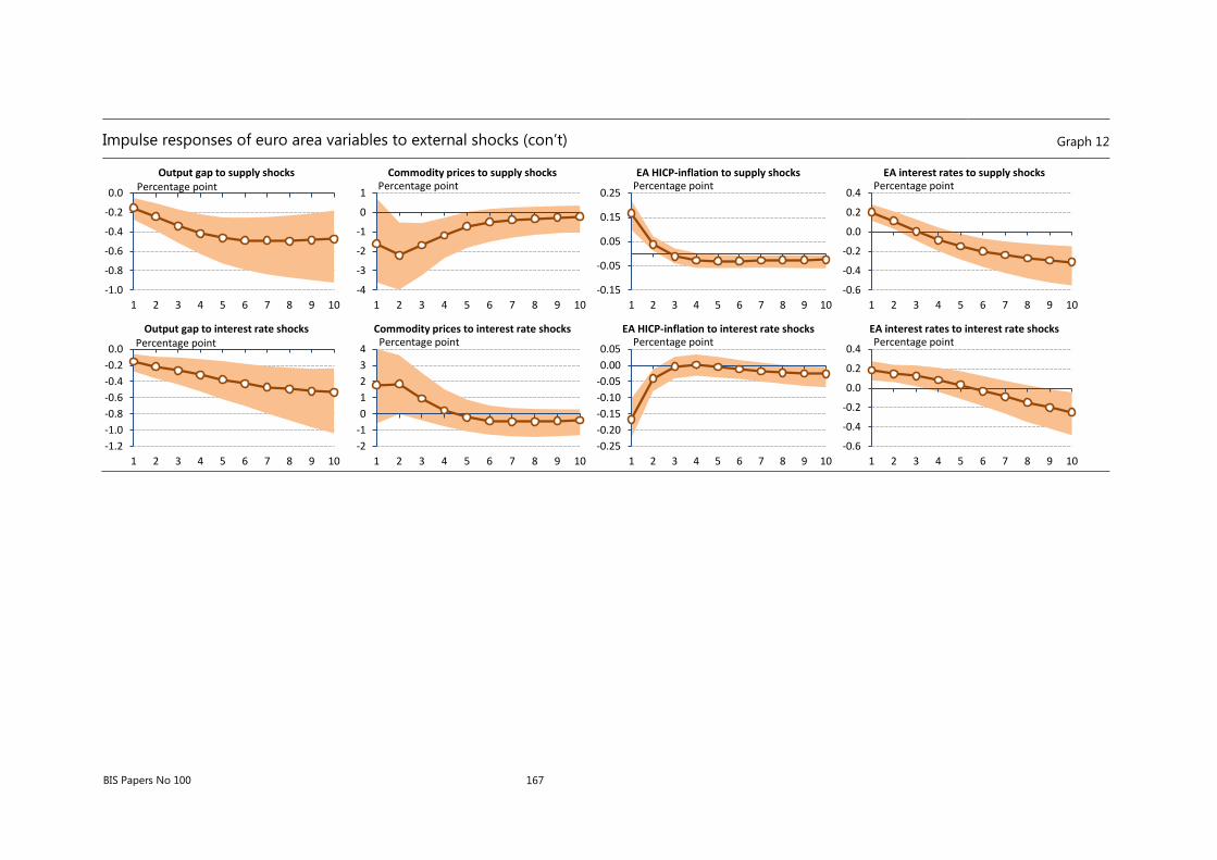
BIS Papers No 100 167
Impulse responses of euro area variables to external shocks (con’t) Graph 12
-1.0
-0.8
-0.6
-0.4
-0.2
0.0
1 2 3 4 5 6 7 8 9 10
Percentage pointOutput gap to supply shocks
-4
-3
-2
-1
0
1
1 2 3 4 5 6 7 8 9 10
Percentage pointCommodity prices to supply shocks
-0.15
-0.05
0.05
0.15
0.25
1 2 3 4 5 6 7 8 9 10
Percentage pointEA HICP-inflation to supply shocks
-0.6
-0.4
-0.2
0.0
0.2
0.4
1 2 3 4 5 6 7 8 9 10
Percentage pointEA interest rates to supply shocks
-1.2-1.0-0.8-0.6-0.4-0.20.0
1 2 3 4 5 6 7 8 9 10
Percentage pointOutput gap to interest rate shocks
-2-101234
1 2 3 4 5 6 7 8 9 10
Percentage pointCommodity prices to interest rate shocks
-0.25-0.20-0.15-0.10-0.050.000.05
1 2 3 4 5 6 7 8 9 10
Percentage pointEA HICP-inflation to interest rate shocks
-0.6
-0.4
-0.2
0.0
0.2
0.4
1 2 3 4 5 6 7 8 9 10
Percentage pointEA interest rates to interest rate shocks

168 BIS Papers No 100
The specification of our baseline Phillips curve estimation Table 4
Explanatory variables Coefficient Std. Error
Inflation target 0.43*** 0.11
Core inflation excluding indirect taxes (–1) 0.36*** 0.12
Consumption gap (-1) 0.09* 0.06
Output gap of the European union (–2) 0.15* 0.10
HUF/EUR exchange rate (–2) 0.02* 0.01
Inflation expectations 0.04* 0.02
R2 0.62
Akaike information criterion 2.89
Schwarz information criterion 3.11
Note: Number of lags in parenthesis after the names of the explanatory variables. *, ** and *** denote statistical significance at 15%, 5% and 1% levels.
Sources: European Commission, Eurostat, HCSO, MNB.
The specification of our alternative Phillips curve estimations Table 5
Model 1 Model 2 Model 3 Model 4
Inflation target 0.09 (0.10) 0.35 (0.09)*** 0.10 (0.09) 0.26 (0.10)**
Core inflation excluding indirect taxes (-1) 0.49 (0.10)*** 0.56 (0.11)*** 0.37 (0.11)*** 0.21 (0.13)*
Consumption gap (–1) 0.08 (0.06)
Consumption gap (–2) 0.11 (0.06)*
Consumption gap (–3) 0.06 (0.05)
Domestic output gap (–3) 0.08 (0.07)
Core inflation of the EU 0.85 (0.23)*** 0.81 (0.21)***
Core inflation of the EU (–1) 0.65 (0.28)**
Output gap of the EU (–2) 0.16 (0.08)*
EURHUF exchange rate (–1) 0.03 (0.01)*** 0.03 (0.01)*** 0.03 (0.01)***
EURHUF exchange rate (–2) 0.02 (0.01)**
Inflation expectations 0.04 (0.02)*** 0.05 (0.02)***
R2 0.70 0.67 0.73 0.65
Akaike information criterion 2.63 2.76 2.55 2.81
Schwarz information criterion 2.80 2.93 2.76 3.03
Note: Number of lags in parenthesis after the names of the explanatory variables. *, ** and *** denote statistical significance at 15%, 5% and 1% levels.
Source: European Commission, Eurostat, HCSO, MNB

BIS Papers No 100 169
GMM estimates of the Phillips curve Table 6
Explanatory variables Coefficient Std. Error
Intercept 2.12*** 0.24
Consumption gap (–1) 0.18*** 0.05
Output gap of the European Union (–2) 0.22** 0.1
Inflation expectations 0.06*** 0.02
EURHUF exchange rate (–2) 0.04*** 0.01
P-value of the J-test 0,86
R-squared 0,59
Number of observations 55
Note: Dependent variable is core inflation excluding indirect tax effects. GMM estimation. Instruments include four lags of the domestic consumption gap and the EU output gap, three lags of the Hungarian inflation expectations, one lag of EURHUF exchange rate, and one lag of the core inflation. *, ** and *** denote statistical significance at 15%, 5% and 1% levels.
Sources: European Commission, Eurostat, HCSO, MNB.

170 BIS Papers No 100
References
Auer, R, A Levchenko and P Sauré (2017): “International inflation synchronisation through global value chains”, VoxEU.org, 19 May.
Bean, C (2006): “Impact of globalization on monetary policy: Commentary”, comments delivered at the Jackson Hole Economic Policy Symposium, Jackson Hole, Wyoming (an event sponsored by the Federal Reserve Bank of Kansas City) and published in the Proceedings of the Economic Policy Symposium, 26 August, pp 307–16.
Bernanke, B (2007): “Globalization and monetary policy”, speech at the Fourth Economic Summit, Stanford Institute for Economic Policy Research, 2 March.
Borio, C (2017): “How much do we really know about inflation?”, speech at the Bank’s 87th Annual General Meeting, Basel, 25 June.
Borio, C and A Filardo (2007): “Globalisation and inflation: New cross-country evidence on the global determinants of domestic inflation”, BIS Working Papers, no 227.
Borio, C, R Auer and A Filardo (2017): “The globalisation of inflation: the growing importance of global value chains”, BIS Working Papers, no 602.
Bulligan, G and E Viviano (2016): “Has the wage Phillips curve changed in the euro area?”, Bank of Italy Occasional Papers, no 355, September.
Calza, A (2008): “Globalisation, domestic inflation and global output gaps: evidence from the euro area”, Federal Reserve Bank of Dallas, Working Paper, no 13.
Carney, M (2015): Remarks delivered at the Jackson Hole Economic Policy Symposium, Jackson Hole, Wyoming (an event sponsored by the Federal Reserve Bank of Kansas City) and published in the Proceedings of the Economic Policy Symposium, 29 August, pp 437–54.
Caruana, J (2012): Speech at the CEMLA-SEACEN conference on “The role of central banks in macroeconomic and financial stability: the challenges in an uncertain and volatile world”, Punta del Este, Uruguay, 16 November.
Ciccarelli, M and B Mojon (2005): “Global inflation”, ECB Working Paper Series, no 537, October.
——— (2010): “Global inflation”, Review of Economics and Statistics, vol 92, no 3, August, pp 524–35.
Draghi, M (2016): “How central banks meet the challenge of low inflation”, Marjolin Lecture, Frankfurt, 4 February.
Dieppe, A, R Legrand and B van Roye (2016): “The BEAR toolbox”, ECB Working Paper Series, no 1934, July.
ECB (2017): Economic Bulletin, issue 4.
Eickmeier, S and K Pijnenburg (2013): “The global dimension of inflation – evidence from factor-augmented Phillips curves”, Oxford Bulletin of Economics and Statistics, vol 75, no 1, pp 103–22.
BIS Papers No 100 171
Fischer, S (2015): “US inflation developments”, speech delivered at the Jackson Hole Economic Policy Symposium, Jackson Hole, Wyoming (an event sponsored by the Federal Reserve Bank of Kansas City), 29 August.
Fisher, R (2006): “Coping with globalization’s impact on monetary policy”, speech at the Allied Social Science Association Meetings, Boston, 6 January.
Gerlach, S, A Giovannini, C Tille and J Vinals (2008): “Low inflation: testing times for central banks”, 10th Geneva Report on the World Economy.
Guerrieri, L, C Gust and J López-Salido (2010): “International competition and inflation: a new Keynesian perspective”, American Economic Journal: Macroeconomics, vol 2, no 4, pp 247–80.
Hałka, A and J Kotłowski (2016): “Global or domestic? Which shocks drive inflation in European small open economies?”, NBP Working Papers, no 232, Narodowy Bank Połski.
Hansen, L (1982): “Large sample properties of generalized method of moments estimators”, Econometrica, vol 50, no 4, pp 1029–54.
Ihrig, J, S Kamin, D Lindner and J Marquez (2010): “Some simple tests of the globalisation and inflation hypothesis”, International Finance, vol 13, no 3, pp 343–75.
Jordan, T (2015): “The impact of international spillovers on Swiss inflation and the exchange rate”, Journal of International Money and Finance, vol 68, no 1, pp 262–65.
Krusper, B (2012) “The role of external and country specific factors in Hungarian inflation developments”, MNB Working Papers, no 2012/5, Magyar Nemzeti Bank.
Martínez-García, E and M Wynne (2010): “The global slack hypothesis”, Federal Reserve Bank of Dallas, Staff Papers, no 10.
Mikolajun, I and D Lodge (2016): “Advanced economy inflation: the role of global factors”, ECB Working Papers, no 1948.
Milani, F (2009): “Global slack and domestic inflation rates: a structural investigation for G-7 countries”, Federal Reserve Bank of Dallas, Working Papers, no 33.
Magyar Nemzeti Bank (2017): Inflation Report, September, pp 61–64.
Morimoto, Y, W Hirata and R Kato (2003): “Global disinflation”, Bank of Japan Research Papers, no 2003/06/13, June.
Mumtaz, H and P Surico (2008): “Evolving international inflation dynamics: world and country specific factors”, Bank of England Working Papers, no 341.
Muto, I and K Shintani (2014): “An empirical study on the New Keynesian wage Phillips curve: Japan and the US”, Bank of Japan Working Paper Series, no 14-E-4, February.
Nickel, C (2017): “The role of foreign slack in domestic inflation in the Eurozone”, VoxEU.org, 28 July.
Poloz, S (2016): “Cross-border trade integration and monetary policy”, The Paul Storer Memorial Lecture, delivered at Western Washington University, Bellingham, Washington, 26 September.
Stock, J and M Watson (2002): “Macroeconomic forecasting using diffusion indexes”, Journal of Business and Economic Statistics, vol 20, no 2, April, pp 147–62.

172 BIS Papers No 100
Yellen, J (2006): Speech delivered at the “Euro and the dollar in a globalized economy” conference, Federal Reserve Bank of San Francisco, 27 May.

BIS Papers No 100 173
Globalisation and deglobalisation: the Indonesian perspective
Dody Budi Waluyo, Deputy Governor, Bank Indonesia
Abstract
Globalisation has created new opportunities for both advanced and emerging economies. In the case of Indonesia, the country’s integration with world markets has correlated positively and strongly with economic growth. Foreign direct investment has supported a shift to higher value added industries, while total factor productivity growth has also tended to benefit from globalisation. The effects on the labour market have also been positive.
However, globalisation and increasing trade openness also have unintended consequences, in that the economy becomes more susceptible to global economic and financial cycles. Supply chains between Asian countries become the pass-through channel for any global shocks to price instability, particularly those related to production costs. Meanwhile, increasing automation in some sectors, the growing skill premium, and rising employment in the informal have contributed to growing inequality.
To realise the full benefits of globalisation, domestic authorities should focus on maintaining the domestic economy’s soundness and competitiveness. By improving their policy coordination and strengthening risk management, national authorities should seek to create systemic resilience in withstanding bouts of uncertainty and volatility from open economic and financial markets.
Keywords: Globalisation, trade openness, international trade.
JEL classification: F13, F15.
174 BIS Papers No 100
Globalisation is defined as integration into international capital, commodity and labour markets (Bordo (2003)). Therefore, the focus of globalisation is not only on international trade in goods and international movements of capital (including foreign investment, portfolio flows and aid), but also on cross-country migration and trade in services that are associated with labour market dynamics and skills/technology transfer. Baldwin and Martin (1999) identify two episodes of globalisation, the first starting around the mid-19th century and continuing until World War I, and the second starting after World War II and continuing today.
Determinants of globalisation
Globalisation has created new opportunities for both advanced and emerging economies. Economic globalisation in Indonesia started after the end of World War II, driven by international trade and industrialisation. Indonesia’s latest trade figures show the effects of globalisation. In 2016, exports amounted to USD 144.7 billion and imports to USD 135.6 billion, resulting in a positive trade balance of USD 8.9 billion, making Indonesia the world’s 26th largest exporter. The top three Indonesian exports are mineral fuels, mineral oils and products of their distillation (USD 27 billion), animal or vegetable fats and oils and their cleavage products (USD 18.3 billion), and electrical machinery and equipment and parts (USD 8.15 billion). The top three imports are machinery and mechanical appliances (USD 21 billion), mineral fuels and products of their distillation (USD 19 billion), and electrical machinery and equipment and parts (USD 15 billion). This trade performance is supported by structural transformations in agriculture as well as the manufacturing and service sectors.
From the mid-1960s to the 1980s, Indonesia was able to reap the first benefits from worldwide investment flows, knowledge exchange and rapid economic growth. During 1975–80, Indonesia’s economy grew by 7.5% annually on average. Over the next five years, growth slowed to 3.7% annually. In response, the country altered its trade regime to become more outward looking. The effect was to increase the integration of Indonesia into the global economy through trade and financial flows.
The second driver of globalisation was industrialisation. In general, developing countries frequently lack the conditions to support the process of industrialisation. Capital is limited since the saving rate is still relatively low, and there are shortages of both technology and skilled human resources. This encourages the inward flow of capital, either through foreign direct investment (FDI) or the flow of funds to domestic portfolio instruments, and the flow of skilled workers (migration) from developed countries. A strategy of integrating with global value chains is also seen as part of this industrialisation agenda. As a developing country with a lower level of technology and abundant low-skill labour resources, Indonesia was able to reap the benefits of industrialisation as multinational companies moved production there.
Many believe that globalisation has a positive impact on both advanced and emerging countries. Globalisation optimises resource allocation, so that global output is higher than it would be without global economic integration. Therefore, countries will continue to expand their exposure to global markets through globalisation even if protectionism is an inevitable side effect of the recent rise in
BIS Papers No 100 175
political populism. However, this effect is expected to be temporary since there is not yet any evidence of net benefits from protectionism in the global context.
Macroeconomic effects of globalisation
Globalisation has generally promoted economic growth. Using data on the economic growth of ASEAN countries between 1970 and 2008 and the KOF Index of Globalisation, Ying et al (2014) find that globalisation has increased economic growth in ASEAN countries, including Indonesia. Their results indicate that an increase in globalisation of approximately 1 percentage point lifts economic growth by 1.48%, in particular due to technological advances. A similar result was obtained by Dreher (2005), who noted that economic integration via globalisation promotes higher economic growth.
China’s role in the global economy has greatly increased in the decade since the Asian financial crisis. China’s ascent has been driven by its export-led growth policy since joining the WTO in 2001. Mass production of manufactured consumption goods has boosted China’s economic growth and also created spillovers to neighbouring regions that provide raw materials. Indonesia, Malaysia and the Philippines are among the beneficiaries of China’s high economic growth, particularly through commodities exports. Along with trade expansion, the flow of investment from China has also increased exponentially.
Trade integration as a measure of trade openness (trade as percentage of GDP) has had a positive and strong correlation with economic growth in Indonesia, particularly after the Great Financial Crisis (GFC) in 2008. Trade openness increased from 22% in the 1960s to around 60% in the 1990s, although it stabilised after the Asian crisis in 1998 and declined following the GFC to 37% in 2016. The acceleration of economic openness was accompanied by regulatory reform in trade policy focused on bolstering economic growth. Using a plant-level panel data set from the Indonesian manufacturing sector, Takii and Narjoko (2013) study the impact of globalisation through trade liberalisation on the size of plants as measured by real output. The paper finds that foreign-owned firms which participate in international activities have scale advantages.
Regarding foreign direct investment (FDI), Sjöholm (2016) documents the impact of FDI on Indonesia and finds that foreign firms generate higher value added, which in turn spills over to domestic firms’ value added. Therefore, FDI promotes structural change via higher value added industry, boosting investment, tax revenues and wages. Eventually, this process should foster both economic growth and improved living standards. Thus, globalisation through FDI reduces not only the productivity gap but also the wage differential between developing and advanced economies.
In terms of total factor productivity (TFP) growth, ASEAN economies, including Indonesia, tend to perform relatively well during globalisation. Consistent with existing evidence, TFP growth in manufacturing tends to outpace that in services for most economies. The productivity growth of Asian economies, in particular of the service sector, is sometimes lower than that of the manufacturing sector (McGregor et al (2017)). Using a sample of 40 economies during the period 1995–2009, the paper found that total factor productivity (TFP) growth in Asian

176 BIS Papers No 100
economies has been relatively strong compared with that of other countries. Particularly in Indonesia, most of the GDP growth was explained by the growth in the capital stock as well as the growth of education-adjusted employment.
However, globalisation and increasing trade openness have unintended consequences for emerging market economies since the economy has become more responsive to the global economic and financial cycle. Closer trade connections increase the economy’s sensitivity to inflation. Recently, there has been a notable convergence of Asia-Pacific’s inflation levels, particularly in terms of consumer prices, induced by an increasing share of these economies’ trade in total international trade.
As domestic supply chains between Asian countries have become increasingly integrated, they have become the pass-through channel for global shocks, particularly those related to production costs. Trade intensity in Asian economies is empirically associated with the co-movement of inflation rates. Baldwin (2013) finds that a one standard deviation increase in trade intensity between two economies is associated with a roughly 3–6 percentage point increase in the correlation between the consumer price index inflation rates of the same economies. The trade intensity factor remains robust even after control variables are included.
In addition, economic growth dynamics are changing, particularly for commodity exporters. Indonesia’s economic growth has moved more or less in line with China’s business cycle since the beginning of the commodity boom. In Asia, China is the main importer of commodities. The positive correlation between Indonesia’s and China’s business cycles was more significant during the commodity boom from 2006 to 2013. China’s influence is also felt in the form of capital inflows through real investment in the manufacturing, mining and services sector. A more synchronised business cycle also poses the risk of a negative spillover from any slowdown in China, which would impact not only on commodities exports from emerging markets, but also on exports of intermediate goods for manufacturing. Although China accounts for only 13% of Indonesia’s total exports, it is the main market for exports of coal, palm oil and various metals, and hence the effects spread across several economic sectors.
Moreover, the surge of commodities exports in the last decade has transformed Indonesia’s economic structure. Total exports from Indonesia amounted to USD 144.7 billion in 2016, which were dominated by exports of mineral fuels, mineral oils and their distillation products (USD 27 billion), as well as animal or vegetable fats and oils and their cleavage products (USD 18.3 billion). Exports of electrical machinery and equipment and parts accounted for USD 8.15 billion in 2016. Back in 1993, the share of the industrial sector was about 27%, but this had fallen to 21.4% by the last quarter of 2016. The decline in the share of manufacturing over the past 15 years is quite significant for an emerging market economy like Indonesia’s that aims to attain upper middle income levels through robust industrialisation and the creation of quality jobs.
The falling share of the manufacturing sector in Indonesia’s economy is also related to rising commodity prices, which have driven an appreciation of the currency and thus put pressure on the competitiveness of the industrial sector. This has reduced the incentive for the manufacturing sector to invest in improved technology, R&D and worker skills. Given insufficient skills, capacity and capability, the labour force is limited to low-skilled jobs. As a result, most of the workforce in the primary sector (agriculture and mining) is shifting to the low-skilled services sector,

BIS Papers No 100 177
which has grown rapidly in line with rising domestic consumption. Unfortunately, owing to the lack of innovation and applied technology, productivity in the services sector is relatively low.
The recent episode of globalisation was a period of technological advancement. In particular, the internet has helped emerging market economies join the digital economy. The growth of e-commerce has flourished in the past two years. In Indonesia, for example, Go-jek is a technology company that focuses on providing online transportation services with plans to expand into fintech services. Innovation and increased productivity could further drive the integration of emerging market economies into the global economy.
Distributional effects of globalisation
Besides its macroeconomic effects, increased domestic economic integration with the global economy also has an impact on the labour market. Globalisation impacts positively on the labour market as working conditions have improved, especially in manufacturing. Increased integration of labour markets has also reduced the wage gap among workers in advanced and emerging market economies. Sitalaksmi et al (2007) use individual employment data to argue that the increase in export-oriented foreign direct investment influenced relative wages in the textile and apparel sector. Additionally, working conditions, proxied by workers’ own assessment of their income, working facilities, medical benefits, safety considerations and transport opportunities, have improved over time in the expanding manufacturing industries as compared with agriculture.
Existing studies on the effects of Indonesian trade liberalisation show both increased firm productivity and improvements in working conditions in manufacturing. At the plant level, Amiti and Konings (2007) find that trade liberalisation affected firms’ productivity via two channels: falling tariffs on imported inputs fostered learning and raised both product quality and variety, while falling output protection increased competitive pressures. Comparing the two effects, the paper argues that the gains from falling input tariffs were considerably higher. Firm productivity also has been strongly affected by FDI flows, as firms with increasing foreign ownership experienced restructuring, employment and wage growth, as well as stronger linkages to export and import markets (Arnold and Smarzynska Javorcik (2005)). However, regional autonomy, issues relating to local governance, infrastructure and uncertainties in local regulations are increasingly important as well as some programmes that promote specific locations as special economic zones to attract manufacturing investors.
The trend to automation in a number of sectors also has an impact on growing inequality. Automation in the manufacturing sector has caused job losses, especially among unskilled workers. In the trade sector, unskilled workers are also being affected by the growth of the digital economy (e-commerce), which tends to eliminate jobs. The types of job created by the digital economy are also limited to mostly higher-skilled workers. Even though jobs growth remains relatively stable, the growth of formal jobs has continued to decline after the GFC. Meanwhile the number of informal jobs has grown slightly. This is a concern since lower-quality jobs imply lower wages.
178 BIS Papers No 100
The increasing trend towards a skill premium has contributed to rising wage inequality. Globalisation has slightly increased the skill premium (wage differences between skilled and unskilled workers). Goldberg and Pavcnik (2007) found that, during globalisation, a shift in demand for skilled workers expands skill premia. Using data from medium and large Indonesian manufacturing firms covering the 2000–08 period, Takii and Narjoko (2013) find that there is a declining pattern in relative wages (skilled vs unskilled), with a slight increase in the trend towards skilled employment. They also found that plants involved with international trade and/or with foreign ownership pay higher wages to their skilled workers and employ more skilled workers compared with local and domestic-oriented plants. However, the latest research conducted by Amiti and Cameron (2012), which revealed the extent of the skill premium in the wake of globalisation, could not find any definite pattern, either between industries or over time. But a study by Suryahadi (2001) finds a fast increase in the employment of skilled labour as well as a decline in wage inequality (faster wage growth for the unskilled) in parallel with Indonesia’s trade liberalisation.
Increased informal sector employment has also aggravated inequality. Since more individuals in developing countries are not employed in the formal labour market, but instead work in the informal sectors such as household businesses and family farms (Rosenzweig (1988)), thus potentially expanding wealth inequality. Goldberg and Pavcnik (2007) concluded that globalisation affects individuals through three main channels, namely, changes in labour income, changes in relative prices and consumption, and changes in household production decisions.
Policy implications
Even though it is not yet fully clear who will be the ultimate winners and the losers from globalisation, several studies have outlined which sectors and workers have benefited most to date. More educated people (skilled workers) have benefited more from integrated global trade. The same is true of the more capital and technologically intensive manufacturing sectors as compared with more labour-intensive manufacturing sectors.
For emerging market economies, globalisation brings new opportunities to increase economic growth and productivity, but also creates new challenges for authorities. Simorangkir (2006) shows that failure to anticipate trade openness has undermined the competitiveness of Indonesian products relative to foreign ones, lowering output in the medium to long term. Openness in the financial sector has increased the vulnerability of the Indonesian economy to reversals in capital flows. Trade openness and financial openness are significantly associated with fluctuations in output, exchange rates and inflation in both the very short and long run. Moreover, the benefits of globalisation do not extend equally across countries and sectors.
In order to optimise the benefits from globalisation, authorities should place the emphasis on increasing economic competitiveness. The development of both hard and soft skills is one of the key factors in creating skilled workers and fostering innovation. This type of human resources development strategy, combined with an investment policy to attract high added value and technologically intensive industries linked to global value chains, will maximise the benefits from globalisation. At the same time, increasing domestic connectivity will help to reduce gaps between regions.

BIS Papers No 100 179
Central banks can play a role in helping EMEs reap the benefits of globalisation. First, central banks must commit themselves to preserving macroeconomic stability, including price stability. By preserving macroeconomic stability, central banks help EMEs stabilise output fluctuations, which may be amplified by globalisation, as previously discussed. Second, the inflation process may also change as shocks from other countries are more easily transmitted to the domestic economy. In this case, central banks should continue anchoring inflation expectations at a level that is consistent with central bank’s definition of price stability. The credibility of the central bank will reduce second-round inflationary effects and mitigate fluctuations in output and inflation. Third, central banks should encourage cross-border cooperation, for example, exchanges of information in order to paint a comprehensive picture of risks and vulnerabilities, and coordinate their actions to manage liquidity and ensure the efficient functioning of the interbank money market.
Following the Asian financial crisis, Bank Indonesia has made various efforts to strengthen the risk management and mitigation aspects of the macroeconomic and financial system. For Bank Indonesia, monetary policy is part of a constructive policy mix that takes full account of macroprudential and payment system policy considerations as well as capital flow management. This plays an important role in strengthening Indonesia’s resilience against uncertainty and volatility arising from the global economy and financial markets. Bank Indonesia is also intensifying its coordination with authorities such as the Indonesia Deposit Insurance (LPS) scheme on bank resolutions and the Financial Services Authority (OJK) on systemic bank surveillance.
Bank Indonesia believes that greater regional integration will be essential to mitigate global risks. One way to reduce such risks is by complementing regional integration with a regional safety net. In general, international reserves are the central bank’s first line of defense against external shocks. However, the domestic safety net alone may not be adequate in the event of major and systemic external shocks and hence support may be required from a regional safety net. Bank Indonesia has implemented measures to strengthen the international financial safety net through closer cooperation with other authorities tasked with monetary and financial system stability. These efforts have included strengthening the Regional Financial Arrangements (RFA) under the Chiang-Mai Initiative Multilateralisation (CMIM) scheme as well as cooperation in the form of bilateral swap arrangements with ASEAN partners in ASEAN+3. Such cooperation is perceived as a second line of defense against unforeseen global economic shocks. In addition to the CMIM scheme, Bank Indonesia has also established bilateral swaps with the Bank of Japan and Bank of Korea. The Bank regularly conducts readiness exercises for these facilities.
Bank Indonesia’s policy responses in mitigating the risk of sudden stop in capital flows consist of preventive as well as palliative measures. The preventive measures include a macroprudential policy to counter the negative impact of capital flows on financial stability, managing short-term capital flows through regulations on foreign borrowings and FX transactions, and putting in place incentives for long-term capital flows. The palliative measures consist of liquidity support and a crisis resolution framework.
Regarding crisis prevention and resolution, the Prevention and Resolution System Crisis Law (PPKSK Law) defines the responsibilities of the institutions comprising the Financial System Stability Committee (KSSK). Bank Indonesia is responsible for the regulation and supervision of monetary, macroprudential and
180 BIS Papers No 100
payment system policy. Following the implementation of the PPKSK Law, Bank Indonesia has strengthened its crisis management framework by enhancing financial system surveillance and finalising the regulations required under its PPKSK mandate.
In line with the liquidity assistance framework to support financial stability, Bank Indonesia has improved its Short-Term Liquidity Loans (PLJP) Regulation in order to help overcome short-term liquidity issues for commercial banks that may be temporarily illiquid but solvent given adequate collateral. Bank Indonesia maintains the liquidity of the banking sector by optimising its monetary operations so as to mitigate liquidity risks.
In general, the exchange rate is part of Bank Indonesia’s policy mix to maintain macroeconomic stability. Therefore, the Bank maintains the stability of the exchange rate through market operations with a view to supporting the stability of the economy and financial system. Stabilisation policies are pursued prudently, taking into account market conditions (timing) and the adequacy of foreign exchange reserves.
External debt risks have been mitigated by Bank Indonesia’s regulation on prudential principles for non-bank corporations in managing external debt. The risk from external debt is reduced by the share of long-term debt in total borrowing. As of December 2016, public sector external debt totalled USD 158.3 billion, of which a significant part is long-term external debt amounting to about USD 157 billion. Private sector long-term external debt totalled USD 117.5 billion, but short-term external debt amounted to only about USD 41.2 billion.
Meanwhile, macroprudential policy aims at maintaining the resilience of the financial system. In addition to the macroprudential regulation of banks, Bank Indonesia will strengthen its assessment and monitoring of all financial system participants, including financial service counterparties such as corporations.

BIS Papers No 100 181
References:
Amiti, M and L Cameron (2012): “Trade liberalization and the wage skill premium: evidence from Indonesia”, Journal of International Economics, vol 87, no 2.
Amiti, M and K Jozef (2007): "Trade Liberalization, Intermediate Inputs and Productivity: Evidence from Indonesia," CEPR Discussion Papers 5104, C.E.P.R. Discussion Papers.
Arnold, J M and B Smarzynska (2005): "Gifted kids or pushy parents? Foreign acquisitions and plant performance in Indonesia," Policy Research Working Paper Series 3597, The World Bank.
Baldwin, R and J Lopez-Gonzalez (2013): "Supply-chain trade: A portrait of global patterns and several testable hypotheses," CEPR Discussion Papers 9421, C.E.P.R. Discussion Papers.
Baldwin, R and P Martin (1999): ‘Two waves of globalization: superficial similarities, fundamental differences’’, in Siebert, H (ed) Globalization and Labour, Tubingen: J C B Mohr for Kiel Institute of World Economics, pp 3-59.
Bordo, M D, Taylor, A M and J G Williamson (2003): ‘Introduction’, in Bordo, M D, Taylor, A M and J G Williamson (eds) Globalization in Historical Perspective, Chicago and London: University of Chicago Press, pp 1-10.
Dreher, A (2005): “Does globalisation affect growth? Evidence from a new index of globalisation”, Research Paper Series, no 6, April, Thurgauer Wirtschaftsinstitut, Switzerland.
Eng, P (2009): “Total factor productivity and economic growth in Indonesia”, Working Paper, no 2009/01, Research School of Pacific and Asian Studies, ANU College of Asia and the Pacific.
Goldberg, P and N Pavcnik (2007): “Distributional effects of globalisation in developing countries”, Journal of Economic Literature, vol 45, March, pp 39–82.
McGregor, V (2017): “Decomposing total factor productivity growth in manufacturing and services”, Asian Development Review, vol 34, pp 88–115.
Rosenzweig, Mark R (1988): "Human capital, population growth, and economic development: Beyond correlations," Journal of Policy Modeling, Elsevier, vol. 10(1), pp 83-111, April.
Simorangkir, I (2006): “Openness and its impact on the Indonesian Economy: A SVAR approach”, conference paper given at the Graduate Program in Economic Development’s 50th Anniversary Conference held at Vanderbilt University, Nashville, 9–11 November, pp 21–29.
Sjöholm, F (2016): “Foreign direct investment and value added in Indonesia”, IFN Working Papers, no 1141, Research Institute of Industrial Economics, Stockholm.
Smith, J, D Thomas, E Frankenberg, K Beegle and G Terue (2000): “Wages employment, and economics shocks: evidence from Indonesia”, Working Paper, no 00-07, Rand Institute, Los Angeles.
Suryahadi, A, W Widyanti, D Perwira, and S Sumarto (2001): "The Impact of Minimum Wage Policy on Wages and Employment in Developing Countries: The Case of

182 BIS Papers No 100
Indonesia," Economics Study Area Working Papers 38, East-West Center, Economics Study Area.
Takii, S and D Narjoko (2013): “Revisiting how globalisation affects wage skill premium in Indonesian manufacturing”, ERIA Research Project Report, no 4, pp 39–68.
Winters, L (2014): “Globalisation, infrastructure, and inclusive growth”, ADBI Working Paper Series, no 464, February, Asian Development Bank Institute.
Ying, C, K Chang and C H Lee (2014): “The impact of globalisation on economic growth”, Romanian Journal of Economic Forecasting, vol 17, no 2, pp 27–33.

BIS Papers No 100 183
Measuring the importance of global factors in determining inflation in Israel*
Nadine Baudot-Trajtenberg† and Itamar Caspi‡
Abstract
This paper presents evidence that inflation in Israel and many OECD member states was driven largely by global factors during 2009–17. In particular, inflation in Israel was strongly correlated with that in most OECD countries in the review period of January 2009–June 2017. Furthermore, the development of inflation in most OECD countries is captured well using a model that includes two unobserved common factors. The first two factors that explain most of the co-movement in inflation among OECD countries explain roughly 80% of the variance in Israel’s headline as well as core (ie excluding food and energy) inflation rates during the review period. This finding emphasises the broad-based importance of global factors in determining inflation in Israel. We find that the first factor correlates with oil prices and the trade-weighted USD exchange rate index (the DXY), but this alone does not fully explain the strong cross-country correlation – due to the importance of the second factor. These findings emphasise the importance of analysing global inflation developments as a tool for understanding headline inflation in Israel as well as its subcomponents, and may contribute to a better understanding of monetary policy measures taken in the period reviewed.
Keywords: Global inflation, dynamic factors, cluster analysis, OECD, Israel.
JEL classification: C32, E31, F41.
† Deputy Governor, Bank of Israel.
‡ Research Department, Bank of Israel.

184 BIS Papers No 100
1. Introduction
The annual rate of increase in Israel’s Consumer Price Index has varied considerably in the post-crisis period – peaking at 4.3% in the 12 months to March 2011 and plummeting to minus 1% in December 2015. Graph 1 presents the distribution of annual inflation in the OECD member states in 2009–17, our review period. As one may see, Israel’s position in the distribution has varied considerably over the years – from the far right-hand tail in 2009 (higher inflation than in most countries) to the left-hand tail (lower inflation than in most) from 2015 onward. Israel is not, however, exceptional regarding the downward trend in inflation per se. Many OECD countries have experienced similar changes in recent years and quite a few of them, like Israel, have had to contend with a descent to negative inflation.1 These facts are consistent with empirical studies that find a strong relationship between inflation rates in advanced economies.2
Given the phenomenon described above, it is worth asking what portion of the changes in Israel’s inflation rate during the review period reflects global effects. In this study, we will show that the annual inflation rates of most OECD countries displayed a significant positive correlation during the review period. We will show, using a dynamic factor model, that inflation among OECD members may be well described by two unobservable common factors that account for about two thirds of the variance in inflation among OECD countries. In addition, these two factors explain about 80% of the variance in the headline as well as core inflation rates in Israel, one
1 In 2014, for example, 15 of 35 OECD countries reported negative inflation rates.
2 See, for example, Ciccarelli and Mojon (2010), Mumtaz and Surico (2012), and Mumtaz and Surico (2012).
The empirical distribution of annual inflation rates in the OECD over time and Israel’s relative position Graph 1
2009
2010
2011
2012
2013
2014
2015
2016
2017
-4 -2 0 2 4 6 8 Inflation rate (percent)

BIS Papers No 100 185
of the highest rates of explanation among all OECD members. The high explanatory level of the common factors persists when core measures of inflation (ie excluding energy and food) are used instead of headline inflation.
It is of the utmost importance to understand by these results the mechanisms that are responsible for the strong co-movement. This study, however, like much of the empirical literature, does not provide an unequivocal answer. Understanding the mechanisms is of vast importance in managing monetary policy; it even rests at the core of one of the leading controversies in monetary economics today (see, for example, Miles et al (2015). It is evident that developments in inflation abroad played a significant role in determining the domestic inflation rate and thus should be given much attention in the MPC’s analysis.
2. Correlation among inflation rates in OECD countries3
Graph 2 presents the correlation coefficients among OECD countries during the review period. In the figure, red indicates a positive correlation, blue denotes a negative one, and the strength of the correlation (in absolute terms) is given by the brightness of the relevant colour and the size of the square within the cell.4 The order of countries (on the vertical axis) is determined by the explanatory power of the first principal component (in descending order). The first principal component explains the largest share of the variance in the case of France and the smallest share in that of Norway. The deep red colour observed in most of the table in the figure means that, by and large, inflation among OECD countries is strongly and positively correlated. As for Israel, correlations are positive for 30 of the 34 states compared; the outliers are Turkey, Chile, Japan and Norway.5
What might have induced such a strong correlation in the development of inflation rates? The first possible explanation has to do with geographic proximity. In particular, the fact that 22 of the 35 OECD member states are European goes far in explaining the strong correlation. A second plausible explanation lies in shared structural trends and similar policies. For instance, it may be argued that the correlation among inflation rates around the world can be traced back to the global tendency towards greater competition, similar mechanisms that generate inflation expectations, similar inflation targets at the respective central banks, and similar methods used to attain them.6 An additional explanation centres on the increasing globalisation of production and supply chains.7 Shocks to commodity prices, particularly oil, are a salient example because they affect most developed markets simultaneously. Finally, at least some of the low inflation rates in developed markets owe their origin to the ascendancy of emerging markets. The threat of outsourcing
3 For a breakdown of the inflation data, see Appendix D.
4 The countries are ranked by the explanatory power (in descending order) of the first component regarding each country’s variance, making this a principal component analysis (PCA).
5 Note that collapsing all EU states together (not shown) does not alter the picture very much: 12 of the 16 independent entities still show a positive correlation and the same four countries are outliers.
6 See, for example, Mumtaz and Surico (2009).
7 See, for example, Auer, Borio and Filardo (2017) and Auer, Levchenko and Sauré (2017).

186 BIS Papers No 100
places domestic wages under downward pressure while the free flow of cheap goods from abroad helps to keep prices of domestic goods low, both directly, due to low import prices, and indirectly, because of the threat of competition that domestic manufacturers face.8
To gain some insights into the factors behind the strong correlations among most countries, one may apply contrarian reasoning, ie by focusing on the outliers, mainly the three at the bottom of the list – Japan, Norway and Chile. Japan is set apart from the other countries in one readily visible indicator: the very different nature of its inflation cycle and the monetary policy of the Bank of Japan operating in the background. Norway, in turn, is one of the world’s biggest exporters of petroleum; as such, its economy is profoundly affected by volatility in global oil prices. Oil price volatility was typically acute in the review period, affecting oil importers (most of the OECD countries) and oil exporters, such as Norway, in opposite directions. Finally,
8 This outlook has recently been termed “the internationalist view of inflation.” [Link]
Correlations among annual inflation rates of OECD member states Graph 2
Note: This figure describes the intensity of the correlation between the annual inflation rates of the OECD countries (monthly figure, month vs. month of the previous year) in the period beginning in January 2009 and ending in June 2017. Red colour indicates a positive correlation and blue colour a negative correlation. The brightness of the colour and the size of the square in the cell indicate the strength of the relationship between each pair of countries. The order of countries is determined by the explanatory power of the first component in the PCA analysis (in descending order).
-1 -0.9 -0.8 -0.7 -0.6 -0.5 -0.4 -0.3 -0.2 -0.1 0 0.1 0.2 0.3 0.4 0.5 0.6 0.7 0.8 0.9 1
Fran
ceUn
ited
King
dom
Italy
Luxe
mbo
urg
Spain
Denm
ark
Finla
ndSl
ovak
iaGe
rman
yEs
tonia
Aust
riaSl
oven
iaPo
rtuga
lSo
uth
Kore
aCz
ech
Neth
erlan
dsBe
lgium
Gree
cePo
land
Swed
enHu
ngar
yUn
ited
Stat
esIs
rael
New
Zeala
ndAu
stra
liaIre
land
Cana
daLa
tvia
Switz
erlan
dIc
eland
Mex
icoTu
rkey
Chile
Japa
nNo
rway
FranceUnited KingdomItalyLuxembourgSpainDenmarkFinlandSlov akiaGermanyEstoniaAustriaSlov eniaPortugalSouth KoreaCzechNetherlandsBelgiumGreecePolandSwedenHungaryUnited StatesIsraelNew ZealandAustraliaIrelandCanadaLatv iaSwitzerlandIcelandMexicoTurkeyChileJapanNorway
BIS Papers No 100 187
Chile produces about one third of the world’s copper; for this reason, it is no surprise that both real activity and inflation there are strongly dependent on copper prices. Also, the presence of countries such as the United Kingdom, South Korea, Poland, the United States and Israel in the reddish part of the figure may indicate that the strong correlation does not originate exclusively in the European nature of many OECD countries.
3. Cluster analysis of national inflation rates
Although helpful in detecting conspicuous groups of similar countries, the eyeball test is limited in the extent to which it can capture correlation groups and assess the large number of possible combinations. A cluster analysis allows us to carry out this task with relative ease by using automatic and data-based algorithms. These algorithms accept, as a given, distance values that capture the “proximity” or “distance” between two observations in the sample and classify the countries into a predetermined number of clusters. The definition of distance that we use to cluster the annual inflation rates is based on the strength of the correlation between them. Thus, first, the correlation between the inflation rates of each pair of countries is calculated based on the entire sample. Second, this correlation is translated into distance terms.9 Finally, the countries are sorted into a predetermined number of clusters on the basis of distance, “close” countries being aggregated and “distant” ones being separated.
The results of the cluster analysis appear in Graph 4, in which the colours signify division into three main clusters. According to this method, Norway, Turkey, Japan and Chile are separated out first (marked in blue and green). This separation is consistent with the description in Graph 2 – these four countries usually correlate negatively with the other countries – and with that in Figure 3, which shows that their inflation cycle is very different from that of the other countries. The second level of sorting separates Latvia, Mexico and Iceland (marked in green) from the other set (marked in blue). Although this separation is less visible in Graph 2 or Graph 3, it reflects, as stated, the distance of these countries from their peers in correlation terms. The largest cluster (marked in blue) contains most of the euro zone countries, the United States, as well as several small open economies with independent currencies. Israel (fourth from right) appears in the group of such small and open economies, alongside Switzerland, Australia, South Korea and New Zealand, with South Korea being the most similar to Israel.10
9 The distance between each pair of countries in terms of correlation between their (standardised)
inflation rates, 𝜋𝜋𝑖𝑖𝑖𝑖 and 𝜋𝜋𝑗𝑗𝑖𝑖, is calculated as follows: distance𝑖𝑖𝑗𝑗 = �2�1 − 𝜌𝜌𝑖𝑖𝑗𝑗�, where 𝜌𝜌𝑖𝑖𝑗𝑗 denotes a
correlation coefficient lying between 𝜋𝜋𝑖𝑖𝑖𝑖 and 𝜋𝜋𝑗𝑗𝑖𝑖. For further details, see Golay et al (1998).
10 When we collapse the EU countries into one, the basic clustering groups remain similar, with Israel appearing in a cluster with South Korea, Poland and Hungary.

188 BIS Papers No 100
Objective statistical criteria for determining the optimal number of clusters (see Charrad et al (2014)) point to the presence of, at most, two or three clusters. This, along with the fact that that majority of individual inflation rates belong to the same cluster, leads us to conclude that global rather than regional factors play an important role in explaining individual inflation rates. Accordingly, we now proceed to model OECD inflation rates using a dynamic factor model.
4. Common factor analysis
The evidence presented thus far for the strong correlation between Israel and most OECD countries is strong and raises an important question: to what extent is inflation in an individual country, specifically Israel, a global phenomenon? In other words, how much of the variance in a specific country’s inflation rate can be attributed to global phenomena and, therefore, exogenous to the domestic economy, and how much to endogenous factors such as the conjunctural state of the domestic economy, the structure of economic competition, and monetary policy?
To address this issue, we use a dynamic factor model. This model assumes that the annual inflation rates of the OECD countries may be described using a finite and small number of unobserved time-varying common factors. In particular, we assume that the annual inflation rate of each OECD member state can be decomposed into two mutually orthogonal components: a shared component that includes factors common to all members of the organisation and a residual composed of factors that are relevant only to the individual country or a finite (and small ) number of countries along with measurement noise.
Classification of inflation rates in the OECD countries into clusters Graph 3
Note: The position of each cluster and sub-cluster is based on distance in terms of correlation between inflation rates of the countries (see footnote 11). The colours of the tree branches and of the names of the countries illustrate the classification of inflation rates into three clusters. The sample period used for the estimation is January 2009 to June 2017.
Norwa
yTu
rkey
Japan
Chile
Latvia
Mexic
oIce
land
Polan
dHu
ngary
Denm
arkGre
eceCz
echIta
lySlo
vakia
Nethe
rlands
Eston
iaGe
rmany
Austr
iaSp
ainFra
nceLux
embou
rgSlo
venia
United
Kingd
omFin
land
Irelan
dSw
eden
Belgiu
mPo
rtugal
United
State
sCa
nada
New Z
ealand
Israel
South
Korea
Austr
aliaSw
itzerlan
d

BIS Papers No 100 189
Estimation of the global component poses a challenge because both the factors and their country-specific weights are unobserved. Nevertheless, if one assumes that the model was well designed and if one accepts several additional technical assumptions, one can estimate them using a principal component analysis (PCA).11 Specifically, the first factor is estimated by the principal component (PC) that has the strongest ability to explain the covariance of inflation in the OECD countries. The second factor is estimated by the PC that has the second-strongest explanatory power, and so on. The contribution of each factor to explaining the inflation rate in each country in the sample is defined as the R2 that is obtained by running its inflation rate on the estimated factor(s).
Table 1 presents the outcomes of the estimation. The covariance of inflation rates among all OECD countries that is accounted for by a single or by two factors is described on the top line. As may be seen, the first factor explains close to half of the covariance of OECD inflation rates, and the first two factors cumulatively explain 76%.12 The explanatory power of the factors for Israel is presented on the second line of Table 1 alongside the R2 values obtained from a regression of the inflation rate in Israel on the estimated common factors. As may be seen, the first factor explains 45% of the variance in Israel’s inflation rate and the first two factors together cumulatively explain 85% (ie the marginal explanatory power of the second factor is 40%).13, 14
11 For a broad overview of a dynamic factor model and various ways of estimating it, see Stock and
Watson (2016).
12 Notably, we also performed a PCA analysis on the monthly rate of change in the consumer price index (ie on monthly inflation). Here, too, we found factors that have considerable explanatory power: 36% for the first two factors at both the panel level and for Israel (see Appendix Table B4). This level of explanation, as stated, is weaker than that shown in the text. Importantly, however, the monthly rate of change is a much noisier estimate than the annual estimate, and for such a noisy estimate, it provides a non-negligible level of explanation.
13 Our results are robust to omitting Israel from the panel: we estimate an R2 of 0.42 for a single factor and 0.80 for two factors.
14 We also ran Israel’s inflation rate on a simple average of OECD inflation rates, a weighted average of OECD inflation (the weights based on size of the economy), the US inflation rate, and the euro zone inflation rate, and found that these variables have a lower explanatory power when compared with the common factors.
The variance in inflation rates explained by the common factors Table 1
Dependent variable Variance explained (R2)
single factor two factors
OECD inflation rates 0.45 0.76
[0.39,0.51] [0.68,0.81]
Israel’s inflation rate 0.45 0.85 [0.35,0.55] [0.76,0.91] Note: For inflation in the OECD countries (first row), the cumulative explanatory variance is obtained from a PCA analysis. For Israel (bottom two lines), the explained variance is defined by the R2 value obtained from the regression of the Israeli inflation rate run on the cutoff and the factor or common factors obtained from the PCA analysis. The square brackets show a 90% confidence interval (for an explanation of the calculation method, see Appendix A). The sample period used for calculations is January 2009 to June 2017.

190 BIS Papers No 100
When comparing the explanatory power obtained for Israel with that obtained for the other OECD countries, we find that in most countries, much as in Israel, the cumulative explanatory power of two factors exceeds 50%. We also find that the first factor is very dominant in the leading euro zone countries, explaining almost all of the variance in countries such as Italy, Spain and France. The second factor, in contrast, is very silent in these countries but does stand out in countries that have independent currencies, such as Israel, Canada, Iceland and, to a lesser extent, the United Kingdom and the United States. Notably, the second factor is also dominant in countries that correlate weakly with most OECD member states, such as Japan and Chile. It is noteworthy that Israel stands out in the composition of the strength of explanatory power obtained for it. Finally, whereas in most countries, one of the first two components dominates, in Israel both components contribute in similar measure.15 In particular, as shown in Graph A-2 in the appendix, the second factor is extremely important in explaining why Israeli inflation did not drop during the first couple of years following the Great Financial Crisis (GFC).
The estimated common factors lack predetermined labels and are estimated indirectly.16 Nevertheless, economic theory provides us with some clues. For example, a relation between inflation, commodity prices (particularly, oil prices) and the exchange rate has attracted much attention in the literature.17 We estimate to what extent the first and second common factors correlate with (Brent) oil prices and the USD exchange rate (using the DXY index, in which an increase denotes USD appreciation against a trade-weighted basket of currencies).18 We find a relatively strong and positive correlation of 0.63 between the first factor, oil prices, and the DXY. Conversely, the correlation of the second factor with oil prices and the USD is essentially zero. We conclude that the first factor largely reflects changes in oil prices and the USD exchange rate. The second factor, which contributes much to explaining the variance among many countries including Israel, reflects other phenomena that are less straightforward to measure.
We now proceed to calculate the contribution of the common factors towards explaining Israel’s inflation rate. Graph 4 shows Israel’s annual inflation rate (black line) along with the contribution of the global component (as defined by equation 3), estimated using two factors (blue line) and a 90% confidence band (shaded gray area), where the uncertainty of the estimated contribution is with respect to the member states included in the panel. As the figure shows, Israel’s inflation rate tracks the global component (the fitted value) well during the review period. Both the steep decline in inflation in 2011–16 and the turnaround that began in early 2016 correspond to the behaviour of the global component at the same time. In fact, one may cautiously say that the global component acts like a stochastic trend line around
15 In this respect, Israel to a large extent resembles Canada.
16 Unfortunately, it is much easier to determine what the common factors do not represent than what they do represent.
17 Boz et al (2017) show, for example, that the USD exchange rate is an important predictor of the volume of global trade and inflation and that countries with a relatively large share of USD-denominated import contracts feature stronger USD exchange rate transmission to consumer and producer price inflation.
18 Oil prices and the DXY were taken in terms of the annual rate of change (year-on-year).

BIS Papers No 100 191
which Israel’s inflation follows. In other words, the non-global component behaves like an error-correction component.19
Israel’s annual inflation and the contribution of the global component Graph 4
Note: This figure shows the year-on-year inflation rate in Israel and the global component (i.e.,ie the contribution of the two common factors). The shaded area around the global component indicates a 90% confidence interval (for an explanation of the calculation method, see Appendix A). The sample period used for the estimation is January 2009 to June 2017.
We also perform an analysis where we replace the panel of headline inflation rates with a panel of core inflation rates, ie inflation excluding energy and food. Although the explanatory power of the factors declines considerably for core measures of inflation, it remains high. The cumulative explanatory power of the first two factors, for example, stands at 47% as against 76% for headline OECD inflation. Surprisingly, the explanatory power for Israel remains unchanged for two factors. The first factor explains 76% of the variance in Israel’s core index as against 45% for the general index. We conclude that much of the decrease in the explanatory power of the factors does trace to factors associated with energy and food. This, however, is not the whole story – the strong explanatory factor of the global component is a broader phenomenon that also characterises the “core” components of Israel’s inflation.
5. Monetary policy implications
Understanding inflation dynamics is essential to designing the appropriate monetary policy response, be it the magnitude of the response or the specific tools chosen. In this study, we noted a highly correlated inflation dynamic within OECD countries since the GFC that suggests that global factors have played a major part in determining inflation developments. We do not offer a “structural” interpretation of the mechanism generating the strong correlation that we found, and, in fact, we choose
19 This finding is consistent with the findings of Ciccarelli and Mojon (2010).
-2
-1
0
1
2
3
4
5
Jan-09 Jan-10 Jan-11 Jan-12 Jan-13 Jan-14 Jan-15 Jan-16 Jan-17
perc
ent
90% confidence bandcontribution of the global factorsannual inflation rate

192 BIS Papers No 100
to remain relatively agnostic about the structural interpretation of the factors that has been offered.
Nevertheless, our results do allow us to discuss possible explanations and interpretations of policy measures during the review period consistent with our findings, and to discuss the implications of these explanations for future policy. One possible interpretation of our findings is that policymakers were less responsive to external and possibly transitory shocks because they construed them in real time as temporary supply side shocks. Conversely, inflation may have been largely of foreign origin, and hence hard to control for domestic policymakers.20
Given the current inflation targeting regime, if the first interpretation of events (reluctance to respond) is correct, and if at least some of the supply-side shocks prove, in practice, to have been more persistent and associated with phenomena of a more structural nature such as a global upward trend in competitiveness or greater globalisation of supply chains, this should be taken into account and the risk of low inflation expectations becoming entrenched should be borne in mind. Conversely, if the second explanation (inability to respond) is correct, additional steps or more vigorous steps may be necessary to return inflation to the desired target within a reasonable time frame. These measures, however, might come with a few risks, foremost among them the financial stability risk that is sometimes associated with monetary expansion.
It is important to emphasise, however, that there is no evidence that the public lost confidence, during the review period, in the ability of policymakers (domestic and foreign) to meet the targets. Indeed, medium- to long-run inflation expectations remained firmly anchored within the target range throughout the review period.
6. Conclusions
In this study, we presented empirical support for the claim that global factors effectively explain inflation in Israel and in most OECD countries. We found that roughly 80% of variance in inflation in Israel during the review period – in headline inflation and inflation excluding energy and food – may be explained with the help of two common factors, one of which is correlated with oil prices and the DXY index. Admittedly, the analysis is not based on a structural model; therefore, it provides little information about the mechanism through which the strong correlation that we found came about. It does, however, allow us to offer two alternative interpretations of the monetary policy measures that were taken during the review period. Irrespective of these interpretations, we conclude that these findings emphasise the importance of analysing global consumer price index developments as a tool for understanding the underlying trend of headline inflation in Israel as well as its subcomponents.
20 See Woodford (2017) for a theoretical discussion on the conditions under which national central
banks are able to control inflation within their borders.

BIS Papers No 100 193
References
Auer, R, C Borio and A Filardo (2017): “The globalisation of inflation: the growing importance of global value chains”, CEPR Discussion Papers, no 11905.
Auer, R, A Levchenko, and P Sauré (2017): “International inflation spillovers through input linkages”, CEPR Discussion Papers, no 11906.
Boz, E, G Gopinath and M Plagborg-Møller (2017): “Global trade and the dollar”, NBER Working Papers, no 23988.
Charrad, M, N Ghazzali, V Boiteau and A Niknafs (2014): “NbClust : An R package for determining the relevant number of clusters in a data set”, Journal of Statistical Software, vol 61, no 6, pp 1–36.
Ciccarelli, M and B Mojon (2010): “Global inflation”, The Review of Economics and Statistics, vol 92, no 3, pp 524–35.
Golay, X, S Kollias, G Stoll, D Meier, A Valavanis and P Boesiger (1998): “A new correlation-based fuzzy logic clustering algorithm for fMRI”, Magnetic Resonance in Medicine, vol 40, no 2, pp 249–60.
Miles, D, Panizza, U, Reis, R and À Ubide (2015): “And yet it moves: inflation and the great recession”, Geneva Report on the World Economy, vol 19, CEPR.
Moench, E, S N and S Potter (2013): “Dynamic hierarchical factor models”, Review of Economics and Statistics, vol 95, no 5, pp 1811–17.
Montero, P and J Vilar (2014): “TSclust: An R Package for time series clustering”, Journal of Statistical Software, vol 62, no 1, pp 1–43.
Mumtaz, H and P Surico (2012): “Evolving International Inflation Dynamics: World and Country-specific Factors”, Journal of the European Economic Association, vol 10, no 4, pp 716–34.
——— (2009): “The transmission of international shocks: A factor-and augmented VAR approach”, Journal of Money, Credit and Banking, vol 41, no 1, pp 71–100.
Neely, C and D Rapach (2011): “International comovements in inflation rates and country characteristics”, Journal of International Money and Finance, vol 30, no 7, pp 1471–90.
Politis, D and J Romano (1994): “Large sample confidence regions based on subsamples under minimal assumptions”, Annals of Statistics, vol 22, no 4, pp 2031–50.
Stock, J and M Watson (2016): “Factor models and structural vector autoregressions in macroeconomics”, in J Taylor and H Uhlig (eds), Handbook of Macroeconomics, vol 2, Elsevier, pp 415–525.
Sussman, N and O Zohar (2016): “Has inflation targeting become less credible? oil prices, global aggregate demand and inflation expectations during the global financial crisis”, CEPR Discussion Papers, no 11535.
Woodford, M (2007): “Globalization and monetary control”, NBER Working Papers, no 13329.
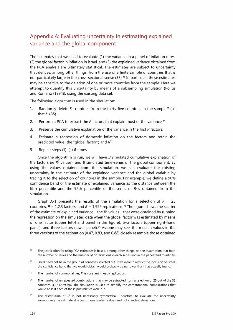
194 BIS Papers No 100
Appendix A: Evaluating uncertainty in estimating explained variance and the global component
The estimates that we used to evaluate (1) the variance in a panel of inflation rates, (2) the global factor in inflation in Israel, and (3) the explained variance obtained from the PCA analysis are ultimately statistical. The estimates are subject to uncertainty that derives, among other things, from the use of a finite sample of countries that is not particularly large in the cross-sectional sense (35).21 In particular, these estimates may be sensitive to the deletion of one or more countries from the sample. Here we attempt to quantify this uncertainty by means of a subsampling simulation (Politis and Romano (1994)), using the existing data set.
The following algorithm is used in the simulation:
1. Randomly delete K countries from the thirty-five countries in the sample22 (sothat K<35).
2. Perform a PCA to extract the P factors that explain most of the variance.23
3. Preserve the cumulative explanation of the variance in the first P factors.
4. Estimate a regression of domestic inflation on the factors and retain thepredicted value (the “global factor”) and R2.
5. Repeat steps (1)–(4) B times.
Once the algorithm is run, we will have B simulated cumulative explanation ofthe factors (ie R2 values), and B simulated time-series of the global component. By using the values obtained from the simulation, we can evaluate the existing uncertainty in the estimate of the explained variance and the global variable by tracing it to the selection of countries in the sample. For example, we define a 90% confidence band of the estimate of explained variance as the distance between the fifth percentile and the 95th percentile of the series of R2’s obtained from the simulation.
Graph A-1 presents the results of the simulation for a selection of K = 25 countries, P = 1,2,3 factors, and B = 1,999 replications.24 The figure shows the scatter of the estimate of explained variance—the R2 values—that were obtained by running the regression on the simulated data when the global factor was estimated by means of one factor (upper left-hand panel in the figure), two factors (upper right-hand panel), and three factors (lower panel).25 As one may see, the median values in the three versions of the estimation (0.47, 0.83, and 0.88) closely resemble those obtained
21 The justification for using PCA estimates is based, among other things, on the assumption that both the number of series and the number of observations in each series and in the panel tend to infinity.
22 Israel need not be in the group of countries selected out. If we were to restrict the inclusion of Israel, the confidence band that we would obtain would probably be narrower than that actually found.
23 The number of commonalities, P, is constant in each replication.
24 The number of unrepeated combinations that may be extracted from a selection of 25 out of the 35 countries is 183,579,396. The simulation is used to simplify the computational complications that would arise if each of these possibilities were run.
25 The distribution of R2 is not necessarily symmetrical. Therefore, to evaluate the uncertainty surrounding the estimate, it is best to use median values and not standard deviations.
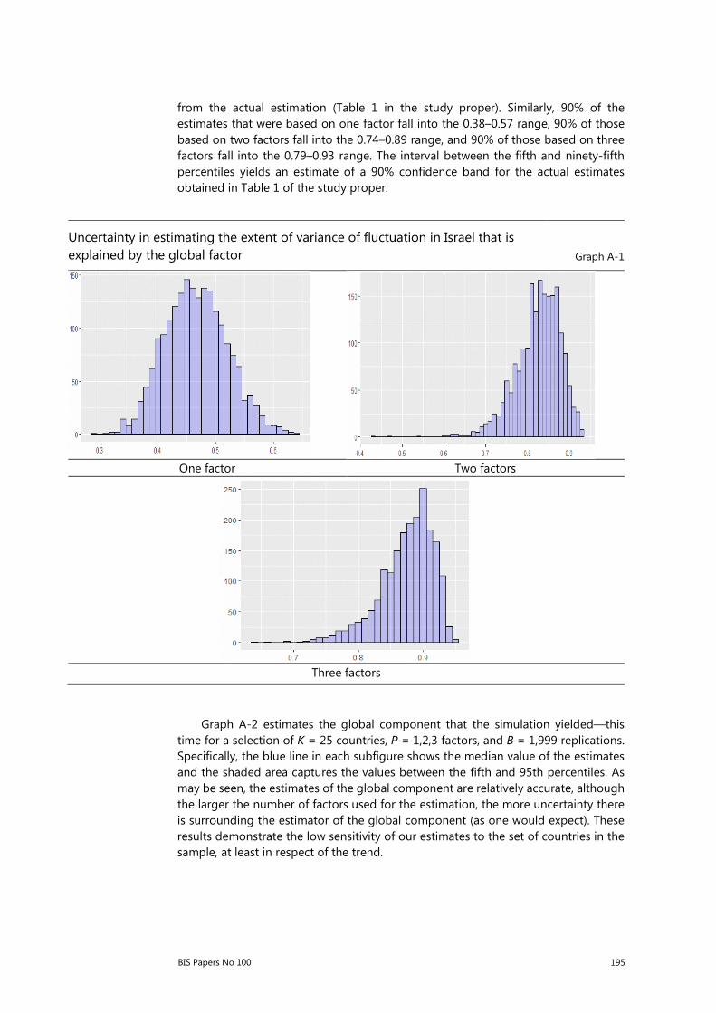
BIS Papers No 100 195
from the actual estimation (Table 1 in the study proper). Similarly, 90% of the estimates that were based on one factor fall into the 0.38–0.57 range, 90% of those based on two factors fall into the 0.74–0.89 range, and 90% of those based on three factors fall into the 0.79–0.93 range. The interval between the fifth and ninety-fifth percentiles yields an estimate of a 90% confidence band for the actual estimates obtained in Table 1 of the study proper.
Uncertainty in estimating the extent of variance of fluctuation in Israel that is explained by the global factor Graph A-1
One factor Two factors
Three factors
Graph A-2 estimates the global component that the simulation yielded—this time for a selection of K = 25 countries, P = 1,2,3 factors, and B = 1,999 replications. Specifically, the blue line in each subfigure shows the median value of the estimates and the shaded area captures the values between the fifth and 95th percentiles. As may be seen, the estimates of the global component are relatively accurate, although the larger the number of factors used for the estimation, the more uncertainty there is surrounding the estimator of the global component (as one would expect). These results demonstrate the low sensitivity of our estimates to the set of countries in the sample, at least in respect of the trend.
196 BIS Papers No 100
Uncertainty in estimating the global component of inflation in Israel Graph A-2
One factor Two factors
Three factors

BIS Papers No 100 197
Appendix B: Additional Sensitivity Tests
B.1 Sensitivity to exclusion of Israel from the panel
Variance in inflation rates explained by factors measured, not including Israel Table B-1
Explained variable Variance explained (𝑅𝑅2) by
1 factor 2 factors 3 factors
Inflation, total 0.44 0.80 0.87
[0.36, 0.51] [0.69, 0.84] [0.79, 0.93]
Inflation, tradable prices 0.56 0.61 0.70
[0.51, 0.61] [0.54, 0.66] [0.59, 0.81]
Inflation, non-tradable prices 0.19 0.71 0.74
[0.13, 0.26] [0.56, 0.82] [0.59, 0.87]
Notes: The table presents the variance in annual inflation—total, tradable, and non-tradable—that is explained by the global factor. The explained variance is defined by an R2 value obtained by running a regression of the relevant inflation rate on an intercept and on the factor/factors. The factors were estimated by means of a panel that does not include Israel’s inflation rate. A 90 percent% confidence band appears in the brackets. (The method of calculation is explained in Appendix A.) The sample used for the calculations is January 2009–March 2017.
Sources: CBS and OECDstat.
B.2 Sensitivity to estimation period
Variance in inflation rates explained by factors in sample beginning in January 2010 Table B-2
Explained variable Variance explained (𝑅𝑅2) by
1 factor 2 factors 3 factors
Inflation, total 0.76 0.85 0.89
[0.71, 0.80] [0.77, 0.93] [0.81, 0.93]
Inflation, tradable prices 0.67 0.84 0.84
[0.62, 0.72] [0.72, 0.91] [0.75, 0.89]
Inflation, non-tradable prices 0.71 0.74 0.83
[0.66, 0.75] [0.73, 0.83] [0.74, 0.87]
Notes: The table presents the variance in annual inflation—total, tradable, and non-tradable—that is explained by the global factor. The explained variance is defined by an R2 value obtained by running a regression of the relevant inflation rate on an intercept and on the factor/factors. The factors were estimated by means of a panel that does not include Israel’s inflation rate. A 90 percent% confidence band appears in the brackets. (The method of calculation is explained in Appendix A.) The sample used for the calculations is January 2010–March 2017.
Sources: CBS and OECDstat.

198 BIS Papers No 100
Variance in inflation rates explained by factors in sample beginning in January 2008 Table B-3
Explained variable Variance explained (𝑅𝑅2) by
1 factor 2 factors 3 factors
Inflation, total 0.61 0.86 0.90
[0.53, 0.67] [0.61, 0.69] [0.84, 0.93]
Inflation, tradable prices 0.64 0.69 0.70
[0.59, 0.67] [0.64, 0.72] [0.66, 0.74]
Inflation, non-tradable prices 0.37 0.72 0.87
[0.31, 0.44] [0.46, 0.88] [0.75, 0.88]
Notes: The table presents the variance in annual inflation—total, tradable, and non-tradable—that is explained by the global factor. The explained variance is defined by an R2 value obtained by running a regression of the relevant inflation rate on an intercept and on the factor/factors. The factors were estimated by means of a panel that does not include Israel’s inflation rate. A 90 percent% confidence band appears in the brackets. (The method of calculation is explained in Appendix A.) The sample used for the calculations is January 2008–March 2017.
Source: CBS and OECDstat.
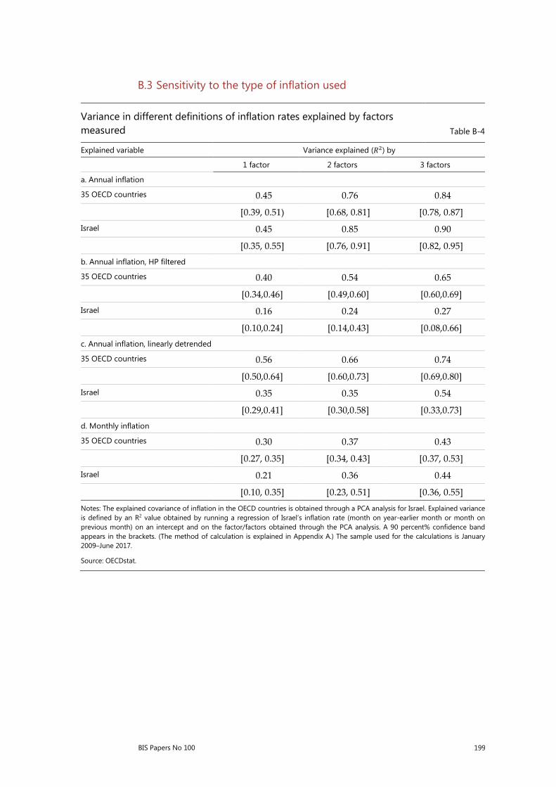
BIS Papers No 100 199
B.3 Sensitivity to the type of inflation used
Variance in different definitions of inflation rates explained by factors measured Table B-4
Explained variable Variance explained (𝑅𝑅2) by
1 factor 2 factors 3 factors
a. Annual inflation
35 OECD countries 0.45 0.76 0.84 [0.39, 0.51) [0.68, 0.81] [0.78, 0.87] Israel 0.45 0.85 0.90
[0.35, 0.55] [0.76, 0.91] [0.82, 0.95] b. Annual inflation, HP filtered
35 OECD countries 0.40 0.54 0.65 [0.34,0.46] [0.49,0.60] [0.60,0.69] Israel 0.16 0.24 0.27
[0.10,0.24] [0.14,0.43] [0.08,0.66] c. Annual inflation, linearly detrended
35 OECD countries 0.56 0.66 0.74 [0.50,0.64] [0.60,0.73] [0.69,0.80] Israel 0.35 0.35 0.54
[0.29,0.41] [0.30,0.58] [0.33,0.73] d. Monthly inflation
35 OECD countries 0.30 0.37 0.43 [0.27, 0.35] [0.34, 0.43] [0.37, 0.53] Israel 0.21 0.36 0.44
[0.10, 0.35] [0.23, 0.51] [0.36, 0.55] Notes: The explained covariance of inflation in the OECD countries is obtained through a PCA analysis for Israel. Explained variance is defined by an R2 value obtained by running a regression of Israel’s inflation rate (month on year-earlier month or month on previous month) on an intercept and on the factor/factors obtained through the PCA analysis. A 90 percent% confidence band appears in the brackets. (The method of calculation is explained in Appendix A.) The sample used for the calculations is January 2009–June 2017.
Source: OECDstat.

200 BIS Papers No 100
B.4 Correlations of the common factors
Correlation among factors and oil prices and USD exchange rate Table B-5
F1 F2 Oil DXY
F1 —
F2 0 —
Oil 0.63 0.01 —
DXY -0.57 0.07 -0.87 —
Notes: The table presents correlation coefficients for the first two common factors (marked by F1, F2), Oil, and DXY. All variables are expressed in terms of annual rates of change (month on year-earlier month). The underlying sample period is January 2009–June 2017.
Source: OECDstat.
B.5 Factor analysis for core, tradable, and non-tradable inflation
Explanatory power of factors for variance in inflation rates, excluding food and energy Table B-6
Explained variable Variance explained (𝑅𝑅2) by
1 factor 2 factors 3 factors
Inflation in OECD countries 0.31 0.47 0.61
[0.27, 0.35] [0.44, 0.53] [0.57, 0.63]
Inflation in Israel 0.76 0.81 0.90
[0.60, 0.85] [0.63, 0.91] [0.76, 0.95]
Notes: The explained covariance of inflation in the OECD countries is obtained through a PCA analysis for Israel. Explained variance is defined by an R2 value obtained by running a regression of Israel’s inflation rate on an intercept and on the factor/factors obtained through the PCA analysis. A 90 percent% confidence band appears in the brackets. (The method of calculation is explained in Appendix A.) The sample used for the calculations is January 2009–June 2017.
Source: OECDstat.

BIS Papers No 100 201
Explanatory power of factors for variance in tradable and non-tradable inflation Table B-7
Explained variable Variance explained (𝑅𝑅2) by
1 factor 2 factors 3 factors
Inflation, total 0.45 0.85 0.90
[0.35, 0.55] [0.76, 0.91] [0.82, 0.95]
Inflation, tradable G&S 0.56 0.62 0.70
[0.50, 0.62] [0.56, 0.68] [0.62, 0.82]
Inflation, non-tradable G&S 0.20 0.75 0.77
[0.14, 0.29] [0.32, 0.87] [0.64, 0.89]
Notes: The table presents the variance in annual inflation—total, tradable, and non-tradable—that is explained by the global component. The explained variance is defined by an R2 value obtained by running a regression of the relevant inflation rate on an intercept and on the factor/factors. A 90 percent% confidence band appears in the brackets. (The method of calculation is explained in Appendix A.) The sample used for the calculations is January 2009–June 2017.
Source: CBS and OECDstat.
Appendix C: Common factor or dominant country?
One possible critique of the use of the factor model and, particularly, the use of PCA for estimation purposes is that the strong correlation observed may have been produced by means of one country or a small number of countries that effectively dictated the pace of all the others. In the extreme case, one bloc of countries (e.g., the United States and Germany) is ostensibly the factor that dictates the inflation rates of all the rest.
To test this hypothesis, we ran for each country separately a regression of the country’s inflation rate on the inflation rates of the other OECD member states and used a statistical method to select relevant variables for the regression, so that “important” variables would be non-zero and “unimportant” ones zeroed. Formally, we estimated the following model for each country:
𝜋𝜋𝑖𝑖𝑖𝑖 = 𝛽𝛽0 +∑ 𝛽𝛽𝑗𝑗𝜋𝜋𝑗𝑗𝑖𝑖𝑘𝑘𝑗𝑗=1 + 𝜀𝜀𝑖𝑖𝑖𝑖 , 𝑘𝑘 ≠ 𝑖𝑖,
where in our case k = 34 is the number of countries (apart from country i) in the sample. To select the relevant variables, we used the LASSO estimator, which sustains the following condition:
�̂�𝛽𝜆𝜆𝐿𝐿𝐿𝐿𝐿𝐿𝐿𝐿𝐿𝐿 = arg max
𝛽𝛽0,𝛽𝛽1,…,𝛽𝛽𝑘𝑘��𝜋𝜋𝑖𝑖𝑖𝑖 − 𝛽𝛽0 + �𝛽𝛽𝑗𝑗𝜋𝜋𝑗𝑗𝑖𝑖
𝑘𝑘
𝑗𝑗=1
�
2
+ 𝜆𝜆��𝛽𝛽𝑗𝑗�𝑘𝑘
𝑗𝑗=1
𝑇𝑇
𝑖𝑖=1

202 BIS Papers No 100
The limitation that appears in this formulation, 𝜆𝜆∑ �𝛽𝛽𝑗𝑗�𝑘𝑘𝑗𝑗=1 , “forces” the model to
zero some of the coefficients.26 When 𝜆𝜆 = 0, ie when the “penalty” for breaching the limit is zero, the LASSO estimates for 𝛽𝛽𝑗𝑗 are identical to ordinary OLS estimates.
The only remaining task in estimating the model is to choose a value for 𝜆𝜆. To do this, we ran the model for values of 𝜆𝜆 between zero and 1 and chose the 𝜆𝜆 that led to the lowest average AIC value (for the full set of countries).27 The value chosen for 𝜆𝜆 stood at 0.0008, at which an average AIC value of 157.9 was obtained. The choice of a value very close to zero as the optimal one (in accordance with the AIC criterion) already indicates that our LASSO estimates will be very close to the OLS estimates; ie one should expect not to obtain too many zeroed estimates.
Figure C-1 presents the results of the estimation. The explained variables (inflation rates parsed by individual countries) appear on the y-axis and the explanatory variables (inflation rates in all countries apart from the explained country) are arrayed on the x-axis. A gray cell in the matrix indicates that the coefficient for that country is non-zero; a blue cell represents a zeroed coefficient. As the figure demonstrates clearly, most coefficients of the countries in all regressions are non-zero, giving evidence that the sparsity assumption is probably a poor fit in our case. Namely, it does not stand to reason that one country or a small number of countries dictates the pace.
26 This contrasts with ridge estimators, for example, which merely compress the coefficients toward zero
without forcing the issue.
27 The AIC value decreases as the sum of the squares of the deviations of the model increases and increases as the number of explanatory values in the regression rises. The optimal AIC value is the lowest.
LASSO coefficient matrix Graph C-1
United StatesUnited KingdomTurkeySwitzerlandSwedenSpainRepublic of KoreaSloveniaSlovakiaPortugalPolandNorwayNew ZealandNetherlandsMexicoLuxembourgLatviaJapanItalyIsraelIrelandIcelandHungaryGreeceGermanyFranceFinlandEstoniaDenmarkCzech RepublicChileCanadaBelgiumAustriaAustralia
Aus
tral
iaA
ustr
iaBe
lgiu
mC
anad
aC
hile
Cze
ch R
epub
licD
enm
ark
Esto
nia
Finl
and
Fran
ceG
erm
any
Gre
ece
Hun
gary
Icel
and
Irel
and
Isra
elIta
lyJa
pan
Latv
iaLu
xem
bour
gM
exic
oN
ethe
rland
sN
ew Z
eala
ndN
orw
ayPo
land
Port
ugal
Repu
blic
of K
orea
Slov
akia
Slov
enia
Spai
nSw
eden
Switz
erla
ndTu
rkey
Uni
ted
Kin
gdom
Uni
ted
Stat
es
Input variables
Resp
onse
var
iabl
e
Coefficient ZeroNonzero
BIS Papers No 100 203
Appendix D: Data
D.1 Inflation in OECD countries
In this study, we used monthly data to determine the annual inflation rate (month on year-earlier month) and monthly data for the period between January 2009 and June 2007. Our source of data was OECD.Stat.28 Data for all countries are monthly except for Australia and New Zealand, for which they are quarterly. To convert the quarterly data into monthly data, linear interpolation was used. Table D-1 presents comparative statistics of the data on the basis of the sample and Figure D-1 graphs the (standardised) data for each country.
28 For the list of OECD member states, see http://www.oecd.org/about/membersandpartners/

204 BIS Papers No 100
Comparative statistics: Annual inflation rates in OECD countries,
January 2009–June 2016 Table D-1
Countries Mean Median Max Min. Std. Dev.
Australia 2.2 2.1 3.5 1 0.7
Austria 1.7 1.7 3.6 -0.3 0.9
Belgium 1.6 1.7 3.8 -1.7 1.3
Canada 1.5 1.4 3.7 -0.9 0.8
Chile 3 3 6.3 -2.3 1.7
Czech Republic 1.4 1.3 3.7 -0.1 1
Denmark 1.3 1 3.1 -0.1 0.9
Estonia 1.9 2 5.7 -2.1 2.3
Finland 1.2 1 4 -1.6 1.3
France 0.9 0.8 2.5 -0.7 0.8
Germany 1.1 1.2 2.4 -0.5 0.8
Greece 0.8 0.6 5.6 -2.9 2.3
Hungary 2.6 2.7 6.6 -1.5 2.3
Iceland 4.3 3.3 18.6 0.8 3.5
Ireland -0.1 0.2 3.1 -6.5 2.1
Israel 1.4 1.5 4.3 -1 1.6
Italy 1.2 1.2 3.4 -0.6 1.2
Japan 0.2 0 3.7 -2.5 1.3
Latvia 1.4 0.7 9.8 -4.2 2.4
Luxembourg 1.5 1.5 3.7 -0.7 1.2
Mexico 3.9 3.7 6.3 2.1 1
Netherlands 1.5 1.4 3.1 -0.2 0.9
New Zealand 1.6 1.5 5.3 0.1 1.2
Norway 2.1 2 4.4 0.1 0.9
Poland 1.7 1.8 4.8 -1.3 2
Portugal 1 0.7 4.2 -1.7 1.5
Slovakia 1.3 1 4.6 -0.9 1.6
Slovenia 1.1 1.3 3.3 -0.9 1.1
South Korea 2 1.6 4.7 0.4 1.1
Spain 1 0.8 3.8 -1.4 1.5
Sweden 0.7 0.5 3.4 -1.9 1.2
Switzerland -0.2 -0.2 1.4 -1.4 0.6
Turkey 7.9 7.9 11.9 4 1.7
United Kingdom 2.2 2.4 5.2 -0.1 1.4
United States 1.4 1.5 3.9 -2.1 1.2
All 1.7 1.5 18.6 -6.5 2.1
Source: OECDstat.

BIS Papers No 100 205
Annual inflation rates, OECD countries Graph D-1
Source: OECDstat.

206 BIS Papers No 100
Appendix E: Additional factor analysis results
Marginal and cumulative contribution of factors to the explanation of inflation in OECD countries Graph E-1
Notes: The figure presents the marginal R^2 values from a regression of the annual inflation rate in each country on a constant and the first two common factors. The length of each bar indicates the total variance explained by the two factors. The sample period used for the estimation is January 2009–June 2017.
TurkeySwitzerlandLuxembourgPolandAustraliaChileJapanNetherlandsNorwayNew ZealandCzech RepublicSwedenGreeceCanadaUnited StatesLatviaRepublic of KoreaBelgiumIcelandSloveniaEstoniaHungaryFinlandSlovakiaItalyIsraelSpainGermanyMexicoDenmarkUnited KingdomPortugalAustriaIrelandFrance
0.00 0.25 0.50 0.75 1.00Proportion of variance explained R2
Cou
ntry
1st Factor
2nd Factor

BIS Papers No 100 207
Sensitivity of individual inflation rates to the common factors Graph E-2

208 BIS Papers No 100
Annual inflation in selected countries and the contribution of the global component, obtained by a latitudinal approach Graph E-3
(a) United States (b) Germany
(c) Australia (d) Japan

BIS Papers No 100 209
Foreign workers in the Korean labour market: current status and policy issues
Seung-Cheol Jeon1
Abstract
The number of foreign workers in Korea is growing rapidly, increasing from 1.1 million in 2012 to 1.4 million in 2016. As a result, the impact of foreign workers on the labour market and Korean society is expected to increase.
As industrialisation and income levels advanced from the late 1980s, a shortage of low-skilled workers developed. From the early 1990s, the industrial trainee system encouraged an influx of foreign workers. Currently, quotas for foreign workers are in place to ensure their orderly entry and management.
The inflow of foreign workers is seen to have had a generally positive effect on the Korean economy, contributing to domestic economic growth by increasing labour input in industries that are less favoured by domestic workers, and easing the trend towards workforce ageing in the Korean labour market. But, as most foreign workers are engaged in low-skilled, low-wage occupations, the inflow has tended to exacerbate labour market polarisation and to delay the restructuring of marginal companies.
Keywords: Foreign workers, Korean labour market, foreign workforce policy.
JEL classification: F16, J61, J68.
1 Deputy Governor, Bank of Korea.

210 BIS Papers No 100
I. Background
The foreign working-age population2 in Korea is growing rapidly, increasing from 1.114 million in 2012 to 1.425 million in 2016. As of 2016, the foreign labour force numbered 1.005 million persons, of whom 962,000 persons were in employment and 43,000 persons unemployed. As the pace of influx of foreign employees continues to outstrip growth in the total number of the employed, the share of the foreign workers in the overall domestic labour market has been rapidly increasing.
As a result, the impact of foreign workers on the labour market and Korean society are expected to increase. Against this backdrop, this paper analyses Korea’s foreign workforce and examines the related policy implications.
Ⅱ. Foreign workers in the Korean labour market
1. Foreign workforce policy in Korea
As industrialisation and income levels advanced from the late 1980s, a shortage of low-skilled workers developed. From the early 1990s, there was an influx of foreign workers, due mainly to the industrial trainee system.3 However, poor management of the system led to problems such as corrupt brokers and workers fleeing their workplaces. Later, with improvements such as the introduction of a foreign employment permit system in 2003, regulations on the employment of foreign
2 Foreign population aged 15 or over with long-term visa status.
3 At the initial stage, companies with overseas local branches imported foreign workers by sending them to domestic sites for technical training (for six months). Later, the influx of foreign workers increased as companies without overseas local branches were allowed to hire trainees.
Graph 1
Foreign working-age population Ratio of foreign workers1
Source: Statistics Korea. 1 Foreign employed/total domestic employed and foreign labour force/total domestic labour force
Source: Statistics Korea.

BIS Papers No 100 211
workers were eased and employment protections for foreign workers were strengthened. As a result, the number of such workers increased rapidly.
Under the current employment permit system, foreigners with long-term visas who are eligible to work in Korea can be classified into two main categories: non-professional and professional. Non-professional workers hold mostly non-professional employment (E-9), working visit 4 (H-2) or compatriot 5 (F-4) visas. Foreign workers with working visit and compatriot visas can search for jobs autonomously after arriving in Korea, and they can be employed in a wider range of industries than can those with non-professional employment visas. The number of professional workers6 is not large, and of them language instructors account for the largest share.
Currently, quotas7 for foreign workers are in place to ensure their orderly entry and management. In the case of the general employment permit system (E-9), a quota8 of about 50,000 new general foreign workers is assigned by industry every year. In the case of foreign workers with working visit (H-2) visas, these stood at 303,000 persons, with the total number being limited. However, since requirements for receiving these visas are relatively strict, about 270,000 compatriots are reported to have such visas as of the end of 2016.
Foreign population with long-term visa status1 Graph 2
1 As of September 2017, compatriots with foreign nationality have been excluded.
Source: Ministry of Justice.
4 Working visit visas are for compatriots aged 25 or older who reside in China or areas of the former
Soviet Union. They may stay in Korea for up to three years.
5 Those with compatriot visas have obtained foreign nationality, and either they or one of their parents (or one of their grandparents) have Korean nationality. They may stay in Korea for two years.
6 Journalism (D-5), religion (D-6), supervisors (D-7), corporate investors (D-8), international trade (D-9), professors (E-1), foreign language instructors (E-2), research (E-3), technology transfer (E-4), professional employees, including lawyers (E-5), designated activities (E-7) etc.
7 The Foreign Workforce Policy Committee of the Prime Minister’s Office decides the number of foreign workers who will be permitted entry and the industries in which foreign workers are allowed to work.
8 In 2017, the total quota for new general foreign workers was 56,000.

212 BIS Papers No 100
As for other foreigners with long-term visas, a large number are foreign students (D-2, D-4-1) and married immigrants and permanent residents (F-2-1, F-6, F-5), and their number has recently been on the rise.
At the early stage of labour market opening, the Korean government allowed foreign workers to remain employed only temporarily to help solve the nation’s labour shortage, while restricting them from settling in Korea permanently.9 Since the 1980s, when the trainee system was introduced to respond to increased demand for low-wage foreign labour in line with rapid economic growth, the aim of Korea’s foreign workforce policy has been to supplement the domestic labour market.
Taking into account domestic labour market conditions, the current employment permit system still restricts the employment of foreigners by means of regulations concerning the location and period of employment. To protect domestic workers, foreign workers are allowed to remain employed for a maximum of five years, and the number of foreign workers introduced is adjusted annually depending on domestic labour market conditions. Furthermore, there are many regulations regarding both employers and foreign workers ― employers have to make efforts to hire domestic workers before hiring foreign workers, 10 and foreign workers face restrictions on changing their workplace during the period of employment.
9 Article 1 of Chapter 1 of the Act on the Employment etc of Foreign Workers stipulates its purpose as
contributing to the smooth supply of and demand for human resources and the balanced development of the national economy through the systematic introduction and management of foreign workers.
10 Employers must post job openings for domestic workers at employment security agencies such as manpower banks, and only if they then fail to hire domestic workers are they allowed to apply for permits to employ foreign workers.
Graph 3
Foreign students1
Married immigrants1 and permanent residents2
1) D-2 and D-4-1
Source: Statistics Korea.
1 F-2-1 and F-6 2 F-5
Source: Statistics Korea.
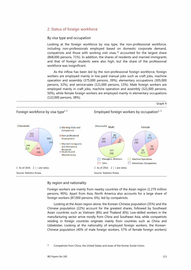
BIS Papers No 100 213
2. Status of foreign workforce
By visa type and occupation
Looking at the foreign workforce by visa type, the non-professional workforce, including non-professionals employed based on domestic corporate demand, compatriots and those with working visit visas, 11 accounted for the largest share (868,000 persons, 71%). In addition, the shares of residents and married immigrants and that of foreign students were also high, but the share of the professional workforce was insignificant.
As the inflow has been led by the non-professional foreign workforce, foreign workers are employed mainly in low-paid manual jobs such as craft jobs, machine operation and assembly (375,000 persons, 39%), elementary occupations (305,000 persons, 32%), and service·sales (121,000 persons, 13%). Male foreign workers are employed mainly in craft jobs, machine operation and assembly (321,000 persons, 50%), while female foreign workers are employed mainly in elementary occupations (122,000 persons, 38%).
Graph 4
Foreign workforce by visa type1, 2 Employed foreign workers by occupation1, 2
1 As of 2016 2 ( ) are ratios
Source: Statistics Korea.
1 As of 2016 2 ( ) are ratios
Source: Statistics Korea.
By region and nationality
Foreign workers are mainly from nearby countries of the Asian region (1.279 million persons, 90%). Apart from Asia, North America also accounts for a large share of foreign workers (87,000 persons, 6%), led by compatriots.
Looking at the Asian region alone, the Korean-Chinese population (35%) and the Chinese population (22%) account for the greatest shares, followed by Southeast Asian countries such as Vietnam (8%) and Thailand (6%). Low-skilled workers in the manufacturing sector arrive mostly from China and Southeast Asia, while compatriots residing in foreign countries originate mainly from countries such as China and Uzbekistan. Looking at the nationality of employed foreign workers, the Korean-Chinese population (40% of male foreign workers, 57% of female foreign workers)
11 Compatriots from China, the United States and areas of the former Soviet Union.

214 BIS Papers No 100
accounts for the majority, while the shares of Vietnam (7%) and Indonesia (6%) are high for male workers, and those of the non-Korean-Chinese population (10%) and Vietnam (7%) are high for female workers.
By industry
By industry, the manufacturing industry (45%) accounts for the largest share of the total foreign workforce, followed by wholesale and retail and restaurants and hotels (20%), business, personal, public services and others (19%),12 and construction (9%). The largest proportion of male foreign workers is employed in the manufacturing industry (55%), while the biggest share of female foreign workers is employed in the wholesale and retail, and restaurants and hotels industries (40%).
Looking at the share of foreign workers in the total number of persons employed, foreign workers occupy much larger shares of the manufacturing sector and the business, personal, public services and others sectors that include workers dispatched by temporary work agencies.
12 A majority of foreign workers in the business, personal and public services and other services
industries are engaged in construction as workers dispatched by temporary work agencies.
Graph 5
Foreign workforce by region1, 2
Asian foreign population1 by country of origin 2
1 As of 2016 2 ( ) are ratios
Source: Statistics Korea.
1 Total Foreign Population 2 As of 2016
Source: Ministry of Justice.

BIS Papers No 100 215
Graph 6
Employed foreign workers by industry1, 2 Ratio of foreign workers to total workers
by industry1
1 As of 2016 2 ( ) are ratios
Source: Statistics Korea.
1 As of 2016
Source: Statistics Korea.
Meanwhile, as the number of foreign workers rises, their international remittances are also increasing rapidly. Looking at the annual value of international remittances13 by foreign workers who have been employed for less than a year and on whom statistics are available,14 the value has grown significantly, from around UD 600 million during the financial crisis (in 2008 and 2009) to USD 1.374 billion as of 2016.
Wages and salaries paid to non-resident workers1 Graph 7
1 Non-resident workers are foreign workers who have been working for less than a year.
Source: Bank of Korea.
By wage level
As a majority of foreign workers are engaged in low-income elementary occupations, nearly half of them (49%) occupy the USD 860–1,700 bracket in terms of monthly average earnings. Due to the gender differences in major occupations, male workers are concentrated in the bracket of USD 1,700–2,600 (46%), while a majority of female
13 Wages and salaries paid to non-resident workers recorded on the balance of payments.
14 38% of total foreign workers as of 2016.

216 BIS Papers No 100
workers belong to the bracket of USD 860–1,700 (64%). Compared with 2015, however, the overall wage level has increased.
Graph 8
Employed foreign workers by monthly average earnings1
Change of the distribution of monthly average earnings of employed foreign workers1
1 As of 2016
Source: Statistics Korea.
1 2016 Distribution - 2015 Distribution
Source: Statistics Korea.
Ⅲ. Effects of the inflow of foreign workers
The inflow of foreign workers is seen to have had a generally positive impact on the Korean economy, contributing to domestic economic growth by increasing labour input in industries that are less favoured by domestic workers,15 and easing the trend towards the ageing of the workforce in the Korean labour market. As most foreign workers are engaged in low-wage occupations requiring a lower level of skills, however, the inflow has tended to exacerbate labour market polarisation and to delay the restructuring of marginal companies.
1. Positive effects
The inflow of foreign workers has helped ease the labour shortage in sectors less favoured by domestic workers due to poor working conditions, such as long working hours and low wages. This is because foreign workers are employed in manufacturing and low-wage sectors that require long working hours and shift-work.
15 According to the IOM Migration Research & Training Centre (2011), the GDP enhancement effect of immigrant workers was estimated at 1.08% as of 2008.

BIS Papers No 100 217
Graph 9
Employed workers by monthly average working hours1
Employed workers by monthly average earnings1
1 As of 2016
Source: Statistics Korea, Ministry of Employment and Labour
1 As of 2016
Source: Statistics Korea, Ministry of Employment and Labour
Specifically, foreign workers are helping to solve the labour shortage in SMEs. Owing to the employment permit system that restricts the size of eligible workplaces, most foreign workers are engaged by small-sized employers. As SMEs have more difficulty than large corporations in hiring people, and this gap is widening, their demand for foreign workers is growing steadily.
Graph 10
Employed workers by company size1 Labour force situation (business survey index) by company size1
1 As of 2016
Sources: Statistics Korea, Ministry of Employment and Labour.
1 Smaller value implies shortage of labour supply 2 Monthly Average, Year 2017 is monthly average from Jan. to Oct.
Source: Bank of Korea.
Foreign workers are also helping to slow the ageing of the workforce in line with that of the population. As the Korean population gets older, workforce ageing is advancing rapidly. But a substantial number of foreign workers are young and prime-age workers, who thus help to slow the ageing trend in the Korean labour market. This will not be a fundamental solution to workforce ageing, however, given that foreign workers will also age in the long run (Choi (2010)).

218 BIS Papers No 100
Graph 11
Population and population projection Employed workers by age1
Source: Statistics Korea. 1 As of 2016.
Source: Statistics Korea.
2. Negative effects
Foreign workforce inflows have exacerbated the polarisation of the labour market. Since industries that need highly educated talent hire primarily Korean workers, while foreign workers are engaged in SMEs or in industries with low wages and low productivity, their inflows have been one of the factors expanding the wage gap in some industries. In manufacturing, for example, the wage gap between SMEs and large companies has widened as a consequence of the increasing number of foreign workers employed in businesses with less than 300 regular workers. 16 In the food and accommodation sector, which has a high share of foreign workers, the low wage structure has intensified.
16 Under the Employment Permit System (including the general and special systems), only manufacturing businesses with fewer than 300 regular workers or KRW 8 billion or less in capital are allowed to employ foreign workers.

BIS Papers No 100 219
Graph 12
Hourly earnings (manufacturing sector)1, 2 Hourly earnings1
1 Total earnings/total hours 2 Small & mid: 5–299 employees, Large: 300+ employees
Source: Ministry of Employment and Labour.
1 Total earnings/total hours
Source: Ministry of Employment and Labour.
On the other hand, the number of foreign professionals has remained little changed17 at around 50,000 persons; most foreign professionals are invited as foreign language instructors or cooks, and the share of highly talented foreign professionals, such as professors and researchers, is only 12%.
Graph 13
Employed workers1 by education2 Professional foreign employment by visa type1, 2
1 Foreign Workforce for foreigners 2 As of 2016
Source: Statistics Korea.
1 C-4 (Temporary Employment) and E1~7 2 Designated Activities are mostly Cook and Chef
Source: Ministry of Justice.
The flow of foreign workers mainly into low-income and low-skilled sectors also tends to delay the restructuring of marginal enterprises, since these companies are able to survive based on their cheap foreign labour.
17 48,000 persons in 2012 and 46,000 persons in 2016, based on workers with E-1 to E-7 visas.
220 BIS Papers No 100
Ⅳ. Conclusions and policy implications
The relationship between foreign and Korean workers in the Korean labour market is considered a supplementary one. Given the decline in the working-age population, foreign workers, many of whom are members of the core age group, are employed in sectors with an insufficient supply of domestic workers. In this way, foreign workers help to prevent offshoring in the manufacturing sector, hence expanding employment18 and raising Korea’s GDP. On the other hand, given that foreign workers are engaged mainly in low-wage and low-skilled sectors, there are negative results as well, such as more acute polarisation of the labour market and the delayed restructuring of marginal enterprises. Going forward, structural reforms to ease the labour market dualism, and policies to promote social consolidation between foreign and domestic workers are necessary.
Meanwhile, according to the five-year basic plan for immigration policy,19 which serves as the basis for all policies related to foreigners, the Korean government will continue to focus on low-wage, non-professional migrant workers to ease labour shortages in non-preferred industries.
18 An empirical study (Kang (2017)) found that an increase in the number of foreign workers leads to a rise in the employment of domestic workers, thanks to expanded production.
19 Starting from 2008, the Ministry of Justice has developed a basic plan for immigration policy every five years, in consultation with related ministries. Currently, research on the development of the third basic plan for immigration policy has been completed (November 2016, IOM MRTC, worker paper requested by the Ministry of Justice).

BIS Papers No 100 221
References
Choi, H Y (2013): “Legal issues related to long-term hiring of foreign workforce”, Korean Journal of Labour Law, vol 48, pp 419–55.
Choi, K S (2010): “Mid to long-term effect of migration and foreign workforce inflow on domestic labour market”, KDI Working Papers, Korea Development Institute.
Kang, D G (2017): “Economic activity and effects of immigrants”, Policy Report, Migration Research and Training Center, February.
Kang, H W (2006): “Formation of multicultural society and integration policy”, Journal of National Policy Research, vol 20, no 2, pp 5–34.
Migration Research and Training Center (2016): “Research on the Third Foreign Population Policy”, November.
Business Survey, Bank of Korea.
Foreign Workforce Survey, Statistics Korea.
Immigration Statistics, Ministry of Justice.
Labor Force Survey, Statistics Korea.
National Accounts, Bank of Korea.
Survey on Employment by Occupational Type, Ministry of Employment and Labor.

222 BIS Papers No 100

BIS Papers No 100 223
Globalisation and deglobalisation
Central Bank of Malaysia
Abstract
Malaysia’s integration into global value chains has played a crucial role in the recent development of the economy, helping to promote its diversification into higher value added and services-based manufacturing. Globalisation has also enabled technological advances and higher investment. This has led to faster income growth, particularly for capital owners and highly skilled workers. However, Malaysia is also now faced with new issues, such as a heavier reliance on foreign workers and heightened vulnerability from global developments. In particular, Malaysia also faces challenges posed by highly volatile capital flows. Moving forward, the global economy will inevitably become more interconnected. The policy imperative is to develop a labour force that is able to respond quickly to changing global demands, strengthen economic fundamentals to protect economic resilience and continuously implement structural reforms to future-proof the economy.
Keywords: Globalisation, regional integration, global value chain, trade openness, technological advancement, flexible labour market, international policy cooperation, financial integration, trade protectionism.
JEL classification: F60, F62, F63, F66 and F68.

224 BIS Papers No 100
Determinants of international trade and population flows
Since the Great Financial Crisis (GFC), global trade has grown more slowly than the global economy itself. This is due to both cyclical and structural factors. Firstly, persistent economic weakness, particularly subdued investment in the advanced economies, has dampened global trade. Structural factors are also at play, in particular, the diminishing impact of major catalytic factors that were important drivers of the high global trade growth in the 1990s and early 2000s. These include the proliferation of global value chains (GVC), breakthroughs of major trade liberalisations such as the formation of the European Union (EU) and World Trade Organisation (WTO) and the accession of PR China into WTO in 2001. The future of global trade will depend, among other things, on structural shifts such as China’s economic transition towards a more consumption-based growth, the rising middle income population in the emerging market economies (EMEs), and new and revised multilateral trade agreements.
In Malaysia, exports grew at a slower pace after the GFC (2011–16: 3.6% compared with 11% in 2003–08). However, more recently, exports have grown at the fastest pace since 2004 (Jan–Sep 2017: 21.3%; 2004: 21.0%). Several factors explain this improvement. First, structural reforms have helped to promote greater diversification in the composition of export products, which has enabled Malaysia to benefit from enlarged intra-regional trade. Second, the diversification into the electrical and electronics (E&E) segment and Malaysia’s participation in GVCs have enabled the economy to benefit from the global technology upcycle. Malaysia is the seventh largest global semiconductor exporter, with semiconductor exports totalling USD 35 billion in 2016. Third, the pickup in consumer spending and investment activity in the advanced economies (eg the United States and EU) along with faster expansion in the other EMEs have provided further impetus to Malaysia’s exports.
Malaysia’s integration into GVCs has been facilitated by its openness to trade, attractive investment environment and strong macroeconomic fundamentals (Malaysia’s trade-to-GDP ratio in 2016 was 128% compared with a world average of 88.5%). This has reduced the sensitivity of the exchange rate on exports. External demand remains the most important driver of exports. There are, however, risks. Disruptions along the value chain can affect production and trade by all companies along the value chain. For example, in 2011, the twin disasters of the Tohoku earthquake and floods in Thailand impacted the global electronics production network. Foreign suppliers could not immediately take over the strategic role of some Japanese and Thai suppliers. This resulted in some production disruption in Malaysia’s electronics industry during the period (average growth for electronics IPI in March – May 2011: –16.3%; November 2011: –0.4%).
Research has shown that technological advances have a positive impact on trade and economic growth in general through the introduction of new and improved products, opening of new markets and process innovation.1 In the case of Malaysia, greater technological innovation and its dispersion across borders have helped to
1 L Márquez-Ramos and I Martínez-Zarzoso, “The effect of technological innovation on international
trade: a nonlinear approach”, Economics Discussion Papers, no 2009-24, Kiel Institute for the World Economy, 2009.
BIS Papers No 100 225
advance its overall economic complexity,2 which increased from 0.70 in 2010 to 0.82 in 2016. This has also led to a rapid shift in Malaysia’s export product mix. Within specific E&E products, for example, integrated circuits (which have a higher product complexity of 2.56) have increased their share of Malaysia’s total exports from 9.9% in 2010 to 14% in 2016. Correspondingly, Malaysia's exports of computers (with a lower complexity of 1.94) have declined from 4.8% of total exports in 2010 to 4.2% in 2016. In the services sector, new technology has broadened market reach and allow for quicker and more efficient trade facilitation via e-commerce and the digitisation of cross-border activity. Malaysia recently launched a Digital Free Trade Zone, which aims to connect the small and medium enterprises (SMEs) with electronic marketplaces, government agencies and cross-border logistics and payment providers. Advances in information and communications technology (ICT) also promote efficient movement of goods and people through greater use of online applications (eg e-Visa) and marketing tools (eg social media), with a positive impact on trade and tourism. Technological advances may also pose a risk to employment, due to structural changes and increased automation. The challenge is to develop a labour force that can respond quickly to changing industry needs.
Regional and global arrangements have played a key role in facilitating trade and attracting foreign direct investment (FDI). As a result of strengthened regional production, Malaysia is increasingly positioned as a producer and assembler of the intermediate parts and components of manufactured goods, before they are exported for further processing or final consumption. The share of exports to East Asia and the rest of the world3 has risen from 45.3% in 2001 to 60.2% in 2016. Increased financial integration, particularly in the form of FDI, has contributed to Malaysia’s current trade strength by enabling the country to respond quickly to any increase in global demand. However, the increased role of financial centres and the complexity of corporate structures at large multinational companies (MNCs) make it more challenging for policymakers to separate long-term industrial investments from the investment positions of fund vehicles. Investment via international offshore financial centres (IOFCs) is a common international practice for businesses and companies: investable funds are pooled in IOFCs before being redirected to economic sectors in various locations. For example, the share of Malaysia’s direct investment abroad (DIA) to IOFCs amounted to 24% of total DIA (2016), which is comparable with other regional economies (eg Thailand: 22% in 2016; Singapore: 15.2% in 2015; Hong Kong SAR: 47% in 2015).4
2 Economic complexity captures the diversity and ubiquity of a country’s export of goods. It is
measured as a standard deviation from the world average. A country can improve its ECI position by producing and exporting more complex and diverse products. This methodology was developed by Ricardo Hausmann et al at the Harvard’s Center for International Development. For a more detailed account, please refer to Hausmann, R., et al. (2013), The Atlas of Economic Complexity: Mapping Paths to Prosperity, 2nd ed., Cambridge: MIT Press
3 Other than regional countries, EU member states and advanced economies.
4 Depending on the availability of published data granularity, IOFCs for Malaysia and Singapore include the Cayman Islands, the Isle of Man, Mauritius, the British Virgin Islands and Bermuda; Thailand includes the Cayman Islands, the Isle of Man, Mauritius and the British Virgin Islands; Hong Kong SAR includes the Cayman Islands, the British Virgin Islands and Bermuda. Data is sourced from national authorities.

226 BIS Papers No 100
Macroeconomic and distributional effects of globalisation
Malaysia’s natural resources were once a key determinant of its trade performance. However, the country has sought to expand export capacity through greater emphasis on manufactured exports and export-oriented investment. This has been achieved through industrial policies such as the Industrial Master Plans, the Promotion of Investments Act (PIA 1986) and the liberalisation of trade barriers and regulations. Partnerships with foreign investors have also helped to diversify Malaysia’s exports.
Consequently, over the years, the economy has steadily evolved, diversifying away from labour-intensive upstream activities towards higher value added and services-based manufacturing activities. As a result, the share of the services sector in the economy has increased, rising from 51.2% in 1990–2000 to 52.9% in 2010–16, while the manufacturing sector has remained as the second largest contributor to the economy (1990–2000: 27.6%; 2010–16: 23.2%). The manufacturing sector in particular, has seen a greater focus on export-oriented industries, such as E&E, and resource-based industries. Industries serving the export markets have developed better capacity and efficiency over the years, with greater linkages with other countries in the region. Industries that relied on low cost and low value added business models were gradually phased out, with some relocating to other countries.
In terms of income, capital owners and highly skilled workers stand to gain the most from globalisation. Capital owners are able to more effectively build and scale operations to take advantage of larger markets. Nonetheless, globalisation has accelerated the inflow of foreign direct investment (FDI), which has provided crucial job opportunities, greater market access and higher wages. On average, foreign MNCs pay 40% higher wages than local firms do.5 However, a challenge remains in ensuring a steady supply of industry-ready graduates with relevant skills. At the same time, building local capacity to support foreign MNCs is imperative to manage substantial leakage arising from large imports of goods and services, such as machinery and equipment and intermediate inputs.
While greater trade activity has generally benefited the economy with the development of new manufacturing facilities, Malaysia is also now faced with the issue of efficient management of low-skilled foreign workers. Today, they account for 12.1% of Malaysia’s documented workforce. This impedes the country’s ability to move up the value chain as it discourages firms from automating and adopting technology that will boost productivity. Reliance on foreign workers in Malaysia, particularly in the more labour-intensive sectors of the economy, has led to large remittance outflows. Outward workers’ remittances almost doubled from MYR 17 billion in 2008 to MYR 30 billion in 2016 (2.4% of GDP).
Malaysia’s inflation dynamics have also been affected as a result of globalisation, through changes in both pricing power and wage-setting behaviour. Increasing global integration has resulted in stronger competition, thus limiting domestic firms’ ability to change prices. In addition, greater labour mobility has expanded the pool of available labour for domestic employment, putting downward pressure on labour costs. Together, these factors have contributed to the lower headline inflation
5 OECD (2008) “Do Multinationals Promote Better Pay and Working Conditions?” OECD Employment
Outlook, Paris

BIS Papers No 100 227
experienced since 2000, compared with the levels seen during the 1990s, when inflation was much higher due to rapid economic expansion alongside high employment.
Past efforts towards advancing globalisation have helped economies such as Malaysia’s to diversify their sources of growth. Yet tighter integration leads to greater synchronisation with global economic cycles. Inevitably, developments in the advanced economies have a bearing on Malaysia’s economic performance. To mitigate external shocks and safeguard the domestic economy, it is vital that trade and financial integration be accompanied with more thoroughgoing industrial reforms, a more resilient banking system, stronger capital buffers, deeper financial markets and comprehensive prudential frameworks.
Key policy issues
The optimal degree of openness depends on a country’s economic structure and stage of development. Malaysia has been a consistent proponent of international trade and has benefited through a gradual and phased liberalisation. Recognising the growth potential in the services sector, the government liberalised 46 services subsectors between 2009 and 2012, including telecommunications, healthcare, education and tourism services. Malaysia has also taken steps to raise the capacity and competitiveness of domestic firms via initiatives such as the Services Sector Blueprint and the Logistics and Trade Facilitation Master Plan.
Thus far, Malaysia has signed and implemented six bilateral free trade agreements (FTAs) and six regional FTAs. For instance, under the ASEAN Free Trade Area (AFTA), starting in January 2010, Malaysia with five other ASEAN Member States (Brunei, Indonesia, the Philippines, Singapore and Thailand) became a free trade area for trade in goods. Of significance, the AFTA is conducted in a gradual and phased manner to allow each country to adapt to the trade liberalisation effort. In addition, several categories have also been created (eg the Temporary Exclusion List, Sensitive List and General Exception List) to safeguard the interests of individual countries. The effect of AFTA is reflected in the share of exports to ASEAN in Malaysia’s total exports, which rose from 25.4% in 2010 to 29.4% in 2016.
Increased financial integration amid uncertainties surrounding growth and policy normalisation has also resulted in volatile capital flows. For Malaysia, the orderly intermediation of capital flows is supported by measures to develop domestic capital markets, build resilience in the banking system and enhance external buffers. At the same time, prudential requirements have been set to safeguard the domestic economy from systemic risks arising from excessive foreign exchange liabilities. The negative impact from potential outflows is mitigated by the more balanced profile of foreign holders of government bonds and the stabilising support of domestic institutional investors. As at 3Q 2017, most foreign holders of government bonds were long-term strategic investors, such as asset managers, central banks and governments, as well as pension funds, which account for approximately 82.6% of total foreign investors and result in a more stable foreign participation in the ringgit asset markets. In times of outflows, the smoothing effect of mature domestic institutional players continues to enable an orderly intermediation of funds in the capital markets. Malaysia’s two main pension funds (EPF and KWAP) had a total of
228 BIS Papers No 100
MYR 855 billion of assets under management in 2016, equivalent to 136% of total non-resident holdings in the domestic debt and equity markets.
As an open emerging market economy, in terms of the real and financial sectors, Malaysia is exposed to the vagaries of global economic and financial conditions. As such, an accommodative monetary policy and flexible exchange rate are an important first line of defence, given the limited fiscal policy space. Increased integration with the world has led to challenges in the conduct of monetary policy. For example, financial openness in an environment of rapid movements in global financial flows implies that monetary policy autonomy can only be maintained with the support of a floating exchange rate regime and a high level of reserves. In this way, there is policy scope for both independent monetary policy and managing capital flows, with the impact of capital flows spread between the exchange rate and the foreign exchange reserves. Additionally, monetary policy should only respond to movements and shocks if these events are deemed to materially shift the balance of risks to the outlook for domestic growth and inflation.
The calls for trade protectionism in the advanced economies today threaten to unravel the gains from globalisation. As an open economy, the upsurge in protectionism and insular policies pose a risk to Malaysia. While Malaysia’s diversified export market6 and product mix provide a buffer against these global uncertainties, it is also important for policymakers to remain committed to the integration agenda.
International policy cooperation plays a key role in accelerating greater economic growth, prosperity and wealth. EMEs, particularly in the ASEAN region, have the bargaining power to shape the global trading and financial architecture given the favourable position and demographics of ASEAN countries. ASEAN is home to more than 600 million people and, if considered as a single entity, would represent the sixth largest economy in the world with a combined GDP of USD 2.5 trillion (in 2015). ASEAN is also a major player in the global trading system, with total trade standing at USD 2.3 trillion (in 2015), accounting for the fourth-largest share of total global trade. According to the OECD (2015), the region will sustain an average annual growth of an estimated 5.6% over the next four years and is expected to be the fourth largest trading bloc by 2050. Moreover, in shaping regional financial arrangements, the ASEAN nations together with Japan, Korea and China have achieved significant milestones. These include the enhancement of the regional financial safety net through the Chiang Mai Initiative Multilaterisation (CMIM) as a source of short-term liquidity support to maintain financial stability in the region.
Regional integration complements global integration in increasing global trade and investment by allowing countries to engage in negotiations as blocs rather than as individual countries. For example, the ASEAN Banking Integration Framework (ABIF) complements existing global financial integration frameworks. ASEAN is also involved in integrating itself in the global value chain through free trade agreements such as the Regional Comprehensive and Economic Partnership (RCEP).
Domestic policies can also promote a more globalised economy while protecting the interests of the nation and its people. Malaysia has put in place several measures in this regard, particularly to develop a more flexible labour market to avoid pockets of unemployment and facilitate a more productive use of resources. For example, the
6 Malaysia’s export market is now more diversified, with rising exposure to the regional economies in
the past decade (exports to regional economies in 2006: 44.4%; 2016: 52.3%). Malaysia’s exposure to the United States in terms of export share fell to 10.2% in 2016, from 18.8% in 2006.
BIS Papers No 100 229
government established the 1Malaysia Outplacement Centre (1MOC) in 2016 to help retrenched workers find new jobs. Thus far, the centre has successfully placed 2,400 workers. The recent introduction of the Employment Insurance Scheme (EIS), which offers temporary financial assistance to retrenched workers, also provides for a more comprehensive safety net for employees.
Moving forward
Future technological advances will lead to a more globalised and interconnected world. This will create both opportunities and challenges. As such, it is important for nations to embark on structural reforms to future-proof their economies and people, particularly during the upward phase of the economic cycle. For Malaysia, efforts are ongoing to shift into higher value added industries, as well as to improve soft and hard infrastructure. There is also an urgent need to improve the quality and flexibility of the labour market. This can be done through increasing the platforms for workers to re-skill and upskill, promoting more tech-based courses in universities and inculcating life-long learning practices. It must also be acknowledged that not all segments of society will benefit. Thus, mitigating steps must be put in place to make globalisation safer, to avoid a backlash and unrest.

230 BIS Papers No 100

BIS Papers No 100 231
Globalisation and consumption risk-sharing in emerging market economies
Manuel Ramos-Francia and Santiago García-Verdú, Bank of Mexico1
Abstract
Our aim is to explore how globalisation has affected consumption risk-sharing in emerging market economies. To that end, we implement a consumption risk-sharing test, using the Barro-Ursua Macroeconomic data set. Its span lets us explore historic episodes in which globalisation has markedly changed. We account for risk aversion heterogeneity by using the economies’ estimates of their relative risk aversion coefficients, and for subjective discount factor heterogeneity by estimating panel regressions with fixed effects. Specifically, we explore risk-sharing in emerging market and advanced economies as two groups, and by geographic regions. In most cases, we reject full insurance. However, advanced economies seem to have achieved full insurance in more recent periods. At a regional level, Europe and Asia appear to have attained such a result as well.
Keywords: Risk-sharing, consumption risk-sharing, globalisation.
JEL classification: E21, F6.
Introduction
“The inhabitant of London could order by telephone, sipping his morning tea in bed, the various products of the whole earth, in such quantity as he might see fit, and reasonably expect their early delivery upon his doorstep; he could at the same moment and by the same means adventure his wealth in the natural resources and new enterprises of any quarter of the world, and share, without exertion or even trouble, in their prospective fruits and advantages; or he could decide to couple the security of his fortunes with the good faith of the townspeople of any substantial municipality in any continent that fancy or information might recommend.” (Keynes (1919))
There are growing research agendas on the relationship between globalisation and selected economic fields such as growth (BIS (2017)), trade (Antràs (2015)), and inequality (Bourguignon (2015)), among others.2 However, the relationship between globalisation and risk-sharing has received relatively less attention (eg Rangvid et al (2016)).
1 The opinions in this note are those of the authors and do not necessarily reflect those of Bank of
Mexico. We would like to thank Christian Upper and Fernando Pérez Cervantes for their comments, and José Manuel Sánchez Martínez for his excellent research assistance
2 Globalisation entails social, economic, political and cultural processes. Thus, it is difficult to define it exactly. For our purposes, we understand it as the processes by which economies increase their financial openness, trade and labour migration.

232 BIS Papers No 100
A key feature of an open economy is its expanded budget constraint. In principle, such an expansion entails at least three features: a wider variety of goods and services (Feenstra (2010)), a smoother income across time (Hall (1978)), and a smoother income across states of nature (Cochrane (1991)). In effect, an open economy has more sources of borrowing during unfavourable times and, similarly, more savings options in better ones. Hence, an open economy should then be more capable of sharing its consumption risks.
Against this backdrop, our aim is to explore how consumption risk-sharing has evolved from 1790 to 2009 in a set of economies, paying particular attention to the case of emerging market economies (EMEs). During such a sample period, there have been variations in the level of globalisation. For instance, in 1815, the end of the Napoleonic wars gave part of the world some stability. Since around 1880, the level of globalisation increased markedly. The epigraphic quotation from Keynes captures this.
Nonetheless, the globalisation process came to a halt with the start of World War I. In effect, the period between the beginning of World War I and the end of World War II saw an important impasse in the globalisation process. Post-WWII institutions and accords gave impetus to the globalisation process. As this process has evolved, economies’ risk-sharing capabilities have changed. A central issue is how and how far globalisation will evolve in the future.
In this context, we test for consumption risk-sharing. The test we implement assesses the degree to which a given economy’s consumption growth depends on its own output growth, conditional on a measure of aggregate output growth. The test uses an equation similar to:
Δ𝑐𝑐𝑖𝑖,𝑡𝑡 = Δ𝑎𝑎𝑡𝑡 + 𝑔𝑔Δ𝑦𝑦𝑖𝑖 ,𝑡𝑡 + 𝜖𝜖𝑖𝑖,𝑡𝑡 . (1)
In words, country 𝑖𝑖’s consumption growth (Δ𝑐𝑐𝑖𝑖,𝑡𝑡) depends on aggregate output growth (Δ𝑎𝑎𝑡𝑡) and on the country’s output growth (Δ𝑦𝑦𝑖𝑖 ,𝑡𝑡) plus an error term 𝜖𝜖𝑖𝑖,𝑡𝑡, in period 𝑡𝑡. As we will explain, if there is full insurance, domestic consumption growth should not depend on domestic output growth. Consequently, full insurance implies that 𝑔𝑔 = 0.
Our main objective is to explore how 𝑔𝑔 has behaved through selected historical periods, in particular for EMEs. We do so to assess how far the process of globalisation has affected consumption risk-sharing.
An abridged literature review
One could argue that this strand of the literature started with Diamond (1967) and Wilson (1968). In different settings, both show that a Pareto-efficient consumption allocation depends only on aggregate output. Empirically, for example, Cochrane (1991) tests the extent to which households insure against changes in their individual incomes for the United States.
Similarly, Attanasio and Davis (1996) and Hayashi et al (1996) analyse risk-sharing in the United States. Deaton (1997) examines it in Côte d’Ivoire. Townsend (1994) and Munshi and Rosenzweig (2009) explore this phenomenon in some regions of India.
BIS Papers No 100 233
In addition, Townsend (1995) inspects the case of Thailand. Although their units of analysis vary, in general, they tend to reject full insurance. Canova and Ravn (1996) examine the implications of international consumption risk-sharing for a set of advanced economies (AEs). They argue that aggregate domestic consumption seems insured over short cycles, but not for medium and long ones. Qiao (2010) focuses on identifying long-run consumption risk-sharing.
Closer to this note, Rangvid et al (2016) focus on the relationship between capital market integration and consumption risk-sharing in advanced economies. They show that higher capital market integration predicts consumption risk-sharing, but not the reverse.3 Hevia and Servén (2016) explore partial consumption insurance at a country level. Finally, Schulhofer-Wohl (2011) argues that accounting for risk aversion heterogeneity is key to obtaining an unbiased estimator of the coefficient assessing full insurance, an issue we explore.
The model and derivation of the test
Consider the following central planner’s problem, in which we assume a utility function with a constant relative risk coefficient (CRRA), also known as an isoelastic utility.
max{𝐶𝐶𝑖𝑖,𝑡𝑡(𝑠𝑠𝑡𝑡)}
𝔼𝔼0 ��𝛼𝛼𝑖𝑖𝛽𝛽𝑖𝑖𝑡𝑡(𝐶𝐶𝑖𝑖,𝑡𝑡(𝑠𝑠𝑡𝑡)1−𝛾𝛾𝑖𝑖 − 1)/(1 − 𝛾𝛾𝑖𝑖)∞
𝑡𝑡=0
𝐼𝐼
𝑖𝑖=1
(2)
subject to
∑ 𝐶𝐶𝑖𝑖,𝑡𝑡(𝑠𝑠𝑡𝑡)𝐼𝐼𝑖𝑖=1 ≤ 𝑌𝑌𝑡𝑡(𝑠𝑠𝑡𝑡) for all 𝑠𝑠𝑡𝑡 ,
where 𝛼𝛼𝑖𝑖 is the central planner’s problem weight for agent 𝑖𝑖, where 𝑖𝑖 = 1, 2, 3, … , 𝐼𝐼, 𝛽𝛽𝑖𝑖 is the subjective discount factor of agent 𝑖𝑖, 𝐶𝐶𝑖𝑖,𝑡𝑡(𝑠𝑠𝑡𝑡) is the consumption of agent 𝑖𝑖 in state of nature 𝑠𝑠𝑡𝑡 , 𝛾𝛾𝑖𝑖 is the coefficient of relative risk aversion of agent 𝑖𝑖, and 𝑌𝑌𝑡𝑡(𝑠𝑠𝑡𝑡) is the aggregate output, for periods 𝑡𝑡 = 1, 2, 3, …. We assume that there is no storage, which implies a binding budget constraint.
Given an interior solution, the first-order conditions are P(𝑠𝑠𝑡𝑡)𝛼𝛼𝑖𝑖𝛽𝛽𝑖𝑖𝑡𝑡𝐶𝐶𝑖𝑖,𝑡𝑡(𝑠𝑠𝑡𝑡)−𝛾𝛾𝑖𝑖 =Λ(𝑠𝑠𝑡𝑡), where P(𝑠𝑠𝑡𝑡) is the probability of state of nature 𝑠𝑠𝑡𝑡 and Λ(𝑠𝑠𝑡𝑡) stands for the multiplier. We note that it only depends on the state of nature 𝑠𝑠𝑡𝑡 , in particular, it does not depend on the agent 𝑖𝑖. Denoting logarithms of uppercases with lowercases, the first-order condition is:
𝑐𝑐𝑖𝑖,𝑡𝑡(𝑠𝑠𝑡𝑡) = −𝜆𝜆(𝑠𝑠𝑡𝑡)/𝛾𝛾𝑖𝑖 + 𝑝𝑝(𝑠𝑠𝑡𝑡)/𝛾𝛾𝑖𝑖 + log(𝛼𝛼𝑖𝑖)/𝛾𝛾𝑖𝑖 − 𝑡𝑡 log(𝛽𝛽𝑖𝑖)/𝛾𝛾𝑖𝑖 Under full insurance, domestic output should have no role in the determination
of the consumption of economy 𝑖𝑖. Accordingly, one typically adds domestic output to the equation as follows,
𝑐𝑐𝑖𝑖,𝑡𝑡(𝑠𝑠𝑡𝑡) = −𝜆𝜆(𝑠𝑠𝑡𝑡)/𝛾𝛾𝑖𝑖 + 𝑝𝑝(𝑠𝑠𝑡𝑡)/𝛾𝛾𝑖𝑖 + log(𝛼𝛼𝑖𝑖)/𝛾𝛾𝑖𝑖 − 𝑡𝑡 log(𝛽𝛽𝑖𝑖)/𝛾𝛾𝑖𝑖 + 𝑔𝑔𝑦𝑦𝑖𝑖,𝑡𝑡(𝑠𝑠𝑡𝑡), and test whether 𝑔𝑔 is statistically equal to zero.
3 Ambrus et al (2010) explore informal risk-sharing in social networks.

234 BIS Papers No 100
We note that the multiplier λ(𝑠𝑠𝑡𝑡) is strictly decreasing in the level of aggregate output. To take the test to the data, we approximate −λ(𝑠𝑠𝑡𝑡) with the level of aggregate output 𝑎𝑎𝑡𝑡 . By adding an error term in which we include Δ𝑝𝑝(𝑠𝑠𝑡𝑡) and taking differences, we obtain the following expression:
Δ𝑐𝑐𝑖𝑖,𝑡𝑡 = Δ𝑎𝑎𝑡𝑡/𝛾𝛾𝑖𝑖 + 𝑔𝑔Δ𝑦𝑦𝑖𝑖,𝑡𝑡 − log (𝛽𝛽𝑖𝑖)/𝛾𝛾𝑖𝑖 + 𝜖𝜖𝑖𝑖,𝑡𝑡
This last expression is similar to (1) and to equation (2) in Schulhofer-Wohl (2011). To gain some intuition, consider that the more risk averse an agent is (ie a
greater 𝛾𝛾𝑖𝑖), everything else being constant, the less volatile its consumption growth is with respect to aggregate output growth. In this case, the agent is less willing to withstand a volatile consumption growth. Conversely, the less risk averse an agent is (ie a smaller 𝛾𝛾𝑖𝑖), the more volatile its consumption growth is with respect to aggregate output growth. In such a case, the agent is more willing to endure a relatively more volatile consumption path.
The test we implement accounts for heterogeneity in risk aversion by using estimated risk aversion coefficients. It also considers heterogeneity in the subjective discount factors by using a fixed effects model. To see this, rewrite the equation as Δ𝑐𝑐𝑖𝑖,𝑡𝑡 = Δ𝑎𝑎𝑡𝑡/𝛾𝛾𝑖𝑖 + 𝑔𝑔Δ𝑦𝑦𝑖𝑖 ,𝑡𝑡 + 𝑢𝑢𝑖𝑖 + 𝜖𝜖𝑖𝑖,𝑡𝑡 where 𝑢𝑢𝑖𝑖 = −log (𝛽𝛽𝑖𝑖)/𝛾𝛾𝑖𝑖 , which implies that we do not estimate the subjective discount factors. Moreover, as a dependent variable we use the difference between Δ𝑐𝑐𝑖𝑖,𝑡𝑡 and Δ𝑎𝑎𝑡𝑡/𝛾𝛾𝑖𝑖 . In short, we estimate the following panel regression model:
(Δ𝑐𝑐𝑖𝑖,𝑡𝑡 − Δ𝑎𝑎𝑡𝑡/𝛾𝛾𝑖𝑖) = 𝑔𝑔Δ𝑦𝑦𝑖𝑖,𝑡𝑡 + 𝑢𝑢𝑖𝑖 + 𝜖𝜖𝑖𝑖,𝑡𝑡
Accounting for heterogeneity in risk aversion is important. Otherwise, the estimation of 𝑔𝑔 could be biased, which would lead to a pessimistic assessment of the risk-sharing capabilities of the economies under consideration (Schulhofer-Wohl (2011)). While the cited paper treats the relative risk aversion coefficients as nuisance parameters, we use estimates from Gandelman and Hernández-Murillo (2014), in which individual estimations are available for most economies in our database.4 If the estimate for a given economy is not available, we use the average of the economy’s estimates within our database. On a related issue, we implicitly assume that the relative risk aversion coefficients have kept constant during the whole sample period. In the appendix, we also estimate some of our tests, but assuming homogeneity in risk aversion. These estimations suggest the presence of the referred bias.
Two additional comments are in order. First, the test for risk-sharing is a joint one. This implies, for instance, that a specific economy could have full insurance, but since the test considers a group of economies, it might fail to find evidence on full insurance for the group as a whole. Second, the test is on the presence of full insurance. In particular, one cannot interpret a positive coefficient 𝑔𝑔 that is statistically
4 We have CRRA estimates for the following countries: Argentina, Brazil, Chile, Colombia, India,
Indonesia, Korea, Malaysia, Mexico, Peru, Russia, South Africa, Sri Lanka, Uruguay, Venezuela, Australia, Austria, Belgium, Canada, Chinese Taipei, Finland, France, Germany, Greece, Japan, the Netherlands, New Zealand, Norway, Portugal, Singapore, Switzerland, the United Kingdom and the United States. We do not have CRRA coefficients for the following countries: China, Egypt, the Philippines, Turkey, Denmark, Iceland, Italy, Spain and Sweden. Thus, we are accounting for risk aversion heterogeneity in about 80% of the economies in our sample.
BIS Papers No 100 235
different from zero as partial insurance. Instead, we broadly interpret it as an indicator of how far an economy is from full insurance.5
Data
We use the Barro-Ursua Macroeconomic data set on several economies’ historic consumption and output per capita. This database covers the following EMEs: Argentina, Brazil, Chile, China, Colombia, Egypt, India, Indonesia, Korea, Malaysia, Mexico, Peru, Philippines, Russia, South Africa, Sri Lanka, Turkey, Uruguay and Venezuela. As for AEs, it includes Australia, Austria, Belgium, Canada, Chinese Taipei, Denmark, Finland, France, Germany, Greece, Iceland, Italy, Japan, the Netherlands, New Zealand, Norway, Portugal, Singapore, Spain, Sweden, Switzerland, the United Kingdom and the United States.
Their series go as far as 1790 for a handful of economies. They all end in 2009. Naturally, more time series become available for years that are more recent. It is worth emphasising that one should take the estimations associated with the initial periods with some caution. In this respect, we have also included the number of data points considered in each regression, denoted by 𝑛𝑛. Their frequency is yearly. As a caveat, since the database goes far into the past, the EME and AE classifications do not necessarily apply throughout the whole sample. As an example, Argentina was at some point in the past one of the largest economies in the world. Yet, for consistency, we maintain such a classification.
A comment on the consumption time series is in order. Agents derive utility in a given period from services, non-durable goods, and a fraction of the durable goods they consume during such a period. These tests are commonly implemented using consumption of services and non-durable goods. This assumes separable utility functions with respect to durable goods. The Barro-Ursua database has a broad measure of consumption. We note that, given the yearly frequency, such a distinction is not as important, compared to the cases in which data with a higher frequency are used.
Measuring aggregate output growth per capita
The Barro-Ursua Macroeconomic database does not include an aggregate output index. Thus, we construct such a time series based on a weighted average of individual output during the 1960–2009 period. For periods for which some economies’ time series are not available, we proportionally reweight their individual contribution. As a robustness check, we compare this global growth estimate with that of the aggregate output index from the Maddison database for the 1960–2009 period. They are very close.
As a second measure of aggregate output growth, we take the average of each economy’s output growth per capita. While this is, of course, an approximation, we think it is an important benchmark, and we estimate our main models with this measure in the appendix. As additional aggregate measures, we estimate regional
5 Note that, under autarky, such a coefficient would be one.

236 BIS Papers No 100
output growth per capita following the same procedure. We use this last time series for the regional consumption risk-sharing tests.
Historical periods
Key historical events have taken place in our sample period. Of course, our periods have some degree of subjectivity and give relatively more emphasis to events in specific regions of the world. We note that some of the subperiods overlap. Having said that, we consider the following periods.
• 1790–1880: The year 1815 marked the beginning of political and economic stability with the end of the Napoleonic Wars. In the case of EMEs, only two economies have data available for this period. In general, only a few economies cover the whole 1790–1880 period. We note that the database starts in 1790.
• 1880–1914: This period saw a rise in trade and investment. Data for most economies become available.
• 1914–44: This period has three major historical events, World War I (1914–1918), the Great Depression (1929–1939), and World War II (1939–1945).6
• 1945–76: As part of the postwar efforts, several institutions were founded and agreements were signed, Bretton Woods being one of them.
• 1948–94: The General Agreement on Trade and Tariffs (GATT) was key for the promotion of trade, removing tariffs and quotas. In 1995, the World Trade Organization (WTO) started, replacing the GATT.
• 1976–2009: The Jamaica Accords took place in 1976, marking the official end of Bretton Woods. One could argue that it ended in 1971, when the United States cancelled the international convertibility of the US dollar to gold.
• 1995–2009: In 1995, the WTO began. The database ends in 2009.
With time, risk-sharing between economies has changed in terms of both its
capabilities and possibilities. For instance, transportation costs have fallen noticeably (BIS (2017)). Moreover, one should consider that there are limits to such possibilities if, for instance, an economy falls into a crisis.
Estimation results and discussion
We present the results of our estimations in Table 1. As mentioned, the null hypothesis is 𝑔𝑔 = 0, implying full insurance. If such a coefficient is different from zero, its magnitude does not have a structural interpretation.
The following comments are in order. First, globalisation seems to have affected risk-sharing in EMEs and AEs. For example, both seem to have improved their risk-sharing in the 1945–1976 period, relative to their historical trends. Second, AEs appear to have benefited more from the globalisation process. In sharp contrast, EMEs’ risk-
6 In this context, it is fitting to quote the historian A J P Taylor: “No matter what political reasons are
given for war, the underlying reason is always economic.”

BIS Papers No 100 237
sharing has waned at the margin. Third, in general, AEs seem to have better risk-sharing capabilities compared to those of EMEs. In effect, we find evidence of full insurance in the case of AEs for the 1995–2009 period.
Consumption risk-sharing test Table 1
Note: Time series are in real and per capita terms. The shadow indicates that the coefficient is not statistically different from zero at the 5% significance level.
Source: Authors’ estimates with data from Barro-Ursua and the World Bank.
Regional consumption risk-sharing
There are several reasons why considering regional consumption risk-sharing is relevant. To begin with, geography plays a key role in its feasibility. In effect, the gravity equation in international trade is a robust relationship.
We thus consider five geographic regions: Asia, Africa, Europe, North America,
and South America. Our regions have the following economies. In Asia, we have China, Chinese Taipei, India, Indonesia, Japan, South Korea, Malaysia, the Philippines, Singapore and Sri Lanka. In Africa, we have Egypt and South Africa. In Europe, we have Austria, Belgium, Denmark, Finland, France, Germany, Greece, Iceland, Italy, the Netherlands, Norway, Russia, Spain, Sweden, Switzerland, Turkey and the United Kingdom. In North America, we have Canada, Mexico and the United States. Finally, in South America, we have Argentina, Brazil, Chile, Colombia, Peru, Uruguay and Venezuela.
1790-1880 1890-1914 1914-1944 1945-1976 1948-1994 1976-2009 1995-2009
g 1.08 0.54 0.70 0.49 0.71 0.80 0.81t-stat. 4.36 7.22 10.81 9.08 18.98 24.20 17.64const. 0.03 0.00 -0.02 -0.02 -0.02 -0.01 -0.01t-stat. 1.02 -0.92 -4.52 -7.57 -12.38 -7.57 -6.47
R2 0.73 0.22 0.25 0.14 0.30 0.48 0.54N 2 10 13 19 19 19 19n 10 195 370 545 849 646 285
1790-1880 1890-1914 1914-1944 1945-1976 1948-1994 1976-2009 1995-2009
g 0.54 0.42 0.30 0.29 0.41 0.30 -0.01t-stat. 5.59 6.58 5.40 5.79 9.34 5.52 -0.12const. -0.02 -0.02 -0.03 -0.02 -0.02 -0.01 -0.01t-stat. -5.53 -6.37 -6.49 -3.71 -10.17 -4.94 -2.65
R2 0.06 0.07 0.04 0.05 0.08 0.04 0.00N 15 21 22 23 23 23 23n 530 571 645 725 1078 782 345
Global Output GrowthEmerging Market Economies
Advanced Economies
238 BIS Papers No 100
We have the following caveats. First, in the database, Africa only has Egypt and South Africa, which limits our results for this region. Second, for the regional estimations, we do not include Australia and New Zealand. Third, as mentioned, as time goes by, more economies are part of the database. Thus, coefficients from previous periods cannot be compared directly with more recent ones. In particular, one should be careful when interpreting the results for regions and periods with a small number of data points. Thus, we do not comment much on the results regarding the 1790–1880 period for that specific reason.
Having said that, we have several remarks. In Asia, we find evidence of full insurance in two periods. In the 1914–1944 period, for which we note that it involves only six economies, and in the 1995–2009 period, we also have found full insurance. We think that the latter period is more representative of the evolution of risk-sharing.
In Africa, although we fail to reject the null hypothesis in the 1945–1976 period, hinting at full insurance. But, given the magnitude of the coefficient, we attribute such a result to a low statistically power. In general, we reject full insurance at the conventional confidence levels for the rest of the periods. It is worth re-emphasising that we only have two countries for this region.
Regarding Europe, interestingly, we fail to reject the null hypothesis in the 1945–1976 and 1995–2009 periods. In the 1945–1976 period, post-war reconstruction efforts probably enabled risk-sharing. For the 1995–2009 period, the signing of the Maastricht Treaty in 1993 possibly gave place to further economic integration in Europe, playing a role in this respect.
Regarding North America, the region sees full insurance in the 1914–44 and the 1995-2009 periods. We are somewhat skeptical on the results for the 1914–44 period for at least two reasons. Mexico was going through its Revolution (1910–20). In addition, Canada participated in World War I. As mentioned, for the 1995–2009 period, we fail to reject full insurance. We think of this as the result of CUSFTA (starting in 1987), and NAFTA (starting in 1994). Still, the magnitude of the associated coefficient is relatively large.
On South America, in the 1890–1914 period, we fail to reject the null hypothesis, indicating full insurance. Prior to World War I, most South American countries had significant economic growth. We note, however, that in this period data are available for only four economies.
Our results are broadly in line with Qiao (2010), who documents that long-run risk-sharing in OECD countries increased more than that of EMEs during the past two decades. They are also in line with results in Hevia and Servén (2016), who show that high-income countries exhibit higher degrees of risk-sharing than developing countries.

BIS Papers No 100 239
Regional risk-sharing tests Table 2
Note: Time series are in real and per capita terms. The shadow indicates that the coefficient is not statistically different from zero at the 5% significance level. Asia: China, Chinese Taipei, India, Indonesia, Japan, South Korea, Malaysia, the Philippines, Singapore and Sri Lanka. Africa: Egypt and South Africa. Europe: Austria, Belgium, Denmark, Finland, France, Germany, Greece, Iceland, Italy, the Netherlands, Norway, Russia, Spain, Sweden, Switzerland, Turkey and the United Kingdom. North America: Canada, Mexico and the United States. South America: Argentina, Brazil, Chile, Colombia, Peru, Uruguay and Venezuela.
Source: Authors’ estimates with data from Barro-Ursua and World Bank.
1790-1880 1890-1914 1914-1944 1945-1976 1948-1994 1976-2009 1995-2009
g . 0.33 0.04 0.37 0.39 0.33 0.05t-stat. . 2.47 0.34 6.29 6.79 4.21 0.48const. . -0.01 0.01 -0.02 -0.02 -0.01 -0.01t-stat. . -0.57 0.47 -4.12 -4.44 -3.15 -2.33
R2 . 0.08 0.00 0.14 0.11 0.06 0.00N 1 5 6 9 9 9 9n 6 79 170 253 402 306 135
1790-1880 1890-1914 1914-1944 1945-1976 1948-1994 1976-2009 1995-2009
g . . . 0.36 0.44 0.43 0.51t-stat. . . . 1.75 3.15 3.42 2.81const. . . . 0.00 0.00 0.00 -0.01t-stat. . . . -0.55 -0.16 0.29 -2.38
R2 . . . 0.05 0.10 0.15 0.23N 0 1 1 2 2 2 2n 0 20 31 62 94 68 30
1790-1880 1890-1914 1914-1944 1945-1976 1948-1994 1976-2009 1995-2009
g -0.32 0.58 0.43 0.01 0.42 0.26 0.03t-stat. -1.78 8.69 7.35 0.15 8.07 4.01 0.27const. -0.01 -0.02 -0.03 -0.01 -0.03 -0.01 -0.01t-stat. -1.17 -6.17 -5.00 -2.02 -11.11 -5.77 -2.81
R2 0.01 0.15 0.10 0.00 0.07 0.03 0.00N 12 16 17 18 18 18 18n 472 455 495 571 846 612 270
1790-1880 1890-1914 1914-1944 1945-1976 1948-1994 1976-2009 1995-2009
g -0.05 0.32 -0.05 -0.36 0.21 0.25 0.14t-stat. -0.30 2.70 -0.47 -3.06 3.06 3.27 1.27const. 0.00 -0.01 -0.01 0.01 -0.01 0.00 0.00t-stat. -0.39 -1.97 -1.00 2.42 -3.39 -1.52 0.21
R2 0.00 0.08 0.00 0.09 0.06 0.10 0.04N 2 3 3 3 3 3 3n 55 84 93 96 141 102 45
1790-1880 1890-1914 1914-1944 1945-1976 1948-1994 1976-2009 1995-2009
g . 0.05 0.45 0.88 0.77 0.66 0.59t-stat. . 0.30 4.03 8.65 12.08 12.40 8.11const. . 0.01 0.00 -0.02 -0.01 0.00 -0.01t-stat. . 0.80 -0.03 -4.71 -2.74 -1.18 -2.50
R2 . 0.00 0.09 0.27 0.32 0.40 0.40N 1 4 6 7 7 7 7n 5 80 164 208 316 238 105
South America
Europe
North America
Regional Output Growth (weighted average)Asia
Africa

240 BIS Papers No 100
In the appendix, we have documented that in terms of global risk-sharing, in general, we tend to reject the null hypothesis, evidence against full insurance. Contrasting such results with the regional tests, we note that this is broadly in line with the findings that the synchronisation of global business cycles seems to have decreased (Kose et al (2012)), but for various regions synchronisation has increased.
Final remarks
Having found little evidence supporting the presence of full insurance, in general, EMEs and AEs have operated in equilibria that are Pareto-inefficient. Thus, historically, there have been important opportunities to improve the risk-sharing mechanisms prevalent in the global economy. Such opportunities have been lost. Yet, at a regional level, economies appear to have seized more of those opportunities. We think there are two central issues in this regard: first, the way in which globalisation will develop in the future; second, the extent to which risk-sharing will materialise.
We have three additional remarks. First, the tests we have implemented are relatively simple. For example, a given economy might not be sharing its risks at a global level, only regionally, something we have only begun to explore.
Second, the model does not include storage, an assumption we made initially. In fact, papers such as Cochrane (1991) and Schulhofer-Wohl (2011) emphasise this point. On a related matter, we have not explicitly considered other factors such as the geographic distance between economies, which might also be relevant to risk-sharing. In principle, financial markets might be complete, but it might be costly to transfer, for example, one unit of consumption from one country to another.
Third, as explained, the aim of these tests is to assess whether there is full insurance. In particular, we have not considered the welfare cost of our results. On this matter, Rangvida et al (2016) calculate the welfare costs of the lack of full insurance and argue that they are, at times, significant.
Overall, there are important reasons to improve the current risk-sharing mechanisms, particularly so in EMEs. An adverse evolution of globalisation going forward could be costly in general, and particularly in terms of risk-sharing. The literature has paid much attention to topics that relate to globalisation, and justifiably so. Nonetheless, we think that consumption risk-sharing deserves an equal amount of attention.
BIS Papers No 100 241
References
Antràs, P (2015): “Global production: firms, contracts, and trade structure”, CREI Lectures, Princeton University Press.
Ambrus, A, M Mobius and A Szeidl (2014): “Consumption risk-sharing in social networks”, American Economic Review, vol 104, no 1, pp 149–82.
Attanasio, O and S Davis (1996): “Relative wage movements and the distribution of consumption”, Journal of Political Economy, vol 104, no 6, pp 1227–62.
BIS (2017): 87th Annual Report, June.
Bourguignon, F (2015): The globalization of inequality, Princeton University Press.
Canova, F and M Ravn (1996): “International consumption risk-sharing”, International Economic Review, vol 37, no 3, pp 573–601.
Cochrane, J (1991): “A simple test of consumption insurance”, Journal of Political Economy, vol 99, no 5, pp 957–76.
Del Negro, M (2002): “Asymmetric shocks among U.S. states”, Journal of International Economics, vol 56, pp 273–97.
Diamond, P (1967): “The role of a stock market in a general equilibrium model with technological uncertainty”, American Economic Review, vol 57, no 4, pp 759–76.
Feenstra, R (2010): “Product variety and the gains from international trade”, Zeuthen Lectures, MIT Press.
Gandelman, N and R Hernández-Murillo (2014): “Risk aversion at the country level”, Federal Reserve Bank of St Louis, Working Paper, no 2014-005B, revised October, https://files.stlouisfed.org/files/htdocs/wp/2014/2014-005.pdf
Hall, R (1978): “Stochastic implications of the life cycle-permanent income hypothesis: theory and evidence”, Journal of Political Economy, vol 86, no 6, pp 971–87.
Hayashi, F, J Altonji and L Kotlikoff (1996): “Risk-sharing between and within families”, Econometrica, vol 64, no 2, pp 261–94.
Hevia, C and L Servén (2016): “Assessing the degree of international consumption risk-sharing”, World Bank Policy Research Working Papers, no 7867.
Keynes, J (1919): “The economic consequences of the peace”, Create Space Independent Publishing Platform.
Kilic, C (2015): “Effects of globalization on economic growth: panel data analysis for developing countries”, Economic Insights – Trends and Challenges, vol 4, no 67.
Kose, M, C Otrok and E Prasad (2012): “Global business cycles: convergence or decoupling?”, International Economic Review, no 53, no 2.
Munshi, K and M Rosenzweig (2009): “Why is mobility in India so low? Social insurance, inequality, and growth”, manuscript, Brown University.
Qiao, Z (2010): “Cross-country consumption risk-sharing, a long-run perspective”, IMF Working Papers, WP/10/64.
Rangvid, J, P Santa-Clara and M Schmeling (2016): “Capital market integration and consumption risk-sharing over the long run”, Journal of International Economics, vol 103, November, pp 27–43.

242 BIS Papers No 100
Schulhofer-Wohl, S (2011): “Heterogeneity and tests of risk-sharing”, Journal of Political Economy, vol 119, no 5, pp 925–58.
Townsend, R (1994): “Risk and insurance in village India”, Econometrica, vol 62, no 3, pp 539–91.
Stevenson, D (2014): “Europe before 1914, Theme: Origins, outbreak and conclusions”, www.bl.uk/world-war-one/articles/europe-before-1914.
Wilson, R (1968): “The theory of syndicates”, Econometrica, vol 36, no 1, pp 119–32.

BIS Papers No 100 243
Appendix
We present three variations to our main estimations. First, these estimations illustrate that not accounting for heterogeneity in the coefficient of risk aversion could introduce a bias in the estimation of 𝑔𝑔, leading to a pessimistic assessment of risk-sharing. In effect, to document the findings of Schulhofer-Wohl (2011) in our context, compare the estimates in Table A1 with those in Table 1. The estimates of 𝑔𝑔 in Table A1 are, in general, greater than those in Table A1. In particular, we note that, in the case in which we fail to reject full insurance, such a result does not hold when we do not account for risk aversion heterogeneity. Yet, several of our key results still hold; eg AEs seem to have benefited relatively more from the globalisation process in this respect.
Risk-sharing test with no CRRA correction (homogenous risk aversion) Table A1
Note: Time series are in real and per capita terms. Source: Authors’ estimates with data from Barro-Ursua and World Bank.
Second, as explained, we constructed the aggregate output growth for the 1870–
1960 period with weights based on the GDP of the 1960–2009 period. While one would expect that such weights change through time slowly, our measure is an approximation, particularly so, for the initial periods. Thus, as a benchmark, we also consider as a global output growth the arithmetic average of the individual output growth rates in the database (Table A2). The model maintains its key results.
1790-1880 1890-1914 1914-1944 1945-1976 1948-1994 1976-2009 1995-2009
g 1.09 0.53 0.69 0.58 0.70 0.81 0.82t-stat. 4.30 7.49 11.80 11.96 19.90 26.21 20.21const. 0.03 0.00 -0.02 -0.02 -0.02 -0.01 -0.01t-stat. 0.95 -0.96 -4.13 -7.93 -11.19 -7.02 -6.43
R2 0.73 0.23 0.28 0.21 0.32 0.52 0.61N 2 10 13 19 19 19 19n 10 195 370 545 849 646 285
1790-1880 1890-1914 1914-1944 1945-1976 1948-1994 1976-2009 1995-2009
g 0.63 0.49 0.36 0.28 0.52 0.47 0.22t-stat. 12.25 11.29 9.36 8.76 19.13 14.17 4.50const. -0.01 -0.01 -0.02 0.00 -0.01 0.00 0.00t-stat. -5.17 -5.46 -7.19 -0.40 -9.72 -4.78 -2.26
R2 0.23 0.19 0.12 0.10 0.26 0.21 0.06N 15 21 22 23 23 23 23n 530 571 645 725 1078 782 345
Global Output Growth (No CRRA Correction)Emerging Market Economies
Advanced Economies

244 BIS Papers No 100
Risk-sharing tests with equal weights for all economies Table A2
Note: Time series are in real and per capita terms. The shadow indicates that the coefficient is not statistically different from zero at the 5% significance level.
Source: Authors’ estimates with data from Barro-Ursua and World Bank.
Third, we also explore risk-sharing considering as the aggregate measure global growth, and include all economies in the panel regressions. Although, given our previous results, one could have suspected that there would be no full insurance at a global level, we nonetheless still checked. Our results are in line with such a conjecture. In effect, we do not find evidence of full insurance in any period for the global economy.
Global risk-sharing tests Table A3
Note: Time series are in real and per capita terms.
Source: Authors’ estimates with data from Barro-Ursua and World Bank
1790-1880 1890-1914 1914-1944 1945-1976 1948-1994 1976-2009 1995-2009
g 0.98 0.53 0.68 0.42 0.68 0.77 0.75t-stat. 4.37 7.47 11.21 8.51 19.59 23.83 15.59const. 0.03 0.00 -0.01 -0.02 -0.03 -0.02 -0.02t-stat. 1.37 -0.74 -2.86 -8.72 -15.17 -12.49 -8.38
R2 0.73 0.23 0.26 0.12 0.32 0.48 0.48N 2 10 13 19 19 19 19n 10 195 370 545 849 646 285
1790-1880 1890-1914 1914-1944 1945-1976 1948-1994 1976-2009 1995-2009
g 0.24 0.51 0.27 0.19 0.45 0.32 -0.07t-stat. 2.52 10.23 6.09 4.16 12.59 5.75 -0.66const. -0.02 -0.02 -0.02 -0.02 -0.03 -0.02 -0.01t-stat. -4.41 -7.82 -5.13 -4.26 -15.83 -11.25 -4.99
R2 0.01 0.16 0.06 0.02 0.13 0.04 0.00N 15 21 22 23 23 23 23n 530 571 645 725 1078 782 345
Global Output Growth (equally weighted)Emerging Market Economies
Advanced Economies
1790-1880 1890-1914 1914-1944 1945-1976 1948-1994 1976-2009 1995-2009
g 0.58 0.48 0.43 0.34 0.59 0.67 0.58t-stat. 6.33 9.99 10.06 9.17 20.35 23.32 12.60const. -0.02 -0.01 -0.03 -0.02 -0.02 -0.01 -0.01t-stat. -5.63 -5.99 -7.62 -6.69 -17.14 -11.09 -7.25
R2 0.07 0.12 0.09 0.06 0.18 0.28 0.21N 17 31 35 42 42 42 42n 540 766 1015 1270 1927 1428 630
Global Output GrowthGlobal

BIS Papers No 100 245
Peru’s commercial opening: the story of two sectors1
Renzo Rossini,2 Zenon Quispe,3 Hiroshi Toma,4 Cesar Vasquez5
Abstract
Trade liberalisation, at first unilaterally and later through free trade agreements, has been fundamental to the structural reform of the Peruvian economy. The negotiated nature of free trade agreements reduced conflicts with local producers in exchange for access to higher-technology imports. The opening of external markets at lower tariff levels has boosted exports in sectors such as agriculture and mining. Therefore, the experience of trade opening is reviewed from the perspective of these two sectors.
Keywords: International trade, liberalisation, gains from trade, trade agreements, economic integration.
JEL classification: F11, F13, F15.
This article presents the experience of Peru’s trade opening, which started with the removal of the protectionist structure in the 1990s and the signing of free trade agreements from 2000. Trade opening, accompanied by the removal of structural obstacles to investment, has allowed Peru to develop external markets and to develop export-oriented sectors such as agriculture and mining. Therefore, the experience of trade opening is reviewed from the perspective of these two sectors.
In 1990, the Peruvian authorities adopted a broad scheme of trade liberalisation, dismantling numerous instruments that selectively blocked imports in favour of local production. In this way, import prohibitions and licenses were eliminated and import tariffs were reduced (Graph 1).6 This dramatic shift in trade policy was part of a set of structural reforms that sought to reverse an economic decline. It is worth mentioning that per capita GDP in 1990 was similar to that of 1960 and 27% lower than that of five years ago. And between 1988 and 1990, the cumulative increase in the CPI was 4 million in percentage terms.
1 Paper prepared for the meeting on globalisation and de-globalisation for Deputy Governors at the
BIS on 8–9 February 2018. I would like to thank Teresa Lamas, Zenon Quispe, Hiroshi Toma and Cesar Vasquez for useful comments and excellent research assistance.
2 General Manager, Central Reserve Bank of Peru.
3 Economics Research Advisor, Central Reserve Bank of Peru.
4 Specialist in Macroeconomic Models, Central Reserve Bank of Peru.
5 Specialist in Global Economics, Central Reserve Bank of Peru.
6 Abusada et al (2001).

246 BIS Papers No 100
In terms of GDP, the 1970s and 1980s saw a collapse in the contributions of investment and productivity to economic growth (Graph 2).7 Potential growth was derailed by the misallocation of productive resources and by the uncertainty created by unstable policies. Sectors such as mining, oil, energy, cement, steel, banking and telecommunications were nationalised, while agricultural companies were expropriated. In conclusion, trade liberalisation was an important component of structural reform, with the ultimate aim of privatising and opening the the agricultural sector to private capital.
Free-trade agreements
The free trade agreements (Graph 3) were part of a long-term strategy to build markets for Peruvian products. The need to promote trade integration as a
7 Ross and Peschiera (2015).
Average import tariff
Percentages Graph 1
Source: Sunat.
Sources of growth
Percentage points Graph 2
Source: Central Reserve Bank of Peru.

BIS Papers No 100 247
mechanism to expand markets is quite clear in the case of Peru, whose local markets, due to their small size, offer few business opportunities.8 Some 90% of Peru’s international trade is subject to free trade agreements.
From December 1991 to 2001, through the Andean Tariff Preference Act (ATPA), Peru had unilateral tariff preferences granted by the United States for the entry of certain merchandise to promote alternatives to drug production. Since 2002, through the Andean Trade Promotion and Drug Eradication Act (ATPDEA), the United States again granted tariff preferences, which were periodically renewed until December 2010. In February 2009, the Trade Promotion Agreement (TPA) between the United States and Peru came into force. The main products exported to the United States are minerals, textiles, fishery products, crude oil, coffee, cocoa, handicrafts, paprika, artichokes, grapes, mangos, tangerines and asparagus.
These agreements substantially lifted the share of exports in GDP. Exports of copper, gold and zinc increased their share from 3.8% of GDP in 1990 to 13.7% in 2007, although this fell to 9.6% in 2016 in line with easing commodity prices. However, during the same period, the exports of the modern agricultural sector increased from 0.4% of GDP in 1990 to 1.5% in 2007 and 2.4% in 2016.
Empirical research based on the study of the relationship between free trade agreements and productivity at firm level suggests that free trade enhances productivity. The study uses a database from 2002 to 2011 with information on the productivity of firms operating in the formal sector, distinguishing their type of participation in international trade. The pseudo-experimental model estimates difference-in-difference parameters that measure the effect of free-trade agreements
8 Baier and Bergstrand (2007).
More than 90% of Peru’s trade is carried out under free trade agreements Graph 3

248 BIS Papers No 100
on firm productivity. Specific analysis for each free-trade agreement suggests that firms trading with the United States exhibit a higher productivity.9
Agribusiness
Macroeconomic stabilisation and structural reforms favoured the rapid mobilisation of capital to sectors that had been stagnant. In particular, agriculture embarked on a steep growth path (Graph 4 shows the aggregate index of the volume of modern agricultural exports of in Peru), thanks to the signing of free trade agreements. This paved the way for Peru to become one of the world’s leading exporters of asparagus, grapes, avocados, blueberries, mangoes etc (Table 1).
Incentives played a key role, starting in 1996, when the first regulations were enacted. These were consolidated in subsequent years and include a 15% income tax rate, a 20% depreciation rate for irrigation equipment, an early recovery of VAT during the pre-productive stage and up to five years, as well as a flexible labour framework adapted to agro-industrial production.
The modern agricultural sector employs 211,000 hectares, representing only 5% of the country’s arable area. Productivity is quite high compared with that of other important producers, which is explained by the temperate climate, advanced agricultural methods, and a focus on products with favourable demand trends. In future, the land used to grow such products could be expanded by 60% (Table 2).
Volume of exports of modern agriculture in Peru
(Index 2007=100) Graph 4
Source: Central Reserve Bank of Peru
9 Cespedes et al (2014).

BIS Papers No 100 249
World ranking of modern agricultural exports Table 1
Source: UN Comtrade.
Peru’s upward movement in the world ranking of modern agricultural exports is also explained by its higher productivity as compared with the main global exporters of modern agricultural products (see Graph 5).
Average agricultural yields of 2016 Table 2
1 Average of the five major exporting countries. 2 Cocoa beans in kg/ha. 3 Data as of 2015 for Peru.
Sources: MINAGRI and FAO.
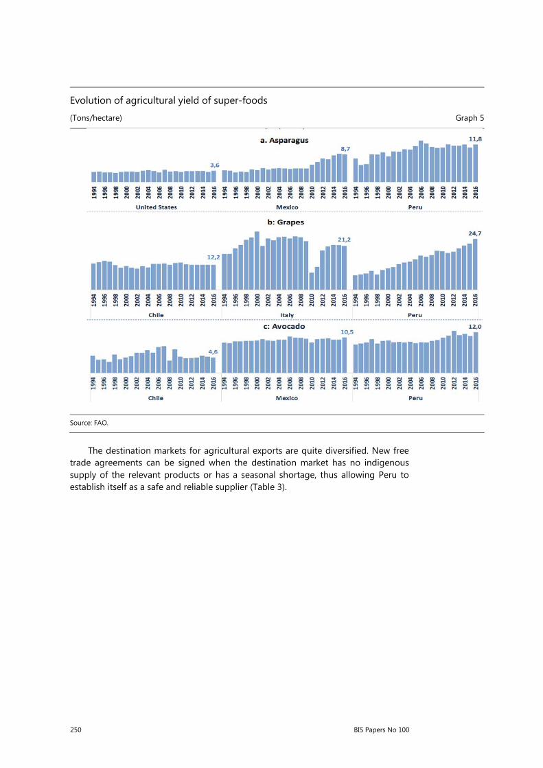
250 BIS Papers No 100
Evolution of agricultural yield of super-foods
(Tons/hectare) Graph 5
Source: FAO.
The destination markets for agricultural exports are quite diversified. New free
trade agreements can be signed when the destination market has no indigenous supply of the relevant products or has a seasonal shortage, thus allowing Peru to establish itself as a safe and reliable supplier (Table 3).

BIS Papers No 100 251
Agricultural exports by product and destination as of 2016 Table 3
Sources: Sunat.
Peruvian food exporters match their supply to the harvesting calendar of their competitors according to the harvesting schedule “window” as determined by weather conditions, seasonality and global demand. Figure a of Graph 6 and Table 4 show that Peruvian avocado exporters use a different “window” than Chileans, so that their exporting schedules are complementary. In the case of grapes (figure b) and blueberries (figure c) Peru has an earlier exporting season than Chile, which opens up market opportunities.10
Agricultural exports window, Peru-Chile (2011–17)
(Percentages of total world exports) Graph 6
Source: Sunat.
Peru is a significant secondary supplier of avocados to the US market. According
to Table 5, between 2011 and 2016 the US Haas avocado market increased from 516,000 tons to 1 million tons with an annual average growth of 15%. During the same period, California, the main US producer of avocadoes, increased its delivery
10 Vasquez et al (2017).
0
50
100
150
Jan.
11Ap
r.11
Jul.1
1O
ct.1
1Ja
n.12
Apr.1
2Ju
l.12
Oct
.12
Jan.
13Ap
r.13
Jul.1
3O
ct.1
3Ja
n.14
Apr.1
4Ju
l.14
Oct
.14
Jan.
15Ap
r.15
Jul.1
5O
ct.1
5Ja
n.16
Apr.1
6Ju
l.16
Oct
.16
Jan.
17
a: Fresh avocados
Chile Peru
0
100
200
300
Jan.
13M
ar.1
3M
ay.1
3Ju
l.13
Sep.
13N
ov.1
3Ja
n.14
Mar
.14
May
.14
Jul.1
4Se
p.14
Nov
.14
Jan.
15M
ar.1
5M
ay.1
5Ju
l.15
Sep.
15N
ov.1
5Ja
n.16
Mar
.16
May
.16
Jul.1
6Se
p.16
Nov
.16
Jan.
17M
ar.1
7
c: Blueberries
Chile Peru
0
200
400
600
Jan.
11Ap
r.11
Jul.1
1O
ct.1
1Ja
n.12
Apr.1
2Ju
l.12
Oct
.12
Jan.
13Ap
r.13
Jul.1
3O
ct.1
3Ja
n.14
Apr.1
4Ju
l.14
Oct
.14
Jan.
15Ap
r.15
Jul.1
5O
ct.1
5Ja
n.16
Apr.1
6Ju
l.16
Oct
.16
Jan.
17
b: Fresh grapes
Chile Peru

252 BIS Papers No 100
from 120,000 tons to 166,000 tons, with an annual average growth of 7%; Mexico, the main external supplier, increased its delivery from 318,000 tons to 780,000 tons, with an annual average growth of 20%; and Peru, the second most important external supplier of avocados to the United States, increased its delivery from 8,000 tons to 33,000 tons with an annual average growth of 34%.
Main agricultural export windows
(Millions of US dollars) Table 4
Source: Sunat.
Total Haas avocado deliveries to the US market
(In thousands of tons) Table 5
Source: Haas Avocado Board, under the supervision of the US Department of Agriculture.
The markets for avocados, asparagus and blueberries have experienced
important shifts during the last decade. Peru increased its share of US demand for avocados between 2000 and 2016, taking market share from other participants (Table 6). Also, the share of Peruvian blueberries in total US imports of blueberries has expanded by more than 10 percentage points, thanks to an increase in cultivated area and productivity improvements.

BIS Papers No 100 253
Shares of suppliers to the US market Table 6
Sources: USDA, USITC, Sunat.
Mining
The nationalisation of mining companies in the 1970s undercut the exploration, production and exports of all Peru’s main mineral products.11 Between 1970 and 1990, export volumes per inhabitant (kilograms/population) fell in the case of silver from 40 to 23, copper from 16 to 13 and zinc from 25 to 24. The following decade brought a price recovery that encouraged the start-up of new projects. This recovery was driven by the enactment of the General Mining Law in 1992, which encouraged private sector investment in the mining sector and established tax-stability contracts.12 The volume of mining exports has since grown steadily, except during the Great Financial Crisis (Graph 7). Based on the indicator of mining exports volumes per inhabitant, the improvement between 1990 and 2017 shows impressive results for gold (from 0.04 to 6), copper (from 13 to 83) and zinc (from 24 to 38). Peru also ranks highly in the world league tables of mineral producers (Table 7).
11 Glave and Kanamoto (2002).
12 By constitutional reform, two important elements were introduced to promote investment. On the one hand, foreign investment is eligible for the same treatment as local investment and a legally secure contractual framework was given to private contracts, including contracts for the development of mining projects.
2000 2016 2000 2016 2000 2016Mexico 16.7 91.3 Mexico 52.8 59.4 Chile 63.7 52.2Peru 0 3.7 Peru 41.3 39.7 Canada 22.4 16.1Chile 65.1 3.1 Canada 0 0.7 Peru 0 11.4Others 18.2 1.9 Others 0.1 0.1 Others 13.9 20.3
Avocados Asparagus Blueberries

254 BIS Papers No 100
Volume of mining exports in Peru
(Index 2007=100) Graph 7
Source: Central Reserve Bank of Peru.
Mineral prices rose almost continuously between 2002 and 2011, interrupted
only by the Great Financial Crisis. This price rise is linked to demand from China. Higher international prices promoted mining investment in Peru, supporting output. Graph 10 relates the changes in copper prices to China’s annual GDP growth rate since 2002.
Mining products Table 7
Sources: Comtrade, ITC.
2017
Zinc 2,022 1Silver 637 1Copper 11,998 2Lead 1,069 2Molybdenum 367 4Tin 370 5Gold 7,096 6
(Millions of US$)
World ranking

BIS Papers No 100 255
The risks to exports of commodities are associated more with the state of the Chinese economy than any trend towards greater protectionism (Graph 8). Additionally, mining projects demand significant imports of machinery and equipment from developed economies. Table 8 shows the main imports of Peru from the United States and exports from Peru: risk levels are low due to the low percentage of manufactured exports from Peru.
China’s GDP vs copper export prices
(Annual growth rates) Graph 8
Sources: WEO and Sunat.
Other exports
As strong momentum of mining exports may obscure trends in other exports, it is worth noting that from 2000 to 2017 the number of export products rose from 3,454 to 4,227 and that the number of destination countries increased from 156 to 174. This trend can be explained by the consolidation of macroeconomic stability, structural reforms to boost efficiency and productivity and the free trade agreements.
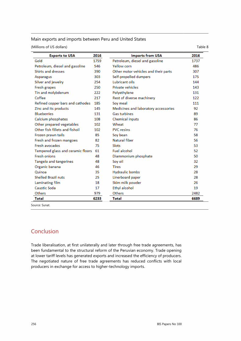
256 BIS Papers No 100
Main exports and imports between Peru and United States
(Millions of US dollars) Table 8
Source: Sunat.
Conclusion
Trade liberalisation, at first unilaterally and later through free trade agreements, has been fundamental to the structural reform of the Peruvian economy. Trade opening at lower tariff levels has generated exports and increased the efficiency of producers. The negotiated nature of free trade agreements has reduced conflicts with local producers in exchange for access to higher-technology imports.

BIS Papers No 100 257
References
Abusada, R, J Illescas and S Taboada (2001): Integrando el Perú al Mundo, Universidad del Pacífico, Instituto Peruano de Economía.
Baier, S and J Bergstrand (2007): “Do free trade agreements actually increase members’ international trade?”, Journal of International Economics, vol 71, pp 72–95.
Cespedes, N, M Aquije, A Sanchez and R Vera-Tudela (2014): “Productividad y tratados de libre comercio a nivel empresas en Perú”, DT No 2014-014, Central Reserve Bank of Peru.
Glave, M and J Kanamoto (2002): “La minería peruana: lo que sabemos y lo que aún nos falta saber”, Lima: GRADE, pp 135–81.
Ross, K and J Peschiera (2015): “Explaining the Peruvian growth miracle, IMF”, in A Santos and A Werner (eds), Peru, Staying the Course of Economic Success, pp 37–50.
Vasquez, C, R Morales and M Puch (2017): “Exportaciones no tradicionales en los últimos 5 años: el boom agroexportador”, Moneda, no 172, Central Reserve Bank of Peru.

258 BIS Papers No 100

BIS Papers No 100 259
The globalisation experience and its challenges for the Philippine economy1
Diwa C Guinigundo2
Abstract
This paper analyses the extent and impact of globalisation in the Philippines in terms of trade, finance and migration. In the Philippines, trade globalisation and migration have been more prominent than financial globalisation. While empirical estimates show that globalisation has positively affected the country’s economic growth and employment, substantial evidence for its impact on inequality and poverty has yet to be found, as preliminary estimates show mixed results. There are both winners and losers among industries and in the labour market. Thus, more inclusive policies could potentially help cushion the negative consequences of globalisation and facilitate adjustments to narrow the gap between winners and losers. Towards this end, the Bangko Sentral ng Pilipinas has made contributions primarily through its focus on low and stable inflation; the facilitation of greater financial inclusion; and greater involvement in global cooperation efforts to further strengthen rule-based international transactions.
Keywords: impact of globalisation, challenges of globalisation, policy response to globalisation, migration, remittances, financial inclusion, Philippines.
JEL classification: F6, F62, F63, F66, F68, F22, F24.
1 A paper prepared for the Bank for International Settlements (BIS) Emerging Markets Deputy
Governors Meeting, 8–9 February 2018, Basel, Switzerland. The usual institutional disclaimer applies.
2 Deputy Governor, Monetary Stability Sector, Bangko Sentral ng Pilipinas
260 BIS Papers No 100
1. Introduction
Globalisation is defined as the mobility across borders of goods and services, people, capital and knowledge (BIS (2017a)). In the past half century, the world economy has become much more integrated, interdependent and intertwined as globalisation and liberalisation appear to have become an inevitable and irreversible trend. Regional trading arrangements, the removal of restrictions on the flow of trade and investment, and rapid technological changes have led to the deepening of economic integration and the heightening of globalisation (Aldaba (2011)). Emerging market economies (EMEs) have also become much more tightly integrated in terms of trade, finance, global value chains (GVCs) and migration (BIS (2017b)).
Some have attributed an unprecedented period of peace and prosperity to globalisation as it has spurred growth and productivity as well as expanding opportunities for businesses, investors and workers (Ibrahim (2017)). This is true particularly for EMEs, where many observers consider globalisation as a major cause of strong growth and significant poverty reduction in recent decades (BIS (2017b)). However, due to the adverse and lingering impact of the Great Financial Crisis (GFC), there has been a growing backlash against globalisation, not only in EMEs but also in advanced economies, particularly in the United Kingdom and the United States. A pattern of resurgent protectionism is observed to be emerging across the globe and inward-looking policies are getting more support.
This paper analyses how globalisation has affected the Philippines, starting with globalisation trends in the country (Section 2), and followed by macroeconomic and distributional consequences of globalisation (Section 3). The paper continues with a discussion on challenges that the country faces with greater world integration (Section 4), and finally with a discussion of policies in the last section (Section 5).
2. Globalisation trends in the Philippines
The Philippine economy, like that of most other EMEs, has become increasingly integrated with the global economy. This is evident in the general increase in trade in goods and labour migration. There is also greater integration in finance, albeit at a relatively moderate pace.
Trade openness
From the 1990s to the 2000s, trade openness in the Philippines improved from 88.1% to 101.0% of the country’s gross domestic product (GDP) (Graph 1). Contributing to this increase were the country’s efforts towards a more open trade policy starting in the 1980s. This trade openness also reflected declining transport costs and improved information and communications technology that supported the development of complex GVCs, particularly in electronics and electrical components, allowing companies to manage their production more efficiently (Dudley (2017)).

BIS Papers No 100 261
Economic globalisation indicators (% of GDP), 1990s, 2000s, 2010s Graph 1
Note: Trade openness = [(Exports of goods and services + Imports of goods and services)/Real GDP] x 100; Financial Openness = [(Inflows of direct investment, portfolio investment, financial derivatives and other investment + Outflows of direct investment, portfolio investment, financial derivatives and other investment)/Nominal GDP] x 100. Figures from 1990 to 1999 were based on BOP Old Concept. Figures from 2000 to 2004 were based on BPM5. Figures from 2005 to 2017 were based on BPM6. 2010s include January to September 2017 data for financial openness and January to December 2017 data for trade openness. Estimates exclude valuation changes. The analysis, however, should be taken with caution considering the break in the data series used (old, BPM5 and BPM6 concepts).
Sources: National Accounts, Philippines Statistics Authority; BOP Statistics and International Investment Position, Bangko Sentral ng Pilipinas.
Another factor is rapid growth in the information and communications technology-business process outsourcing (ICT-BPO) services in the country. Based on data on earnings from IT-BPO, the industry recorded above 50% annual growth from 2006 to 2008, this growth remaining in double digits until 2016. The Philippines has also established itself as one of the two major BPO industry centres in Asia, along with India. With the country’s continued openness to globalisation, the total trade of the Philippines increased further, to 101.4% of GDP in the 2010s (Graph 1). The pickup in global trade starting in 2017 has, in fact, helped in offsetting the weak global demand that lingered after the GFC.
Financial openness
In terms of financial openness, globalisation came in at a more moderate pace. The country’s total capital flows increased from 3.1% of GDP in the 1990s to 3.4% of GDP in the 2000s (Figure 1). While the Philippines started to liberalise the foreign exchange (FX) regulatory system in the 1990s, capital inflows were dampened by the Tequila (Mexican peso) financial crisis in 1995 and the Asian financial crisis in 1997–98 (Tetangco (2005)).
In the 2010s, however, total capital flows rose to 4.6% of GDP. This could be attributed in part to the nine waves of FX liberalisation reforms undertaken by the BSP starting in 2007. Another important reform undertaken to promote financial openness was the further liberalisation of foreign bank entry in 2014. Notwithstanding this, the 4.6% average ratio of capital flows to GDP from 2010 to the

262 BIS Papers No 100
first three quarters of 2017 indicates that there is still scope for the country to liberalise further.3
The composition of the economy’s external liabilities has shown its increasing exposure to both portfolio and direct investments, signifying not merely foreign investors’ search for yield but growing confidence in the country’s macroeconomic fundamentals (Graph 2). From end-December 1999 to end-September 2017, the stock of foreign direct investments (FDI) increased by 816.9%.4 As a share of GDP, FDI has increased from 9.6% at end-1999 to 23.5% at end-September 2017. Relative to GDP, FPI has increased from 18.7% at end-December 1999 to 25.8% at end-September 2017.
Moreover, external assets show a sustained increase in foreign exchange reserves from 18.2% of GDP at end-December 1999 to 26.2% of GDP at end-September 2017 (Graph 3), reflecting large and stable structural flows coming from overseas Filipino remittances and IT-BPO receipts. Notable also is the substantial increase in residents’ direct investments abroad, from only 0.8% of GDP at end-December 1999 to 14.9% of GDP at end-September 2017. Residents’ portfolio investments in other countries likewise increased from 1.5% of GDP in end-December 1999 to 5.2% at end-September 2017, signifying the rising internationalisation of domestic corporates and investors.
3 Based on IMF (2017), while the Philippines made a significant progress in liberalising capital flows in the past 10 years, foreign exchange market development and interbank market in the country are still below potential.
4 The cited figure is the computed growth rate of the stock of FDI in end-September 2017 from end-December 1999. The data are based on International Investment Position, a stock statistic.
External liabilities, 1999–Q3 2017 Graph 2 External assets, 1999–Q3 2017 Graph 3
(% of GDP, end-period) (% of GDP, end-period)
Note: External assets and liabilities data are based on International Investment Position (stock data). For end-1999 and end-2000, the data were estimated using Balance of Payments (BOP) statistics figures for 2000 and 2001, respectively. Figures from end-2001 to end-2005 were based on BPM5. Figures from end-2006 to end-September 2017 were based on BPM6. Estimates exclude valuation changes. The analysis, however, should be taken with caution considering the break in the data series used (relating to the BPM5 and BPM6 concepts).
Sources: National Accounts, Philippines Statistics Authority; BOP Statistics and International Investment Position, Bangko Sentral ng Pilipinas.

BIS Papers No 100 263
Migration
International migration from the Philippines increased further as data from the United Nations indicate that the ratio of Filipino migrants to the country’s total population went up from 3.5% in 1995 to 5.4% in 2017,5 and the ratio of the stock of overseas Filipinos to the country’s total population increased from 9.4% in 1997 to 10.4% in 2013.6
The Philippines has been open to labour mobility since the 1970s, and this has provided the country with decades of experience as a source of international migrants. The primary reason for Filipinos’ continued emigration has been to seek employment overseas. While the Philippine economy has been steadily improving in recent years, with unemployment rate declining from 7.5% in 2009 to 5.0% in 2017, the country’s unemployment situation7 is still commonly cited as one of the main reasons why Filipinos continue to search for work abroad.8 Employment opportunities in other countries, regardless of the type of job, are perceived to offer higher salaries/compensation, and better income and lifestyle packages (eg health benefits, insurance).
Another set of factors that promoted greater labour mobility pertains to global events that enhanced the international migration opportunities of Filipinos, particularly in extending their workplace to a global scale. For instance, the adoption of more liberal immigration policies in the 1970s; the oil crisis of 1973 that facilitated the emergence of the Gulf region as a destination for temporary migrant workers; the rise of the new industrialised countries in East and Southeast Asia that spurred additional demand for migrant labour in the 1980s; and globalisation have all led to global demand for skilled and professional workers.
Lastly, labour migration has been explained by so-called contagious migration. This refers to the widespread interest in migration that has resulted from the influence of the growing number of migrants. This seems to have become a social construct that is now ingrained in Philippine culture. For instance, migration seems to be transmitted within families from one generation to the next.9
5 Figures were estimated using United Nations (UN) data on the stock of migrants from the Philippines and estimates of the Philippine Statistics Authority on latest population of the Philippines. The UN defines the stock of migrants as the number of people born in a country other than that in which they live (Source: United Nations, Department of Economic and Social Affairs, Population Division (2017)).
6 Figures were estimated using data from the Commission on Filipinos Overseas on stock of overseas Filipinos (latest data are 2013) and the estimates of the Philippine Statistics Authority on the current population of the Philippines.
7 According to the Department of Labor and Employment (DOLE), the unemployment problem in the country is not just about the lack of jobs, but also includes the mismatch between the human capital portfolio of job applicants and the requirements of the labour market. The business process outsourcing (BPO) sector, for instance, is having difficulties in finding qualified workers.
8 Pinoy OFW Portal, “Eight Reasons why many Filipinos want to work abroad”, www.pinoy-ofw.com/news/355-reasons-why-many-filipinos-like-to-work-abroad.html.
9 The motivation to improve the family’s welfare and status led either parents or their children to migrate abroad – for parents, it is to provide a better future for their children, whereas for the children, migration is seen as a means of providing a comfortable life for their parents. There is a dissemination and sharing of information that encourages migration. The tendency for migration to spread from
264 BIS Papers No 100
Based on the latest estimate from the Commission on Filipinos Overseas, overseas Filipinos (OFs) are now scattered more geographically, from the traditional destinations, comprising mostly the advanced economies, to EMEs, which have been increasingly tapping OF services and skills.10 The profile of Filipino migrants has also changed from mostly middle and lower skilled workers (1970s) to professional workers (1990s) as well as services (2000s and 2010s) and production workers (2010s) (Ang et al (2009)).
As a result, the remittances sent by OFs have substantially increased, from 2.5% of GDP in 1990 to 9.2% of GDP in the first three quarters of 2017. The Philippines was the third highest recipient country for remittances in 2017 and has been in the top 10 since 1994 (World Bank (2017a)). In recent years, the BSP and the banks themselves have adopted various measures to encourage OFs to channel remittances through the financial system, following improvements in international money transfer technology (Bayangos (2012)).
3. Macroeconomic and distributional impacts of globalisation in the Philippines
While the foregoing trends show continuing trade, migration, and financial integration of the Philippines, an unintended consequence is the greater exposure of the country’s domestic economy to migrant returns and volatility spillovers from other countries’ equity markets. However, the country’s participation in the globalised world of trade, finance and migration has resulted in tangible benefits, including low and stable inflation, a low unemployment rate, more than adequate gross international reserves, and a sound and fundamentally strong banking system.
3.1 Economic growth and employment
Evidence suggests that globalisation has a positive effect on the country’s economic growth and employment. In particular, trade openness and foreign portfolio flows have contributed to higher per capita GDP growth in the Philippines, following the implementation of FX liberalisation reforms. A significant increase in OF remittances has raised consumption, investment, labour productivity and economic growth. These OF remittances have also supported the Philippine economy during normal times and crisis situations in the past, and this is expected to continue in the future (Ang et al (2009)).
Moreover, FDI increases employment growth and gross value added, not just in the manufacturing sector itself but in other sectors as well, including construction,
one municipality to a neighbouring one exhibits the spillover effects of information. The aspirations of youngsters are moulded by the examples of migrants, especially in areas where poverty and conflict are present (Abrigo and Desierto (2011)).
10 While the United States still holds the largest share of total resident OFs, its share of the total has declined from 37.2% in 2005 to 34.5% in 2013. The OF population in the Middle East grew from a share of total stock of 23.5% in 2005 to 24.3% in 2013.
BIS Papers No 100 265
financial intermediation, and transport, storage, and communication.11, 12 Also, the sustained growth in employment and salaries obtained from the global offshore IT-enabled services industry over the years has greatly increased household spending and investments (Del Prado (2015)).
3.2 Inflation
In addition to the country’s credible and efficient implementation of inflation targeting (Guinigundo (2017)), globalisation is also considered as one of the factors for the observed decline in the sensitivity of inflation in the Philippines to changes in real economic activity or the flattening of the Phillips curve. On the one hand, a flatter Phillips curve implies that demand shocks and policy errors will not translate into large inflation movements. On the other hand, this means that, if inflation is above target, bringing it down to the target level would entail a greater sacrifice of output, giving greater weight to the central bank’s commitment to its primary responsibility for price stability (Guinigundo (2017)).
This attribution is based on three observations of Iakova (2007). First, strong international competition constrains businesses from increasing prices when demand rises. Second, increased trade and investment flows have made prices less responsive to domestic demand pressures. Third, global migration, which has intensified in recent years, has caused wages and prices to become less sensitive to domestic demand shifts. These apply to the Philippines’ exports or imports, which have become less concentrated (concentration index declined from 0.36 in 1995 to 0.29 in 2016, with 1 as highly concentrated) and the country has also reduced its divergence from world trade patterns (diversification index dropped from 0.62 in 1995 to 0.56 in 2016, with 1 as greatly divergent).13 The former indicates the presence of more diversified products, and more competition in the domestic market, while the latter implies that the export/import structure of the Philippines is becoming less different from that of world trade.14
3.3 Poverty alleviation and income inequality
A recurring concern related to increasing globalisation is its impact on poverty alleviation and income inequality. Preliminary estimates show that an increase in trade openness contributes to reduction in income inequality in the Philippines, such that a 1 unit increase in the trade-to-GDP ratio can reduce the Gini coefficient by 0.04 unit.15 By contrast, OF remittances contribute to higher income inequality as for every
11 Based on Granger causality test between manufacturing FDI growth and sectoral employment growth
for the period Q1 2006–Q4 2016 (Santos and Oliva (2018)).
12 FDI likewise has a long-run relationship with employment growth and gross value added growth in almost all sectors.
13 Based on the United Nations Conference on Trade and Development (UNCTAD) data from 1995 to 2015.
14 With the country’s increasing import volumes, this also means global developments exert a greater influence on the domestic market. As in Cacnio (2013), in fact, trade openness has contributed considerably to the flattening of the Phillip’s curve (ie more than migration has).
15 Bayangos (2015).

266 BIS Papers No 100
1 unit increase in the ratio OF remittances to GDP, the Gini coefficient increases by 3.3 units. Estimates also show that trade openness has no significant impact on poverty, although OF remittances can help reduce poverty.16
It is worth noting that, while there is evidence that higher rates of growth can reduce poverty (Dollar et al (2013)), if GDP growth is accompanied by an increase in inequality, this could still worsen poverty. According to Bourguignon (2004), both growth and inequality changes play a major role in generating changes in poverty. He explains that, over the medium run, distributional changes may be responsible for sizeable changes in poverty and in some instances, these changes may even offset the favourable effects of growth. This was supported by a study conducted in the Philippines by Reyes and Tabuga (2011), in which they found that, while the rate of growth matters a lot in poverty reduction, the redistribution of income also matters.17 This implies that the nature of economic growth matters. While globalisation has no direct impact on poverty, globalisation can affect poverty indirectly through its impact on economic growth and income inequality.
4. Challenges of increasing globalisation
While globalisation has reportedly strengthened the global economy and improved welfare in general, the literature indicates that the distribution of its benefits in many countries has been uneven18 and some acknowledge its potential role in fuelling the rising trend towards income inequality.19 In the case of the Philippines, no substantial evidence for the impact of globalisation on inequality and poverty has so far been found. Nevertheless, there are winners and losers in globalisation, which could affect the country’s economic and social development. Moreover, the country faces challenges from uncertain global factors exacerbated by the possible revival of protectionism. These events could lead to greater volatility and risk-averse attitudes among the country’s trade and investment partners.
4.1 Firms, labour market and distribution of gains for growth
In particular, industries that are less able to compete and workers whose skills have become less relevant may be adversely affected and will have difficulty in adjusting due to globalisation. According to Sibal (2005), firms that were among the losers in the globalisation process in the Philippines were mostly in the small and medium categories in agriculture (eg producers of vegetables, palay, corn and poultry), sunset industries and labour-intensive firms (eg garments and apparel). The share of agriculture to GDP declined from 16.4% in 1980 to 8.5% in 2017 while that of industry fell from 41.6% in 1980 to 34.1% in 2017. In the industrial sector, the shares to GDP
16 As in the poverty regression model in Bayangos (2015).
17 Bourguignon (2004).
18 Dudley (2017).
19 BIS (2017b). Other central banks, however, conclude that trade liberalisation reduced earnings discrepancies, while others stress that skill-biased technological change, and not trade globalisation per se, is responsible for divergence.

BIS Papers No 100 267
of textile manufactures and wearing apparel declined from 1.3% and 1.4%, respectively, in 1998 to 0.3% and 0.4%, respectively, in 2017. These firms need to upgrade their technologies and improve production efficiency and productivity to be able to compete.
On the other hand, emigration can be a catalyst for improvement in the quality of the labour force in the short term as it can push individuals to improve their skills so that they can eventually emigrate.20 This could also lead eventually to “brain gain,” where OF workers bring the knowledge they learned abroad back to their home country.
4.2 Greater exposure to external shocks and policies
Another challenge posed by globalisation is greater economic exposure to destabilising external forces due to greater financial openness. Unless sufficient safeguards are in place, financial openness accompanied by poor regulation can threaten financial stability (BIS (2017c)).
Based on a 2015 IMF report, an abrupt shift in market expectations could expose the Philippines to a spike in interest rates, with negative feedback effects on the real economy. Moreover, the IMF observes that the country’s local currency government bond yields are strongly influenced by global factors. Since these serve as benchmarks for pricing corporate bonds, they could have a wide-ranging impact on the country’s real economy.
Meanwhile, due to the Philippines’ high degree of trade integration and significant role in international migration, the country is likely to be affected by external noise mainly through OF remittances, offshoring/outsourcing, and trade channels. For instance, if we are to consider the current concerns about US policies regarding globalisation, and if the United States pursues deglobalisation policies that could result in a lower US GDP growth rate by 1 percentage point, this is expected to reduce the Philippine real GDP growth rate by 0.06 percentage points in the first year and by 0.07 percentage points in the second year. The country’s inflation rate would decline by an estimated 0.01 percentage points in the first year and by 0.03 percentage points in the second year. Meanwhile, if deglobalisation policies were to require the United States to increase its Federal Funds rate, a 1 percentage point hike would have no estimated effect on the Philippine’s economic growth in the first year but it would lead to a 0.02 percentage point reduction in the second year. But it would result in an estimated 0.02 percentage point increase in the Philippine inflation rate in the first year and a 0.11 percentage point increase in the following year.21
The Philippines has also been affected by other countries’ policies through the remittance channel. OF remittances have recently been affected by de-risking activities or stricter regulatory measures enforced by various countries in compliance with the Financial Action Task Force – Guidance on the Risk-Based Approach for Money Services Businesses (FATF-RBA). These de-risking activities of international banks, particularly in reference to the Anti-Money Laundering and Countering the Financing of Terrorism Act, have led to the closure of bank accounts maintained with
20 OECD/Scalabrini Migration Center (2017).
21 Based on estimates of the Department of Economic Research of the Bangko Sentral ng Pilipinas.
268 BIS Papers No 100
international banks by both bank-owned and stand-alone remittance companies/money transfer operators (MTOs) in the Philippines in the past two years.
It may be noted that five of the 14 countries22 affected by de-risking in 2015 showed declines in remittances in US dollars. The decline, however, may not be attributed solely to the effect of de-risking, but also to other factors such as currency depreciation. In the case of the Philippines, the decline in remittances in the original currency of the host countries may be an indication of the impact of de-risking in these countries.
5. Policy responses to the challenges
The solution to the challenges brought by globalisation is not a rollback of globalisation arising from protectionism since this could lead only to greater challenges resulting from other costs and distortions, such as lower economic growth, a higher inflation rate, and disruption in GVCs and job losses.23 Instead, more inclusive policies will help cushion the negative consequences of globalisation and facilitate the adjustment in narrowing the gap between the winners and losers. Workers need some retooling to help them find new well-paying jobs and for producers to be more productive and internationally competitive.24 For the Philippines, the National Government could work with the private sector and civil society groups on local initiatives that provide technology and skills to disadvantaged groups such as in barangays within and outside the cities (Roldan (2010)). In the case of Filipino migrants, there is a need to protect their rights and well-being as well as to facilitate their participation in the country’s development, particularly during reintegration. Like other central banks, the BSP needs to better understand the implications of globalisation on the performance of the economy, inflation and financial stability.25
5.1 The BSP’s contribution
5.1.1 Promote low and stable inflation
For its part, the BSP has helped to maintain stable and low inflation, which supports domestic economic stability, encouraging investments and business expansion, which, in turn, fuels employment growth. From August 2015 to October 2017, inflation for the bottom 30% of households by income was lower, in general, than inflation for all income households or headline inflation. The BSP has likewise ensured that the country’s domestic liquidity conditions, external position, and financial system and creditworthiness remain healthy with the aim of further raising investor confidence.
22 Austria, France, New Zealand, the United Kingdom and the United States. This is based on the analysis
of the Department of Economic Statistics of the Bangko Sentral ng Pilipinas. The 14 countries that are being monitored by the Anti-Money Laundering Steering Group include the United States, Singapore, the United Kingdom, Canada, Hong Kong SAR, Australia, New Zealand, Italy, Papua New Guinea, Brunei, Austria, Cyprus, Saipan and France.
23 BIS (2017b).
24 Dudley (2017).
25 BIS (2017b).

BIS Papers No 100 269
However, in the Philippines, the majority of the population do not have access to formal finance. Thus, a large segment of the population has no access to credit. The key challenge, therefore, is to develop mechanisms that would allow the poor access to formal finance and credit, enabling them to finance productive activities and investments, and thus participate in and contribute to economic growth.
5.1.2 Promote financial inclusion
The BSP has been deeply involved in initiatives that promote financial inclusion to ensure that appropriate financial products and services are accessible to a great majority of the population.
For instance, in 2008, the BSP developed the Credit Surety Fund Program (CSF), which has helped micro, small and medium-sized enterprises (MSMEs) grow their business. As of end-December 2017, there were 51 operating CSFs in the country with loans approved amounting to about PHP 4.6 billion. The BSP likewise allowed the establishment of micro banking offices (MBOs) in 2010, which have increased outreach in areas that are unbanked from 251 MBOs in 2011 to 839 in the third quarter of 2017.
The BSP has also promoted the offering of microfinance loans, micro agricultural loans, microfinance housing loans, micro-deposits and micro-insurance. As of the third quarter of 2017, there were 164 banks with microfinance operations serving more than 1.8 million clients with a loan portfolio amounting to PHP 14.8 billion. In 2013, the BSP allowed non-bank agents (such as pawn shops, grocery stores, and drug stores) to perform electronic money (e-money) transactions, such as remittances and payments.
The National Financial Inclusion Strategy was launched in July 2015, which highlights the importance of technology in facilitating fund transfers and expanding the reach of financial institutions to unserved and underserved areas. Also in 2015, the BSP launched the National Retail Payment System (NRPS) with the goal of developing a seamless payments and settlements highway. As of end-September 2017, there were 26,028 e-money agents in the country, or a 195% growth from 8,819 e-money agents in end-December 2010.
A nationwide Economic and Financial Learning Program aims to educate OFs and their families about the importance of using remittances to build up savings and directing these into investments in financial products and/or business ventures.
The BSP continues to create a supportive policy environment for financial inclusion by harnessing technology towards digital financial inclusion. While significant gains in the area of financial inclusion have been achieved over the years, the challenge is to further scale up the reach of financial services to cover an even greater number of people, with the expectation that this will help reduce poverty and income inequality, and further promote economic growth.
5.1.3 Cooperation in global efforts to further strengthen rules-based international transactions
Meanwhile, countries should also work together to further strengthen the global rules-based system (eg trade facilitation agreements, level playing field in trade and tax), the joint regulatory approach to properly manage global financial risks, and international cooperation and regional integration, particularly for issues like climate

270 BIS Papers No 100
change and cyber-security. There is also a need for international cooperation in helping migrants become socially integrated in host countries and to help reduce remittance costs.26 International policy coordination is needed on the implementation of AML/CFT rules consistent with global standards to facilitate the development of collective regulatory expectations or possible arrangements for cross-border recognition of AML/CFT compliance. For this case, the BSP has raised the issue with the Alliance for Financial Inclusion, the Global Partnership for Financial Inclusion (GPFI) of the G20, the Financial Stability Board, the World Bank and the United States Treasury.
26 National Economic and Development Authority, “Philippine Development Plan, 2017-2022,” NEDA,
Pasig City, 2017.

BIS Papers No 100 271
References
Abrigo, M and D Desierto (2011): “Contagious migration: evidence from the Philippines”, Philippine Institute for Development Studies, Discussion Paper Series, no 2011-18.
Aldaba, R (2011): “Globalization, competition, and international production networks: policy directions for the Philippine automotive industry”, Philippine Institute for Development Studies, Policy Notes, no 2011-13, June.
Ang, A, G Sugiyarto and S Jha (2009): “Remittances and household behavior in the Philippines”, ADB Economics Working Paper Series, no 188, December.
Bank for International Settlements (2017a): “Globalisation and de-globalisation”, Outline of issues for the meeting of Deputy Governors on 8–9 February 2018, 19 September.
——— (2017b): “Globalisation: an emerging market perspective”, Note for the meeting of Governors from major emerging market economies, 10 September.
——— (2017c): 87th Annual Report, June.
Bayangos, V (2012): “Going with remittances: the case of the Philippines”, BSP Working Paper Series, no 2012-01, July.
——— (2015): “Monetary policy and income inequality”, Hitotsubashi University and the IMF Joint Seminar on Inequality: What has been happening, why does it matter, and what needs to be done?, 12–13 March, Tokyo, Japan.
Bourguignon, F (2004): “The poverty-growth-inequality triangle”, The World Bank.
Cacnio, F (2013): “Analysing inflation dynamics in the Philippines using the new Keynesian Phillips curve”, Philippine Review of Economics, vol 50, no 2, December, pp 55–83.
Commission on Filipinos Overseas (2013).
Del Prado, F (2015): “The BPO challenge: leveraging capabilities, creating opportunities”, Philippine Institute for Development Studies, Discussion Paper Series, no 2015-36, July.
Dollar, D, T Kleineberg and A Kraay (2013): “Growth is still good for the poor”, World Bank Policy Research Working Paper, no 6568, August.
Dudley, W (2017): “Benefits and challenges for globalization”, remarks for the Bombay Stock Exchange, 11 May.
Guinigundo, D (2017): “Implementing flexible inflation targeting in the Philippines”, Philippine Central Banking: A Strategic Journey to Stability, BSP.
Hasan, R and K Jandoc (2010): “Trade liberalization and wage inequality in the Philippines”, ADB Economics Working Paper Series, no 195, March.
Iakova, D (2007): “Flattening of the Phillips curve: implications for monetary policy”, IMF Working Paper Series, no 07/76, April.
Ibrahim, M (2017): “Some perspectives on globalisation and its aftermath”, International Monetary Fund-Bank Negara Malaysia Summer Conference, Kuala Lumpur, July.
272 BIS Papers No 100
International Monetary Fund (2015): “Philippines: Selected Issues”, IMF Country Report, no 15/247, September.
——— (2017): “Aide memoire on capital account liberalization and foreign exchange market development”, October.
International Organization for Migration (2013): Country migration report: the Philippines.
Medalla, E and M Mantaring (2009): “On free trade agreements (FTAs): The Philippine perspective”, Philippine Institute for Development Studies, Discussion Paper Series, no 2009-35, December.
OECD/Scalabrini Migration Center (2017): “Interrelations between public policies, migration and development in the Philippines”, OECD Development Pathways, OECD Publishing, Paris.
Philippine Statistics Authority, National Accounts of the Philippines (2017).
Reside, R (2009): “Determinants of overseas Filipino worker remittances”, UP School of Economics Discussion Papers, University of the Philippines.
Roldan, M (2010): “Globalization and glocalization: experiences in the local Philippine context”, Philippine Institute for Development Studies, Discussion Paper Series, no 2010-21, October.
Sander, C (2003): “Migrant remittances to developing countries”, paper prepared for the UK Department of International Development (DFID), June, pp 1–41.
Santos, H and M Oliva (2018): “An analysis of foreign direct investments in the Philippines and ASEAN”, BSP Working Paper Series, forthcoming.
Sibal, J (2005): “The effects of globalization and economic restructuring on Philippine labor policies and the responses of the actors of the Philippine industrial relations system”, Paper presented at International Society of Labour and Social Security Law (ISLSSL), Eighth Asian Regional Congress, Taiwan.
Tetangco, A (2005): “The composition and management of capital flows in the Philippines”, BIS Papers, no 23.
United Nations, Department of Economic and Social Affairs, Population Division (2017): “Trends in international migrant stock: The 2017 revision documentation”, December.
World Bank (2017a): “Annual remittances data”, October.
——— (2017b): “Remittance prices worldwide”, issue 24, December.
BIS Papers No 100 273
Globalisation and the Polish economy: macro and micro growth effects
Piotr Szpunar and Jan Hagemejer1
Abstract
We analyse the macro and micro effects of globalisation in Poland. We show that exports were a major contributor to economic growth in the transition period and after the 2004 EU enlargement. While exporting and foreign capital are associated with faster productivity growth at the sector level, we show that internationalised firms, both through exporting and foreign direct investment, perform better than non-internationalised firms. While this difference in performance between firms as well as a sizeable premium in capital/labour ratio manifest themselves in a large difference in average wages, we show that labour productivity-adjusted wages are in fact lower in exporters than in non-exporters, which can be associated with downward competitive pressure on wages.
Keywords: internationalisation, productivity, growth, wages.
JEL classification: L25, F23, F15, O12.
1 Piotr Szpunar, Director, Department of Economic Analysis, Narodowy Bank Polski.
Jan Hagemejer, Head of Structural Analysis Unit, Narodowy Bank Polski, corresponding author, [email protected]. The views presented here are those of the authors and do not necessarily reflect the official position of the NBP.

274 BIS Papers No 100
Introduction
Globalisation is associated with increased trade flows and foreign direct investment. From the 1990s, in addition, production processes have been fragmented through outsourcing and offshoring. The pattern of trade has gradually changed from 19th century inter-industry trade, where the advanced economies produced manufactured goods and the emerging market economies (EMEs) produced basic goods to a pattern where manufacturing is located in both advanced economies and EMEs and, instead of specialisation in products, countries specialise in different production tasks and processes. Specialisation is designed to improve production efficiency and hence can lead to productivity growth and improvements in factor allocation (see eg Baldwin (2014)).
In Poland and other central and eastern European countries, the process of integration with the global economy overlapped with the transition process and later with the EU accession. Opening up involved not only access to foreign markets but also the inflow of foreign direct investment. FDI provided capital that was scarce in the transforming economies and it helped build their export potential. At the same time, access to modern technologies and improved organisational structures, know-how, labour discipline and corporate culture have helped to expand exports and contribute to overall economic growth.
The emergence of trading firms within EMEs may potentially polarise a country’s economy. The modern globalised sector flourishes due to technological advancements and productivity growth while traditional sectors (or non-tradable sectors) lag behind (McMillan and Rodrik (2011)). The trade literature finds grounds also for within-sector variation in productivity. Melitz (2011)-type models postulate self-selection mechanisms that allow only the most productive firms to enter export markets (due to the fixed costs of exporting) while less productive firms either sell to the domestic market only or exit. Alternatively, firms may learn from participation in export markets (learning-by-exporting) and gradually increase productivity after entering foreign markets (see for example Bernard and Jensen (1999), De Loecker (2013) and Hagemejer (2017) for early evidence for Poland).
Foreign direct investment can have direct productivity effects through access to modern technology and managerial procedures. As documented by many authors those direct effects can be exaggerated due to selection issues (foreign investors invest in better firms, see for example Greenaway and Kneller (2007), and Hagemejer and Tyrowicz, (2012)). Apart from these direct effects, there is a broad empirical evidence that suggests indirect productivity benefits. As shown in a meta-analysis by Havranek and Irsova (2011), they mostly take a form of backward spillovers, ie domestic firms supplying intermediate goods and services to foreign and multinational firms benefit from productivity improvements. In this vein, the related literature provides systematic empirical evidence in favour of the importance of spillovers for CEE countries. Finally, in the context of the Polish economy, Hagemejer and Kolasa (2011) document that there are significant productivity spillovers from firm internationalisation and more importantly, that this empirical regularity is robust to a choice of measure of international activity (hosting FDI, exporting and importing of investment goods).
In this paper, we show, using the results from two recent papers by Hagemejer (2017) and Hagemejer and Mućk (2017) that between 1995 and 2014 exports were responsible for more than half of overall economic growth. Then we turn to sector-

BIS Papers No 100 275
and firm-level analysis to show that exporting and foreign direct investment are indeed associated with higher productivity, faster productivity growth and better factor allocation. Within sectors, firm internationalisation is additionally associated with higher average wages, thus contributing to the dispersion of income in the economy. We also show that foreign and exporting firms have systematically lower productivity-adjusted average wages, which may stem from the necessity of sustaining cost-competitiveness.
Export led-growth in central and eastern Europe and Poland
Fragmentation of production processes may lead to a misinterpretation of gross trade statistics. In order to produce a final good, intermediate goods may cross borders several times. At each stage, exports require significant amount of imports and hence only a small fraction of gross exports contributes to the GDP of the exporting country by creating domestic value added. The net exports contribution to GDP growth is misleading, since both imports and exports contain intermediate and final goods and at the same time the final demand aggregates in GDP have a varying import intensity. In particular, in EMEs, investment demand is import-intensive and hence raw net exports contributed negatively to the GDP growth of CEE countries throughout much of the transition period.
Decomposition of value added growth Graph 1
Sources: Hagemejer, (2017), Hagemejer and Mućk, (2017). The “domestically absorbed” bar corresponds to the growth in value added that is generated in production of goods and services and finally absorbed by domestic final demand. The “absorbed abroad” bar corresponds to the growth in value added that is consumed as part as foreign domestic demand. The two bars sum up to overall domestic real value added growth.
In order to overcome this measurement problem, Kranderdonk and Verbruggen (2005) correct for the varying import intensity of final demand components based on input-output tables. Given the availability of yearly World Input Output Tables, Hagemejer (2017) proposes instead to use the Johnson and Noguera (2012)

276 BIS Papers No 100
decomposition of overall GDP to value added that is absorbed domestically and the one that is exported – hence providing a direct accounting of the GDP contribution from exports.
As Graph 1 shows, in Poland and in other CEE countries, exports have been the predominant driver of economic growth for most of the period analysed, from 1995 to 2014. This reflects an increasing export specialisation in the CEE countries, ie that an increasing share of output was directed towards exports. At the same time final demand has become increasingly dependent on imports. In Poland, the contribution of exports to overall value added output is, in relative terms, lower than elsewhere due to a larger domestic market than in other CEE countries. However, the greater diversification of Polish exports has helped Poland to maintain higher export growth following the Great Financial Crisis (GFC) than other economies in the region.
As shown by Hagemejer (2017), on average around 60% of CEE exports are intermediate goods. Trade in intermediate goods is associated with the activity of global value chains, ie these intermediate goods are further processed elsewhere along the GVC. One can decompose the changes in the share of world exports to parts attributable (i) to the growth of domestic value added (contribution of exports to domestic GDP) and (ii) to foreign value added, indicating the changes in the trade value that are driven by the process of production relocation and offshoring. Such a decomposition is shown in Graph 2 for 2000–14. While the gain in German market share was due solely to offshoring to other countries (including the CEE), in Poland and other CEE countries it was also driven by the contribution of domestic value added.
Decomposition of changes in market share 2000–14, manufacturing Graph 2
Source: Hagemejer and Mućk (2017. The figure shows the decomposition of a change in the world’s exports to parts that are attributable to domestic value added growth and foreign value added growth (import intensity of exports).
-2
-1.5
-1
-0.5
0
0.5
1
FR DE CZ HU PL SKDomestic value added Foreign value added Change in export market share

BIS Papers No 100 277
Exports, foreign ownership and productivity at the sector level
In order to look more closely at the role of exports and FDI in shaping economic activity in Poland, we explore a rich firm-level data set from the Polish Central Statistical Office that covers all firms with 10 or more employees. It includes data from the profit and loss statements as well as the balance sheet, which is complemented by information on the form of ownership of every firm. Due to important changes in the structure of the data set, we are able to look at aggregate measures starting from 2002 but the consistent sectoral breakdown of the data is available starting from 2005, the year of Poland’s EU accession.
As shown in Graph 3, foreign firms were responsible for a large share of the value added generated in the economy as well for a large share of employment. In 2015 these shares amounted to more than 32% and 38%, respectively. Since 2002, these numbers have been growing fast. The corresponding share of exporters in the overall sample are more volatile due to firms exiting and entering the exporter category (we take a threshold of 10% of revenues to classify firms as exporters to exclude firms that export sporadically and in very small amounts). However, in 2015 the shares of exporters in employment and value added were of about the same magnitude as the ones for foreign enterprises. FDI is also closely related to exporting, in particular in the tradable sector – manufacturing – where highly export-oriented sectors are also dominated by firms with foreign capital. Notable exceptions include beverage production (sector 112), where foreign capital is predominant but the industry is geared towards the domestic market, as well as apparel (14) and furniture (31), which are export-oriented but comprise mostly domestic firms.
Share of foreign firms in overall economy (left), export shares of revenues and foreign firm shares in value added in manufacturing (right) Graph 3
Source: Authors’ calculations using firm-level data. Numbers in the scatter plot in right panel refer to NACE rev. 2 sectors (listed in Appendix B.
In line with the literature, the internationalisation of firms and sectors of production is associated with higher labour productivity. This regularity is more pronounced in the case of foreign ownership (Graph 3, right-hand panel) rather than
2 NACE rev. 2 sector codes are listed in Appendix B.

278 BIS Papers No 100
exporting. Outliers include such sectors as chemicals (20) as well as pharmaceuticals (21) that are capital-intensive and also involve non-tangible assets in production, as well as beverage production (11), which, as noted above, is domestic-market oriented but has a large share of foreign firms.
The 10-year real growth rates of labour productivity (Graph 11 in the Appendix) reveals a similar pattern and shows a robust association between sector internationalisation and labour productivity growth. There are, however, two outstanding sectors where the scale of labour productivity growth was the highest in the period analysed: the food sector and beverage production. In both of these sectors labour productivity increased threefold. While both of these sectors are geared mainly towards the domestic market, the food sector is the largest manufacturing sector in Poland and, given its size, is among the top exporting sectors.
Labour productivity levels and sector internationalisation, 2015 Graph 4
Source: Authors’ calculations using firm-level data. Numbers in scatter plots refer to NACE rev. 2 sectors (listed in Appendix B.
Allocative efficiency (OP-gaps) and sector internationalisation Graph 5
Source: Authors’ calculations using firm-level data.

BIS Papers No 100 279
According to Olley and Pakes (1996), sector-level (employment-weighted) labour productivity can be decomposed to firm-level (unweighted) labour productivity and the covariance component between firm size and productivity (the so-called OP-gap). The covariance component can be understood as the measure of allocation of resources, ie the larger the (positive) covariance, the more efficient is the allocation of resources (more productive firms grow larger). A negative covariance term is associated with resource misallocation. Graph 5 shows the OP-gap measure for the manufacturing sectors, which turns out to be positive for all sectors and shows a positive relationship between sectoral internationalisation and allocative efficiency.
Internationalisation, firm-level productivity and wages
In order to inquire into the intra-sectoral effects of globalisation, we follow Bernard and Jensen (1996) and estimate simple regressions of the form:
ln(𝑋𝑋𝑖𝑖) = 𝛼𝛼 + 𝛽𝛽𝛽𝛽𝛽𝛽𝑡𝑡𝑖𝑖 + 𝛾𝛾𝛽𝛽𝛽𝛽𝛾𝛾𝛾𝛾𝛾𝛾𝑡𝑡𝛾𝛾𝑦𝑦𝑖𝑖 + 𝜀𝜀𝑖𝑖 , where the 𝑋𝑋𝑖𝑖 variable is a performance indicator (labour productivity, TFP3,
average wage, capital-labour ratio), 𝛽𝛽𝛽𝛽𝑡𝑡𝑖𝑖 is a firm-level internationalisation dummy (exporting or foreign ownership) and 𝛽𝛽𝛽𝛽𝛾𝛾𝛾𝛾𝛾𝛾𝑡𝑡𝛾𝛾𝑦𝑦𝑖𝑖 are the industry fixed effects. We estimate such cross-sectional regressions for every year between 2005 and 2015 for the overall sample of firms and for manufacturing, with and without the industry fixed effects (for manufacturing only with fixed effects). We concentrate on the estimates of 𝛽𝛽 showing the approximate percentage differences in the 𝑋𝑋𝑖𝑖 between internationalised and non-internationalised firms. Graphs 6–9 and 11 (in the Appendix) are all constructed in the same manner. The “Overall economy” line corresponds to the level of the 𝛽𝛽 estimates without any sectoral controls, the “Controlling for sector differences” line shows the 𝛽𝛽 estimated for all firms in a regression including two-digit sector fixed-effects and “Manufacturing” shows the estimates of 𝛽𝛽 in that sector controlling for two-digit sectors in manufacturing.
Labour productivity differences (in percent): exporter vs non-exporters (left), foreign vs domestic firms (right) Graph 6
Source: Authors’ calculations using firm-level data
3 We estimate firm-level total factor productivity with the Levinsohn-Petrin (2003) method, using
materials to control for unobservables. In order to produce TFP estimates comparable across sectors, we restrict the capital and labor parameters to be the same across all sectors.

280 BIS Papers No 100
Graph 6 shows the comparison of labour productivity levels between exporters and non-exporters (left-hand panel) and foreign and domestic firms (right-hand panel). One can see that these differences are sizeable and they greatly differ depending on the sample analysed and the method of comparison. The exporter productivity premium turns out to be almost 35% in manufacturing and in the overall sample by the end of the period analysed after controlling for sector specificity. When these controls are not included, differences stemming from the intersectoral variation of productivity are not only greater but also increase over time. The productivity premia of foreign firms over domestic enterprises are more stable over time and they range from about 40% in manufacturing to considerably more for the overall sample. Similar patterns can be observed for TFP differences (Graph 12 in the Appendix). Appendix Table 1 and 2 show the exporter and foreign productivity premia for exporters and foreign firms estimated on a sample pooled for 2005–15 and show that, while the foreign firm productivity advantage is higher than that of exporters, these premia are not additive, ie some of the advantage foreign firms have over domestic firms comes from the fact that they tend to be exporters at the same time.
The exporter and foreign firm labour productivity advantage comes from the facts that internationalised firms have higher total factor productivity and that they also tend to have more capital per worker. These differences are shown in Graph 7. While in the productivity comparison a large part of the productivity difference was due to inter-sectoral differences, the differences between internationalised and non-internationalised firms tend to be larger within sectors than across sectors and they are considerably higher in manufacturing than elsewhere, ie export participation in manufacturing involves a capital-labour ratio that is higher by almost 70% in manufacturing and by 40–50% overall. Foreign firms are also likely to have more capital than domestic firms but, unlike in the case of exporters, this advantage seems to be fading out over time.
Capital/labour ratio differences (in percent): exporter vs non-exporters (left), foreign vs domestic firms (right) Graph 7
Source: Authors’ calculations using firm-level data.
Large differences in productivity and K/L ratios between internationalised and non-internationalised firms lead to large wage differences. While we do not control specifically for the skill premium of labour, the sector-level fixed effects should take care of the inter-sectoral differences in skill requirements. Wage differences between exporters and non-exporters exhibit a different pattern than do those of foreign and

BIS Papers No 100 281
domestic firms. In the case of the former comparison, differences between sectors are less important than differences in wages within sectors, which amount to roughly 25% of the wage premium of exporters vs non-exporters and seem to have gone up after the GFC. While for the overall economy the foreign firm wage premium is large and amounts to a stable 50% even after controlling for sector specificity, it is considerably lower in manufacturing (35%). Overall, both the increasing exporter wage premium and the increasing importance of foreign firms affect overall wage growth in Poland as well as aggravating income inequality.
In order to inquire further into the wage premia from internationalisation, we normalise the wage level by labour productivity and regress the log of this ratio on the internationalisation dummy variables to understand to what extent labour is remunerated in line with its productivity. The coefficient of the internationalisation dummies for all years under consideration is presented in Graph 9. It shows that productivity-adjusted wages are significantly lower for exporters than for non-exporters after the GFC by 5–10%. This result stems from two possible sources: (i) the cost-price competitiveness of exporters that keeps wage growth below the growth rate of productivity and (ii) persistently higher capital share of value added by exporters than by non-exporters. While this phenomenon is present in exporters both in manufacturing and in the overall sample, in the case of foreign-domestic firms comparison the pattern is similar only in manufacturing, ie the tradable sector. In the overall sample, the wage/productivity ratio is higher for foreign firms than for domestic firms suggesting that in non-tradable sectors the downward competitive pressure on wages is lower than in manufacturing (see also Table 5 for estimates for the pooled sample and standard errors).
Average wage differences (in percent): exporter vs non-exporters (left), foreign vs domestic firms (right) Graph 8
Source: Authors’ calculationss using firm-level data.

282 BIS Papers No 100
Wage/productivity ratio differences (in percent): exporter vs non-exporters (left), foreign vs domestic firms (right) Graph 9
Source: Authors’ calculations using firm-level data.

BIS Papers No 100 283
Conclusions
We provide empirical evidence on the contribution to economic growth of participation in export markets and foreign direct investment. We show that, throughout much of the transition period, the post-accession period and after the GFC, exports have been a major growth driver for direct value added. This finding applies to Poland and to some extent to other CEE countries. The post-crisis differences in growth performance stem from a different pattern of specialisation in exports, ie Poland’s exports focus to a larger extent on consumption goods and intermediates used in the production of such goods.
We show, using Polish firm-level data, that firms’ participation in export markets and in hosting foreign direct investments is also related to productivity growth and productivity level differences. Productivity growth is due to the processes taking place in firms: ie productivity gains of firms with foreign capital through adoption of modern technology and managerial improvements, as well as the learning-by-exporting of domestic exporters. Additionally, FDI inflows and exporting are associated with a higher degree of allocative efficiency, ie resources are re-allocated to more productive firms.
However, participation in global markets has its distributional consequences. Sectors that engage in trade are more productive than others and firms that export have a productivity premium over firms focused on the domestic market. However, productivity differences translate to wage differences only to some extent. While exporters and foreign firms pay higher wages than non-exporters and domestic firms do, the productivity-adjusted wage premium of exporters has been negative, in particular after the GFC. One possible reason for this persistent difference is the necessity for exporters to maintain their price-cost competitiveness.
A question for future research is how far export-driven growth is sustainable in the longer run. Poland and other CEECs have enjoyed sizeable productivity improvements thanks mainly to FDI substituting for domestic innovation and capital As such, the export growth model has been based on price-cost competitiveness and proximity to markets. Future wage growth in the export-oriented segment will depend on how far the the country can shift towards higher value added goods and services, creating its own global value added chains and outward FDI, thus gaining additional shares in global markets. Those improvements can be facilitated by a predictable institutional environment as well as appropriate innovation-oriented incentives to enterprises.

284 BIS Papers No 100
References
Baldwin, R (2014): “Trade and industrialization after globalization’s second unbundling: how building and joining a supply chain are different and why it matters”, in R Feenstra and A Taylor (eds), Globalization in an age of crisis: multilateral economic cooperation in the twenty-first century, University of Chicago Press, pp 165–212.
Bernard, A and J Jensen (1999): “Exceptional exporter performance: cause, effect, or both?”, Journal of International Economics, vol 47, no 1, pp 1–25.
De Loecker, J (2013): “Detecting learning by exporting”, American Economic Journal: Microeconomics, vol 5, no 3, pp 1–21.
Greenaway, D and R Kneller (2007): ”Firm heterogeneity, exporting and foreign direct investment”, Economic Journal, vol 117, no 517, pp F134–F161.
Hagemejer, J (2017): “Trade and growth in the new member states. The role of global value chains”, Emerging Markets Finance and Trade, (forthcoming).
Hagemejer, J and J Mućk (2017): “Unravelling the economic performance of the CEE countries: the role of exports and GVC”, mimeo, Narodowy Bank Polski.
Hagemejer, J and J Tyrowicz (2012): “Is the effect really so large? Firm-level evidence on the role of FDI in a transition economy”, The Economics of Transition, vol 20, no 2, pp 195–233.
Hagemejer, J and M Kolasa (2011): “Internationalisation and economic performance of enterprises: evidence from Polish firm-level data”, The World Economy, vol 34, no 1, pp 74–100.
Havranek, T. and Irsova, Z. (2011), “Estimating vertical spillovers from FDI: Why results vary and what the true effect is”, Journal of International Economics, vol. 85, no 2, pp. 234-244
Johnson, R and G Noguera (2012): “Accounting for intermediates: Production sharing and trade in value added”, Journal of International Economics, vol 86, no 2, pp 224–36.
Kranendonk, H. and Verbruggen, J. (2008): “Decomposition of GDP Growth in Some European Countries and the United States”, De Economist, vol. 156, no 3, pp. 295-306.
Olley, G and A Pakes (1996): “The dynamics of productivity in the telecommunications equipment industry”, Econometrica, vol 64, no 6, pp 1263–97.
Levinsohn, J and A Petrin (2003): “Estimating production functions using inputs to control for unobservables”, Review of Economic Studies, vol 70, no 2, pp 317–41
McMillan, M and D Rodrik (2011): “Globalization, structural change and productivity growth”, NBER Working Papers, no 17143, National Bureau of Economic Research.

BIS Papers No 100 285
Appendix A – additional figures and tables
Total factor productivity levels, 2015 Graph 10
Source: Authors’ calculations using firm-level data. Numbers in scatter plots refer to NACE rev. 2 sectors (listed in Appendix B.
Labour productivity growth Graph 11
Source: Authors’ calculations using firm-level data. Numbers in scatter plots refer to NACE rev. 2 sectors (listed in Appendix B.

286 BIS Papers No 100
Total factor productivity differences (in percent): exporter vs non-exporters (left), foreign vs domestic firms (right) Graph 12
Source: Authors’ calculationss using firm-level data.
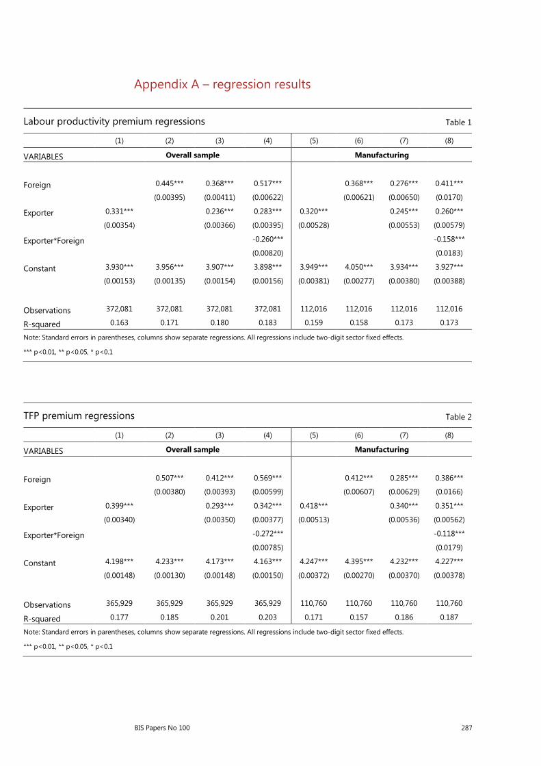
BIS Papers No 100 287
Appendix A – regression results
Labour productivity premium regressions Table 1
(1) (2) (3) (4) (5) (6) (7) (8)
VARIABLES Overall sample Manufacturing
Foreign 0.445*** 0.368*** 0.517*** 0.368*** 0.276*** 0.411***
(0.00395) (0.00411) (0.00622) (0.00621) (0.00650) (0.0170)
Exporter 0.331*** 0.236*** 0.283*** 0.320*** 0.245*** 0.260***
(0.00354) (0.00366) (0.00395) (0.00528) (0.00553) (0.00579)
Exporter*Foreign -0.260*** -0.158***
(0.00820) (0.0183)
Constant 3.930*** 3.956*** 3.907*** 3.898*** 3.949*** 4.050*** 3.934*** 3.927***
(0.00153) (0.00135) (0.00154) (0.00156) (0.00381) (0.00277) (0.00380) (0.00388)
Observations 372,081 372,081 372,081 372,081 112,016 112,016 112,016 112,016
R-squared 0.163 0.171 0.180 0.183 0.159 0.158 0.173 0.173
Note: Standard errors in parentheses, columns show separate regressions. All regressions include two-digit sector fixed effects.
*** p<0.01, ** p<0.05, * p<0.1
TFP premium regressions Table 2
(1) (2) (3) (4) (5) (6) (7) (8)
VARIABLES Overall sample Manufacturing
Foreign 0.507*** 0.412*** 0.569*** 0.412*** 0.285*** 0.386***
(0.00380) (0.00393) (0.00599) (0.00607) (0.00629) (0.0166)
Exporter 0.399*** 0.293*** 0.342*** 0.418*** 0.340*** 0.351***
(0.00340) (0.00350) (0.00377) (0.00513) (0.00536) (0.00562)
Exporter*Foreign -0.272*** -0.118***
(0.00785) (0.0179)
Constant 4.198*** 4.233*** 4.173*** 4.163*** 4.247*** 4.395*** 4.232*** 4.227***
(0.00148) (0.00130) (0.00148) (0.00150) (0.00372) (0.00270) (0.00370) (0.00378)
Observations 365,929 365,929 365,929 365,929 110,760 110,760 110,760 110,760
R-squared 0.177 0.185 0.201 0.203 0.171 0.157 0.186 0.187
Note: Standard errors in parentheses, columns show separate regressions. All regressions include two-digit sector fixed effects.
*** p<0.01, ** p<0.05, * p<0.1

288 BIS Papers No 100
K/L premium regressions Table 3
(1) (2) (3) (4) (5) (6) (7) (8)
VARIABLES Overall sample Manufacturing
Foreign 0.365*** 0.240*** 0.330*** 0.619*** 0.410*** 0.583***
(0.00826) (0.00860) (0.0130) (0.0108) (0.0113) (0.0297)
Exporter 0.450*** 0.389*** 0.417*** 0.669*** 0.558*** 0.577***
(0.00736) (0.00768) (0.00828) (0.00917) (0.00962) (0.0101)
Exporter*Foreign -0.158*** -0.202***
(0.0172) (0.0321)
Constant 3.506*** 3.570*** 3.491*** 3.485*** 3.286*** 3.531*** 3.264*** 3.255***
(0.00316) (0.00280) (0.00320) (0.00325) (0.00664) (0.00484) (0.00663) (0.00678)
Observations 374,452 374,452 374,452 374,452 110,763 110,763 110,763 110,763
R-squared 0.226 0.223 0.228 0.228 0.160 0.145 0.170 0.171
Note: Standard errors in parentheses, columns show separate regressions. All regressions include two-digit sector fixed effects.
*** p<0.01, ** p<0.05, * p<0.1
Average wage premium regressions Table 4
(1) (2) (3) (4) (5) (6) (7) (8)
VARIABLES Overall sample Manufacturing
Foreign 0.486*** 0.441*** 0.566*** 0.338*** 0.277*** 0.393***
(0.00272) (0.00283) (0.00423) (0.00373) (0.00390) (0.0102)
Exporter 0.254*** 0.140*** 0.181*** 0.236*** 0.160*** 0.173***
(0.00251) (0.00254) (0.00274) (0.00321) (0.00331) (0.00347)
Exporter*Foreign -0.223*** -0.135***
(0.00563) (0.0110)
Constant 3.552*** 3.552*** 3.525*** 3.518*** 3.421*** 3.482*** 3.406*** 3.400***
(0.00105) (0.000911) (0.00103) (0.00105) (0.00232) (0.00166) (0.00228) (0.00233)
Observations 397,696 397,696 397,696 397,696 112,012 112,012 112,012 112,012
R-squared 0.184 0.225 0.231 0.234 0.189 0.208 0.224 0.225
Note: Standard errors in parentheses, columns show separate regressions. All regressions include two-digit sector fixed effects.
*** p<0.01, ** p<0.05, * p<0.1

BIS Papers No 100 289
Wage/productivity premium regressions Table 5
(1) (2) (3) (4) (5) (6) (7) (8)
VARIABLES Overall sample Manufacturing
Foreign 0.0416*** 0.0710*** 0.0542*** -0.0268*** 0.00282 -0.0131
(0.00283) (0.00295) (0.00440) (0.00403) (0.00425) (0.0111)
Exporter -0.0741*** -0.0923*** -0.0979*** -0.0779*** -0.0787*** -0.0804***
(0.00254) (0.00265) (0.00286) (0.00342) (0.00361) (0.00378)
Exporter*Foreign 0.0301*** 0.0186
(0.00587) (0.0120)
Constant -0.464*** -0.486*** -0.469*** -0.468*** -0.414*** -0.451*** -0.414*** -0.413***
(0.00106) (0.000946) (0.00107) (0.00109) (0.00247) (0.00179) (0.00248) (0.00254)
Observations 397,677 397,677 397,677 397,677 112,008 112,008 112,008 112,008
R-squared 0.082 0.081 0.084 0.084 0.055 0.051 0.055 0.055
Note: Standard errors in parentheses, columns show separate regressions. All regressions include two-digit sector fixed effects.
*** p<0.01, ** p<0.05, * p<0.1
Appendix B – NACE rev. 2 sector codes, manufacturing
Code Description 10 Manufacture of food products 11 Manufacture of beverages 12 Manufacture of tobacco products 13 Manufacture of textiles 14 Manufacture of wearing apparel 15 Manufacture of leather and related products 16 Manufacture of wood and of products of wood and cork, except furniture; manufacture of articles
of straw and plaiting materials 17 Manufacture of paper and paper products 18 Printing and reproduction of recorded media 19 Manufacture of coke and refined petroleum products 20 Manufacture of chemicals and chemical products 21 Manufacture of basic pharmaceutical products and pharmaceutical preparations 22 Manufacture of rubber and plastic products 23 Manufacture of other non-metallic mineral products 24 Manufacture of basic metals 25 Manufacture of fabricated metal products, except machinery and equipment 26 Manufacture of computer, electronic and optical products 27 Manufacture of electrical equipment 28 Manufacture of machinery and equipment n.e.c. 29 Manufacture of motor vehicles, trailers and semi-trailers 30 Manufacture of other transport equipment 31 Manufacture of furniture 32 Other manufacturing 33 Repair and installation of machinery and equipment

290 BIS Papers No 100

BIS Papers No 100 291
Globalisation and deglobalisation
Bank of Russia
Abstract
We argue that, as emerging market economies (EMEs) gradually converge with advanced economies, the advantages they gain from participating in trade and global value chains (GVCs) have lessened, resulting in lower growth in world trade post-crisis. But EMEs can sustain their long-term growth by participating in the higher value-added and more complex parts of GVCs.
Protectionism is an increasing threat to future global economic growth. The solution lies largely in addressing inequality and fostering structural transformation. Based on Russia’s experience, we conclude that an optimal policy mix for a commodity-exporting EME consists of a floating exchange rate, inflation targeting, a fiscal rule, and macroprudential policy.
Keywords: global value chains, globalisation, international trade, Russia.
JEL classification: D63, E58, F02, F41, F60.
A. Determinants of international trade and population flows
What explains the growth of international trade in EMEs in recent years? Is weak trade growth in the aftermath of the Great Financial Crisis a temporary phenomenon or does it mark a new trend?
The main contributing factors to the rapid growth of trade in the current century have been:
A large demographic dividend in the major EMEs. This served as the impetus for the inclusion of these countries into global value chains (GVCs) as assemblers of labour-intensive products.
The reduction of transport costs through containerisation and the automation of port and production logistics. Cost reduction exercised a non-linear (increasing) effect on trade at the start of globalisation.1
The development of regional and global integration (via WTO accession), which, by reducing import tariffs, has had a profound effect on the growth of world trade.
Industrialisation has supported EMEs’ income growth and their participation in GVCs not only as suppliers of production factors (labour, cheap natural resources), but as buyers of final and intermediate products, including those of other EMEs.
1 See, P Krugman, “A finger exercise on hyperglobalisation”, blog post, New York Times, June 2017, https://krugman.blogs.nytimes.com/2017/06/14/a-finger-exercise-on-hyperglobalization/.

292 BIS Papers No 100
Importantly, EMEs have strongly contributed to global economic growth, expanding south-south trade (ie trade among EMEs) faster than north-south trade (ie trade between EMEs and advanced economies). This was also the case for Russia. The share of Russian exports to China, Korea and India saw a significant increase between 2003 and 2016, reflecting the declining share of trade with advanced economies, the EU in particular. See Graph 1 in the Appendix.
Research has shown2 that the slowdown of world trade since 2011 has been most pronounced for trade in goods. The slowdown was accompanied by a reduction in GVC participation by both EMEs and advanced economies. This was seen most markedly in the reduced share of complex value chains in GVCs.
The global trade slowdown since 2011 has been caused primarily by:
- The upsurge in protectionism to support the recovery of national economies after the Great Financial Crisis (GFC) in both EMEs and advanced economies, including through changes in the real currency exchange rates of advanced relative to emerging market economies.
- The replacement of imported intermediate goods (processing trade) with domestic goods in the largest EMEs. Industrialisation enabled developing countries to replace external with internal supply chains. This was the case with Chinese metal production, which has emerged as a competitor to Russian suppliers.
- Technical progress also allowed participation in GVCs to be replaced with domestic alternatives. Robotisation in advanced economies has reduced the cost not only of low-skilled labour, but medium-skilled labour as well, redirecting some production back to the United States, for example. The US shale revolution, meanwhile, is reshaping the global oil market.
- Changes in EME growth models. EMEs are seeing their economies increasingly rebalanced towards services in the context of rising incomes and a reduced demographic dividend. The younger generation is characterised by higher levels of education, which has helped certain EMEs to compete with developed countries in innovation.
On the whole, the gradual convergence of EMEs with advanced economies (in income levels, productivity, capital-to-labour ratio and innovation) indicates that the advantages that these countries reap from trade and participation in GVCs are irreversibly and permanently on the decline. This has reduced world trade growth below its pre-crisis levels. Reduced protectionism could exert a temporary but significant stimulating effect on world trade due to non-linearity (high marginal return).
For a better understanding of the outlook for world trade, it is necessary to examine the trends and prospects of GVC formation.
2 See the survey in World Bank (2017) and Figure 2.7 in the report.

BIS Papers No 100 293
Will global value chains (GVCs) continue to lengthen or has this process reached a natural limit? Which factors determine the degree of integration into GVCs and how does this affect trade?
The integration of countries in GVCs is based on several factors:
− Logistical advantages. The WTO identifies a direct link between a country’s logistical advantages and its involvement in GVCs.3 In order to participate in a GVC, it is better to be a coastal country than one in the heart of a continent (for example, Korea vs Mongolia). In this respect, Russia, despite possessing the largest territory, is in a disadvantageous position as it has access to predominantly northern seas, remote from the main trade routes. This partly explains Russia’s low Logistic Performance Indicator.4
− Location near the largest trade hubs: China, Europe and the United States. Thus, the presence of large neighbours strongly increases a country’s chances of active participation in GVCs. For example, the United States fulfils that function for Mexico, as does China for New Zealand or Russia. Russia’s advantage lies in its proximity to two large trade hubs: Europe and China.5 This determines the main orientation of the country’s trade flows.
− A surplus of certain resources. With respect to labour, for instance, a key role is played not by low wages in themselves, but unit labour costs (ULC), that is, wages with productivity taken into account. Low labour productivity in the majority of African countries together with relatively high wages (large African countries suffer from “Dutch disease”) is a major barrier to their inclusion into GVCs. For Russia, a similar abundant factor is natural resources, particularly gas and oil. This determines the nature of the country’s participation in GVCs.
− The institutional environment (the openness of the economy, standards of business protection) and the accessibility of trade finance. These factors are especially important for the formation of complex chains, in which component goods cross borders many times. The relevant figures for most EMEs have room for improvement.
Thus, the growth of world trade is primarily contingent upon increased country participation in long (complex) value chains. The factors indicated above have negatively affected the length of value chains (see Graph 2), and thus, world trade.
The prospects of GVC development will determine world trade performance. There are extensive and intensive GVC growth factors. Extensive factors include the expansion of geographic coverage, the involvement of small and medium-sized enterprises (SMEs) in GVCs, and the development of GVCs in services.
First, geographically, African and South Asian countries could play an important role in GVC growth. Their inclusion in GVCs is constrained by low labour productivity and lack of capital even for labour-intensive sectors. Automation and robotisation in advanced economies and EMEs reduce the likelihood that these countries will be
3 World Bank (2017).
4 According to the World Bank index, in 2016 Russia occupied 99th place out of 160 countries. Germany, Sweden, the Netherlands, Singapore, Austria, the United Kingdom and the United States occupied the top places.
5 Sanghi et al (2017).

294 BIS Papers No 100
included in GVCs, as compared with the inclusion of East Asian countries in GVCs 20 years ago.
Second, for SMEs, the impetus for GVC development has increased, thanks to reduced transaction costs in gaining access to external markets due to the partial elimination of information asymmetry (thanks to IT counterparty search platforms) and of liquidity constraints (via trade finance instruments and risk insurance). The advance of IT in logistics lowers the risks of production delays for these businesses.
Third, GVC development in service production has vast growth potential. Besides, GVC development in services has positive externalities for GVC growth in the production of goods. Yet, GVC development in services faces high protectionist barriers in financial, medical, industrial and educational services. With respect to the role of GVC in services, the question is how one should evaluate the participation of foreign banks, insurance companies and other financial intermediaries in generating a country’s GDP: can potential risks outweigh potential benefits? Or is there no such trade-off?
Thus, the prospects of extensive GVC development are not straightforward. Special economic zones within EMEs, such as the one in the Russian Far East, are one way of embedding EMEs in GVCs.
As for intensive factors of GVC development, EMEs that are integrated into existing GVCs have already received most of the resultant benefits. Indeed, several EME countries face the challenge of the middle-income trap, and some attendant risks to financial stability.
Maintaining GDP growth in these EMEs requires a transition to a different growth model based on innovation and structural reforms in economies, so that they can participate in the higher value added parts of GVCs. But this is more difficult to achieve than their initial entry into GVCs. This task is also very relevant for Russia.
In addition, the diminishing marginal effect from late-20th century innovations such as containerisation and logistics automation does not enable further accelerated GVC creation. No profound new breakthroughs capable of lowering transport costs are foreseen.
Consequently, the slowdown in the growth of GVCs is likely to be a long-term phenomenon.
Unlike most EMEs, Russia entered the period of GVC development without a demographic dividend but it does have rich natural resources, which have supported Russia’s integration into the global economy.
Russia’s specialisation as a supplier of natural resources has grown in the past 20 years. See Graph 3 for an indication of its comparative advantage.
The growth of Russia’s specialisation was first and foremost attributable to rising demand from EMEs and advanced economies for raw commodities and their rising prices, and the effects of “Dutch disease” on Russia. Kilian (2009) shows that strong global demand was a dominant driver of crude oil price growth in 2000–07. “Dutch disease” (increasing wages in the tradable and non-tradable sectors) undermined the country’s competitiveness vis-à-vis central and eastern European countries. In addition, the development of Southeast Asian countries as centres of manufacturing reduced the role of light industry and other traditional labour-intensive sectors of the Russian economy. As a result, Russia was largely left on the sidelines of GVC

BIS Papers No 100 295
formation, specialising predominantly in forward participation (that is, exports of commodities used for further processing in importing countries) (Graph 4).
Russia’s competitive advantages include an abundance of natural resources, highly skilled labour, a vast territory, transport opportunities that must be further exploited (particularly considering the non-linear effect of transport costs), for example, development of the Northern Sea Route.
An insight into Russia’s changing role in GVCs may be found by looking at the experience of countries with similar demographics (Finland), and dependency on oil exports (Norway), which are both more firmly embedded in GVCs than Russia. This is particularly important in the light of technological innovations (such as shale oil and gas, alternative energy) that could weaken Russia’s position as a supplier of traditional raw materials in the long term. Changes in Russia’s role in GVCs will have important consequences for current trade partner countries as well. China’s rebalancing and the growth of the Indian economy are two additional factors that will affect the inclusion of Russia in GVCs.6
Why do some EMEs trade much more than others? To what extent have regional and global arrangements driven trade? How concerned are you about a return to protectionism and how would it affect EM trade integration?
The factors that drive trade between EMEs or regional trade are not altogether different from global trade factors. The only significant difference is the importance of protectionism, which is a more important factor on a regional than on the global level. On the global level, geographical factors, factors of proximity to large trade hubs, and the availability of cheap resources play a more important role for trade than on the regional level. In addition, studies show that reduced bilateral trade due to protectionism causes negative externalities for countries that are not directly affected by these reductions.
Russia is a big country with many neighbours. Regional free trade agreements are very important; agreements with growing, developing markets are valuable. A key question is whether countries aspiring to strengthen their positions in GVCs should develop internal production linkages between regions, and between neighbouring countries? Or can inclusion in GVCs develop without enhanced internal or regional integration? In this regard, Russia has benefited from the formation of the Eurasian Economic Union (EAEU), a regional production and trade association.
Russia’s role in the EAEU is not limited to trade in natural resources. The structure of Russian trade is visibly different from that of non-CIS economies (Table 1). Specifically, Russia has a higher share of processed goods in exports to the EAEU countries than in exports to the rest of the world.
The global rise of protectionism could have a damaging effect on world trade and Russia. The 2014 oil price shock prompted structural changes in the Russian economy that ran counter to those that occurred prior to the GFC. Specifically, both relative prices and the economic structure moved in favour of the tradable sector. Among other things, such structural changes opened up the non-commodity export
6 Sanghi et al (2017).

296 BIS Papers No 100
potential that had previously been blocked by the high real exchange rate. This makes Russia a natural proponent of globalisation.
In discussing the threats of protectionism, it is important to understand its nature. Advanced economies resent the transfer of manufacturing employment to EMEs. As a result, blue-collar workers either lose their jobs or are forced to tolerate lower wages. EMEs are concerned by their narrow specialisation in labour-intensive production. They are denied access to high value-added production (technological components, marketing, design). In this context, technological innovations lead to growing inequality in both advanced economies and EMEs. In such circumstances, protectionism and populism are the corresponding defensive reaction of the global economy to the absence of effective mechanisms for the structural reallocation of redundant production factors. Robotisation is set to further exacerbate these trends.
Therefore, the solution to the problem of protectionism lies largely in solving the problem of inequality and fostering structural transformation.
What are the drivers of migration flows into and out of EMEs? What has been the impact of migration on the size and composition of the workforce in EMEs? What drives remittances?
Adverse demographic trends require Russia to compete actively for global migration flows. Otherwise, even maintaining its existing production capacity will prove highly problematic.
Drivers of labour migration to Russia include:
− The higher level of dollar wages in Russia relative to other countries in Europe (Poland) and Asia (China) before the 2014 crisis.
− The inflow of migrants from culturally and historically close regions (eg the former Soviet republics).
There are sources of labour migration to Russia (Graph 5):
(i) Inflows of cheap, low-skilled labour from Central Asian countries increased greatly in the 2000s on the back of rising oil prices and the growth of dollar wages in Russia. They became outflows with the depreciation of the rouble at the end of 2014. Remittances from Russia also fell (Graph 6).
(ii) Inflows of medium-skilled labour from Ukraine and Moldova were stable in the 2000s, but reversed after the rouble depreciation in 2014 and amidst economic recession. Exacerbating these outflows, Russia had been steadily losing ground in the competition for middle-skilled labour from Ukraine and Moldova vis-à-vis eastern European countries, particularly Poland and the Czech Republic.
Migrants in Russia are traditionally employed in the service sector, including utilities, construction and retail – sectors focusing on servicing import consumption. Falling oil prices have led to reduced demand for this labour. As a result of the high sensitivity of migration flows in Russia to the price of oil and the exchange rate, the labour market adjustment to oil price shocks proved to be fast and less painful than would have been the case otherwise. In 2014, migrants left the labour market and returned to their homelands, thereby preventing any deflationary pressure on wages

BIS Papers No 100 297
in Russia in these sectors. Thus, potential output in non-tradable sectors proved to be flexible.
This played an important role in Russia’s monetary policy. As the central bank faced no strong policy trade-off between output and inflation after the oil price shock, it was able to focus on stabilising inflation, rather than on shoring up GDP.
Thus, migration in Russia offsets the impact of business cycle and ameliorates the “Dutch disease” when oil prices rise, by preventing a rapid rise in labour costs. It also fosters faster adjustment to falling oil prices through the eliminations of jobs occupied by labour migrants in the non-tradable sector.
How has the relationship between trade and financial integration evolved in recent years? How has trade affected foreign direct investment (and vice versa)? And trade financing? How have the linkages changed over time?
Russia’s participation in GVCs as an exporter of primary commodities has determined the role that FDI and trade finance play in the Russian economy.
First, FDI inflows to Russia have been relatively small and have failed to boost the development of non-commodity economic sectors and secure significant technology transfer. The share of FDI to GDP was 2.4% in Russia between 2000 and 2016, compared with the EME average of 3.0% (Graph 7).
Second, the mining sector was the primary recipient of FDI and trade financing, which has further encouraged Russia’s existing specialisation in global trade.
As a result, the benefits of globalisation have been lower for Russia than for EMEs in general.
The largest companies in the raw materials and metallurgy sectors, along with the banks servicing them, were well integrated into the global financial system through bond issuance, IPOs etc. The oil price shocks of 2008 and 2014 revealed the weakness of this structure: when oil and other commodities serve as collateral, any fall in their prices makes refinancing difficult. This creates financial problems in key sectors of the economy and the banks that lend to these sectors. This amplifies financial stability risks.
Thus, the diversified structure of FDI and trade finance makes a recipient economy more resilient to shocks.
B. Macroeconomic and distributional effects of globalisation
How has globalisation affected the sectoral composition of the economy? Has trade integration increased specialisation? Has it been possible to sustain (or even expand) manufacturing sectors built up to substitute imports?
Globalisation has prompted labour reallocation across sectors in Russia:

298 BIS Papers No 100
First, the wealth effect, formed by rising prices on the primary raw materials exported by Russia in the 2000s, lifted demand for imports and goods/services of the non-tradable sector. The appreciation of the rouble at that time supported the reallocation of employment to the non-tradable sector from manufacturing (Graph 8).
The second effect of globalisation was linked to the appearance of a powerful centre of manufactured goods production in China. This facilitated the decline in manufacturing. Labour-intensive production lost competition to imports produced in Asian countries with cheap labour.
The third effect manifested itself in the growth of demand for imports of capital-intensive products. Amid rising competition, some capital-intensive industries (eg machine-building, woodworking industries) failed to improve quality and reduce their production costs, thus losing market share to imports from advanced economies.
Eventually, the share of non-tradable sectors in the Russian GDP rose by 3.6 percentage points in 2000–14. The share of employment in these sectors increased by 6.2 percentage points. As a result, Russia entrenched its position as a country specialising in the production of primary commodities.
The change in Russia’s employment structure followed a trend common to many advanced economies: the erosion of middle-skilled labour. In general, labour employed in the tradable sector (in manufacturing in particular) fell, while labour employed in the non-tradable sector increased. The commodity-exporting industries that benefited from globalisation only employed a small proportion of the labour force (2.2% in the mining industry) and were unable to offset the loss of employment in manufacturing and other industries. Such labour reallocation has also increased the share of informal employment. The downside of this structural shift was the loss of the skills and productivity of blue-collar workers, who had to migrate to better-paid but lower-productivity jobs in the non-tradable sector.
Had it not been for the rising oil prices that accompanied globalisation, Russia would be faced with serious problems in economic restructuring, including the need to reallocate large amounts of redundant labour from manufacturing to other sectors. High oil prices have alleviated the severity of this economic restructuring.
The specificities of Russia’s participation in GVCs have strongly influenced its trade structure. Trade has become more sensitive to the price movements of oil and metals. The exchange rate has assumed a greater role as a shock absorber, which would not be the case with a more diversified integration into GVCs.7
How has globalisation affected income and wealth inequality? Which population groups in EMEs have been the winners and losers from globalisation? How can we distinguish the impact of globalisation from that of technological change?
On the whole, globalisation has had a positive impact on EME real sectors and living standards over the past 20 years. In this respect, Russia is no exception.
7 See Leigh et al (2017).
BIS Papers No 100 299
A good review of the consequences of globalisation for income distribution and the labour share of income can be found in a study by IMF researchers.8 The authors find that, for EMEs, globalisation primarily affected inequality, while for advanced economies it led to technological changes.
Globalisation has had ambiguous social consequences in Russia. On the one hand, globalisation has contributed to rising inequality, as in other countries (Graph 9).
On the other hand, strong economic growth in the 2000s, boosted by globalisation, significantly reduced the poverty level in Russia (Graph 10). Globalisation has had a positive impact on household incomes and living standards. As in other commodity-exporting countries, the increased oil and gas windfall, along with the windfall from other export commodities, boosted household incomes. Moreover, in Russia the rise in export prices and significant improvement in overall terms of trade have also led to real exchange rate appreciation and the rapid growth of the service sector and other non-tradables. This has additionally augmented real household incomes in both absolute and relative terms (ie vis-à-vis advanced economies). Globalisation has also prompted deflation in global consumer goods through the better use of international division of labour and the development of GVCs.9. This has contributed to improved living standards by restraining the increase in the living costs around the globe, including in Russia.
The reduction of the income labour share in Russia, as in other EMEs, and the rise of inequality raises issues of financial stability. One of these is how to identify equilibrium debt levels in developing countries. Increased inequality lowers the equilibrium debt level. But to what extent? We do not know.
8 See Dao et al (2017).
9 Rogoff (2003).

300 BIS Papers No 100
C. Policy implications
Which policies have been most successful in harnessing the benefits of globalisation and limiting its adverse impact? What has been the role of measures to strengthen the global competitiveness of domestic industries?
Russia’s economic policy has not specifically addressed the distributional issues stemming from globalisation. However, rising fiscal revenues have allowed the government to increase retirement benefits as well as wages and employment in the public sector, reducing the pay gap with the private sector. Overall, this has contributed to poverty reduction while curbing the rise of inequality.
The 2014 oil price shock prompted structural changes in the Russian economy. Among other things, these structural changes opened up the non-commodity export potential that had previously been hindered by a high real effective exchange rate (REER) (Graphs 11–12). However, harnessing the benefits of globalisation through the rise in exports requires export promotion policies. Without them, non-commodity export growth is likely to be sluggish for a long time.10
Which export promotion policies could work for Russia? These can be divided into two groups. The first group includes general policy measures that improve the economic flexibility, by removing barriers to factor mobility. This includes policies that foster competition and increase labour market flexibility within sectors and across sectors and regions. Policies that attract FDI and foster GVC development deserve special mention. They include opening up the economy, further lowering tariff and non-tariff customs barriers and the re-orientation of customs administration towards trade facilitation, the unification of technical standards, and streamlining of business regulations, administration and supervision.
The second group covers special export promotion policies. These include bilateral and regional/multilateral trade agreements, cross-border trade finance facilitation, compensation of export promotion costs (participation in international trade affairs, advertising costs etc) and information support in identifying external markets and finding local business partners. The primary focus of these policies should be on the sectors where Russia has a comparative advantage (such as oil and petroleum products, science-intensive production, information technologies, transport and logistics). However, companies from other sectors should also have access to such export support measures.
The big issue is the role that the exchange rate should play in policy supporting Russia’s participation in GVCs. The real exchange rate is a reflection of an economy’s level of development and structure. The strengthening of the exchange rate – the normal process for countries that are “catching up” in terms of development – aims to reduce their underdevelopment. Competition on the back of the artificial undervaluation of the national currency does not stimulate increased quality and production efficiency nor does it contribute to public welfare. To rely on this policy in the medium and long term means to participate in a wage-lowering race with countries that have abundant cheap labour. This would require increasingly acute
10 Culiuc (2017).

BIS Papers No 100 301
undervaluation of the real exchange rate and wages, as well as reduced living standards. Thus, “subsidising“ labour-intensive production sectors in this way comes at the expense of the rest of the economy, thereby limiting its growth potential.
Has globalisation affected considerations of monetary policy objectives and trade-offs, and the role that the central bank could play in economic policy more generally?
The GFC showed that global systemic risks can exert a more destructive effect than ever before on global GDP. Countries with poorly diversified commodity-based export structures, such as Russia, are particularly sensitive to global economic fluctuations. Export price volatility thus became a key source of GDP, employment, fiscal and exchange rate volatility in Russia. While rising crude oil prices were driving Russian economic growth before mid-2008, their subsequent fall during the GFC prompted a double-digit decline in Russian GDP.11 This was one of most pronounced declines in economic activity levels among the EMEs during the GFC (Graph 13).
There is no sufficient evidence that increased integration into GVCs would lower this sensitivity. With greater integration into GVCs, exports and imports become ever more diversified, reducing the sensitivity of the economy to shocks in individual markets (such as the price of oil), but increasing sensitivity to systemic shocks.
Globalisation influenced the Central Bank of the Russian Federation’s understanding of monetary policy in several areas:
(i) Commitment to the floating exchange rate policy. For Russia, which is modestly integrated into GVCs, the role of the exchange rate as a shock absorber remains key. We saw this in action after the oil price shock at the end of 2014, when we moved to a floating exchange rate. It is indeed an effective mechanism for rapid economic adjustment to external shocks.
(ii) The inflation targeting policy is advisable for small, open economies exposed to volatile relative prices. The high volatility of relative prices due to changes in the terms of trade requires a central bank to focus on inflation stabilisation in the medium term. This implies a policy focus on the stabilisation and anchoring of inflation expectations.
(iii) A fiscal rule plays an important role in consumption-smoothing, the reduction of relative price volatility and dampening the economy’s sensitivity to external shocks. The Bank of Russia supports an interim version of a fiscal rule that the government put in place in 2017 and its further modification has been approved for 2018–19.
(iv) Russia is particularly sensitive to global capital flows as a country with an open capital account.12 The dependence of the country risk premium on oil prices increases this sensitivity even with the fiscal rule enacted. In order to dampen the influence of the oil cycle on the financial cycle and increase the independence of
11 Quarterly GDP shrank by more than 11% from peak to trough.
12 Research shows that, for Russia, resource values in global capital markets enter with a different sign, reflecting not the increased cost of funding but the improved prospects of global economic growth, accompanying the rise of global interest rates. That is, the trade channel of influence has proven to be more important in monetary policy changes than the financial channel.

302 BIS Papers No 100
central bank policy under the conditions set out in Rey (2015), the Bank of Russia conducts a countercyclical macroprudential policy and a policy of liquidity support in foreign currency, acting as the lender of last resort. This policy of financial sector stabilisation performed well in the crisis of 2014. The Bank of Russia intends to supplement it with new macroprudential instruments, introducing debt-to-income limits, in addition to the countercyclical buffer.

BIS Papers No 100 303
References
Culiuc, A (2017): “Russia’s non-commodity exports: why the muted response to the recent devaluation?”, IMF Country Report, no 17/198.
Dao, M, M Das, Z Koczan and W Lian (2017): “Routinisation, globalisation, and the fall in labour’s share of income”, VoxEU.org.
Dabla-Norris, E, K Kochhar, N Suphaphiphat, F Ricka and E Tsounta (2015): “Causes and consequences of income inequality: a global perspective”, IMF Staff Discussion Notes, June.
Gimpelson, V and R Kapeliushnikov (2015): “Between light and shadow: informality in the Russian labour market“, in S Oxenstierna (ed), The challenges for Russia’s politicised economic system, Oxford: Routledge, pp 33–58.
Hale, G and B Hobijn (2011): “The U. S. content of ‘made in China’”, Federal Reserve Bank of San Francisco, Economic Letters, no 25.
IMF (2017): “Understanding the downward trend in labour income shares”, World Economic Outlook, Chapter 3, April.
Kilian, L (2009): ”Not all oil price shocks are alike: disentangling demand and supply shocks in the crude oil market”, American Economic Review, vol 99, no 3, pp 1053–69.
Kreptsev, D and S Seleznev (2016): “Small-scale DSGE models of the Russian economy”, Economic Research Working Paper Series, no 12, Central Bank of the Russian Federation, (in Russian).
Leigh, D, W Lian, M Poplawski-Ribeiro, R Szymanski, V Tsyrennikov and Yang (2017): “Exchange rates and trade: a disconnect?”, IMF Working Papers, no 17/58.
Raphael, A, C Borio and A Filardo (2017): “The globalisation of inflation: the growing importance of global value chains”, BIS Working Papers, no 602.
Rey, H (2015): “Dilemma not trilemma: the global financial cycle and monetary policy independence”, NBER Working Papers, no 21162.
——— (2017): “International channels of transmission of monetary policy and the Mundellian trilemma”, Mundell Fleming Lecture, IMF Economic Review, (forthcoming).
Rogoff, K (2003): “Globalisation and global disinflation”, Federal Reserve Bank of Kansas City, Economic Review, vol 88, no 4, pp 45–80.
Sanghi, A, A Burns, C Djiofack, D Prihardini, J Dissanayake and C Hollweg (2017): “A rebalancing China and resurging India: how will the pendulum swing for Russia?”, World Bank.
Schwerhoff, G and M Sy (2013): “The non-monetary side of the global disinflation”, Open Economies Review, vol 25, no 2, pp 337–71.
Subramanian, A and M Kessler (2013): “The hyperglobalisation of trade and its future”, Peterson Institute for International Economics, Working Paper, no 13-6.
World Bank (2017): Global Value Chain Development Report – Measuring and analyzing the impact of GVCs on economic development.

304 BIS Papers No 100
Appendix
EM countries and country groups’ share in total Russian exports in 2003–16 Graph 1
Source: IMF, Direction of Trade Statistics.
Change in production length for different types of value-added activities at the global level in 2011–15 (number of stages) Graph 2
Source: World Bank (2017), Figure 2.14.
0%
2%
4%
6%
8%
10%
12%
0%
10%
20%
30%
40%
50%
60%
70%
2003 2004 2005 2006 2007 2008 2009 2010 2011 2012 2013 2014 2015 2016
European Union Advanced Economies Emerging & Dev. Countries (EM)
China,P.R.: Mainland (Rhs) India (Rhs) Korea (Rhs)

BIS Papers No 100 305
Revealed comparative advantage index (RCA) and export goods share in total Russian exports, 2014 Graph 3
Sources: Comtrade; Bank of Russia’s calculations.
Index of participation in global value chains Graph 4
Source: OECD (data for 2011).
Oil and crude oil products
Oil and petroleum products
other than crude
Petroleum gas and
other
0
5
10
15
20
25
30
35
1 6 11 16 21
% o
f exp
orts
RCA Index
0
5
10
15
20
25
30
35
40
45
50

306 BIS Papers No 100
Structure of Russia's export to EAEU and non-CIS countries, percent of total value in 2015 Table 1
Sources: Rosstat.
Net migration inflows in Russia, number of people Graph 5
Source: Rosstat.

BIS Papers No 100 307
Remittances outflows from Russia, US dollars billions Graph 6
Source: World Bank, Migration and Remittances: Recent Developments and Outlook, 2016.
Net FDI as % of GDP in emerging economies (average for the period) Graph 7
Source: World Bank.
0
1
2
3
4
5
6
7
8
92000-2016 average Russian Federation

308 BIS Papers No 100
Sectoral reallocation in the Russian labour market: Total hours worked by persons engaged, billions Graph 8
Source: Rosstat
Gini index for Russia, 1995–2016 Graph 9
Source: Rosstat.
40
50
60
70
80
90
100
1995
1996
1997
1998
1999
2000
2001
2002
2003
2004
2005
2006
2007
2008
2009
2010
2011
2012
2013
2014
nontradables
tradables
0.37
0.38
0.39
0.40
0.41
0.42
0.43
1995 1999 2003 2007 2011 2015

BIS Papers No 100 309
Share of the Russian population with income below the cost of living, % Graph 10
Source: Rosstat.
Average wages in euros Graph 11
Data are based on statistics for manufacturing industries.
Sources: CEIC, Rosstat; Bank of Russia’s calculations.
0
5
10
15
20
25
30
35
2000 2002 2004 2006 2008 2010 2012 2014 2016**Estimate
0
2000
4000
6000
8000
10000
12000
2007 2008 2009 2010 2011 2012 2013 2014 2015 2016 2017(est.)
China Russia Turkey Poland
Estimates for the euro area over last several years amount to around 30 th. euros per year

310 BIS Papers No 100
The ratio of labour cost to the cost of capital services by activity, average for 2011–14 Graph 12
Source: World KLEMS.
Russia’s annual GDP growth and its decomposition in the DSGE model of the Russian economy1 Graph 13
1 Kreptsev and Seleznev (2016)
Sources: Rosstat; Bank of Russia calculations.
0
5
10
15
20
25
30
35
EU range Russia Average in EU
-15
-10
-5
0
5
10
15
Total factor productivity shocks
External shocks
Other shocks
GDP growth

BIS Papers No 100 311
Macroeconomic and distributional effects of globalisation
Saudi Arabian Monetary Authority
Abstract
This note aims to shed light on the possible consequences of globalisation for the global economy. It assesses the effects of international financial and trade integration, migration and remittances on economic growth, as well as those of protectionist trade policies, with special attention to the implications for emerging market economies (EMEs). The channels through which globalisation influences inflation are also discussed. For EMEs, we ask whether remittances are a source of stability or instability. The links between globalisation and inequality are also discussed. Finally, the links between globalisation and external stability are considered.
Keywords: globalisation, economic growth, inflation, international trade and financial integration, remittances, stability.
JEL classification: B17, F22, F24, F60, F62, F68.

312 BIS Papers No 100
1. The impact of trade integration, migration and remittances on economic growth
For emerging market economies (EMEs), integration with the global economy has a powerful effect on economic growth and productivity. Over the preceding two decades, EMEs have benefited from trade integration via multiple trade and regional integration agreements.1 This in turn reflects the essential role of trade as an engine of economic growth for EMEs and has resulted in growth rates above the world average. Indeed, some EMEs such as China and India, have outpaced the overall growth rate of all EMEs combined, as shown in Graph 1, due to their economic integration with the rest of the world. In addition, the World Trade Organization’s statistics reveal that the share of trade as a percentage of GDP over the 2014–16 period for some EMEs such as China, India and Mexico averaged 20.0%, 22.4%, and 31.2% respectively. Moreover, remittances have become an important source of growth for EMEs, although remittance inflows as a percentage of GDP tend to differ widely. According to World Bank statistics, the average remittance received as a percentage of GDP in Bangladesh, China, India and Mexico was roughly 7.6%, 0.3%, 3.2%, and 2.3%, respectively, during the 2014–16 period.
With this background in mind, it is important to understand how trade integration and remittances influence economic growth and productivity in EMEs. The influx of remittances accelerates their pace of economic growth and productivity. In general, remittance inflows into EMEs affect economic growth via two channels. First, workers’ remittances can be used for consumption in the receiving economies, which in turn enhances domestic sources of economic growth. Alternatively, remittance inflows can stimulate economic growth through productive investments, if workers
1 For instance, China has trade agreements with various blocs and countries such as ASEAN (the
Association of Southeast Asian Nations), Australia, Chile, Costa Rica, Georgia, New Zealand, Pakistan, Peru, Singapore, Korea, and Switzerland. Likewise, India maintains trade agreements with ASEAN, the European Union, Sri Lanka, Singapore, and Thailand.
Economic growth rate (%) Graph 1

BIS Papers No 100 313
use their savings to invest in new business, real estate or other assets. Such investments are likely, given that these workers have more information about their home country’s market perspectives than do foreigners. The evidence shows the important role of remittance inflows in promoting economic growth in Brazil, Russia, China and South Africa, among other EMEs.
International trade has a no less essential role in promoting economic growth, as evidenced by the economic literature. Hence, over the last 20 years, EMEs such as China, India, Indonesia, Mexico, the Philippines and Turkey have focused on trade integration via trade agreements to lower trade barriers and reap the benefits of trade for economic growth. Trade integration tends to be accompanied by trade liberalisation policies (ie cuts in tariffs, quotas and restrictions on capital flows). In other words, trade liberalisation opens up countries’ access to a wide range of goods and services, knowledge and technology. It also helps to attract private and foreign capital, generating more employment opportunities and reducing price distortion. Furthermore, trade promotes the development of activities with a comparative advantage and increases foreign earnings. Together, these factors play key roles in boosting economic growth in EMEs. For instance, Chinese industries with comparative advantages have attained a high level of specialisation, leading to a higher rate of employment as well as massive inflows of hard currency. In sum, China’s integration with the world economy has enabled the country to sustain and even boost its economic growth. There is abundant evidence that countries which are active in international trade are more productive than countries that focus only on their domestic markets.
2. Economic response to protectionist trade policies
Some parts of the world are instituting anti-trade integration policies as well as new barriers to trade. This wave of rising populism and trade protectionism may slow global growth as well as accelerate inflation in countries that are subject to new trade barriers, depending on their economic structure. With regard to EMEs, the possible consequences of trade protectionism might be severe. To start with, restrictions on trade will affect the competitiveness of EMEs in international markets and hinder their export-led growth models.
In general, any spread of trade protectionism will undoubtedly have negative effects on the exports of EMEs. Likewise, it is essential to note that most foreign direct investment flows into EMEs come from multinational corporations in advanced economies. Protectionist policies might induce these corporations to scale down their operations in EMEs and take their investments back to their home countries, responding to incentives for investors to repatriate their funds.
In sum, it can be inferred that trade protectionism would have an adverse impact on exports and investment in EMEs. In addition, protectionist measures could push import prices up and impede global trade, thereby lifting inflation rates worldwide, especially in economies confronted by higher trade barriers.

314 BIS Papers No 100
3. The role of trade and financial integration on business cycles synchronisation
The literature on business cycles stresses the roles of both international trade and financial integration in synchronising business cycles. The convergence of the growth rates of any two countries (or regions) over time evidences business cycle synchronisation.
Numerous factors, including trade integration, similarity of economic structures, and similarity of monetary and fiscal policies, determine the level of business cycle synchronisation. In particular, it seems that trade integration may lead to a rising level of business cycle correlation when the demand channel becomes the dominating factor in a country’s or region’s business cycle. In contrast, an acceleration in trade integration between countries or regions may result in either an increase or a decrease in the level of business cycle correlation; this will occur when the factors linked to specific industry become the principal ones influencing business cycle fluctuations.
The role of trade integration in determining the degree of business cycle synchronisation appears to vary among countries. For instance, Frankel and Rose (1998) document that intensive international trade is associated with business cycle synchronisation in OECD countries over the period 1959–93. Likewise, Inklaar et al (2008) re-examine the link between international trade intensity and business cycle correlation for OECD countries during 1970–2003 and find similar evidence to that of Frankel and Rose (1998), albeit with a lower impact than that suggested by the earlier paper. Further empirical evidence confirming the important role of trade integration on business cycle synchronisation has been found in other regions such as Latin America and the advanced economies (Caporale and Girardi (2016), the European Union (Rana et al (2012), and East Asia (Moneta and Ruffer (2009)). In this light, it can be inferred that countries with a higher degree of trade integration tend to have a higher level of business cycle synchronisation.
Financial integration is another significant factor for business cycle synchronisation. However, the literature is equivocal in assessing the impact of financial integration on business cycles. For instance, Imbs (2004) analyses the effects of key elements that might impact the degree of financial integration on the business cycle for 24 countries over 1980–99. He finds that countries with higher degree of financial integration lean towards having more synchronised business cycles. Additional evidence by Kose et al (2003) is supportive of the notion that greater financial integration results in more business cycle synchronisation in a group of industrial and developing countries. Kim and Kim (2013), who focused on the role of capital flows in capturing the correlation of business cycles in 12 East Asian countries over the period 1980–2006, provide further evidence. In particular, they suggest that cycle synchronisation in these countries is associated with capital market liberalisation. But other studies show that financial integration does not necessarily imply the correlation of business cycles. Kalemli-Ozcan et al (2003), for example, show that business cycles tend to be less synchronised for economies with greater financial integration. They argue that countries with a greater degree of financial integration appear to have more specialised industries; thus, the degree of business cycle synchronisation is low. The most recent research by Caporale and Girardi (2016) concludes that, unlike trade integration, capital flows have a limited role in explaining the high correlation of business cycles between Latin America and the economies of

BIS Papers No 100 315
China, Europe, Japan and the United States. In sum, it can be concluded that the role of financial integration in explaining the correlation of business cycles depends on various elements such as the modelling approach, data span, countries, the economic structures of these countries, and the degree of trade and financial integration.
4. Remittances as source of stability or instability
Remittance inflows have become a predominant source of external finance in developing countries, surpassing the flow of foreign direct investment. It is thus important to assess whether remittances are a source of economic stability or instability. Undoubtedly, an inflow of remittances has significant impact on receiving EMEs since it represents a share of their GDPs that may range from 5 to 40%, according to Machasio (2016). Remittances help to smooth consumption, increase investment, alleviate poverty and promote financial development. The notion that they may therefore play a powerful role in stabilising the economy is supported by studies from Chami et al (2009) on 70 economies, Frankel (2011) on 64 economies, Cato (2012) on the Mexican economy, and Machasio (2016) on 81 developing economies.
Finally, it is important to note the consequences of remittance outflows on the source economies, since this may have a negative impact. Edrees (2016), for instance, indicates that remittance outflows from selected GCC countries, including Saudi Arabia, contribute to impeding economic growth in these countries.
5. Globalisation and the sectoral composition of the economy
Globalisation has changed the sectoral composition of the economy, due to some countries switching from heavy manufacturing to service industries, while other economies have maintained diversified sectors. Dauth and Suedekum (2014), for instance, assess how globalisation has affected Germany’s industrial structure during 1978–2008. Their analysis reveals a decline in manufacturing as opposed to an acceleration of modern services. Likewise, Russu (2015) documents that, due to the Great Financial Crisis (GFC), the EU’s industrial sectors became more diversified rather than specialised during the 2000s. It is also crucial to note that changes of sectoral composition are associated with economic integration, notably trade. In other words, trade theories agree that trade liberalisation leads to a higher degree of specialisation, leading economies to benefit from their comparative advantages. Empirical evidence also agrees with theory on the essential role of trade integration in accelerating specialisation. For instance, Amiti (1999) analyses the data for 27 industries for selected European countries and shows that specialisation increased significantly only in six, whereas it fell in three countries between 1968 and 1990. However, with a special focus on the period between 1980 and 1990, the author finds that all 10 countries studied experienced a significant increase in specialisation. Further empirical evidence based on production data indicates the increase of specialisation in European industries during the 1980s and 1990s (eg Aiginger et al (1999)). Imbs and Wacziarg (2003), on the other hand, argue that the specialisation patterns

316 BIS Papers No 100
depend on the level of development of the economy. In particular, their empirical findings suggest that less developed countries usually tend to diversify their industries to mitigate the risks of sector-specific shocks, while specialisation occurs more often in advanced economies. Finally, how far manufacturing sectors can substitute imports may vary from one country to another depending on their economic structures and the degree of economic integration. For economies with more specialised industries, substituting imports would not be applicable; however, economies with diversified industries may be able to substitute imports.
6. Globalisation and inequality
It is evident that globalisation reflected by trade and financial integration boosts economic growth. However, as this economic growth is not distributed evenly, globalisation might also be expected to create income inequality. Technological advances tend to have the same effect, with a notable impact on unskilled labour. The Gini index, a measure of income inequality, reveals the variation of income inequality among EMEs, as shown in Table 1. Gini index for selected EMEs Table 1
Brazil Chile China Colombia India Indonesia Mexico 49.7 50.5 46.5 53.5 35.2 36.8 48.2 Morocco Pakistan Peru Philippines Russia Saudi Arabia Turkey 40.9 30.7 45.3 44.4 41.2 45.9 40.2 Source: The World Factbook.
The empirical evidence is ambiguous about the impact of globalisation on income inequality. For instance, Acosta and Gasparini (2007) argue that the rise of income inequality in Argentina is due to skill-biased technological change, whereas trade integration has a lower contribution to reducing income inequality, as suggested by Galiani and Sanguinetti (2003). Nevertheless, Ferreira et al (2007) find that further trade openness has curbed income inequality in Brazil. Even though the empirical studies are still struggling to determine the winners and losers from globalisation, it can be inferred that nations with similar economic structures, especially with higher education levels, would benefit the most from further trade and financial integration. Likewise, it is anticipated that industries with intensive capital and technology should benefit more than would labour-intensive industries.
7. Globalisation and inflation dynamics
Global inflationary cycles appear to correspond to an intensification of globalisation, which tends to propagate common shocks via commodities, financial and trade channels. Since the early 2000s, global inflation increased from 4.7% in 2000 to 6.3% in 2008; however, this rate fell to 2.7% in 2009 due to the GFC and subsequent recession. It was not until 2011, when global inflation peaked at 5.0%, that it started

BIS Papers No 100 317
declining at a gradual pace, reaching 2.8% in 2016.2 Similar inflationary cycles appear in both advanced economies and EMEs during these periods.
Policy debates and empirical studies suggest that trade integration is the basic channel for the potential effects of globalisation on inflation dynamics. Trade integration, especially when accompanied by policy incentives, plays an essential role in bolstering competition, with both direct and indirect effects on inflation. The direct effect is to contain costs, by curbing workers’ compensation and reducing real import prices. The indirect effects work through generating more pressure for innovation, leading to higher productivity. In turn, increased productivity is associated with lower production costs. Price increases might be moderated if the profit margins charged by firms were reduced.
8. Globalisation and external stability
Over the past decade, the high external imbalances of major economies such as those of the euro area, India, Japan, the United Kingdom and the United States have become a source of concern for both economists and policymakers. Some analysts argue that these imbalances should be brought down to sustainable levels via large exchange rate adjustments, notably against the US dollar, with potentially disruptive effects on global economic activity and financial markets. Other analysts, however, argue that these imbalances might be resolved via further economic and financial integration.
The increasing global dimension of economic and financial transactions points to changes in the environment of external imbalances and their adjustment mechanism. In other words, the existence of greater external imbalances may be related to the increased linkages between financial markets across borders; it is also important to bear in mind that the acceleration in trade integration, accompanied with greater competition across the globe, will play an equally vital role in the adjustment process for global imbalances. The possible challenge for economies with large external imbalances is that they could be more exposed to financial markets shocks or to shifts in investor expectations.
2 Inflation rates are from the IMF’s World Economic Outlook database, October 2017.
318 BIS Papers No 100
References
Acosta, P and L Gasparini (2007): “Capital accumulation, trade liberalization, and rising wage inequality: the case of Argentina,” Economic Development and Cultural Change, vol. 55, pp 793–812.
Aiginger, K M Boeheim, K Gugler, M Peneder and M Pfaffermayr (1999): “Specialization and (geographic) concentration of European manufacturing”, DG Enterprise, European Commission, Brussels.
Amiti, M (1999): “Specialization patterns in Europe”, Weltwirtschaftliches Archiv, vol 134, no 4, pp 573–93.
Cato, J (2012): “Are remittances a stabilizing factor in the Mexican economy?”, EconoQuantum, vol 9, no 1, pp 83–99.
Caporale, G and A Girardi (2016): “Business cycles, international trade and capital flows: evidence from Latin America”, Empirical Economics, vol 50, no 2, pp 231–52.
Chami, R, D Hakura and P Montiel, (2009): “Remittances: an automatic output stabilizer?”, IMF Working Papers, WP/09/91.
Dauth, W and J Suedekum (2014): “Globalization and local profiles of economic growth and industrial change”, IZA Discussion Papers, no 8161.
Edrees, A (2016): “The impact of foreign workers, outflow remittances on economic growth in selected GCC Countries: ARDL Approach”, Arabian Journal of Business and Management Review, vol 6, no 5, pp 1–4.
Ferreira, F, P Leite and M Wai-Poi (2007): “Trade liberalization, employment flows and wage inequality in Brazil”, World Bank Policy Research Working Papers, no 4108.
Frankel, J and A Rose (1998): “The endogeneity of the optimum currency area criteria”, The Economic Journal, vol 108, no 449, pp 1009–25.
Frankel, J (2011): “Are bilateral remittances countercyclical?”, Open Economies Review, vol 22, no 1, pp 1–16.
Galiani, S and P Sanguinetti (2003): “The impact of trade liberalization on wage inequality: evidence from Argentina”, Journal of Development Economics, vol 72, no 2, pp 497–513.
Inklaar, R, R Jong-A-Pin and J Haan (2008): “Trade and business cycle synchronization in OECD countries: A re-examination”, European Economic Review, vol 52, no 4, pp 646–66.
Imbs, J and R Wacziarg (2003): “Stages of diversification”, American Economic Review, vol 93, no 1.
Imbs, J (2004): “Trade, finance, specialization, and synchronization”, Review of Economics and Statistics, vol 86, no 3, pp 723–34.
Kalemli-Ozcan, S, E Papaioannou and J-L Peydro (2013): “Financial integration, financial globalization, and the synchronization of economic activity”, Journal of Finance, vol 68, no 3, pp 1179–228.
Kim, S and S Kim (2013): “International capital flows, boom-bust cycles, and business cycle synchronization”, Contemporary Economic Policy, vol 13, no 1, pp 191–211.

BIS Papers No 100 319
Kose, M, E Parasad and M Terrones (2003): “How does globalization affect the synchronization of business cycles?”, American Economic Review, vol 93, no 2, pp 57–62.
Machasio, I (2016): “Do remittance flows stabilize developing countries in the aftermath of sovereign defaults?”, MAGKS Papers on Economics, no 201639.
Moneta, F and R Ruffer (2009): “Business cycle synchronization in East Asia”, Journal of Asian Economics, vol 20, no 1, pp 1–12.
Pradhan, K (2016): “Does remittance drive growth in emerging economies: Evidence from FMOLS and Panel VECM”, Theoretical and Applied Economics, vol 23, no 4, pp 57–74.
Rana, P, T Cheng and W-M Chia (2012): “Trade intensity and business cycle synchronization: East Asia versus Europe”, Journal of Asian Economics, vol 23, no 6, pp 701–6.
Russu, C (2015): “Industrial specialization of the European Union member countries”, Economic Insights – Trends and Challenges, vol 4, no 2, pp 63–73.

320 BIS Papers No 100
BIS Papers No 100 321
Globalisation in a small open economy: the Singapore experience
Edward Robinson1
Abstract
This note reviews Singapore’s experience with globalisation, including policy measures taken to mitigate its effects on the income distribution and labour market. While the benefits have been enormous, the forces of globalisation in recent decades, together with skill-biased technological change, have necessitated a more proactive policy response to counter the rise in income inequality. A retreat from globalisation, however, is not the solution, especially for small open economies. Rather, policymakers need to better manage the globalisation process by being strategically interventionist, in order to ensure that the gains are more uniformly and equitably shared, and the costs alleviated. In addition to redistributive programmes, Singapore is stepping up efforts to promote equality of opportunity and inclusive growth through various government schemes aimed at rematching, retraining and retooling workers.
Keywords: Globalisation, trade, skill-biased technological change, Singapore.
JEL classification: F16, F62, I38, J08.
1 Assistant Managing Director (Economic Policy) and Chief Economist, Monetary Authority of
Singapore. I am grateful to Ian Chung, Aireen Phang, Choy Keen Meng and Celine Sia for assistance in preparing this note.
The views expressed here are solely those of the author and should not be attributed to the Monetary Authority of Singapore.

322 BIS Papers No 100
Introduction
This note explores the challenges associated with globalisation, and argues for a fresh policy approach to better manage the process. The note begins by noting the benefits of globalisation for small open economies such as Singapore. It then takes stock of the current tensions arising from the uneven distributional effects of globalisation, and the potential dislocations posed by new technology. Drawing from Singapore’s experience, the note discusses practical policy measures that can be taken to mitigate the side effects of globalisation and achieve inclusive growth.
Benefits of globalisation for small open economies
Globalisation, broadly defined as the cross-border mobility of goods and services, people, capital and knowledge, has long been a key enabler of economic growth for many countries. It allows countries to produce and consume at more optimal levels through increased specialisation, improved capital allocation and greater competition. Producers can enjoy economies of scale and reduce costs through the enlargement of markets. Consumers benefit from lower prices, and access to a wider variety of goods and services. International trade also helps to foster healthy competition, thus spurring technological progress and productivity growth.
In the post-WWII era, emerging economies have been major beneficiaries of economic openness. While the benefits from the first wave of globalisation (ie 1870–1913) accrued mainly to owners of capital in the industrialised world, the gains from the latest wave of globalisation have been more evenly distributed, resulting in a dramatic reduction in global poverty levels. In Asia, the erstwhile newly industrialised economies of Korea, Chinese Taipei, Hong Kong SAR and Singapore and more recently, China and Malaysia, have reaped substantial dividends from pursuing an export-oriented development strategy. By opening up their economies and participating in global value chains, they were able to industrialise and grow rapidly for long periods, and in the process transform themselves into middle- or high-income countries.
Being a small open economy, Singapore provides a good if somewhat unique illustration of this transformation. A lack of natural resources and indigenous entrepreneurship at the outset of the industrialisation drive in the 1960s meant that the country had to depend on foreign direct investment (FDI) from multinationals in labour-intensive manufacturing industries to secure the requisite markets, technical know-how and management expertise. Openness to trade and investment has allowed Singapore to continuously raise its productive and technological capabilities over the years as it evolved into a high value-added manufacturing node in the regional production networks that sprang up during the 1990s and 2000s. As a result, Singapore’s industrial structure and export product mix have changed considerably, and multinationals have not only increased their presence but also diversified their operations towards R&D, logistics and distribution, fund management and technical support. Singapore also stands out for its heavy dependence on the free flow of capital, which is vital for performing its role as the entrepôt and financial centre for the Southeast Asian region.
BIS Papers No 100 323
Throughout its history, Singapore has remained tightly integrated with the global trading and financial systems: for example, trade openness (as measured by the ratio of exports plus imports to GDP) has been consistently high, staying well above 200% of GDP and reaching a peak of 440% prior to the Global Financial Crisis (GFC). Singapore’s financial openness, measured as the ratio of external liabilities and assets to GDP, expanded rapidly from an average of 560% in the 1990s to 1,600% in the 2000s as it evolved into an international financial centre, amid increasing global financial integration.2 The country’s strong outward orientation has arguably been instrumental in raising its real per capita income (in constant 2010 dollars) from USD 3,905 in 1965 to USD 52,600 in 2016.3
For small and open economies, continued engagement with world markets is not a choice but an economic imperative. With little in the way of resource endowments and the absence of a natural economic hinterland, small economies must depend on global markets, free trade and unfettered capital flows to sustain their livelihood. In addition, a willingness to embrace and adopt new technologies is key to helping these economies capture opportunities. In Singapore, technological adoption is even more urgent in view of the country’s ageing population and compositional shifts in the labour force over the next decade – the working-age population is set to peak in 2018, and the resident labour force growth will slow to 0.7% p.a. over the next decade, from 1.6% p.a. on average between 2011 and 2016. For Singapore to sustain healthy growth and living standards to continue rising, it must keep leveraging technology to drive productivity growth.
Globalisation at a crossroads
International trade theory posits that economic openness and the resulting higher growth would lead to a generalised rise in incomes, while reducing income inequality across and within countries.4 However, actual country experiences have been mixed, with the gains and losses from globalisation being unevenly spread out at the international and national levels. In recent years, these outcomes have given rise to concerns about the negative side effects and distributional consequences of globalisation. In particular, the benign view of globalisation has been challenged by the post-GFC surge in populist and inward-looking sentiments, particularly in the United States and Europe.
With respect to the gains from international trade, these have accrued mainly to regions with a high concentration of export-oriented industries while the wage gap between skilled and unskilled workers has widened alongside the introduction of new technologies.5 A recent World Bank study found that within-country inequality has
2 See IMF (2017a).
3 Source: World Bank.
4 In particular, the Stolper-Samuelson theorem asserts that countries with an abundance of low-skilled labour will see inequality reduced as a result of falling tariffs, since the wages of low-skilled workers would rise with increasing demand, and the price of high-skilled labour would fall.
5 See Pavcnik (2017).

324 BIS Papers No 100
remained at elevated levels – the population-weighted average Gini index rose steadily between 1988 and 1998, from 0.34 to 0.40, declining only slightly to 0.39 in 2013.6
Some economists believe that technology – on its own, or in tandem with globalisation – is the main cause of rising inequality.7 One possible rationalisation of this view is that novel digital technologies generate large revenues from a low employment base, thereby eliminating middle-class (manufacturing) jobs and enriching a small group of “superstar” firms and individuals. At the same time, “job routinisation” is taking place as technology replaces tasks that are codifiable across a wide spectrum of occupations.8 The routinisation hypothesis provides a further explanation for why income inequality only began to rise in the 1980s: the advent of computerisation in the 1970s brought about a qualitative change to machine capabilities – machines were now capable of storing, retrieving and responding in simple ways to information, thus replacing workers in routine tasks.
In terms of losses, the structural shifts brought about by globalisation (and technological change) have resulted in major dislocations and adjustment costs that have not dissipated over time. Globalisation has not been an unmitigated good, ie it has not always created win-win outcomes for all. Indeed, the efficiency gains from globalisation tend to grow progressively smaller as trade barriers come down, while the redistributive cost increases.9 As countries become increasingly open to international trade, the impact on affected communities and households, through job retrenchments or lower wages, has been sizeable. At the same time, low or imperfect inter-regional mobility has hindered adjustments and in certain instances, the negative effects either fail to dissipate or are even magnified over time.10
Singapore’s experience with globalisation was probably more benign in the earlier periods, although like other countries, it has not been fully insulated from the impact of technological developments. In the early years of industrialisation (ie the 1960s–1970s), robust job creation, complemented by large investments in social and physical infrastructure, brought about a substantial rise in income for most of the population. Accordingly, the Gini index fell from 0.50 in 1966 to 0.42 in 1978.11 However, as the economy moved up the production value chain (ie in the 1980s–1990s), the corresponding increase in wages benefited higher-skilled workers more than low-skilled ones. As a result, inequality increased over the period, with the Gini index hovering at 0.46–0.47. In the 2000s, Singapore continued to leverage the possibilities of external-oriented growth, restructuring its economy towards capital- and skills-intensive sectors in order to remain fully engaged in global production networks. These government-facilitated efforts sustained growth, created new jobs and made possible the fiscal resources needed for redistributing the gains from trade. Accordingly, real household income from work continued to rise across all income
6 See World Bank (2016).
7 See Rotman (2017). 8 See Autor et al (2003). 9 See Rodrik (2017).
10 See Pavcnik (2017).
11 World Institute of Development Economics Research (WIDER).

BIS Papers No 100 325
groups while at the same time, expanded redistributive programmes and wage subsidies helped to soften the increase in inequality. In recent years, median wage growth for low-skilled workers has accelerated to a compound annual rate of 7.2% since 2013.12 The Gini index, after accounting for transfers and taxes, declined correspondingly to 0.40 in 2016, the lowest in over a decade.13 Indeed, Singapore also maintains a relatively high level of inter-generational income mobility, with 14.3% of children born to parents in the bottom income quintile reaching the top income quintile.14
Looking ahead, the impact of technological change will likely intensify and compound the other side effects of globalisation. Forces of progress (and disruption), globalisation, and technological advancement go hand-in-hand, and are often mutually reinforcing. If predictions of the next wave of globalisation are accurate, the world may possibly be on the cusp of a new phase – one involving data and propelled by rapid advances in information processing and transmission.15 The implications could be far-reaching, especially for advanced economies, as this wave of disruption will also affect jobs that have so far been shielded from the effects of globalisation and automation. Whilst the impact of previous waves of globalisation has been confined largely to manufacturing jobs, advances in artificial intelligence, robotics, and data processing and transmission capabilities are likely to affect jobs at both ends of the skills spectrum. At the lower end, as robots gain the dexterity to do more complex tasks, more manufacturing jobs will be automated. At the higher end, advances in computing power will allow machines to process and analyse large amounts of data while “virtual presence” technology will vastly improve human interaction and communication over the internet. Taken together, these developments may result in a significant disruption of professional, white-collar, service sector jobs, which could accentuate the current backlash against globalisation and technological change.
Making globalisation work: the Singapore experience
Despite the challenges facing globalisation, a retreat from open policies is not the solution. The appropriate response is to manage the process so that the gains from trade are more uniformly and equitably shared, and the costs alleviated. In particular, governments need to offer greater support to adversely affected constituencies, as well as the more vulnerable members of society, through targeted and well-implemented policies.
The Singapore government has stepped up efforts to promote equality of opportunity and inclusive growth as more constructive responses to globalisation and rapid technological advancement. The measures taken have focused on three main thrusts: (i) supporting firm’s innovation and productivity drive; (ii) investing in workers’
12 See IMF (2017b). 13 Department of Statistics Singapore, Key Household Income Trends 2016.
14 See Shanmugaratnam (2015).
15 See Baldwin (2017).

326 BIS Papers No 100
skills development; and (iii) strengthening inclusivity through fiscal transfers and redistributive policies.
Encouraging firms to innovate
New programmes have been launched to help firms restructure to succeed in a more competitive global environment. This involves accelerating automation to build capacity, helping firms to scale up their operations and internationalise, and shifting support towards small- and medium-sized enterprises, which are poised to become key drivers in the next phase of innovation. The main goal is to help firms raise productivity and move into higher-value industries that capitalise on Singapore’s evolving comparative advantages, and in the process create higher-quality jobs for the domestic workforce.
Given the unique challenges facing different industries, the government has adopted a sector-specific and more micro-oriented approach. Specifically, a SGD 4.5 billion Industry Transformation Programme (ITP) has been launched to integrate various government restructuring efforts and to develop tailored industry strategies in a more systematic and coordinated manner. Under this strategic growth programme, roadmaps will be developed for 23 industries. The specific measures will be implemented through partnerships between the government, firms, trade associations and business chambers.16 Each roadmap will consist of a suite of measures to raise productivity, develop skills, drive innovation and promote internationalisation. A key part of building capabilities at the firm level will be through digitisation and other IT solutions.
To provide further support as firms undergo restructuring, the government has offered time-bound financial assistance to companies, including grants to support investment as well as targeted relief measures to ease the adjustment process, eg Productivity and Innovation Credits and corporate tax rebates.17
Supporting workers in skills development
To help the workforce adapt to structural shifts, various initiatives have been introduced to support life-long learning, skills adaptation and increase occupational mobility. Under the “SkillsFuture” initiative, the government seeks to foster a culture of life-long learning as well as to help workers develop and master skills in the new growth clusters. SkillsFuture aims to promote industry support for individuals to progress based on skills upgrading, and involves developing an integrated system of education, training and career progression.
For instance, more structured internship programmes have been introduced in institutes of higher learning, cash credits have been made available to all Singaporeans for work-skills related courses, and cash subsidies and training support have been increased for mid-career workers. Additionally, the government has piloted new approaches to job-matching and re-skilling of mid-career professionals. Through
16 The 23 industries account for nearly 80% of Singapore’s GDP.
17 Under the Productivity and Innovation Credits scheme, businesses can convert expenditure on various items, such as acquisition of automation equipment, employee training or R&D, into non-taxable cash pay-outs or tax deductions.

BIS Papers No 100 327
a new National Jobs Bank and a “Professional Conversion Programme”, the government has sought to alleviate structural mismatches in the domestic labour market by helping to better match (and retrain if necessary) dislocated workers with new jobs in future growth sectors.
To prepare newer generations of Singaporeans for the workplace of the future, there have also been fundamental changes in the education system to cultivate curiosity from a young age and to place greater emphasis on skills development. For example, schools in Singapore have recently introduced an Applied Learning Programme, which includes subjects as diverse as computing, drama and sports science, to help students appreciate the relevance of what they are learning and develop stronger motivation to acquire knowledge and skills. Institutes of higher learning have also expanded aptitude-based admission schemes, so that admission is no longer based purely on academic grades.
Strengthening inclusivity
The Singapore government has increased the progressivity of the fiscal system by enhancing direct support to lower-skilled workers and low-income households. Recognising that lower-skilled workers have been more vulnerable to disruptions caused by structural changes, the authorities have introduced policies to mitigate inequality and arrest widening wage disparities. Importantly, while allowing for society to play a bigger role in uplifting vulnerable groups, the focus remains on personal responsibility. The approach has been to create opportunities for low-wage workers to upgrade their skills so they are able to take on higher-quality jobs. Notably, the Workfare Income Supplement, a form of wage subsidy, tops up salaries of those earning less than SGD 2,000 per month by up to SGD 3,600 annually. These benefits, however, are linked to work, mitigating the potential moral hazard problems associated with unconditional transfers.
The building blocks of Singapore’s approach towards ensuring economic and social inclusivity remain firmly anchored in the country’s education, housing and healthcare policies. Apart from allocating higher expenditures to these areas, policies have been refocused to devote greater attention to the disadvantaged. For instance, the government has enhanced financial assistance to lower-income households to support their children’s early childhood development in order to minimise inequality of opportunity, while also strengthening support for the elderly through generous healthcare subsidies in the form of a “Pioneer Generation Package”.18
Conclusion
Globalisation and technology have acquired something of a bad reputation in recent times. This is unfortunate as they remain the principal drivers of sustained growth in the global economy. Concerns over the negative effects of free trade and technology are not new and have emerged in various forms throughout economic history. Yet
18 The Pioneer Generation Package provides lifetime healthcare benefits for Singaporeans born before
1950. It recognises the contributions of the pioneering generations of Singaporeans by assuring them of affordable healthcare. The package is expected to benefit 450,000 elderly Singaporeans.

328 BIS Papers No 100
countries by and large have continued to engage with the global economy, and new, innovative ideas have flourished. From a policy perspective, pro- and anti-globalisation are not sensible positions to take, as there is no single orthodoxy that can effectively tackle the deep-seated societal issues that have become conflated with the ill effects of economic progress.
A fresh narrative and policy approach is needed. Policymakers need to regain the ground lost to the sceptics, who often exaggerate the downsides of openness to trade and ideas, and choose to play down the benefits. At the same time, governments need to be ready to be strategically interventionist, to facilitate and manage the market forces behind globalisation and technology, as these do not lift all boats in the first instance. There will be increasing contradictions and distributional consequences that governments need to be alert to. We therefore need to prepare as many of our workers as we can to be carried along with the waves of progress and provide for those who might be left behind. In this regard, the first-best policy response is almost always never to stifle innovation nor opportunities for exchange, but to recognise that the preconditions for partaking in their benefits are becoming more onerous for specific segments of businesses and households.
In Singapore’s case, globalisation has allowed the island to overcome its natural constraints of limited land, labour and market size to achieve rapid economic growth since independence. In the earlier years, foreign direct investment accelerated the accumulation of capital and know-how, and powered the rapid development of Singapore’s manufacturing capabilities. More recently, the advent of information technology enabled services to become more exportable and for Singapore to focus on increasingly specialised parts of global value chains. Looking ahead, a greater exchange of ideas and higher mobility of human capital will be essential in Singapore’s transformation into a knowledge- and skills-based economy.
Singapore’s engagement with world markets is therefore deeply etched into our economic and political history. Like many countries, we too need to redouble efforts so that what has clearly proven to be welfare-enhancing for the country as a whole does not become a destabilising force that divides different segments of society. Singapore’s approach towards globalisation and technology inclusivity is anchored on intensive efforts to prepare our workers for change through the SkillsFuture and other programmes, as well as measures to promote the accessibility of new technologies. We will need to commit ourselves to more and smarter investments for the future, combining training as an essential tool with various forms of targeted income support and redistribution.

BIS Papers No 100 329
References
Autor, D, F Levy and R Murnane (2003): “The skill content of recent technological change: an empirical exploration”, Quarterly Journal of Economics, vol 118, pp 1279–333.
Haddad, M (2007): “Trade integration in East Asia: the role of China and production networks”, World Bank Research Paper, no 4160, March.
IMF (2017a): “Capital flows to Singapore: macroeconomic implications and policy responses”, IMF Country Report, no 17/241.
–––––– (2017b): Staff Report for Singapore 2017 Article IV Consultation, IMF Country Report, no 17/240.
Baldwin, R (2017): “Old, new and future globalisation: understanding the changes from a broader perspective”, Monetary Authority of Singapore, Macroeconomic Review, October.
Pavcnik, N (2017): “The impact of trade on inequality in developing countries”, paper presented at the Federal Reserve Bank of Kansas City 2017 Jackson Hole Symposium.
Rodrik, D (2017): “Populism and the economics of globalization”, manuscript, Harvard University, August.
Rotman, D (2017): “The relentless pace of automation”, MIT Technology Review, vol 120, pp 92–5.
Shanmugaratnam, T (2015): “Singapore’s social policies: past, present, future”, speech delivered at the SG50 Distinguished Lecture of the Economic Society of Singapore, 14 August.
World Bank (2016): Poverty and shared prosperity 2016: taking on inequality.

330 BIS Papers No 100
BIS Papers No 100 331
Globalisation and deglobalisation
South African Reserve Bank
Abstract
South Africa is a small open economy characterised by increasing trade and financial integration since the advent of democracy in 1994. The country’s business cycle has been strongly synchronised with the rest of world, with large common shocks accounting for much of the increased synchronisation. South Africa’s major trading partners are China, Germany, India, Japan, the United Kingdom and the United States. Exports are dominated by commodities and imports by oil and manufactured goods. Globalisation has added to the economy’s productive capacity through increased choice and cheaper inputs for production, thus relieving bottlenecks and supply side pressures on price formation. But exposure to global markets has not been entirely smooth, with some industries, such as the motor production industry, benefiting, and others, such as clothing and textile industry, suffering. The globalisation of the economy has also been characterised by a rise in immigration and emigration flows.
Keywords: Imports, exports, trade, globalisation, immigration, protectionism.
JEL classification: E31, F15, F31, F32, F40, F62.
Introduction
Very low global interest rates following the Great Financial Crisis (GFC) have helped to revive capital flows to emerging market economies (EMEs). However, post-crisis, global growth has become less trade-intensive and cross-border bank lending has also retreated somewhat. In addition, the benefits of globalisation and multilateralism are being questioned, at a time when a strengthening of international institutions and intensification of economic cooperation is needed to ensure sustainable growth. The evolving cycle of globalisation, as well as the challenges and benefits this brings to EMEs, warrant special attention in policy circles.
South Africa is a small open economy characterised by increasing trade and financial integration since the advent of democracy in April 1994. The globalisation of the economy has also been attended by a rise in both immigration and emigration flows. This note provides an overview of these trends, with a focus on trade and some observations on financial and population flows.
South Africa’s international trade and population flows
South Africa’s trade openness ratio, measured as the sum of exports and imports to gross domestic product (GDP) in nominal terms, increased from 37% in 1992 to approximately 60% in 2016 (Annex Graph 1). There has also been a significant rise in

332 BIS Papers No 100
the country’s financial openness over the last three decades, as is evident from the ratio of foreign owned assets and liabilities to GDP increasing from 50% in 1992 to just over 250% in 2016 (Annex Graph 2). Import volumes (export volumes) have grown at an average rate of 5.7% (3.3%) per year since the mid-1990s.
While the trade balance was largely positive up to 2003, it was negative from 2004 until 2008 and again from 2012 until 2015. Effectively, because of the import content of domestic demand, accelerations in the latter have tended to drive the trade balance into deficit, unless accompanied by strong terms of trade gains. Exports are dominated by commodities, (such as mineral products, precious metals and products of iron and steel), vehicles and transport equipment, machinery and electrical equipment, which all accounted for 59% of total exports in 2016.1 Similarly, the main imported goods include machinery, petroleum, chemicals, vehicles and equipment components (Annex Graphs 3 and 4). These products accounted for almost two thirds of total imports in 2016.
South Africa’s major trading partners are China, Germany, India, Japan, the United Kingdom and the United States.2 Domestic export performance is heavily reliant on demand in advanced countries.3 However, in recent years there has been a shift towards greater trade with Africa, with the continent accounting for 18.4% of South Africa’s exports in 2016 compared with 13.4% in 2000.4 Asia’s importance as an export destination has also increased over time. This has been largely due to Chinese demand for commodities.5 However, recent efforts by China to restructure its economy towards consumption-led growth has caused demand for commodity imports to taper off somewhat. By contrast, the pick-up in global economic activity has favoured growth in sub-Saharan Africa, which has resulted in increased demand for South African exports, specifically from the Southern African Development Community (SADC) (see Annex Graphs 5 and 6).
Export growth has also been impacted by domestic factors on the supply side. These include skills shortages, increased costs and bottlenecks in electricity supply and declining labour productivity in the mining sector.6 The agricultural sector
1 Motor vehicle exports have also played a significant role in South Africa’s export mix and accounted
for 12% of total exports in 2016.
2 These countries accounted for 50% of total merchandise trade with South Africa in 2013.
3 The United States, Germany, Japan and United Kingdom accounted for an average of 30% of demand for South African exports over the period 2000–16.
4 These figures are for exports to Africa excluding Botswana, Lesotho, Namibia and Swaziland as statistics for this group of countries has only been collected since 2010. In 2016, including these countries, South African exports to Africa account for 28.9% of total exports.
5 South Africa’s exports to China grew by 28% per annum on average over the past 15 years.
6 Electricity constraints have adversely impacted productivity levels in many South African industries. For example, the mining sector consumes approximately 15% of the total electricity supply and this sector was severely affected by energy shortages. In addition, the mining sector has experienced challenges with productivity – labour productivity in particular. For example, platinum output per worker declined by 49% between 1999 and 2014, while real labour costs increased by 309% during the same period. In addition, declining ore grades, ageing mines and production disruptions (strikes, community disruptions, illegal mining) have also added to the woes of the mining sector.

BIS Papers No 100 333
meanwhile has been negatively affected by climatic conditions.7 In addition, rigid product and labour markets have also adversely impacted the competitiveness of South African producers.
South Africa’s exposure to global value chains (GVCs) is limited. Participation in GVCs has been largely through the provision of raw or less-transformed commodities at the lower end of the value chain. Given the recent sharp slowdown in the expansion of GVCs – which, some have argued, may be related to the threats of increased protectionism – this lack of integration has been a buffer against a decline in trade activity. Equally, South Africa does not have the kind of large trade surpluses with advanced economies (for example, the United States) that have triggered calls for protectionist measures, or reviews of existing trade agreements. The large degree of overlap in the commodities produced in the Southern African region may explain why regional GVCs have not developed. In addition, barriers to trade (eg taxes and border inefficiencies) and insufficient development and integration of the regional trade network (eg transport, communication, finance, and payment systems) have also been contributing factors.
After the collapse of apartheid, immigration has been largely the result of political, social and economic developments in other parts of Africa, with most immigrants arriving from the SADC region.8 A significant pull factor is that South Africa is the most advanced economy on the continent, offering higher wages than most countries in the region. It is no surprise then that many migrants come from the SADC to work in mining, construction, agriculture, hospitality and domestic work, all seen as semi-skilled and low-skilled sectors. South Africa also experiences robust inflows of asylum seekers. An increase in the population inflow from neighbouring countries over time has been associated with an emergence of xenophobic behaviour amid perceptions that foreigners have been getting, inter alia, easier access to housing benefits, and have been taking jobs away from locals in a number of sectors.
Emigrant flows, meanwhile, have primarily been to English-speaking advanced economies such as Australia, the United Kingdom and the United States. As is the case in many developing countries, these outflows have been dominated by skilled professionals.9
7 The threats to the agricultural sector include changes in rain patterns, increased evaporation rates,
higher temperatures, increased pests and diseases and pest distribution ranges, reduced yields and spatial shifts in optimum growing regions. Some analysts have argued that these threaten South Africa’s status as a net food exporter as well as the very important seasonal employment for unskilled workers provided by this sector
8 Department of Home Affairs, “White paper on international migration”, 2017, www.dha.gov.za/WhitePaper-Gazette_z.pdf.
9 For example, in 2011, 63% of South Africans in Australia were employed in either a skilled managerial, professional or trade occupation, https://businesstech.co.za/news/business/130998/these-are-the-skills-south-africans-are-taking-to-australia/ (accessed 26 November 2017).

334 BIS Papers No 100
Macroeconomic and distributional effects of globalisation
Increased financial integration has been found to have an uneven effect on global business cycle integration, resulting in lower business cycle co-movement during tranquil times and greater business cycle co-movement during crises.10 In the past decade, sizeable cross-border capital flows have allowed the persistence of large current account deficits or surpluses in some countries, resulting in threats to global financial stability. More recently, these large imbalances have shrunk quite significantly in some cases, but unfortunately for countries that still run structural current account deficits, such as South Africa, the financing of these deficits may pose a problem in future.
In South Africa’s case, the business cycle has been strongly synchronised with the rest of world, with large common shocks accounting for much of the increased synchronisation.11 The variation in South Africa’s industrial production due to spill-overs from trading partners and common shocks averaged 38% over the past 25 years and reached a peak of 62% over the 2009–13 period, due mainly to the global financial crisis.12
Annex Graph 7 shows the recent decoupling of South Africa’s GDP growth from world economic growth and shows a slowdown relative to both advanced economies and emerging market and developing economies. Evidence suggests that the breakdown of this relationship may be due to declining commodity prices and confidence levels.13 However, decoupling over the recent past is also due to policy uncertainties, declining productivity levels, lack of fixed investment, tax hikes and inefficiencies in public expenditures.
With increased globalisation, South Africa’s current account has been predominantly negative. From 1994 until 2003 it was quite stable, averaging –0.62% of GDP, but as the trade balance turned negative, further pressure resulted in more frequent current account deficit periods, of a higher magnitude from 2004 until 2011 the average balance on the current account was –3.5% of GDP. More recently, the ratio of the current account to GDP improved to –1.7% in the fourth quarter of 2016 (up from –6.7% in Q3 2013), before deteriorating marginally to –2.0% in the third quarter of 2017. In the main, changes in the trade balance, and, as a result, in the current account balance, have been driven since 2004 by movements in commodity exports, and imports of oil and machinery.14 In addition, the recovery from the 2013 low was hampered by a significant rise in maize imports, as a result of the drought in major agricultural areas of the country. To date, the current account deficit has been
10 E Monnet and D Puy, “Has globalization really increased business cycle synchronization?”, IMF
Working Papers, no 16/54, 2016.
11 I Botha, “A comparative analysis of the synchronisation of business cycles for developed and developing economies with the world business cycle”, ERSA Working Papers, no 132, 2009.
12 F Ruch, “The impact of international spillovers on the South African economy”, SARB Working Papers, WP/13/02, 2013.
13 T Janse van Rensburg and E Visser, “Decoupling from global growth – Is confidence becoming a scarce commodity?”, SARB Occasional Bulletin of Economic Notes, OBEN/17/03, 2017.
14 R Walter and D Fowkes, “Current account rebalancing: an exploration of the trade data”, SARB Occasional Economic Notes, OBEN/17/01, 2016.

BIS Papers No 100 335
adequately financed through capital inflows – albeit portfolio flows which, by their nature, are subject to considerable volatility, something of particular relevance to South Africa given the recent sovereign credit rating downgrades.
Trade is unequivocally beneficial for South Africa, as is evident from the strong positive correlation between trade openness and growth (see Graph 8). The benefits were observed in the trade patterns of the country during high growth periods such as in 2006, when real GDP grew by 5.6%. At the time, export volumes from South Africa grew by 7.5%, far quicker than the growth rate of 1.8% recorded in 2016, alongside real GDP growth of 0.3% over the period. Import volumes, on the other hand, grew by 18.3% in 2006, compared with a contraction of 0.4% in 2016. This highlights the importance of trade, both outward and inward (especially imports of intermediate goods used in the domestic production process), for domestic economic performance.
Additionally, at an aggregate level, we find that there is a positive correlation between globalisation and growth and, linked to this, a positive correlation between globalisation and employment, with the link being much stronger in the case of trade openness than of financial openness (see Graph 8). However, it is worth noting that South Africa’s Gini coefficient increased from 59.3% in 1993 to 65% in 2014 – one of the highest inequality rates in the world – resulting in a weak positive correlation between growth in real GDP per capita and trade openness.
Globalisation has also positively impacted inflation trends in South Africa. On aggregate, inflation declined from an average of 8.1% (1994 to 1998) to 5.8% (1999 to the second half of 2017). Globalisation has added to the productive capacity of the economy through increased choice and cheaper inputs into different levels of production, thus favourably impacting bottlenecks and supply-side pressures on price formation. It is worth noting, however, that this inflation effect also coincided with the adoption of inflation targeting, which has favourably impacted inflation expectations and outcomes in South Africa.15
Policy implications
Globalisation has had an impact on the autonomy of monetary policy; for example, capital flows driven by global factors have influenced domestic monetary policy formulation. In such cases, the more stable domestic inflation expectations are, and the less durable the disruption caused by swings in capital flows are likely to be, the greater will be the latitude for the domestic central bank to focus on the domestic drivers of inflation.
As a small open economy with deep and liquid financial markets, South Africa is sensitive to external shocks. The exchange rate channel, which has an impact on the competitiveness of domestic producers, has been particularly important in this regard. The country’s free-floating currency has served as a shock absorber. However,
15 M Reid, “The sensitivity of South African inflation expectations to surprises”, ERSA Working Papers,
WP131, 2009.

336 BIS Papers No 100
the exchange rate can at times also be a source of shocks, as seen in episodes of large rand volatility, which at times are unrelated to domestic economic fundamentals.
As mentioned earlier, the globalisation of the South African economy has been associated with lower inflation. Estimates show that the long-run rate of exchange rate pass-through has been around 20% under inflation targeting, significantly lower than in the pre-inflation targeting period.16 More recent estimates suggest that the rate of pass-through is currently around 15%.17 Increased competition (as a result of globalisation), coupled with an inflation target as the nominal anchor for monetary policy, has resulted in a more muted pricing response than before, despite the weakness and higher volatility of the exchange rate.
One of the key objectives of economic policy is to contribute to macroeconomic stability, something that is of particular significance for small open economies given their vulnerability to changes in global economic conditions. In this respect, South Africa’s flexible exchange rate policy, inflation targeting regime and commitment to prudent fiscal policies have provided a platform for investment and a buffer against global volatility. However, more recently, the policy landscape has become complicated, with South Africa’s local currency bonds now downgraded to sub-investment grade by two ratings agencies (Fitch and S&P). This is even more problematic considering that the country currently runs both current account and fiscal deficits, with the latter being revised upward frequentlythus requiring more external financing. The policy challenge remains to attract capital flows to fund the current account deficit and fixed investment to place the economy on a sustainable growth path.
More recently, the Monetary Policy Committee has attempted to manage inflation expectations from current levels, which are closer to the top of the 3–6% inflation targeting range, towards the mid-point of the target range. In addition, the general approach adopted by the MPC is to assess the nature of shocks confronting the economy and to respond only to those deemed to be permanent. Currently, the exchange rate and its potential long-term impact on prices and wages are seen as an important upside risk to inflation outcomes. That said, the continued low growth in investment and consumption has resulted in muted import demand growth, exerting less pressure on the rand than would be the case in a higher demand scenario. While this decreases the external current account funding needs, subdued growth, export and job creation performance are less likely to attract capital inflows (especially FDI), with adverse implications for the country’s growth potential.
There have been a number of targeted policy efforts to boost export industries that have been identified as important for economic growth. For example, government support for the automotive manufacturing sector, in the form of the Motor Industry Development Plan (MIDP) and its replacement, the Automotive Production and Development Programme (APDP), have successfully influenced export production in this sector. These programmes focus on offering import credits and other incentives for the purposes of encouraging investment. In the clothing and textile sector, the Clothing and Textile Competitiveness Programme (CTCP) is directed
16 A Kabundi and A Mbelu, “Has the exchange rate pass-through changed in South Africa?”, ERSA
Working Papers, no 649, 2016. More recent estimates by the SARB indicate that the pass-through fell to a low of 10% just after the financial crisis.
17 SARB, Monetary Policy Review, April 2017.

BIS Papers No 100 337
at stabilising employment and improving overall competitiveness in the sector. This programme provides assistance for the upgrade of processes, products and skills, and also aims at developing domestic value chains.
The African continent presents great potential for South African producers. Many South African businesses have ventured abroad into the continent. In addition, the development of the regional payment system SIRESS (SADC Integrated Regional Electronic Settlement System) has lowered the costs of trade transactions and facilitated cross-border settlements in real time. This, coupled with the growth in regional value chains payments, will facilitate trade growth in the region.
Conclusion
Exposure to global markets has not been entirely smooth for South Africa, with some industries, such as the motor production industry, benefiting and others, such as clothing and textile industry, suffering. However, alongside sound macroeconomic policies, globalisation has generally been good for South Africa. Access to global markets has, inter alia, facilitated technology transfers, export growth and investment flows – developments which have all been growth-positive for South Africa.

338 BIS Papers No 100
Appendix
South Africa trade openness Graph 1 South Africa financial openness Graph 2
1 Exports and imports as ratio of GDP. 2 Foreign assets and liabilities as ratio of GDP (stock positions).
Source: South African Reserve Bank.

BIS Papers No 100 339
Composition of exports Graph 3 Composition of imports Graph 4
* Data for 2017 to October.
Source: South African Revenue Services.

340 BIS Papers No 100
Primary South Africa’s export destinations Graph 5 Primary origins of South Africa’s imports Graph 6
* Data for 2017 to October.
Source: South African Revenue Services.

BIS Papers No 100 341
Export destinations (countries) Graph 5a Import origins (countries) Graph 6a
Source: South African Revenue Services; author calculations

342 BIS Papers No 100
South Africa’s growth vis-à-vis the rest of the world Graph 7
Source: IMF, WEO database, October 2017.

BIS Papers No 100 343
The correlation of trade and financial openness with real GDP and employment Graph 8
Trade openness and real GDP Graph 8.1 Financial openness and real GDP Graph 8.2
Trade openness and employment Graph 8.3 Financial openness and employment Graph 8.4
Sources: South African Revenue Services; South African Reserve Bank; author calculations

344 BIS Papers No 100
BIS Papers No 100 345
Weighing up Thailand’s benefits from global value chains
Chantavarn Sucharitakul, Sukjai Wongwaisiriwat, Teerapap Pangsapa, Warawit Manopiya-anan and Warittha Prajongkarn 1
Abstract
As an export-oriented economy, Thailand is often faced with the question whether international trade yields real and sustainable benefits to its citizens, over and beyond what is reflected in its GDP figures. This paper attempts to answer that question, using the trade in value added (TiVA) approach to overcome the shortcomings of trade statistics. From a global perspective, we find that, since the early 2000s, the centre of global value chains (GVCs) has shifted from the G3 to China. From 2005 onwards, China emerged as a key player in GVCs, effectively replacing Japan as one of the top three centres for GVCs and even surpassing the United States in this ranking by 2011. Nevertheless, in terms of value added flows, China remains on the receiving end, while the United States maintains its status as the dominant exporter of value added.
In Thailand’s case, we find that most manufacturing sectors lie towards the end of GVCs, and therefore export figures are likely to be large, even on a net basis. This is an ongoing concern for Thailand, given that the growing bilateral trade surplus continues to put upward pressure on the domestic currency. On the domestic front, we also document the diminishing benefit from backward participation, as labour-replacement automation penetrates into more sectors, not least in the electronics sector, where its impact is already apparent.
Key words: International trade, global value chain, forward participation, backward participation, value added.
JEL classification: F100.
1 Bank of Thailand

346 BIS Papers No 100
Introduction
Thailand has always been considered an export-oriented economy. During the past decade, exports of goods contributed around 60% of the country’s GDP on a gross basis, or 5% on a net basis (Graph 1). Although exports play a significant role in boosting GDP, policymakers, including central bankers, are often asked whether the country’s involvement in international trade yields real benefits to its citizens, particularly in terms of employment, local content utilisation and technology transfer.
This paper attempts to answer that question, by offering a way to gauge the net benefits accruing to Thailand in return for its participation in international trade in recent decades. As seen from Graph 2, global exports have increased continuously since 1995. During the same period, trading of intermediate goods has risen by more than that of final goods – reflecting Thailand’s growing participation in global production chains.
As production processes become fragmented and involve more countries, conventional trade-based measures become increasingly subject to the double-counting problem, as they may record the value of intermediate inputs bought and sold along the production chain several times over. This can lead to a situation where country A records a huge trade surplus with country B, but in fact the latter indirectly exports a considerable value of intermediate goods to the former through other countries in the production chain. Unfortunately, the bilateral trade surplus calculated by conventional trade statistics does not reflect those indirect activities, with the result that decision-making based on these figures may encourage a protectionist response. Moreover, the use of trade-based measures also makes it more complicated to disentangle the net domestic contribution, since a country acts simultaneously as a user of foreign inputs and a supplier of intermediate goods used in other countries’ exports.
To overcome the shortcomings of trade statistics, the analysis in this paper adopts the “trade in value added” (TiVA) approach, using the OECD’s Inter-Country Input-Output (ICIO) database.
Thailand’s external sector Graph 1
Global exports Graph 2
Source: NESDB; BOT calculations. Source: OECD; BOT calculations.

BIS Papers No 100 347
The first part of the paper outlines key stylised facts on the evolution of global value chains (GVCs). The second focuses on Thailand’s participation in GVCs in terms of sector variations. We pay particular attention to the electronics sector, which accounts for a sizeable share of the country’s exports. The last part discusses the implications for future trade and industrial policies.
Part I: Evolution of GVCs
Based on trade in value added (TiVA) statistics calculated from the ICIO, we find that the centre of GVCs has shifted from the G3 to China since the early 2000s.
From the trade flows in value added terms in Graph 3,2 three observations can be made. First, the United States, Germany and Japan lay at the centre of GVCs during from 1995 to 2000. This finding is consistent with Gereffi (2015), who notes that several US and European manufacturers became huge global players in the 1990s, thanks to their skills in global sourcing. Second, it can be seen that, around 2005, China replaced Japan as one of the top three centres for GVCs, even surpassing the United States in size by 2011. However, despite China’s emergence as a key player in GVCs, the United States remains the only dominant exporter of value added, while China is the largest recipient.
The global shift in trade structures raises the question of how smaller countries are involved, particularly in terms of their positioning within GVCs. The following part of the paper will clarify key concepts that will be useful in answering this question.
In joining a GVC, countries typically expect to reap benefits through the process of industrial deepening, by increasing the share of domestic value that is added to exported products. When this is the case, the country is said to have a high forward participation. On the other hand, if a country’s exports contain a high imported content, it is considered as having a high backward participation.
2 The flows out (clockwise) and in (counterclockwise) of each node (country) represent, respectively,
exports and imports in value added terms of that particular country. The size of the flows represents the magnitude of value added, and the size of the nodes represents the aggregate value of flows in and out of that particular country.

348 BIS Papers No 100
Flows of trading activities in value added terms
Graph 3
Although countries often aim to raise the share of domestic value added (DVA) in their exports, which results in higher forward participation, it is worth emphasising that backward participation is not necessarily undesirable, provided that local suppliers manage to absorb production technology from foreign manufacturers, through the process of importing foreign inputs (Blalock and Gertler (2007)). Moreover, backward linkages in GVCs can help promote economic growth and the development of both local suppliers and facilities that will lead to further investment, jobs creation, and the improved competitiveness of downstream industries, as documented by Kuroiwa (2017). In this paper, we calculate the participation index by summing both types of participation – backward and forward – for each country investigated.
Based on the same concept, we also calculate a positioning index, as a ratio of forward to backward participation. Countries with a ratio of greater than one are said to be positioned upstream, while those with a ratio of less than one are downstream. For the same reason as above, a downstream positioning is not necessarily
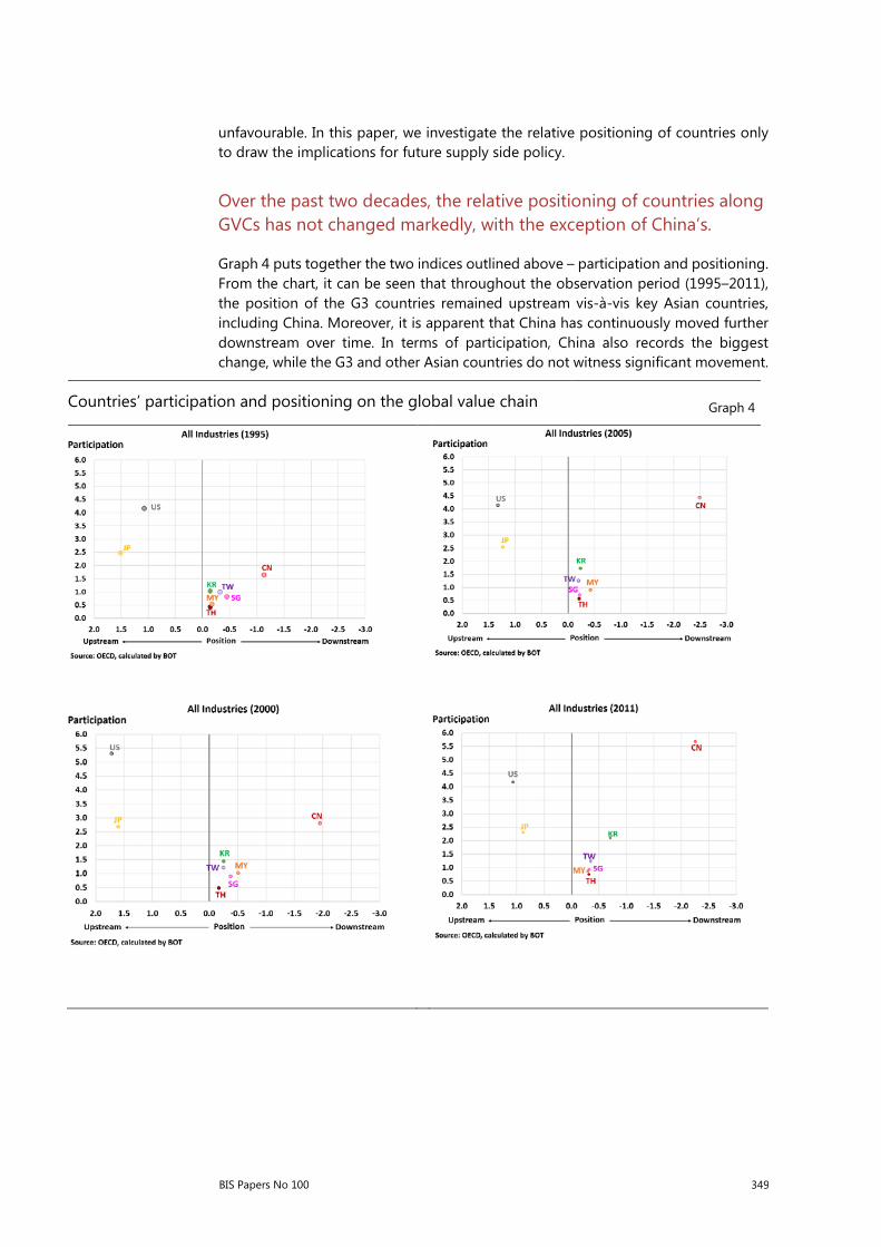
BIS Papers No 100 349
unfavourable. In this paper, we investigate the relative positioning of countries only to draw the implications for future supply side policy.
Over the past two decades, the relative positioning of countries along GVCs has not changed markedly, with the exception of China’s.
Graph 4 puts together the two indices outlined above – participation and positioning. From the chart, it can be seen that throughout the observation period (1995–2011), the position of the G3 countries remained upstream vis-à-vis key Asian countries, including China. Moreover, it is apparent that China has continuously moved further downstream over time. In terms of participation, China also records the biggest change, while the G3 and other Asian countries do not witness significant movement.
Countries’ participation and positioning on the global value chain Graph 4

350 BIS Papers No 100
Part II: Thailand’s experience within GVCs
Although the overall participation index of countries in Asia ex-China has not changed substantially, the nature of participation, ie the level of backward and forward participation, may have changed over time. Moreover, this characteristic may vary from sector to sector. We investigate these issues below.
In Thailand’s case, the degree of downstream positioning is driven by almost all industrial sectors. Over time, the increase in the degree of that positioning has been caused by increasing backward participation rather than falling forward participation.
As seen from Graph 5, most manufacturing sectors in Thailand are positioned downstream, as backward linkages are relatively higher than forward ones. Agriculture, as expected, falls on the upstream side, as agricultural products have a relatively low import content. At the same time, they can be exported in raw form to be used in various agro-manufacturing chains globally. Over time, most sectors have remained more or less in the same position that they occupied two decades ago. In the case of petroleum, which is an exception, we find that the marked shift in positioning from upstream to downstream followed the government’s removal of conditions that discouraged foreign companies from pursuing refinery projects in Thailand. As a result, in the span of just a few years after 1990, domestic refinery capacity almost tripled, while imports of refined products fell proportionately.
In view of each sector’s width and breadth, it is impossible to cover all sectors in this short paper. As a case study, we investigate the electronics and electrical appliances sector, as this sector seems to be more prominent in the global production network than other sectors are. As Graph 6 shows, the sector accounts for a larger share of total foreign value added than do the other sectors. The same applies to
Evolution of Thailand’s key manufacturing sectors in GVCs Graph 5

BIS Papers No 100 351
Thailand. In 2011, electronics and electrical appliances combined represent around 22% of the total foreign value added that the country receives from abroad (Graph 6, right-hand table).
Foreign value added Graph 6
Source: OECD, BOT calculations.
Thailand’s electronics sector generates a lower share of domestic value added to exports than do those of more industrialised Asian peers.
From Graph 7, it can be seen that Thailand’s electronic products sector accounts for a lower share of domestic value added (DVA) than do its North Asian counterparts in Korea and Chinese Taipei, for example. The right-hand chart also shows that Thailand’s DVA has been stagnant over time, at around 40% of total value added generated in the production process. Moreover, firm interviews indicate that the majority of such DVA is generated through labour employment, mostly on the assembly line, rather than through domestic technological know-how. As seen from Graph 8, employment in this industry has grown faster than in the overall manufacturing sector since the early 2000s.
Nevertheless, recent research by the Bank of Thailand (Leepipatpiboon and Thongsri (2018)) indicates that, among all industrial sectors, employment in the electronics sector is most at risk from automation technology. During the past four years, Thailand has witnessed strong growth in electronics production. However, electronic firms have reported increasing purchases of robots that correspond to falling hours of employment (Graph 9). Recent firm visits and internal studies also indicate that a similar pattern has started to emerge in the automotive, rubber, and plastics sectors – which together represent almost a third of Thailand’s industrial output. In this light, the benefit in terms of job creation that Thailand receives from its backward participation in GVCs is likely to diminish further.

352 BIS Papers No 100
Part III: Conclusion
While trade statistics help us measure the impact of GVCs on GDP, the TiVA approach used in this paper allows us to visualise where a country is positioned along the value chain – a more meaningful input when formulating industrial policy. In Thailand’s case, we find that most manufacturing sectors lie toward the downstream end of the chain. Thus, export figures are likely to be large, even on a net basis. In
Domestic value added of selected countries, in E&E sector Graph 7
Employed persons in Thailand Graph 8 Automation in the manufacturing sector
(Index 2001 = 100) Graph 9
Source: Thai Labor Force Survey. Source: National Statistical Office of Thailand, Office of Industrial Economics (Thailand); International Federation of Robotics 2017.

BIS Papers No 100 353
other words, the so-called double-counting problem tends to punish countries which are positioned downstream more heavily than it does those with upstream positioning. As witnessed in recent years, a growing bilateral trade surplus has put upward pressure on the domestic currency, which has been an ongoing concern for Thailand on the external front.
On the domestic front, one obvious concern relates to the nature of backward participation in Thailand. As documented by several research studies, one of the key benefits from backward participation is job creation. In future, however, production processes are likely to become increasingly automated, not least in the electronics sector, where labour-replacement automation is already present on a significant scale. As such disruptive technology penetrates into more sectors, the conventional benefit from job creation is likely to diminish over time.
Looking ahead, policymakers should therefore induce local players to reap benefits from backward participation that are more sustainable, particularly in terms of technological know-how, in order to raise the share of DVA in exports. In fact, government policy is already moving in this direction, under the banner of the “Thailand 4.0” programme. In particular, the Board of Investment – the official body responsible for promoting investment in Thailand – has recently revised its investment promotion schemes to offer extra incentives for firms that adopt advanced technologies or belong to the targeted industries which it deems critical in upgrading the country’s manufacturing sector. In line with the findings of this paper, this marks an important shift in policy orientation away from creating employment and utilisation of raw materials, and towards developing the absorptive capacity of domestic players. Indeed, this is a prerequisite if Thailand is to avoid a two-speed economy where the external sector flourishes while the domestic sector withers.
References
Ahmed, S, M Appendino and M Ruta (2015): “Depreciations without exports? Global value chains and the exchange rate elasticity of exports”, World Bank Policy Research Working Papers, no WPS 7390, Washington DC.
Blalock, G and S Gertler (2007): “Welfare gains from foreign direct investment”, Journal of International Economics, vol 74, no 2, pp 402–21.
Gereffi, G (2015): “Global value chains, development and emerging economies”, Inclusive and Sustainable Industrial Development Working Paper Series, WP 18, United Nations Industrial Development Organization.
Koopman, R, W Powers, Z Wang and S-J Wei (2010): “Give credit where credit is due: tracing value added in global production chains”, NBER Working Papers, no 16426.
Kuroiwa, I (2017): “The automotive value chain in Thailand”, ERIA Discussion Paper Series, DP-2016-33, Economic Research Institute for ASEAN and East Asia.
Leepipatpiboon, P and N Thongsri (2018): “Automation in Thailand and its effects on labor market”, Bank of Thailand, January, www.bot.or.th.
Lopez Gonzalez, J, P Kowalski and P Achard (2015): “Trade, global value chains and wage-income inequality”, OECD Trade Policy Papers, no 182, OECD Publishing, Paris.

354 BIS Papers No 100
World Economic Forum (2012): “The shifting geography of global value chains: implications for developing countries and trade policy”, Global Agenda Council on the Global Trade System.

BIS Papers No 100 355
Globalisation and deglobalisation
Central Bank of the Republic of Turkey
Abstract
Globalisation has contributed positively to the global economy in terms of economic growth and welfare. However, especially amid rising global interdependence, closer synchronisation of business and financial cycles and stronger linkages across monetary, macroprudential and fiscal policies, as well as burgeoning protectionist sentiments, the changes it causes in the flow of goods, services, capital and people can also be disruptive, destabilising processes of production and funding. Future policies should aim to maintain stability while ensuring that efficient flows can be maintained.
Keywords: policy linkages, business cycles, financial cycles, capital movements, goods and services trade, migration, spillovers, emerging markets.
JEL classification: F10, F21, F22, F60, E3, E63.

356 BIS Papers No 100
Introduction
Globalisation contributes to economic growth through increased access to a larger pool of goods and services, financial saving and investment opportunities, flows of workers, the spread of technological progress and improved welfare. Following reforms in the early 1980s, Turkey increased its participation in the global economy by liberalising its trade regime followed by its financial sector and capital accounts. As a result, Turkey today has a globally integrated economy, the 15th largest in the world.
While capital is highly mobile, and trade in goods and services is ever more global, protectionist sentiments are starting to burgeon, especially in the advanced economies. As a result, the mobility of people, another factor of production, is facing even more constraints than before. Despite rising conservative attitudes elsewhere, we in Turkey see this as an opportunity to access a young and dynamic population that is eager to learn and contribute to our future growth prospects.
Increased globalisation has also resulted in a higher synchronisation of business and financial cycles, which calls for the need for greater policy cooperation both internally between monetary policy, fiscal policy and macroprudential policies, as well as internationally. Following the Great Financial Crisis (GFC), the Turkish financial sector has been able to swiftly substitute sources of external funding in response to changes in global liquidity, and is one of the many EMEs that extensively use macroprudential policies.
In sum, globalisation has positive contributions to make in terms of economic growth and welfare. However, especially in a new world setting of increased interdependence, the changes it causes in the flow of goods, services, capital, and people can also be disruptive in nature, destabilising production and funding processes. Future policies should aim to maintain stability while ensuring efficient flows can be maintained.
Capital
Following the liberalisation process that started in the 1980s, Turkey is well integrated into global capital markets and attracts cross-border investments and flows of funds into its domestic markets. Liberalisation efforts in this period were coupled with simultaneous financial innovation and technological progress globally, resulting in lower transaction costs and better payments systems, paving the way for faster, cheaper and more secure transactions, which further augmented the growth of cross-border flows.
Higher level of globalization in financial markets is championed for increasing saving and investment opportunities for both individuals and firms, and raising welfare for market participants through expanded possibilities for diversification. After the onset of the GFC, however, many countries started to discuss the relationship between heightened global integration and increased vulnerability to shocks from abroad. Market participants are concerned about contagion and the spillover of unstable external factors into their domestic financial markets, disrupting markets and causing an inefficient allocation of resources. In this setting, continued

BIS Papers No 100 357
access to foreign sources of funds becomes a concern of utmost importance to most EMEs.
Here Turkey stands out from the rest of its peers, as recent experience has shown that sources of liquidity can be substituted when there is a shortage in one particular region or resource. In addition to the risks raised by the GFC, recently certain regional risks to the traditional sources of global liquidity have increased. A large concentration of funding sourced from one particular region could therefore create a systemically significant potential for disruption if regionally specific risks were to increase. Thanks to their strong fundamentals, Turkish banks have shown resilience against a potential funding concentration risk by increasing their access to sources of liquidity from regions outside the traditional financial centres located in the euro zone, the United Kingdom and the United States.1 As a result, the number of lender countries has increased from around 75 during the time of the crisis to about 110 at the beginning of 2017. The share claimed by the top 10 sources of funding has fallen from 85% to just below 70% in the same period, showing that the diversification consists not only in the number of countries, but also in the volume of funding accessed from the top sources. In the end, the share of non-traditional sources in total external debt has increased from about 15% to 35%.
Currency movements in an environment of high interest rates and financial fluctuations may add to existing macroeconomic risks, especially for countries whose corporate sectors have incurred foreign currency-denominated debt. Compared to peer countries, the ratio of corporate financial debt-to-GDP in the Turkish corporate sector is at relatively moderate levels, and the pace of growth has slowed down in the past two years. While the high rollover rates and long maturity of corporate indebtedness help alleviate concerns over currency and liquidity risks, the currency composition of debt remains a potential concern, as the corporate sector has large FX loans, partly unhedged.
To this end, the CBRT, in coordination with other public entities, has initiated a coordinated study aimed at enhancing price and financial stability and improving the economy’s resilience against FX volatility. As a first step, the Bank has collected granular data on firms to better assess corporate FX positions, cash flows and hedging behaviour. Following this assessment, the roadmap for a possible regulatory framework and a policy response for FX risk management and hedging instruments will be determined in line with the best market practices. Proactive regulation of this nature will certainly contribute not only to financial stability but to overall economic resilience.
Spillovers and policy responses: Another concern raised over the effects of globalization is that heightened global interconnectedness has increased the synchronisation of both business and financial cycles, especially during downturns. In response, many countries have used macroprudential policies in efforts to counter transmission mechanisms and decouple the domestic cycles from the negative cycles seen in external markets. Following an overhaul of the banking sector in 2001, and active use of a wide variety of policies at different points in the cycle in response to varying needs of the market recently, Turkey weathered the GFC and its aftermath relatively well, showing that global integration does not necessarily translate into cycles of equal magnitudes across connected markets. The post-GFC monetary policy stance of advanced economies increased global liquidity and short-term capital flows
1 T Çapacıoğlu (2017).

358 BIS Papers No 100
into EMEs, raising concerns about financial stability risks. Like many other EMEs, Turkey used macroprudential policies to limit fast credit growth. Turkey in particular approached the issue in a multi-faceted manner, and employed a number of measures that limited credit demand and credit supply by applying reserve requirements, general provisions, capital adequacy risk weights, and restrictions on consumer and commercial credit (Graph 1). In response to large fluctuations in some foreign currencies, households were prohibited from taking out FX-based or FX-linked loans, as they have no natural hedge against exchange rate movements. For the same reason, only firms with natural hedges, or large firms above a certain threshold, were allowed to continue borrowing in FX.
Not surprisingly, one of the initial post-crisis measures was loan-to-value (LTV) caps of 75% for retail housing loans and 50% for corporate real estate loans, which were introduced in 2011. A ladder system for LTV caps on vehicle loans was introduced later, which also helped to soften demand for credit and ease the pressure on the currency and current accounts. On the consumer side, further measures to curb demand were taken: as individuals were using credit cards with large number of payment instalments, credit cards were functioning as a short-term credit mechanism rather than a means of payment. To counter this, a cap of nine months on the number of credit card instalments was introduced, credit card minimum payments were tied to credit card limits, and limits were linked to income. The maximum maturity allowed on general purpose loans was restricted to 36 months, and on vehicle loans to 48 months. Non-bank financing companies were also included in the reserve requirement system. The measures were successful in curbing credit growth in the aftermath of the GFC.
More recently, signs of economic recovery in advanced economies have helped slow capital flows into EMEs. Turkey’s credit growth rate has slowed, which was also in part due to the success of the macroprudential policies. In 2016, in a setting of slowing down credit growth in both commercial and retail side, a number of easing measures were implemented. On the consumer side, the LTV ratio for housing loans was increased, the maximum maturity of general purpose loans was increased from
Credit growth and macroprudential policies
(Percent) Graph 1
Note: NPL is drawn scaled to the right-hand axis. Data are from the BRSA, latest data from August 2017.
0
1
2
3
4
5
6
-15
0
15
30
45
60
75
90
105
120
01.0
605
.06
09.0
601
.07
05.0
709
.07
01.0
805
.08
09.0
801
.09
05.0
909
.09
01.1
005
.10
09.1
001
.11
05.1
109
.11
01.1
205
.12
09.1
201
.13
05.1
309
.13
01.1
405
.14
09.1
401
.15
05.1
509
.15
01.1
605
.16
09.1
601
.17
05.1
7
Credit Growth
Retail Credit G.
CC Balance
NPL (Right Axis)
CC Risk Weights
LTV
CC, Provis., RiskW-I
CC, Provis., RiskW-II
Term Limits
Vehicle LTV, CC
CC Installment II
CC Installment I
CC Inst. And Credit
LTV, Term and Inst.

BIS Papers No 100 359
36 months to 48, the number of payment instalments allowed on credit cards was increased from nine to 12, and a restructuring facility for existing balances in credit cards and general purpose loans was implemented with maturities as high as 72 months.2 On the supply side, general provisions for commercial loans were reduced, and the incremental provisioning applied to consumer loans was abolished. As a result, credit growth started to pick up again in the fourth quarter of 2016.
Another outcome of this period was the decoupling of the relationship between credit growth and the NPL rates seen in the economy. NPL rates usually rise as credit growth slows, as seen in the case of the Turkish economy during the GFC. However, following the introduction of macroprudential policies, in the post-2011 era we see that the relationship is much more gradual, with moderate changes in NPL ratio in response to the general slow-down in credit growth.
Migration
As mentioned above, and in parallel with rising protectionist sentiment relating to trade in goods and services, the movement of people – seen as a factor of production that has historically not enjoyed the same level of mobility as capital – has come under even greater scrutiny than before. In Turkey, we have approached the subject of migration first and foremost as a humanitarian matter. While migration does raise various predicaments relating to social adjustment, infrastructural capacity and economic costs; we see the presence of migrants in Turkey as a welcome development that will undoubtedly invigorate the labour market and contribute to our existing multicultural richness.
In a recent paper, CBRT researchers have found the effects of the inflow of Syrian refugees on the local labour force to have been limited, with rather favourable effects on the informal labour sector while having no significantly depressive effect on the wages of local labourers.3 On the other hand, the influx of job seekers has added to the unemployment rate, especially among women and low-skilled workers as well as the informally employed whom they have replaced. The population of migrants has also contributed positively to domestic demand and therefore to GDP growth by some 0.2–0.3 percentage points while the substitution of local informal workers with migrants is calculated to have depressive effect of around 2.5 percentages on CPI.4 And to tie the issue with mobility of capital, there has been an increase in the number of enterprises operating with Syrian capital, which have further contributed to the growth in domestic economic activity.
Further, migrants may elect to return to their countries of origin in the future. But even if they did decide to stay, it would not be accurate to evaluate their presence in the labour market as an inflow of permanently less-skilled labourers. Most migrants are young. Together with future generations, they will have an easier time integrating into society and are expected to be more flexible in closing any skills gap. A similar kind of movement was seen among the Turkish guest labourers in Germany, who started migrating there in the early 1960s. The influx of low skilled-workers, who were
2 S Baziki (2017).
3 Ceritoğlu et al (2017).
4 Konuk and Tümen (2016).

360 BIS Papers No 100
thought to be temporary, proved to be rather permanent. Currently the third generation of migrants has moved up the production ladder, and became an indispensable part of society and the economy, as well as the political sphere with their presence in academia, the sciences, the arts, and representation in both local and federal level politics.
Ultimately we think this issue is best approached with a long-term humane outlook rather than a focus on the short-term economic costs. And if the Turkish migrant experience in Germany is any indication, then we expect the migrant population to contribute to our economic growth and welfare in the long run, which will outweigh any short-term costs.
Goods and services trade
The economic reforms integrating the Turkish economy with global trade began in the early 1980s in the form of growth policies geared towards promoting exports, similar to the experience of many other EMEs. Today, Turkey is well integrated into global trade in goods and services as a liberalised open economy. As the world’s 15th largest economy and the 28th largest export economy, Turkey is a not only an affiliate of multilateral trade agreements through its membership in the European Customs Union, World Trade Organisation and EFTA but it is also a partner in many bilateral trade agreements.5 The EU is Turkey’s largest trading partner in both imports and exports, while Turkey itself ranks fourth among the EU’s export destinations and fifth among its sources of imports.
Turkish exports have moved away from agricultural goods to mostly value added exports, such as machinery, textiles, transport materials, and manufactured goods and metal products.6 A study of export destinations shows that Turkey is well integrated into global markets, selling goods to both EMEs and advanced economies.7 Turkey also benefits from access to other EMEs and advanced economies as sources of intermediate goods.8 This outcome is further supported by the establishment of subsidiaries and other direct investments of foreign firms. China, Russia, Korea and Iran are among the top five sources of intermediate goods, after the EU, and provide the economy with access to machinery and its intermediates, semi-processed metals, plastic goods and resources.
Increased globalisation has seen the development of a more complex bundle of Turkish exports. Productivity fuels economic growth, and a more productive and competitive business environment will yield to a larger global presence through a higher share of global trade. In this regard, it is of utmost importance to analyse the
5 Bilateral trade agreements were signed with Albania, Bosnia-Herzegovina, Chile, Croatia, Egypt,
Georgia, Israel, Jordan, Lebanon, the Republic of Macedonia, Montenegro, Morocco, the Palestinian Authority, Syria, Serbia and Tunisia.
6 Aydın et al (2007) find that the 2001–04 period saw an upward trend in specialisation in high technology-intensive exports compared with the previous six years.
7 The top five export destinations reveal a similar picture: the EU, the United States, Switzerland, Iran and Iraq.
8 Yükseler and Türkan (2006) find that the Turkish export sector is increasingly integrated with imports.

BIS Papers No 100 361
country’s export mix to assess how its firms fare in terms of global competition. In a global study of economic complexity, researchers measure the relative concentration and intensity of knowledge in a country by looking at the range of exported goods.9 Using this measure Turkey’s level of diversity in complex products has placed it as the 40th most complex exporting country in 2015, up from a ranking of 50th in 2000, well above its other EME peers. This indicator has been shown to be a powerful indicator for future growth and shows potential for Turkey to positively diverge from the rest of its peers in the future.10 Turkey has also outperformed its potential in terms of economic size and product range in global comparative advantage: in the latest data available for 2015, Turkey had a global comparative advantage in about 400 products.11
The distributional effects of trade are much discussed both in academia and by policymakers. Trade liberalisation in the 1980s is often championed for having raised per capita incomes in that period. However, the process has also contributed to a widening of the skills gap in many comparable economies. A related question is whether a country’s export composition has influenced its income inequality or if product diversification has been beneficial for various groups within the country. In a study that links the export bundle of countries to the potential level of income inequality relating to products in the export bundle, Turkey’s largest trade volumes are concentrated in the medium range of inequality relating to products.12 Finally, the concentration of firms in the economy shows that the Herfindahl index for the secondary sector is down from an already low score of 0.1 in the early 1992s to about 0.05 at the end of 2016.13 The market share of firms in the top decile also reflects the positive effects of competition and the enlargement of the market base, as the share declined from around 0.45 in the early 1990s to less than 0.3 at end-2016.
Conclusion
Globalisation has made a positive contribution in terms of economic growth and welfare. However, especially in a setting of increased global interdependence, the changes it causes in the flow of goods, services, capital and people can also be disruptive, destabilising processes of production and funding. Future policies should be coordinated with the aim of maintaining stability while ensuring that efficient flows can be maintained.
9 Simoes and Hidalgo (2011).
10 Hidalgo and Hausmann (2009).
11 Simoes and Hidalgo (2011).
12 Simoes and Hidalgo, op cit.
13 The calculations use only firms on the Borsa Istanbul that report net sales in their income statements.

362 BIS Papers No 100
References
Aydın F, H Saygılı and M Saygılı (2007): “Empirical analysis of structural change in Turkish exports”, CBRT Research and Monetary Policy Department, Working Papers, no 07/08.
Baziki, S (2017): “Impact of macroprudential policies on credit use”, CBRT blog post, September.
Çapacıoğlu, T (2017): “More countries, less risk: the changing regional distribution of cross-border bank loans”, CBRT blog post, September.
Ceritoglu E, H Gurcihan Yunculer, H Torun and S Tümen (2017): “The impact of Syrian refugees on natives' labor market outcomes in Turkey: evidence from a quasi-experimental design”, IZA Journal of Labor Policy, vol 6, no 5.
Hidalgo C and R Hausmann (2009): “The building blocks of economic complexity”, Proceedings of the National Academy of Sciences, vol 106, no 26, pp 10570–75.
Konuk, B and S Tümen (2016): “Immigration and prices: quasi-experimental evidence from Syrian refugees”, Journal of Population Economics, vol 29, no 3, pp 657–86.
Simoes A and C Hidalgo (2011): “The economic complexity observatory: an analytical tool for understanding the dynamics of economic development”, workshops at the Twenty-Fifth AAAI Conference on Artificial Intelligence. The Observatory of Economic Complexity Website accessed on 06.10.2017.
Yükseler, Z and E Türkan (2006): “Türkiye’nin Üretim ve DışTicaret Yapısında Yapısal Dönüşüm: Küresel Yönelimler ve Yansımalar”, Ekonomik Araştırmalar Formu Çalışma Raporları Serisi, TÜSİAD-Koç Üniversitesi.
BIS Papers No 100 363
List of participants
Central Banks
Bank of Algeria Ammar Hiouani Deputy Governor Central Bank of Argentina Enrique Szewach Member of the Board Central Bank of Brazil Leonardo Martins Nogueira Head of Governor’s office Central Bank of Chile Joaquín Vial Member of the Board People's Bank of China Dingxin Gao
Chief Representative, Frankfurt Representative Office
Bank of the Republic, Colombia Hernando Vargas Herrera Deputy Governor Czech National Bank Mojmír Hampl
Vice Governor and Member of the Board
Hong Kong Monetary Authority Lillian Cheung Executive Director (Research) Magyar Nemzeti Bank Márton Nagy Deputy Governor Bank Indonesia Dody Budi Waluyo Assistant Governor Bank of Israel Nadine Baudot-Trajtenberg Deputy Governor Bank of Korea Seung-Cheol Jeon Deputy Governor Central Bank of Malaysia Abdul Rasheed Ghaffour Deputy Governor Bank of Mexico Santiago García-Verdú Senior Adviser Central Reserve Bank of Peru Renzo Rossini Miñán General Manager Bangko Sentral ng Pilipinas Diwa Guinigundo Deputy Governor

364 BIS Papers No 100
Narodowy Bank Polski Anna Renata Trzecińska Vice President Saudi Arabian Monetary Authority Fahad Ibrahim AlShathri
Deputy Governor for Research and International Affairs
Monetary Authority of Singapore Keen Meng Choy
Executive Director of Economic Analysis
South African Reserve Bank Daniel Mminele Deputy Governor Bank of Thailand Chantavarn Sucharitakul Assistant Governor Central Bank of the Republic of Turkey Emrah Şener Deputy Governor
Bank for International Settlements
Claudio Borio Head of Monetary and Economic Department
Hyun Song Shin
Economic Adviser and Head of Research
Christian Upper Head of Emerging Markets
BIS Papers No 100 365
Previous volumes from Deputy Governors’ Meetings
No Title Issue date
BIS Papers No 94 Macroprudential frameworks, implementation and relationship with other policies (2017 meeting)
December 2017
BIS Papers No 89 Inflation mechanisms, expectations and monetary policy (2016 meeting)
November 2016
BIS Papers No 83 What do new forms of finance mean for EM central banks? (2015 meeting)
November 2015
BIS Papers No 78 The transmission of unconventional monetary policy to the emerging markets (2014 meeting)
August 2014
BIS Papers No 73 Market volatility and foreign exchange intervention in EMEs: what has changed? (2013 meeting)
October 2013
BIS Papers No 67 Fiscal policy, public debt and monetary policy in emerging market economies (2012 meeting)
October 2012
BIS Papers No 57 The influence of external factors on monetary policy frameworks and operations (2011 meeting)
September 2011
BIS Papers No 54 The global crisis and financial intermediation in emerging market economies (2010 meeting)
December 2010
BIS Papers No 49 Monetary policy and the measurement of inflation: prices, wages and expectations (2009 meeting)
December 2009
BIS Papers No 44 Financial globalisation and emerging market capital flows (2008 meeting)
December 2008
BIS Papers No 35 Transmission mechanisms for monetary policy in emerging market economies (2006 meeting)
January 2008
BIS Papers No 28 The banking system in emerging economies: how much progress has been made? (2005 meeting)
August 2006
BIS Papers No 24 Foreign exchange market intervention: motives, techniques and implications in emerging markets (2004 meeting)
May 2005
BIS Papers No 23 Globalisation and monetary policy in emerging markets (2003 meeting)
May 2005
All volumes are available on the BIS website (www.bis.org).