gmm vs svm for face recognition and face veriﬁcationcdn.intechweb.org/pdfs/17169.pdf · 0 gmm vs...

0

GMM vs SVM for Face Recognitionand Face Verification

Jesus Olivares-Mercado, Gualberto Aguilar-Torres, Karina Toscano-Medina,Mariko Nakano-Miyatake and Hector Perez-Meana

National Polytechnic InstituteMexico

1. Introduction

The security is a theme of active research in which the identification and verification identityof persons is one of the most fundamental aspects nowadays. Face recognition is emerging asone of the most suitable solutions to the demands of recognition of people. Face verificationis a task of active research with many applications from the 80’s. It is perhaps the biometricmethod easier to understand and non-invasive system because for us the face is the most directway to identify people and because the data acquisition method consist basically on to take apicture. Doing this recognition method be very popular among most of the biometric systemsusers. Several face recognition algorithms have been proposed, which achieve recognitionrates higher than 90% under desirable’s condition (Chellapa et al., 2010; Hazem & Mastorakis,2009; Jain et al., 2004; Zhao et al., 2003).The recognition is a very complex task for the human brain without a concrete explanation.We can recognize thousands of faces learned throughout our lives and identify familiar facesat first sight even after several years of separation. For this reason, the Face Recognition isan active field of research which has different applications. There are several reasons for therecent increased interest in face recognition, including rising public concern for security, theneed for identity verification in the digital world and the need for face analysis and modelingtechniques in multimedia data management and computer entertainment. Recent advances inautomated face analysis, pattern recognition, and machine learning have made it possible todevelop automatic face recognition systems to address these applications (Duda et al., 2001).This chapter presents a performance evaluation of two widely used classifiers such asGaussian Mixture Model (GMM) and Support Vector Machine (SVM) for classification taskin a face recognition system, but before beginning to explain about the classification stage itis necessary to explain with detail the different stages that make up a face recognition systemin general, to understand the background before using the classifier, because the stages thatprecede it are very important for the proper operation of any type of classifier.

1.1 Face recognition system

To illustrate the general steps of a face recognition system consider the system shown in Fig.1, which consists of 4 stages:

2

www.intechopen.com

2 Will-be-set-by-IN-TECH

Fig. 1. General Structure of a face recognition system.

1.1.1 Capture

This stage is simple because it only needs a camera to take the face image to be procesed. Dueto this is not necessary to have a camera with special features, currently cell phones have acamera with high resolution which would serve or a conventional camera would be more thanenough because the image can be pre-processed prior to extract the image features. Obviously,if the camera has a better resolution can be obtained clearer images for processing.

1.1.2 Pre-processing

In this stage basically apply some kind of cutting, filtering, or some method of imageprocessing such as normalization, histogram equalization or histogram specification, amongothers. This is to get a better image for processing by eliminating information that is notuseful in the case of cutting or improving the quality of the image as equalization. Thepre-processing of the image is very important because with this is intended to improve thequality of the images making the system more robust for different scenarios such as lightingchanges, possibly noise caused by background, among others.

1.1.3 Feature extraction

The feature extraction stage is one of the most important stages in the recognition systemsbecause at this stage are extracted facial features in correct shape and size to give a goodrepresentation of the characteristic information of the person, that will serve to have a goodtraining of the classification models.Today exists great diversity of feature extraction algorithms, the following are listed some ofthem:

• Fisherfaces (Alvarado et al., 2006).

• Eigenfaces(Alvarado et al., 2006).

• Discrete Walsh Transform (Yoshida et al., 2003).

• Gabor Filters (Olivares et al., 2007).

• Discrete Wavelet Transform (Bai-Ling et al., 2004).

• Eigenphases (Savvides et al., 2004).

1.1.4 Classifiers

The goal of a classifier is to assign a name to a set of data for a particular object or entity. Itdefines a set of training as a set of elements, each being formed by a sequence of data for aspecific object. A classifier is an algorithm to define a model for each class (object specific),so that the class to which it belongs an element can be calculated from the data values thatdefine the object. Therefore, more practical goal for a classifier is to assign of most accurateform to new elements not previously studied a class. Usually also considered a test set thatallows measure the accuracy of the model. The class of each set of test is known and is used tovalidate the model. Currently there are different ways of learning for classifiers among whichare the supervised and unsupervised.

30 Reviews, Refinements and New Ideas in Face Recognition

www.intechopen.com

GMM vs SVM for Face Recognition

and Face Verification 3

In supervised learning, a teacher provides a category label or cost for each pattern in a trainingset, and seeks to reduce the sum of the costs for these patterns. While in unsupervised learningor clustering there is no explicit teacher, and the system forms clusters or “natural groupings”of the input patterns. “Natural”is always defined explicitly or implicitly in the clusteringsystem itself; and given a particular set of patterns or cost function, different clusteringalgorithms lead to different clusters.Also, is necessary to clarify the concept of identification and verification. In identification thesystem does not know who is the person that has captured the characteristics (the human facein this case) by which the system has to say who owns the data just processed. In verificationthe person tells the system which is their identity either by presenting an identification cardor write a password key, the system captures the characteristic of the person (the human facein this case), and processes to create an electronic representation called live model. Finally, theclassifier assumes an approximation of the live model with the reference model of the personwho claimed to be. If the live model exceeds a threshold verifying is successful. If not, theverification is unsuccessful.

1.1.4.1 Classifiers types.

Exist different types of classifiers that can be used for a recognition system in order to chooseone of these classifiers depends on the application for to will be used, it is very important totake in mind the selection of the classifier because this will depend the results of the system.The following describes some of the different types of classifiers exist.

Nearest neighbor. In the nearest-neighbor classification a local decision rule is constructedusing the k data points nearest the estimation point. The k-nearest-neighbors decision ruleclassifies an object based on the class of the k data points nearest to the estimation pointx0. The output is given by the class with the most representative within the k nearestneighbors. Nearness is most commonly measured using the Euclidean distance metric inx-space (Davies E. R., 1997; Vladimir & Filip, 1998).

Bayes’ decision. Bayesian decision theory is a fundamental statistical approach to theproblem of pattern recognition. This approach is based on quantifying the tradeoffsbetween various classification decisions using probability and the costs that accompanysuch decisions. It makes the assumption that the decision problem is posed in probabilisticterms, and that all of the relevant probability values are known (Duda et al., 2001).

Neural Networks. Artificial neural networks are an attempt at modeling the informationprocessing capabilities of nervous systems. Some parameters modify the capabilities ofthe network and it is our task to find the best combination for the solution of a givenproblem. The adjustment of the parameters will be done through a learning algorithm, i.e.,not through explicit programming but through an automatic adaptive method (Rojas R.,1996).

Gaussian Mixture Model. A Gaussian Mixture Model (GMM) is a parametric probabilitydensity function represented as a weighted sum of Gaussian component densities.GMMs are commonly used as a parametric model of the probability distribution ofcontinuous measurements or features in a biometric system, such as vocal-tract relatedspectral features in a speaker recognition system. GMM parameters are estimated fromtraining data using the iterative Expectation-Maximization (EM) algorithm or MaximumA Posteriori MAP) estimation from a well-trained prior model (Reynolds D. A., 2008).

Support Vector Machine. The Support Vector Machine (SVM) is a universal constructivelearning procedure based on the statistical learning theory. The term “universal”means

31GMM vs SVM for Face Recognition and Face Verification

www.intechopen.com


that the SVM can be used to learn a variety of representations, such as neural net (withthe usual sigmoid activation), radial basis function, splines, and polynomial estimators. Inmore general sense the SVM provides a new form of parameterization of functions, andhence it can be applied outside predictive learning as well (Vladimir & Filip, 1998).

In This chapter presents only two classifiers, the Gaussian Mixture Model (GMM) and SupportVector Machine (SVM) as it classifiers are two of the most frequently used on different patternrecognition systems, and then a detailed explanation and evaluation of the operation of theseclassifier is required.

2. Gaussian Mixture Model

2.1 Introduction.

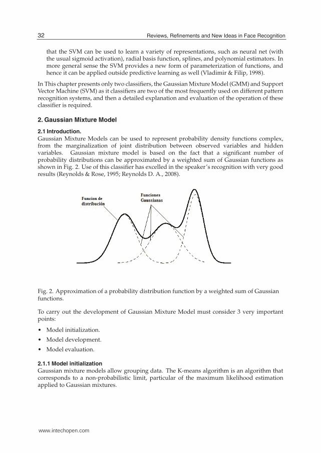
Gaussian Mixture Models can be used to represent probability density functions complex,from the marginalization of joint distribution between observed variables and hiddenvariables. Gaussian mixture model is based on the fact that a significant number ofprobability distributions can be approximated by a weighted sum of Gaussian functions asshown in Fig. 2. Use of this classifier has excelled in the speaker’s recognition with very goodresults (Reynolds & Rose, 1995; Reynolds D. A., 2008).

Fig. 2. Approximation of a probability distribution function by a weighted sum of Gaussianfunctions.

To carry out the development of Gaussian Mixture Model must consider 3 very importantpoints:

• Model initialization.

• Model development.

• Model evaluation.

2.1.1 Model initialization

Gaussian mixture models allow grouping data. The K-means algorithm is an algorithm thatcorresponds to a non-probabilistic limit, particular of the maximum likelihood estimationapplied to Gaussian mixtures.


www.intechopen.com



The problem is to identify data groups in a multidimensional space. It involves a set x1..., xN

of a random variable of D-dimensions in a Euclidean space. A group can be thought of as adata set whose distance between them is small compared to the distance to points outside thegroup.Introducing a set of D-dimensional vectors µk, with k = 1, 2, . . . , K where µk is the prototypeassociated with the k-th group. The goal is to find an assignment of the observed data to thegroups, as well as a set of vectors µk as to minimize the sum of the squares of the distancesbetween each point to its nearest vector µk.For example, initially select the first M feature vectors as the initial centers, as shown in Figure3, ie:

µi = Xi (1)

Fig. 3. Illustration of K-Means algorithm for M3.

Then is added a vector more and get the distance between the new vector and M centers,determining that the new vector belongs to the center with which the distance is the lowest.Subsequently the new center is calculated by averaging the items belonging to the center.Thus denoting by Xi,j the characteristic vectors belonging to the center µ − k, the new centeris given by:

µk =1

N

N

∑j=1

Xk,j (2)

This process is repeated until the distance between the k − th center on the iteration n andn + 1 is less than a given constant.Figure 3 shows that the first three vectors are used as initial centers. Then insert the fourthvector which has the shortest distance from the center x. Subsequently the new center is


www.intechopen.com


calculated by averaging the two vectors belonging to the center X. Then is analyzed the vector5, which has a shorter distance from the center O, which is modified by using the vectors 1and 5, as shown in the second iteration in Figure 3. Then is analyzed the vector 6, which hasa minimum distance to the center O. Here the new center O vectors are modified using 1, 5and 6. The process continues until ninth iteration, where the center O is calculated using thevectors 1, 5, 6, 9, 12; the center X is calculated using the vector 2, 4, 8, 11, while the Y is obtained3, 7, 10 from the vectors.After obtaining the centers, the variance of each center is obtained using the relationship:

σk =1

N

Nk

∑j=1

(µk − Xk,j

)2(3)

2.1.2 Model development

Gaussian Mixture Models(GMM) are statistical modeling methods while a model is definedas a mixture of a certain numbers of Gaussian functions for the feature vectors (Jin et al., 2004).A Gaussian mixture density is a weighted sum of M component densities , this is shown inFigure 4 and obtained by the following equation:

p(x|λ) =M

∑i=1

pibi(x) (4)

Where x is a N-dimensional vector, bi(−→x ),i = 1, 2, . . . , M, are the components of density and

pi , i = 1, 2, . . . , M, are weights of the mixtures. Each component density is a D-Gaussianvariation of the form:

bi(−→x ) =

1

(2π)D2 |σi|

12

exp

{−

1

2(x − µi)

′σ−1i (x − µi)

}(5)

Where ()′ denotes the transposed vector, µ − i denotes the average value of N dimensions andσi covariance matrix which is diagonal, and pi the distribution of weights which satisfy therelationship:

M

∑i=1

pi = 1 (6)

So the distribution model is determined by the mean vector, covariance matrix and theweights of the distribution with which the model is represented as:

λ = pi, µi, σi, i = 1, 2, . . . , M (7)

The estimation of system parameters using the ML algorithm (Maximum Likeklihood) seeksto find the parameters to approximate the best possible distribution of the characteristics ofthe face under analysis and will seek to find the parameters of λ to maximize distribution. Fora sequence of T training vectors X = x1, . . . , xT, the GMM likelihood can be written as:

p(X|λ) =T

∏t=1

p(Xt|λ) (8)

Unfortunately, Equation 8 is nonlinear in relation to the parameters of λ, so to is possible tomaximize directly, so it must use an iterative algorithm called Baum-Welch. Baum-Welch


www.intechopen.com



Fig. 4. Gaussian Mixture Model, GMM

algorithm is used by HMM algorithm to estimate its parameters and has the same basicprinciple of the algorithm of Expectation Maximization (EM Expectation-Maximization),which is part of an initial set of parameters λ(r − 1) and a new model is estimated λ(r), wherer denotes the r − th iteration, so to:

p(X|λ(r)) ≥ P(X|λ(r − 1)) (9)

Thus, this new model (−→λ ), becomes the initial model for the next iteration. Each T elements

must update the model parameters as follows:

Pesos de la mezcla

pi =1

T

T

∑t=1

p(i|Xt+k, λ) (10)

Media

µi =∑

Tt=1 p(i|Xt+k, λ)Xt+k

∑Tt=1 p(i|Xt+k, λ)

(11)

Covarianza

σi =∑

Tt=1 p(i|Xt+k, λ)(Xt+k − σi)

2

∑Tt=1 p(i|Xt+k, λ)

(12)

To calculate the posterior probability is obtained by:

p(i|Xt+k, λ) =pibi(Xt+k)

∑Mj=1 pjbj(Xt+k)

(13)

2.1.3 Model evaluation

In order to carry out the evaluation of the model considers that the system will be used toidentify R people, which are represented by models λ1, λ2, λ3, . . . , λR. The aim is then to findthe model with maximum posterior probability for a given observation sequence. Formally,the person identified is one that satisfies the relation:


www.intechopen.com


R̂ = arg max Pr(λk|X), k = 1, 2, . . . , R (14)

Using Bayes theorem, equation 14 can be expressed as:

R̂ = arg maxp(X|λk)Pr(λk)

p(X), k = 1, 2, . . . , R (15)

Assuming to the probability of each person is equally likely, then Pr(λk) =1R and taking into

account to P(X) is the same for all models of speakers, equation 15 simplifies to:

R̂ = arg max p(X|λk), k = 1, 2, . . . , R (16)

Replacing p(X|λk),

p(X|λ) =T

∏t=1

p(Xt |λk) (17)

in equation 16 yields:

R̂ = arg maxT

∏t=1

p(Xt |λk), k = 1, 2, . . . , R (18)

Finally using logarithms have:

R̂ = arg maxT

∑t=1

log10(p(Xt |λk)), k = 1, 2, . . . , R (19)

where p(Xt |λk) is given by the equation 4, that is by the output of the system shown in Figure4.

3. Support Vector Machine

The Support Vector Machine (SVM) (Vladimir & Filip, 1998) is a universal constructivelearning procedure based on the statistical learning theory. Unlike conventional statistical andneural network methods, the SVM approach does not attempt to control model complexity bykeeping the number of features small. Instead, with SVM the dimensionality of z-space canbe very large because the model complexity is controlled independently of its dimensionality.The SVM overcomes two problems in its design: The conceptual problem is how to controlthe complexity of the set of approximating functions in a high-dimensional space in orderto provide good generalization ability. This problem is solved by using penalized linearestimators with a large number of basis functions. The computational problem is how toperform numerical optimization in a high-dimensional space. This problem is solved bytaking advantage of the dual kernel representation of linear functions.The SVM combines four distinct concepts:

1. New implementation of the SRM inductive principle. The SVM use a special structure thatkeeps the value of the empirical risk fixed for all approximating functions but minimizesthe confidence interval.

2. Input samples mapped onto a very high-dimensional space using a set of nonlinear basis functionsdefined a priori. It is common in pattern recognition applications to map the input vectorsinto a set of new variables which are selected according to a priori assumptions about the


www.intechopen.com



learning problem. For the support vector machine, complexity is controlled independentlyof the dimensionality of the feature space (z-space).

3. Linear functions with constraints on complexity used to approximate or discriminate the inputsamples in the high-dimensional space. The support vector machine uses a linear estimatorsto perform approximation. As it, nonlinear estimators potentially can provide a morecompact representation of the approximation function; however, they suffer from twoserious drawbacks: lack of complexity measures and lack of optimization approacheswhich provide a globally optimal solution.

4. duality theory of optimization used to make estimation of model parameters in a high-dimensionalfeature space computationally tractable. For the SVM, a quadratic optimization problemmust be solved to determine the parameters of a linear basis function expansion. Forhigh-dimensional feature spaces, the large number of parameters makes this problemintractable. However, in its dual form this problem is practical to solve, since itscales in size with the number of training samples. The linear approximating functioncorresponding to the solution of the dual is given in the kernel representation rather thanin the typical basis function representation. The solution in the kernel representation iswritten as a weighted sum of the support vectors.

3.1 Optimal separating hyperplane

A separating hiperplane is a linear fuction that is capable of separating the training datawithout error (see Fig. 5). Suppose that the training data consisting of n samples

(x1, y1), . . . , (xn , yn), x ∈ ℜd, y ∈ +1,−1 can be separated by the hypoerplane decisionfunction

D(x) = (w · x) + w0 (20)

Fig. 5. Classification (linear separable case)

with appropriate coefficients w and w0. A separating hyperplane satisfies the constraints thatdefine the separation of the data samples:

(w · x) + x0 ≥ +1 if yi = +1

(w · x) + x0 ≤ −1 if yi = −1, i = 1, . . . , n (21)


www.intechopen.com


For a given training data set, all possible separating huperplanes can be represented in theform of equation 21.The minimal distance from the separating hyperplane to the closest data point is called themargin and will denoted by τ. A separating hyperplane is called optimal if the margin isthe maximum size. The distance between the separating hyperplane and a sample x′ is|D(x′)|/||w||, assuming that a margin τ exists, all training patterns obey the inequality:

ykD(xk)

||w||≥ τ, k = 1, . . . , n (22)

where yk ∈ −1, 1.The problem of finding the optimal hyperplane is that of finding the w that maximizes themargin τ. Note that there are an infinite number of solutions that differ onlu in scaling of w.To limit solutions, fix the scale on the product of τ and norm of w,

τ||w|| = 1 (23)

Thus maximizing the margin τ is equivalent to minimizing the norm of w. An optimalseparating hyperplane is one that satisfies condition (21 above and additionally minimizes

η(w) = ||w||2 (24)

with respect to both w and w0. The margin relates directly to the generalization ability of theseparating hyperplane. The data points that exist at margin are called the support vectors (Fig.5). Since the support vectors are data points closest to the decision surface, conceptually theyare the samples that are the most difficult to classify and therefore define the location of thedecision surface.The generalization ability of the optimal separating hyperplane can be directly related to thenumber of support vectors.

En[Errorrate] ≤En[Numbero f supportvectors]

n(25)

The operator En denotes expectation over all training sets of size n. This bound is independentof the dimensionality of the space. Since the hyperplane will be employed to develop thesupport vector machine, its VC-dimension must be determined in order to build a nestedstructure of approximating functions.For the hyperplane functions (21) satisfying the constraint ||w||2 ≤ c, the VC-dimension isbounded by

h ≤ min(r2c, d) + 1 (26)

where r is the radius of the smallest sphere that contains the training input vectors (x1, . . . , xn).The factor r provides a scale in terms of the training data for c. With this measure of theVC-dimension, it is now possible to construct a structure on the set of hyperplanes accordingto increasing complexity by controlling the norm of the weights ||w||2:

Sk = (w · x) + w0 : ||w||2 ≤ ck, c1 < c2 < c3 . . . (27)

The structural risk minimization principle prescribes that the function that minimizes theguaranteed risk should be selected in order to provide good generalization ability.By definition, the separating hyperplane always has zero empirical risk, so the guaranteedrisk is minimized by minimizing the confidence interval. The confidence interval is minimized


www.intechopen.com



by minimizing the VC-dimension h, which according to (26) corresponds to minimizing thenorm of the weights ||w||2. Finding an optimal hyperplane for the separable case is a quadraticoptimization problem with linear constraints, as formally stated next.Determine the w and w0 that minimize the functional

η(w) =1

2||w||2 (28)

subject to the constraints

yi[(w · x) + w0] ≥ 1, i = 1, . . . , n (29)

given the training data (xi, yi), i = 1, . . . , n, x ∈ ℜd. The solution to this problem consistsof d + 1 parameters. For data of moderate dimension d, this problem can be solved usingquadratic programming.For training data that cannot be separated without error, it would be desirable to separatethe data with a minimal number or errors. In the hyperplane formulation, a data point isnonseparable when it does not satisfy equation (21). This corresponds to a data point thatfalls within the margin or on the wrong side of the decision boundary. Positive slack variablesξi, i = 1, . . . , n, can be introdiced to quantify the nonseparable data in the defining conditionof the hyperplane:

yi[(w · x) + w0] ≥ 1 − ξi (30)

For a training sample xi, the slack variable ξi is the deviation from the margin bordercorresponding to the class of yi see Fig. 6. According to our definition, slack variables greaterthan zero correspond to misclassified samples. Therefore the number of nonseparable samplesis

Q(w) =n

∑i=1

I(ξi > 0) (31)

Numerically minimizing this functional is a difficult combinatorial optimization problembecause of the nonlinear indicator function. However, minimizing (31) is equivalent tominimizing the functional

Q(ξ) =n

∑i=1

ξpi (32)

where p is a small positive constant. In general, this minimization problem is NP-complete.To make the problem tractable, p will be set to one.

3.2 Inner product kernel

The inner product kernel (H) is known a priori and used to form a set of approximatingfunctions, this is determined by the sum

H(x, x′) =m

∑j=1

gj(x)gj(x′) (33)

where m may be infinite.Notice that in the form (33), the evaluation of the inner products between the feature vectors ina high-dimensional feature space is done indirectly via the evaluation of the kernel H betweensupport vectors and vectors in the input space. The selection of the type of kernel function


www.intechopen.com


Fig. 6. Nonseparable case

corresponds to the selection of the class of functions used for feature construction. The generalexpression for an inner product in Hilbert space is

(z · z′) = H(x, x′) (34)

where the vectors z and z′ are the image in the m-dimensional feature space and vectors x andx′ are in the input space.Below are several common classes of multivariate approximating functions and their innerproduct kernels:

Polynomials of degree q have inner product kernel

H(x, x′) = [(x · x′) + 1]q (35)

Radial basis functions of the form

f (x) = sign

(n

∑i=1

αi exp

{−|x − xi|

2

σ2

})(36)

where σ defines the width have the inner product kernel

H(x, x′) = exp

{−|x − x′|2

σ2

}(37)

Fourier expansion

f (x) = vo +q

∑j=1

(vj cos(jx) + wj sin(jx)) (38)

has a kernel

H(x, x′) =sin(q + 1

2 )(x − x′)

sin(x − x′)/2(39)


www.intechopen.com



4. Evaluation results

Here are some results with both classifiers, GMM and SVM combined with some featureextraction methods mentioned above, like Gabor, Wavelet and Eigenphases. The resultsshown were performed using the database “The AR Face Database”(Martinez, 1998) is used,which has a total of 9, 360 face images of 120 people (65 men and 55 women) that includes faceimages with several different illuminations, facial expression and partial occluded face imageswith sunglasses and scarf. Two different training set are used, the first one consists on imageswithout occlusion, in which only illumination and expressions variations are included. Onthe other hand the second image set consist of images with and without occlusions, as well asillumination and expressions variations. Here the occlusions are a result of using sunglassesand scarf. These images sets and the remaining images of the AR face database are used fortesting.Tables 1 and 2 shows the recognition performance using the GMM as a classifier. Therecognition performance obtained using the Gabor filters-based, the wavelet transform-basedand eigenphases features extraction methods are shown form comparison. Table 1 showsthat when the training set 1 is used for training, with a GMM as classifier, the identificationperformance decrease in comparison with the performance obtained using the training set2. This is because the training set 1 consists only of images without occlusion and thensystem cannot identify several images with occlusion due to the lack of information aboutthe occlusion effects. However when the training set 2 is used the performance of all of themincrease, because the identification system already have information about the occlusioneffects.

Image set 1 Image set 2Gabor 71.43 % 91.53 %

Wavelet 71.30 % 92.51 %

Eigenphases 60.63 % 87.24 %

Table 1. Recognition using GMM

Image set 1 Image set 2

Average False acceptance False reject False acceptance False rejectGabor 4.74 % 7.26 % 1.98 % 4.13 %

Wavelet 6.69 % 6.64 % 1.92 % 5.25 %

Eigenphases 37.70 % 14.83 % 21.39 % 21.46 %

Table 2. Verification using GMM

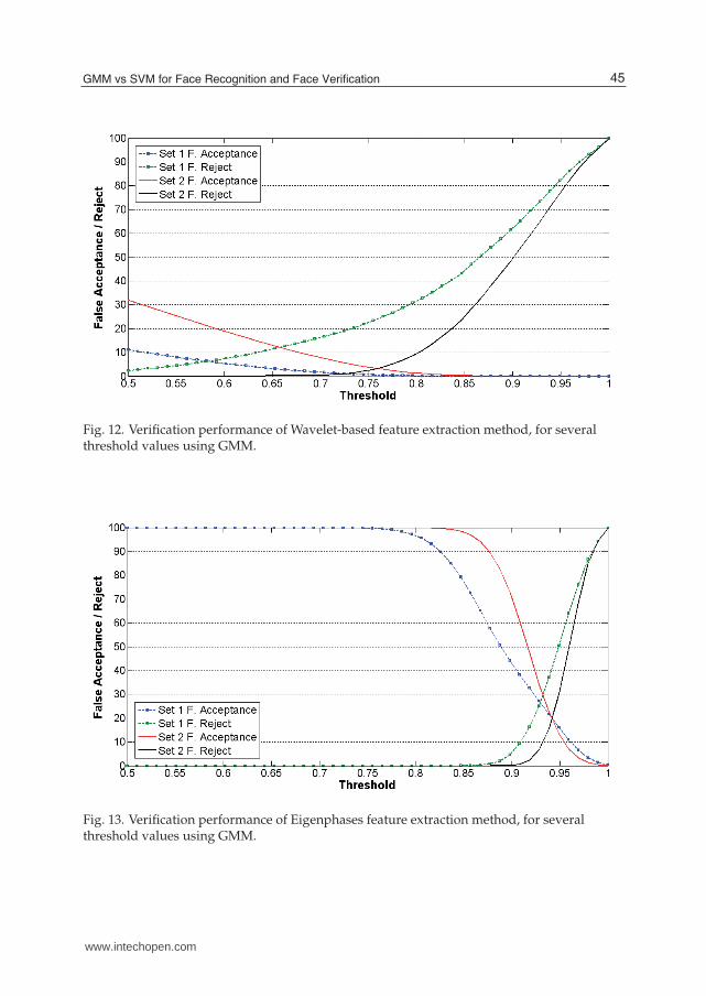
Tables 3 and 4 show the obtained results with Gabor filters, Wavelet and Eigenphases asfeatures extractors methods in combination with SVM for identification and verification task.Also shows the same characteristics like GMM when the training set 1 and training set 2 areused for training.Figs. 7 and 8 shows the ranking performance evaluation of Gabor, Wavelets and eigenphasesfeature extractions methods, using GMM for identitification and Figs. 9 and 10 shows theranking performance evaluation of Gabor, Wavelet and Eigenphases with the Support VectorMachine for identification.In Figs. 11-13 shows the evaluation of the GMM as verifier using different thresholds foracceptance in these graphs shows the performance of both the false acceptance and the falserejection. Showing the moment when both have the same percentage, depending on the needs


www.intechopen.com


Fig. 7. Ranking performance evaluation using GMM and Training set 1.

Fig. 8. Ranking performance evaluation using GMM and Training set 2.


www.intechopen.com



Fig. 9. Ranking performance evaluation using SVM and Training set 1.

Fig. 10. Ranking performance evaluation using SVM and Training set 2.


www.intechopen.com


Image set 1 Image set 2Gabor 75.98 % 94.90 %

Wavelet 79.54 % 97.29 %

Local 3 84.44 % 97.67 %Local 6 81.05 % 97.29 %

Local fourier 3 85.92 % 97.92 %

Local fourier 6 85.59 % 97.85 %Eigenphases 80.63 % 96.28 %

Table 3. Recognition using SVM

Image set 1 Image set 2

Average False acceptance False reject False acceptance False reject

Gabor 0.43 % 22.65 % 0.12 % 8.38 %Wavelet 0.17 % 22.27 % 0.04 % 4.64 %

Eigenphases 0.001 % 34.74 % 0.002 % 16.04 %

Table 4. Verification using SVM

will have to choose a threshold. In Figs. 14-16 shows the evaluation of the SVM as verifierusing also different thresholds.

Fig. 11. Verification performance of Gabor-based feature extraction method, for severalthreshold values using GMM.

5. Conclusion

In this chapter presented two classifiers that can be used for face recognition, and shown someevaluation results where the GMM and SVM are used for identification and verification tasks.Two different image sets were used for training. One contains images with occlusion and the


www.intechopen.com



Fig. 12. Verification performance of Wavelet-based feature extraction method, for severalthreshold values using GMM.

Fig. 13. Verification performance of Eigenphases feature extraction method, for severalthreshold values using GMM.


www.intechopen.com


Fig. 14. Verification performance of Gabor-based feature extraction method, for severalthreshold values using SVM.

Fig. 15. Verification performance of Wavelet-based feature extraction method, for severalthreshold values using SVM.


www.intechopen.com



Fig. 16. Verification performance of Eigenphases feature extraction method, for severalthreshold values using SVM.

other one contains images without occlusions. The performance of this classifiers are shownusing the Gabor-based, Wavelet-based and Eigenphases method for feature extraction.It is important to mention, at the verification task it is very important to keep the falseacceptation rate as low as possible, without much increase of the false rejection rate. To finda compromise between both errors, evaluation results of both errors with different thresholdsare provided. To evaluate the performance of proposed schemes when they are required toperform an identification task the rank(N) evaluation was also estimated.Evaluation results show that, in general, the SVM performs better that the GMM, specially,when the training set is relatively small. This is because the SVM uses a supervised trainingalgorithm and then it requires less training patterns to estimate a good model of the personunder analysis. However it requires to jointly estimating the models of all persons in thedatabase and then when a new person is added, the all previously estimated models must becomputed again. This fact may be an important limitation when the database changes withthe time, as well as, when huge databases must be used, as in banking applications. On theother hand, because the GMM is uses a non-supervised training algorithm, it requires a largernumber of training patterns to achieve a good estimation of the person under analysis andthen its convergence is slower that those of SVM, however the GMM estimated the model ofeach person independently of that of the other persons in the database. It is a very importantfeature when large number of persons must be identified and the number of persons growswith the time because, using the GMM, when a new person is added, only the model of thenew person must be added, remaining unchanged the previously estimated ones. Thus theGMM is suitable for applications when large databases must be handed and they change withthe time, as in banking operations. Thus in summary, the SVM is more suitable when the sizeof databases under analysis is almost constant and it is not so large, while the GMM is moresuitable for applications in which the databases size is large and it changes with the time.


www.intechopen.com


6. References

Alvarado G.; Pedrycz W.; Reformat M. & Kwak K. C. (2006). Deterioration of visualinformation in face classification using Eigenfaces and Fisherfaces. Machine Visionand Applications, Vol. 17, No. 1, April 2006, pp. 68-82, ISSN: 0932-8092.

Bai-Ling Z.; Haihong Z. & Shuzhi S. G. (2004). Face recognition by applying wavelet subbandrepresentation and kernel associative memory. Neural Networks, IEEE Transactions on,Vol. 15, Issue:1, January. 2004, pp. 166 - 177, ISSN: 1045-9227.

Chellapa R.; Sinha P. & Phillips P. J.(2010), Face recognition by computers and humans.Computer Magazine, Vol. 43, Issue 2, february 2010, pp. 46-55, ISSN: 0018-9162.

Davies E. R. (1997). Machine Vision: Theory, Algorithms, Practicalities, Academic Press, ISBN:0-12-206092-X, San Diego, California, USA.

Duda O. R; Hart E. P. & Stork G. D. (2001). Pattern Classification, Wiley-Interscience, ISBN:0-471-05669-3, United States of America.

Hazem. M. El-Bakry & Mastorakis N. (2009). Personal identification through biometrictechnology, AIC’09 Proceedings of the 9th WSEAS international conference on Appliedinformatics and communications, pp. 325-340, ISBN: 978-960-474-107-6, World Scientificand Engineering Academy and Society (WSEAS) Stevens Point, Wisconsin, USA.

Jain, A.K.; Ross, A. & Prabhakar, S. (2004). An introduction to biometric recognition. IEEETrans. on Circuits and Systems for Video Technology, Vol. 14, Jan. 2004, pp. 4-20, ISSN:1051-8215.

Jin Y. K.; Dae Y. K. & Seung Y. N. (2004), Implementation and enhancement of GMMface recognition systems using flatness measure. IEEE Robot and Human InteractiveCommunication, Sept. 2004, pp. 247 - 251, ISBN: 0-7803-8570-5.

Martinez A. M. & Benavente R. (1998). The AR Face Database. CVC Technical Report No. 24,June 1998.

Olivares M. J.; Sanchez P. G.; Nakano M. M. & Perez M. H. (2007). Feature Extraction andFace Verification Using Gabor and Gaussian Mixture Models. MICAI 2007: Advancesin Artificial Intelligence, Gelbukh A. & Kuri M. A., pp. 769-778, Springer Berlin /Heidelberg.

Reynolds D.A. & Rose R.C. (1995). Robust text-independent speaker identification usinggaussian mixture speaker models. IEEE Transactions on Speech and Audio Processing,Vol. 3, Issue 1, Jan. 1995, pp. 72-83, ISSN: 1063-6676.

Reynolds D.A. (2008). Gaussian Mixture Models, Encyclopedia of Biometric Recognition, Springer,Feb 2008, , ISBN 978-0-387-73002-8.

Rojas R. (1995). Neural networks: a systematic introduction, Springer-Verlag, ISBN: 3-540-60505-3,New York.

Savvides, M.; Kumar, B.V.K.V. & Khosla, P.K. (2004). Eigenphases vs eigenfaces. Pro- ceedings ofthe 17th International Conference on Pattern Recognition, Vol. 3, Aug. 2004, pp. 810-813,ISSN: 1051-4651.

Vladimir C. & Filip M. (1998). Learning From Data: Concepts, Theory, and Methods, WileyInter-Science, ISBN: 0-471-15493-8, USA.

Yoshida M.; Kamio T. & Asai H. (2003). Face Image Recognition by 2-DimensionalDiscrete Walsh Transform and Multi-Layer Neural Network, IEICE Transactions onFundamentals of Electronics, Communications and Computer., Vol. E86-A, No. 10, October2003, pp.2623-2627, ISSN: 0916-8508.

Zhao W.; Chellappa R.; Phillips P. J. & RosenfeldA. (2003). Face recognition: A literaturesurvey. ACM Computing Surveys (CSUR), Vol. 35, Issue 4, December 2003, pp. 399-459.


www.intechopen.com

Reviews, Refinements and New Ideas in Face RecognitionEdited by Dr. Peter Corcoran

ISBN 978-953-307-368-2Hard cover, 328 pagesPublisher InTechPublished online 27, July, 2011Published in print edition July, 2011

InTech EuropeUniversity Campus STeP Ri Slavka Krautzeka 83/A 51000 Rijeka, Croatia Phone: +385 (51) 770 447 Fax: +385 (51) 686 166www.intechopen.com

InTech ChinaUnit 405, Office Block, Hotel Equatorial Shanghai No.65, Yan An Road (West), Shanghai, 200040, China

Phone: +86-21-62489820 Fax: +86-21-62489821

As a baby one of our earliest stimuli is that of human faces. We rapidly learn to identify, characterize andeventually distinguish those who are near and dear to us. We accept face recognition later as an everydayability. We realize the complexity of the underlying problem only when we attempt to duplicate this skill in acomputer vision system. This book is arranged around a number of clustered themes covering differentaspects of face recognition. The first section on Statistical Face Models and Classifiers presents reviews andrefinements of some well-known statistical models. The next section presents two articles exploring the use ofInfrared imaging techniques and is followed by few articles devoted to refinements of classical methods. Newapproaches to improve the robustness of face analysis techniques are followed by two articles dealing withreal-time challenges in video sequences. A final article explores human perceptual issues of face recognition.

How to referenceIn order to correctly reference this scholarly work, feel free to copy and paste the following:

Jesus Olivares-Mercado, Gualberto Aguilar, Karina Toscano-Medina, Mariko Nakano and Hector Perez Meana(2011). GMM vs SVM for Face Recognition and Face Verification, Reviews, Refinements and New Ideas inFace Recognition, Dr. Peter Corcoran (Ed.), ISBN: 978-953-307-368-2, InTech, Available from:http://www.intechopen.com/books/reviews-refinements-and-new-ideas-in-face-recognition/gmm-vs-svm-for-face-recognition-and-face-verification

gmm vs svm for face recognition and face veriﬁcationcdn.intechweb.org/pdfs/17169.pdf · 0 gmm vs...

Documents