gms tutorials modflow v. 10gmstutorials-10.4.aquaveo.com/modflow-conceptualmodelapproa… · adding...
TRANSCRIPT
GMS Tutorials MODFLOW – Conceptual Model Approach I
Page 1 of 13 © Aquaveo 2018
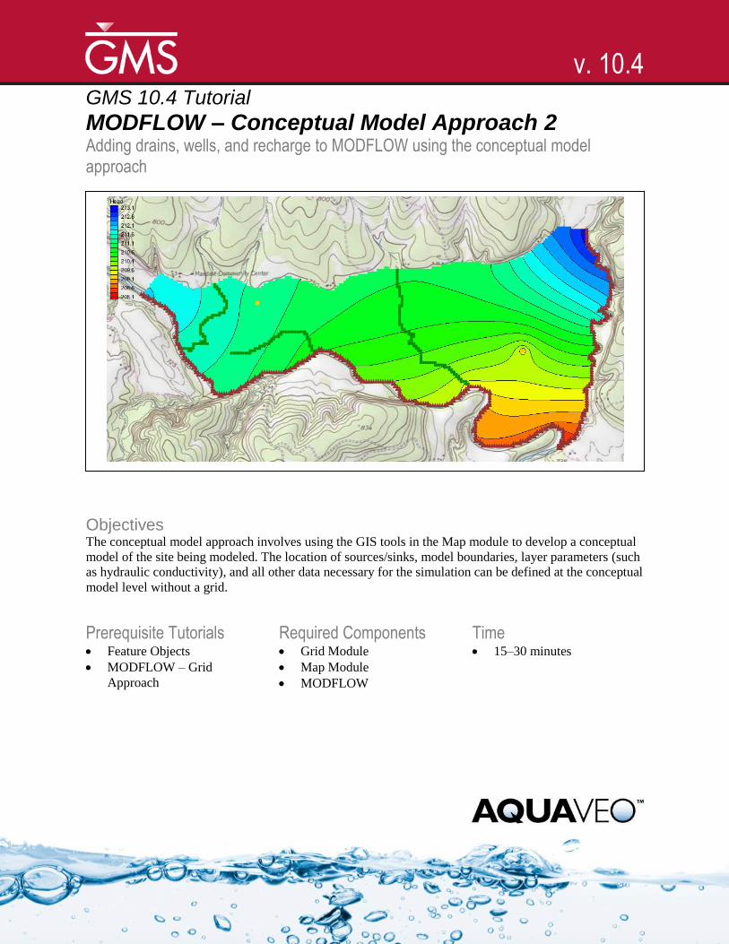
GMS 10.4 Tutorial
MODFLOW – Conceptual Model Approach 2 Adding drains, wells, and recharge to MODFLOW using the conceptual model
approach
Objectives The conceptual model approach involves using the GIS tools in the Map module to develop a conceptual
model of the site being modeled. The location of sources/sinks, model boundaries, layer parameters (such
as hydraulic conductivity), and all other data necessary for the simulation can be defined at the conceptual
model level without a grid.
Prerequisite Tutorials Feature Objects
MODFLOW – Grid
Approach
Required Components Grid Module
Map Module
MODFLOW
Time 15–30 minutes
v. 10.4

GMS Tutorials MODFLOW – Conceptual Model Approach 2
Page 2 of 13 © Aquaveo 2018
1 Introduction ......................................................................................................................... 2 1.1 Getting Started ............................................................................................................. 3
2 Importing the Project ......................................................................................................... 3 3 Saving the Project ............................................................................................................... 4 4 Delineating the Recharge Zones ......................................................................................... 4
4.1 Copying the Boundary ................................................................................................. 4 4.2 Assigning the Recharge Values .................................................................................... 5 4.3 Converting the Conceptual Model ............................................................................... 5 4.4 Checking the Simulation .............................................................................................. 5 4.5 Saving and Running MODFLOW ................................................................................ 5
5 Creating the Wells ............................................................................................................... 6 5.1 Creating the Wells Coverage ........................................................................................ 6 5.2 Creating the Well Points .............................................................................................. 6 5.3 Converting the Conceptual Model ............................................................................... 7 5.4 Checking the Simulation .............................................................................................. 7 5.5 Saving and Running MODFLOW ................................................................................ 8
6 Defining the Drain Arcs ...................................................................................................... 8 6.1 Importing the Drain Arcs ............................................................................................. 8 6.2 Assigning the Drains .................................................................................................... 9 6.3 Converting the Conceptual Model ............................................................................. 10 6.4 Checking the Simulation ............................................................................................ 11 6.5 Saving and Running MODFLOW .............................................................................. 11
7 Viewing the Solutions ........................................................................................................ 12 7.1 Viewing the Water Table in Side View ...................................................................... 12 7.2 Viewing the Flow Budget .......................................................................................... 12
8 Conclusion.......................................................................................................................... 13
1 Introduction
This tutorial builds on the “MODFLOW – Conceptual Model Approach 1” tutorial. In
that tutorial, a one-layer model using the conceptual model approach was built. The only
features assigned were the rivers, creating a simple model.
This tutorial will start with that simple model then add drains, wells, and recharge.
MODFLOW will executed after each feature is added to monitor the progressive change
in the model.
The problem this tutorial will be solving is illustrated in Figure 1. The site is located in
eastern Texas in the United States of America.
This project will be modeling the groundwater flow in the valley sediments bounded by
the hills to the north and the two converging rivers to the south. The boundary to the
north will be a no-flow boundary and the remaining boundary will be a specified head
boundary corresponding to the average stage of the rivers.
It is necessary to assume that the influx to the system is primarily through recharge due to
rainfall. There are some creek beds in the area which are sometimes dry but occasionally
fill up due to influx from the groundwater. These creek beds will be represented using
drains. Two production wells in the area will also be included in the model.
This tutorial will discuss and demonstrate:
Creating and defining drain arcs.
Creating and defining wells.

GMS Tutorials MODFLOW – Conceptual Model Approach 2
Page 3 of 13 © Aquaveo 2018
Add recharge values.
Converting the conceptual model to MODFLOW.
Checking the simulation and running MODFLOW.
Viewing the results.
River
Well #1
Well #2
River Creek beds
Limestone Outcropping
North
Figure 1 Plan view of site to be modeled
1.1 Getting Started
Do the following to get started:
1. If necessary, launch GMS.
2. If GMS is already running, select File | New to ensure that the program settings
are restored to their default state.
2 Importing the Project
The first step is to import the East Texas project. This will read in the MODFLOW
model, the solution, and all other files associated with the model.
To import the project, do as follows:
1. Click Open to bring up the Open dialog.
2. Select “Project Files (*.gpr)” from the Files of type drop-down.
3. Browse to the modfmap2 directory and select “start.gpr”.
4. Click Open to import the project and close the Open dialog.
5. Select “ Rivers” to make it active.

GMS Tutorials MODFLOW – Conceptual Model Approach 2
Page 4 of 13 © Aquaveo 2018
The Main Graphics Window will appear as in Figure 2.
Figure 2 The imported project
3 Saving the Project
Before making any changes, save the project under a new name.
1. Select File | Save As… to bring up the Save As dialog.
2. Select “Project Files (*.gpr)” from the Save as type drop-down.
3. Enter “easttex2.gpr” for the File name.
4. Click Save to save the project under the new name and close the Save As dialog.
It is recommended to Save periodically when working on projects, whether they are
tutorials or real projects.
4 Delineating the Recharge Zones
Start with constructing a coverage that defines the recharge zones. Assume that the
recharge over the area being modeled is uniform.
4.1 Copying the Boundary
To create the recharge coverage by copying the boundary coverage:
1. Right-click on the “ Boundary” coverage and select Duplicate to create a new
“ Copy of Boundary” coverage.
2. Right-click on “ Copy of Boundary” and select Properties… to bring up the
Properties dialog.
3. Enter “Recharge” as the Coverage name and click OK to close the Properties
dialog.

GMS Tutorials MODFLOW – Conceptual Model Approach 2
Page 5 of 13 © Aquaveo 2018
4. Right-click on “ Recharge” and select Coverage Setup… to bring up the
Coverage Setup dialog.
Notice that the Coverage name can be modified in this dialog as well.
5. In the Areal Properties column, turn on Recharge rate.
6. Click OK to close the Coverage Setup dialog and finish defining the recharge
coverage arcs.
7. Click Build Polygons to build the polygon on the “Recharge” coverage.
4.2 Assigning the Recharge Values
Now that the recharge zones are defined, it is possible assign the recharge values. This is
done by assigning values to the polygon.
1. Using the Select Polygons tool, double-click on the polygon to bring up the
Attribute Table dialog.
2. Enter “0.0003” as the Recharge rate.
This value was obtained by multiplying 30 inches of rainfall a year (0.75 m) by 5% and
dividing by 365.
3. Click OK to close the Attribute Table dialog.
4.3 Converting the Conceptual Model
It is now possible to convert the conceptual model from the feature object-based
definition to a grid-based MODFLOW numerical model.
1. Right-click on the “ East Texas” conceptual model and select Map To |
MODFLOW / MODPATH to bring up the Map → Model dialog.
2. Select All applicable coverages and click OK to close the Map → Model dialog.
3. Turn on “ grid” in the Project Explorer.
The recharge value has now been assigned to the cells in the 3D grid.
4.4 Checking the Simulation
At this point, the MODFLOW data is completely defined and now ready to run the
simulation. It is advisable to run the Model Checker to see if GMS can identify any
mistakes that may have been made.
1. Select MODFLOW | Check Simulation… to bring up the Model Checker dialog.
2. Click Run Check. There should be no errors.
3. Click Done to exit the Model Checker dialog.
4.5 Saving and Running MODFLOW
Save the project before running MODFLOW.
1. Save the project.

GMS Tutorials MODFLOW – Conceptual Model Approach 2
Page 6 of 13 © Aquaveo 2018
Saving the project not only saves the MODFLOW files but it saves all data associated
with the project including the feature objects and scatter points.
2. Select MODFLOW | Run MODFLOW to bring up the MODFLOW model
wrapper dialog. The model run should complete quickly.
3. When MODFLOW is finished, turn on Read solution on exit and Turn on
contours (if not on already).
4. Click Close to close the MODFLOW model wrapper dialog.
Contours should appear (Figure 3). These are contours of the computed recharge solution.
Figure 3 The contours are visible after the MODFLOW model run
5 Creating the Wells
The next step is to define the two wells. Wells are defined as point type objects.
5.1 Creating the Wells Coverage
While the wells could be added to an existing coverage, the wells will be created on a
separate coverage.
1. Right-click on the “ East Texas” conceptual model and select New
Coverage… to bring up the Coverage Setup dialog.
2. Enter “Wells” for the Coverage name.
3. In the Sources/Sinks/BCs column, turn on Wells.
4. Click OK to close the Coverage Setup dialog.
5.2 Creating the Well Points
To create the two points representing the wells and assign flow value to each of them, do
the following:

GMS Tutorials MODFLOW – Conceptual Model Approach 2
Page 7 of 13 © Aquaveo 2018
1. Right-click on the “ Wells” coverage and select the Attribute Table command
to up the Attribute Table dialog.
2. Turn on Show coordinates.
3. Under Name, enter “Well 1” then press Tab.
4. Enter the coordinates “613250” for X, “3428630” for Y, and “213” for Z pressing
the Tab key after each.
5. Select “well” from the drop-down in the Type column.
6. Enter “-50.0” in the Flow rate column.
7. On the next row down, repeat steps 3–6, entering “Well 2” for the Name,
“615494” for X, “3428232” for Y, “213.0” for Z, and “-300.0” for the Flow Rate.
8. Click OK to close the Attribute Table dialog.
The location of the wells should be as seen in Figure 4.
Figure 4 Location of the wells
5.3 Converting the Conceptual Model
Now add the wells to the MODFLOW numerical model.
1. Right-click on the “ East Texas” conceptual model and select Map To |
MODFLOW / MODPATH to bring up the Map → Model dialog.
2. Select All applicable coverages and click OK to close the Map → Model dialog.
The wells have now been added to the grid.
5.4 Checking the Simulation
Check the simulation before running MODFLOW.
1. Select MODFLOW | Check Simulation… to bring up the Model Checker dialog.
2. Click Run Check. There should be no errors.
3. Click Done to exit the Model Checker dialog.
Well #1
Well #2
GMS Tutorials MODFLOW – Conceptual Model Approach 2
Page 8 of 13 © Aquaveo 2018
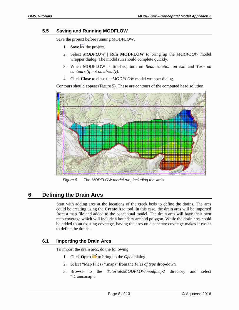
5.5 Saving and Running MODFLOW
Save the project before running MODFLOW.
1. Save the project.
2. Select MODFLOW | Run MODFLOW to bring up the MODFLOW model
wrapper dialog. The model run should complete quickly.
3. When MODFLOW is finished, turn on Read solution on exit and Turn on
contours (if not on already).
4. Click Close to close the MODFLOW model wrapper dialog.
Contours should appear (Figure 5). These are contours of the computed head solution.
Figure 5 The MODFLOW model run, including the wells
6 Defining the Drain Arcs
Start with adding arcs at the locations of the creek beds to define the drains. The arcs
could be creating using the Create Arc tool. In this case, the drain arcs will be imported
from a map file and added to the conceptual model. The drain arcs will have their own
map coverage which will include a boundary arc and polygon. While the drain arcs could
be added to an existing coverage, having the arcs on a separate coverage makes it easier
to define the drains.
6.1 Importing the Drain Arcs
To import the drain arcs, do the following:
1. Click Open to bring up the Open dialog.
2. Select “Map Files (*.map)” from the Files of type drop-down.
3. Browse to the Tutorials\MODFLOW\modfmap2 directory and select
“Drains.map”.

GMS Tutorials MODFLOW – Conceptual Model Approach 2
Page 9 of 13 © Aquaveo 2018
4. Click Open to import the project file and close the Open dialog.
GMS imports the drain arcs on their own coverage in a separate conceptual model. The
arcs will appear in the Graphics Window as shown in Figure 6.
Figure 6 Drain arcs
The drain arcs need to be added to the “ East Texas” conceptual model.
5. Select the “ Drains” coverage under the “ Drains Arcs” conceptual model.
6. Drag the “ Drains” coverage to be under the “ East Texas” conceptual
model.
7. Click Yes on the warning dialog.
8. Right-click on the “ Drains Arcs” conceptual model and select Delete.
6.2 Assigning the Drains
Next to define the arcs as drains and assign the conductance and elevation to the arcs.
1. Select the “ Drains” coverage to make it active.
2. Using the Select Arcs tool and while holding down the Shift key, select all
three drain arcs.
3. Right-click on one of the selected arcs and select Attribute Table to bring up the
Attribute Table dialog.
4. In the All row, select “drain” from the drop-down in the Type column.
5. Enter “555.0” in the Cond. (m2/d)/(m) column.
Conductance is calculated using the following formula:
L
kAC
Where k is the hydraulic conductivity, A is the gross cross-sectional area, and L is the
flow length. In this tutorial, assume that the hydraulic conductivity is 12 m/day, the drain

GMS Tutorials MODFLOW – Conceptual Model Approach 2
Page 10 of 13 © Aquaveo 2018
width is 9.25 m, and the flow length is 0.2 m. This will give a conductance of 555
(m2/day)/(m).
This represents a conductance per unit length value. GMS automatically computes the
appropriate cell conductance value when the drains are assigned to the grid cells.
6. Click OK to close the Attribute Table dialog.
The color of the drain arcs should change to show they are now recognized as drains by
GMS.
The elevations of the drains are specified at the nodes of the arcs. The elevation is
assumed to vary linearly along the arcs between the specified values.
7. Using the Select Points/Nodes tool, double-click on Node 1 as shown in
Figure 7 to bring up the Attribute Table dialog.
8. On the drain row, enter “221” in the Bot. elev. column..
9. Click OK to close the Attribute Table dialog.
10. Repeat steps 7–9 to assign the drain elevations from the list below to the rest of
the nodes shown in Figure 7.
Node 1: 221.0
Node 2: 212.0
Node 3: 220.0
Node 4: 211.0
Node 5: 221.0
Node 6: 210.0
Figure 7 Locations of the drain nodes
6.3 Converting the Conceptual Model
Now to add the arcs to the MODFLOW numerical model.
1. Right-click on the “ East Texas” conceptual model and select Map To |
MODFLOW / MODPATH to bring up the Map → Model dialog.
2. Select All applicable coverages and click OK to close the Map → Model dialog.
The Graphics Window should appear as in Figure 8.
Node 1
Node 2
Node 3
Node 4
Node 5
Node 6

GMS Tutorials MODFLOW – Conceptual Model Approach 2
Page 11 of 13 © Aquaveo 2018
Notice that the cells underlying the drains were all identified and assigned the appropriate
sources/sinks. The heads and elevations of the cells were determined by linearly
interpolating along the general head and drain arcs. The conductances of the drain cells
were determined by computing the length of the drain arc overlapped by each cell and
multiplying that length by the conductance value assigned to the arc.
Figure 8 After the conceptual model is converted to MODFLOW
6.4 Checking the Simulation
Check the simulation before running MODFLOW.
1. Select MODFLOW | Check Simulation… to bring up the Model Checker dialog.
2. Click Run Check. There should be no errors.
3. Click Done to exit the Model Checker dialog.
6.5 Saving and Running MODFLOW
Save the project before running MODFLOW.
1. Save the project.
2. Select MODFLOW | Run MODFLOW to bring up the MODFLOW model
wrapper dialog. The model run should complete quickly.
3. When MODFLOW is finished, turn on Read solution on exit and Turn on
contours (if not on already).
4. Click Close to close the MODFLOW model wrapper dialog.
Contours should appear (Figure 9). These are contours of the computed head solution.

GMS Tutorials MODFLOW – Conceptual Model Approach 2
Page 12 of 13 © Aquaveo 2018
Figure 9 The the MODFLOW model run including drains
7 Viewing the Solutions
7.1 Viewing the Water Table in Side View
Another interesting way to view a solution is in side view.
1. Turn off “ Grid Frame” in the Project Explorer.
2. Select “ MODFLOW” in the Project Explorer to switch to the 3D Grid
module.
3. Using the Select Cell tool, select a cell somewhere near the well on the right
side of the model.
4. Switch to Side View .
5. Click Frame Image .
Notice that the computed head values are used to plot a water table profile.
6. Use the arrow buttons in the main toolbar to move back and forth through the
grid. A cone of depression should be seen at the well.
7. When finished, switch to Plan View .
7.2 Viewing the Flow Budget
The MODFLOW solution consists of both a head file and a cell-by-cell flow (CCF) file.
GMS can use the CCF file to display flow budget values. To know if any water exited
from the drains, simply click on a drain arc.
1. Select the “ Map Data” folder in the Project Explorer.
2. Using the Select Arcs tool, select the rightmost drain arc.

GMS Tutorials MODFLOW – Conceptual Model Approach 2
Page 13 of 13 © Aquaveo 2018
Notice that the total flow through the arc is displayed in the strip at the bottom left of the
window. Next, view the flow to the river.
3. Click on one of the specified head arcs at the bottom and view the flow.
4. Hold down the Shift key and select all of the specified head arcs.
Notice that the total flow is shown for all selected arcs. Flow for a set of selected cells
can be displayed as follows:
5. Select the “ 3D Grid Data” folder in the Project Explorer.
6. Select a group of cells by dragging a box around the cells.
7. Select MODFLOW | Flow Budget... to bring up the Flow Budget dialog.
The Flow Budget dialog shows a comprehensive flow budget for the selected cells.
8. Click OK to exit the Flow Budget dialog.
9. Click anywhere outside the model to unselect the cells.
8 Conclusion
This concludes the “MODFLOW – Conceptual Model Approach 2” tutorial. Here are the
Key concepts from this tutorial:
Feature arcs can be used to define drains in the conceptual model.
Feature points can be used to define wells in the conceptual model.
Feature polygons can be used to define recharge areas in the conceptual model.
It is possible to customize the set of properties associated with points, arcs and
polygons by using the Coverage Setup dialog.
It is necessary to use the Map → MODFLOW / MODPATH command every
time that conceptual model data is transferred to the grid.