gnss ionospheric scintillations classification by machine
TRANSCRIPT

Polytechnic University of TurinDepartment of Electronics and Telecommunications
ICT for Smart Societies Master of Science Degree
GNSS Ionospheric ScintillationsClassification by Machine Learning
Presented by: BADIAA MAKHLOUF Supervised by: PR. FABIO DOVIS
MARCH 2019


DEDICATION AND ACKNOWLEDGEMENTS
Ffirstly, I want to express my gratitude to Pr. Fobio Dovis for the time he has devoted me,during this experience, to ensure all the parts of my thesis. Furthermore, I would like tothank him for his assistance, his availability and his guidance that allowed me to move
forward, to well-written my report and to reach my target goals.
Also, I would like to acknowledge my parents and my brother for their unfailing support andcontinuous encouragement during my master studies. This accomplishment would not have beenpossible without them.
Thank you all!
i


ABSTRACT
GNSS Ionospheric Scintillations Classification by Machine Learning
The ionospheric scintillations influence transionospheric radio waves propagation in theatmosphere, which leads to positioning errors and GNSS performance degradation. Pre-viously, the scintillations detection was based on traditional techniques analyzing some
scintillation indices, S4 (amplitude scintillation indicator) and φ60 (phase scintillation indicator),from the received signals and comparing them to thresholds. Unfortunately, those approachessuffer from many limitations. This thesis aims to enhance the ISM receiver operation throughdeveloping an automatic approach to detect amplitude or phase fluctuations originated fromscintillation events and identifying them by means of Machine Learning (ML) classificationalgorithms. In effect, ionospheric irregularities are sometimes indistinguishable from multipathor interference disturbances and the ML was an effective solution to differentiate between themand to avoid their positioning error. Previous papers have presented the binary classificationof GPS L1C/A data by the Support Vector Machine (SVM), which was used to indicate whetherscintillation exists or no. In this report, five classes were used that are : non-scintillation, low,moderate, strong and multipath. The three algorithms that were applied over a set of collectedGPS L1C/A, low and high rate, data by means of ISMR in the Antarctica continent are the C4.5Decision Tree, the Bagged Trees and the Neural Network implemented by sklearn, MATLABand TensorFlow, respectively. The ISMR standard output is either a post-processing file, whichis composed by 62 parameters where the S4, φ60 and the time are among them, or it is a rowdata file, which contains 12 parameters. In the first step, only 12 features were selected from the62 parameters. Next to the 12 picked features, a class label from the five previously mentionedclasses was manually assigned to each observation in the input data. In the second step, eachobservation contains next to the class label, the spectral contents that were obtained via applyingthe Short Time Fourier Transform (STFT) over 3 minutes blocks of S4 or φ60 measurements.This thesis consists on predicting the class from the remained attributes and on confirminghow detection could be done over a reduced number of features so no need to integrate all theparameters. Moreover, this work demonstrates that attributes with larger dimensions like thePower Spectral Density (PSD) are more reliable to distinguish scintillation levels: low, moderateand strong that influence phase or amplitude measurements. To evaluate results, the confusionmatrix, the testing and the training accuracies have been utilized.Keywords: GNSS, GPS, ML, multi-class classification, multipath, neural network (TensorFlow),C4.5 (sklearn), Bagged Trees (MATLAB), PSD, STFT, ionospheric scintillations indexes (S4 andφ60).
ii


RIASSUNTO
Classificazione delle Scintillazioni Ionosferiche del GNSS tramite il MachineLearning
Le scintillazioni ionosferiche influenzano la propagazione delle onde radio transionosferichenell’atmosfera, il che porta a errori di posizionamento e il degrado delle prestazioni delGNSS. In precedenza, il rilevamento delle scintillazioni si basava su tecniche tradizionali
come l’analisi degli indicatori di scintillazione S4 (indicatore di scintillazione di ampiezza) e φ60(indicatore di scintillazione di fase), dai segnali ricevuti e confrontandoli con le soglie. Sfortu-natamente, questi approcci hanno molte limitazioni. Questa tesi mira a migliorare l’operativitàdel ricevitore ISM rilevando automaticamente fluttuazioni di ampiezza o di fase originate daeventi di scintillazione e identificandole mediante algoritmi ML (Machine Learning) di classifi-cazione. In effetti, le irregolarità ionosferiche sono talvolta indistinguibili da disturbi multipatho interferenze e la ML è una soluzione efficace per distinguerle e stimare il loro errore di po-sizionamento. Gli articoli precedenti avevano presentato la classificazione binaria dei dati GPSL1C/A eseguita con Support Vector Machine (SVM) per indicare se la scintillazione esiste o no. Inquesto rapporto, sono state utilizzate cinque classi: non scintillazione, bassa, moderata, forte emultipath. I seguenti tre algoritmi sono stati applicati su un insieme di dati GPS L1C/A raccoltia bassa e alta velocità mediante ISMR nel continente Antartico, gli Alberi decisionali C4.5, gliBagged Trees e la rete neurale implementati da sklearn, MATLAB e TensorFlow, rispettivamente.L’output standard ISMR può essere un file di post-elaborazione, composto da 62 parametri in cuiS4, φ60 e il tempo o può essere un file di dati di riga, che contiene 12 parametri. Nella prima fasesono state selezionate solo 12 caratteristiche tra i 62 parametri. Accanto alle 12 Caratteristicheselezionate, una delle cinque classi citate in precedenza è stata assegnata manualmente ad ogniosservazione nei dati di input. Nella seconda fase, ogni osservazione contiene accanto alla classe,i contenuti spettrali che sono stati ottenuti attraverso l’applicazione della Trasformata di Fouriera Tempo Breve (STFT) su blocchi di 3 minuti di misurazioni di S4 o φ60. Questa tesi consistenel dedurre la classe tramite gli attributi rimasti e nel confermare come il rilevamento potrebbeessere eseguito su un numero ridotto di funzionalità e senza la necessità di integrare tutti iparametri. Inoltre, dimostra che gli attributi con dimensioni maggiori come Densità spettrale dipotenza (PSD) sono più affidabili per distinguere i livelli di scintillazione: bassa, moderata e forteche influenzano le misurazioni di fase o ampiezza. Per valutare i risultati sono stati utilizzati lamatrice di confusione e la precisione del modello.Parole chiave: GNSS, GPS, ML, classificazione multi-class, multipath, rete neurale (Tensor-Flow), C4.5 (sklearn), Bagged Trees (MATLAB), PSD, STFT, indici di scintillazioni (S4 and φ60).
iii


RÉSUMÉ
Classification des scintillations ionosphériques du GNSS par apprentissageautomatique
Les scintillations ionosphériques influencent la propagation des ondes radio transionosphériquesce qui provoque des erreurs de positionnement et une dégradation des performances duGNSS. Auparavant, des techniques traditionnelles ont été utilisées pour détecter les scintil-
lations telles que l’analyse du S4 (l’indicateur de scintillation d’amplitude) et du φ60 (l’indicateurde scintillation de phase) et les comparer aux seuils. Malheureusement ces approches sont lim-itées par example elles demandent beaucoup du temps et sont pas automatiques. Ce travail vise àaméliorer le fonctionnement d’un récepteur ISM en lui permettant de détecter automatiquementles fluctuations d’amplitude ou de phase, suite à un événements de scintillations, à l’aide des al-gorithmes implémentés par l’apprentissage automatique appellé Machine Learning (ML). Parfois,les irrégularités ionosphériques sont indiscernables des trajets multiples ou des interférences.Cependant, le ML permet d’identifier la différence entre eux et ensuite permet d’estimer leurerreurs de positionnement afin de les corriger. Avant, la classification des données GPS L1C/A aété présentée mais en utilisant seulement deux classes avec la machine à vecteurs de support(SVM). Dans ce rapport, des données GPS L1C/A ont été classifiées en cinq catégories dont: nonscintillation, faible, modérée, forte et trajets multiples. Les trois algorithmes suivants ont étéappliqués, l’arbres de décision de C4.5 implémentés par sklearn, le Bagged Trees implémentéspar MATLAB et le Neural Network implémenté par TensorFlow. Le deux types de fichiers desortie ISMR ont été utilisés qui sont les fichiers de post-traitement et les fichiers de donnéesbrutes. Les fichiers de post-traitement sont composés de 62 paramètres dont les valeurs S4,φ60 et le temps. Lors de la première étape, seules 12 attribues ont été sélectionnés parmi les62 paramètres. Outre les 12 caractéristiques sélectionnées, une étiquette de classe parmi lescinq classes mentionnées peu avant a été attribuée manuellement à chaque observation. Dansla deuxiéme étape, la prédiction d’étiquette a été effectuée par les composantes du domainefréquentiel obtenus suite à l’application de la Transformée de Fourier à Court Terme (TFCT) surS4 ou φ60. Ce mémoire consiste à prédire la classe à partir des attributs restants. Aussi, il essaiede démontrer que l’analyse peut être basée sur un nombre réduit des attributs et à demontrer lafiabilité de la densité spectrale de puissance (DSP) pour distinguer les niveaux de scintillation:faible, modérée et forte qui influencent la phase ou l’amplitude. Pour évaluer tous les résultats,la matrice de confusion, les précisions d’entraînement et de tests ont été illustrées.Keywords: GNSS, GPS, ML, multi-class classification, trajets multiples, réseau de neurones(TensorFlow), C4.5 (sklearn), Bagged Trees (MATLAB), densité spectrale de puissance, Transfor-mée de Fourier à court terme, indices de scintillations ionosphériques (S4 and φ60).
iv


LIST OF ACRONYMS
A/D Analog to Digital
ANN Artificial Neural Network
BT Bagged Trees
C/A Coarse/Acquisition
CR Cognitive Radio
demoGRAPE demonstrator GNSS Research and Application for Polar Environment
DVB-T Digital Video Broadcasting- Terrestrial
EGNOS European Geostationary Navigation Oerlay Service
ERM Empirical Risk Minimization
GNSS Global Navigation Satellite System
GPS Global Positioning System
HF High Frequency
IF Intermediate Frequency
ISMR Ionospheric Scintillation Monitoring Receiver
KNN K Nearest Neighbor
LoS Line of Sight
LS Least Squares
ML Machine Learning
MSE Minimum Square Error
NavSAS Navigation Signal Analysis and Simulation
NN Neural Network
NLoS Non Line of Sight
PCA Principal Component Analysis
PDF Probability Density Function
v

PRN Pseudo Random Noise
PSD Power Spectral Density
RF Random Forest
RFI Radio Frequency Interference
SDR Software Defined Radio
SNR Signal to Noise Ratio
SRM Structural Risk Minimization
STFT Short Time Fourrier Transform
SVM Support Vector Machine
SVID Satellite Vehicle IDentification
TEC Total Electron Content
UHF Ultra High Frequency
UWB Ultra Wide Band
vi

TABLE OF CONTENTS
Page
List of Tables ix
List of Figures x
General Introduction 1
1 State of the art 2Introduction . . . . . . . . . . . . . . . . . . . . . . . . . . . . . . . . . . . . . . . . . . . . . . 2
1.1 Global Navigation Satellite System: GNSS . . . . . . . . . . . . . . . . . . . . . . . . 2
1.1.1 GNSS operating principles . . . . . . . . . . . . . . . . . . . . . . . . . . . . . 3
1.1.2 GNSS signals impairments . . . . . . . . . . . . . . . . . . . . . . . . . . . . . 5
1.2 Machine learning and Ionospheric Scintillations detection . . . . . . . . . . . . . . 9
1.2.1 Machine learning . . . . . . . . . . . . . . . . . . . . . . . . . . . . . . . . . . . 9
1.2.2 Current methods for Ionospheric Scintillations detection . . . . . . . . . . . 9
Conclusion . . . . . . . . . . . . . . . . . . . . . . . . . . . . . . . . . . . . . . . . . . . . . . . 15
2 Preliminary analysis 16Introduction . . . . . . . . . . . . . . . . . . . . . . . . . . . . . . . . . . . . . . . . . . . . . . 16
2.1 Dataset description . . . . . . . . . . . . . . . . . . . . . . . . . . . . . . . . . . . . . . 16
2.1.1 Low rate features . . . . . . . . . . . . . . . . . . . . . . . . . . . . . . . . . . 17
2.1.2 High rate features . . . . . . . . . . . . . . . . . . . . . . . . . . . . . . . . . . 19
2.2 Validation techniques, dimensionality reduction and confusion matrix . . . . . . . 21
2.2.1 Validation techniques . . . . . . . . . . . . . . . . . . . . . . . . . . . . . . . . 21
2.2.2 Dimensionality reduction by PCA . . . . . . . . . . . . . . . . . . . . . . . . . 22
2.2.3 Confusion matrix . . . . . . . . . . . . . . . . . . . . . . . . . . . . . . . . . . . 22
2.3 Multiclass classification algorithms: . . . . . . . . . . . . . . . . . . . . . . . . . . . . 24
2.3.1 MATLAB classificationLearner app . . . . . . . . . . . . . . . . . . . . . . . 24
2.3.2 Bagged Trees :BT . . . . . . . . . . . . . . . . . . . . . . . . . . . . . . . . . . . 28
2.3.3 C4.5 Decision Tree . . . . . . . . . . . . . . . . . . . . . . . . . . . . . . . . . . 29
2.3.4 Neural Network . . . . . . . . . . . . . . . . . . . . . . . . . . . . . . . . . . . 39
vii

TABLE OF CONTENTS
Conclusion . . . . . . . . . . . . . . . . . . . . . . . . . . . . . . . . . . . . . . . . . . . . . . . 46
3 Results and discussion 47Introduction . . . . . . . . . . . . . . . . . . . . . . . . . . . . . . . . . . . . . . . . . . . . . . 47
3.1 Ionospheric scintillation automatic detection based on absolute values of scintilla-
tion indicators S4 and φ60 . . . . . . . . . . . . . . . . . . . . . . . . . . . . . . . . . . 47
3.1.1 Bagged Trees . . . . . . . . . . . . . . . . . . . . . . . . . . . . . . . . . . . . . 49
3.1.2 C4.5 Decision Tree . . . . . . . . . . . . . . . . . . . . . . . . . . . . . . . . . . 53
3.1.3 Neural Network . . . . . . . . . . . . . . . . . . . . . . . . . . . . . . . . . . . 56
3.1.4 Conclusions in this study . . . . . . . . . . . . . . . . . . . . . . . . . . . . . . 59
3.2 Ionospheric scintillation automatic detection based on the frequency domain fea-
tures of scintillation indicators S4 and φ60 . . . . . . . . . . . . . . . . . . . . . . . 60
3.2.1 Bagged Trees . . . . . . . . . . . . . . . . . . . . . . . . . . . . . . . . . . . . . 61
3.2.2 C4.5 Decision Tree . . . . . . . . . . . . . . . . . . . . . . . . . . . . . . . . . . 64
3.2.3 Neural Network . . . . . . . . . . . . . . . . . . . . . . . . . . . . . . . . . . . 69
3.2.4 Conclusions in this study . . . . . . . . . . . . . . . . . . . . . . . . . . . . . . 74
Conclusion . . . . . . . . . . . . . . . . . . . . . . . . . . . . . . . . . . . . . . . . . . . . . . . 75
General conclusion 76
A Appendix 78
Bibliography 81
viii
LIST OF TABLES
TABLE Page
2.1 Class consideration for amplitude and phase scintillations intensity . . . . . . . . . . 20
2.2 Training accuracies before and after PCA with 25% holdout validation technique . . . 25
2.3 Training accuracies before and after PCA with 5-fold cross validation technique . . . 26
2.4 Training accuracies for various classification algorithms with no validation, 5-fold
cross validation and 25% holdout validation . . . . . . . . . . . . . . . . . . . . . . . . . 27
2.5 Comparaison between the classification importance of the considered features in case
1 (sorted data) and case 2 (random data) . . . . . . . . . . . . . . . . . . . . . . . . . . . 33
2.6 Comparaison between the classification importance of the considered features in case
1 (sorted data) and case 2 (random data) with and without the time attribute integration 34
2.7 Comparaison between features importance in the classification process using random
data case and different training data sizes . . . . . . . . . . . . . . . . . . . . . . . . . . 35
2.8 Training accuracies adopting different initial learning coefficients and iterations
number of the Gradient Descent . . . . . . . . . . . . . . . . . . . . . . . . . . . . . . . . 42
2.9 Testing and training accuracies considering 10−4 as initial learning coefficient with
various training data sizes . . . . . . . . . . . . . . . . . . . . . . . . . . . . . . . . . . . . 44
3.1 Number of cases identifying each class, in the first input dataset, based on absolute
values of scintillations indicators, S4 and φ60 . . . . . . . . . . . . . . . . . . . . . . . . 48
3.2 Testing and training accuracies considering input data based on absolute values of
scintillation indicators, S4 and φ60, with various training dataset sizes for the three
selected methods . . . . . . . . . . . . . . . . . . . . . . . . . . . . . . . . . . . . . . . . . . 48
3.3 Samples number per each class in the second input dataset, which was based on the
frequency domain features of scintillation indicators, S4 or φ60, for both amplitude or
phase scintillation detection cases . . . . . . . . . . . . . . . . . . . . . . . . . . . . . . . 61
3.4 Testing and training accuracies considering 80% of total provided data, based on PSD
of S4, to train the generated model for the three selected methods . . . . . . . . . . . . 74
3.5 Testing and training accuracies considering 80% of total provided data, based on PSD
of φ60, to train the generated model for the three selected methods . . . . . . . . . . . 74
ix


LIST OF FIGURES
FIGURE Page
1.1 Examples of the GNSS satellite constellation . . . . . . . . . . . . . . . . . . . . . . . . 3
1.2 GNSS receiver functional scheme . . . . . . . . . . . . . . . . . . . . . . . . . . . . . . . . 4
1.3 GNSS Position estimation by means of four LoS satellites . . . . . . . . . . . . . . . . . 5
1.4 Illustration of signal disturbances due to ionospheric scintillations and of TEC mea-
surements . . . . . . . . . . . . . . . . . . . . . . . . . . . . . . . . . . . . . . . . . . . . . . 6
1.5 Reflected signals due to multipath . . . . . . . . . . . . . . . . . . . . . . . . . . . . . . . 7
1.6 Atmospheric layers . . . . . . . . . . . . . . . . . . . . . . . . . . . . . . . . . . . . . . . . 8
1.7 Traditional ionospheric detection approaches . . . . . . . . . . . . . . . . . . . . . . . . . 10
1.8 The SVM classifier [14] . . . . . . . . . . . . . . . . . . . . . . . . . . . . . . . . . . . . . . 12
1.9 The overall validation accuracy of the SVM detectors in [14] . . . . . . . . . . . . . . . 13
1.10 Flow diagram of the applied ML process composed by the learning and the classifica-
tion phases [24] . . . . . . . . . . . . . . . . . . . . . . . . . . . . . . . . . . . . . . . . . . 15
2.1 GPS station in Antarctica . . . . . . . . . . . . . . . . . . . . . . . . . . . . . . . . . . . . 17
2.2 SVID corresponding to each GNSS constellation from the PolaRxS application manual 18
2.3 Confusion matrix structure . . . . . . . . . . . . . . . . . . . . . . . . . . . . . . . . . . . 23
2.4 BT training accuracies for various reduced number of features using PCA . . . . . . . 27
2.5 Diagram flow of the BT algorithm . . . . . . . . . . . . . . . . . . . . . . . . . . . . . . . 28
2.6 BT confusion matrix implementing different validation techniques . . . . . . . . . . . 29
2.7 An example of decision tree generated by C4.5 . . . . . . . . . . . . . . . . . . . . . . . . 30
2.8 Diagram flow of the C4.5 algorithm . . . . . . . . . . . . . . . . . . . . . . . . . . . . . . 31
2.9 C4.5 features importances in the classification process when the data was sorted . . . 32
2.10 C4.5 features importances in the classification process when the data was random . . 32
2.11 C4.5 training and testing accuracies as function of decision tree depth . . . . . . . . . 36
2.12 C4.5 training and testing accuracies as function of minimum number of samples per
internal node . . . . . . . . . . . . . . . . . . . . . . . . . . . . . . . . . . . . . . . . . . . . 37
2.13 C4.5 training and testing accuracies as function of minimum number of samples per
leaf node . . . . . . . . . . . . . . . . . . . . . . . . . . . . . . . . . . . . . . . . . . . . . . . 37
2.14 C4.5 training and testing accuracies as function of features maximum number . . . . 38
x

LIST OF FIGURES
2.15 The artificial neuron structure versus the brain neuron structure . . . . . . . . . . . . 39
2.16 The ANN architecture . . . . . . . . . . . . . . . . . . . . . . . . . . . . . . . . . . . . . . 39
2.17 Diagram flow of the NN (TF) algorithm . . . . . . . . . . . . . . . . . . . . . . . . . . . . 41
2.18 NN training accuracies with devoting 50% of total data to training phase and consid-
ering various learning coefficients for the Gradient Descent algorithm . . . . . . . . . 42
2.19 NN training and testing accuracies with devoting 50% of total input data for each phase 45
2.20 NN training and testing accuracies with devoting 80% of total input data for each phase 46
3.1 The first set of employed features, in the elaborated work, based on the absolute values
of S4 and φ60 measurements . . . . . . . . . . . . . . . . . . . . . . . . . . . . . . . . . . 48
3.2 The BT confusion matrices obtained after activating the 5-fold cross validation tech-
nique considering 50% of input dataset during training phase . . . . . . . . . . . . . . 50
3.3 The BT confusion matrices obtained after activating the 5-fold cross validation tech-
nique considering 80% of input dataset during training phase . . . . . . . . . . . . . . 51
3.4 The obtained BT confusion matrices considering 50% of dataset size in the training
stage with and without the time attribute integration in the features set . . . . . . . . 52
3.5 The obtained C4.5 confusion matrices considering 50% of total data in the training stage 53
3.6 The obtained C4.5 testing confusion matrices considering different training dataset
sizes; 50% and 80% of total input data . . . . . . . . . . . . . . . . . . . . . . . . . . . . . 54
3.7 The obtained C4.5 testing confusion matrices with excluding the time feature and
with considering different training dataset sizes: 50% and 80% of total input data . . 55
3.8 The obtained training and testing NN confusion matrices in case 50% of total provided
data was used to train the model . . . . . . . . . . . . . . . . . . . . . . . . . . . . . . . . 56
3.9 The obtained training and testing confusion matrices by NN in case 80% of total
provided data was used to train the model . . . . . . . . . . . . . . . . . . . . . . . . . . 57
3.10 The obtained NN confusion matrices considering 50% of total input dataset size in the
training stage with and without the time attribute integration in the features set . . 58
3.11 The obtained BT training and testing confusion matrices considering 80% of the total
input data based on S4 PSD components to train the model . . . . . . . . . . . . . . . . 62
3.12 The obtained BT training and testing confusion matrices considering 80% of the total
input data based on φ60 PSD components to train the model . . . . . . . . . . . . . . . 63
3.13 The C4.5 training and testing accuracies as function of decision tree depth considering
80% of the total input data based on S4 PSD components . . . . . . . . . . . . . . . . . 65
3.14 The C4.5 training and testing accuracies as function of minimum number of samples
required to split an internal node considering 80% of the total input data based on S4
PSD components . . . . . . . . . . . . . . . . . . . . . . . . . . . . . . . . . . . . . . . . . . 65
3.15 The C4.5 training and testing accuracies as function of minimum number of samples
required to form a leaf node considering 80% of the total input data based on S4 PSD
components . . . . . . . . . . . . . . . . . . . . . . . . . . . . . . . . . . . . . . . . . . . . . 66
xi

LIST OF FIGURES
3.16 The obtained C4.5 training and testing confusion matrices considering 80% of the
total input data based on S4 PSD components to train the model . . . . . . . . . . . . . 66
3.17 Training and testing accuracies as function of tree depth . . . . . . . . . . . . . . . . . 68
3.18 Training and testing accuracies as function of minimum number of samples required
to split an internal node . . . . . . . . . . . . . . . . . . . . . . . . . . . . . . . . . . . . . 68
3.19 Training and testing accuracies as function of minimum number of samples required
to form a leaf node . . . . . . . . . . . . . . . . . . . . . . . . . . . . . . . . . . . . . . . . . 68
3.20 The obtained C4.5 training and testing confusion matrices considering 80% of total
input data based on φ60 PSD components to train the model and after fixing the
tuning parameters . . . . . . . . . . . . . . . . . . . . . . . . . . . . . . . . . . . . . . . . . 69
3.21 The NN classification training accuracy versus Gradient Descent iterations number
with adopting different initial learning coefficients over 80% of the provided data
based on PSD components, acquired from S4, to generate the trained model . . . . . . 70
3.22 NN training and testing accuracies with 80% of total PSD components, acquired from
S4, devoted for training phase and with initial learning rate equal to 10−6 . . . . . . . 70
3.23 The NN obtained training and testing confusion matrices considering 80% of total
input data based on S4 PSD features to train the model . . . . . . . . . . . . . . . . . . 71
3.24 The NN classification training accuracy versus Gradient Descent iterations number
with adopting different initial learning coefficients over the 80% of input data based
on PSD components, acquired from φ60, to generate the trained model . . . . . . . . . 72
3.25 NN training and testing accuracies with 80% of total input data based on PSD
components, acquired from φ60, devoted for training phase and with initial learning
rate equal to 10−5 . . . . . . . . . . . . . . . . . . . . . . . . . . . . . . . . . . . . . . . . . 73
3.26 The NN obtained training and testing confusion matrices considering 80% of total
input data, based on φ60 PSD features, to train the model . . . . . . . . . . . . . . . . . 73
xii

GENERAL INTRODUCTION
Nowadays, localization has gained a great standing for industry, research and civil domains.Therefore, a huge number of localization-based applications was seen during the lastdecades. In fact, efficient localization services are needed for both indoor and outdoor
areas. Besides, indoor localization is achieved by means of wireless technologies such as Bluetoothbeacons, wireless sensor networks and Wi-Fi hotspots while the outdoor localization is morebased on the received signals from the Global Navigation Satellite System (GNSS).
For the outdoor localization, many factors are affecting the radio wave propagation and soon the position accuracy. In addition, those factors are producing the degradation of the GNSSsystem, such as GPS, precision and performance. The ionospheric scintillations are one of themajor origins of the GNSS signal perturbations especially at equatorial and high latitudes areas.
Moreover, not only ionospheric scintillations influence the signal propagation from the satel-lite to the receiver but also interference and multipath have certain impacts. Thus, it is veryimportant to identify whether the received signal was scratched or not and in case it was, itis required to differentiate between the various types of disturbances. In many situations, thecrucial issue is that ionospheric scintillations are indistinguishable from the multipath and theinterference phenomena.
For the reason that the ionospheric scintillations have the greatest impact on GNSS sys-tem execution, the early and the accurate detection of such events is very advantageous formany applications like space weather applications, safe aeronautical operations, atmosphericremote sensing and developing robust detection algorithms for GNSS receivers. Currently, sev-eral traditional approaches are existing and they have been used during the previous years butunfortunately they are presenting many insufficiencies.
More precisely, the elaborated detection process consists on assigning each of the received GPSsignals to one category among the various existing classes, in the input data, where each classidentifies the signal status. The ML was a good, an automatic and a fast solution to differentiatebetween scintillations levels and multipath.
This report comports three chapters with a general introduction and a general conclusion. Thefirst chapter was dedicated to the state of the art presentation, the second chapter was devotedfor discussing the preliminary analysis while the results and interpretations were detailed in thethird chapter.
1


CH
AP
TE
R
1STATE OF THE ART
Introduction
One of the main problems in the GNSS positioning systems are the signals measurements
variations, which must be detected and corrected. A ML approach could be an effective
solution to ease the detection and the identification process. First of all, it would be
a good idea to highlight, in the first part of this chapter, the main sources of GNSS signals
disturbances while the second part was used to present a review about the already applied ML
approaches in this field.
1.1 Global Navigation Satellite System: GNSS
The GNSS is a satellite constellation used for geospatial positioning through regularly acquiring
time signals from satellites and analyzing them by commercial or professional receivers on the
earth. The first GNSS system was invented by the US department of defense and it is called
Global Positioning System (GPS). At the begning, it was only dedicated for military services but
now it is open to the civil and the industrial applications.
After the technological revolution and with the implementation of this technology in the
smart items, such as Smartphones and Tablets, it became more accessible and more demanded.
That’s why many new GNSS systems, like the two European systems: the European Global Satel-
lite Navigation System (Galileo) and the European Geostationary Navigation Overlay Service
(EGNOS), the Russian system: the Global Orbiting Navigation Satellite System (GLONASS)
and the Chinese one BeiDou, have appeared. The most important point that all of them are
iteroperable with GPS.
2
1.1. GLOBAL NAVIGATION SATELLITE SYSTEM: GNSS
(a) (b)
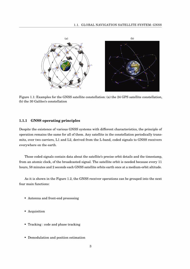
Figure 1.1: Examples for the GNSS satellite constellation: (a) the 24 GPS satellite constellation,(b) the 30 Galileo’s constellation
1.1.1 GNSS operating principles
Despite the existence of various GNSS systems with different characteristics, the principle of
operation remains the same for all of them. Any satellite in the constellation periodically trans-
mits, over two carriers, L1 and L2, derived from the L-band, coded signals to GNSS receivers
everywhere on the earth.
Those coded signals contain data about the satellite’s precise orbit details and the timestamp,
from an atomic clock, of the broadcasted signal. The satellite orbit is needed because every 11
hours, 58 minutes and 2 seconds each GNSS satellite orbits earth once at a medium-orbit altitude.
As it is shown in the Figure 1.2, the GNSS receiver operations can be grouped into the next
four main functions:
• Antenna and front-end processing
• Acquisition
• Tracking : code and phase tracking
• Demodulation and position estimation
3

CHAPTER 1. STATE OF THE ART
Figure 1.2: GNSS receiver functional scheme
The antenna acquires the signal and forwards it to the front-end unit, to move its High Frequency
(HF) to an Intermediate Frequency (IF), then to perform the analog to digital (A/D) conversion
through sampling and quantizing it. At the end, the signal is filtered from the noise.
The acquisition stage consists on performing the initial estimate of the delay between the
incoming code, from the satellite, and the locally generated replica by the receiver. The delay
calculation is based on the broadcasting timestamp carried by the received signal. In addition,
the acquisition stage allows the estimation of the Doppler shift on the carrier.
The tracking stage aims to keep synchronization between the previous two codes by dynam-
ically recover the delay between them. In addition, it aims to refine the Doppler shift and the
phase to increase the position accuracy.
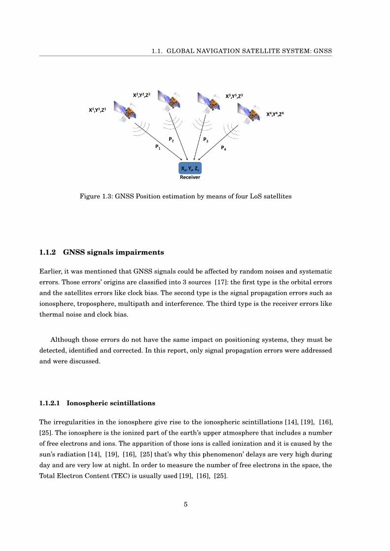
As it is displayed in the Figure 1.3, the position estimation is based on the transmitted codes
from at least four satellites in Line of sight (LoS). Those codes allow the identification of the
satellites locations and allow the computation of the delay difference as it was mentioned in the
acquisition stage. Ultimately, this delay is translated to the distance or to the range between
the satellite and the receiver. Once the receiver gets its accurate position with respect to the
four satellites in view, it transforms this position to latitude, longitude and height within the
Earth-based coordinates system.
4
1.1. GLOBAL NAVIGATION SATELLITE SYSTEM: GNSS
Figure 1.3: GNSS Position estimation by means of four LoS satellites
1.1.2 GNSS signals impairments
Earlier, it was mentioned that GNSS signals could be affected by random noises and systematic
errors. Those errors’ origins are classified into 3 sources [17]: the first type is the orbital errors
and the satellites errors like clock bias. The second type is the signal propagation errors such as
ionosphere, troposphere, multipath and interference. The third type is the receiver errors like
thermal noise and clock bias.
Although those errors do not have the same impact on positioning systems, they must be
detected, identified and corrected. In this report, only signal propagation errors were addressed
and were discussed.
1.1.2.1 Ionospheric scintillations
The irregularities in the ionosphere give rise to the ionospheric scintillations [14], [19], [16],
[25]. The ionosphere is the ionized part of the earth’s upper atmosphere that includes a number
of free electrons and ions. The apparition of those ions is called ionization and it is caused by the
sun’s radiation [14], [19], [16], [25] that’s why this phenomenon’ delays are very high during
day and are very low at night. In order to measure the number of free electrons in the space, the
Total Electron Content (TEC) is usually used [19], [16], [25].
5

CHAPTER 1. STATE OF THE ART
(a) (b)
Figure 1.4: Illustration of: (a) signal disturbances due to Ionospheric Scintillations, (b) freeelectrons measurements by TEC.
The TEC is defined as the number of electrons in a tube of 1m2 cross section from receiver
to satellite [14], [19], [16]. The GNSS signals propagation delay depends on the TEC along
the path, as it is shown in the Figure 1.4 and the latter depends on the ionospheric plasma
irregularities [19], [16], [25]. If the TEC value is very high it causes diffraction or refraction of
the original signal [14], [19], [16], [25], which is equivalent to rapid phase and/or amplitude
fluctuations. The phase fluctuations consist on increasing carrier phase cycle slips while the
amplitude variations consist on increasing a carrier tracking loop errors and an amplitude fading
tracking loop errors [14] [24]. Both of those variations, induce positioning errors in the order of
ten meters [14] [24].
The scintillations levels and occurrence depend on many factors such as the geographic
location, the epoch of the year, the signal frequency, the local time and the solar cycle [5], [19].
Not always, the ionospheric scintillations are the origins of the GNSS positioning errors but
sometimes the errors are caused by multipath, interference or tropospheric effects [5], [19], [16],
[25].
1.1.2.2 Multipath
Multipath is one of the errors sources in GNSS positioning system and it has a large negative
effect especially on signals broadcasted by Galileo and GPS constellations [17]. It limits the
performance of the system due to the deviation of the direct rays [3], called the LoS signals, as it
is presented in the Figure 1.5.
In actual fact, the deviation includes the LoS signal reflection through following various paths.
Therefore, the received signal is no more the direct one but it becomes a combination between
6

1.1. GLOBAL NAVIGATION SATELLITE SYSTEM: GNSS
direct signal and its reflected versions [3]. However, the position information is only carried by
the LoS signal while the other components are noises and they must be discarded.
Figure 1.5: Reflected signals due to multipath
Furthermore, the interference produced by multipath could be classified into two categories:
the first type is a Non Line of Sight (NLoS) interference that corresponds to the reception of a
unique delayed signal while the second type is a light of sight interference, which corresponds to
the combination of the direct signal with its delayed versions [3].
Several research projects have been developped for finding an appropriate and an efficient
technique to mitigate multipath and interference effects over GNSS. The implemented mitigation
techniques could be splitted into 2 categories: the real time versus the post processing methods
or the single antenna techniques versus the multiple antenna techniques [17].
1.1.2.3 Interference
On the other hand, the GNSS signal propagation could be affected by the unintentional inter-
ference that is considered as the biggest threats to the system performance. For example, the
Radio Frequency Interference (RFI), which has been increased during the last period due to the
huge number of radio devices apparition [21]. In addition to that, the Digital Video Broadcasting
- Terrestrial (DVB-T) where normally its frequency bands do not coincide with the GNSS constel-
lation frequencies but some of the transmitted signals over the Ultra High Frequency (UHF) IV
and V bands interfere with the GPS L1 or the Galileo E1 bands [21]. Also, the existence of ultra
wideband (UWB) devices and cognitive radio (CR) networks create harmful interference to the
GNSS rendering [21]. Moreover, despite the high level of interoperability between the Galileo
7

CHAPTER 1. STATE OF THE ART
and GPS still some low interference between them [17].
Those interferences have to be detected and removed at the output of each GNSS receiver
to improve positioning accuracy especially for safety-critical application like the aeronautical
systems for landing and guidance. In general, several researches were done in the interference
mitigation field for both narrowband and wideband categories.
1.1.2.4 Tropospheric effects
The troposphere is the lower part of the atmosphere, it is distanced about 14 kilometers from
the earth’s surface and it includes the major part of the atmosphere about 80% [9]. All the
atmospheric layers that are shown in the Figure 1.6, undergo through a temperature variation,
which is characterized by a uniform increase or decrease of the temperature value. For example,
in the troposphere, the higher is the height the lower is the temperature [9], [11].
Figure 1.6: Atmospheric layers
The troposphere is considered as a non-dispersive medium and the temperature changes occur
due to the irregularities in its refractive index [9]. For this reason, the waveform propagated
through it will be refracted and will suffer from an additional delay due to a scattering and a
random absorption [9], [8].
As usual, the supplementary delay provokes fluctuations in terms of amplitude or/and phase
variations in the received signal [9], [8]. Equally to the ionospheric scintillations, the tropo-
spheric effects are random over the time and they depend on several factors not only temperature.
Those factors are atmospheric pressure [9], [8], [11], humidity [9], [8], [11], elevation angle
[8], actual path of the curved ray [8], the weather (wet or dry) and especially the dense clouds [8].
8

1.2. MACHINE LEARNING AND IONOSPHERIC SCINTILLATIONS DETECTION
At low elevation angles and during a random short time, the tropospheric scintillation impacts
become severe [6]. The tropospheric scintillations could be splitted into wet and dry contributions
where the dry one contributes the most in the scintillation events [9], [8]. In order to detect and
to mitigate them, many empirical models have been implemented like the Saastamoinen model,
the Hopfield model and the TropGrid model.
1.2 Machine learning and Ionospheric Scintillations detection
1.2.1 Machine learning
The ML is a scope of artificial intelligence that deals with statistics to allow systems like computer
programs automatically learn from a provided dataset, efficiently generate mathematical models
and accurately predict new dataset characteristics.
In the last decades, several ML algorithms have been invented where their learning task
performance is improved during time and its operating principle could be classified into five cate-
gories: supervised learning, semi-supervised learning, unsupervised learning, active learning or
reinforcement learning. Firstly, those algorithms learn the provided data to build a mathematical
model in function of them, weights and noise terms. Finally, they update the weights to increase
the model’s accuracy and to get the optimum solution.
Moreover, each of the existing algorithms could be used for a regression, a clustering, a
classification, a density estimation and a dimensionality reduction problem [27]. For example,
clustering is an unsupervised learning while classification is a supervised learning.
In the supervised learning, the provided dataset is divided into two subsets: the training set
and the testing set. It works as follow: in the first step, the algorithm learns the training data to
train the model and to find the optimum solution then it tests the founded solution on the testing
dataset. Testing and training accuracies are among the metrics used to evaluate the generated
model.
1.2.2 Current methods for Ionospheric Scintillations detection
Ionospheric scintillations are random events so their detection is a bit complicated and not all
the events have the same severity or impact on GNSS signals.To study this phenomenon’ effects,
many papers have been published but a few of them have executed the ML techniques, such as
the Support Vector Machine (SVM) and Decision Trees (DT), over a data collected by means of
commercial and/or professional GNSS receivers network. The network was employed at high
latitude and low latitude areas where the scintillation always occurs.
9

CHAPTER 1. STATE OF THE ART
1.2.2.1 Traditional detection approaches
Previously, the scintillations detection was based on traditional methods such as analyzing the
scintillation indices, S4 and σφ , extracted from the GNSS receiver output files and comparing
those indices with thresholds. Typically, the amplitude scintillation will be detected if S4 is
greater than a predefined threshold the same for the phase scintillation and σφ.
From the literature, three methods were presented as it is shown in the Figure 1.7, which
are: the hard, the semi-hard and the manual method.
Figure 1.7: Traditional ionospheric detection approaches
Hard method: implemented via matching the S4 and its predefined threshold τs4. Typically,
the amplitude scintillation will be detected if S4 is above τs4 =0.4 [24] as it is indicated in the
Figure 1.7 by the sky color. It is a very simple technique but it rises the false alarm rate that will
be defined in the next chapter.
In order to distinguish between the different scintillations levels, many thresholds could be
deployed as it was cited in [16]: if the S4 is under 0.2 then the scintillation is classified as low
while if it is between 0.2 and 0.5 then moderate scintillation is present and if it is greater than 0.5
it is mentioned as strong. However, not only ionospheric scintillation affects S4 but also elevation
angles and multipath could increase it [24].
Semi-hard method: aims to reduce the false alarm rate of the previous approach via filtering
the elevation mask to limit the effects of multipath. The deployed filter consists on considering
only transmitted codes from satellites above an elevation threshold. Then, many false alarm
cases produced by multipath will disappear. To reduce more the ambiguity detection, induced by
noise, additional filters on C/N0 and azimuth could be implemented.
10

1.2. MACHINE LEARNING AND IONOSPHERIC SCINTILLATIONS DETECTION
The semi-hard rule is illustrated by the purple color in the Figure1.7 and it confirms that the
scintillation perturbations appear only if S4 is above the previously mentioned threshold with
the elevation mask equal or larger than 30° and the C/N0 equal or greater than 30dBHz, which
designates the sensitivity of standard tracking [24]. Those 2 values gave a discriminant result for
the detection process [24].
Manual method: is considered as the most reliable approach and it is based on human in-
tervention to identify the set of signals affected by scintillation [24]. It could be implemented
by means of visual inspection and comparison of several attributes such as S4, C/N0, satellite
elevation and azimuth with previous cases identified as scintillation [24].
Unfortunately, those actually deployed approaches suffer from many limitations. For example,
the manual method consumes time, not automatic, subject to human interaction and not suitable
for real time applications [24]. Further, the first 2 methods do not give perfect detection results
because they are based on hard decision without considering any physical events, environment
conditions and other sources of disturbances or noises [24].
Literatures confirm that ML approaches have performed better than the hard and the semi
hard methods in the detection and the identification process. The next paragraph presents already
deployed ML method for GPS ionospheric detection and classification.
1.2.2.2 Automatic GPS Ionospheric scintillation detectors by SVM
In [14], a binary classification method for the GPS L1C/A data collected in Ascension Island,
Hong Kong and Gakona (Alaska) was presented. The classification technique was based on two
ML algorithms that are the linear SVM and the medium Gaussian kernel SVM. Both of them
aims to identify the boundary of the two classes and to maximize the separation margin as it is
manifested in the Figure 1.8. The two classes were manually assigned as follow: the class "1"
has been used to indicate scintillation presence while the class "0" has been used to mention its
absence.
In the addressed binary classification process presented through [14], the Figure 1.8 was
employed to describe an example of the SVM operating principle. The two used classes are -1
and 1 where each class identifies an hyperspace. The hyperplane, identified by the equation (1.1),
allows the separation of the two existing hyperspaces where W is the weights vector, b is an offset
and y can be either 1 or -1.
(1.1) W|x+b = y
11

CHAPTER 1. STATE OF THE ART
Figure 1.8: The SVM classifier [14]
The deployed GPS L1C/A data was a real scintillation data collected by the help of a high
quality multi-GNSS system. The system was composed by various commercial Ionospheric Scin-
tillation Monitoring Receivers (ISMRs) distributed over the northern auroral and the equatorial
areas of the studied regions. In addition, many filters have been applied on the previous data
such as the elevation mask that was fixed to be greater or equal to 30° to reduce the multipath
effects. To avoid the overfitting or the underfitting, the 25% holdout validation and the 5-fold
cross validation techniques have been executed. The details about the previous two validation
techniques will be presented in the next chapter.
Further, each of the SVM algorithms has learned the training set to generate the convenient
model and to estimate the labels assigned to the testing set based on the remained features. The
remained features were the maximum and the mean of the scintillation indice (S4 or σφ) with
spectral contents, for separate frequencies, features. The features in the frequency domain were
the Power Spectral Densities (PSD) and they were retrieved from performing the Short Time
Fourier Transform (STFT) on the amplitude and the phase scintillation indicators over a 3 min
block data.
The obtained results show a good validation accuracies for both amplitude and phase scintil-
lation 98% and 92%, respectively. In addition, it confirms that both deployed SVM algorithms are
equally capable of detecting the scintillation events. The validation accuracies are the same with
excluding or including the maximum and the average of (S4 or σφ) as presented in the Figure
1.9. For the phase scintillation, if the σφ maximum or mean are included in the training phase,
the detector performance has been reduced in case of the weak and the moderate scintillations
estimation while results get better if the σφ maximum or mean are excluded. Sometimes, phase
and amplitude scintillations do not occur simultaneously because amplitude scintillation occurs
more than phase scintillation while at low latitude they occur together.
12

1.2. MACHINE LEARNING AND IONOSPHERIC SCINTILLATIONS DETECTION
Figure 1.9: The overall validation accuracy of the SVM detectors in [14]
Briefly, the SVM technique has been selected in [14] due to several reasons: it is largely
adopted, it is an effective classifier and it is based on Structural Risk Minimization (SRM).
The SRM is unlike the traditional ML approaches that are based on traditional Empirical Risk
Minimization (ERM). The Minimum Square Error (MSE) or the Least Squares (LS) are among
the traditional EMR methods that needs the signal Probability Density Function (PDF) to reduce
the gap between the target class and the estimated one [14]. However, the presented approach is
limited because it requires a complicated computation task, the detection is at low rate and the
30° filter on elevation mask discards a huge amount of useful data.
1.2.2.3 GNSS Ionospheric scintillations detectors by Decision Tree
A comparative study between the previously mentioned traditional approaches and the auto-
matic approaches for amplitude scintillation detection was reported and was commented in [24].
The automatic methods was carried out by means of DT and Random Forest (RF) algorithms
applied over a set of GNSS signals collected, in 2015, from 20 satellites distributed over different
locations in Hanoi (Vietnam) and for 6 hours observation window. The data was collected by a
personalized Software Defined Radio (SDR) for GNSS data and a software receiver [24]. Only
the GPS L1C/A signals were examined with a 50 Hz resolution and a scintillation rate equal to 1/4.
The DT has been selected because it is one of the most powerful classification algorithms in
ML field. It is based on splitting the input space within a recursive process to generate a tree-like
model of decisions and the process will stop when no more splits are allowed [24]. The structure of
the obtained tree is defined as follow: each internal node corresponds to the considered feature in
the classification decision, each branch is the decision outcome from the previous node obtained
according to a cost function while the final classification decision is displayed in each leaf and
13

CHAPTER 1. STATE OF THE ART
is based on the combination of all decisions that have been taken from the root to the current
leaf [24].
The RF has been chosen because it is very robust approach against overfitting. During the
training phase, it allows the generation of multiple decision trees and not only a signle tree.
Therefore, it is categorized as an ensemble learning approach [1]. The larger is the generated
trees number, the more is converged the generalized error [1]. The RF output is the conjunction
of all the predicted trees in the forest where each single tree is characterized by a random
vector sampled with the same distribution for all the generated trees and independent from the
past random vectors. Furthermore, the RF has been favored in this study because it allows the
reduction of any estimate’s variance due to averaging the result over all trees [1].
Equally in this paper [24], the 10-fold cross validation technique has been implemented to
avoid the overfitting phenomenon. To evaluate the classification performance, many metrics have
been calculated such as confusion matrix, accuracy, precision, recall and F-score.
In addition to that, two sets of features have been addressed in the elaborated study in [24].
The features selection was a critical task because it characterizes the classification performance
and the technique scalability [24]. The choice was based on the correlation matrix that defines
each couple of features correlation. The first set was composed by C/N0, S4 and satellite elevation
while the second set has included features corresponding to GNSS signal raw measurements, at
the receiver output, and a combination between them. The raw measurements are the following :
• I : The In-phase correlator output averaged over the observation window.
• Q : The Quadra-phase correlator output averaged over the observation window.
• I2 : The In-phase correlator output squared and averaged over the observation window.
• Q2 : The Quadra-phase correlator output squared and averaged over the observation
window.
• SI : The Signal Intensity averaged over the observation window.
• SI2 : The Signal Intensity squared and averaged over the observation window.
It is a combination of I and Q, they have been selected due to their higher rate and because they
are the most accurate representation for the original GNSS signal. To reduce their thermal noise
effects and calrify the scintillation, they must be averaged over a short observation period and
before the learning phase.
14

1.2. MACHINE LEARNING AND IONOSPHERIC SCINTILLATIONS DETECTION
As usual in any supervised learning approach, the last phase is testing the trained model
over a novel and untrained data. The Figure 1.10 illustrates the flow diagram of the whole ML
process composed by the learning and the classification phases applied in [24]. The testing data
was similar to the training one and it was collected by a similar system but in a different location,
which was the Brazil. This novel data comports signals, for a period of 1 hour, coming from 7
various satellites in the GPS constellation.
Figure 1.10: Flow diagram of the applied ML process composed by the learning and the classifica-tion phases [24]
The results obtained from [24] emphasize a higher performance, using raw GNSS received
data, for ML in the real-time scintillations detection rather than scintillations indicators, S4
and σφ. Consequently, no more need for post-processing side effects and complex computation
of scintillations indices. DT algorithm for scintillations detection present the same efficiency as
the manual human-based method. It is evident that ML is a powerful technique, for the future
apparition of scintillations at low cost in terms of execution time and human effort. Further, it
reduces detection ambiguity between scintillation and multipath without additional expensive
pre-filtering [24].
Conclusion
This introductory chapter has commented the automatic ionospheric scintillation detection
methods using ML or traditional approaches. It was clear that ML classification algorithms allow
discarding and avoiding the limitations of traditional approaches. However, those classification
algorithms are suffering from some weakness such as the feature selection, which is a critical
task, it must be well studied and improved in the future. In the next chapter, a preliminary
analysis for three ML classification algorithms will be presented.
15
CH
AP
TE
R
2PRELIMINARY ANALYSIS
Introduction
C lassification is the operation of predicting the class or the label assigned to any observa-
tion in the provided dataset. Many ML algorithms are existing and are very contributory
in the classification process. In this chapter, a preliminary analysis for some of them has
been performed and based on their outcomes, in the scintillations events detection, a three of
them were selected to present their results in the third chapter. In advance, it is essential to
describe the input dataset that was analyzed by each of the implemented algorithms.
2.1 Dataset description
The Navigation Signal Analysis and Simulation (NavSAS) group of Polytechnic University of
Turin has collected the provided data during one year in the Antarctica continent. The Antarctica
is situated in the Antarctic region of the Southern Hemisphere. It is the windiest, the coldest and
the driest continent because 90% of the earth ice exists in it [26].
In 2016, the same dataset was used as a part of the DemoGRAPE project that aims to amelio-
rate the GNSS positioning percision in Antarctica via developing new applications and scientific
research. An example of GPS station placed in the Antarctica is illustrated in the Figure 2.1.
The provided dataset corresponds to an ensemble of signal parameters gathered by the
help of commercial ISM receivers of type PolaRxS. Knowing that each PolaRxS receiver, is
characterized by a signal intensity and a phase measurements of 50 Hz or 100 Hz sampling rate.
16

2.1. DATASET DESCRIPTION
In addition, this receiver is able of providing two output files types that are raw data file and the
post-processing file.
Figure 2.1: GPS station in Antarctica
Besides, the raw data file is characterized by its higher data rate that could be fixed to 50 or
100 Hz, while the post-processing file contains already processed data, by the receiver, with a
rate equal to 1/60 Hz and it is also called .ismr file. Both of them have been used in this study
and only GPS L1C/A signals were addressed.
This elaborated work is splitted into two parts: the first part was accomplished over the data
gathered from .ismr files or post processing files. It consists on selecting only 12 parameters ,
called also features or attributes, from a total of 62 attributes of each acquired GNSS signal.
The second part was based on raw data and it aims to perform scintillation identification and
classification by the help of spectral content features such as PSD. The PSD was calculated
following the same steps presented in [13] and [15].
2.1.1 Low rate features
For the .ismr files, the Satellite-Vehicle IDentification number (SVID) was used to filter signals
coming from other constellations or other bands. the SVID was the third column in those files
and it was filtered to be within the range of 1-37. This range refers to GPS satellites interval
while other ranges identify other constellations. The SVID allows the identification of each
satellite’s unique identifier or Pseudo Random Noise (PRN) in any of the navigation systems as it
is visualized in the Figure 2.2.
17

CHAPTER 2. PRELIMINARY ANALYSIS
Figure 2.2: SVID corresponding to each GNSS constellation from the PolaRxS application manual
The total number of selected satellites in the constellation was 32 and each of them broadcasts
the L1C/A waves continuously. Consequently, each employed ML algorithm’s input was a matrix
of 13326 raws and 12 columns. Each column identifies an extracted feature from any of the used
.ismr files. The 12 features are respectively: S4, S4RAW, satellite azimuth (degrees), satellite
elevation (degrees), φ60 (also called σφ), φ30, φ10, φ3, φ1, time (seconds), C/N0 over the last
minute (dB-Hz) and the SVID.
Furthermore, The S4RAW is the standard deviation of the raw signal power normalized to
the average signal power over the last minute [23]. The S4 is equivalent to the S4RAW without
the thermal noise (S4correction) and it was calculated via the next expressions from [23]:
(2.1) X = S4RAW2 −S4correction2
S4=p
X , for X > 0
0, otherwise
All the φz indices (φ60, φ30, φ10, φ3 and φ1) correspond to the detrended carrier phase standard
deviation averaged over intervals of z seconds during the last minute and they are expressed in
radians.
The absolute values of S4 and φ60 are the ISM receiver outcomes and they have been de-
trended to remove additional disturbances such as noise sourced from low-frequency range
variations between satellite and receiver, antenna gain patterns, receiver and satellite oscillator
drifts, background ionosphere and troposphere delays etc [13].
Detrending approach was the sixth-order Butterworth high-pass filter with a specific selection
for the filter parameters. Those parameters have been a discussion subject for many previous
papers, during the last years, because their values affect the weight of scintillation indices [13].
For example, the cutoff frequency that was set to the value 0.1 Hz, is one of those parameters.
18

2.1. DATASET DESCRIPTION
In previous papers, the S4 and φ60 have been used to detect and to identify the GNSS signal
amplitude variations and phase fluctuations over the time, respectively. If the S4 and φ60 are
poor then no scintillation event is present while the larger are those two values the higher are
the scintillation effects on GNSS positioning performance [13], [24].
In addition to the inserted features, a class or a label was assigned to each raw based on the
signal status. This class identifies whether the signal was correctly received or it was damaged
by the ionospheric irregularities. It was manually associated to each sample respecting the
traditional approaches, which includes the comparison between the S4, φ60 and their predefined
thresholds.
In case the signal was really scratched by ionospheric scintillation, the target (class) feature
allows distinguishing between the levels of scintillations. In total, five classes have been used,
which are 0, 1, 2, 3 and 4 matching no scintillation, low scintillation, moderate scintillation, high
scintillation and multipath, respectively.
The five classes have been used because, as it was mentioned in previous chapter, not only
ionospheric scintillation is the provenance of phase and/or amplitude variations but also mul-
tipath and interference can modify their values over the time. Therefore, it is required the
differentiation between each event to further direct and improve scintillation studies.
2.1.2 High rate features
Each provided raw data file was composed by 12 columns or parameters. The second and the
third colmuns have been used to calculate the time in seconds while the columns number 7, 9,
10, 11, 12 have been used to form the input matrix. Filtering the GPS L1C/A signals from other
types was performed by the help of column number 7 that specifies the recceived signal’s type.
Only rows containing the ’GPS _L1CA’ value in their seventh column were considered in this
presented section.
The obtained input matrix has been processed to form a new matrix comporting the class
label, the maximum of S4 or σφ, the mean of S4 or σφ and the rest were dedicated for spectral
content features. Both second and third features were optional in the training stage and they
have been injected to test their effects over the decision boundary determination [13].
The class label was assigned comparing either S4 or φ60 to predefined thresholds. For the
amplitude classification, the combination between each observation and its label was based on S4
values as it was indicated in [13]. However, the phase classification was based on the comparaison
19

CHAPTER 2. PRELIMINARY ANALYSIS
between φ60 value and the thresholds mentioned in [18]. The Table 2.1 resumes more details
about the considered classes:
Scintillation class S4 φ60/σφ
Strong S4 ≥ 0.6 φ60 ≥ 28.65Moderate 0.4 ≤ S4 < 0.6 14.32 ≤ φ60 < 28.65
Low 0.2 ≤ S4 < 0.4 10 ≤ φ60 < 14.32None S4 <0.2 φ60 < 10
Table 2.1: Class consideration for amplitude and phase scintillations intensity
The most critical point in this part, is how to calculate the values of S4 and σφ/φ60 indices.
In fact, the given raw data file of the used receiver was characterized by a data rate equal to 50
Hz for both raw signal intensity measurements and signal phase measurements. The deployment
of high rate allows the customization of many parameters like observation window size, interval
of interest and low-pass delay correction [13].
The raw signal intensity measurements is denoted SI and it was calculated from the output
of the receiver tracking stage exactly from the correlator outputs I and Q [12]. I corresponds to
the In-phase channel correlator output while the Q identifies the Quadrature one. The SI was
calculated using the following espression [24]:
(2.2) SI i = I2i +Q2
i
The S4 value and the phase fluctuations indicator φ60 have been computed via the next equa-
tions [12]:
(2.3) S4=s
< SI2 >−< SI >2
< SI >2
(2.4) σφ=q
<φ2 >−<φ>2
In (2.3) and (2.4), the <> defines the expected value over the observation period or over the
interval of interest, which was set to 10s [12]. Furthermore, the S4 and the φ60 values were
calculated by means of 10s sliding averaging window, which shifts 1s at a time. At the end, the
amplitude and the phase scintillation measurements had a sampling rate equal to 1 Hz [12], [13].
The spectral contents features corresponds to the PSDs of S4 or φ60. They were obtained
through the application of the STFT on each 3-min block of the provided dataset [13]. The 3-min
block was acquired by splitting the observation data into blocks of 3 minutes as it was performed
in [13]. Each block contains 180 samples than the STFT has been carried out to get the spectro-
gram without overlapping [14]. To avoid very fine frequency resolution, the number of points
20
2.2. VALIDATION TECHNIQUES, DIMENSIONALITY REDUCTION AND CONFUSIONMATRIX
corresponding to fast Fourrier transform was fixed to 2048 [14]. The used PSD features, in the
input matrix, were calculated from the obtained spectrogram [14].
Moreover, the first value of the gathered PSD components was discarded to reduce the direct
current component impacts [14]. To limit the high-frequency noise effects, components with a fre-
quency above 2 Hz have been excluded because they have no relation with scintillation events [14].
It is important to mention that in the phase irregularities identification, discussed in this
study, the measurements used to calculate PSD values are the detrended phase measurements
while for the amplitude scintillation identification, the used raw signal intensity , to calculate
S4, was not detrended. The detrending approach was the same one used with first features set,
which is the sixth-order Butterworth high-pass filter with a cutoff frequency equal to 0.1 Hz.
For both parts, the executed algorithms were based on a supervised learning approach that
consists on splitting the input data into two subsets, the training and the testing subsets. The
class feature must be predicted from the remained features and the training set was used to
train the model implemented in the prediction process while the testing set was used to test its
accuracy. The rest of this chapter was devoted to present the preliminary analysis of the low rate
features set.
2.2 Validation techniques, dimensionality reduction andconfusion matrix
Before applying any algorithm, it is essential to highlight the techniques that have been used to
protect the algorithm against overfitting or underfitting, to manipulate the given data and to
evaluate the classification results.
2.2.1 Validation techniques
Sometimes a trained model can suffer from an overfitting phenomenon when it learns too well the
training data. More precisely, the overfitting occurs when the obtained model learns, in addition
to the data details, the integrated noise. In this case, the model’s testing performance become
very poor and its classification outcome is incompetent.
The models most prone to overfitting are the nonparametric and the nonlinear ones, such
as the DT, because they are more flexible during the learning phase. Together with overfitting,
another phenomenon can occurs, which is called underfitting. Underfitting is the case when the
model is not suitable and provides a poor performance on both training and testing sets.
21

CHAPTER 2. PRELIMINARY ANALYSIS
In order to protect the robustness of each addressed algorithm against these phenomena, two
validation techniques are usually executed. The first technique is the 25% holdout validation and
the second one is the k-fold cross validation where k was equal to 5.
In the 25% holdout validation, the training set is splitted as follow: 75% randomly chosen data
to train the model, while the rest is dedicated for validation step [14]. The 5-fold cross-validation
is a cross validation technique that consists on randomly dividing the provided dataset into five
smaller sets of equal size, called folds, and evaluating the five cases square error. In each case,
one of the five sets is dedicated to test phase or to the model validation and the four remained
sets are dedicated to the training phase. The average of the five results is the final validation
performance. This method is more appropriate for a small training dataset [14].
2.2.2 Dimensionality reduction by PCA
To increase the model accuracy and to decrease its complexity, the Principal Component Analysis
(PCA) was implemented. The PCA aims to achieve the previous goals via reducing the number
of considered features and selecting only the most important among them to perform classification.
Besides, it is a procedure based on orthogonal transformation of input observations that could
contain correlated features or variables to transform them into linearly uncorrelated variables
named principal components. This step called dimensionality reduction and it is very useful to
increase the algorithm performances and to reduce its execution time.
2.2.3 Confusion matrix
The confusion matrix is a performance metric to evaluate classification approaches and to mea-
sure the probabilities of true/false positives and the probabilities of true/false negatives. To ease
the understanding of this metric, the subsequent definition can be very helpful. Considering only
two classes: class 0 for no scintillation and class 1 for scintillation, then the confusion matrix will
be the next:
22

2.2. VALIDATION TECHNIQUES, DIMENSIONALITY REDUCTION AND CONFUSIONMATRIX
Figure 2.3: Confusion matrix structure
The Figure 2.3 represents the following terms:
True Positives (TP): True positives are the cases when the actual class of the data point
was 1 and the predicted one is also 1. Ex: The case where the detected event has scintillation and
the model classifying the event as scintillation comes under True positive.
True Negatives (TN): True negatives are the cases when the actual class of the data point
was 0 and the predicted one is also 0. Ex: The case where the detected event has no scintillation
and the model classifying the event as no scintillation comes under True Negatives.
False Positives (FP): False positives are the cases when the actual class of the data point
was 0 and the predicted one is 1. False is because the model has predicted incorrectly and positive
because the class was predicted a positive one (1). Also, FP is called the False Alarm. Ex: An
event has no scintillation and the model classifying this event as scintillation comes under False
Positives.
False Negatives (FN): False negatives are the cases when the actual class of the data point
was 1 and the predicted one is 0. False is because the model has predicted incorrectly and negative
because the predicted class was a negative one (0). Ex: An event has a scintillation and the model
classifying the case as no scintillation comes under False Negatives.
The target scenario is when the model gives 0% False Positives and 0% False Negatives.
Anyway, that is not the case in real life as any model will NOT be 100% accurate most of the
times. The most important thing now is how to minimize those two values, False Positives and
False Negatives. As well, they enter in the evaluation of the classification process and the model
performance.
23

CHAPTER 2. PRELIMINARY ANALYSIS
2.3 Multiclass classification algorithms:
In this section, a comparaison between various ML classification algorithms was performed.
Eventually, only three among them have been selected to proceed this study. Those three are the
Bagged Trees (BT) implemented by MATLAB classificationLearner app, the Neural Network
(NN) implemented by TensorFlow of python version and the DT generated by the C4.5 algorithm
implemented by the sklearn python library.
2.3.1 MATLAB classificationLearner app
MATLAB is one of the most powerful softwares and it has been used for many ML problems such
as classification and regression. In this report, the scintillation events detection and classification
via MATLAB was accomplished by the help of the classificationLearner app and it was composed
of the following four steps:
• Database creation: reading the input files and forming the input matrix.
• Splitting the input matrix into training and testing submatrices: for example: dedicating
the half of the samples, which was equal to 6663 when the low rate features are used in the
input data, to train the model while the rest was devoted for testing it.
• Training several generated models of existing algorithms then export the one with the
highest accuracy to the testing phase.
• Testing the exported model.
In fact, classificationLearner app contains many algorithms that could be used either for classifi-
cation or regression problems. For exemple, the SVM, DT and K-Nearest Neighbor (KNN) etc.
During the training phase, it allows displaying the algorithm’s accuracy, illustrating its confusion
matrix and the relationship between each couple of the considered features.
In this section, two approaches have been studied and analyzed: the first approach consists
only on training the model of the different chosen algorithms while the second approach consists
on training the model with activating the PCA option of the app. Representing the accuracy of the
selected algorithms for the previous two validation techniques: the 25% holdout and the 5-fold
cross validation with applying and disabling PCA, the following two tables have been obtained:
24

2.3. MULTICLASS CLASSIFICATION ALGORITHMS:
Algorithm Accuracy (%)
Before PCA After PCA
Fine Tree 93.1 69.2Linear SVM 81.3 67.3Fine KNN 94.1 66.1
Weighted KNN 94.2 66.4Bagged Trees 96.6 67.6
Linear discriminant 75.3 69.1Coarse KNN 81.8 69.8
Boosted Trees 87.4 70.8Medium Tree 81.6 70Coarse Tree 74.9 69.1
Quadratic Discriminant 82.7 69.1Fine Gaussian SVM 94.1 69.5
Medium Gaussian SVM 89.3 69.1
Table 2.2: Training accuracies before and after PCA with 25% holdout validation technique
From the Table 2.2, the BT gave the best accuracy without PCA activation, which was 96.6%
while the weakest reliability was given by Coarse Tree, 74.9%. The weighted KNN gave the
second highest performance while the Fine Gaussian SVM and the Fine KNN gave the third
highest accuracy. Differently, those accuracies have been minimized after implementing the PCA
technique whatever is the variance explaining percentage. Consequently, turning on the PCA
was not a good option.
This accuracy reduction is because the PCA is more suitable for a larger number of features
while in the current case only 12 features are present. After PCA implementation, the algorithm
with the highest accuracy has become the Boosted Trees, which has the same operating principle
like the BT.
However, most of the studied algorithms changed their training accuracy with the 5-fold cross
validation application, the majority of them have increased their accuracies slightly. Results are
presented in the Table 2.3:
25

CHAPTER 2. PRELIMINARY ANALYSIS
Algorithm Accuracy (%)
Before PCA After PCA
Fine Tree 91.5 70Linear SVM 81.3 67.1Fine KNN 94.4 66.9
Weighted KNN 94.1 67.3Bagged Trees 97 66.8
Linear discriminant 74.5 69Coarse KNN 83.5 70.8
Boosted Trees 88.5 71.3Medium Tree 82.1 70.3Coarse Tree 76 69.6
Quadratic Discriminant 81.7 69Fine Gaussian SVM 93.8 69.1
Medium Gaussian SVM 89.7 69.1
Table 2.3: Training accuracies before and after PCA with 5-fold cross validation technique
The Table 2.3 demonstrates that the accuracy of some classification algorithms depends also
on the validation techniques. For example, in the Table 2.2 the accuracy for the BT was 96.6%
while in the Table 2.3 it became 97%. In addition, the Table 2.3 confirms the previous results
where the BT gave the highest training accuracy among all the tried algorithms.
The same as before, the PCA performance with 5-fold cross validation was poor and all the
algorithms’ accuracies have been decreased. As it is shown in the Table 2.3, the algorithm with
the highest accuracy has become the Boosted Trees.
In both cases presented in the Table 2.2 and the Table 2.3, the PCA has selected only one
feature if the explained variance was 90%. It is not possible to know what is this feature using
the MATLAB classificationLearner app functions. However, the BT was changing its accuracy
depending on the number of kept components.
From the Figure 2.3, the BT accuracy without PCA was 97% while if the explained variance
is 90% then the model accuracy has become 66.8%, which is the worst value and it is equal to
training the model with only one feature. As well, it is clear that the model accuracy increases as
the number of kept components increases. The highest accuracy value was given by keeping four
features and it was 98.9%.
26

2.3. MULTICLASS CLASSIFICATION ALGORITHMS:
Figure 2.4: BT training accuracies for various reduced number of features using PCA
The validation techniques are important for algorithm protection against overfitting because
results change if no validation technique was used and through comparing the three approaches:
no validation, 5-fold cross validation and 25% holdout validation, the Table 2.4 was obtained.
As it is shown in the Table 2.4, if no validation technique is implemented, the algorithms
accuracies have increased and the Fine KNN with the weighted KNN gave 100% accuracy.
Consequently, they go through overfitting.
Algorithm Accuracy (%)
No validation 5-fold cross validation 25% holdout validation
Fine Tree 93.1 91.5 93.1Linear SVM 81.6 81.3 81.3Fine KNN 100 94.4 94.1
Weighted KNN 100 94.1 94.2Bagged Trees 100 97 96.6
Linear discriminant 74.8 74.5 75.3Coarse KNN 85.2 83.5 81.8
Boosted Trees 89.9 88.5 87.4Medium Tree 82.3 82.1 81.6Coarse Tree 76.4 76 74.9
Quadratic Discriminant 82.4 81.7 82.7Fine Gaussian SVM 99.1 93.8 94.1
Medium Gaussian SVM 91.4 89.7 89.3
Table 2.4: Training accuracies for various classification algorithms with no validation, 5-fold crossvalidation and 25% holdout validation
27

CHAPTER 2. PRELIMINARY ANALYSIS
2.3.2 Bagged Trees :BT
As long as the BT has the highest training accuracy, the next section was dedicated to present
its training confusion matrix for each of the mentioned validation techniques. To explain deeply
how the BT algorithm was executed, the Figure 2.5 resumes more details about the process, the
description of the diagram content is in the appendix at the end of this report.
Figure 2.5: Diagram flow of the BT algorithm
To start with, The BT is a method to perform ensemble of decision trees generation and
it consists on randomly partitioning the training dataset with replacement [22]. Each created
subset trains their decision trees and an ensemble of various model is generated [22]. The final
output is the average of all the predictions from different trees [22]. This technique aims to
reduce the variance of the generated decision trees [22].
The two obtained confusion matrices considering tha half of input data to train the generated
model with activating the two validation techniques, which are 5-fold cross validation and 25%
hold-out validation, are represented in the Figure 2.6:
28

2.3. MULTICLASS CLASSIFICATION ALGORITHMS:
(a) (b)
Figure 2.6: The confusion matrix obtained by BT when: (a) the 5-fold cross validation (b) the 25%holdout validation is executed
The Figure 2.6 confirms that the training phase with 5-fold cross validation gave better
prediction results than 25% holdout validation. In addition, the number of data points along
the diagonal, which identifies the correctly predicted points, was larger with the 5-fold cross
validation technique.
Furthermore, the sum of all points correctly and wrongly predicted, with the 5-fold cross
validation, was equal to the total number of input observations. Therefore, in the next chapter,
only the 5-fold cross validation confusion matrix would be considered and will be compared to
other confusion matrices. Exporting the BT trained model gave a testing accuracy equal to 97.66%
2.3.3 C4.5 Decision Tree
The C4.5 can be used for classification and it allows the generation of a signle decision tree based
on the concept of information entropy as decision criterion [20]. This algorithm is a prolongation
of the ID3 algorithm. The sklearn library implements the C4.5 or a similar statistical classifier
for hierarchical classification. The attribute chosen to start the splitting decision is the one with
the maximum normalized mutual information or what is also called normalized information gain.
Each attribute conveniently assigned at each node of the tree [20].
29
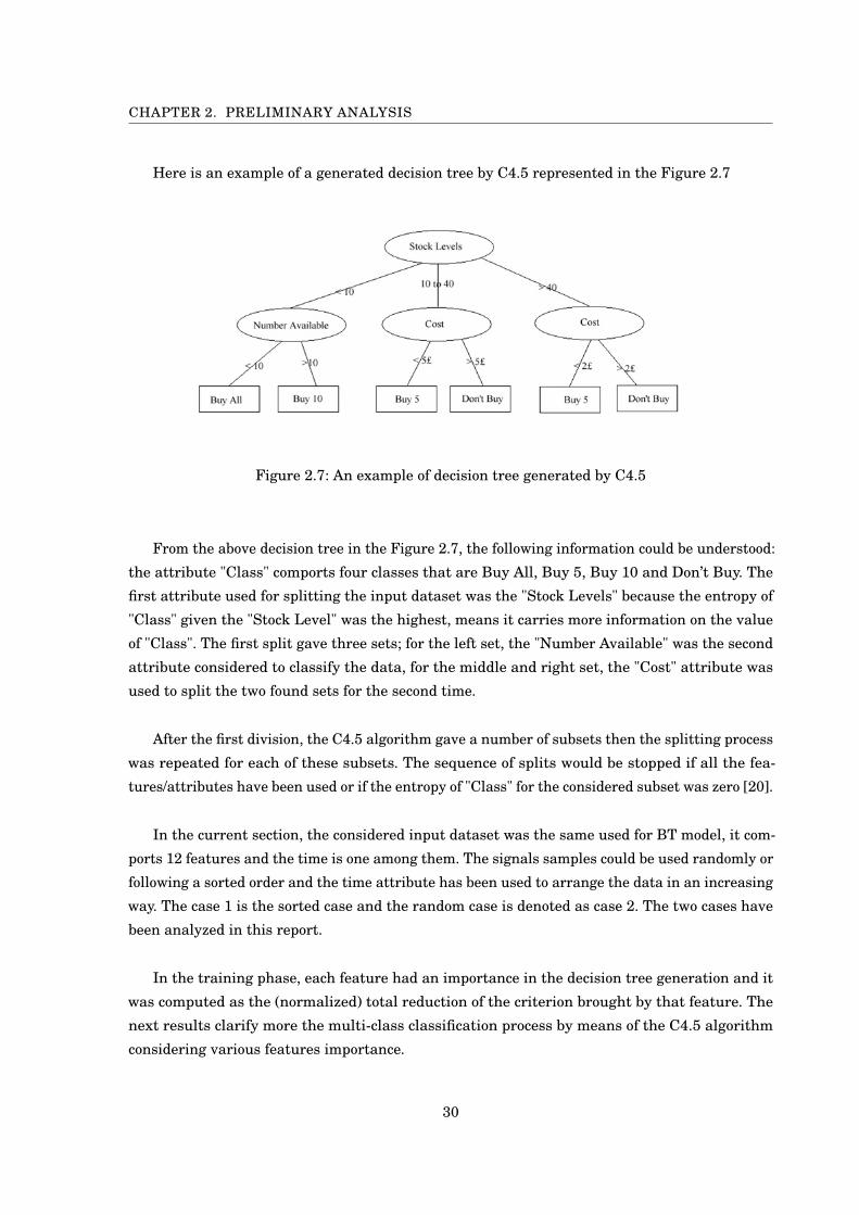
CHAPTER 2. PRELIMINARY ANALYSIS
Here is an example of a generated decision tree by C4.5 represented in the Figure 2.7
Figure 2.7: An example of decision tree generated by C4.5
From the above decision tree in the Figure 2.7, the following information could be understood:
the attribute "Class" comports four classes that are Buy All, Buy 5, Buy 10 and Don’t Buy. The
first attribute used for splitting the input dataset was the "Stock Levels" because the entropy of
"Class" given the "Stock Level" was the highest, means it carries more information on the value
of "Class". The first split gave three sets; for the left set, the "Number Available" was the second
attribute considered to classify the data, for the middle and right set, the "Cost" attribute was
used to split the two found sets for the second time.
After the first division, the C4.5 algorithm gave a number of subsets then the splitting process
was repeated for each of these subsets. The sequence of splits would be stopped if all the fea-
tures/attributes have been used or if the entropy of "Class" for the considered subset was zero [20].
In the current section, the considered input dataset was the same used for BT model, it com-
ports 12 features and the time is one among them. The signals samples could be used randomly or
following a sorted order and the time attribute has been used to arrange the data in an increasing
way. The case 1 is the sorted case and the random case is denoted as case 2. The two cases have
been analyzed in this report.
In the training phase, each feature had an importance in the decision tree generation and it
was computed as the (normalized) total reduction of the criterion brought by that feature. The
next results clarify more the multi-class classification process by means of the C4.5 algorithm
considering various features importance.
30

2.3. MULTICLASS CLASSIFICATION ALGORITHMS:
First of all, the Figure 2.8 resumes the whole process and identifies the different realized
steps, the description of those details is in the appendix at the end of this report.
Figure 2.8: Diagram flow of the C4.5 algorithm
2.3.3.1 Case 1: Sorted data
In this case, it is necessary to ensure that all the classes are included in the training data. That’s
why 80% of the total data was dedicated to the training phase while the rest was devoted to the
validation step. Unfortunately, with this condition the class 2 (moderate scintillation) was not
included in the testing phase while a few cases of class 4 (multipath) were present in the training
data.
The Figure 2.9 indentifies how the features were considered in the classification decision.
The six most important features were respectively time, φ60 (σφ), satellite ID, satellite azimuth,
C/N0, Satellite elevation.
31

CHAPTER 2. PRELIMINARY ANALYSIS
Figure 2.9: C4.5 features importances in the classification process when the data was sorted
It was impossible to include the obtained tree, in this report, because it was a huge and a
complex one. The obtained testing accuracy was 77% while the training accuracy was equal to
100%. It is clear that the classification performance was weak and an overfitting phenomenon
had occured due to the bad selection of the data sizes.
2.3.3.2 Case 2: Random data
The case 2 consists on shuffling the data samples before splitting it into two sets. Here, the same
data sizes, as the case 1, for training and testing sets have been used 80% and 20%, respectively.
Results are slightly improved as it is pointed in the Figure 2.10.
Figure 2.10: C4.5 features importances in the classification process when the data was random
32

2.3. MULTICLASS CLASSIFICATION ALGORITHMS:
Actually, the six most important features are respectively: time, φ60 (σφ), satellite ID, satellite
azimuth, C/N0 and S4RAW. The unique change was that the Satellite elevation was transformed
to S4RAW. The algorithm has given 100% training accuracy, the Minimum Square Error (MSE)
was 0 and 99% testing accuracy, the MSE was 0.06.
The Table 2.5 was inserted to compare the features importance, in the classification decision,
for both cases considering the same training and testing data sizes, 80% and 20%, respectively.
Feature Case 1: Sorted data Case 2: Random data
S4 0.002 0.006S4RAW 0.01 0.003
Satellite azimuth 0.15 0.16Satellite elevation 0.02 0.06
φ60 0.26 0.24φ30 0.001 0.002φ10 0.005 0.06φ3 0.0002 0.003φ1 0.002 0.004
time 0.27 0.29C/N0 0.05 0.04
Satellite ID (PRN) 0.23 0.18
Table 2.5: Comparaison between the classification importance of the considered features in case 1(sorted data) and case 2 (random data)
The Table 2.5 indicates that moving from the sorted case to the random case, the S4, S4RAW,
azimuth, elevation, φ10, φ3, φ1 and the time importances, in the classification process, have
raised while for the rest, the contrary.
The next analysis, in this thesis, will be performed upon the random case because it is more
generalized case. Besides, it is clear from the Table 2.5 and the previous two figures 2.9 and 2.10
that the classification decision was strongly based on the attribute/feature time, which has the
highest importance. The question is what would happen if the feature time is deletedfrom the observation matrix?
Always 80% of total data was used for training stage and after removing the time from the
considered features set, the Table 2.6 has been used to illustrate the reached results and to
compare between the two cases: random and sorted.
33

CHAPTER 2. PRELIMINARY ANALYSIS
Feature Case 1: Sorted data Case 2: Random data
W/o time W/ time W/o time W/ timeS4 0.01 0.002 0.01 0.006
S4RAW 0.038 0.1 0.035 0.003Satellite azimuth 0.18 0.15 0.2 0.16Satellite elevation 0.04 0.02 0.06 0.06
φ60 0.3 0.26 0.28 0.24φ30 0.02 0.001 0.005 0.002φ10 0.01 0.005 0.02 0.06φ3 0.01 0.0002 0.01 0.003φ1 0.01 0.002 0.01 0.004
time ; 0.27 ; 0.29C/N0 0.08 0.05 0.07 0.04
Satellite ID (PRN) 0.29 0.23 0.29 0.18
Table 2.6: Comparaison between the classification importance of the considered features in case 1(sorted data) and case 2 (random data) with and without the time attribute integration
The Table 2.6 confirms that the remained features importances, in the classification decision,
have raised with excluding the time attribute from the addressed set. In fact, their importances
have been enlarged because the decision was more based on them. The most important feature
became φ60. This result was expected because the ionospheric scintillation events are highly cor-
related with the time. Therefore, in cases when the time is included, it has the highest importance.
In addition, the importance values depend on the training data size. If the random case was
inspected, features importance vary with changing the considered training sizes from 80% to
50%. The Table 2.7 presents obtained results.
34

2.3. MULTICLASS CLASSIFICATION ALGORITHMS:
Feature Case 2.1: 80% training data size Case 2.2: 50% training data size
S4 0.006 0.006S4RAW 0.003 0.04
Satellite azimuth 0.16 0.15Satellite elevation 0.06 0.03
φ60 0.24 0.23φ30 0.002 0.009φ10 0.06 0.017φ3 0.003 0.004φ1 0.004 0.002
time 0.29 0.28C/N0 0.04 0.05
Satellite ID (PRN) 0.18 0.17
Table 2.7: Comparaison between features importance in the classification process using randomdata case and different training data sizes
In both detailed cases, the training accuracy was 100% while the testing accuracy was equal
to 98% if the half of the data was dedicated to the training phase and it was equal to 100% if
80% of the total input data was used to generate the trained model. The lower was the training
data size, the lower was the testing accuracy because the obtained model has been trained with
smaller number of cases.
Selecting the random case with employing 50% of the total data in the training step, it was
essential to verify whether the generated model has been overfitted or not. In case yes, it was
important to study how this phenomenon could be avoided.
The C4.5 algorithm outcome is a signle decision tree generated by the help of a nonparametric
model. This type of models is very flexible and is subject to overfit the training data. Each ML
algorithm includes many parameters and implements some techniques to limit the apparition of
overfitting and underfitting phenomena. Yet, overfitting is very difficult to be detected in practice
while underfitting is not the case, especially with a good evaluation metric.
The parameters affecting algorithm’s ability to conveniently modeling the given data are
called tuning parameters. It is necessary to correctly select them to optimize the classification
performance and to avoid misfit phenomena. For the C4.5, they are the following: the maximum
depth, the minimum number of samples per internal node, the minimum number of samples per
leaf node and the maximum number of considered features.
35

CHAPTER 2. PRELIMINARY ANALYSIS
The maximum depth: this parameter indicates the depth of the obtained decision tree. The
deeper is the tree, the larger is the number of nodes and splits. Generally, if this parameter is not
fixed the overfitting occurs and all nodes are expanded until all leaves are pure. A pure leaf is the
one composed by only positive cases confirming the chosen decision.
Figure 2.11: C4.5 training and testing accuracies as function of decision tree depth
In the Figure 2.11, fitting a decision tree with depths within the range of 1 to 32 has been
accomplished. Then the training and the testing performances were plotted to select the optimum
value of the maximum depth. From the Figure 2.11, it is clear that the tree depth does not affect
the model performance because no large difference, between illustrated accuracies, was present
whatever was the max depth value.
The minimum number of samples per internal node: it indicates the minimum number
of samples required to split an internal node. In the Figure 2.12, its minimum value was 1
sample per node and the maximum was considering all the samples at each node. Therefore,
this parameter was varied from 1% to 100% and the same as before the training and the testing
accuracies were plotted. The greater was this parameter, the more constrained was the obtained
tree.
The Figure 2.12 proves how increasing the minimum number of samples per internal node
leads to underfitting and especially considering 100% of the samples.
36

2.3. MULTICLASS CLASSIFICATION ALGORITHMS:
Figure 2.12: C4.5 training and testing accuracies as function of minimum number of samples perinternal node
The minimum number of samples per leaf node: it is very similar to the previous pa-
rameter and it denotes the minimum number of samples required to form a leaf node. The leaf
nodes are those at the base or the last level of the tree. The Figure 2.13 illustrates how both
training and testing accuracies are minimized when this parameter increases.
The same interpretations as the previous parameter the larger was this value, the lower was
the accuracy and it has extended underfitting.
Figure 2.13: C4.5 training and testing accuracies as function of minimum number of samples perleaf node
37

CHAPTER 2. PRELIMINARY ANALYSIS
The maximum number of features: it marks the maximum number of features to con-
sider during selecting the best split for an internal node. The Figure 2.14 displays the accuracy
variations responding to the changes of the considered features number.
Figure 2.14: C4.5 training and testing accuracies as function of features maximum number
In the Figure 2.14, it is shown that the testing accuracy was improved as the number of
considered features, in the splitting task, has gotten larger. The training accuracy was always
equal to 100%. According to the sklearn documentation, it is possible to consider more than the
maximum number of features to find a valid split of node samples.
In this work, the considered value for each of the previous parameters was the default one
that corresponds to the following: the minimum samples to split an internal node was set to
0.015%, the minimum samples per leaf node was set to 0.075% of total input data and the total
number of features was considered as the maximum features, which was 12.
Briefly, the previously mentioned values 100% and 98% representing training and testing
accuracies, respectively, has no overfitting or underfitting. The average 5-fold cross validation
testing accuracy that was higher than the average 5-fold cross validation training accuracy
confirms the absence of overfitting.
In the next chapter, it was better to consider the random case because the sorted one has
offered bad results and it did not allow to get the confusion matrix, except when 80% of all the data
was applied to train the model. In addition, this work aims to evaluate the classification outcome
by means of ML algorithms when training and testing phases have equivalent or unbalanced
dataset sizes.
38

2.3. MULTICLASS CLASSIFICATION ALGORITHMS:
2.3.4 Neural Network
The Neural Network (NN) or more precisely the Artificial Neural Network (ANN) is derived
from the human brain biological neural network [2]. The structure resemblance between them is
emphasised in the Figure 2.15.
Figure 2.15: The artificial neuron structure versus the brain neuron structure
The NN is useful to solve both regression and classification problems [4]. It is characterized
by its adaptive structure that could be updated based on the input data and the target outputs [4].
The designer chooses the structure to be implemented in the artificial network, specifies the
input and the outputs [4]. Every structure comports the input, the output and the hidden layers.
Each layer has a certain number of hidden nodes, called neurons, where any of them is identified
by its activation function [2]. The Figure 2.16 clarifies more the network design.
Figure 2.16: The ANN architecture
39

CHAPTER 2. PRELIMINARY ANALYSIS
In the Figure 2.16, each circle corresponds to a neuron or an activation function and the links
represent the connection weights that were optimized during the learning phase. Besides to the
weights, other variables, called biases, were optimized according to the inputs and the desired
outputs of the utilized network [4].
In this section, a multiclass classification was accomplished using NN structure generated
by python TensorFlow (TF). The TF is an open source ML library, contains many already imple-
mented algorithms. It has been developed by Google and it was released in October 2015. It offers
APIs in python or C++ and it is a powerful tool for either experts or beginners to develop several
applications for web, desktop or mobile [10].
The Gradient Descent algorithm, which is an iterative solution, has been used to optimize
the weights and biases. This algorithm is characterized by its initial learning coefficient that
must be chosen conveniently otherwise an overfitting or an underfitting could appear. Thus, it
is recommended to learn how to deal with these two phenomena. Underfitting comes when still
possible improvements on the testing data while overfitting is noticed if performances on testing
data are poorer than the ones on training set.
Equally, the NN is a supervised learning approach where the given dataset must be divided
into training and testing sets. The input dataset is the same of previous two sections and it was
used only with random data case.
In this elaborated thesis, the adopted NN framework includes one layer of each type: input,
hidden and output. This architecture has been utilized because for most NN classification prob-
lems, one hidden layer is completely enough to reach the target goal where input and output
layers are essential. For the input layer, neurons number was equal to the number of features or
columns in the observation matrix plus an additional single node identifying the bias term. For
the output layer, the softmax function has been used as activation function and the number of
output nodes was equal to the number of considered classes in the model. For the single hidden
layer, its neurons number was set to the mean of nodes existing in the input and the output layers .
For more details about the different steps of this approach, the flow diagram is illustrated in
the Figure 2.17. A detailed description about this flow was attached in the appendix at the end of
this report.
40

2.3. MULTICLASS CLASSIFICATION ALGORITHMS:
Figure 2.17: Diagram flow of the NN (TF) algorithm
To choose the optimum learning coefficient, the Table 2.8 has been used where three values of
the initial learning rate: 10−3, 10−4, 10−5 have been tested on the provided training dataset. The
one with the highest training accuracy would be selected in the coming analysis.
41

CHAPTER 2. PRELIMINARY ANALYSIS
Number of iteration 10−3 10−4 10−5
100 0.684 0.778 0.684200 0.684 0.816 0.71300 0.684 0.86 0.747400 0.684 0.86 0.76500 0.684 0.876 0.768600 0.684 0.883 0.771700 0.684 0.888 0.776800 0.684 0.902 0.785900 0.684 0.871 0.79
1000 0.684 0.907 0.7961100 0.684 0.896 0.8011200 0.684 0.922 0.8081300 0.684 0.925 0.8151400 0.684 0.918 0.8171500 0.684 0.926 0.821
Table 2.8: Training accuracies adopting different initial learning coefficients and iterationsnumber of the Gradient Descent
It was better to transform the presented data, in the Table 2.8, into the Figure 2.18 to clarify
more the appropriate choice for this coefficient.
Figure 2.18: NN training accuracies with devoting 50% of total data to training phase andconsidering various learning coefficients for the Gradient Descent algorithm
42

2.3. MULTICLASS CLASSIFICATION ALGORITHMS:
From the Figure 2.18, the best training performance was given by the 10−4 initial learning
rate. Besides to that, if the training data size has been enlarged to 80% of total provided data,
again the 10−4 gave the highest training accuracy. Therefore, it was selected for the next analysis
and processing phases.
In the other side, to identify the iterations number applied by the Gradient Descent to reach
the optimized weights and biases, a comparative study between training and testing accuracies
was accomplished. In fact, the Table 2.9 presents this comparison using various dataset sizes for
both ML stages.
43

CHAPTER 2. PRELIMINARY ANALYSIS
Number of iteration Training Testing50 % 80 % 50 % 20 %
100 0.778 0.787 0.773 0.788200 0.816 0.821 0.816 0.818300 0.86 0.844 0.855 0.845400 0.86 0.881 0.858 0.882500 0.876 0.891 0.868 0.893600 0.883 0.909 0.877 0.911700 0.888 0.919 0.882 0.916800 0.902 0.919 0.895 0.919900 0.871 0.923 0.859 0.9191000 0.907 0.929 0.893 0.9271100 0.896 0.918 0.882 0.9131200 0.922 0.935 0.913 0.9321300 0.925 0.943 0.913 0.9391400 0.918 0.902 0.91 0.9081500 0.926 0.937 0.913 0.9341600 0.935 0.935 0.922 0.9371700 0.934 0.946 0.924 0.9451800 0.938 0.949 0.931 0.9481900 0.942 0.951 0.932 0.9522000 0.93 0.937 0.927 0.9452100 0.94 0.95 0.936 0.952200 0.941 0.945 0.926 0.9472300 0.955 0.914 0.939 0.9112400 0.949 0.953 0.933 0.9532500 0.95 0.957 0.935 0.9592600 0.949 0.955 0.933 0.9542700 0.903 0.952 0.894 0.9552800 0.951 0.951 0.936 0.9472900 0.944 0.923 0.93 0.9323000 0.958 0.949 0.942 0.9493100 0.957 0.958 0.939 0.9583200 0.957 0.958 0.942 0.9563300 0.953 0.959 0.937 0.9583400 0.958 0.961 0.945 0.9593500 0.946 0.959 0.929 0.9573600 0.959 0.963 0.944 0.9643700 0.96 0.959 0.946 0.9583800 0.958 0.958 0.941 0.9563900 0.958 0.943 0.943 0.9454000 0.948 0.964 0.936 0.962
Table 2.9: Testing and training accuracies considering 10−4 as initial learning coefficient withvarious training data sizes
44

2.3. MULTICLASS CLASSIFICATION ALGORITHMS:
Logically, each model performs better on the training set since all the data are already seen
but a good model should be able to generalize well on unseen data and to reduce the gap between
performances on training and testing sets. The testing accuracy, presented in the Table 2.9, was
obtained using the optimum weights and biases found at the end of the training phase.
From the Table 2.9, it is clear that the Gradient Descent iterations number depends on the
dataset size. Using 4000 iterations to select the optimum number, was more than enough because
the accuracies were almost constant after iteration number 3000.
From the Table 2.9 and the Figure 2.19, it is visible that the testing accuracy, called also a
validation accuracy, was following the training accuracy quite closely, which means no overfitting
is present and the gap between training and testing accuracies is very feeble. NNs tend to perform
overfitting when they have adequate performance on the training data whereas they do not adapt
very well to the testing data.
Besides, overfitting gets higher if the number of parameters, e.g the number of hidden layers
and the number of neurons increases because more degrees of freedom are present and the NN
learns too much the training data. The number of iterations must be minimized as much as
possible otherwise, the process will be expensive in terms of training time.
Figure 2.19: NN training and testing accuracies with devoting 50% of total input data for eachphase
For the case when 80% of total input data was integrated to generate the trained model, the
Figure 2.20 was advantageous to fix the Gradient Descent iterations number.
45

CHAPTER 2. PRELIMINARY ANALYSIS
Figure 2.20: NN training and testing accuracies with devoting 80% of total input data for eachphase
From the Figure 2.19, the optimum iterations number was 3700 because it gave the highest
training and testing accuracies, 96% and 94.6%, respectively. From the Figure 2.20, the optimum
iterations number was 3600, which gave a performance value equal to 96.3% and 96.4% for
training and testing phases, respectively.
Conclusion
This chapter was dedicated to perform a comparative study between various existing ML algo-
rithms for classification and based on their performances over the provided dataset, three among
them have been selected. The three selected algorithms were BT, NN (TF) and C4.5. The next
chapter aims to highlight and to compare the results of automatic scintillation identification and
detection outcomes considering two features sets in the input data. The first set was based on
amplitude or phase scintillation indices absolute values while the second one was based on the
frequency domain features.
46

CH
AP
TE
R
3RESULTS AND DISCUSSION
Introduction
This chapter was devoted to discuss the automatic detection returns of ionospheric scin-
tillation via the previous three chosen classifiers. The opted systems evaluation was
accomplished via confronting their performances in terms of accuracies and confusion
matrices. Indeed, two different features sets have been used to produce this work. Consequently,
this chapter was divided into two main parts. The first part emphasizes how the absolute values
of amplitude and phase fluctations indices, S4 and φ60, were used in the detection process while
the second part, confirms the effectiveness of frequency domain features in giving a more reliable
distinction.
3.1 Ionospheric scintillation automatic detection based onabsolute values of scintillation indicators S4 and φ60
First of all, the code devlopped during this work in both softwares, MATLAB and Spyder
(PYTHON), must give the same results each time scripts will be executed otherwise, the compari-
son is useless. More than that, to compare two confusion matrices or two accuracies values, it is
important to create the same environement such as data sizes, accuracy expression etc.
The current section presents the adopted algorithms’ outcome over the first set of GPS L1C/A
data that contains low rate samples. Each sample was formed by 12 features plus a class label,
which are shown in the Figure 3.1. Among the 12 features, there were the absolute values of S4
and φ60 with the time expressed in seconds and the C/N0 expressed in dB-Hz etc.
47

CHAPTER 3. RESULTS AND DISCUSSION
Figure 3.1: The first set of employed features, in the elaborated work, based on the absolutevalues of S4 and φ60 measurements
The Table 3.1, outlines the number of cases for each class in the first input data:
Scintillation class 0 (None) 1 (Low) 2 (Moderate) 3 (Strong) 11/4 (Multipath)
Cases number 9117 1684 1261 765 499
Table 3.1: Number of cases identifying each class, in the first input dataset, based on absolutevalues of scintillations indicators, S4 and φ60
In view of various training data sizes, the Table 3.2 was used to resume the classification
achievements in terms of testing and training accuracies. As it was mentioned, the considered
accuracy expression must be the same for the three executed methods.
NN (TF) DT (C4.5 ) BT
Training data size 50% 80% 50% 80% 50% 80%
Training (%) 95.96 96.31 100 100 96.9 97.8Testing (%) 94.63 96.36 97.57 98.65 97.66 98.4
Table 3.2: Testing and training accuracies considering input data based on absolute values ofscintillation indicators, S4 and φ60, with various training dataset sizes for the three selectedmethods
The implemented accuracy expression by the three approaches; BT, C4.5 and NN consists on
computing the fraction of correctly classified samples, means the sum of correctly predicted labels
divided by the total number of samples. The next expression explains more how the accuracy was
calculated:
(3.1)NX
n=11{LabelTrue = LabelPredicted}
48

3.1. IONOSPHERIC SCINTILLATION AUTOMATIC DETECTION BASED ON ABSOLUTEVALUES OF SCINTILLATION INDICATORS S4 AND φ60
However, the accuracy related to any class consists on calculating the number of correctly pre-
dicted samples of that class then dividing them by the total number of true cases identifying the
mentioned class in the input dataset.
From the Table 3.2, it is understandable that no overfitting was present because the difference
between testing and training accuracies values was very low. In addition, the highest training
performance was offered by the C4.5 decision tree followed by the BT and the NN, respectively.
The outcomes similarities between the C4.5 and the BT is due to the resemblance in the
decision process realized by them. Both of them are based on a tree-like model to make the
decision. The C4.5 generates a signle decision tree while the BT algorithm is based on generating
many decision trees and ending with averaging all the predictions given by them. In addition, the
C4.5 is stronger in handling missing values with both continuous and discrete attributes than
BT. That’s why it had a result slightly better than BT
The accuracy is a generalized metric to evaluate the robustness of any ML algorithm while
the confusion matrix is a more precise performance metric because it measures the classification
or the prediction accuracy realted to each class. As well, it measures the true positive and the
true negative rates as it was mentioned in the previous chapter.
The coming parts of this section, aim to compare between the testing and the training
confusion matrices for the same algorithm then comparing the three obtained testing confusion
matrices between them. In addition, a comparative study for the misclassification outcome will
be addressed.
3.1.1 Bagged Trees
As it was indicated earlier, the analysis and the studies would be concerning the confusion matrix
obtained after activating the 5-fold cross validation technique. This matrix, which is shown in the
Figure 3.2 (a), has been already introduced in the chapter 2 but it was shown with the numbers
of correctly and incorrectly predicted values and not in percentage (%). Here it is presented in
percentage to ease drawing an analogy between the three opted classifiers.
49

CHAPTER 3. RESULTS AND DISCUSSION
(a) (b)
Figure 3.2: The BT confusion matrices obtained after activating the 5-fold cross validationtechnique considering 50% of input dataset during training phase: (a) Training, (b) Testing
From the Figure 3.2, it is clear that the BT classifier had a good performance for both training
and testing sets. Obviously, all the estimation percentages were higher than 85% and this is owing
to the robustness of BT algorithm, which is based on averaging the generated trees ensemble. In
the testing phase, the prediction findings were slightly better than training results except for the
class 11 (multipath) and class 2 (moderate).
In both matrices, the highest accuracy value was given by the class 0 (non scintillation),
the second value was given by the class 1 (low scintillation) and the lowest value was given by
the multipath class. This nethermost performances, of class 11, are due to the lower number
of trained multipath cases while the uppermost accuracies, of the class 0, are due to the larger
number of its trained cases.
In addition, the largest misclassification value was between class 0 and class 4. For both
training and testing stages, 13% was the value of wrongly predicted cases as class 0 while in
reality they are of class 11. This ambiguity was provoked because multipath class was not well
trained. Further, the misclassification rate between scintillation classes; 1, 2 and 3 was a bit high.
For example, 5% to 6% of strong scintillation cases were misdetected as low scintillation and the
misdetection between moderate and strong or low scintillation was around 2% to 5%.
Other important information that could be read out from the Figure 3.2, is that almost no
misclassifications between multipath and scintillation classes were present. On the other side,
50
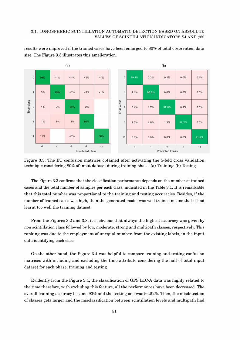
3.1. IONOSPHERIC SCINTILLATION AUTOMATIC DETECTION BASED ON ABSOLUTEVALUES OF SCINTILLATION INDICATORS S4 AND φ60
results were improved if the trained cases have been enlarged to 80% of total observation data
size. The Figure 3.3 illustrates this amelioration.
(a) (b)
Figure 3.3: The BT confusion matrices obtained after activating the 5-fold cross validationtechnique considering 80% of input dataset during training phase: (a) Training, (b) Testing
The Figure 3.3 confirms that the classification performance depends on the number of trained
cases and the total number of samples per each class, indicated in the Table 3.1. It is remarkable
that this total number was proportional to the training and testing accuracies. Besides, if the
number of trained cases was high, than the generated model was well trained means that it had
learnt too well the training dataset.
From the Figures 3.2 and 3.3, it is obvious that always the highest accuracy was given by
non scintillation class followed by low, moderate, strong and multipath classes, respectively. This
ranking was due to the employment of unequal number, from the existing labels, in the input
data identifying each class.
On the other hand, the Figure 3.4 was helpful to compare training and testing confusion
matrices with including and excluding the time attribute considering the half of total input
dataset for each phase, training and testing.
Evidently from the Figure 3.4, the classification of GPS L1C/A data was highly related to
the time therefore, with excluding this feature, all the performances have been decreased. The
overall training accuracy became 93% and the testing one was 94.52%. Then, the misdetection
of classes gets larger and the misclassification between scintillation levels and multipath had
51

CHAPTER 3. RESULTS AND DISCUSSION
occured. Moreover, it is visible that the classes most correlated to the time feature were low
scintillation (class 1) and multipath (class 2).
(a) (b)
(c) (d)
Figure 3.4: The obtained BT confusion matrices considering 50% of dataset size in the trainingstage with and without the time attribute integration in the features set: (a) Training CM withtime , (b) Training CM without time, (c) Testing CM with time, (d) Testing CM without time
52

3.1. IONOSPHERIC SCINTILLATION AUTOMATIC DETECTION BASED ON ABSOLUTEVALUES OF SCINTILLATION INDICATORS S4 AND φ60
3.1.2 C4.5 Decision Tree
In the current section, the multipath class was denoted as 4 and not 11. Then, as it was specified
in the previous chapter, the provided dataset could be, based on the time attribute, sorted in
increasing order or not. Performances in the sorted case were very poor and it was difficult to
get the confusion matrices at the end of the approach due to the hardness of including all the
existing classes in the testing and the training phases.
More precisely, given that the total number of data samples was 13326 and if 50% of them
was dedicated for training stage then, not all classes are included in both phases. The main
issue was with the class 2 (moderate scintillation) and the class 4 (multipath). It was difficult
to include both classes 2 and 4 together because the class 4 starts from the observation number
9338 while the class 2 ends in the observation number 8880. Therefore, only the random case
would be discussed in the current section.
The Figure 3.5 illustrates the training and the testing confusion matrices obtained via
executing the C4.5 algorithm over the random data with dedicating 50% of it to the training
stage.
(a) (b)
Figure 3.5: The obtained C4.5 confusion matrices considering 50% of total data in the trainingstage: (a) Training, (b) Testing
The same as BT, the Figure 3.5 demonstrates that all the classes have been perfectly predicted
in both phases where all accuracies were above 85%. Then, the training reliability was higher
than the testing one for all the existing classes.
53

CHAPTER 3. RESULTS AND DISCUSSION
Furthermore, 100% was the training accuracy value for all the considered labels while for the
testing accuracy, the topmost value was given by non scintillation class followed by low, moderate
and strong classes, respectively. The smallest returns was given by multipath class due to its
elevated misclassification rate with non scintillation class, 14.5% of multipath cases have been
incorrectly classified as false negative.
More, almost no misclassifications between scintillation levels and multipath were present
means scintillation cases were well trained by the produced model. Equally, 0% of cases from
moderate class have been wrongly detected as non scintillation. For the strong cases, the detection
disruptions with low cases were higher than its misclassification rate with the moderate cases.
If the training data portion was increased from 50% to 80% of total input data, the testing
matrix content has been changed. The Figure 3.6 shows this change and illustrates the distinction
between the two tested cases; 80% and 50%.
(a) (b)
Figure 3.6: The obtained C4.5 testing confusion matrices considering different training datasetsizes : (a) 50% of total input data for training, (b) 80% of total input data for training
From the Figure 3.6, it is understandable that the larger was the training dataset size, the
lower was the classification error because when a high number of cases were trained then the
probability of finding a new case during testing stage is poor. For example, the misclassification
of class 4 as class 0 was reduced from 14.5% to 0.93% while the misclassification of class 4 as
class 1 was withdrawn. The same for the overall misclassification, which was decreased from
2.43% to 1.35%.
54

3.1. IONOSPHERIC SCINTILLATION AUTOMATIC DETECTION BASED ON ABSOLUTEVALUES OF SCINTILLATION INDICATORS S4 AND φ60
It was not important to cite the training confusion matrix because even if 80% of data was
used to train the model, the training accuracy remained always 100% while the overall testing
accuracy was enlarged to 98.65%.
In the other side, with removing the time attribute from the observation data and performing
the classification process by the help of the remained 11 features considering dissimilar training
data sizes, the obtained testing confusion matrix are illustrated in the Figure 3.7.
(a) (b)
Figure 3.7: The C4.5 Testing confusion matrices with excluding the time feature and withconsidering different training dataset sizes: (a) 50% of total data for training, (b) 80% of totaldata for training
Comparing the Figure 3.7 to the Figure 3.6 confirms that removing the time from the re-
maind features provokes the overall accuracy mitigation. This reduction was due to the higher
correlation value between the time attribute and the ionospheric scintillation apparition.
Besides, the classification error was enlarged. For example; if 50% of samples has been dedi-
cated to train the model and with including the time attribute, the misclassification of class 4 as
class 0 was equal to 14.5% while if the time has been deleted from the features set, this error
became 17.65%. For the 80% case, if the time was excluded then the error has been raised from
0.93% to 7.48%.
55

CHAPTER 3. RESULTS AND DISCUSSION
With enlarging the training data from 50% of total samples to 80%, the overall testing
accuracy was augmented from 93.8% to 96.06%. On the contrary, the misclassification has been
decreased. Using 50%, of total input data, for training step and the 12 existing features gave
better results than using 80% of data with excluding the time attribute.
3.1.3 Neural Network
The NN was studied and was commented, only in the case when the data samples were randomly
inserted. This case was considered to avoid the same problem of classes integration with testing
dataset. The obtained training and testing confusion matrices, in case data sizes were equal for
both phases, are displayed in the Figure 3.8:
(a) (b)
Figure 3.8: The obtained training and testing NN confusion matrices in case 50% of total inputdata was used to train the model : (a) Training, (b) Testing
From the Figure 3.8, it is deduced that the overall classification performance produced by
NN was comaparable to previous approaches; C4.5 and BT. As well as, it is apparent that NN
performance was better over training data than over the testing one. Equally to the chosen
decision trees classifier systems, highest training and testing accuracies were given by the class
0 (non scintillation) and they were 99.47% and 99.21%, respectively.
The same as BT and C4.5, the multipath class was never wrongly predicted as a scintillation
case; low, moderate or strong. However, misclassification percentage between two successive
classes, such as classes 1 and 2 or 2 and 3 was within the range of 6% to 18%. The NN was
not able enough to well distinguish strong scintillation level and multipath because it gave the
56
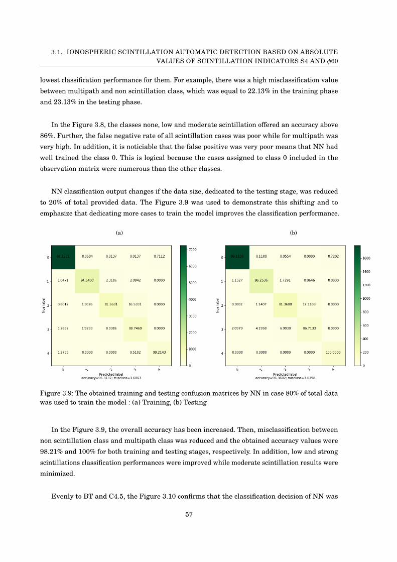
3.1. IONOSPHERIC SCINTILLATION AUTOMATIC DETECTION BASED ON ABSOLUTEVALUES OF SCINTILLATION INDICATORS S4 AND φ60
lowest classification performance for them. For example, there was a high misclassification value
between multipath and non scintillation class, which was equal to 22.13% in the training phase
and 23.13% in the testing phase.
In the Figure 3.8, the classes none, low and moderate scintillation offered an accuracy above
86%. Further, the false negative rate of all scintillation cases was poor while for multipath was
very high. In addition, it is noticiable that the false positive was very poor means that NN had
well trained the class 0. This is logical because the cases assigned to class 0 included in the
observation matrix were numerous than the other classes.
NN classification output changes if the data size, dedicated to the testing stage, was reduced
to 20% of total provided data. The Figure 3.9 was used to demonstrate this shifting and to
emphasize that dedicating more cases to train the model improves the classification performance.
(a) (b)
Figure 3.9: The obtained training and testing confusion matrices by NN in case 80% of total datawas used to train the model : (a) Training, (b) Testing
In the Figure 3.9, the overall accuracy has been increased. Then, misclassification between
non scintillation class and multipath class was reduced and the obtained accuracy values were
98.21% and 100% for both training and testing stages, respectively. In addition, low and strong
scintillations classification performances were improved while moderate scintillation results were
minimized.
Evenly to BT and C4.5, the Figure 3.10 confirms that the classification decision of NN was
57

CHAPTER 3. RESULTS AND DISCUSSION
strongly based on the time feature. That’s why after deleting the time from the set of considered
features, all the prediction metrics have been decreased and especially the one related to low
scintillation class. For example the testing accuracy of class 1 was 71.05%, in the Figure 3.10 (c),
when the time feature was included but it has scaled down to 69.76%, in the Figure 3.10 (d), with
excluding the time.
(a) (b)
(c) (d)
Figure 3.10: The obtained NN confusion matrices considering 50% of total input dataset sizein the training stage with and without the time attribute integration in the features set: (a)Training CM with time , (b) Training CM without time, (c) Testing CM with time, (d) Testing CMwithout time
58

3.1. IONOSPHERIC SCINTILLATION AUTOMATIC DETECTION BASED ON ABSOLUTEVALUES OF SCINTILLATION INDICATORS S4 AND φ60
More precisely, the misclassification between multipath and low/moderate scintillation had
appeared and the false negative rate, for all classes, had augmented except for multipath it had
diminished. The highest misclassification value was given by the low scintillation cases that were
wrongly predicted as non scintillation cases with a percentage equal to 26.70% and 26.73% for
training and testing accuracy, respectively.
From the Figure 3.10, it is observable that the misclassification between consecutive classes,
like 1 and 2 or 2 and 3, had grown. Besides, the events detected incorrectly as strong scintillation
while their real class were low or moderate scintillation has been increased. In this context, the
precise detection and identification of scintillation events was highly combined with time feature.
3.1.4 Conclusions in this study
Through applying the BT, C4.5 and NN algorithms over a low rate GPS L1C/A data, gathered by
commercial ISM receiver in the Antarctica continent, in the purpose of performing automatic
detection for scintillation levels or multipath events, the next significant points were gained:
• All overall accuracies were good and were above almost 95%.
• Attained performances depend on the total number of samples per each class included in
the input dataset and used during training phase.
• Enlarging the number of trained cases, better performances were reached for all considered
algorithms.
• If the half of input data was used to generate and to train the classification model, the
highest accuracy was given by non scintillation class because it had the larger number of
observations in the input data while the lowest accuracy was presented by multipath.
• The classification outcomes were highly related to the existence of the time attribute among
the features set because performances have been decreased with excluding the time.
• The low scintillation and the multipath classes were strongly correlated to the time at-
tribute.
• Using the total number of provided features in the detection process, reveals a weak
misdetection of multipath as a scintillation case and vice versa.
The previous section was dedicated to discuss the results of the classification process based on the
absolute values of S4 and φ60 indicators representing the amplitude scintillation and the phase
fluctuation measurements, respectively [13], [12]. In generale, the performances were good, for
the three selected algorithms, because each of them gave an overall accuracy above 93% with and
59
CHAPTER 3. RESULTS AND DISCUSSION
without time integration. Dedicating more cases to generate the trained model was an optimum
choice for all the approaches.
Some previous studies in the field of ML application over GPS L1C/A data like in [13]
and [12] have presented the weakness of features containing S4 and φ60 in the detection and the
identification process. In fact, the set of picked features includes absolute values of scintillation
irregularities indicators, S4 and φ60, was not strong enough in the classification. This weakness
is because of ignoring the high-dimensional features like the frequency domain components in
making the decision [13].
3.2 Ionospheric scintillation automatic detection based on thefrequency domain features of scintillation indicators S4and φ60
Preceding researches, such as [13] and [15], have proved that using features in the frequency
domain like the PSD, was more robust in the classification operation, especially in distinguishing
scintillation phenomenon from other events like multipath and interference. In this section, a
second features set, based on frequency domain components, was used by the selected three
algorithms to autonomously detect amplitude or phase irregularities.
This set was already presented in the previous chapter. It contained S4/φ60, S4/φ60 maxi-
mum, S4/φ60 mean and the rest was dedicated to the PSD features calculated using the STFT
over a 3-min windows. To generate this observation data, the raw data files were used, which
were composed of data acquired during three consecutive days with a sampling rate equal to 50Hz.
The calculated input matrix had 3999 samples and each sample was assigned to a class label
following the hard method that consists on comparing either S4 or φ60 to predefined thresholds.
In this section, two cases have been discussed ; the first case aimed to study the algorithms’
robustness, in the amplitude scintillation detection, using PSD functions of S4, while the second
one was dedicated to discuss their robustness, in the phase scintillation prediction, via PSD func-
tions of φ60. The number of samples per each class had changed from the amplitude irregularities
detection case to the phase variations detection case, numbers are reported in the Table 3.3:
60

3.2. IONOSPHERIC SCINTILLATION AUTOMATIC DETECTION BASED ON THEFREQUENCY DOMAIN FEATURES OF SCINTILLATION INDICATORS S4 AND φ60
Scintillation class 0 (None) 1 (Low) 2 (Moderate) 3 (Strong)
Cases number (amplitude) 3192 506 146 155
Cases number (phase) 343 513 3143 0
Table 3.3: Samples number per each class in the second input dataset, which was based on thefrequency domain features of scintillation indicators, S4 or φ60, for both amplitude or phasescintillation detection cases
From the Table 3.3, it is visible the unbalance of observations numbers between classes in
both addressed cases. For the amplitude scintillation study, the none scintillation class had the
largest number of samples followed by low, strong and moderate scintillation, respectively. For
the phase scintillation study, most of cases were assigned to the moderate scintillation class
followed by low and none scintillation classes, respectively. However, zero case had identified the
strong scintillation class.
As it was already reported, the three chosen algorithms were based on a supervised learning
approach therefore, various training and testing datasets sizes have been considered. The perfor-
mance assessments and interpretations, related to the application of those three algorithms over
the obtained observation matrix, were divited into two parts. To perform outcomes comparison,
it was neccessary to consider the same conditions in terms of accuracy expression and training
dataset size.
The automatic detection of amplitude scintillation was accomplished through employing, in
the classification proces, GPS L1C/A data that contained only S4 and its studied PSD components.
The phase scintillation detection was based on the algorithms application over GPS L1C/A data
that contained only PSD components gathered from φ60.
3.2.1 Bagged Trees
The 5-fold cross validation technique was implemented as a model validation technique to avoid
overfitting phenomenon. The 25% holdout validation choice was discarded because it is more
suitable for large datasets while the input matrix had only 3999 samples. The next results were
obtained with dedicating the 80% of total data to the training step and the rest to the testing
stage.
3.2.1.1 Amplitude scintillation detection
The Figure 3.11 illustrates the obtained testing and training BT confusion matrices.
61

CHAPTER 3. RESULTS AND DISCUSSION
(a) (b)
Figure 3.11: The obtained BT training and testing confusion matrices considering 80% of thetotal input data based on S4 PSD components to train the model: (a) Training, (b) Testing
In the Figure 3.11, it is conspicuous the absence of multipath class. The presented outcomes,
over GPS high rate data, have been achieved using 3199 samples to generate the trained model
from a total of 3999 samples. The attained overall performance, for training and testing phases,
were 96.1% and 96.88%, respectively.
In the section 3.1.1, the gained overall BT accuracy, over GPS low rate data, was 97.8% for
the training phase and 98.4% for the testing stage. Those two values were reached via using 80%
of the total input data, which was equal to 10661 samples, during training phase. The absolute
value of S4 was among the parameters characterizing each observation of them.
Comparing the current obtained overall accuracies to 3.1.1 outcomes and taking into con-
siderations the difference between the considered training datasets sizes in both cases, the
performances were close enough and were comparable, which means the employed frequency
domain features were strong in the detection operation.
The Figure 3.11 reveals the absence of misclassification between non consecutive classes,
such as none and strong scintillation or low and strong scintillation. Their misclassification
rate was already null. In addition, the none scintillation class had offered the highest accuracy
for both stages means it was well trained. However, the largest training misclassification rate
was between moderate and low scintillations classes. In the training phase, 22% of moderate
cases have been wrongly classified as low cases and 14% of strong scintillation cases have been
62

3.2. IONOSPHERIC SCINTILLATION AUTOMATIC DETECTION BASED ON THEFREQUENCY DOMAIN FEATURES OF SCINTILLATION INDICATORS S4 AND φ60
incorrectly predicted as moderate cases. For the testing phase, the misclassification between
strong and moderate scintillation was higher than the one between low and moderate. In addition
to that, the strong scintillation class was better trained than the moderate one, which has given
the lowest training accuracy but in the testing phase, the moderate scintillation has presented a
greater accuracy.
The none scintillation class was well trained because it had the highest number of samples
in the input matrix. The low scintillation class gave the second highest accuracy because it had
the second largest number of samples in the input data. Consequently, the realized results are
logical with respect to the number of employed samples.
3.2.1.2 Phase scintillation detection
The Figure 3.12 displays the two obtained confusion matrices at the end of BT execution.
(a) (b)
Figure 3.12: The obtained BT training and testing confusion matrices considering 80% of thetotal input data based on φ60 PSD components to train the model: (a) Training, (b) Testing
As it was mentioned in the Table 3.3, the provided dataset did not contain any case identifying
strong phase scintillation, which corresponds to class 3. The reached global training accuracy
was 98.2% and the testing one was 99.13%. The Figure 3.12 emphasises that all classes have
presented an accuracy between 92% to 100% despite of the unbalance in the samples number
assigned to each class.
63

CHAPTER 3. RESULTS AND DISCUSSION
In the training phase, the moderate scintillation class has presented the largest accuracy,
which was greater than 99%, because of its higher trained cases number in the observation data.
In the testing phase, the misclassification between low and moderate scintillation was greater
than their misclassification with non scintillation. In addition, the given training accuracy values,
by the low and the non scintillation classes, were 92% and 96%, respectively. Those values were
comparable to the one already offered by class 2 despite the difference in the used samples
number identifying each class
From the Figure 3.12, it is remarkable that the employed data was adequate for the detection
process because of the gotten good performance. Well, the generated training model was vigorous
enough to classify the data correctly.
3.2.2 C4.5 Decision Tree
The same as previous section, two cases have been studied to discuss the automatic amplitude
and phase variations using the second input data with the C4.5 algorithm.
3.2.2.1 Amplitude scintillation detection
To be sure that no overfitting or underfitting was present, a short preliminary analysis has been
performed using the Figures 3.13, 3.14 and 3.15. The next analysis was used to optimize the
selection of tuning parameters, to enhance the scintillation events classification returns by the
C4.5 and to avoid overfitting occurrence. The studied parameters were : the maximum depth, the
minimum number of samples per internal node and the minimum number of samples per leaf
node.
The maximum depth: it was already pointed out that this parameter denotes the depth of
the decision tree and it is important to fix it to withdraw overfitting.
64

3.2. IONOSPHERIC SCINTILLATION AUTOMATIC DETECTION BASED ON THEFREQUENCY DOMAIN FEATURES OF SCINTILLATION INDICATORS S4 AND φ60
Figure 3.13: The C4.5 training and testing accuracies as function of decision tree depth considering80% of the total input data based on S4 PSD components
From the Figure 3.13, it is notable that no overfitting was present whatever was the tree
depth therefore, no need to fix it.
The minimum samples splits: it identifies the minimum number of samples required to
split an internal node within the tree.
Figure 3.14: The C4.5 training and testing accuracies as function of minimum number of samplesrequired to split an internal node considering 80% of the total input data based on S4 PSDcomponents
The minimum samples leafs: it references the minimum number of samples required to
form a leaf node, which is located at the decision tree basis.
65

CHAPTER 3. RESULTS AND DISCUSSION
Figure 3.15: The C4.5 training and testing accuracies as function of minimum number of samplesrequired to form a leaf node considering 80% of the total input data based on S4 PSD components
From the Figures 3.14 and 3.15, a good selection for minimum samples splits and minimum
samples leafs were 0.1 and 0.05, respectively. However, the obtained overall accuracy was 100%
for both training and testing phases whatever the considered training dataset sizes 60%, 80%
and 90% of total input data based on S4 PSD components. In case 80% was used to train the
model, the Figure 3.16 displays the confusion matrices calculated at the end of each step.
(a) (b)
Figure 3.16: The obtained C4.5 training and testing confusion matrices considering 80% of thetotal input data based on S4 PSD components to train the model: (a) Training, (b) Testing
66

3.2. IONOSPHERIC SCINTILLATION AUTOMATIC DETECTION BASED ON THEFREQUENCY DOMAIN FEATURES OF SCINTILLATION INDICATORS S4 AND φ60
From the Figure 3.16, it is evident that the C4.5 algorithm was powerful in the automatic
amplitude scintillation detection using the provided dataset regardless of the inequality between
number of samples for each class.
3.2.2.2 Phase scintillation detection
In the current part, the same preliminary analysis steps have been realized to optimize tuning
parameters choice and to appropriately fit the generated model. The C4.5 training and testing
accuracies as function of tree depth, minimum number of samples required to split an internal
node and minimum number of samples required to form a leaf node are represented in the
Figures 3.17, 3.18 and 3.19, respectively.
Considering 80% of the total input data based on φ60 PSD functions to train the model, the
next Figures 3.17, 3.18 and 3.19 were offered:
67

CHAPTER 3. RESULTS AND DISCUSSION
Figure 3.17: Training and testing accuracies as func-tion of tree depth
Figure 3.18: Training and testing accuracies as func-tion of minimum number of samples required tosplit an internal node
Figure 3.19: Training and testing accuracies as func-tion of minimum number of samples required toform a leaf node
Generally, the behaviors introduced in the Figures 3.17, 3.18 and 3.19 are similar to the
ones obtained during the amplitude scintillation detection and presented in the Figures 3.13,
3.14 and 3.15. Therefore, the same tuning parameters values have been chosen; the max depth
was not fixed, 0.1 and 0.05 were used for minimum samples splits and minimum samples leafs,
respectively.
Equally to previous part, considering various training dataset sizes that were 60%, 80%
and 90% gave the same outcome, which was 100% for both phases. It is evident the overfitting
phenomenon absence due to the null gap between training and testing accuracies. The computed
confusion matrices are represented in the Figure 3.20.
68

3.2. IONOSPHERIC SCINTILLATION AUTOMATIC DETECTION BASED ON THEFREQUENCY DOMAIN FEATURES OF SCINTILLATION INDICATORS S4 AND φ60
(a) (b)
Figure 3.20: The obtained C4.5 training and testing confusion matrices considering 80% oftotal input data based on φ60 PSD components to train the model and after fixing the tuningparameters: (a) Training, (b) Testing
In the Figure 3.20, both matrices have presented 100% as classification accuracy for all the
considered classes despite the unbalance between the existing samples per each class in the input
set. Certainly this perfect performance was due to the robustness of the C4.5 and the effectiveness
of the considered input matrix. Another reason behind the absence of misclassification could be
the usage of less classes where only three classes were used.
3.2.3 Neural Network
Equally in the current section, the adopted network structure was equivalent to the one used in
the first part of this thesis and the considered training dataset size was 80% of total input data
based on either S4 or φ60 PSD features. Before performing the classification of samples via the
network, it was essential to carry out some processing steps that aimed to select the optimum
initial learning rate of the Gradient Descent algorithm and the total number of training epochs
or iterations.
3.2.3.1 Amplitude scintillation detection
Analysing the behavior of the adopted structure over the selected data, the Figure 3.21 displays
the Gradient Descent performance comparison considering different learning coefficients. Initial
coefficients rate that are greater than 10−6 were discared because they have retrogressed the
classification returns.
69

CHAPTER 3. RESULTS AND DISCUSSION
Figure 3.21: The NN classification training accuracy versus Gradient Descent iterations numberwith adopting different initial learning coefficients over 80% of the provided data based on PSDcomponents, acquired from S4, to generate the trained model
From the Figure 3.21, it is clear that the training accuracy was constant with all the values
except when the initial learning rate was equal to 10−6 therefore, it has been selected for the next
analysis. The Figure 3.22 was auxiliary to determine the Gradient Descent iterations number.
Figure 3.22: NN training and testing accuracies with 80% of total PSD components, acquiredfrom S4, devoted for training phase and with initial learning rate equal to 10−6
The Figure 3.22, indicates that the highest testing accuracy was equal to 88.5% while for the
training phase the highest value was 90.6%. However, it is clear that no more improvements
were attained after iteration number 150 therefore, it has been chosen, as the Gradient Descent
iterations number, for the classification study. In addition, the overfitting phenomenon starts to
70

3.2. IONOSPHERIC SCINTILLATION AUTOMATIC DETECTION BASED ON THEFREQUENCY DOMAIN FEATURES OF SCINTILLATION INDICATORS S4 AND φ60
appear after iteration number 150.
The NN obtained confusion matrices are represented in the Figure 3.23:
(a) (b)
Figure 3.23: The NN obtained training and testing confusion matrices considering 80% of totalinput data based on S4 PSD features to train the model: (a) Training, (b) Testing
From the Figure 3.23, it is shown that the best performance was given by the non scintillation
class where 98.68% was the training accuracy and 96.88% was the testing one. In addition, the
training and testing performance were very poor over the moderate and the strong scintillation
cases, this is due to the lower number of trained observations corresponding to each one of them,
146 and 155, respectively. Consequently, the NN confirmed that the number of samples per each
class was essential in the classification precision and correctness.
For both stages, training and testing, all the moderate or strong scintillation cases have been
wrongly predicted as low scintillation cases means the generated model has understood that it
was a scintillation case and not a class 0 (none scintillation) case.
In addition, comparing the number of existing features, which was 2049 to the number of
trained cases that was equal to 3199 for sure the NN would not well perform because the number
of hidden nodes was very large.
71

CHAPTER 3. RESULTS AND DISCUSSION
3.2.3.2 Phase scintillation detection
The Figure 3.24 introduces the Gradient Descent performance comparison considering different
initial learning coefficients over the dataset containing φ60 PSD attributes. Initial coefficients
rate greater than 10−6 or less than 10−4 were discared because they handle no importance for
the results.
Figure 3.24: The NN classification training accuracy versus Gradient Descent iterations numberwith adopting different initial learning coefficients over the 80% of input data based on PSDcomponents, acquired from φ60, to generate the trained model
From the Figure 3.24, the appropriate choice, for the initial rate, was 10−5 because it gave the
best training performance while other coefficients have kept constant the accuracy value. The
Figure 3.25 was helpful to determine the iterations number.
72

3.2. IONOSPHERIC SCINTILLATION AUTOMATIC DETECTION BASED ON THEFREQUENCY DOMAIN FEATURES OF SCINTILLATION INDICATORS S4 AND φ60
Figure 3.25: NN training and testing accuracies with 80% of total input data based on PSDcomponents, acquired from φ60, devoted for training phase and with initial learning rate equalto 10−5
The Figure 3.25, confirms that after iteration number 60 no more improvements were reached
and therefore, it has been chosen for the next analysis. Using 60 iterations to train the generated
model has offered a training and a testing accuracies equal to 91% and 88.3%, respectively.
Moreover, with dedicating more iterations to train the model the overfitting has occured.
The obtained confusion matrices are represented in the Figure 3.26:
(a) (b)
Figure 3.26: The NN obtained training and testing confusion matrices considering 80% of totalinput data based on φ60 PSD features to train the model: (a) Training, (b) Testing
73
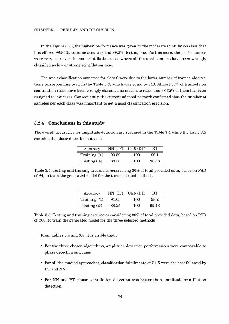
CHAPTER 3. RESULTS AND DISCUSSION
In the Figure 3.26, the highest performance was given by the moderate scintillation class that
has offered 99.84%, training accuracy and 99.2%, testing one. Furthermore, the performances
were very poor over the non scintillation cases where all the used samples have been wrongly
classified as low or strong scintillation case.
The weak classification outcomes for class 0 were due to the lower number of trained observa-
tions corresponding to it, in the Table 3.3, which was equal to 343. Almost 32% of trained non
scintillation cases have been wrongly classified as moderate cases and 68.32% of them has been
assigned to low cases. Consequently, the current adopted network confirmed that the number of
samples per each class was important to get a good classification precision.
3.2.4 Conclusions in this study
The overall accuracies for amplitude detection are resumed in the Table 3.4 while the Table 3.5
contains the phase detection outcomes.
Accuracy NN (TF) C4.5 (DT) BT
Training (%) 90.59 100 96.1Testing (%) 88.36 100 96.88
Table 3.4: Testing and training accuracies considering 80% of total provided data, based on PSDof S4, to train the generated model for the three selected methods
Accuracy NN (TF) C4.5 (DT) BT
Training (%) 91.03 100 98.2Testing (%) 88.25 100 99.13
Table 3.5: Testing and training accuracies considering 80% of total provided data, based on PSDof φ60, to train the generated model for the three selected methods
From Tables 3.4 and 3.5, it is visible that :
• For the three chosen algorithms, amplitude detection performances were comparable to
phase detection outcomes.
• For all the studied approaches, classification fulfillments of C4.5 were the best followed by
BT and NN.
• For NN and BT, phase scintillation detection was better than amplitude scintillation
detection.
74

3.2. IONOSPHERIC SCINTILLATION AUTOMATIC DETECTION BASED ON THEFREQUENCY DOMAIN FEATURES OF SCINTILLATION INDICATORS S4 AND φ60
• Strong amplitude scintillation apparition was not usually accompanied with strong phase
scintillation
Conclusion
For the automatic scintillation detection based on absolute values of S4 and φ60, all the applied
algorithms gave good performances that were highly combined to the integration of time in
the features set. Further, dedicating more cases to train the generated classification model has
improved the results.
For the automatic detection based on the frequency domain features or the PSD features, the
selected methods gave analogous results for the phase scintillation and the amplitude scintil-
lation classification, except for the BT where the phase perturbation detection was better than
the amplitude one. The same as previous part, the highest overall accuracy was given by C4.5
followed by the BT and NN, respectively.
Generally, the obtained performances depend on the set of features employed by the approach,
the consistency between training and testing data sizes was important and the balance between
the considered samples per each class was significant to improve attained results.
75


GENERAL CONCLUSION
During this master thesis, an automatic approach for detecting and identifing the iono-spheric intermittences was developed. The introduced approach consists on executingthree chosen ML algorithms over a set of collected GPS L1C/A signals by means of a
commercial ISM receiver in the Antarctica continent.
Indeed, two types of GPS L1C/A data have been addressed in the presented classificationoperation; the first dataset was characterized by its low rate (1/60 Hz) and it was based on theabsolute values of amplitude and phase scintillation indicators that are S4 and φ60, respectively.The second dataset was constituted by the PSD functions of S4 or φ60 calculated through STFTover a 3 minutes blocks and it was defined by its high rate (1 Hz).
The three executed algorithms were the C4.5, The Bagged Trees and the Neural Network.They were selected after an introductory performances analysis phase. In fact, each of them isamong the powerful ML algorithms in the classification and they have been used in previouspapers and in various domains such as the health .
More precisely, the main focus of this elaborated work aimed to compare the efficiency betweenthe Neural Network and the decision trees methods in the scintillation events classification.Knowing that, both of the C4.5 and Bagged Trees agorithms are based on decision tree generationto classify samples. Besides, the C4.5 uses a single decision tree while the Bagged Trees decisionis based on establishing ensemble of decision trees then averaging them.
The main contributions of this work were performing the scintillations classification of GPSL1C/A waves, in the Antratica continent, using both high rate and low rate data samples. Inaddition to that, presenting a multiclass classifcation approach via employing five classes in thefirst part and four classes in the second one. In this achieved study, the detection and the classifi-cation tasks were a bit different than the binary classification approaches already presented inprevious literatures. Here the developed system had to detect the event first then to classify itinto different categories.
A discussion on the attained confusion matrices was provided at the end of each studiedpart. For the automatic detection using absolute values of S4 and φ60 indices, including thetime attribute in the features set and dedicating more cases to generate the trained model wereadvantageous to improve outcomes. For the automatic detection based on the frequency domainfeatures, which were PSD of S4 and φ60, the obtained C4.5 and BT results were comparable andclose to the results reached at the end of the first part despite of the difference in the examinateddata size, rate and features.
76

3.2. IONOSPHERIC SCINTILLATION AUTOMATIC DETECTION BASED ON THEFREQUENCY DOMAIN FEATURES OF SCINTILLATION INDICATORS S4 AND φ60
However, NN achievements over the PSD features of S4 or φ60 were lower than its fulfill-ments over their absolute values features. Certainly, this reduction was due to the higher numberof considered features that led to overfitting phenomon.
In all the studied methods, the classification by means of absolute values of scintillationindicators gave an overall accuracies within the range of 95% to 100% while the classification bymeans of S4 or φ60 PSD features gave an overall accuracy between 88% and 100%. In addition tothat, always the class with the highest number of samples, in the input data, gave an accuracygreater than 96%. Therefore, providing the convenient training data size is a critical and animportant issue to enhance ML outcomes.
Finally, another contribution consists on proving and confirming that the phase and/oramplitude scintillation detection was more reliable through using the spectral contents especially,at distinguishing scintillation levels; low, moderate and strong.
77

AP
PE
ND
IX
AAPPENDIX
This thesis was based on using ML classification algorithms over GPS L1C/A data consid-
ering two features sets. The first set of features was obtained from low data rate files that
are ’.ismr’ files and it contains 13 features : S4, S4RAW, Azimuth, Elevation, φ60, φ30,
φ10, φ3, φ1, time, C/N0, SatID, Label. The second set of features was obtained from raw data
files, which are high data rate files and it contains 2050 features: label, maximum/mean of S4
(σφ) and the rest are PSD functions.
The Figure 2.5 : Diagram flow of the BT model :
It comports the next steps:
1- Reading each file of the input sets :
-In the first part: the first features set was used.
-In the second part: the second features set was deployed.
2- Cleaning the input data through deleting NaN values and filtering only GPS L1C/A data
via selecting the SVID and C/N0.
3- Forming the input matrix that was composed by N rows and M features :
In the first part : N was 13326 and M was 13.
In the second part : N was 3999 and M was 2050.
4- Splitting the input data to training and testing sets considering different sizes (80% or 50%
of total data for each stage).
5- Activating one of the validation techniques : the 5-fold cross validation or the 25% holdout
validation.
6- Selecting one algorithm among the existing ones in the classificationLearner app and
78
training the model.
7- Exporting the trained model.
8- Predicting the test target using the exported model.
9- Calculating the testing confusion matrix while the training one was generated
automatically.
10- Calculating the testing accuracy while the training one was displayed automatically.
The Figure 2.8 : Diagram flow of the C4.5 model :
It consists of the following steps:
1- Reading each file of the input sets :
- In the first part: the first features set was used.
- In the second part: the second features set was deployed.
2- Cleaning the input data through deleting NaN values and filtering only GPS L1C/A data
via selecting the SVID and C/N0.
3- Forming the input matrix that was composed by N rows and M features :
In the first part : N was 13326 and M was 13.
In the second part : N was 3999 and M was 2050.
4- Splitting the input data to training and testing sets considering different
sizes (80% or 50% of total data for each stage).
5- Generating the trained model through fitting the training data and the target than
predicting the test target using the obtained model.
6- Verifying if the generated model was overfitted or not via changing the tuning parameters
and plotting the figures.
7- Setting the values of the tuning parameters and regenerating a new model.
8- Calculating the training and the testing accuracies.
9- Calculating and plotting confusion matrix for both stages : training and testing.
The Figure 2.17 : Diagram flow of the NN(TF) model :
It consists of the following steps:
1- Reading each file of the input sets :
- In the first part: the first features set was used.
- In the second part: the second features set was deployed.
2- Cleaning the input data through deleting NaN values and filtering only GPS L1C/A data
via selecting the SVID and C/N0.
79

APPENDIX A. APPENDIX
3- Forming the input matrix that was composed by N rows and M features :
In the first part : N was 13326 and M was 13.
In the second part : N was 3999 and M was 2050.
4- Normalizing and splitting the input data to training and testing sets considering different
sizes (80% or 50% of total data for each stage).
5- Building the computations graph structure and choosing the hidden layers number,
activation functions, Output layer function and nodes number.
6- Generating the classification model: biases, weights and Gradient Descent learning
coefficient.
7- Minimizing the Gradient Descent cost function to optimize biases, weights and get its
optimum number of iterations.
8- Evaluating training and testing accuracies.
9- Calculating training and testing confusion matrices.
80


BIBLIOGRAPHY
[1] L. BREIMAN, Machine Learning, vol. 45, Kluwer Academic Publishers, 2001.
[2] J. BROWNLEE, Introduction to the python deep learning library tensorflow, (2016).
[3] C. CHENG, T. JEAN-YVES, P. QUAN, AND C. VINCENT, Detecting, estimating and correcting
multipath biases affecting gnss signals using a marginalized likelihood ratio based
method, Signal Processing, 118 (2016), pp. 221–234.
[4] F. CHOLLET, Deep Learning with Python, 2017.
[5] B. CÉSAR VANIA, M. H. SHIMABUKURO, AND J. F. G. MONICOC, Visual exploration and
analysis of ionospheric scintillation monitoring data: The ismr query tool, lsevierLtd, 104
(2017), pp. 125–134.
[6] O. F. DAIRO AND L. B. KOLAWOLE, Statistical analysis of tropospheric scintillation of
satellite communication signals using karasawa and itu-r models, IEEE 3rd Interna-
tional Conference on Electro-Technology for National Development (NIGERCON), (2017),
pp. 347–352.
[7] A. V. DIERENDONCK, J.KLOBUCHAR, AND Q.HUA, Ionospheric scintillation monitoring
using commercial single frequency c/a code receivers, Proceedings of the 6th Interna-
tional Technical Meeting of the Satellite Division of The Institute of Navigation, (1993),
pp. 1333–1342.
[8] J. J. Z. J. SANZ SUBIRANA AND M. HERNÁNDEZ-PAJARES, Tropospheric Delay, Technical
University of Catalonia, Spain, 2011.
[9] J. A. JAN VAN SICKLE, The Tropospheric Effect, dtrop, vol. 3, GEOG 862: GPS and GNSS
for Geospatial Professionals.
[10] D. JEFF AND M. RAJAT, Tensorflow: Large-scale machine learning on heterogeneous systems,
(2015).
[11] A. B. JENSON AND C. MITCHELL, Gnss and the ionosphere, GPS world, (2011).
81

BIBLIOGRAPHY
[12] Y. JIAO, J. J.HALL, AND Y. T.MORTON, Comparison of the effect of high-latitude and
equatorial ionospheric scintillation on gps signals during the maximum of solar cycle 24,
IEEE TRANSACTIONS ON AEROSPACE AND ELECTRONIC SYSTEMS, 50 (2015),
pp. 886–903.
[13] Y. JIAO, J. J.HALL, AND Y. T.MORTON, Automatic equatorial gps amplitude scintillation
detection using a machine learning algorithm, IEEE TRANSACTIONS ON AEROSPACE
AND ELECTRONIC SYSTEMS, 53 (2017), pp. 405–418.
[14] Y. JIAO, J. J.HALL, AND Y. T.MORTON, Automatic gps ionospheric amplitude and phase
scintillation detectors using a machine learning algorithm, InsideGNSS, (2017), pp. 48–
53.
[15] Y. JIAO, J. J.HALL, AND Y. T.MORTON, Performance evaluation of an automatic gps iono-
spheric phase scintillation detector using a machine-learning algorithm, Journal of The
Institute of Navigation, 64 (2017), pp. 391–402.
[16] Y. JIAO, Y. T. MORTON, S. TAYLOR, AND W. PELGRUM, Characterization of high-latitude
ionospheric scintillation of gps signals, RADIO SCIENCE, 48 (2013), pp. 698––708.
[17] G. W. H. JOSÉ ÁNGEL ÁVILA RODRÍGUEZ, MARKUS IRSIGLER AND T. PANY, Combined
galileo/gps frequency and signal performance analysis, Proceedings of the 17th Interna-
tional Technical Meeting of the Satellite Division of The Institute of Navigation (ION
GNSS), (2004), pp. 632–649.
[18] A. K.GWAL, E. MINGKHWAN, S. DUBEI, AND R. WAHI, Study of amplitude and phase
scintillation at gps frequency, Indian Journal of Radio and Space physics, 34 (2005),
pp. 402–407.
[19] P. M. KINTNER, B. M. LEDVINA, AND E. R. DE PAULA, Gps and ionospheric scintillations,
Space weather, 23 (2007), p. doi:10.1029/2006SW000260.
[20] T. S. KORTING, C4.5 algorithm and multivariate decision trees, (2014).
[21] A. R. M. WILDEMEERSCH, E. CANO PONS AND J. F. GUASCH, Impact study of unintentional
interference on gnss receivers, European Commission Joint Research Centre, 96 (2010),
p. doi:10.2788/57794.
[22] A. NAGPAL, Decision tree ensembles- bagging and boosting, (2017).
[23] S. S. NAVIGATION, PolaRxS Application Manual, 2015.
[24] A. F. NICOLA LINTY, ALESSANDRO FARASIN AND F. DOVIS, Detection of gnss iono-
spheric scintillations based on machine learning decision tree, IEEE, (2018), p. DOI
10.1109/TAES.2018.2850385.
82

BIBLIOGRAPHY
[25] C. C. NICOLA LINTY, FABIO DOVIS, Ionospheric scintillation threats to gnss in polar
regions: The demogrape case study in antarctica, IEEE, (2016), p. DOI: 10.1109/EU-
RONAV.2016.7530546.
[26] N. T. REDD, Antarctica: The southernmost continent, (2018).
[27] A. SMOLA AND S. VISHWANATHAN, Introduction to Machine Learning, Cambridge Univer-
sity Press, 2008.
83
