go for broke or play it safe? dynamic competition with
TRANSCRIPT
RAND Journal of EconomicsVol. 38, No. 3, 2007pp. 593-409
Go for broke or play it safe? Dynamiccompetition with choice of variance
Axel Anderson*
and
Luis M. B. Cabral**
We consider a differential game in which the joint choices of the two players influence the variance,but not the mean, of the one-dimensional state variable. We show that a pure strategy perfectequilibrium in stationary Markov strategies (ME) exists and has the property that patient playerschoose to play it safe when sufficiently ahead and to take risks when sufficiently behind. We alsoprovide a simple condition that implies both players choose risky strategies when neither one istoo far ahead, a situation that ensures a dominant player emerges "quickly."
1. IntroductionM Characterizing observed firm behavior in terms of R&D budgeting, Cyert and March (1963)argue that "most organizations are aware of and probably use such simple rules as per centof revenue as a guide to research and development allocations" (p. 274). In their study of themicroprocessor industry, Khanna and lansiti (1997) report that "interfirm researcher mobilityis remarkably low" (p. 406). Moreover, evidence from the microprocessor and other industriessuggests that there are frequently different paths to achieve the same goal. For example, a givenlevel of microprocessor speed can be attained through different computer architectures.
Together, the above observations suggest that, from a manager's point of view, the decisionis not just how much to spend on R&D but also how to spend it. In fact, in some cases, the maindecision may be to choose among R&D strategies with different degrees of risk. In this article, wefocus on this dimension of R&D policy. Specifically, we study the dynamics of R&D competitionwhen firms choose the variance of R&D outcomes.
We consider a differential game with two players (firms). At each moment in time, eachplayer's position is given by a real number qi. Each player's position may be interpreted asits current quality level. In the example above, qi might denote the speed of firm i's currentmicroprocessor. Player i receives a payoff flow given by 7r(qi - qj). The player's position, qi,evolves according to a Wiener process with mean g, which is exogenously given, and variance
Georgetown University; [email protected].** New York University; [email protected] are grateful to the editor, two anonymous referees, Dirk Bergemann, and various seminar audiences for usefulcomments and suggestions. The usual disclaimer applies.
Copyright U 2007, RAND. 593

594 / THE RAND JOURNAL OF ECONOMICS
ao,, which is chosen by firm i. Our goal is to characterize the pure strategy perfect equilibrium instationary Markov strategies (Markov equilibrium; ME) of this game. In other words, we wantto understand when players choose safer or riskier R&D strategies as a function of their relativeposition.
Strategic choice of risk (variance) plays an important role in sports. For example, in thefourth quarter of a (American) football game, the team that is behind calls more passing plays,whereas the team that is ahead runs the ball. Toward the end of a hockey game the team that isbehind pulls their goalie in favor of an additional offensive player, whereas the team that is aheadsubstitutes in more defensive players. In both of these situations the team that is behind is optingfor a high variance strategy, whereas the team that is ahead is opting for a low variance strategy.As the saying goes, "If you're behind you have nothing to lose."
What is common to the sports examples is that (i) we are close to the end of the game and(ii) the final payoff function is locally convex for the laggard and locally concave for the leader.For example, suppose a hockey team trails by one goal one minute from the end. In terms of finaloutcome, the payoff is the same if the team allows an additional goal, but higher if it scores anadditional goal. So, the final payoff function is convex at - 1. The fact that we are close to theend of the game makes it easy (at least conceptually) to compute the value functions. In fact, ifwe are close to the end of the game, then convexity of the final payoff implies convexity of thevalue function. Finally, by Jensen's inequality, it follows that the trailing team benefits from amean-preserving spread in the goal-scoring function.
There is no reason to suspect a priori that such reasoning should carry over to infinitehorizon games, as it seems to be the end game effect that drives the intuition.1 However, wethink an infinite horizon is a better description of real-world oligopoly competition. So, we ask,do players still adopt a high-risk strategy when behind and a low-risk strategy when ahead in aninfinite horizon game?
Consider first the case when players are very impatient. In this case, the value function isapproximately equal to the flow profit function. In general, by Jensen's inequality, risk choices aredetermined by the curvature of the value function. Thus, for very impatient players, the answerto our question is unsurprising: choice of variance is entirely dependent on the local curvature ofthe flow profit function.
Consider now the case of very patient players. Let x be the relative difference between theplayers in the game. If flow profits as a function of this state variable are bounded, and admitlimits as the state variable tends to the extremes (÷/-oo), and satisfy a single-crossing property2
at some value x*, then in Markov equilibrium, patient players choose to play it safe when aheadand to take risks when behind. Specifically, if players are patient enough, they will choose lowvariance if x > x* and high variance if x < x*. Note that we need not make any assumptionsabout the local curvature of the profit function.
The main thrust of our results is that, when players are very patient, the second derivative ofthe value function is negatively related to the current payoff level. Specifically, a lagging playerreceives a low payoff and has a convex value function; a leading player receives a high payoffand has a concave value function. Once this has been established, equilibrium strategies followfrom Jensen's inequality. So, instead of the sports intuition that a laggard has "nothing to lose,"we show that a laggard has only to gain from moving away from the current state, and does so bychoosing a high-risk strategy.
When x* > 0, both players choose risky strategies in states where x is close to zero. It followsthat, starting from a situation where players are more or less even, a dominant player will emerge
' However, some infinite horizon games may share some of the features of finite games as in the previous examples.For example, suppose that if one of the players falls sufficiently far behind, then it must exit the game, receiving a payoffof zero. See Section 4 for a related example.
I The single-crossing property we require is weaker than monotonicity.
© RAND 2007.

ANDERSON AND CABRAL / 595
"quickly." Previous research (Athey and Schmutzler, 2001; Budd, Harris, and Vickers, 1993;Cabral, 2002; Cabral and Riordan, 1994) has characterized dynamic games featuring increasingdominance, the property whereby the gap between leader and follower tends to increase inexpected value, resulting in an asymmetric outcome. In our model, players' choices do notinfluence the drift of the state variable, so that the gap between leader and follower must remainconstant in expected terms. Despite this restriction, our result shares the feature that asymmetrytends to emerge rapidly.
We compare the ME outcome with the policy that maximizes the sum of the expecteddiscounted profits of the two players (the Planner's solution). We show that the Planner willchoose either the highest or the lowest variance possible for any discount factor. This immediatelyyields that, with enough patience, the ME outcome is inefficient outside of the interval [-Ix*1,Ix*I]. However, we also show that inside this interval the equilibrium is efficient; that is,when the players are "close enough" together, the Planner's choice corresponds to the MEoutcome.
0 Related literature. Bhattacharya and Mookherjee (1986) and Klette and de Meza (1986)consider patent race models where players choose variance. Although they explicitly considertime, their models are static in the sense that firms make a once-and-for-all choice. They showthat, in equilibrium, firms choose too much risk from a social welfare point of view. The intuitionis that there is an externality in patent races: a firm's gain from anticipating its rival is less thanthe social benefit from earlier adoption.
Judd (2003) develops an explicitly dynamic patent race in continuous time. He assumes that,at each moment, each player may choose between a partial jump and a leap motion technology.Because the latter implies a bigger variation in motion (zero motion or winning the race), placingmore resources into the leap technology effectively corresponds to a higher-risk strategy. Judd'sTheorem 8 states that, if the race prize is close to zero, then social welfare would be increased ifresources were shifted from the risky R&D projects to the less risky projects.
All three papers concur that there is too much variance in equilibrium. In broad strokes, theintuition is that there is an externality in patent races: the marginal private benefit from winningthe race is lower than the social benefit as part of the increase in the probability of winning isassociated with a lower probability that others win (which would be equally good, from a welfarepoint of view); and the higher the degree of risk, the greater the probability of an immediate endto the race, and the greater the above externality. Our model, in turn, shows that the equilibriumlevel of variance may be greater, smaller, or equal to the socially optimal level. The idea is that,given the linearity of the stochastic process we consider, the social optimum is either the highestor the lowest level of variance; but if players are sufficiently apart, then the curvature of theirvalue functions must have opposite signs, and so one of them (exactly one of them) will choosethe opposite of the social optimum.
More closely related to our model, Cabral (2003) considers a discrete-time, discrete-spaceR&D game where firms choose variance. He presents a series of examples from economics andmanagement. However, his formal analysis is rather limited, as it does not include an existenceresult or a complete characterization of equilibrium strategies, both of which we provide in thisarticle.
Several authors have looked at dynamic games with the properties that (i) in each period, eachfirm is characterized by the value of its product; (ii) in each period, each firm's profit is a function ofall firms' product values; and (iii) by investing resources into R&D, a firm stochastically improvesthe future quality of its product. The list includes Budd, Harris, and Vickers (1993), Ericson andPakes (1995), Fershtman and Pakes (2000), and Hbrner (2004). One feature that is common toall of these models is that firm strategies consist of choosing the level of R&D expenditures. Ouranalysis complements theirs: we fix the level of R&D expenditures and consider the strategicchoice of risk.
© RAND 2007.

596 / THE RAND JOURNAL OF ECONOMICS
Technically, we study a (very simple) one-dimensional stochastic differential game in whichthe agents' choices affect the variance of some state variable.' The equilibrium existence theoryfor such variance choice games is not well developed. Thus, it is not surprising that existencequestions have been for the most part dodged in economic applications of stochastic differentialgames with endogenous variance. Luckily, our model is simple enough that we can apply a resultfrom Harris (1993) to establish existence. We are aware of only two other papers that proveexistence for particular variance choice games: Bergemann and V5ilimaiki (2002) and Bolton andHarris (2001). These papers consider the ME of the undiscounted game directly. Dutta (1991)establishes that in the limit, the equilibrium strategies and payoffs of the discounted game mustconverge to those of the undiscounted games when the strong long-run average payoff is used.We could also have considered the limiting equilibrium directly. Instead, we characterize theequilibrium value functions and optimal strategies, and then investigate their behavior as playersbecome infinitely patient. Given the simplicity of our model, we feel that this is the right approach.Note that in Bergemann and Vdilimdiki (2002) and Bolton and Harris (2000) the models are morecomplex, and the restriction to the undiscounted game is necessary in order to make reasonableprogress.
The article is organized as follows. In Section 3, we present the dynamic game and showthat an ME exists. In Section 4, we characterize the equilibrium in the cases when players arevery patient. We also present results for the particular case of constant sum games, and deriveimplications for industry dynamics. In Section 5, we solve the Planner's problem and investigatethe efficiency of the ME. In Section 6, we discuss some natural extensions of the basic model.Section 7 concludes the article.
3. The model and existence
N Consider the following two-player stochastic continuous time (differential) game.' At eachinstant in time, player i E { 1, 2} chooses ri E [q, 6] (q_ > 0), the variance of its motion in a one-dimensional state space. The state of the game at time t is summarized by x(t) E Rl. Conditionalon the joint choices of the two players, x evolves according to the following Ito process':
dx(t) = V/2(a1 + o2) dz(t),
where dz is the increment of a Wiener process. Let 7r(x) denote the flow profits that player 1receives, while player 2 receives profit flows 7r(-x). Let 7r have limits lim,.--, 7r(x) = Lr > -00
and lim,-,•r r(x) = 57 < co. Our proof critically depends on these limits boundedly existing. Onesituation in which this assumption would be automatically satisfied is if there is a threshold valueof i such that the laggard is eliminated from the market, so that 7r(x) would be the flow profitsfrom some outside option for x < &, and 7r(x) would be the flow monopoly profits for x > i.
We assume 7r satisfies the following single-crossing property: there exists an x* such thatI
7r(x) < (>)•(r + 5T) if and only if x < (>)x2
"Several authors have considered one-dimensional games as models of duopoly competition: see Harris and Vickers(1987), Budd, Harris, and Vickers (1993), and Athey and Schmutzler (2001). Budd, Harris, and Vickers (1993) presentsome examples of oligopoly games that satisfy the one-dimensionality restriction. Additional examples are presentedin Section 4. These examples notwithstanding, we must acknowledge that the assumption of a one-dimensional statespace is fairly restrictive, and is violated by a number of standard oligopoly models, such as logit demand with anoutside good. Referring to models of effort choice, Budd, Harris, and Vickers (1993) claim that "the effects found inthe one-dimensional model were found to be at work also in a two-dimensional model" (footnote 2). In fact, Cabral andRiordan (1994) consider a two-dimensional game and derive results similar to those of Budd, Harris, and Vickers (1993).However, it is unclear whether such extension would work in the context of variance choice.
"4 See Harris (1993) for a very thorough treatment of one-dimensional stochastic differential games.'A good (accessible) reference for basic stochastic control is Dixit and Pindyck (1994). For a more technical
reference, see Oksendal (1998).
(DRAND 2007,

ANDERSON AND CABRAL / 597
As mentioned in the introduction, this single-crossing property is satisfied by all strictly monotonicflow profit functions. However, strict monotonicity is not required to satisfy this assumption.Weakly monotonic flow payoff functions are fine as long as they are not flat around (Lr + T)/2.Finally, we assume that players discount future profits at rate r.
We will be considering pure strategy equilibria in stationary Markov strategies, which wewill henceforth abbreviate as Markovian equilibria. A Markov strategy for player i is a measurablemap a-i : (-oo, +oo) -* [a, 8].6 Given a strategy pair a = ao + ar2, the payoffs for the playersare
U, (x, ai,,o 2 ) E [fOcer ½r (x(t)) dt I x, orf0 1U2(x, or,, or2) -E [f e-r, r(-x (t)) dt I x, 0a
In summary, we have a symmetric game on a one-dimensional space, x(t) E R. The expectedmotion of x is zero, but its variance depends on the players' choices. Specifically, at each pointx of the state space, each player chooses variance within the interval [q, 6], with the systemvariance equal to the sum of the players' choices.
We now show that an equilibrium exists for this game. Fix a Markov strategy ar2 for player 2.Then player 1 's Markov best response solves:
Ut(x; 02) = sup U1(x, Orl, 02).
Assume that an optimal Markov best response aO(Oa2) exists, then Theorem 11.2.3 in Oksendal(1998) establishes that player 1 can achieve as high a payoff using aT as he can using any(measurable) strategy. That is, a Markov strategy is a best response to a Markov strategy.
The Hamilton-Jacobi-Bellman equation (HJB) associated with this maximization problemis (via Ito's Lemma):
rV,(x;0a2) = max [r(x) + (0I(x) +0 2(x)) V" (X;a 2 )]
Proposition 1. A Markov equilibrium exists, and V, = U* is continuous for i E {1, 2} in ME.
Proof We wish to apply Theorem 11.7 from Harris (1993). To do so requires we analyze a statictwo-player game in which the players choose scalars ari e [q, 15] and the payoff for player i is 7
+ri(x) - rXi
a1 + a2
where (X,, E7) R R2. Following Harris, let i-e(x, A, A,") be the set of Nash equilibrium payoffvectors for this static game, where AL = ()A, A-2) and V" = (XI', )A2). Then by Theorem 6.6 in Harris,an ME to the original dynamic game will exist if 7-e(x, X, A") is nonempty and convex for all A,A", and x.
Note that for all (A, x) such that ri(x) : rXi for all i, there is a unique equilibrium, so7Fe(x, X, A") is nonempty and trivially convex. If 7ri(x) = rXi for all i, any allowable ar is anequilibrium, and all equilibria have the same payoff vector. Finally, consider the case in whichr (x) > r. 1 and 7r 2(x) = rX2 (WLOG; this is the only remaining case to consider). In this case,
6 We focus on Markovian equilibria, rather than the more general feedback Nash equilibria for two reasons. (i)
We are specifically interested in how variance choice depends on the state variable rather than on calendar time; and(ii) by focusing on stationary Markov strategies, we dodge technical difficulties in defining time-dependent strategies incontinuous time. For a discussion of feedback Nash equilibria, see Basar and Olsder (1998). For a discussion of issuesrelated to defining time-contingent strategies in continuous time, see Simon and Stinchcombe (1989) and Bergin andMacLeod (1993).
For some intuition, substitute (k,, X7) for (Vi(x), V,"(x)) and rearrange the Bellman equation payoffs.
© RAND 2007.

598 / THE RAND JOURNAL OF ECONOMICS
the set of Nash equilibria is a, = q, 9 2 E [q, 6]. The payoff vector for player 2 is the same inevery equilibrium. The set of payoff vectors for player 1 is the convex set
[irj(x)-rXij 7rj(x)-rX1 1and thus Theorem 6.6 in Harris (1993) applies. Q.E.D.
4. Results with high patience
0 Players' attitudes toward risk will be influenced by the curvature of the flow profit function7r. If players are very impatient (high r), then the local curvature of 7r will weigh heavily in their
decision making. In fact, if r is convex (concave) in a neighborhood of x, then player 1 choosesthe risky (safe) process at x if r is above a certain threshold. Because we can provide examples offunctions that alternate between convex and concave throughout the range of x, we cannot hopefor low-patience analogs of our high-patience results. One class of examples is
(a(x) - •(ax)2
-bsinx X < 02 (X+x (1)a (a+)
2 +bsinx
with b > 2 (Figure 1).We do not find these insights for the high r case surprising or particularly interesting. Instead
we focus on what happens for low r. Given our minimal assumptions on 7r, it is not obviousa priori what the nature of the equilibrium strategy is.
[: Risk choice in the limit. Our main result is that x* divides the state space so that withenough patience, high variance is chosen by player 1 when x < x* and low variance is chosen byplayer I when x > x*. The structure of the argument that establishes this result is straightforwardand proceeds in the following three steps:
Step 1. The Bellman equation implies that sign(r V, (x) - 7r(x)) = sign( Vj'(x)). Also, the Bellmanequation is linear in variance choice with coefficient V'(x), so r V,(x) - 7r(x) > 0 implieso,(x) = 5 and r V,(x) - 7r(x) < 0 implies or,(x) = q.
Step 2. In the long run, x spends almost all of its time arbitrarily far from 0. With no drift,x is equally likely to be arbitrarily close to co and -co. Given limx.... 7r(x) = LT andlira .... r(x) = fT, we have lim,•o r VI(x) = (ir + T)/2 (Lemma 1).
Step 3. The single-crossing property combined with Step 2 implies that for any x < x*, r lowenough yields r V,(x) > 7r(x) and thus or,(x) = 5 by Step 1.
FIGURE 1
PLOT OF FUNCTION GIVEN IN (1) FOR a = 3, b = 5
X
© RAND 2007.

ANDERSON AND CABRAL / 599
First we formally establish Step 2:
Lemma 1. lim,_0 r V,(x) = (.T + Tr)/2 fori E {1, 2}.
The proof is in the Appendix.Given the results in the last section, we can conclude almost immediately that players will
pursue the safe process when ahead and the risky process when behind.
Proposition 2. For all x < x*, 3r*(x) such that orl(x) = o, Vr < r*(x). Conversely, Vx > x*,3r*(x) such that or = q, Vr < r*(x).
Proof We have 7r(x) > (i + Rf)/2 for all x > x* and 7r(x) < (L + iF)/2 for all x < x*. ByLemma 1, lim,-o r VI(x) = (r + r)/2. Finally, by the HJB equation for player 1, r VI(x) > wr(x)implies that Vl'(x) > 0, which in turn implies or,(x) = 6, while r V,(x) < 7r(x) implies thatVý'(x) < 0, which in turn implies orl(x) = q. Q.E.D.
To illustrate this results, we graphed rV,(x) (Figure 2) for differing values of r for thefollowing constant sum case:
-2 if x < -2
2+2x if -2<x <-137r(x)= !x if <X < _
2x-2 if I <x <2
2 if x>2
Because 7r = -1, f" = 2, we have 7r(O) = (Lr + jr)/2. It follows that x* = 0; that is, a patientplayer chooses low variance if and only if he is ahead by at least one unit. In fact, as Figure 2shows, even for values of r away from zero (that is, long before rV converges to a constant), thevalue function is concave below x* = 0 and concave above x* = 0, for example when r = 1/4.
Proposition 2 states that x* divides the state space, so that for all x < x* (laggard), highrisk is the equilibrium strategy given sufficient patience, whereas for x > x* (leader), low risk isbetter given sufficient patience. Figure 3 illustrates this. Notice that the figure also illustrates thatthe threshold value of r depends on the particular x considered. In this example, the closer x is tozero the lower the threshold r*(x).
Intuitively, Proposition 2 can be understood with reference to each player's HJB. Clearly, thevalue function is convex if and only if 7r(x) < r V(x). In other words, if current profit is less thanaverage discounted payoff, then "things can only get better." If things are going to get better itis because the discounted payoff in neighboring states is better than in the current state, and so ahigh-risk strategy is optimal, insofar as it will move us away from the current state. If we show that7r(x) < r V(x) for a laggard then we are done: a laggard wants to choose a high-risk strategy. So,instead of the sports intuition that a laggard has "nothing to lose," we show that a laggard has onlyto gain from moving away from the current state, and does so by choosing a high-risk strategy.
Note that in the limit, the unique equilibrium can only be one of the three types pictured inFigure 4. The knife-edged case of x* = 0 is straightforward. Note that in this case a = a + 6,which we call the medium variance case. When x* 0 0, the state space is divided into threeintervals. When x* > 0, each player chooses high variance (or = 6) around x = 0, so we callthis the high variance case. When x* < 0, we again have medium variance at the extremes, butlow variance in a neighborhood of x = 0, so we call this the low variance case. These definitionsallow us to state the following simple corollary to Proposition 2.
Corollary 1. The high, medium, and low variance cases obtain as 7r(O) is lower than, equal to, orgreater than (,y + fi)/2, respectively.
0 Example: Bertrand competition. Consider an industry with two firms in which pricecompetition takes place after R&D investments are made. Specifically, suppose that each consumer
0 RAND 2007.

600 / THE RAND JOURNAL OF ECONOMICS
FIGURE 2
HOW rV(x) CHANGES IN r
rV
2
(a) r = 10, 000
-10 -5
rV
2 A
(b) r = 25
1-
5 10x
-10 -5
x
5 10
rV,4
(c) r = 4
1
-10 -5
2
(d) r = 14
x5 10 -10 -5
I i X5 10
4-
rV
(e) r = I
-2
rV
24-
(f) r = 10,000
5 10I I
-10 -5
x
5 10
-1 -
-2
receives utility u = max{zIq 1, z 2q 2 } ± z 0, where zi is the quantity of good i, qi is the qualityof good i, and z 0 denotes other goods. Suppose that each consumer buys at most one unit fromeach firm (zi E {0, 1}) and is subject to a budget constraint such that he can only spendy. Finally,
assume that marginal cost is constant and equal across firms (with no further loss of generality,assume marginal cost is zero). Firms simultaneously set prices and consumers then choose z0, zI,z 2 . In equilibrium, consumers buy from the firm with the highest quality (say, firm i) at a pricegiven by min {qf - qj, y}. The profit function is therefore given by
0 if x <0
r(x)= x if 0O<x_<y.y if x>y
© RAND 2007.
1
Z : "'
1
I
-L
I

ANDERSON AND CABRAL / 601
FIGURE 3
THE CONCAVITY OF V(x)
ir, rV
Ir(X)
7-V(X)
X
orl =a- a
0"2 0-.-' • or0 IX*
0 --X
2-1=0-
o"2 =
("2 =-
High Variance
01 =
0-2 0
-- * 0 0
Medium Variance
o1 = 0-- 01 = 0
0"2 9 "02 = Or
X* 0
In this example, (Lr + fl)/2 = y/ 2 and thus x* = 1/2 > 0; thus, this is the high-variancecase. Corollary 1 applies: near x = 0, both firms choose high variance.
0 Example: competitive balance in sports. In sports leagues, a team's value is a function ofits competitive success as well as the overall success of its league, and the league's success is afunction of competitive balance. For simplicity, consider a league with two "important" teams.Let x be the difference in quality between the teams (e.g., the average skill of its roster). Supposethat each instant corresponds to a season and that at the beginning of the season each team getsto choose the variance of its quality change. Let p(x) be the probability of winning the leagueand v(x) the value of the league. We assume that p(x) is increasing and that v(x) is decreasing inIx 1, a measure of competitive imbalance.
Specifically, suppose that v(x) declines exponentially with competitive imbalance:
[Y + (1 -A)e-lxl if IxI < In2V(X) 0 +/A) if Ixj > ln2
where /t E (2, 1). Suppose moreover that the likelihood that team i wins each league isexponentially increasing in its quality lead: p(x)= ½ex (for values of x in [0, In 2]). Pullingall of these elements together, we have a profit function
© RAND 2007.
FIGURE 4
THE THREE ME FOR LOW r
Low Variance
01 =*
02 =-
0"1 =!Z
02 = -
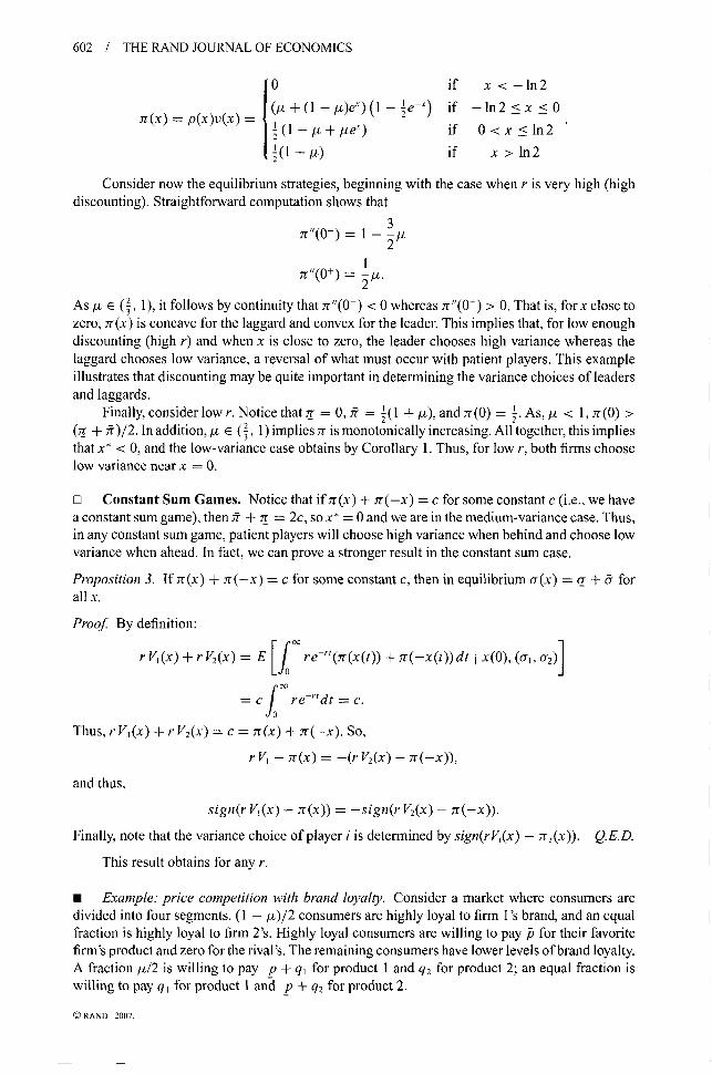
602 / THE RAND JOURNAL OF ECONOMICS
0 if x < -ln2
(it +(1I-A)ex)(1-ex) if -ln2<x<0
l (l_-/+ ie) if 0<x<ln2
+(1 A,/t) if x > ln2
Consider now the equilibrium strategies, beginning with the case when r is very high (highdiscounting). Straightforward computation shows that
37r"(0-) = 1 - 3 A
2
7r"(0+) = 2.
As /I E (2, 1), it follows by continuity that rr"(0-) < 0 whereas 7r"(0+) > 0. That is, forx close tozero, 7r(x) is concave for the laggard and convex for the leader. This implies that, for low enoughdiscounting (high r) and when x is close to zero, the leader chooses high variance whereas thelaggard chooses low variance, a reversal of what must occur with patient players. This exampleillustrates that discounting may be quite important in determining the variance choices of leadersand laggards.
Finally, consider low r. Notice that 7r = 0, 5. = !(I +/t), and 7r(0)= i.As,[f < 1, r(0) >
(Lr + f)/2. In addition, gi E (', 1) implies 7r is monotonically increasing. All together, this impliesthat x* < 0, and the low-variance case obtains by Corollary 1. Thus, for low r, both firms chooselow variance near x = 0.
El Constant Sum Games. Notice that if-r(x) + 7r(-x) = c for some constant c (i.e., we havea constant sum game), then f" + 7r = 2c, so x* = 0 and we are in the medium-variance case. Thus,in any constant sum game, patient players will choose high variance when behind and choose lowvariance when ahead. In fact, we can prove a stronger result in the constant sum case.
Proposition 3. If 7r(x) + Yr(-x) = c for some constant c, then in equilibrium a(x) = + - forall x.
Proof By definition:
r V(x) +r V2(x) = E re-r'(7r(x(t)) +.r(-x(t)) dt I x(0), (cr,, or2)
= C re-'dt = c.
Thus, r V,(x) ± r V2(x) = c = 7r(x) + 7r(-x). So,
r V, - -r(x) = -(r V2(x) - 7r (-x)),
and thus,
sign(r VI(x) - 7r(x)) = -sign(r V2(x) - 7r(-x)).
Finally, note that the variance choice of player i is determined by sign(rVi(x) - 7ri(x)). Q.E.D.
This result obtains for any r.
0 Example: price competition with brand loyalty. Consider a market where consumers aredivided into four segments. (1 - /t)/2 consumers are highly loyal to firm I's brand, and an equalfraction is highly loyal to firm 2's. Highly loyal consumers are willing to pay P for their favoritefirm's product and zero for the rival's. The remaining consumers have lower levels of brand loyalty.A fraction //2 is willing to pay p + q , for product 1 and q2 for product 2; an equal fraction iswilling to pay q, for product 1 and p + q2 for product 2.
C RAND 2007.

ANDERSON AND CABRAL / 603
Suppose that it is small and that the initial product quality levels are such that qj > P forall i. Then the unique equilibrium of the pricing game is for firms to set pi = P3, the highlyloyal consumers' willingness to pay. If jqj - qjl _< p, then mildly loyal consumers choose theirfavorite brand. If, however, qj - qj > p, then all mildly loyal consumers choose firm i instead.
This situation leads to the following profit function:
Sif X -p
7r(x)= / ½/if -_p<x < _p.
[(I + AV if p<x
This is a constant sum example, so solving for the equilibrium is straightforward. We have
r V(x) = I [J e(`sx)r7(s) ds + eýX-S)7r(s) ds]
where y = 2 r(.Ir + j) and ai = ,Ir/(l + 6), by Proposition 3. Integrating we find:
[(1 - it +/tcosh(ap)e"x) if x < - p
r V(x)= kb(l +/t sinh(ax)e•P) if - p<x< p
/(1 + A - /cosh(uP)e-"x) if p < x,
where cosh(z) = (ez + e-Z)/2 and sinh(z) = (ez - e-z)/2. We can then twice differentiate to find:
(-1211 cosh(ab)e" > 0 if x < -
r V"(x) = pa 2't sinh(ux)e-uP if - p <x <p-Da'tA cosh(ab)e-x < 0 if p < x.
Thus, firms choose the risky strategy when behind by more than P, and the safe strategy whenahead by more than jb. However, because sinh(z) is negative for z < 0 and positive for z > 0, firm1 chooses the safe strategy when x E (-,b, 0), the risky strategy when x E (0, D), regardless ofthe value ofr. Thus, x* does not behave as a cutoff as in Proposition 2.
What fails? Notice that (Lr + Tr)/2 = b/2, and that 7r(x) = b/2 for a range ofx values. Thatis, the single-crossing property is not satisfied in this example. Thus, despite the fact that rVi(x)is converging to this constant, we cannot sign rVi (x) - r (x) regardless of the value of r on thisrange.
[I How long until one player dominates? One question that has received a lot of empiricaland theoretical attention is whether R&D competition leads to increasing dominance. That is, isit the case that firms that are ahead tend to pull farther ahead, or do firms that are behind tendto catch up to the market leaders? This question concerns the expected drift in x, but as we haveruled out expected drift a priori, we cannot opine on this question as it is usually posed in theliterature.
We can, however, ask a similar question: if two firms were located close together at time 0,how long do we expect them to stay close together? Intuition suggests that the higher the variancein Ito process x(t), the faster (on average) the two firms should separate. To see this, think of theextreme case of zero variance; in that case, the two firms would never separate. This intuitionturns out to be correct. Specifically, if we let rx be the first exit time from the interval (-x, x),given x 0 E (-x, x) for some x > 0, and ExO[rx] be the expected rT given x0, then we have thefollowing proposition.
Proposition 4. Exo[rx] is highest in the low-variance case, and lowest in the high-variance case.
Proof Recall that f(x' t, x(O), a) is the probability that x(t) = x' at time t, which is a normaldensity with mean x(0) and some variance. Note that in the high-variance case the variance
© RAND 2007.

604 / THE RAND JOURNAL OF ECONOMICS
FIGURE 5
SAMPLE PATHS OF SYSTEM DYNAMICS WHEN aT = 0.5, a - 5, x* = 10
X(t)A
X*
0 >t
Ul(X) + 0 2(x) is higher for all x, thus the overall variance is higher as well. This means thatstarting from the same x(0), the probability of being outside of any interval (-x, x) at any time tis higher in the high-variance case. Thus, the expected exit time is lower. Q.E.D.
Figure 5 illustrates Proposition 4. Instead of working with a primitive 7r function, we simplyassume that x* > 0 and apply Proposition 2: if r is sufficiently small, which we assume, thenplayers choose a = ar if x > x* and ar = d if x < x*. It follows that or, + r2 = 2(7 for -x* <
x < x* and o,+ Cr 2 = q + 6 forx < - x* orx > x*. Figure 5 plots a series of equilibrium paths{x(t)} for particular values of x*, a_, d. Even though the expected motion of x is zero, startingfrom x = 0 the system moves away from the symmetry region [-x*, x*] relatively quickly.
Budd, Harris, and Vickers (1993) and Cabral and Riordan (1994) provide conditions suchthat a dynamic competitive system will move away from symmetry in expected value (increasingdominance). In both papers, the fundamental condition is the "joint profit" or "efficiency" effect:namely thatjoint profits, 7r(x) + 7r (-x), be increasing in Ix[.! Cabral (2002) shows that increasingdominance may also result when firms choose the correlation of their motion with respect to theirrivals', even if 7r(x) + 7r(-x) is constant (no efficiency effect). Our result, by contrast, requiresno particular assumption regarding 7r(x) + 7r(-x). It does not directly pertain to increasingdominance. In fact, we assume that, in expected terms, the system will remain at the currentstate x. However, Corollary 1 and Proposition 4 have a flavor similar to increasing dominance,in the sense that, if 7r(0) < (Lr + ir)/2, then the system will have a tendency to move away fromsymmetry (x = 0).
5. Equilibrium and efficiency
0 One question that has received some attention in the R&D literature is the relationshipbetween equilibrium and efficient choices of risk. Bhattacharya and Mookherjee (1986) andKlette and de Meza (1986) show that, in a static patent race model, firms choose risk levels thatare inefficiently high.' In this section, we solve for the efficient solution (i.e., the solution thatmaximizes joint payoffs), and compare this to the equilibrium solution. As we will see, the resultfrom the static patent race models does not extend to our model.
We consider an extension of the basic model as follows. Instead of two players, we nowconsider a single player-the Planner-who receives a flow payoff given by irp(x) = 7r(x) +7r(-x). The state of the game, x, evolves according to a Wiener process with zero drift andvariance ar E [2o, 26], where ar is the Planner's choice. Specifically, a Markov control for the
Cabral and Riordan (1994) consider, as we do, the limit case of very small discounting; Budd, Harris, and Vickers(1993), by contrast, consider the case of high discounting.
9 Although there is time in their models, we refer to them as static in the sense that players make a one-time decisionregarding risk level.
C RAND 2007.

ANDERSON AND CABRAL / 605
Planner is a measurable map or : (-co, +co) H-* [2a, 26]. Fix a Markov control ar and define theexpected discounted value of joint profits starting from x(0) as:
Up(x, a) - E [f e-rrp(X(t)) dt I x, a]
The social Planner then solves:
Ug(x) = sup Up(x, a)
F- Existence. Define the Hamilton-Jacobi-Bellman equation (HJB) as (via Ito's Lemma):
r Vp(x) = max [7rp(x) + a(x)Vp"(x)].
Proposition 5. A solution to the Planner's problem exists,joint profits are maximized by a Markovcontrol, and rVp(x) = r U* (x), where Vp is continuous.
Proof This is a standard stochastic control problem. Theorem 11.2.1 in Oksendal (1998)establishes the necessity of the HJB, while Theorem 11.2.2 establishes sufficiency. Finally, 11.2.3yields that the maximum is obtained by a Markov control. Q.E.D.
The Planner's solution is bang-bang if an optimal control or* can be chosen such thata* E {2o, 26CY. A Markov control or is simple if any bounded interval (a, b) C IR admits a partition{yi, i = 0,..., n}, a = Yo < y, < ... y,, = b such that o is constant on each subinterval (y, yi,,).The Planner's solution is simple if there exists an optimal Markov control that is simple.
Lemma 2. The Planner's solution is simple and bang-bang.
Proof Let a* be an optimal Markov control. Assume rVp(x) > 7rp(x). The continuity of Vp and7r then implies that there exists an E such that rVp(y) > 7rp(y) for all y E (x - e, x + E), andthus r Vp(y) < 0 and a*(y) = 2a on this interval. Like reasoning establishes that a* is equal to21 on an open interval whenever rVp(x) < 7rp(x). Finally, for anyx such that rVp(x) = .7rp(x) thePlanner is indifferent across all a, and thus we may choose an optimal Markov control & suchthat &(x) = a*(x) for all x such that rVp(x) : 7rp(x) and &(x) = 26 otherwise. Q.E.D.
o Planner's value function characterization. Now that we know that an optimal control canbe chosen such that a is constant on open intervals, we can explicitly solve for the form of thevalue function. Consider any interval on which a is constant. The HJB equation implies that:
r Vp(x) = 7rp(x) + a Vp'(x). (2)
The general solution to this differential equation is:
Vp(x) = ae" + be'x + ip(x; a),
where
Yp(x; a) I - eJ e(-x)rp(s) ds + ea(X-) 7rp(s) ds,
a and b are undetermined coefficients, y _ 21u"- > 0, a -= Irl > 0.(To verify this solution, note that it must satisfy
Vp(x) 7rp(x)+oVp'(x) _ y-2ia ar(x)± o -"[aeX+ bex+ jp(x;ca)]r y r
which is true iff y - 2aoa = 0 and U 2ra/r = 1. These two equations are satisfied for the given y
and a. Further, it must be the case that ip is bounded. To see this, take the first term in bracketsand simplify:
© RAND 2007.

606 / THE RAND JOURNAL OF ECONOMICS
J eU(s-x) P(s) ds = e` w eprep(s) ds
< e` J es2r ds
25.
where the inequality follows from the assumption that 7r is bounded (7r(s) < T").)
Direct computation yields Tr(x;o) equal to the total expected discounted value of profitsstarting in state x if or remained unchanged. Because x(t) is an Ito process, the distribution overfuture values x at time t starting from x at time t = 0 is normal with mean x and variance 2ot ifor does not change. Thus, we compute
E [j e-"'rp(x(t)) dt x(0) = x, a]
= J0 e-7rp(s)(47rat)-Je--(4, dtds
= fe [f4at e - -dt 7rp(s)ds + (47ro-at'e`-e- •t dt f rp(s)ds.
Evaluating the bracketed expressions yields the desired result.For an intuition of why this must be so, note that the value function is bounded and must
always satisfy the general form of Vp. If the Planner chooses or(x) equal to a constant, the valuefunction has the same form for all values of x, yet Vp(x) is unbounded unless a = 0 and b = 0.Thus, if no one switched projects, Vp(x) = ip(x; a).
As i'p is the value when no one switches projects, then the other two terms must be the valueto the Planner of the option to switch projects, which implies a, b > 0.
E The patient Planner case. We know that the Planner will either choose the highest or lowestpossible variance, as the solution is bang-bang. It turns out that there is a simple condition thatdetermines which extreme the Planner will choose near x = 0 as long as the Planner is patient.As in ME, the Planner's choice will be determined by the local curvature of the profit functionfor high enough r. Thus, we focus on what happens for low r. Substituting 7rp for 7r in the proof
of Lemma I yields a similar result for the Planner's value.
Lemma 3. lim,_0 r Vp(x) = j + Tr.
[] Efficient variance choice when firms are "close". Given the results in the last section, wecan offer a simple condition that determines the Planner's choice of variance near x = 0 givenenough patience.
Proposition 6. If x* > 0, then Vx E (-x*, x*), 3r* > 0 such that the Planner sets a(x) = 25
for all r < r*. Conversely, if x* < 0, then Vx E (-lx*1, Ix*1), 3r* > 0 such that the Planner setsa(x) = 2or for all r < r*.
Proof If x* > 0, then 7r(x) < (g + Tr)/2 for all x < x*, while 7r(-x) < (L + T")/2 for all x >-x* so that Vx E (-x*, x*), 7rp(x) =_ 7r(x) + 7r(-x) < 7" + ff = limr-o r Vp(x) (by Lemma 3).Finally, by the HJB equation for the Planner, 7rp(x) <rVp(x) =• Vp(x)> 0 =ý a(x)=
2E. Q.E.D.
We are able to characterize the patient Planner's variance choice on the interval (-Ix*I, Jx*I)
but not outside of this interval. To do so, we would need to assume that 7rp satisfies the single-
crossing property. Notice that none of the examples we have presented satisfy this property.
( RAND 2007.

ANDERSON AND CABRAL / 607
w Equilibrium and efficiency. We are now ready to compare the equilibrium outcome withthe Planner's solution. Notice that the Planner will always choose the highest or lowest variancepossible. Thus, whenever the players choose different variances in ME, the ME is inefficient. ByProposition 2, the players choose different variances outside of the interval (- x*I, jx* ) forr lowenough, whereas by Propositions 2 and 6, the Planner's choice corresponds to the ME on thisinterval. Thus we have:
Corollary 2. For r low enough, total variance in ME is socially efficient in [-Ix*l, Ix*j] andinefficient outside of this interval.
6. Extensions
0 There are a number of ways in which the simple model presented here could be extended.In this section we will consider three of them: making the variance term a more general functionof player choices; adding exogenous drift; and adding in cost of variance to the flow payoffs.
Instead of the linear specification considered here, we could instead have the instantaneousvariance be some more general function E(9 1 , 0r2). As long as E is bounded away from 0 and 00and monotonic in both oI and r2 individually, all of our results extend trivially. Thus, our resultsare not driven by our linear specification.
We assumed no drift in x(t). The first step to relaxing this assumption would be to assumesome exogenous drift, A(x). Our existence results extend immediately with this change. The lowr characterization results are a bit more delicate. With drift, the Bellman equation becomes
r VI(x) = max[7(x) + A(x)V,'(x) + (Cr(x) + 0r2(x))V,"(x)].•,l (x)
There are two issues: first, the limit of V'I(x) must be characterized. Intuitively, this should tendto 0 as r tends to 0, but the proof is not as straightforward as the proof for rV,(x).
If V'1(x) tends to 0, then our result would extend as long as 7r < lim,_•0rV,(x) < fr.Examining the proof of Lemma 1, the key is what happens to the mean of x(t) relative tothe standard deviation as t --+ o. More specifically, x(t) will be distributed normally with meanm(t, x(O), it) and standard deviation s(t, x(O), a). To retain 7r < lim,_ 0 r Vi(x) < fr, we need
lim m(t, x(0), I)/s(t, x(0), a)
bounded. Thus, we need m(t, x(O), At) and s(t, x(O), a) to grow at the same rate. In our model,s(t, x(O), a) is of the order IT. If we simply assumed that A(x) = /t (i.e., a constant), we wouldhave m(gt, t) = At and lim,- m(Az, t)/s(t, x(0), a) = oo. One natural way to deal with this issuewould be to make the process mean-reverting.
Another extension would be to include a cost function for different variance choices:c(ar). What shape should such a cost function be? In most applications, the cost of settingeither very low variance or very high variance is likely prohibitive. Thus, one might consider aU-shaped cost function. One immediate technical difficulty is existence of a pure strategy ME.Our straightforward proof fails with the addition of cost of variance, but can be rescued byallowing mixing. Specifically, modify the Bellman equation by making flow payoffs 7(x) -c(ora(x)), which implies a first-order condition Vj"(x) = c'(ao(x)), and a satisfied second-ordercondition -c"(aj(x)) < 0. Thus, from the first-order condition and the U-shaped cost function,ao(x) will be monotonically increasing in Vj'(x). Again, rVi(x) will tend toward the average ofthe flow payoffs at the extremes. Intuitively, rI (x) will be increasing in x.
7. Conclusion
N Conventional wisdom from sports indicates that, close to the end of a game or race, thelaggard should choose a high-variance strategy and the leader a low-variance strategy. In fact, thelaggard has "nothing to lose": his payoff does not decrease if he falls farther behind but his valuemay increase substantially if he moves ahead; in other words, his value function is convex. In
© RAND 2007

608 / THE RAND JOURNAL OF ECONOMICS
this article, we consider the situation of an infinite race. We show that, if players are sufficientlypatient, then a laggard, if sufficiently behind, will choose a high-variance strategy, and the leadera low-variance strategy.
The summary intuition for our result is derived from the HJB equation, which in our gamebecomes
r V(x) = 7r(x) + (or, + o 2) V"(x).
This implies that the second derivative of the value function is negatively related to the currentpayoff level. Specifically, a lagging player receives a low payoff and has a convex value function,whereas a leading player receives a high payoff and has a concave value function. Finally, Jensen'sinequality implies that a lagging player chooses high variance, whereas a leading player chooseslow variance.
We also show that, with enough patience, the ME outcome is efficient when players are closeenough together and inefficient when players are sufficiently far apart.
Appendix
El Proof ofLemma 1.
Proof We shall establish the result for rVj; the proof is nearly identical for rV2. Let f(x' It, x(O), u) be the probabilitythat x(t) = x' at time t, given starting value x(0) and Markov control a. As x(t) is an Ito process, f is a normal densitywith mean x(O) and some standard deviation s(t, x(O), o), where lim,-_ s(t, x(0), a) = oc. To simplify notation, let
g(t I x(0), 'a) = a(x')f(x' It, x(0), c) dx'.
Claim 1. lim,- g(t I x(O), a) = (LT + fr)/2.
ProofofClaim 1. Fix any 5 > 0, then:
11 2 2
f(x' It,x (0), o) dx'= + 7 ,o e- dz.
So, lim,_ f(x' I t, x(O), a) dx'
- + lim I e- 2dz
2'
where the last line follows from the fact that lim,_o s(t I x(O), ar) -o.
Similar steps establish that:
f-1lim f(x'It, x(O),a)dx' 2 X > 0.
Thus,
limn Jf(x'lt,x(0),a)dx' 0 Vx> 0,
and so,
lim f 7r(x')f(x'It, x(O), c)dx' = 0 V.i > 0.
Together these imply that
lim g(t I x(0), a) = lim 7r(x) + - lim 7r(x) = (Lr + ff)/2,I 2 xcc 2
and we have established Claim 1.Now for any optimal Markov control a, we have:
r V,(x) f re-,g(t I x(O), o)dt.
© RAND 2007.

ANDERSON AND CABRAL / 609
Integration by parts yields:
r VI(x) = [-e`"g(t Ix(O),o')]'o + e`"g,Q Ix(0), u)dt
- 0 +g(O I x(O), a) + e- "g,(t I x(O), a)dt.
So that,
lim r VI (x) = g(0 I x(O), ) +lim e-"g,(t I x(O), a) dt
= g(O I x(0), a) + lim g(t Ix(0), a) - g(O Ix(0), o-)
= lira g(t I x(0), a),
which by Claim I equals (Zr + u)/2. Q.E.D.
References
ATHEY, S. AND SCHMUTZLER, A. "Investment and Market Dominance." RANDJournal of Economics, Vol. 32 (2001), pp.
1-26.BASAR, T. AND OLSDER, G.J. Dynamic Noncooperative Game Theory. Philadelphia: Society for Industrial and Applied
Mathematics, 1998.
BERGEMANN, D. AND VALIMAKI, J. "Entry and Vertical Differentiation." Journal of Economic Theory, Vol. 106 (2002),pp. 91-125.
BERGIN, J. AND MACLEOD, B. "Continuous Time Repeated Games." International Economic Review, Vol. 34 (1993), pp.21-37.
BHATTACHARYA, S. AND MOOKHERJEE, D. "Portfolio Choice in Research and Development." RAND Journal of Economics,Vol. 17 (1986), pp. 594-605.
BOLTON, P. AND HARRIS, C. "Strategic Experimentation: The Undiscounted Case." In P. Hammond and G. Myles, eds.,Incentives Organization and Public Economics: Essays in Honour of James Mirrlees. Oxford: Oxford UniversityPress, 2000.
BUDD, C., HARRIS, C., AND VICKERS, J. "A Model of the Evolution of Duopoly: Does the Asymmetry between Firms Tendto Increase or Decrease?" Review of Economic Studies, Vol. 60 (1993), pp. 543-573.
CABRAL, L.M.B. "Increasing Dominance with No Efficiency Effect." Journal of Economic Theory, Vol. 102 (2002),pp. 471-479.
"R&D Competition When Firms Choose Variance." Journal of Economics and Management Strategy, Vol. 12(2003), pp. 139-150.
-- AND RIORDAN, M.H. "The Learning Curve, Market Dominance and Predatory Pricing." Econometrica, Vol. 62(1994), pp. 1115-1140.
CYERT, R.M. AND MARCH, J.G. A Behavioral Theory of the Firm. Englewood, NJ: Prentice-Hall, 1963.DixIT, A. AND PINDYCK, R. Investment under Uncertainty. Princeton, NJ: Princeton University Press, 1994.DUTTA, P. "What Do Discounted Optima Converge To?" Journal of Economic Theory, Vol 55 (1991), pp. 64-94.ERICSON, R. AND PAKES, A. "Markov-Perfect Industry Dynamics: A Framework for Empirical Work." Review of Economic
Studies, Vol. 62 (1995), pp. 53-82.FERSHTMAN, C. AND PAKES, A. "A Dynamic Oligopoly with Collusion and Price Wars." RAND Journal of Economics,
Vol. 31 (2000), pp. 207-236.HARRIS, C. "Generalized Solutions of Stochastic Differential Games in One Dimension." Working Paper, Nuffield College,
1993.-- AND VICKERS, J. "Racing with Uncertainty." Review of Economic Studies, Vol. 54 (1987), pp. 1-21.
HORNIR, J. "A Perpetual Race to Stay Ahead." Review of Economic Studies, Vol. 71 (2004), pp. 1065-1088.JUDD, K.L. "Closed-Loop Equilibrium in a Multi-Stage Innovation Race." Economic Theory, Vol. 21 (2003), pp. 673-695.KHANNA, T. AND IANSITI, M. "Firm Asymmetries and Sequential R&D: Theory and Evidence from the Mainframe
Computer Industry." Management Science, Vol. 43 (1997), pp. 405-421.KLETTE, T.J. AND DE MEZA, D. "Is the Market Biased against Risky R&D?" RAND Journal ofEconomics, Vol. 17 (1986),
pp. 133-139.OKSENDAL, B. Stochastic Differential Equations. Berlin: Springer-Verlag, 1998.SIMON, L. AND STINCHCOMBE, M. "Extensive Form Games in Continuous Time: Pure Strategies." Econometrica, Vol. 57
(1989), pp. 1171-1214.
© RAND 2007.

COPYRIGHT INFORMATION
TITLE: Go for broke or play it safe? Dynamic competition withchoice of variance
SOURCE: Rand J Econ 38 no3 Aut 2007
The magazine publisher is the copyright holder of this article and itis reproduced with permission. Further reproduction of this article inviolation of the copyright is prohibited. To contact the publisher:http://www.rand.org