' ~ ~ Computer Graphics, Volume 23, Number 3, July 1989

Goal-Directed, Dynamic Animation of Human Walking

Armin Bruderlin Thomas W. Calvert

School of Computing Science Simon Fraser University

Burnaby, British Columbia, Canada V5A 1S6

ABSTRACT

This paper presents a hybrid approach to the animation of human locomotion which combines goal-directed and dynamic motion control. Knowledge about a locomotion cycle is incorporated into a hierarchical control process. The desired locomotion is conveniently specified at the top level as a task (e.g. walk at speed v ), which is then decomposed by application of the concepts of step symmetry and state-phase-timings. As a result of this decomposition, the forces and torques that drive the dynamic model of the legs are determined by numerical approximation techniques. Rather than relying on a general dynamic model, the equations of motion of the legs are tailored to locomotion and analytically constrained to allow for only a specific range of movements. The dynamics of the legs produce a generic, natural locomotion pattern which is visually upgraded by some kinematic "cosmetics" derived from such principles as virtual leg and determinants of gait. A system has been implemented based on these principles and has shown that when a few parameters, such as velocity, step length and step frequency are specified, a wide variety of human walks can be generated in almost real-time.

CR Categories and Subject Descriptors: 1.3.7: [Computer Graphics]: Three-Dimensional Graphics and Realism Animation; G.1.7: [Numerical Analysis]: Ordinary Differential Equations. Keywords: Animation, goal-directed animation, human figure animation, dynamics, kinematics, inverse kinematics.

1. INTRODUC'I'ION

The specification and control of motion in human figure animation has always been a challenge, but two recent trends promise to relieve the tedious work of the animator. One involves high-level, goal-directed control, which reduces the amount of detail necessary to define a motion; the second involves applying dynamic analysis to the motion control process, leading to more realism in movements.

In traditional keyframing [13], the quality of a motion is usually directly proportional to the number of key positions specified. If the desired movements are complicated, the animator, rather than the system, does motion control. It has been recognized that if the

Permission to copy without fee all or part of this material is granted provided that the copies are not made or distributed for direct commercial advantage, the ACM copyright notice and the title of the publication and its date appear, and notice is given that copying is by permission of the Association for Computing Machinery. To copy otherwise, or to republish, requires a fee and/or specific permission.

excessive amount of specification for character animation is to be reduced, higher level motion control is necessary [2, 7, 17]. At the lowest level, all movements are expressed by joint rotations over time, but these joint rotations must be coordinated within a limb, between limbs and are subject to the interaction of the whole figure with its environment. By incorporating knowledge or rules about these inter-relationships, tasks like grasping or jumping can be automated and presented to the user as pararneterized goals. In such a goal-directed system, the global coordination of a motion is done by the computer. However, movements are still executed kinematic :fly at the lowest level, and the impact of physical laws such as gravity or collisions on the motion process are ignored. To achieve realistic and natural movements, dynamic analysis must be applied as a motion control technique. By simulating the real world, objects move as they should move, according to physical laws. The drawback is that the animator has to specify motion in terms of forces and torques; this is neither intuitive nor easy, and it is complicated by the computationalty expensive character of this approach. In the past, simulation of human figures concentrated on simple, elementary movements not involving coordination between several limbs (e.g. raising an arm or dropping an arm under the influence of gravity). By combining a goal-directed higher level control with dynamic simulation of motion, a system can be developed for economic and realistic animation of many co-ordinated human movements.

This paper introduces such a method for the purpose of animating human locomotion. To this end, we have implemented the KLAW (Keyframe-Less Animation of Walking) system to animate walking. Dynamic simulation provides the low-level control; a dynamic walking model, inspired by research in robotics [12] and biomechanics [4] produces a generic walking pattern from different sets of analytically constrained equations of motion which are applied as appropriate to the current state of the locomotion. Kinematic algorithms are applied to calculate all the body angles from the motion of the dynamic model. The dynamics, in turn, are regulated by a higher level control; the proper forces and torques which generate a desired locomotion are calculated as a result of a stepwise decomposition of a few walking parameters specified by the user. Thus, motion is specified conveniently and realistic animations are obtained based on the dynamic equations of motion without explicit specification of forces and torques.

The goal-oriented approach used in this paper builds on the work of Zeltzer [16], who developed a task-oriented system to animate human locomotion; although tasks like walking and jumping were implemented, the calculation of the joint angles were done kinematically and based on interpolation methods and clinical data. Thus it was not possible to easily realize variations in locomotion by changing step length or speed. The general

©1989 ACM-0-89791-312-4/89/007/0233 $00.75

233

'89, Boston, 31 July-4 August, 1989

approach to dynamic analysis which we have adopted is based on the work of Wilhelrns [15], Armstrong [1] and others [3, 11]. Perhaps the most comprehensive approach is that of Wilhelms, who produced Virya, a dynamic system for the animation of human figures which also allows for kinematic and hybrid kinematic-dynamic motion specification. In the dynamic mode, however, forces and torques have to be input in order to achieve a motion. Badler et al. [2] have been developing kinematic techniques to animate human figures. They have proposed a higher level of control, where goals such as reaching for a certain position can be defined and the joint angles are found using inverse kinematic algorithms. They also investigated dynamic and kinematic animation of specific tasks (e.g. movement in a space vehicle). A system to animate legged figures was developed by Girard and Maciejewski [8]; dynamic control was applied to the body as a whole, and the legs were specified kinematically. The problem of constraining a foot to be on the ground during its support phase was formulated as an inverse kinematics problem and solved by means of a pseudoinverse jacobian.

2. THE KLAW SYSTEM

2.1 Overview Legged locomotion describes an intricate activity where body

translation results from rotational movements in the lower limbs; problems such as coordination between the legs, proper timing of the individual leg motions and balancing of the upper body have to be addressed. It is clear that humans and other animals, however, are able to walk effortlessly without conscious thought. This is because they are inherently goal-directed [17]. Rather than thinking in terms of forces and torques, humans walk with certain goals like speed or step length in mind - - thus, a hierarchical control scheme is well suited to animate human locomotion. Figure 1 gives a structural outline of the KLAW system. The animator specifies a desired walk with up to 3 fundamental locomotion parameters which largely determine the pattern of motion and gait: forward velocity (v), step length (sl) and step frequency (sf). A major concern in constructing a goal-directed system has been the degree to which a task should be parameterized. The animator should have access to a simple, yet flexible set of movement commands that can generate a variety of instances of a task. In KLAW, therefore, in addition to the 3 locomotion parameters, up to 28 locomotion attributes [5] may also be specified which individualize the locomotion. The default values of these attributes may be modified by the animator. Examples are: lateral distance between the feet, toe clearance during swing, and maximum rotation and llst of the pelvis. After parameter specification, the system computes and outputs the body angles as functions of time - - these drive the animation of a human figure.

2.2 Levels of Control Knowledge about a locomotion cycle occurs at three levels: the

conceptual abstraction (high-level), the gait refinements (middle- level) and the physical abstraction (low-level). The conceptual level contains a few gait-specific rules or laws. These are utilized to transform the locomotion parameters into step constraints which are fed to the low-level control to "guide" the dynamic simulation of the legs. The middle-level control is responsible for the coordination of the motion and functionally operates much like a finite state machine as suggested by Zeltzer [16]. For instance, upon a "heel-strike" event, the state "single support" is changed to "double support". Hierarchically, the middle-level control manifests a stepwise reduction in the number of degrees of freedom along with a decrease in the levels of coordination (e.g. the single support state of a walk consists of a stance and a swing

234

Locomotion p ~ h i g h - l e v e l control arameters ~ . . . . . . . . . .

I / ............. ! . . . . . . : Conceptual / m Symmetry of Step~ 1 Abstraction ~ 1

, EState-Phase Timings.~ ! middle-level control

Cons~ 'a i n r s ~'States BLJUUUIO OU~JOOIt,~ [:~OIII910 OUppOlt~ I

. . . . . . . . . . . . . . . . . . .

• NApproximation E ~ o f ~ a g r a n g e ~ L o ~ o m ~ t t ~ ] I~ Forces, Torquos~--l~ M0ti0 n ~" r - - - - - -~Modo l s~

,' I I COflgrO feedback r . . . . . . . . . . . . . . . I

Abstraction .,, J L t LowerBody Lower uooy M . . . . . . . . . . . . . . . . . . . . . . . . ;

.~.og/es Kinematics ~"a it Determinants| =~ J ,, . . . . . . . . . . . . J_ , :

t l . . . . . . . . . . . . . . . . . . . . . . . . . . Pelvic Movement Compensation Upper Body ~, Kinematics ............ "~"

. . . . . . . . . . . : : : : : : : : : : : : : : : : : : : : : : . . . . . . .

Body Angles

Figure 1: Schematic diagram of the control hierarchy in KLAW.

phase). The bottom level is represented by sets of specialized equations of motion; in fact, the phases are divided into subphases in which the equations are further constrained analytically. The low-level control uses the step constraints (which essentially are the durations and final leg angles for the stance and swing phases of a locomotion step) as conditions for a special kind of a boundary value problem. That is, the equations of motion are solved by approximating the forces and torques until the constraints are satisfied. For example, the simulation of the swing leg for the current step is repeated by varying the joint-torques until it swings forward in the exact time required and heel-strike occurs with the desired hip and knee angles. In practice, this process converges quite quickly.

2.3 Dynamic Model A principal objective is to keep the dynamics simple, otherwise

the internal calculation of the forces and torques becomes infeasible. As shown in figure 2, the swing leg is represented by two segments. The stance leg supports the upper body and is implemented as a length-changing telescopic segment which simulates knee flexion in the early part and plantar flexion of the ankle in the latter part of the stance phase (as explained later, for animation, a full leg with knee, ankle and metatarsal joints are superimposed). This approach is chosen since a linear force along the leg axis is much easier to control than additional torques at the leg joints.

The segment masses are assumed to be constant and the segments to be symmetrical. The latter implies that the principal axes of inertia are identical to the anatomical axes of rotation, and therefore the products of inertia are zero. Thus, the distribution of mass is solely defined by the moments of inertia which are calculated as described in appendix B. This simplification is justified for dynamic analysis in computer animation, since it has

~ Computer Graphics, Volume 23, Number 3, July 1989

i°¢ (xh,Yh

/ /(x,y)/ /

a) stance leg model with upper body b) swing leg model (inverted double pendulum with telescopic leg) (double pendulum)

Figure 2: Dynamic models for the different phases in locomotion. 03 is negative in this configuration, all other angles are positive; see appendix B for anthropometric values.

no significant effect on the motion. The equations of motion are derived by the method of Lagrange [14] as shown in appendix A.1 and A.2. The ground constraint for the stance phase is implemented as an analytical constraint; assuming that the "dynamic foot" does not move during stance, the two degrees of freedom, x,y, are removed. In this way, there are a total of only 5 degrees of freedom (w, 01 , 0 z , 03, 04) and consequently 5 second order, nonlinear equations of motion. The equations are solved by an A-stable, standard numerical integration method [9] which has produced numerically stable results for this problem.

2.4 Control Principles The execution of the different components in KLAW is based

on four assumptions or principles: 1. The control hierarchy as illustrated in figure 1 is applied to each step of a walking sequence where a step is defined as the double plus the single support state (see also figure 3). While the high- level concepts are executed before the impending step, the low- level motion control takes place during the step. Thus, KLAW is able to adapt to changes in the locomotion parameters from step to step, i.e. accelerations and decelerations in the motion are possible with a granularity of one step. 2. Lower body dynamics and kinematics must be executed simultaneously. The dynamic simulation produces the generic locomotion pattern which is visually upgraded by kinematic measures. As explained in section 4, a human leg is superimposed onto the telescopic stance leg according to the virtual leg principle, and gait determinants like pelvic rotation or list get injected into the one-hip dynamic model. In a sense, the equations of motion guide the lower body kinematics, but the kinematic computations may, in turn, affect the dynamics. For instance, the simulation of the swing leg, where the foot is assumed to be locked, has to take into account the updated position of the heel as a result of the kinematic foot rotation, in order to achieve heel- strike properly at the end of a step. Similarly, the kinematic pelvic rotation can actually lower the hip during the swing phase, which might "force" the dynamic leg to increase its hip torque to avoid stubbing its toe. Though considerable kinematic "cosmetics" are applied, the dynamics are the very heart of the control for they guarantee natural looking rotational movements of the legs.

3. It is assumed that the upper body follows or depends on the lower body movements. Whereas the dynamic model accounts only for a natural forward and backward motion of the upper body (02 ), the angles of the arms as well as the rotations in the shoulder and spine which compensate for pelvic movemehts are expressed as functions of the corresponding angles in the lower body. The arms, for example, swing forward with the opposite legs. Thus, these angles are calculated after the dynamic simulation. 4. The last assumption concerns the dynamic model discussed above: the simulations for the stance and swing phases are separated which greatly simplifies the control as well as the numerical integration process. The rationale is that the stance leg model constitutes the major propulsive element in bipedal locomotion. It supports the body and influences the swing leg by its hip motion. On the other hand, the swing leg has little or no effect on the stance leg and the upper body. Of course, this is not completely true in real human walking, but it can be justified by the fact that the mass of the leg is small compared to the total mass of t h e body (approx. 16 %). Hence, the swing leg does not change the inertia of the body significantly unless the motion during swing happens veery suddenly, which is hardly the case for a moderate walk. Therefore, for each step, the simulation of the stance phase is executed first followed by the swing phase dynamics which incorporate the position of the hip (x h, Yh ) from the stance phase.

3. HIGH-LEVEL C O N C E P T S This section gives a discussion of the high-level control module

whose task is to transform the 3 locomotion parameters v, sl and sf into the step constraints for the low-leveI control. At least one locomotion parameter (e.g. desired velocity) has to be input by the animator. If all 3 of the parameters are not specified, the system completes the parameters using a normalization formula (the parameters are also checked at this point to ensure that they are within anatomical limits defined by locomotion attributes, e.g. sfmax= 182steps~rain). Once the locomotion parameters are accepted and specified, the step frequency and the state-phase-timings are applied to determine the durations of the stance and swing phases, and the step length is used with the symmetry of steps concept to compute the final conditions for each phase of the current step.

sta tes

phase

HSL "FOR HSR TOL HSL

single single support (right)

:E

support (left)

loft s t ance

right sw ing =

0 % 1 s top 5 0 %

loft swing ~ A v ~

right stance

HSL = heel s t r i ke left HSR = hee l s t r i ke right = l e e o l l r ight TOL = toe off le~l

Figure 3: Locomotion cycle for bipedal walking.

1 0 0 %

Since rhythmic locomotion is just a series of recmTing movements with the natural period of one stride (the locomotion

235

'89, Boston, 31 July-4 August, 1989

cycle), it is sufficient to compute movements for one cycle. The human walking cycle has been thoroughly s t u d i e d - see Inman [10], for example. For bipedal walking, a locomotion cycle

consists of two steps. As long as a symmetric gait is assumed where the left and right leg perform the same movements, just shifted in time, the principal unit of locomotion can be reduced to one step (see figure 3). Walking is possible at a wide variety of combinations of sl and ST ( v = s l . s f ) . However, a person, when asked to walk at a particular velocity, is most likely to choose parameters which minimize energy expenditure. This observation is expressed in the experimentally derived equations [10], called normal iz ing fo rmu lae , which show a linear relationship between sl and ST, where sl and body_height are measured in m, and s f in s teps / ra in :

sl = 0.004 (1)

s f . body_height 1J V

¢=> s f 2 = 0 . 0 0 4 . b o d y _ h e i g h t ' because of sl = -~ .

T h e body_height normalizes the equation. It indirectly represents the length of the legs, which has an effect on the preferred step length. Based on equation (1), the locomotion parameters are now checked and supplemented if at least one is specified. For instance, if a velocity is defined, a "natural" step length and step frequency are calculated; in the case where a velocity and a step length are specified a more angular motion might result if the step length deviates significantly from the "natural" one (see also figure 10).

The step frequency is the input to the s ta te-phase- t imings calculation. A walking cycle consists of two steps (figure 3), each step having one double support state ( d s ) where both feet are on the ground and one single support state where one foot is off the ground. With respect to timing of the individual legs the following holds, assuming t to denote a duration:

tstep = tstance--tea and tstep = tswing+tdx. (2)

Experimental data [10] suggest that in human walking there is an approximately linear relationship between the step frequency and the duration of the double support state as a percentage of a cycle, i.e. the duration of the double support state decreases with increasing step frequency. As tea vanishes, walking becomes running. Based on results from different experiments, tds can be

described in terms of s f and tcycl e :

tea = ( - O. 16 . s f + 29.08 ) . tcyde / 100 .

length, the angles of the legs measured from the vertical are identical. That is 0 t = 03 at times t ] , t 2 and t 3 . Further, 0] and 03 depend only on the step length s l . Most importantly, this remains true when the body is accelerating or decelerating, indicated in figure 4 by the increased step length at time t 3 (i.e. the body accelerated from t 2 to t 3 ).

t 1 12 13

V ' 'V

sl , ~ LL = left leg RL = right leg

Figure 4: Symmetry of compass gait for different step lengths.

This principle is now adapted to the model in figure 5 to determine w, 01 and 03 at the end of a step (heel strike) utilizing the current step length s l , Although the actual step configuration at heel strike is no longer symmetric because of the introduction of a kinematic foot for the swing leg, the basic idea can still be applied. We just imagine the symmetric step situation when the foot is flat on the ground some time after impact (illustrated by the dashed line) and calculate "back in time". For this purpose, the step length sl is measured between ank/e 1 and ankle 2 . The effect of the foot at heel strike is that the absolute value of 03 is smaller

than it would be without a foot (also, 03 < 01 ). In addition, the foot raises the position of the hip at impact, which has to be compensated by lengthening the telescopic stance leg beyond its initial length, i.e. w > l 1 . The origin for the simulation of the stance leg stays fixed at ank/e 1 , which is at a distance l 9 above the ground.

For the following calculations, it is assumed that the ground is at zero height and 05 at impact is specified as one of the

locomot ion attributes. Given l l , 1 s , 19 ' 111 and cos ( co 8 ) = t1~/8, the

application of the cosine law yields

Since s f is known as one of the locomotion parameters, and because of

2 tcycl e = 2" tstep -

sT'

t~ can be determined, and consequently the values for tstance and Iswing are obtained from equation (2). It should be noted that the length of the stance phase is greater than a step, i.e. tstance = tst" + tea (see figure 3). To simplify implementation and to satisfy t~e step-oriented control principle (assumption 1.), the stance phase of a leg is only simulated for the duration of a step and at heel strike, when the stance phase of the leading leg starts, the continuing stance phase of the hind leg is completed kinematically.

Step symmet ry is based on a compass gait (figure 4), and means simply that at heel strike, provided that both legs are of the same

r 2 =

(03 =

Since

ankle 1 =

112+171 - 2 l 1 111 COS ( 0 5 + 00 8 ) ,

c°s'S T~77 '

( x a, ya ) = (xnh, + l 8 , l 9)

heel

hip =

it follows that

and

where x~ , is xnh from previous step, and

= ( x ~ , y , ~ ) = ( x + s l - l s , O )

(xh , Yh) = (Xa+S_ l 4"1. 2 _ 2" ( x ~, - x h ) 2 ) ,

236

~ Computer Graphics, Volume 23, Number 3, July 1989 . . m i r t H . i r a , , i l l

stance le 9 /

/ jj~'

anklet & sl/2 ~- I

!

/ / / / Y / 1 / I I I I I I I I J I

!

w ~p ing leg

r ~ , ~

0 5 - ~ - ~ 1 ankle 2

]5 l

I l i l / 1111 hee, I 111 sl i

k !

Figure 5: Dynamic model at heel strike: the swing leg is extended, a foot has been added kinematically, the upper body is ignored;

0 3 is assumed to be negative, all other angles are positive.

w = ~ ( y h - y a ) 2 + ( ; ) 2

01 = sin "1 ~

0 3 = - c o 3 - sin "1 . (3)

These are the 3 final conditions for a locomotion step; together with the durations for the leg phases they form the step constraints that govern the execution of the low-level control and determine the motion by leading to the internal calculation of the applied forces and torques.

4. LOW-LEVEL CONTROL The low-level control generates the actual motions by

application of a mixture of dynamic and kinematic algorithms. The essence of this control is explained in this section and a full discussion can be found elsewhere [5]. The stance and swing phases of a locomotion cycle are examined separately. Although the dynamics are subject to the step constraints which force the execution of a particular step length and step frequency, they need to be guided to produce desired motions during a phase by applying rules about walking directly at this low level. For instance, regardless of the stiffness of the leg spring, the hip of the stance leg model must never be allowed to drop below its minimal value at heel strike in order to maintain some kind of a sinusoidal motion pattern; similarly, the swinging leg does not just swing forward to reach the final hip angle at impact, but the motion has to be timed appropriately throughout the swing to make it look real. For this purpose, additional restrictions are imposed in two ways: each phase is divided into a number of subphases, where the equations of motion are "t'me-tuned" to further suit bipedal walking, and the trajectories of the applied forces and torques are expressed as specific functions of time. The dynamics account

not only for natural movements within a phase, but they also provide continuity across phases. For example, heel strike which occurs between the swing and the stance phase is treated as a collision, whereby the new initial conditions for the stance phase are calculated by the conservation of linear and angular momentum. Although the dynamically simulated motion appears natural in terms of timing and continuity, it does not show human characteristics. To humanize the movements, kinematic algorithms based on the principles of the virtual leg and the determinants o f gait are integrated into the dynamic motion control process as shown below.

4.1 Calculation of Forces and Torques The problem of finding the forces and torques to meet the

desired constraints for each stance and swing phase is formally expressed as follows, assuming the matrix representation of the equations of motion as set out in appendix A:

A q = B ( q, i t, Fq ) , subject to

q( to )= (~, q ( te ) = ~ and to_< t_< t e .

The generalized forces F are now the independent variables and q,

the objective is to find the proper forces or torques such that, given the initial conditions q( t o ), the system reaches the final conditions q( t e ) in exactly time t e. This is a classical root-finding problem where the roots F are approximated by qt numerical techniques.

As an example, consider the stance phase: the initial conditions come from the end of the preceding swing phase and the collision laws at heel strike. The final conditions are the hip angle 01 and the length of the leg w at time tst e as calculated from equations (3) and (2). The equations at e motion are now iteratively integrated over the duration tstep by modifying the leg torque Fo~

and the leg axis force F w on each iteration until the final conditions are met.

The approximation of F is performed in two stages. First, the q,

Bisection method computes a reasonable approximation which is then refined by the Secant method. This technique was employed because the Secant method converges fast, but needs a good first approximation [6]. A solution to F is usually obtained within a

q, few iterations (between 6 and 10). Once the rhythmic phase of a locomotion sequence is reached, i.e. the forward velocity of the body as a whole is fairly constant, the algorithm converges even faster since the F profiles from one step are carried over to

q, initialize the next.

4.2 Stance Phase During stance the upper body is balanced by the torque F0. the

magnitude of which is determined by a simple spring and damping model. The leg torque F0, is calculated by the

approximation procedure described above to satisfy the hip angle 01 at the end of the step. Since experiments on human subjects utilizing electromyography and force plates [10] have shown that a significant torque at the hip occurs only just after heel strike and lasts for about 20 % of the cycle time, F0, is applied as a step

input torque which is turned off at 0.4 • t . . . . . The leg axis force o,-e F is approximated such that the telescopic leg w is extended to 1,¢ its desired value at the end of the step. The force profile of F w is expressed as a spring and damper model of the form

237

:~~SIGGRAPH '89, Boston, 31 July-4 August, 1989

F w = k w ( l t + pa - w ) - v w w , (4)

where k and v w are spring and damping constants, respectively; l~ is the unloaded length of the leg, w is the current leg length and w the velocity along the leg axis• A position actuator, pa (initially zero), actively controls the magnitude of the force; pa must be chosen such that the hip of the stance model prescribes a vertical sinusoidal curve typical in human walking [10]. The hip is therefore constantly monitored during stance: if it drops too low, pa is increased and if the leg extends too much, the value ofpa is reduced. However, this method might cause the telescopic leg to become too long (particularly at a low walking speed where the leg does not shorten much after heel strike); if w > l t (which simulates a plantar flexion of the ankle) occurs too early in the stance phase an unnatural leg motion results. To prevent this, the stance leg is locked as soon as as it reaches a critical length which is either 11 in the early part or the desired length as calculated by equation (3) towards the end of the stance phase• For this purpose the dynamics of the stance phase are divided into subphases: one in which the equations of motion apply as defined in appendix A.1 where the leg is represented by a telescopic inverted pendulum, and another phase in which the leg is defined as a rigid inverted pendulum, expressed by the following modifications to the matrix form of the equations:

at, 1 = 1 , b l = a l , 3 = a 3 , 1 = 0 and ~ ' = 0 .

The subphases are coordinated by the middle-level finite state machine which basically switches between the different sets of equations of motion upon signaling of such events "leg too long". If the leg is locked because w > 11 , the lock is removed as soon as

the event 01 > 0 (leg passes through vertical) occurs, and an increase in pa extends the leg to the desired length at the end of the step.

The virtual leg principle describes the procedure which is applied to superimpose a human leg onto the telescopic stance leg (figure 6) at each time step during the simulation• Unfortunately, the number of possible configurations is infinite, i.e. a unique solution does not exist for the orientation of the segments from the hip (H) to the tip of the toe (T). This is a typical inverse kinematics problem, where the proximal (H) and distal (T) endpoints are given (H is known from the simulation, T is fixed during stance) and the task is to fred the angles of the kinematic chain spanned between these endpoints. At least two of the four angles (03 . . . . . 06 ) must be known to fully specify a particular configuration. The information to calculate all leg angles is supplied by rules about the motion of the foot during the stance phase• These rules express a normal period just after heel-strlke where the foot rotates around the heel until it is flat on the ground. The normal period ends when the ankle angle 05 reaches a limiting value, at which time the heel begins to come off the ground (heel-offperiod), i.e. the mid-foot rotates around M during this period with radius 112. As soon as 06 reaches a limit, the recta-off period is entered where the whole foot rotates around T until the end of the stance phase (toe-off). Once 05 and 06 are known the hip and knee angles (03 , 04 ) are determined by simple trigonometric calculations•

The determinants o f gait [10] mainly describe the movements of the pelvis during locomotion and play a major role in bestowing human appeal to the motion. Pelvic rotation (transverse plane), pelvic list (coronal plane) and a lateral displacement of the body - - the body weaves slightly from side to side following the weight-bearing leg - - have been implemented. By introducing a pelvis, the kinematics of the determinants basically add a second hip to the locomotion model and must therefore be applied after

238

H

0 B

an el/ ~/~~~~1~IT~

Figure 6: Superposition of a leg over the dynamic stance leg model. The proportions of the foot (112 ' lib ) are exaggerated.

the the stance phase simulation but before the simulation of the swing leg which uses the new position of this hip. The rotation (list) of the pelvis is a maximum (minimum) at heel-strike and a minimum (maximum) at mid-step, whereas the lateral displacement is a maximum shortly after toe-off and a minimum at heel-strike. These boundary values are specified as locomotion attributes and linear interpolation is applied to obtain all the intermediate angles. A linear interpolation is justified since the absolute displacements produced by the determinants are rather small.

4.3 Swing Phase As with the stance phase, the simulation of the swing phase is

broken up into subphases in order to achieve a natural movement of the leg. Three subphases are distinguished - - they are illustrated in figure 7. During swingl (from t o to t 1 ) the ankle is constrained to move along the curve P until the toe is exactly under the knee. At the same time, the hip angle reaches a maximum, which is the desired value for heel strike as calculated by the symmetry of step concept. The swing2 subphase lasts from t t to t 2 and is characterized by a rapid extension of the knee joint while the hip angle stays fairly constant. After the knee is fully extended at time t 2 , a small moment at the hip forces the heel onto the ground during swing3 to bring about heel-strike (at t 3 ). Whereas in the stance phase the subphases are triggered by events, the duration of each swing subphase is known a priori. Based on experimental data [4, 10], the end for swingl occurs at about 50 % of the time for the swing, which means that after half the swing time, the thigh of the swing leg has reached its desired orientation for heel strike. The end of swing2, marked by the straightening of the leg, takes place about 85 % into the swing, and the end of swing3 coincides with the end for the swing phase. Because the time for the swing lswing of the current step is known from the state-phase timing concept, the durations for the subphases can be readily determined. A foot is added kinematically to the model whereby the ankle and metatarsal angles are interpolated between their values at toe-off and heel- strike (the former are known from the kinematic meta-offperiod, the latter are specified as locomotion attributes).

During the swingl phase the hip torque vF% is expressed as a

~ Computer Graphics, Volume 23, Number 3, July 1989

t o tl

! i

i i

Figure 7: Illustration of swing phase; the kinematic foot proportions are exaggerated, the upper body is ignored.

decaying exponential function and numerically approximated such that the hip angle 03 reaches the desired value at time t t . At the same time, the knee joint is locked for the dynamic simulation; at each time increment, the knee angle 04 is updated by forcing the ankle onto the curve P and the new value for 04 is fed back to the simulation process. This measure makes an explicit calculation of the knee torque unnecessary, and simplifies the integration procedure. The equations of motion are reduced as follows, assuming the matrix form of appendix A.2:

a2, 2 = 1 , b 2 = a l , 2=a2, l = 0 and 0 4 = 0 . (5)

The curve P is represented by a 4th order polynomial y(x) = ~4 A.x4_i where x and y are the coordinates of the

i = 0 l

ankle. The coefficients A i are computed from the following 5 conditions:

y ( 0 ) = a 0 y(C) = a max j , (c) =o y(D) = a l n

y ( D ) = 0 .

The value for a 0 is computed at the end of the previous recta-off period. At a distance C, the ankle reaches the maximum height ama x during swing. Based on observations [4, 10], C amounts to

about 30 % of the value for D. The latter, as well as ami a, are derived from the hip position (known from stance phase), hip angle (known from step symmetry) and the fact that the toe is directly under the knee at t 1 . The value for area x has been chosen somewhat arbitrarily, but in such a way that the faster the walk, the smaller anaax.

In the swing2 phase the magnitude of the hip torque F03 is

calculated as a spring and damping model to hold the thigh in place, whereas the knee torque Fo4, whose profile is a decaying

exponential function, is numerically approximated as to extend the leg at exactly time t 2. However, the foot might intersect with the ground while the knee is extending. This could result from small spring and damping constants, by an accentuated pelvic list

or a short step length. A recovery algorithm increases the hip torque temporarily just enough for the foot to clear the ground. This is achieved by repeating the simulation of the swing2 phase with an incrementally increased position actuator similar to equation 4 until the foot clears the ground. Finally, in the swing3 phase the leg is extended with the knee joint locked, which involves analytically constraining the equations of motion as in equation (5). A hip torque is applied, chosen by the numerical approximation process such that heel-strike occurs at time t 3

which is exactly tswing.

5. RESULTS It has been demonstrated that the KLAW system can produce a

wide variety of quite realistic human walks upon specification of only a few parameters. Besides a desired body height, the mass of the body and a simulation time, the animator needs to specify at least one of the locomotion parameters to obtain a walking sequence. Since the algorithm is step-oriented, changes in the locomotion parameters over time can be accounted for with a granularity of one step. This allows for accelerations and decelerations in the locomotion, and even the extreme cases of starting and stopping are possible as shown in figure 8.

Figure 8: Motion of one leg for two complete walking sequences at different speeds; top: 2 krn/h, 4 cycles,

bottom: 5 km/h, 3 cycles.

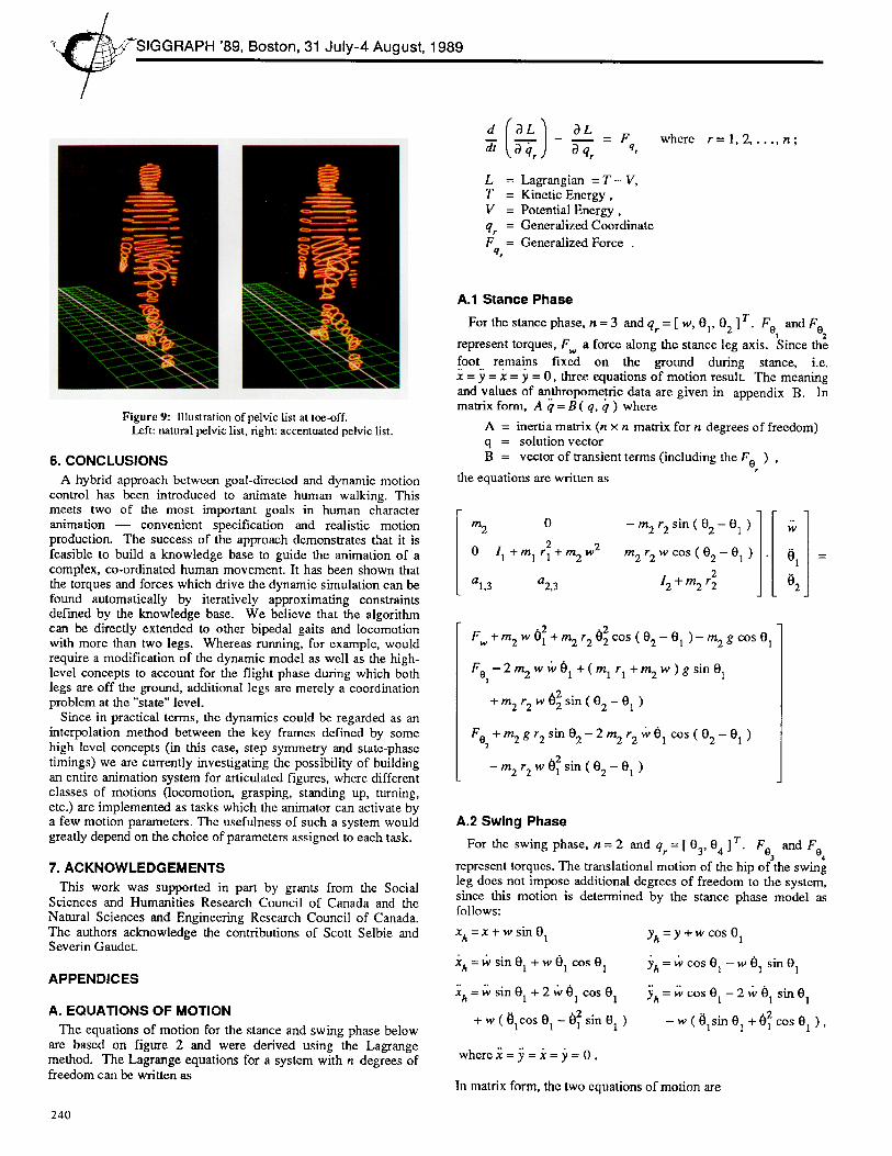
The locomotion attributes are used to individualize a walk. For instance, by changing the amount of pelvic list as shown in figure 9, significant variations of a walk are generated even for the same locomotion parameters. Figure 10 illustrates the effects of different combinations of step length and step frequency for the same the walking velocity.

The system calculates a total of 56 angles for the 37 joints of the body model - - 24 of these joints model the vertebrae in the spine - - plus a position vector in space for each time step. Currently, these computations are performed not quite in real-time; for example, it took 37.3 sec of CPU time on a SUN3-50 computer with floating point processor to compute the motion of the 12 sec walk in figure 10, top. In practice, the swing2 phase has been most expensive because of its recovery algorithm; although the duration of swing2 is only about 35 % of the time for the swing, the simulation usually takes more time than for the swing1 and swing3 phases combined. It is clear that real-time animation can be achieved by using a faster processor and by customizing the numerical integration routines.

239

'89, Boston, 31 July-4 August, 1989

dt ~ qr q"

L = Lagrangian = T - V, T = Kinetic Energy, V = Potential Energy, qr = Generalized Coordinate F = Generalized Force .

q,

where r = l , 2 . . . . . n ;

Figure 9: Illustration of pelvic list at toe-off. Left: natural pelvic list, right: accentuated pelvic list.

6. CONCLUSIONS A hybrid approach between goal-directed and dynamic motion

control has been introduced to animate human walking. This meets two of the most important goals in human character animation - - convenient specification and realistic motion production. The success of the approach demonstrates that it is feasible to build a knowledge base to guide the animation of a complex, co-ordinated human movement. It has been shown that the torques and forces which drive the dynamic simulation can be found automatically by iteratively approximating constraints defined by the knowledge base. We believe that the algorithm can be directly extended to other bipedal gaits and locomotion with more than two legs. Whereas running, for example, would require a modification of the dynamic model as well as the high- level concepts to account for the flight phase during which both legs are off the ground, additional legs are merely a coordination problem at the "state" level.

Since in practical terms, the dynamics could be regarded as an interpolation method between the key frames defined by some high level concepts (in this case, step symmetry and state-phase timings) we are currently investigating the possibility of building an entire animation system for articulated figures, where different classes of motions (locomotion, grasping, standing up, turning, etc.) are implemented as tasks which the animator can activate by a few motion parameters. The usefulness of such a system would greatly depend on the choice of parameters assigned to each task.

7. ACKNOWLEDGEMENTS This work was supported in part by grants from the Social

Sciences and Humanities Research Council of Canada and the Natural Sciences and Engineering Research Council of Canada. The authors acknowledge the contributions of Scott Selbie and Severin Gaudet.

APPENDICES

A. EQUATIONS OF MOTION The equations of motion for the stance and swing phase below

are based on figure 2 and were derived using the Lagrange method. The Lagrange equations for a system with n degrees of freedom can be written as

240

A.1 Stance Phase

For the stance phase, n = 3 and qr = [ w, 01, 02 ] T. FO 1 and Fo: represent torques, F a force along the stance leg axis. Since the foot remains fixed on the ground during stance, i.e. x = y = x = y = 0, three equations of motion result• The meaning and values of ar~thropome.trie data are given in appendix B. In matrix form, A q = B ( q, q ) where

A = inertia matrix (n x n matrix for n degrees of freedom) q = solution vector B = vector of transient terms (including the F 0 ) ,

the equations are written as

m 2 0 - m 2 r 2 sin ( 0 2 - 01 )

0 1 l + m l r ~ + m 2w 2 m 2 r 2 w c o s ( O 2 - 0 1 )

2 al,3 a2,3 I 2 + m 2 r 2 0 2

Fw + rn2 w O~ + rn 2 .2 r 2 02 cos ( 02 - 01 ) - m 2 g cos 01

Fol - 2 rn2 w ~v O 1 + ( m 1 r I + m2 w ) g sin O 1

" 2 • + m 2r 2 w 0 2 s m ( O 2 - 0 1 )

Fo2+m 2 g r E sin 0 2 - 2 m 2 r 2~,1) lCos (O 2 - 0 1 )

• 2 .

- m 2 r 2 w O 1 sm ( 0 2 - 01 )

A.2 Swing Phase

For the swing phase, n = 2 and qr = [ 03' 04 ] T. F03 and Fo4 represent torques. The translational motion of the hip of the swing leg does not impose additional degrees of freedom to the system, since this motion is determined by the stance phase model as follows:

Xh = X -t- w sin O 1

Jc h =/v sin 0 t + w 0 t cos 01

xh = ~ sin 01 + 2 ~bO 1 cos 0 t

.2 + w ( 0 1 c o s 0 1 - 0 1 sill01 )

Yh = y + w COS 01

Yh = w COS 01 -- w 01 sin 01

Y a = WC ° S 01- 2vv01 sin 01

.2 - w ( 0 1 s l n 0 1 +01 cos01 ) ,

w h e r e ~ = ~ = ~ = y = O.

In matrix form, the two equations of motion are

O ~ Computer Graphics, Volume 23, Number 3, July 1989

2 2 2 ][1 13 + m 3 r 3 +rn 4 13 14 + m 4 r4 + m 4 13 r 4 cos 04 03

+ I 4 + m 4 r42 + 2 m 4 l 3 r 4 cos 04 . =

al,2 14 + rn4 r42 04

F% + ( m 3 r 3 + m 4 l 3 ) ( xh cos 03 - Yh sin 03 )

+ m4 g4 ( xh cos ( 03 + 04 )-- Yh Sin ( 03 + O 4 )

+ m 413r 4 0 4 ( 2 0 3 + 0 4 ) s i n 0 4

- m 3 g r 3 sin 03 - m 4 g ( l 3 sin 03 + r 4 sin ( 03 + 04 ) )

Fo4+m 4 r 4(X hCOs(O 3 + 0 4 ) - y h s i l l ( 0 3 + 0 4 ) )

' 2 •

-- m 4 l 3 r 4 03 sin 04 - m 4 g r 4 sin ( 03 + 04 )

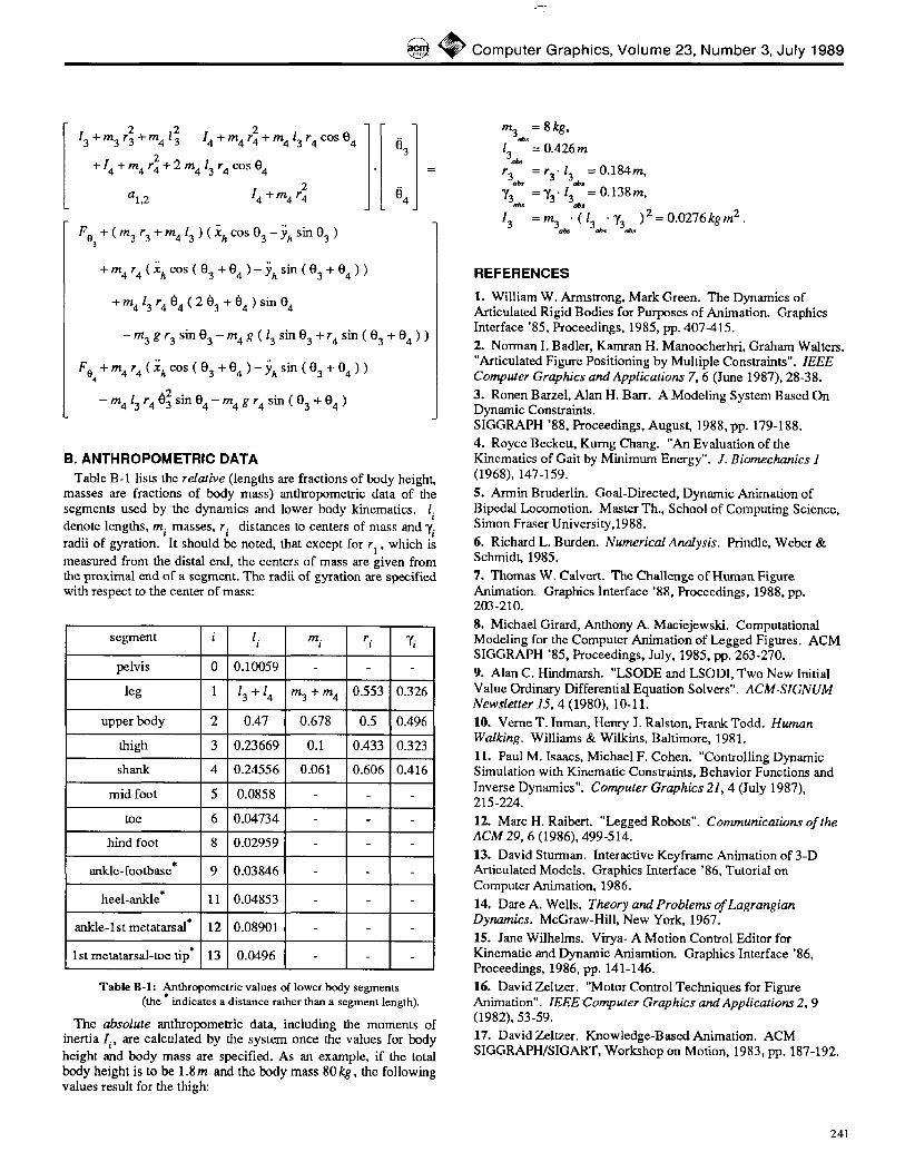
B. ANTHROPOMETRIC DATA Table B-1 lists the relative (lengths are fractions of body height,

masses are fractions of body mass) anthropometric data of the segments used by the dynamics and lower body kinematics, l i denote lengths, m i masses, r i distances to centers of mass and "Yi radii of gyration. It should be noted, that except for r l , which is measured from the distal end, the centers of mass are given from the proximal end of a segment. The radii of gyration are specified with respect to the center of mass:

segment i l i

pelvis 0 0.10059

leg 1 l 3 + 14

upper body 2 0.47

thigh 3 0.23669

shank 4 0.24556

mid foot 5 0.0858

toe 6 0.04734

hind foot 8 0.02959

ankle-footbase* 9 0.03846

heel-ankle* 11 0.04853

ankle-lstmetatarsal* 12 0.08901

lstmetatarsal-toe tip* 13 0.0496

rn i r i "Yi

m 3 + m 4 0.553 0.326

0.678 0.5 0.496

0.1 0.433 0.323

0.061 0.606 0.416

Table B-I: Anthropometric values of lower body segments (the " indicates a distance rather than a segment length).

The absolute anthropometric data, including the moments of inertia/i ' are calculated by the system once the values for body height and body mass are specified. As an example, if the total body height is to be 1.8m and the body mass 80kg, the following values result for the thigh:

rn3 ~,, = 8 kg,

13~ = 0.426 m

r3~ = r 3. 13~ = 0.184m,

Y3~ = 'Y3" 13~, = 0.138m,

13 = rn3~" ( 13~" Y3~, ) 2 = 0.0276 kg m 2 .

REFERENCES

I. William W. Armstrong, Mark Green. The Dynamics of Articulated Rigid Bodies for Purposes of Animation. Graphics Interface '85, Proceedings, 1985, pp. 407-415. 2. Norman I. Badler, Kamran H. Manoocherhri, Graham Waiters. "Articulated Figure Positioning by Multiple Constraints". IEEE Computer Graphics and Applications 7, 6 (June 1987), 28-38. 3. Ronen Barzel, Alan H. Barr. A Modeling System Based On Dynamic Constxaints. SIGGRAPH '88, Proceedings, August, 1988, pp. 179-188. 4. Royce Beckett, Kumg Chang. "An Evaluation of the Kinematics of Gait by Minimum Energy". J. Biornechanics 1 (1968), 147-159. 5. Amain Bruderlin. Goal-Directed, Dynamic Animation of Bipedal Locomotion. Master Th., School of Computing Science, Simon Fraser University,1988. 6. Richard L. Burden. Numerical Analysis. Prindle, Weber & Schmidt, 1985. 7. Thomas W. Calvert. The Challenge of Human Figure Animation. Graphics Interface '88, Proceedings, 1988, pp. 203-210. 8. Michael Girard, Anthony A. Maciejewski. Computational Modeling for the Computer Animation of Legged Figures. ACM SIGGRAPH '85, Proceedings, July, 1985, pp. 263-270. 9. Alan C. Hindmarsh. "LSODE and LSODI, Two New Initial Value Ordinary Differential Equation Solvers". ACM-SIGNUM Newsletter 15, 4 (1980), 10-11. 10. Verne T. Inman, Henry J. Ralston, Frank Todd. Human Walking. Williams & Wilkins, Baltimore, 1981. 11. Paul M. Isaacs, Michael F. Cohen. "Controlling Dynamic Simulation with Kinematic Constraints, Behavior Functions and Inverse Dynamics". Computer Graphics 21, 4 (July 1987), 215-224, 12. Marc H. Raibert. "Legged Robots". Communications o f the ACM 29, 6 (1986), 499-514. 13. David Sturman. Interactive Keyframe Animation of 3-D Articulated Models. Graphics Interface '86, Tutorial on Computer Animation, 1986.

14. Dare A. Wells. Theory and Problems of Lagrangian Dynamics. McGraw-Hill, New York, 1967. 15. Jane Wilhelms. Virya- A Motion Control Editor for Kinematic and Dynamic Aniamtion. Graphics Interface '86, Proceedings, 1986, pp. 141-146. 16. David Zehzer. "Motor Control Techniques for Figure Animation". IEEE Computer Graphics and Applications 2, 9 (1982), 53-59. 17. David Zeltzer. Knowtedge-BasedAnimation. ACM SIGGRAPH/SIGART, Workshop on Motion, 1983, pp. 187-192.

241

'89, Boston, 31 July-4 August, 1989

Figure 10: Heel-slxike for 3 walking sequences at v = 5 km/h. Top: natural walk, only v was specified, s / = 0.77 m and sf= 107.5 steps/rain were chosen by the system. Middle: short step walk, v and sl = 0.50 m were specified, sf= 166.7 steps~rain was chosen by the system. Bot tom: long step walk, v and sl = 1.05 m were specified, s f = 79.4 steps~rain was chosen by the system.

242