goals looking at data –signal and noise structure of signals –stationarity (and not)...
Post on 22-Dec-2015
215 views
TRANSCRIPT

Goals
• Looking at data– Signal and noise
• Structure of signals– Stationarity (and not)– Gaussianity (and not)– Poisson (and not)
• Data analysis as variability decomposition– Frequency analysis as variance decomposition– Linear models as variability explanation– Information-theoretic methods for variability
decomposition– …

Signal and noise
• Data analysis is about – extracting the signal that is in the noise– Demonstrating that it is ‘real’
• Everything else is details
The details
• What is the signal?
• What is the noise?
• How to separate between them?

Example: Looking at data

Example: Looking at data
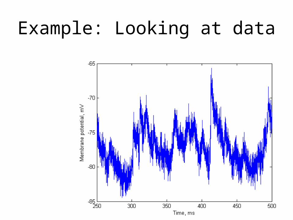
Example: Looking at data

Example: Looking at data

Example: Looking at data

Example: Looking at data

Example: Looking at data
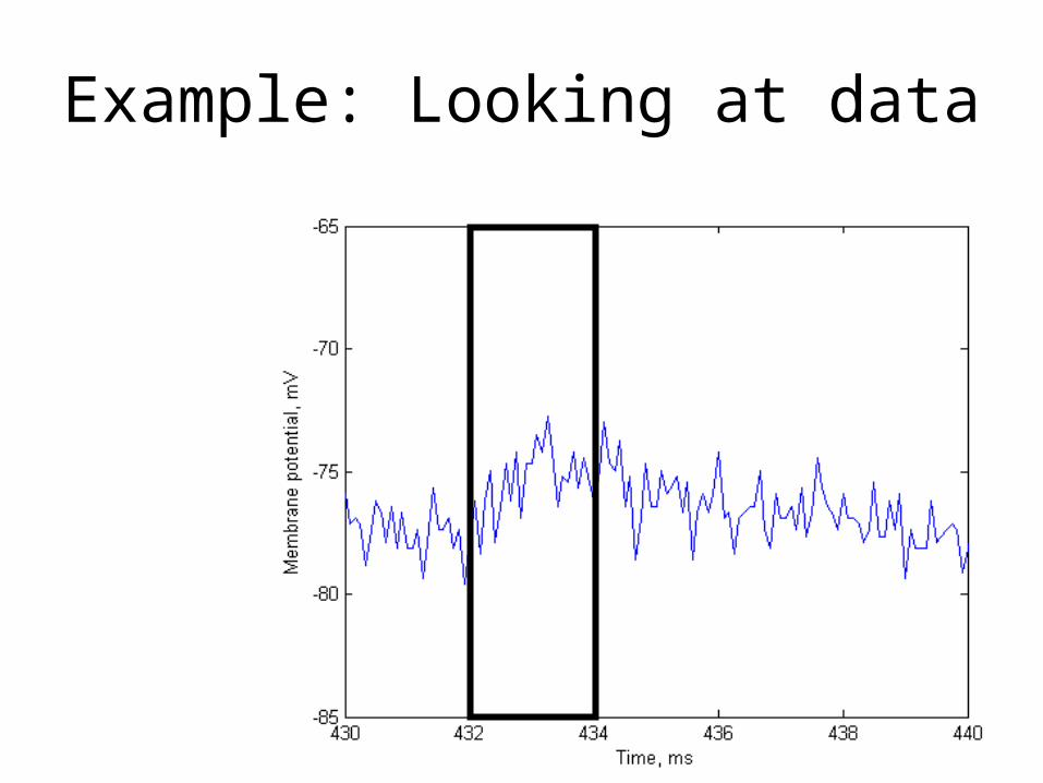
Example: Looking at data

Example: Looking at data
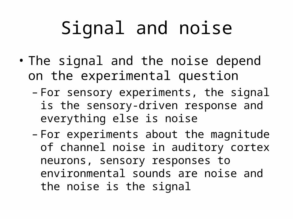
Signal and noise
• The signal and the noise depend on the experimental question– For sensory experiments, the signal is the
sensory-driven response and everything else is noise
– For experiments about the magnitude of channel noise in auditory cortex neurons, sensory responses to environmental sounds are noise and the noise is the signal
Signal and noise
• Therefore, we have to know what our signal is composed of
• The signal will have a number of sources of variability
• The experiment is about some of these sources of variability, which are then the signal, while the others are the noise

Sources of variability
• Neurobiological:– Channel noise– Spontaneous EPSPs and IPSPs– Other subthreshold voltage fluctuations
• Intrinsic oscillations• Up and down states
– Sensory-driven currents and membrane potential changes
– Spikes

Sources of variability
• Non-neuro, but biological:– Breathing, heart-rate and other motion artifacts– ERG, ECG, EMG, …
• Non-biological:– 50 Hz interference – Tip potentials, junction potentials– Noise in the electrical measurement equipment
• In the experimental part of the course, you will learn how to minimize these.

Sources of variability
• How to separate sources of variability?– By measuring them directly– By special properties
• Rates of fluctuations (smoothing and filtering)• Shape (spike clipping)
– By their timing• Event-related analysis

Fee, Neuron 2000
Direct measurement of sources of variability

Direct measurement of sources of variability
• Respiration and heart rate (for active stabilization of the electrode)
• 50 Hz interference (for removing it using event-related analysis)
• Identifying the neuron you are recording from, or at least approximately knowing the layer
• Video recording of whisker movement during recording from the barrel field in awake rats

Properties of signals
• Rates of fluctuations– Molecular conformation changes (channel
opening and closing) (may be <1ms)– Membrane potential time constants (1-30 ms)– Stimulation rates (0.1-10 s)

Nelken et al. J. Neurophysiol. 2004
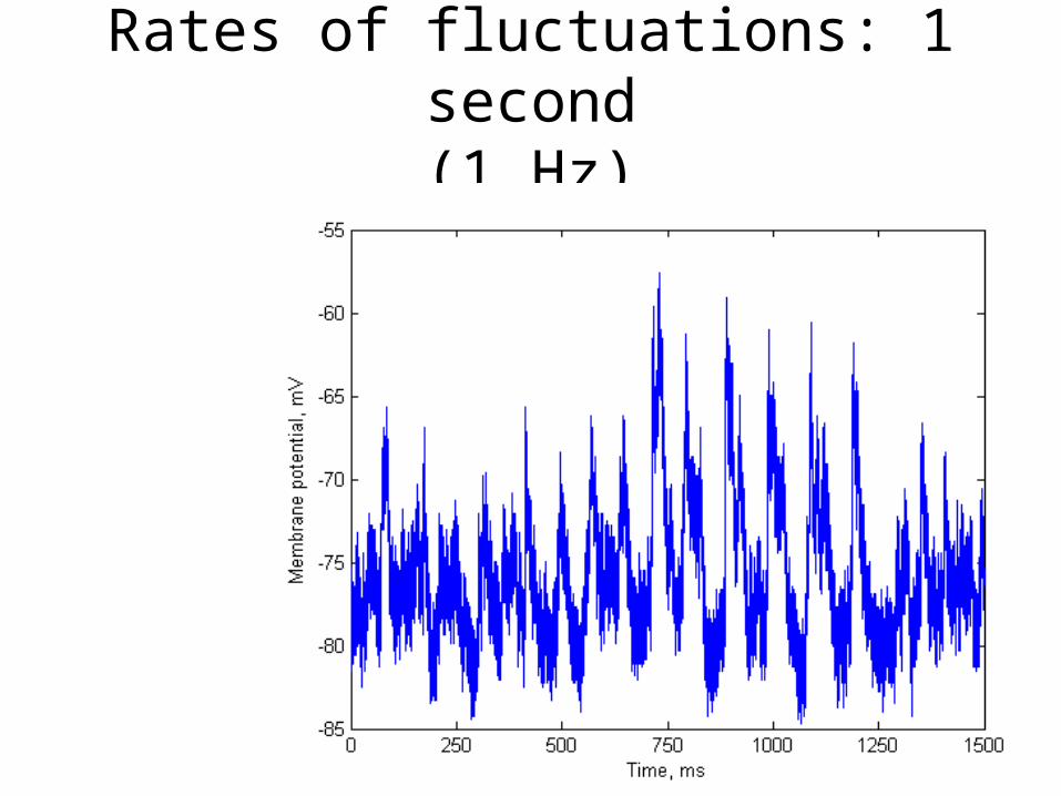
Rates of fluctuations: 1 second(1 Hz)
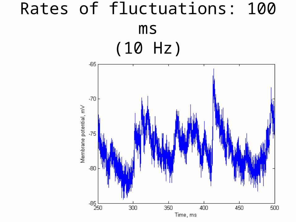
Rates of fluctuations: 100 ms(10 Hz)

Rates of fluctuations: 10 ms(100 Hz)

Rates of fluctuations: 1 ms(1 kHz)

Rates of fluctuations: 0.1 ms(10 kHz)

Rates of fluctuations
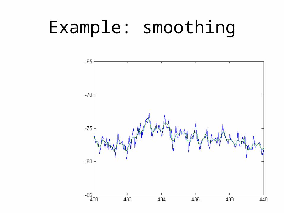
• If you know what are the relevant rates of fluctuations, you can get rid of other (faster and slower) fluctuations
• When extracting slow rates of fluctuations while removing the faster ones, this is called smoothing
• More generally, we can extract any range of fluctuations (within reasonable constraints…) by (linear) filtering

Example: smoothing

Example: smoothing

Example: smoothing

Example: smoothing
Example: smoothing
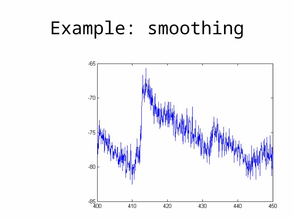
Example: smoothing

Example: smoothing

Go To Matlab
Introduction to statistical tests
• We compare two processes with the same means (0), but with obviously different variances
• We know that the variance ratio is about 4
• Is 4 large or small?

Introduction to statistical tests
• 4 is larger than 1 if the noise around 1 is such that 4 is unlikely to happen by chance

Introduction to statistical tests
• In order to say whether 4 is large or small, we would really like to compare it with the value we will get if we repeat the experiment under the same conditions
• Formally, we think of the voltage traces we compare as the result of a sampling experiment from a large set of potential voltage traces
• When possible, we would like to have a lot of examples of these potential voltage traces

Introduction to statistical tests
Many samples from up states
Many samples from down states
Filter and compute variance
Select many pairs from up states and compute ratios (should be close to 1)
Select many pairs from down states and compute ratios (should be close to 1)
Select many pairs from up and down states and compute ratios (should be close to 4)

Introduction to statistical tests
• When we have a lot of data, this is an appropriate approach
• Although note that it pushes the problem one step further (how do we know that the 1ish are indeed smaller than the 4ish)?
• But often we have only one trace, and we want to say something about it
• Need further assumptions!

Introduction to statistical tests
• Since we have only one trace, we need to invent the set from which it came
• We tend to use relatively simple assumptions about this set, which are usually wrong but not too wrong

Introduction to statistical tests
• Here we make the following two assumptions:– The two processes are stationary gaussian – The two processes have identical means
• What does that mean?– We will see later the details– We can select an independent subset of
samples from each process

Go to Matlab

Introduction to statistical tests
• Why choosing independent samples is important?
• Many years ago, people showed that ratios of sum of squares of independent, zero-mean gaussian variables with the same variance have a specific distribution, called the F distribution
• So we actually know what the expected distribution is if the variances are the same

Introduction to statistical tests
• The distribution depends on how many samples are added together (obviously…). These are called degrees of freedom, and there are two of them: one for the numerator and one for the denominator
• Here both numbers are 51
Introduction to statistical tests
• So our question got transformed to the following one:
• We got a variance ratio of 5.6, how surprising is it when we assume that the variance ratios have an F(51,51) distribution?
• In order to do that, let’s look at the F distribution…

Go to Matlab

Introduction to statistical tests
• To recapitulate:• We got data
– One trace from an up state, one trace from a down state
• We made assumptions about how many repeats should look like– Gaussian stationary with zero mean
• We generated a test for which we know the answer under the assumptions– F test (variance ratio)
• We go to the theoretical distribution and ask whether our result is extreme– Yes!
Introduction to statistical tests
• A test is as good as its assumptions…
• Are our assumptions good?
• How bad are our departures from the assumptions?

Introduction to statistical tests
• Stationarity means that – means do not depend on where they are measured– Variances and covariances do not depend on where
they are measured– …
• Gaussian processes are processes such that– Samples are gaussian– Pairs of samples are jointly gaussian (and when
stationary, the distribution depends only on the time interval between them)
– …

When the data is non-stationary?

Event-related analysis of data
• We select events that serve as ‘renewal points’
• Renewal points are points in time where the statistical structure is restarted, in the sense that everything depends only on the time after the last renewal point

Event-related analysis of data
• Examples of possible renewal points:– Stimulation times– Spike times (when you believe that everything
depends only on the time since the last spike)– Spike times in another neuron (when you
believe that …)

Event-related analysis of data
• Less obvious renewal points:– Reverse correlation analysis– The random process for which we look for
renewal points is now the stimulus– The renewal points are spike times
Event-related analysis of data
• Assume that we have renewal points in the membrane potential data
• This means that we believe that segments of membrane potential traces that start at the renewal points are samples from one and the same distribution
• We want to characterize that distribution

Event-related analysis of data
• We usually characterize the mean of the distribution
• This is called event-triggered averaging• When your event is a spike, the result is spike-
triggered averaging– If the spike is from the same neuron, the result is a
kind of autocorrelation– If the spike is from a different neuron, the result is
cross-correlation
• When your event is a stimulus, the result is the PSTH (or PSTA)

Go to Matlab

Event-related analysis of data
• We saw that using the mean does not necessarily capture well the statistics of the ensemble
• Nevertheless, mean is always the first choice because in many respects it is the simplest
• Variance and correlations are also used for event-related analysis, but this gets us beyond this elementary treatment

When the data is not gaussian?

Morphological processing
• Identifying signal events by their shape
• Usually based on case-specific methods
• Very little general theory behind it
• Closely linked to clustering

Morphological processing
• When the shapes are highly repetitive and very different from the noise, we can use matched filters
• A matched filter is a filter whose shape is precisely that of the shape to be detected

Go to Matlab

Morphological processing
• When the shapes are not necessarily highly repetitive but are still very different from the noise, we can use a generalization of matched filters
• Principal components are basic shapes whose combinations (with different weights) fit our shapes, but should poorly fit the noise
• But this takes out beyond this level…

Morphological processing
• Some spike sorting is done using principal components or matched filters
• Some EPSP identification is done using principal components
• Like all data processing techniques, this is a GIGO process and should be checked very carefully

Morphological processing
• Eventually, much of morphological processing is about deciding about classes
• You get a single number and you want to say whether it is large or small
• Some standard statistics can be used here, but mostly treatment is data-analytic