good old fashioned model theory

[Held in 120../A000-wholething.. Last changed July 26, 2004]

An introduction to

Good old fashioned model theory

[Held in 120../Preamble.. Last changed July 26, 2004]

The course will be taught

Each Tuesday from 2 – 5 pm in room J

with some lectures and some tutorial activities.The main body of course will cover the following topics.

• Basic ideas of language, satisfation, and compactness

• Some examples of elimination of quantifiers

• The diagram technique, the characterization of ∀1- and ∀2-axiomatizable theories,and similar results

• Model complete theories, companion theories, existentially closed structures, andvarious refinements

• Atomic structures and sufficiently saturated structures

• The splitting technique and ℵ0-categoricity

Depending on the time available, some of the following topics will be looked at.

• Henkin constructions

• Omiting types

• The back-and-forth technique

• Saturation methods.

Full course notes will be provided of which this is the first part.A look at the contents page will indiacte how these stand at the moment. These notes

will be modified as the course progresses.The main body of the course is contained inPart I. The extra topics are contained in Part II.

Remarks and comments in this kind of type indicate that something needs to bedone before the final version is produced.

1

Contents

Introduction . . . . . . . . . . . . . . . . . . . . . . . . . . . . . . . . . . . . . . . . . . . . . . . 70.1 Historical account–to be done . . . . . . . . . . . . . . . . . . . . . . . . . . . . . 70.2 A survey of the literature–to be re-done . . . . . . . . . . . . . . . . . . . . . . . 7

I The development 91 Syntax and semantics . . . . . . . . . . . . . . . . . . . . . . . . . . . . . . . . . . . . . . 11

1.1 Signature and language . . . . . . . . . . . . . . . . . . . . . . . . . . . . . . . . . 11Exercises . . . . . . . . . . . . . . . . . . . . . . . . . . . . . . . . . . . . . . . . . 15

1.2 Basic notions . . . . . . . . . . . . . . . . . . . . . . . . . . . . . . . . . . . . . . . 15Exercises . . . . . . . . . . . . . . . . . . . . . . . . . . . . . . . . . . . . . . . . . 18

1.3 Satisfaction . . . . . . . . . . . . . . . . . . . . . . . . . . . . . . . . . . . . . . . . 19Exercises . . . . . . . . . . . . . . . . . . . . . . . . . . . . . . . . . . . . . . . . . 22

1.4 Consequence . . . . . . . . . . . . . . . . . . . . . . . . . . . . . . . . . . . . . . . 23Exercises . . . . . . . . . . . . . . . . . . . . . . . . . . . . . . . . . . . . . . . . . 27

1.5 Compactness . . . . . . . . . . . . . . . . . . . . . . . . . . . . . . . . . . . . . . . 29Exercises . . . . . . . . . . . . . . . . . . . . . . . . . . . . . . . . . . . . . . . . . 32

2 The effective elimination of quantifiers . . . . . . . . . . . . . . . . . . . . . . . . . . . . . 332.1 The generalities of quantifier elimination . . . . . . . . . . . . . . . . . . . . . . . . 33

Exercises . . . . . . . . . . . . . . . . . . . . . . . . . . . . . . . . . . . . . . . . . 352.2 The natural numbers . . . . . . . . . . . . . . . . . . . . . . . . . . . . . . . . . . . 35

Exercises . . . . . . . . . . . . . . . . . . . . . . . . . . . . . . . . . . . . . . . . . 402.3 Lines . . . . . . . . . . . . . . . . . . . . . . . . . . . . . . . . . . . . . . . . . . . . 41

Exercises . . . . . . . . . . . . . . . . . . . . . . . . . . . . . . . . . . . . . . . . . 432.4 Some other examples – to be re-done . . . . . . . . . . . . . . . . . . . . . . . . 44

Exercises–needed . . . . . . . . . . . . . . . . . . . . . . . . . . . . . . . . . . . . . 443 Basic methods . . . . . . . . . . . . . . . . . . . . . . . . . . . . . . . . . . . . . . . . . . 45

3.1 Some semantic relations . . . . . . . . . . . . . . . . . . . . . . . . . . . . . . . . . 45Exercises . . . . . . . . . . . . . . . . . . . . . . . . . . . . . . . . . . . . . . . . . 47

3.2 The diagram technique . . . . . . . . . . . . . . . . . . . . . . . . . . . . . . . . . 47Exercises . . . . . . . . . . . . . . . . . . . . . . . . . . . . . . . . . . . . . . . . . 52

3.3 Restricted axiomatization . . . . . . . . . . . . . . . . . . . . . . . . . . . . . . . . 52Exercises . . . . . . . . . . . . . . . . . . . . . . . . . . . . . . . . . . . . . . . . . 55

3.4 Directed families of structures . . . . . . . . . . . . . . . . . . . . . . . . . . . . . . 55Exercises . . . . . . . . . . . . . . . . . . . . . . . . . . . . . . . . . . . . . . . . . 60

3.5 The up and down techniques . . . . . . . . . . . . . . . . . . . . . . . . . . . . . . 60The up technique . . . . . . . . . . . . . . . . . . . . . . . . . . . . . . . . . . . . . 61The down technique . . . . . . . . . . . . . . . . . . . . . . . . . . . . . . . . . . . 62Exercises . . . . . . . . . . . . . . . . . . . . . . . . . . . . . . . . . . . . . . . . . 63

4 Model complete and submodel complete theories . . . . . . . . . . . . . . . . . . . . . . . 654.1 Model complete theories . . . . . . . . . . . . . . . . . . . . . . . . . . . . . . . . . 65

Exercises . . . . . . . . . . . . . . . . . . . . . . . . . . . . . . . . . . . . . . . . . 674.2 The amalgamation property . . . . . . . . . . . . . . . . . . . . . . . . . . . . . . . 67

Exercises . . . . . . . . . . . . . . . . . . . . . . . . . . . . . . . . . . . . . . . . . 704.3 Submodel complete theories . . . . . . . . . . . . . . . . . . . . . . . . . . . . . . . 71

Exercises–needed . . . . . . . . . . . . . . . . . . . . . . . . . . . . . . . . . . . . . 725 Companion theories and existentially closed structures . . . . . . . . . . . . . . . . . . . . 73

5.1 Model companions . . . . . . . . . . . . . . . . . . . . . . . . . . . . . . . . . . . . 73Exercises . . . . . . . . . . . . . . . . . . . . . . . . . . . . . . . . . . . . . . . . . 76

5.2 Companion operators . . . . . . . . . . . . . . . . . . . . . . . . . . . . . . . . . . 77Exercises . . . . . . . . . . . . . . . . . . . . . . . . . . . . . . . . . . . . . . . . . 79

5.3 Existentially closed structures . . . . . . . . . . . . . . . . . . . . . . . . . . . . . . 79Exercises . . . . . . . . . . . . . . . . . . . . . . . . . . . . . . . . . . . . . . . . . 82

5.4 Existence and characterization . . . . . . . . . . . . . . . . . . . . . . . . . . . . . 82Exercises . . . . . . . . . . . . . . . . . . . . . . . . . . . . . . . . . . . . . . . . . 87

3

5.5 Theories which are weakly complete . . . . . . . . . . . . . . . . . . . . . . . . . . 87Exercises . . . . . . . . . . . . . . . . . . . . . . . . . . . . . . . . . . . . . . . . . 90

6 Pert and Buxom structures . . . . . . . . . . . . . . . . . . . . . . . . . . . . . . . . . . . 916.1 Atomicity . . . . . . . . . . . . . . . . . . . . . . . . . . . . . . . . . . . . . . . . . 91

Exercises . . . . . . . . . . . . . . . . . . . . . . . . . . . . . . . . . . . . . . . . . 976.2 Existentially universal structures . . . . . . . . . . . . . . . . . . . . . . . . . . . . 97

Exercises–needed . . . . . . . . . . . . . . . . . . . . . . . . . . . . . . . . . . . . . 1006.3 A companion operator . . . . . . . . . . . . . . . . . . . . . . . . . . . . . . . . . . 100

Exercises . . . . . . . . . . . . . . . . . . . . . . . . . . . . . . . . . . . . . . . . . 1036.4 Existence of e. u. structures . . . . . . . . . . . . . . . . . . . . . . . . . . . . . . . 103

Exercises–needed . . . . . . . . . . . . . . . . . . . . . . . . . . . . . . . . . . . . . 1087 A hierarchy of properties . . . . . . . . . . . . . . . . . . . . . . . . . . . . . . . . . . . . . 109

7.1 Splitting with Good formulas . . . . . . . . . . . . . . . . . . . . . . . . . . . . . . 110Exercises . . . . . . . . . . . . . . . . . . . . . . . . . . . . . . . . . . . . . . . . . 113

7.2 Splitting with not-Bad formulas . . . . . . . . . . . . . . . . . . . . . . . . . . . . . 113Exercises . . . . . . . . . . . . . . . . . . . . . . . . . . . . . . . . . . . . . . . . . 115

7.3 Countable existentially universal structures . . . . . . . . . . . . . . . . . . . . . . 116Exercises–needed . . . . . . . . . . . . . . . . . . . . . . . . . . . . . . . . . . . . . 117

7.4 Categoricity properties . . . . . . . . . . . . . . . . . . . . . . . . . . . . . . . . . . 117Exercises . . . . . . . . . . . . . . . . . . . . . . . . . . . . . . . . . . . . . . . . . 120

7.5 Some particular examples . . . . . . . . . . . . . . . . . . . . . . . . . . . . . . . . 121

II Construction techniques 1238 The construction of canonical models . . . . . . . . . . . . . . . . . . . . . . . . . . . . . . 125

8.1 Helpful set and its canonical model . . . . . . . . . . . . . . . . . . . . . . . . . . . 126Exercises . . . . . . . . . . . . . . . . . . . . . . . . . . . . . . . . . . . . . . . . . 132

8.2 Consistency property . . . . . . . . . . . . . . . . . . . . . . . . . . . . . . . . . . . 132Exercises . . . . . . . . . . . . . . . . . . . . . . . . . . . . . . . . . . . . . . . . . 137

9 Omitting types . . . . . . . . . . . . . . . . . . . . . . . . . . . . . . . . . . . . . . . . . . 139Exercises . . . . . . . . . . . . . . . . . . . . . . . . . . . . . . . . . . . . . . . . . 142

10 The back and forth technique . . . . . . . . . . . . . . . . . . . . . . . . . . . . . . . . . . 143Exercises . . . . . . . . . . . . . . . . . . . . . . . . . . . . . . . . . . . . . . . . . 146

11 Homogeneous-universal models . . . . . . . . . . . . . . . . . . . . . . . . . . . . . . . . . 14712 Saturation – see earlier . . . . . . . . . . . . . . . . . . . . . . . . . . . . . . . . . . . . 14813 Forcing techniques . . . . . . . . . . . . . . . . . . . . . . . . . . . . . . . . . . . . . . . . 14914 Ultraproducts–to be done . . . . . . . . . . . . . . . . . . . . . . . . . . . . . . . . . . . 150

III Some solutions to the exercises 151A For section 1 . . . . . . . . . . . . . . . . . . . . . . . . . . . . . . . . . . . . . . . . . . . 153

A.1 For §1.1 . . . . . . . . . . . . . . . . . . . . . . . . . . . . . . . . . . . . . . . . . . 153A.2 For §1.2–not yet done . . . . . . . . . . . . . . . . . . . . . . . . . . . . . . . . . 153A.3 For §1.3 . . . . . . . . . . . . . . . . . . . . . . . . . . . . . . . . . . . . . . . . . . 153A.4 For §1.4 – most not done . . . . . . . . . . . . . . . . . . . . . . . . . . . . . . . . 153A.5 For §1.5 . . . . . . . . . . . . . . . . . . . . . . . . . . . . . . . . . . . . . . . . . . 156

B For section 2 . . . . . . . . . . . . . . . . . . . . . . . . . . . . . . . . . . . . . . . . . . . 159B.1 For §2.1 . . . . . . . . . . . . . . . . . . . . . . . . . . . . . . . . . . . . . . . . . . 159B.2 For §2.2 . . . . . . . . . . . . . . . . . . . . . . . . . . . . . . . . . . . . . . . . . . 159B.3 For §2.3 . . . . . . . . . . . . . . . . . . . . . . . . . . . . . . . . . . . . . . . . . . 163B.4 For §2.4–not yet done . . . . . . . . . . . . . . . . . . . . . . . . . . . . . . . . . 164

C For section 3 . . . . . . . . . . . . . . . . . . . . . . . . . . . . . . . . . . . . . . . . . . . 165C.1 For §3.1 . . . . . . . . . . . . . . . . . . . . . . . . . . . . . . . . . . . . . . . . . . 165C.2 For §3.2 . . . . . . . . . . . . . . . . . . . . . . . . . . . . . . . . . . . . . . . . . . 165C.3 For §3.3 . . . . . . . . . . . . . . . . . . . . . . . . . . . . . . . . . . . . . . . . . . 166C.4 For §3.4 . . . . . . . . . . . . . . . . . . . . . . . . . . . . . . . . . . . . . . . . . . 166C.5 For §3.5 . . . . . . . . . . . . . . . . . . . . . . . . . . . . . . . . . . . . . . . . . . 167

4

D For section 4 . . . . . . . . . . . . . . . . . . . . . . . . . . . . . . . . . . . . . . . . . . . 169D.1 For §4.1 -to be done . . . . . . . . . . . . . . . . . . . . . . . . . . . . . . . . . . 169D.2 For §4.2 . . . . . . . . . . . . . . . . . . . . . . . . . . . . . . . . . . . . . . . . . . 169D.3 For §4.3 -no exercises yet . . . . . . . . . . . . . . . . . . . . . . . . . . . . . . 171

E For section 5 . . . . . . . . . . . . . . . . . . . . . . . . . . . . . . . . . . . . . . . . . . . 173E.1 For §5.1 . . . . . . . . . . . . . . . . . . . . . . . . . . . . . . . . . . . . . . . . . . 173E.2 For §5.2 . . . . . . . . . . . . . . . . . . . . . . . . . . . . . . . . . . . . . . . . . . 174E.3 For §5.3 . . . . . . . . . . . . . . . . . . . . . . . . . . . . . . . . . . . . . . . . . . 174E.4 For §5.4 -to be done . . . . . . . . . . . . . . . . . . . . . . . . . . . . . . . . . . 175E.5 For §5.5 . . . . . . . . . . . . . . . . . . . . . . . . . . . . . . . . . . . . . . . . . . 175

F For section 6 . . . . . . . . . . . . . . . . . . . . . . . . . . . . . . . . . . . . . . . . . . . 177F.1 For §6.1 . . . . . . . . . . . . . . . . . . . . . . . . . . . . . . . . . . . . . . . . . . 177F.2 For §6.2 -no exercises yet . . . . . . . . . . . . . . . . . . . . . . . . . . . . . . 178F.3 For §6.3 -to be done . . . . . . . . . . . . . . . . . . . . . . . . . . . . . . . . . . 178F.4 For §6.4 -no exercises yet . . . . . . . . . . . . . . . . . . . . . . . . . . . . . . 178

G For section 7 . . . . . . . . . . . . . . . . . . . . . . . . . . . . . . . . . . . . . . . . . . . 179G.1 For §7.1 . . . . . . . . . . . . . . . . . . . . . . . . . . . . . . . . . . . . . . . . . . 179G.2 For §7.2 -to be done . . . . . . . . . . . . . . . . . . . . . . . . . . . . . . . . . . 180G.3 For §7.3 -no exercises yet . . . . . . . . . . . . . . . . . . . . . . . . . . . . . . 180G.4 For §7.4 -to be done . . . . . . . . . . . . . . . . . . . . . . . . . . . . . . . . . . 180

5

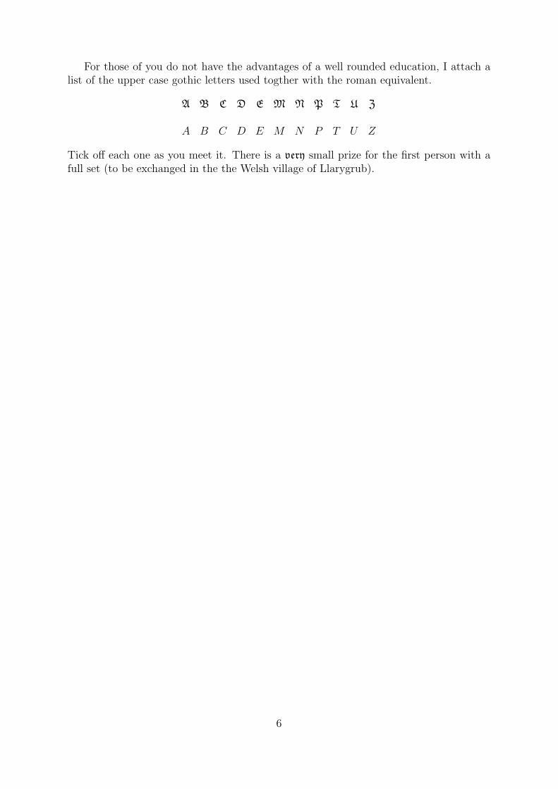
For those of you do not have the advantages of a well rounded education, I attach alist of the upper case gothic letters used togther with the roman equivalent.

A B C D E M N P T U Z

A B C D E M N P T U Z

Tick off each one as you meet it. There is a very small prize for the first person with afull set (to be exchanged in the the Welsh village of Llarygrub).

6

Introduction–to be done

0.1 Historical account–to be done

0.2 A survey of the literature–to be re-done

[Held in 120../Survey.. Last changed July 26, 2004]It seems there are few modern text that fit this introductory course. Most text are

either too old (and out of print), or cover far too much for a first course, or are on morespecialized topics.

The three articles [2], [8], and [11] of the handbook [1] form a nice introduction tothe subject. Most of the other chapters in the model theory part are also worth readingat some stage. (If you want to read any of [1], get a friend to help you pick it up. If youwant to buy [1], you will have to form a commune.)

The best introduction to model theory used to be [4]. Unfortunately I have lost mycopy, and can not locate another. From memory, I think it doesn’t cover enough for thewhole course, but it is still worth reading if you can get hold of it.

The book [3] is a bit dated, but still a good introduction. If you rip out chapters 1,5, 6, 8, 12, 13, and 14 you will have a neat little text which covers much of the course.The book [5] is from the same period, but is much more comprehensive. It suffers fromthe same defect, too much stuff on topics that are no longer central to the subject.Nevertheless, it is still worth reading.

The book [13] was written by someone who wanted to learn some model theory, andbecause of this it is a nice introductory text. It also contains a discussion of stabilitytheory (as it then stood), which is something not covered in this course but should lookedat eventually.

The best modern book on model theory is [6], but this is not for the beginner. Itcontains almost everything you need to know about model theory, much more than afirst course can contain. Unfortunately it is written in an encyclopedic rather than aprogressive form, and this makes it a bit hard for a beginner to find what he needs.Nevertheless, you should aim to become familiar with the contents of this book.

need some chat about [7]

Another book worth reading is [12]. This is an excellent introduction to many partof mathematical logic suitable for a postgraduate. It is a bit eccentric in part, not leastthat it is written in French. However, it is still worth reading. It is being translatedinto English. [This has now been translated and published -- by Springer --

so get your copies while they last]

7

[Held in 120-../A-refs.. Last changed July 26, 2004]

References

[1] J. Barwise (ed): Handbook of Mathmatical Logic, (North-Holland, 1977).

[2] J. Barwise: An introduction to first-order logic, Chapter A.1 of [1].

[3] J. L. Bell and A. B. Slomson: Models and Ultraproducts, (North-Holland, 1969).

[4] J. Bridge: Find a copy.

[5] C. C. Chang and H. J. Keisler: Model theory, (North-Holland, originally publishedin 1973 with a third edition in 1990).

[6] W. Hodges: Model Theory, (C. U. P. 1993).

[7] W. Hodges: A shorter model theory, (C. U. P. 199*).

[8] H. J. Keisler: Fundamentals of model theory: Chapter A.2 of [1].

[9] H. J. Keisler: Model theory for infinitary languages, (North-Holland, 1971).

[10] G. Kreisel and J. L. Krivine: Elements of mathematical logic, (North-Holland, 1967).

[11] A. Macintyre: Model completeness, Chapter A.4 of [1].

[12] B. Poizat: Course de Theorie des Modeles (B. Poizat, 1985).

[13] G. E. Sacks: Saturated model theory (W. A. Benjamin, 1972).

[14] C. Smorynski: Logical number theory 1, (Springer, 1991).

8

Part I

The development

This part contains the main body of thecourse as outlined in the preamble. Ofcourse, the lectures will not cover everythingin these notes, but you should try to get somefamiliarity with the whole of this material.

9

[Held in 120-../B10-bit.. Last changed July 26, 2004]

1 Syntax and semantics

Model theory (and, in fact, much of mathematical logic) is concerned, in part, with theuse of syntactic gadgetry (languages) to extract information about the objects underinvestigation. To do this efficiently we must have (at least at the back of our mind) aprecise definition of the underlying language and the associated facilities. Setting up sucha definition can look complicated, and is certainly tedious. However, the ideas involvedare essentially trivial. The role of the definition is merely to delimit what can, and whatcan’t, be done in a first order or elementary language.

In the next subsection we look at the details of this definition, and in the rest ofthis section we look at some of the consequential ramifications. Before we do that let’smotivate the ideas behind the constructions.

A structure A (of the kind we deal with in model theory) is a non-empty set A, calledthe carrier of the structure, furnished with some distinguished attributes each of which is anelement of A, a relation on A, or an operation on A. Many objects used in mathematicsare structures in this sense, but many are not. The crucial restriction here is that thestructure is single sorted with just one carrier, this carrier is non-empty, and all thefurnishings are first order over the carrier. In the wider scheme of things these are seriousrestrictions.

Often we are concerned with a whole family of structures each of the same similaritytype or signature. For such a family there is a common language which can be used totalk about any and all of these structures. This language is generated in a uniform wayfrom the signature.

This language L allows the use of the connectives

not and or implies

(and perhaps others of the same ilk). It also allows some quantification. However, in anyinstance of a quantification the bound variable can only, and must, range over the carrier(of the structure being talked about). The language allows quantification over elementsof the carrier, but not over subsets of, lists from, or any other kind of gadget extractedfrom the carrier. This is the first order restriction.

In more advanced work other kinds of languages are used, but not here. At this levelmodel theory is about the use of first order languages, and the exploitation of a centraland distinguishing result, the compactness theorem.

[Held in 120../B11-bit.. Last changed July 26, 2004]

1.1 Signature and language

In this subsection we make precise the ideas outlined above. This will take several stepsbut, as explained, there is nothing very complicated going on.

1.1 DEFINITION. A signature is an indexed family of symbols where each is either

• a constant symbol K

11

• a relation symbol R with a nominated arity

• an operation symbol O with a nominated arity

respectively. Each arity is a non-zero natural number. We speak of an n-placed relationsymbol or an n-placed operation symbol to indicate the the arity is n.

The word ‘symbol’ here indicates that eventually we will generate a formal languageL of certain strings. The letters ‘K’, ‘R’, and ‘O’ have been chosen in a rather awkwardmanner to remind us that they are syntactic symbols.

Before we start to generate the full language L let’s take a quick look at the kind ofgadget that will provide the semantics for L.

1.2 DEFINITION. A structure A for a given signature consists of the following.

• A non-empty set A, the carrier of A.

• For each constant symbol K, a nominated element A[[K]] of A.

• For each n-placed relation symbol R, a nominated n-placed relation A[[R]] on A.

• For each n-placed operation symbol O, a nominated n-placed operation A[[O]] onA.

These nominated gadgets are the distinguished attributes of A.

You should differentiate between the symbols K,R, and O of the signature and theinterpretation A[[K]],A[[R]], and A[[O]] of these in the particular structure A. There is onlyone language L of the given signature, but there are many different structures of thatsignature, each of which provides an interpretation of each symbol of the signature.

There are times in model theory when we need to take note of the size of a structure(or a language).

1.3 DEFINITION. The cardinality |A| of a structure is the cardinality |A| of it carrier.

Notice that a signature can be empty, in which case a structure (for that signature)is just a non-empty set. At the other extreme, a signature can be uncountably large.On the whole, in these notes we are concerned with signatures that have no more thancountably many relation symbols and operation symbols. However, for technical reasons,it is convenient to allow the number of constant symbols to be arbitrarily large.

1.4 DEFINITION. Given a signature, the associated primitive symbols are as follows.

• The symbols of the signature.

• The equality symbol l.

• An unlimited stock of variables v.

• The connectives ¬,∧,∨,→

• The quantifiers ∀ and ∃.

12

• The constant sentences which are true and false.

• The punctuation symbols ( and ).

There are no other primitive symbols.A string is a finite list of primitive symbols.

In other words, the primitive symbols of the language L are the symbols of the signa-ture together with a fixed collection of other symbols. These extra symbols are the samefor each language.

Again, you should not confuse the formal symbol ‘l’ (which is a primitive of eachlanguage) with the informal symbol ‘=’ used to indicate the equality of two gadgets.

A string is any finite list of primitive symbols, and can be complete gibberish

))¬v l (∧w) → ∃

or can be potentially meaningful

(∀v)(∃w)((fvw l v) ∧ ¬(fwv l w))

(where v, w are variables and f is a 2-placed operation symbol). Our aim is to extractthe potentially meaningful strings.

We do that in three steps. We define the terms t, the atomic formulas θ, and then theformulas φ. The formulas are the potentially meaningful strings. Each of these strings

t θ φ

has an associated support∂t ∂θ ∂φ

giving the set of variables occurring freely in the string. The support is generated at thesame time as the parent string.

1.5 DEFINITION. Each signature has an associated set of terms and each such term thas an associated set ∂t of free variables. These are generated as follows.

• Each variable v is a term, and ∂v = v.

• Each constant symbol K is a term, and ∂K = ∅.

• For each n-placed operation symbol O and each list t1, . . . , tn of terms, the com-pound

(Ot1 · · · tn)

is a term and∂(Ot1, · · · tn) = ∂t1 ∪ · · · ∪ ∂tn

is its set of free variables.

There are no other terms.

Notice that each term can be uniquely parsed (so that its construction can be displayedas a finite tree). That is the job of the brackets in the construction.

13

1.6 DEFINITION. For a signature the atomic formulas are those strings

true false (t1 l t2) (Rt1 · · · tn)

where t1, t2, . . . tn are terms and R is an n-placed relation symbol. Each such atomicformula θ has a set ∂θ of free variables given by

∅ ∅ ∂t1 ∪ ∂t2 ∂t1 ∪ · · · ∪ ∂tn

respectively.

Notice the difference between

(t1 = t2) (t1 l t2)

where t1, t2 are terms. The first asserts that the two terms are the same (that is, the samestring of primitive symbols), whereas the second is an atomic formula of the languagewhich, in isolation, has no truth value.

Finally we can extract the potentially meaningful strings.

1.7 DEFINITION. Each signature has an associated set of formulas and each such formulaφ has an associated set ∂φ of free variables. These are generated as follows.

• Each atomic formula is a formula with free variables, as given.

• For each formula ψ the string ¬ψ is a formula with ∂¬ψ = ∂ψ.

• For each pair θ, ψ of formulas, each of the strings

(θ ∧ ψ) (θ ∨ ψ) (θ → ψ)

is a formula with free variables∂θ ∪ ∂ψ

in each case.

• For each formula ψ and variable v, each of the strings

(∀v)ψ (∃v)ψ

is a formula with free variables∂ψ − v

in both cases.

There are no other formulas.

Notice that once again each formula can be uniquely parsed.The language L given by a signature is the set of all formulas associated with that

signature. In practice we usually don’t even mention the signature, but use phrases suchas

structure suitable for the language Lterm of the language Lformula of the language L

and so on.In a way the formulas are not the most important strings associated with a signature.

14

1.8 DEFINITION. A sentence of a language is a formula σ of that language with no freevariables, ∂σ = ∅.

Sentences are those strings which are either true or false in any particular structure.Formulas are really just a stepping stone in the construction of sentences.

It may not be clear what role the two contant sentences true and false play.At times it is convenient to have a sentence which is trivially valid in every structure

we meet and, as a string, is very simple. If the language has a constant K, then (K l K)is such a sentence. However, sometime there isn’t a contant around, and then we haveto look elsewhere. We could take the sentence (∀v)(v l v), but that quantifier can bea nuisance. The primitive true is there so that we always have such a trivially true andsimple sentence. The primitive false palys a similar role, except this one is a triviallyfalse and simple sentence.

Finally, for this subsection, as indicated above we want to measure the size of alanguage.

1.9 DEFINITION. The cardinality |L| of a language L is either ℵ0 or the size of thesignature, whichever is the larger.

The cardinal |L| is infinite. If the signature is finite or countable, then |L| = ℵ0,otherwise it is the cardinality of the signature. For the most part we will be interestedin countable languages. However, even for such a language, one of the most commontechniques of model theory involves the use of associated languages of larger cardinality.Thus we have to deal with the general case.

Exercises

1.1 Consider the signature with just one symbol < which is a 2-placed relation symbol.We write this as an infix. Let u, v be a pair of distinct variables and set

φ0 := (v l v) θr := (∃v)[(u l v) ∧ φr] φr+1 := (∃u)[(u < v) ∧ θr]

for each r < ω to obtain two ω-chains of formulas.(a) Write down φ0, φ1, φ2, and perhaps φ3 until you can see what is going on.(b) Calculate ∂φr and ∂θr for each r < ω.(c) Describe a different way of setting up equivalent formulas which makes the uses

of the variables easier to see.


1.2 Basic notions

In subsection we gather together a few more basic notions and some conventions whichmake the day to day handling of formulas a little less tedious.

We begin with the simplest comparison between two structures.

15

1.10 DEFINITION. Given a pair A,B of structures (for the same language), we write

A ⊆ B

and say A is a substructure of B or B is a superstructure of A, if the following hold.

• The carrier A of A is a subset of the carrier B of B.

• For each constant symbol K of the signature, A[[K]] = B[[K]].

• For each n-placed relation symbol R of the signature, the relation A[[R]] is therestriction to A of the relation B[[R]]. In other words,

A[[R]]a1 · · · an ⇐⇒ B[[R]]a1 · · · an

holds for each a1, . . . , an ∈ A.

• For each n-placed relation symbol O of the signature, the set A is closed underB[[O]], and the operation A[[O]] is the restriction to A of the operation B[[O]]. Inother words

A[[O]]a1 · · · an = B[[O]]a1 · · · an

holds for each a1, . . . , an ∈ A.

In short, A is closed under the attributes of B, and these give the attributes of A.

Thus, given a structure B, each substructure A is completely determined by its carrier.However, not every subset of the carrier of B is the carrier of a substructure.

In subsection 3.1 we will look at a generalization of this idea. We define the notionof an embedding

Af

- B

of a structure into another using a function f between the carriers. When this functionis an insertion we obtain A ⊆ B.

Two structures A,B (of the same language) are isomorphic

A ∼= B

if there is an isomorphism from one to the other. This is a bijection between the carrierswhich matches the distinguished attributes. We needn’t write down the precise detailsof this, for it is a particular case of an embedding (which we look at later). However, wewill use the notion.

Each language L consists of a set of formulas, some of which are sentences. Often weare interested in particular kinds of formulas, ones of a certain ‘complexity’. The mostcommon measure of formulas is by quantifier complexity.

There are various useful classifications of formulas. Let’s look at two of these, one ofwhich builds on top of the other.

Let L be an arbitrary language.

• An atom is just an atomic formula, as in Definition 1.6.

16

• A literal is an atom α or the negation ¬α of an atom.

• A formula δ is quantifier-free if it contains no quantifiers, no uses of ∀ or ∃.

Each quantifier-free formula δ can be rephrased in one of two useful normal forms.

• The conjunctive normal form in which δ is rephrased as a conjunction

D1 ∧ · · · ∧Dm

of disjuncts each of which is a disjunction of literals.

• The disjunctive normal form in which δ is rephrased as a disjunction

C1 ∨ · · · ∨ Cm

of conjuncts each of which is a conjunction of literals.

Here ‘rephrased’ means ‘is logically equivalent to’. The standard boolean manipulationof formulas enables us to move from δ to either of the normal forms.

In the same way, using the rules for manipulating quantifiers, we know that eachformula can be rephrased in prenex normal form as

(Q1v1) · · · (Qnvn)δ

where each Q in the prenex is a quantifier and the matrix δ is quantifier-free. By takingnote of the alternations in the prenex we obtain the quantifier hierarchy of formulas.

∀1 ∀2 ∀3

AAAAAAAA

A

AAAAAAA

QF · · ·@

@@

∃1 ∃2 ∃3

Thus ∀0 = ∃0 = QF is the set of formulas each of which is logically equivalent to aquantifier-free formula. For each n ∈ N the sets

∀n+1 ∃n+1

consists of the formulas logically equivalent to

(∀v1, . . . , vn)φ (∃v1, . . . , vn)φ

whereφ ∈ ∃n φ ∈ ∀n

respectively. Inclusions between these sets are indicated in the diagram.As you can imagine, handling formulas can be a bit tedious especially if we stick

strictly to the letter of the law.

17

When we display a particular formula we often leave out some of the brackets or usedifferent shapes of brackets to make the formula more readable. There are one or twoother tricks we sometimes use.

Each formula φ has an associated set ∂φ of free variables. We often write

φ(v1, . . . , vn)

to indicate that ∂φ = v1, . . . , vn. Notice that at this level we are not concerned withthe order or number of occurrences of each free variable in φ. In fact, a variable camoccur freely and bound in the same formula. Exercise 1.1 gives an extreme example ofwhat can happen.

For much of what we do any finite list of variables can be treated as a single variable.We use some informal conventions to handle this. Thus we often write

φ(v)

to indicate that v is a listv1, . . . , vn

of variables each of which occurs freely in φ. Thus, in this usage

φ(v) φ(v1, . . . , vn)

mean the same thing. There is, of course, plenty of scope for confusion here. However,we will always make this situation clear.

In the same way we sometimes write

(∀v)φ(v) for (∀v1, . . . , vn)φ(v1, . . . , vn)

when the number of variables in the list v is not important.As well as single formulas we also use sets of formulas. Let Γ be such a set of formulas,

and consider∂Γ =

⋃∂φ |φ ∈ Γ

the set of all variables that occur free somewhere in Γ. This could be an infinite set.Often we restrict this support.

1.11 DEFINITION. A type is a set Γ of formulas such that ∂Γ is finite.

Do not confuse this use of the word ‘type’ with other uses. Some of these have norelationship at all with this usage.

Exercises

1.2 Consider the following three posets.

A B C

carrier A = a, b B = a, b, c D = a, b, c, dcomparisons a ≤ b a ≤ b ≤ c d ≤ a ≤ c, d ≤ b ≤ c

Draw a picture of each and determine those pairs of structures where one is a substructureof the other.


18

1.3 Satisfaction

Having made the effort to set up the notion of the language L suitable for structures A

of some given signature, and in which the idea of a sentence σ is made precise, it is nowpatently obvious what

the structure A satisfies σ

means. The whole of the rather tedious construction of L was driven with this in mind.Nevertheless, it is worth looking at the formal definition of this notion (not least becausesome people think that it has some content). In more advanced work various non-elementary languages are used, and then the internal workings of the language and itssatisfaction relation are more important.

We are talking about the pivotal notion of model theory, so we can’t keep writing itout in words. Accordingly we let

A |= σ

abbreviate the phrase above (A satisfies σ). This, of course, is a relation between struc-tures A and sentences σ, so each instance is either true or false. This truth value isgenerated by recursion on the construction of σ. That is, we define outright the value forsimple sentences, and then show how to obtain the value for compound sentences fromthe values for its components. This brings out a minor snag.

As we unravel the construction of σ, we will meet certain formulas, and these maycontain free variables. But such variables have no interpretation in A. They are merely alinguistic device to indicate certain bindings in larger formulas. However, to push throughthe recursion, we need to show what to do with any free variables that arise as we unravelthe sentence σ. We use a little trick.

1.12 DEFINITION. For a structure A, an A-assignment is a function x which attaches toeach variable v an element vx of A.

(Notice that although we call x a function, we write its argument v on the left.)The idea is that if we meet a free variable v which, apparently, has no interpretation,

then we give it the value vx. Before we see how this helps with the satisfaction relation,let’s look at a similar use in a simpler situation.

Each term t (of the underlying language L) is built from certain constants K, certainoperation symbols O, and certain free variables v. How can we give t a value in somestructure A? We have interpretations A[[K]] and A[[O]] of K and O, but we have nointerpretation of v. To get round this we use an assignment x, and define the value of tin A at x.

1.13 DEFINITION. For each structure A (suitable for a language L), each A-assignmentx, and each term t (of L) the element

A[[t]]x

of A is generated by recursion on the construction of t using the following clauses.

• If t is a variable v thenA[[t]]x = vx

using the element assigned to v by x.

19

• If t is a constant symbol K then

A[[t]]x = A[[K]]

(the interpretation of K in A).

• If t is a compound(Ot1 . . . tn)

where O is an n-placed operation symbol and t1, . . . , tn are smaller terms, then

A[[t]]x = A[[O]]a1 · · · an

whereai = A[[ti]]x

for each 1 ≤ i ≤ n.

No other clause are required.

There is nothing in this definition. Each term t names, in an obvious way, a certain(compound) operation on (the carrier of) A. This construction merely evaluates thisoperation, in the obvious way, where the inputs are supplied by the assignment x. Inparticular, for each term t almost all of the assignment x is not needed.

1.14 LEMMA. Let A be a structure and let t be a term (of the underlying language). Ifx and y are A-assignments which agree on ∂t, that is if

vx = vy

holds for each v ∈ ∂t, thenA[[t]]x = A[[t]]y

holds.

This is proved by the obvious induction over the construction of t.To generate the satisfaction relation we use the same trick. We define a more general

relationA |= φx

which says

A satisfies the formula φ where each free variable v takes the value vx

and then we show the irrelevancy of most of x in Lemma 1.16.

1.15 DEFINITION. For each structure A (suitable for a language L), each A-assignmentx, and each formula φ (of L) the truth value

A |= φx

20

is generated by recursion on the structure of t using the following clauses.

A |= (true)x ⇐⇒ true

A |= (false)x ⇐⇒ false

A |= (t1 l t2)x ⇐⇒ A[[t1]]x = A[[t2]]x

A |= (Rt1 · · · tn)x ⇐⇒ A[[R]]a1 · · · an where ai = A[[ti]]x

A |= (¬ψ)x ⇐⇒ not(A |= ψx)

A |= (θ ∧ ψ)x ⇐⇒ A |= θx and A |= ψx

A |= (θ ∨ ψ)x ⇐⇒ A |= θx or A |= ψx

A |= (θ → ψ)x ⇐⇒ not(A |= θx) or A |= ψx

A |= ((∀v)ψ)x ⇐⇒ A |= ψyfor each A-assignment ywhich agrees with x exceptpossibly in the v-position

A |= ((∃v)ψ)x ⇐⇒ A |= ψyfor some A-assignment ywhich agrees with x exceptpossibly in the v-position

No other clauses are required.

Notice thatA |= (true)x

always holds, whereasA |= (false)x

never holds. This is the principal job of these two constant sentences.To get the original satisfaction relation (for sentences) we make the following obser-

vation.

1.16 LEMMA. Let A be a structure and let φ be a formula (of the underlying language).If x and y are A-assignments which agree on ∂φ, that is if

xx = vy

holds for each v ∈ ∂φ, thenA |= φx ⇐⇒ A |= φy

holds.

By definition, a sentence is a formula σ with ∂σ = ∅. Vacuously, for such a sentence,each two A-assignments x and y agree on ∂σ, and hence

A |= σx ⇐⇒ A |= σy

holds. In other words, eitherA |= σx

for every A-assignment or for no A-assignment. Thus, we may write

A |= σ

21

to indicate that A |= σx holds for every x.In a similar way we may simplify the notation A |= φx.Consider a formula φ(v1, . . . , vn), that is a formula φ with ∂φ = v1, . . . , vn. Given

a structure A and an assignment x, the truth value of

A |= φx

depends only on the elements

a1 = v1x, . . . , an = vnx

selected from x by the free variables. Thus we often write

A |= φ(a1, . . . , an)

in place of the official notation.Sometime we go even further. By a point a of the structure A we mean a list a1, . . . , an

of elements of A. We may then write

A |= φ(a)

for the satisfaction relation. Of course, this assumes there is a match between the pointa and the list v of free variables of φ.

In subsection 1.2 we introduced the idea of isomorphic structures

A ∼= B

(of the same signature). There is a semantic analogue of this.We write

A ≡ B

and say A and B are elementarily equivalent if

A |= σ ⇐⇒ B |= σ

holds for each sentence σ (of the underlying language). Almost trivially

A ∼= B =⇒ A ≡ B

holds (but the proof of this is rather tedious). However, the converse is false (in general).In fact, as we will see in Theorem 1.27, it can happen that A ≡ B but |A| 6= |B| and sothese structures can’t be isomorphic.

Exercises

1.3 Sketch the proofs of Lemmas 1.14 and 1.16.

1.4 Consider the formulas φr generated in Exercise 1.1, and let N = (N, <).(a) Characterize the elements a of N such that N |= φr(a).(b) Show that N |= (∀v)[φr+1 → φr] holds for each r < ω.(c) Describe the formulas ψ(v) such that N |= (∀v)[ψ → φr] holds for each r < ω.

22

1.5 Consider the language on the empty signature. In other words, consider the languageof pure equality.

(a) Show that for each n < ω there are sentences σn and τn such that

A |= σn ⇐⇒ |A| ≥ n A |= τn ⇐⇒ |A| = n

holds for each structure A. What is the quantifier complexity of each of these sentences?(b) Show there is a set Inf of sentences such that

A |= Inf ⇐⇒ A is infinite

holds for each structure A. Is there a finite set of such sentences?(c) Is there a set Fin of sentences such that

A |= Fin⇐⇒ A is finite

for each each structure A?

1.6 Suppose A ⊆ B.Show that

A |= δ(a) ⇐⇒ B |= δ(a)

for each quantifier-free formula δ(v) and point a of A which matches the free variables vof δ.

Show thatA |= θ(a) =⇒ B |= θ(a)

for each ∃1-formula θ(v) and point a of A which matches the free variables v of θ.Find an example to show that this implication is not an equivalence.


1.4 Consequence

Each language L has an associated satisfaction relation

A |= σ

between structures A (for L) and sentences σ (of L). We can refine this.

1.17 DEFINITION. Let L be a language, let K be a class of structures for L, and let Σbe a set of sentences of L.

(a) The relationK |= Σ

holds ifA |= σ

holds for each A ∈ K and σ ∈ Σ.(b) The theory Th(K) of K is the set of all sentences σ such that K |= σ.(c) The models M(Σ) of Σ is the class of all structures A such that A |= Σ.

23

The two assignments M(·) and Th(·) form a galois connection. Thus

K ⊆M(Σ) ⇐⇒ Σ ⊆ Th(K)

holds for each class K (of structures) and each set Σ (of sentences). Furthermore, eitherside holds precisely when

K |= Σ

holds. In particular, both the composites Th M and M Th are closure operationsand, as expected, we look at the closed gadgets.

1.18 DEFINITION. (a) A set T of sentences is a theory if T = Th(K) for some class K ofstructures. Equivalently, T is a theory if (and only if) T = Th(M(T )).

(b) A class K of structures is elementary or an elementary class if K = M(Σ) for someset Σ of sentence. Equivalently, K is elementary if (and only if) K = M(Th(K)).

These notions prompt some obvious questions.

• Are there any necessary and sufficient conditions for a class to be elementary?

• By definition, a class is elementary if it has the form M(Σ) for a set Σ of sentences.When is a class strictly elementary, that is when does it have the form M(σ) for asingle sentence?

• What are the necessary and sufficient conditions for a set of sentences to be atheory?

• By definition, a set T is a theory if it has the form Th(M(Σ)) for some set Σ. Wethen say Σ axiomatizes T . When does a theory have a finite set of axioms? Whenis a theory ∀n-axiomatizable for some n?

To answer these and similar questions we need a tool, the compactness theorem. Thisis the pivotal method of model theory, and is discussed in detail in the next subsection.Here we see how it relates to another part of mathematical logic.

1.19 DEFINITION. A set Σ of sentences (of some language) is consistent or satisfiable ifit has a model, that is if A |= Σ for some structure A.

The theory T is inconsistent (not consistent) if T = Th(∅), in which case T is the setof all sentences of the language. Rarely do we need to consider this theory, so we oftensay ‘a theory T ’ when we mean ‘a consistent theory T ’.

1.20 DEFINITION. A theory T is complete if it is consistent and A ≡ B for all modelsA,B of T .

A theory T is κ-categorical (for a cardinal κ) if A ∼= B for all models A,B of T with|A| = κ = |B|.

It is an easy exercise to see that a theory is complete if and only if it has the formTh(A) for a structure A. Another easy exercise (but using a result we haven’t yet seen)shows that if a consistent theory T in in a language L is κ-categorical for some κ ≥ |L|,then it is complete.

Roughly speaking a complete theory is a large theory in the sense that it can’t takein any more sentences without becoming inconsistent. At the other extreme, the purelogic of a language it the theory of the class of all structures for that language. Thus asentence belongs to this theory if and only if it is universally valid.

24

1.21 DEFINITION. For a set Σ of sentences and a sentence σ we write

Σ ` σ

and say Σ entails σ or σ is a consequence of Σ if σ ∈ Th(Σ), that is if A |= σ for eachmodel A |= Σ.

In this notation Σ is a set of axioms for a theory T exactly when

σ ∈ T ⇐⇒ Σ ` σ

holds for each sentence σ. Often we describe a theory by writing down a particular setof axioms. Then one of the problems is to characterize all (or a large amount of) theconsequences of the axioms. At other times the problem can be to axiomatize the theoryof some given class of structures (which is described in a non-elementary way).

Although it is not strictly part of model theory, at this point it is worth comparingthis semantic consequence relation with the kind of consequence relation met in a courseon predicate calculus.

The Definition 1.21 of the relation ` involves an external quantification over a po-tentially large class of structures. The relation Σ ` σ holds if . . . for all structuresA. However, Σ ` σ is a relation between syntactic objects, and the question arises ofwhether it can be characterized in purely combinatorial terms.

Godel’s completeness theorem shows that it can.(You should not confuse the two different uses of ‘completeness’ here. They are

related, but not the same.)To analyse ` we first set up a proof-theoretic relation

Σ ˙ σ

between sets Σ of sentences and sentences σ. The essential feature of this is that itis entirely combinatorial. This relation holds if and only if there is a certain (finite)configuration of strings of symbols. The intended semantics is not referred to at all.Thus, Σ ˙ σ can be shown to hold by exhibiting a certain collection of symbols formattedin an appropriate way.

There are several different ways of setting up ˙ , most of which are needed for onejob or another (and some of which are entirely untainted by content and interest). Herewe needn’t worry about the precise details.

The analysis now investigates the relationship between

˙ `

to produce two particular results, one minor and one major.

• The relation ˙ is sound, that is

Σ ˙ σ =⇒ Σ ` σ

holds for all Σ and σ. This is a relatively trivial observation.

25

• The relation ˙ is adequate, that is

Σ ` σ =⇒ Σ ˙ σ

holds for all Σ and σ. This requires quite a bit of work.

• The combination of these two results is the completeness theorem, that is

Σ ` σ ⇐⇒ Σ ˙ σ

holds for all Σ and σ.

Because of the way ˙ is set up we observe that if

Σ ˙ σ

thenΓ ˙ σ

for some finite part Γ of Σ. This leads to the following result.

1.22 THEOREM. Let Σ be a set of sentences (in some language). If each finite part ofΣ has a model, then Σ has a model.

Proof. We prove the contrapositive. Thus suppose Σ does not have a model. Then,vacuously we have

Σ ` σ

for each sentence σ. Consider the sentence false which does not have a model. We have

Σ ` false

and henceΣ ˙ false

by the adequacy of ˙ . But nowΓ ˙ false

for some finite part Γ of Σ, and then

Γ ` false

by the soundness of ˙ . This shows that Γ does not have a model.

This result is a version of the compactness theorem.

26

Exercises

The first two exercises are concerned with the language with just one attribute, and thatis a binary relation symbol. Thus a structure for this language has the form (A,R) whereA is a non-empty set and R is binary relation on A.

1.7 An equivalence structure has the form (A,R) where R is an equivalence relation onthe carrier A.

(a) Axiomatize the class of equivalence structures.(b) For m,n < ω, axiomatize the class of equivalence structures each having no more

than m equivalence classes, and each of these has no more than n members.(c) Axiomatize the class of equivalence structures having infinitely many equivalence

classes and each of these is infinite.(d) Axiomatize the class of equivalence structures which are such that if there is a

finite equivalence class, then there is an equivalence class of each larger finite size.

1.8 (a) Axiomatize the classes of posets, linear orderings, dense linear orderings, anddiscrete linear orderings.

(b) Write down formulas θ(u, v, w), ψ(u, v, w), φ(u, v) such that

A |= θ(a, b, c)⇐⇒ c is the l.u.b. of b and c

A |= ψ(a, b, c)⇐⇒ a, b, c are linearly ordered in A

A |= φ(a, b) ⇐⇒if a, b are comparable and not equal, then exactlythree elements lie strictly between a, b, and thesethree elements are pairwise incomparable

hold for each poset A and elements a, b, c of A.

The next exercise uses the language suitable for structures

A = (A, ∗, e)

where ∗ is a binary operation on A and e is a distinguished element.

1.9 (a) Axiomatize the classes of groups, abelian groups, torsion-free abelian groups,and divisible abelian groups. Which of these classes are finitely axiomatizable.

Write down formulas θ(u), ψ(u, v), φ(u, v) such that

A |= θ(a) ⇐⇒ a is a commutator

A |= ψ(a, b)⇐⇒ a is in the centralizer of b

A |= φ(a, b)⇐⇒ there is an inner automorphism taking a to b

for each group A and elements a, b of A.

1.10 By using a suitable signature axiomatize the classes of rings (with 1), commutativerings (with 1), integral domains, integral domains of characteristic p (where p is a prime),integral domains of characteristic 0, fields, algebraically closed fields.

Which of the classes are ∀2-axiomatizable, ∀1-axiomatizable, finitely axiomatizable?

27

1.11 Consider the reals as a structure (R,+,×,≤, 0, 1) (with the obvious attributes.Look up the axioms which characterize this structure up to isomorphism. Observe thatmost of these are first order, but the crucial one isn’t. What is this non-elementaryaxiom?

1.12 Let R be a ring with 1, and consider the right R-modules. Think of each of theseas a structure

A = (A,+, 0, (fr | r ∈ R))

where (A,+, 0) is an abelian group and, for each r ∈ R, the 1-placed operation fr isa 7→ ar. Thus R is used to index part of the signature.

Write down axioms for this class of modules.What changes need to be made to axiomatize the class of left R-modules?

1.13 Show that for each consistent theory T the following are equivalent.(i) T is complete(ii) For each sentence σ, if T ∪ σ is consistent, then σ ∈ T .(iii) For each theory T ′, if T ⊆ T ′ then either T = T ′ or T ′ is inconsistent.(iv) For each pair σ, τ of sentences, if σ ∨ τ ∈ T , then σ ∈ T or τ ∈ T .

The following exercise is quite tricky, but it solution uses an important techniquewhich you should learn as soon as possible.

1.14 Show that if no finite extension of a (consistent) theory is complete, then the theoryhas at least 2ℵ0 complete extensions.

Finally, here is almost all you need to know about galois connections.

1.15 Let A, S be a pair of posets with elements a, b, c, . . . and r, s, t, . . ., respectively. Let

A]

- S A [

S

be a pair of assignments such that

a ≤ [s⇐⇒ s ≤ ]a

holds for each a ∈ A and s ∈ S.(a) Show that both the composites [ ] and ] [ are inflationary.(b) Show that ] [ ] = ] and [ ] [ hold.(c) Show that both [ and ] are antitone.(d) Show that both [ ] and ] [ are closure operations.

[Held in 120.../B15-bit... Last changed July 26, 2004]

28

1.5 Compactness

At the end of the previous subsection we obtained a statement (and an indication of aproof) of the compactness theorem. In this subsection we take a closer look at this result.

1.23 DEFINITION. A set Σ of sentences (of some language) is consistent or satisfiable ifit has a model, that is if A |= Σ for some structure A.

A set Σ of sentences is finitely satisfiable if each finite part has a model.

In this terminology, we saw that the completeness theorem implies the following.

1.24 THEOREM. (The crude compactness theorem) If a set of sentences (of some lan-guage) is finitely satisfiable, then it is satisfiable.

How should we prove this?We have seen already one method of proof. We set up a proof-theoretic consequence

relation ˙ and then prove a completeness result. The compactness result is an immediateconsequence. However, this is not entirely satisfactory, for two reasons.

Firstly, we must set up all the machinery for ˙ , and this takes some time. Further-more, this machinery is never used again in model theory. (It may be used elsewherein mathematical logic, but then ˙ will be the principal object of study, and it will bedesigned with some specific class of tasks in mind.)

Secondly, at the heart of the proof of completness a certain structure is constructed.The method of construction can be modified to give a direct proof of compactness (with-out a detour through ˙ and its properties).

The witnessing construction is described in section 8. This is a method of producinga structure out of a certain kind of family of sets of sentences (called a consistency prop-erty). In the first instance this construction gives us both compactness and completeness,virtually by the same proof. This method of construction is quite flexible, and gives usquite a lot of control over the end product. This is used to advantage in more advancedwork. Furthermore, the same method can be lifted to higher order languages (but, ofcourse, this requires a bit more work).

Another idea on how to prove compactness should have occurred to you.Let Σ be a finitely satisfiable set of sentences, and let ∆ be the set of finite subset

∆ of Σ. We are given a model A(∆) of each such ∆ ∈ ∆. Is there a way of patchingtogether, in a coherent fashion, all of these A(∆) to produce a model of Σ? There is, andit is called the ultraproduct construction. This is described in section 14.

For the time being we do not need the details of the proof of Theorem 1.24, so let’slook at some applications of compactness.

1.25 THEOREM. Let L be any language.(a) The class of all infinite structures (for L) is elementary but not strictly elementary.(b) The class of all finite structures is not elementary.(c) A sentence (of L) holds in all infinite structures if and only if it holds in all

sufficiently large structures.(d) The theory of the class of finite structures has an infinite model.(e) The theory of the class of infinite structures has no finite model.

29

Proof. (a) By Exercise 1.5 we know that for each n < ω there is a sentence σn suchthat

A |= σn ⇐⇒ |A| ≥ n

holds for each structure A. Let

Inf = σn |n < ω

so that M(Inf) is exactly the class of infinite structures. In particular, this class iselementary.

By way of contradiction, suppose that this class is strictly elementary. Thus there isa single sentence τ such that

A |= τ ⇐⇒ A is infinite

holds for each structure A. In particular,

A |= ¬τ ⇐⇒ A is finite

holds for each structure A. We show that the set

Inf ∪ ¬τ

is consistent, which is the required contradiction.Any finite subset of this set is a subset of

σ0, . . . , σn,¬τ

for some n < ω. By considering a sufficiently large finite structure, we see that thissubset has a model. Thus Inf∪¬τ is finitely satisfiable and hence, by the compactnessproperty, is satisfiable, as required.

(b) By way of contradiction, suppose the class of finite structures is elementary. Thusthere is a set Fin of sentences such that

A |= Fin⇐⇒ A is finite

holds for each structure A. A slight modification of the argument used in (a) show thatthe set

Inf ∪ Fin

is finitely satisfiable, and hence is satisfiable. This is not so, since no structure is bothinfinite and finite.

(c) Suppose the sentence τ holds in all infinite structures. Then

Inf ` τ

and hence, by compactness, we have

σ0, . . . , σn ` τ

for some n < ω. Thus τ holds in any structure A with |A| ≥ n.

30

Conversely, suppose there is some n < ω such that the sentence τ holds in eachstructure A with |A| ≥ n. Then

σn ` τ

and henceInf ` τ

to show that τ holds in all infinite structures.

(d) Let T be the theory of the class of finite structures. For each n < ω, any sufficientlylarge structure is a model of T ∪ σn, and hence

T ∪ Inf

is finitely satisfiable. By compactness, this set has a model, and hence T has an infinitemodel.

(e) Now let T be the theory of the class of infinite structure. Then Inf ⊆ T , andhence no finite structure can be a model of T .

Theorem 1.24 is the crude compactness result because it can be refined to extractmore information. We use the cardinality |L| of the underlying language.

1.26 THEOREM. (The refined compactness theorem) Let Σ be a set of L-sentences (forsome language). If Σ is finitely satisfiable, then it has a model A with |A| = |L|.

Notice that this refined version does not follow from completeness, as outline in theprevious subsection. However, it is an immediate consequence of the witnessing construc-tion, which allows us to control the size of the structure produced. This might not seemmuch, but it has some surprising consequences.

1.27 THEOREM. The theory Th(N) of the natural numbers is not ℵ0-categorical. Thatis there is a countable structure A with A ≡ N and A 6∼= N.

Proof. Notice that we didn’t specify which language Th(N) is formalized in. That isbecause is doesn’t matter. The result holds no matter which language we used. However,it is useful to have numerals (constant terms) pnq in the language.

To prove the result we enrich the language by adding one new constant symbol a, say.Look at the set

Th(N) ∪ (pnq 6l a) |n ∈ Nin this enriched language. This is finitely satisfiable. To see this notice that in any finitepart there is a largest n ∈ N such that pnq occurs, and then

(N, n+ 1)

is a model.By the refined compactness result, the set has a countable model (A, a) where A ≡ N

and a is some distinguished element. There is a unique embedding N - A (given byn - A[[pnq]]) and the extra sentences ensure that a is not in the range of this. ThusA 6∼= N.

This is sometimes known as Skolem’s paradox (even though it is not a paradox, justa surprise). Skolem’s original proof used a kind of ultraproduct construction. Later thetrick used in this proof will be turned into a powerful tool.

31

Exercises

1.16 (a) Show that if Σ ` τ (where Σ is a set of sentences and τ is a sentence of thesame language), then Γ ` τ for some finite Γ ⊆ Σ.

(b) Show that a consistent set Σ of sentences is a theory if and only if it contains alluniversally valid sentences and τ ∈ Σ whenever σ, σ → τ ∈ Σ.

1.17 Suppose

K =⋂Kr | r < ω

where Kr | r < ω is a strictly descending chain of strictly elementary classes. Showthat K is elementary but not strictly elementary.

1.18 Let K be a strictly elementary class (for some language) and suppose

K = L ∪R L ∩R = ∅

where both L and R are elementary. Show that both L and R are strictly elementary.

1.19 Let F ,F0,Fp,Ff be the classes of fields, fields of characteristic zero, fields of char-acteristic p (for a given prime p), a fields of finite (no-zero) characteristic, respectively.Let T, T0, Tp, Tf be the respective theories of these classes.

(a) Which of these classes are elementary and which are strictly elementary.(b) Which if these theories are finitely axiomatizable.(c) Show that each sentence τ ∈ T0 holds in each field of sufficiently large (prime)

characteristic.(d) Show that Tf has a model of characteristic zero.

1.20 Let R be the real numbers viewed as a first order structure.Show there is a countable structure A with A ≡ R.Can you say what this structure might be?

32


2 The effective elimination of quantifiers

Strictly speaking, the topic of this section, quantifier elimination, is not a part of modeltheory proper. It is included here for two reasons, one minor and one major. Anyone whoclaims to have some familiarity with mathematical logic should know something aboutquantifier elimination. That is the minor reason. The major reason is that the topic hada considerable influence on the early development of model theory, and we will follow andidealized version of that path. It could be said the quantifier elimination is a recurringtheme throughout these notes.


2.1 The generalities of quantifier elimination

Suppose T is a theory in some language. It doesn’t matter how T is describe. It couldbe given in the form Th(K) for some class K of structures. It could be given as theconsequences of some set of axioms. It could be given in some other way.

To understand T we need to know something about the way quantification behavesin (the models of) T .

2.1 DEFINITION. Let T be a theory in some language.(a) Two formulas φ and ψ are T -equivalent if

T ` (∀v)[φ↔ ψ]

where v is a list of variables which includes ∂φ ∪ ∂ψ.(b) The theory T has EQ (elimination of quantifiers) if each formula is T -equivalent

to some quantifier-free formula.

Of course, if a theory has EQ then it must be rather special. One of our long termsaims (which we achieve in section 4) is to characterize this speciality. In this section webegin with a few examples of this property.

How can we show that a theory T has EQ? The obvious way is to describe analgorithm which, when supplied with a formula φ, will return a quantifier-free formulaψ which is T -equivalent to φ. In this section we will describe, in reasonable but notfull detail, two examples of such an algorithm. We will then survey some of the otheralgorithms of this kind.

The theories considered in this section have, what we term, ‘effective elimination ofquantifiers’. However, the qualifier ‘effective’ has very little content. In section 4 we willgive a more general characterization of EQ. The word ‘effective’ is used here merely todistinguish these examples from this later characterization.

At first sight it looks rather complicated to organize an algorithm which eliminatesquantifiers from a theory. This is because we have to handle all possible combinations ofquantifiers. However, some of the basic results of logic help with this organization, andtakes us to the heart of the problem.

33

2.2 THEOREM. To eliminate quantifiers for a theory T it is sufficient (and necessary)to find a quantifier-free equivalent (relative to T ) of each formula

(∃w)δ(w, v1, . . . , vk)

where δ is a conjunction of literals (in the indicated variables) and where the quantifiedvariable w occurs in each such literal.

Proof. Suppose we can eliminate the quantifier (∃w) from each formula of the indi-cated kind. We show how to eliminate quantifiers from progressively larger classes offormulas until we have dealt with all formulas.

Consider first a formula(∃w)[γ ∧ δ]

where each of γ and δ is a conjunction of literals, where w does not occur in γ, but wdoes occur in each conjunct of δ. This formula is logically equivalent to

γ ∧ (∃w)δ

so, by the given algorithm, we can eliminate the quantifier (∃w). In other words, we caneliminate the quantifier from any formula

(∃w)δ

where δ is any conjunction of literals (without any restrictions on the occurrences of w).Consider any formula

(∃w)[δ1 ∨ . . . ∨ δm]

where each δi is a conjunction of literals. (Thus every quantifier-free formula can be putin the disjunctive normal form of this matrix.) The whole formula is logically equivalentto

(∃w)δ1 ∨ . . . ∨ (∃w)δm

so, by the above algorithm, we can eliminate the quantified variable from each of theseseparate disjuncts. In other words, we can eliminate the quantifier from any formula

(∃w)δ

where δ is any quantifier-free formula.Consider any formula

(∃wl, . . . , w1)δ

where δ is quantifier-free. By considering

(∃w1)δ (∃w2, w1)δ · · · (∃wl, . . . , w1)δ

we can eliminate each quantifier in turn (from the inside) using the quantifier-free equiv-alents at the successive stages. In other words, we can eliminate the quantifiers from anyformula

(∃w)δ

where δ is quantifier-free and (∃w) is any block of existentially quantified variables.

34

We now eliminate the quantifiers from each ∃n+1-formula. We proceed by recursionon n. The base case, n = 0, is dealt with above. For the recursion step, n 7→ n + 1,consider any ∃n+2-formula

ψ = (∃w)φ

where φ is a ∀n+1-formula and w is a list of variables. The negation ¬φ is a ∃n+1-formulaso, by recursion, we obtain

T ` ¬φ↔ δ

for some quantifier-free formula δ. In particular.

T ` φ↔ ¬δ

so thatT ` ψ ↔ (∃w)¬δ

and it suffices to apply the base algorithm to eliminate this last block of quantifiers.

In the next two subsections we look at two particular theories, and show that eachhas EQ.

Exercises

2.1 Let T be a theory with EQ formalized in language with a finite signature wherethere are no operation symbols.

What can you say about the size of the boolean algebra of sentences modulo T .How many complete extensions does T have?


2.2 The natural numbers

How can we characterize the natural numbers? Dedekind observed that the structure

N = (N, S, 0)

(where S is the successor operation) is characterized by the induction property.

Each subset X of N which contains 0 andis closed under S must be the whole of N

Peano pointed out that some care must be taken with this idea, for we need to knowwhich sets X are ‘acceptable’. In the present context this means that the nature ofthe language in which the characterization is formalized has a significant impact on theresult. For instance, by Theorem 1.27, if we use a first order language, then a character-ization up to isomorphism is impossible. The best we can hope for is a characterizationup to elementary equivalence. In other words we can not hope for much more than acharacterization of Th(N).

Let’s attempt to axiomatize this theory.

35

There are two trivial axioms.

(0) (∀v)[(Sv 6l 0)] (1) (∀u, v)[(Su l Sv) → (u l v)]

which are the first two of Dedekind’s axioms.Next we want to add to these some analogue of the induction axiom (as stated above).

We can not formalize this directly in our first order language since it involves a quan-tification over subsets of the carrier. However, many such subsets can be named in thelanguage, and we can certainly state the induction property for each one of these.

Let φ(u1, . . . , un, v) be any formula in the indicated variables. We can think of thisas a name for the set of all v for which the formula holds. Of course, this set depends onthe parameters u1, . . . , un. In other words, the formula gives us a parameterized familyof subsets. We can thus regard

(∀u1, . . . un)[φ(u, 0) ∧ (∀v)[φ(u, v) → φ(u, Sv)] .→. (∀v)φ(u, v)]

as a statement of the induction property for this particular family of subsets.Thus, we can look at the theory T+ axiomatized by the two trivial axioms (0,1)

together with all the induction axioms for all possible formulas φ. Certainly N |= T+.To analyse T+ the first thing to do is to extract some useful consequence of the axioms.

For this we need a bit of notation.The terms of this language have a simple form. Each has one of the shapes

Sk0 Skw

where w is a variable and k ∈ N. Here ‘Sk’ indicates a k-fold application of S to either0 or w. We abbreviate

Sk0 by pkq

to obtain the numerals. Thus in the structure N the numeral pkq is the canonical nameof k ∈ N. Notice that p0q and 0 are the same term.

2.3 LEMMA. Both

T+ ` (∀v)[(v l p0q) ∨ (∃w)[Sw l v]] T+ ` (∀v)[Sk+1v 6l v]

hold (for each k ∈ N).

These are proved by a mixture of internal and external induction. With this we candefine a more amenable theory.

2.4 DEFINITION. Let T be the theory axiomatized by

(0) (∀v)[(Sv 6l 0)]

(1) (∀u, v)[(Su l Sv) → (u l v)]

(2) (∀v)[(v l p0q) ∨ (∃w)[Sw l v]]

(3) (∀v)[Sk+1v 6l v]

for each k ∈ N.

36

Observe that T is ∀2-axiomatizable. In fact, only the third axiom is a ∀2-sentence,each of the others is a ∀1-sentence. Lemma 2.3 shows that T ⊆ T+. In particular,N |= T . We will show that T has EQ and hence, as a result, T is complete, so thatT = T+ = Th(N).

We need some more consequences of these axioms.

2.5 LEMMA. For each k ∈ N

T ` (∀v)[(∃w)[Sk+1w l v] ↔ (v 6l p0q) ∧ · · · ∧ (v 6l pkq)]

holds.

One final observation before we get to the elimination algorithm. Each quantifier-freesentence of this language is equivalent to a combination of atomic sentence

(pmq l pnq)

for various m,n ∈ N. Each such compound sentence is either true or false in N. In fact,for each such sentence σ, either σ ∈ T or ¬σ ∈ T .

With this we can show how to eliminate the quantifiers relative to the theory T .

2.6 THEOREM. The theory T has EQ.

Proof. How can we eliminate the bound variable w from the formula

θ := (∃w)[L1 ∧ · · · ∧ Ll]

where each conjunct L is a literal? On general ground we may assume that w occurs ineach L. Thus each such literal is either an atomic formula or the negation of an atomicformula of the shape

(Smw l Snt)

where m,n ∈ M and the term t is w, 0, or another variable. We consider all the variouspossibilities, and act accordingly.

Suppose there is an atomic formula α, perhaps negated, of the shape

(Smw l Snw)

for m,n ∈ N. By considering the cases

m = n m 6= n

we see thatT ` α↔ true T ` α↔ false

holds, respectively. In other words, either that conjunct can be disregarded, or

T ` ¬θ

holds

37

The upshot of this is that we may assume that each occurring atomic formula has theshape

(Smw l s)

where m ∈ N and w does not appear in the term s.

Suppose one of the conjuncts L is positive, that is

L := (Smw l s)

for some term s. To eliminate the quantified variable (∃w) from θ we combine thisparticular conjunct L with each other conjunct M in turn. Each such conjunct M hasone of the shapes

(Spw l t) (Spw 6l t)

depending on its parity. Remember that w does not appear in the term t. Consider thefirst shape. Then, working in T we have

L ∧M ↔ (Sm+pw l Sps) ∧ (Sp+mw l Smt)

↔ (Sm+pw l Sps) ∧ (Sps l Smt) ↔ L ∧ (Sps l Smt)

where now w does not appear in the second component. The case where M is negativecan be handled in the same way, so we obtain

T ` L ∧M ↔ L ∧ (Sps l Smt) T ` L ∧M ↔ L ∧ (Sps 6l Smt)

for the positive case and negative case, respectively. From this we see that the matrix ofθ is equivalent to

L ∧ δfor some quantifier-free formula δ in which w does not occur. Thus

T ` θ ↔ ((∃w)L) ∧ δ

and it is now easier to eliminate this quantified variable.Look at the shape of L. We have

s = Snr

where r is 0 or another variable, and n ∈ N. We need to consider whether n ≥ m orn < m. Setting

n = m+ k m = n+ k + 1

as appropriate, we have

T ` L↔ (w l Skr) T ` L↔ (Sk+1w l r)

respectively. But

T ` (∃w)[w l Skr] ↔ true T ` (∃w)[Sk+1w l r] ↔ (r 6l p0q) ∧ · · · ∧ (r 6l pkq)

where the second equivalence come from Lemma 2.5. In either case we see that (∃w)Lis equivalent to a quantifier-free formula, and hence θ is equivalent to a quantifier-freeformula.

38

This procedure works if there is at least one positive conjunct L. It remains to dealwith the case where each conjunct is negative. In this case ¬θ is equivalent to

(∀w)[M1 ∨ · · · ∨Ml]

where each disjunct M has the shape

(Smw l Snt)

where m,n ∈ N and the term t is 0 or a different variable.Since ¬θ is universally quantified we may instantiate w by any numeral we please to

obtainT ` ¬θ → β

where β is a quantifier-free formula in which w does not occur. We may do this for aselection of numerals to obtain

T ` ¬θ → (β0 ∧ β1 ∧ · · · ∧ βl)

for appropriate β0, β1, . . . , βl. (The number of selections here, 1+ l, is deliberately chosenso that in a moment we may use a pigeon hole argument.) We show how to select theinstantiating numerals so that

T ` (β0 ∧ β1 ∧ · · · ∧ βl) → false

and henceT ` θ

holds.Consider any disjunct M . This has the shape

(Smw l Snt)

for some m,n ∈ N. Consider any k ≥ n. We may set w = pkq so that the instantiateddisjunct is equivalent to

(t l paq)

for some a ∈ N. In fact, m + k = n + a. In the same way, by setting w = pk + 1q thisinstantiation of the same disjunct is equivalent to

(t l pa+ 1q)

for the same a as before.By setting w = pkq for some sufficiently large k we obtain

T ` ¬θ → (t1 l pa1q) ∨ · · · ∨ (tl l palq)

for some a1, . . . , al ∈ N.By setting w = pk + 1q we obtain

T ` ¬θ → (t1 l pa1 + 1q) ∨ · · · ∨ (tl l pal + 1q)

for the same a1, . . . , al ∈ N.

39

Repeating this for each of

w := pkq, w := pk + 1q, . . . , w := pk + lq,

we obtainT ` ¬θ → γ

where γ is(t1 l pa1 + 0q)∨ · · · ∨ (tl l pal + 0q)

∧(t1 l pa1 + 1q)∨ · · · ∨ (tl l pal + 1q)

∧...

∧(t1 l pa1 + lq) ∨ · · · ∨ (tl l pal + lq)

for some a1, . . . , al ∈ N. This formula is a conjunction of disjunctions. We may rephraseit as a disjunction of conjunctions. Each such conjunction has the shape

δ := (tj(0) l paj(0) + 0q) ∧ (tj(1) l paj(1) + 1q) ∧ · · · ∧ (tj(l) l paj(l) + lq)

where the indexes j(0), j(1), . . . , j(l) are selected from 1, . . . , l. Each conjunction arisesfrom a different selection of indexes.

For each such δ there are 1 + l indexes j(·) selected from a set of size l. Thusj(r) = j(s) = j (say) for some r 6= s, and hence

T ` δ → (paj + rq l paj + sq) → (prq l psq) → false

which leads toT ` γ → false

as required.

An important by-product of this result is that we now have a complete axiomatizationof the theory Th(N), and, what is more, we have got rid of the induction axioms. Thisaxiomatization enables us to give a full description of all the structures A ≡ N. Whichis nice.

Exercises

2.2 Prove Lemmas 2.3 and 2.5.

2.3 (a) Show that each model of T consists of a single copy of N together with a familyof disjoint copies of (Z, S, 0).

(b) Show that T is κ-categorical for each uncountable κ.(c) Describe the spectrum of countable models of T .

2.4 (a) Show thatN |= δ ⇐⇒ T ` δ

holds for each quantifier-free sentence δ.(b) Show that T = Th(N).

40

2.5 Exercise 2.4 shows that Definition 2.4 provides a simple axiomatization of Th(N).But Godel’s incompleteness theorem says there is no such axiomatization. Explain this.

[Held in 120-.../B23-bit.. Last changed July 26, 2004]

2.3 Lines

In subsection 2.2 we used a signature with two symbols, a constant symbol and a 1-placedoperation symbol. In this subsection we use a signature with just one symbol, a 2-placedrelation symbol which we write as an infix.

We look at structuresA = (A, ≤)

each of which is a dense linear order without end points. For short we call such a structurea line.

2.7 EXAMPLE. Both Q and R (with their natural orderings) are lines. In section 10 wesee that Q is the only countable line (up to isomorphism).

A line (in this sense) is a linearly ordered set with no first point, no last point, andwith no gaps. It is easy to see that these form an elementary class, by writing down theappropriate axioms. Furthermore, the theory T of this class is ∀2-axiomatizable with afinite set of axioms. We need not write down all of these axioms, but we should look atsome of them.

Each line A is a poset which is linear. The distinguished attribute ≤ is reflexive, and(the universal closure of)

(u ≤ v) ∨ (v ≤ u)

is the axiom which ensures linearity. It can be checked that

(v u) ↔ (u ≤ v) ∧ (u 6l v) (u ≤ v) ↔ (v v) ∧ (u l v)

are consequence of this and the other axioms. It is convenient to let

u < v abbreviate v u

and pretend that this is an atomic formula. In fact, we could axiomatize the class usinga signature with two 2-placed relations ≤ and <, and add

(u < v) ↔ (v u)

as an axiom. In some ways that is neater. Notice that

(u 6l v) ↔ (u < v) ∨ (v < u)

is a consequence of these axioms.So far we have used only the axioms of linearly ordered sets, and this leads to a useful

observation.

41

2.8 LEMMA. Relative to the theory of linearly ordered sets, each quantifier-free formulais equivalent to a ∧,∨-combination of formulas

(u ≤ v) (u < v) (u l v)

for appropriate variables u, v.

In other words, provided we work in terms of both ≤ and <, then we can get rid ofall uses of negation. In fact, we can go further. Since

(u l v) ≤ (u ≤ v) ∧ (v ≤ u)

we can get rid of all uses of the equality symbol.All these axioms are ∀1-sentences. However, a line has no first point and no last point,

so both of(∀w)(∃u)[u < w] (∀w)(∃v)[w < v]

are required as further axioms. It has no gaps, so

(∀u, v)[(u < v) → (∃w)[(u < w) ∧ (w < v)]]

is another axiom. These extra axioms are ∀2-sentences.

2.9 THEOREM. The theory T of lines has EQ.

Proof. How can we eliminate the bound quantifier from a formula

θ := (∃w)[L1 ∧ · · · ∧ Ll]

where the matrix is quantifier-free? From the remarks above we may assume that eachconjunct has one of the shapes

(u ≤ w) (u < w) (w < v) (w ≤ v)

where w is the distinguished variable (we want to eliminate) and u, v are other variables.Of course, several other variables may occur throughout the conjuncts.

We need to consider three cases.

Suppose only conjuncts of the shapes

(u ≤ w) (u < w)

occur. Then, since a line has no last point, we see that

T ` θ

holds, and we are done.

Suppose only conjuncts of the shapes

(w < v) (w ≤ v)

occur. Then, since a line has no first point, we see that

T ` θ

42

holds, and we are done.

It remains to deal with the case where there is a mixture of ‘left’ and ‘right’ conjuncts.Consider all pairs of such conjuncts, one from the left and one from the right. There arefour kinds of such pairs as listed below.

Pair Replacement

(u ≤ w) ∧ (w ≤ v) (u ≤ v)(u ≤ w) ∧ (w < v) (u < v)(u < w) ∧ (w ≤ v) (u < v)(u < w) ∧ (w < v) (u < v)

We replace each such pair by the indicate formula, and let γ be the conjunction of thesereplacements. The variable w does not occur in γ. Remembering that a line has no gaps,we see that

T ` θ ↔ γ

holds, and we are done. The implication θ → γ is trivial, but the converse γ → θ requiresseveral moment’s thought.

Consider any sentence σ. Then

T ` σ ↔ δ

for some quantifier-free sentence δ. But, in this language, the only two quantifier-freesentences are true and false. Thus one of

T ` σ T ` ¬σ

must hold. This shows that T is complete.

Exercises

2.6 Show that, as linearly ordered sets, Q ≡ R.What does this tell you about the (Dedekind) completeness of R?

2.7 Show that each linearly ordered set can be embedded in a line.

2.8 Show that the theory of lines is ℵ0-categorical, but is not κ-categorical for anycardinal κ > ℵ0.

2.9 Consider the class of all structures (A,≤, a, b) where (A,≤) is a dense linearly orderedset with first point a and last point b. Write down a set of axioms for this class, andshow that the corresponding theory has EQ.


43

2.4 Some other examples – to be re-done

There are several other theories of structures based on N or Z which have EQ. Adiscussion of these is given in pages 307 – 334 of [14]

Locate, or work out, the algorithm for the theory of two successors

Chapter 4 of [10] is devoted to EQ. It discuses several other theories of linear orderingswith EQ, as well as some more sophisticated theories.

Pages 49 – 60 of [5] considers theories with EQ. The exercises give a a fairly long listof examples (without solutions).

It would be nice to have a comprehensive list of examples. I don’t

know of such a list, but presumably there is one somewhere.

Exercises–needed

44


3 Basic methods

We are now in a position to begin the development of model theory proper. This is theuse of the compactness property to obtain information about structures and classes ofstructures.


3.1 Some semantic relations

We start with a description of the fundamental notions. We have met some of theseearlier, but it is as well to have them defined all in one place.

3.1 DEFINITION. Let A,B be structures (for the same language).We write

A ≡ B

and say A and B are elementarily equivalent if

A |= σ ⇐⇒ B |= σ

holds for each sentence σ (of the underlying language).For each n < ω we write

A ≡n B

and say A and B are n-equivalent if

A |= σ ⇐⇒ B |= σ

holds for each ∀n-sentence σ (of the underlying language).

It is easy to check that each of these relations is an equivalence relation. We oftenwrite

≡ω for ≡ ≡∞ for ∼=and this allows is to treat certain properties of a whole family of equivalence relations inone go.

Notice that ifA |= σ =⇒ B |= σ

holds for each sentence then A ≡ B. Similarly if this implication holds for each quantifier-free sentence, then A ≡0 B holds. However, a similar observation fails for ≡n for n 6= 0.

3.2 DEFINITION. Let A,B be structures (for the same language). For each n < ω wewrite

A ≡〉(∀n) B A ≡〉(∃n) B

ifA |= σ =⇒ B |= σ

holds for each∀n-sentence ∃n-sentence

σ, respectively.

45

Thus ≡〉(∀0) ,≡〉(∃0) and ≡0 are the same relation, but ≡〉(∀n+1) and ≡〉(∃n+1) areconverse relations.

Recall that, from Definition 1.10, we have the notion

A ⊆ B

of one structure being a substructure of another (or one structure being a superstructureof another). We can refine this notion.

3.3 DEFINITION. Let A ⊆ B be structures (for the same language).We write

A ≺ B

and say A is an elementary substructure of B if

A |= φ(a) ⇐⇒ B |= φ(a)

holds for each formula φ(v) (of the underlying language) and point a of A which matchesthe free variables v of φ.

For each n < ω we writeA ≺n B

and say A is a n-substructure of B if

A |= φ(a) ⇐⇒ B |= φ(a)

holds for each ∀n-formula φ(v) (of the underlying language) and point a of A whichmatches the free variables v of φ.

Thus ≺0 and ⊆ and are the same relation. As with ≡ we sometimes write

≺ω for ≺

so that we can treat certain properties of the relations together. (We don’t have a relation≺∞ since A ≺∞ B could only mean A = B.)

In subsection 1.2 we mentioned the informal notion of an isomorphism between twostructure. We can now make that precise, and set up the more general notion of anembedding of one structure into another. As often happens this is rather tedious in theintial stages, but it becomes simpler later on.

3.4 DEFINITION. Let A,B be structures (for the same language).An embedding

Af

- B

(from A to B) is a functionf : A - B

between the carriers, as indicated, which is injective and is such that the following hold.

46

• For each constant symbol K of the signature

fa = b

wherea = A[[K]] b = B[[K]]

are the input and output of f .

• For each n-placed relation symbol R of the signature

A[[R]]a1 · · · an ⇐⇒ B[[R]]b1 · · · bn

for each a1, . . . , an from A and bi = fai for each 1 ≤ i ≤ n.

• For each n-placed operation symbol O of the signature

f(A[[O]]a1 · · · an) = B[[O]]b1 · · · bn

for each a1, . . . , an from A and bi = fai for each 1 ≤ i ≤ n.

There is one clause for each symbol of the signature.

This looks a bit complicated, but it is saying nothing more than the range f [A] of f is(the carrier of a) substructure of B and f is an ismorphism from A to this substructure.In particular, an isomorphism is a surjective embedding.

Exercises

3.1 Show that for each r ∈ N ∪ ω,∞, the relation ≡r is an equivalence.Show that for each r, s ∈ N ∪ ω,∞,

A ≡s B =⇒ A ≡r B

for r ≤ s (using the obvious comparison).

3.2 Show thatA ≺r B =⇒ A ≡〉(∃r+1) B

(for each r < ω).


3.2 The diagram technique

We concluded subsection 3.1 with the rather tedious definition of an embedding betweenstructures. Using quantfier-free formulas we can characterize this notion in a more con-venient way. (Before you read this proof you might like to have a look at Exercise 1.6.)

47

3.5 LEMMA. Let A,B be a pair of structures, and let

f : A - B

be a function between the carriers. Then f is an emebedding if and only if

A |= δ(a1, . . . , an) ⇐⇒ B |= δ(b1, . . . , bn)

holds for each quantifier-free formula δ(v1, . . . , vn) and elements a1, . . . , an from A andwhere bi = fai for each 1 ≤ i ≤ n.

Proof. Suppose first that this semantic equivalence does hold. Then, using the atomicformulas

δ(v, w) := (v l w)δ(v) := (v l K)δ(v1, . . . , vn) :=Rv1 · · · vn

δ(v0, v1, . . . , vn) := (v0 l Ov1, . . . , vn)

we see that f is injective and the various required signature clauses hold.Conversely, suppose f is an embedding. By definition, we have the required equiva-

lence for each atomic formula δ, and a simple induction gives it for each quantifier-freeformula.

This result indicates how we can refine the notion of an embedding.

3.6 DEFINITION. Let A,B be a pair of structures, and let

f : A - B

be a function between the carriers. Then, for each r < ω or r = ω, f is a ≺r-embeddingif and only

A |= φ(a1, . . . , an) ⇐⇒ B |= φ(b1, . . . , bn)

holds for each ∀r-formula φ(v1, . . . , vn) and elements a1, . . . , an from A and where bi = fai

for each 1 ≤ i ≤ n.

Lemma 3.5 shows that a ≺0-embedding is nothing more than an embedding. As rincreases the notion of a ≺r-embedding becomes more and more restrictive, until the caser = ω gives the notion of an elementary embedding.

Given two structures A,B, when can we say A is embeddable in B? In other words,when does an embedding

A - B

exits? (We might want a restricted embedding, but for now let’s stick to this simplecase.)

So far, at any one time we have been concerned with just one parent language, andfor the most part this has been left in the background. We are now going to use twolaguages, one of which is an enrichment of the other. This must be done with some care,and since this is the first time we have used this trick, we will take it slowly.

48

Let L be the parent language (so that A and B, above are L-structures). We willenrich L by adding a family of new constant symbols to the signature. This will generatea larger language L′

The new constant symbols are called the parameters of the enriched language L′ (todistinguish them from the old constant symbols of L which also occur in L′). Furthermore,each paramater has an intended interpretation.

Let a be an enumeration of a part of A. We enrich L by adding a name for each oneof the elements in a. These names are the parameters. In practice, we do not distinguishbetween an element a in A and its name which is added to L. In particular, we writeL(a) for the enriched language. Furthermore, when a enumerates the whole of A, as itoften does, we write L(A) for the enriched language.

Of course, this rather sloppy convention has some obvious pit-falls. However theseare easily avoided once we become familiar with the convention and know how it is used.(The alternative is worse, and attractive only to the anally retentive.)

The idea is that L(a) is designed to talk about A, and specifically about the partenumerated by a. Thus the structure (A, a) (which is formed from A by distinguishingeach element in a) is a kind of canonical structure for L(a). Of course, this languagecan talk about other structures of the form (B, b) where B is an L-strucure and b is anenumeration of certain elements of B.

3.7 DEFINITION. Let A be an L-structure, let a be an enumeration of a part of A, andconsider the enriched language L(a).

The a-diagramDiag(A, a)

of A is the set of quantfier-free L(a)-sentences which hold in (A, a).When a enumerates the whole of A we call Diag(A, a) the diagram of A.

What does a sentence in Diag(A, a) look like? Each such sentence has the shape

δ(a1, . . . , an)

whereδ(v1, . . . , vn)

is a quantifier-free L-formula in the indicated variable, and a1, . . . , an are taken from a. Ifwe collapse these two finite list to a batch v and point a, then each member of Diag(A, a)has the shape δ(a).

In this way we can flit between the two languages L and L(a), and creatively confusesyntax with semantics. The following result illustrates how this is used.

3.8 LEMMA. Let A,B be two L-structures (for some language L). Let a be an enumer-ation of the whole of A. Then A is embeddable in B if and only if

(B, b) |= Diag(A, a)

for some enumeration b of a part of B.

Once the above ideas has been absorbed, this result is almost a triviality. The enu-meration b gives the range of the required embedding, and the matching of a with b givesthe required function.

Let’s now move towards a similar result that is slightly more interesting.

49

3.9 DEFINITION. Let T be a L-theory, and let A be a L-structure (for some languageL. We set

T [A] = T ∪Diag(A, a)where a is an enumeration of the whole of A to produce a set of L(A)-sentences.

Strictly speaking, T [A] depends on which particular enumeration a is used. However,this will never be a cause for concern. Notice that although T is a L-theory, it is not aL(A)-theory. Notice also that T [A] need not be consistent.

3.10 DEFINITION. Let T be a L-theory, and let A be a L-structure (for some languageL).

(m) We say A is a model of T if A |= T . We write M(T ) for the class of models of T .(s) We say A is a submodel of T if A ⊆ B for some B |= T . We write S(T ) for the

class of submodels of T .

Thus M(T ) ⊆ S(T ). We will look at various other subclasses of S(T ).

3.11 LEMMA. Let T be a L-theory, and let A be a L-structure (for some language L.The set T [A] of L(A)-sentences is consistent if and only if A ∈ S(T ).

Proof. If A ∈ S(T ) then A ⊆ B for some B |= T , and this provides the requiredmodel of T [A].

Conversely, suppose T [A] is consistent, and let (B, b) be any model. Then (B, b) |= T ,and hence B |= T (since the parameters don’t appear in T ). Since (B, b) |= Diag(A, a),there is an embedding A - B. By replacing B by a suitable isomorphic copy, we maysuppose A ⊆ B, and hence A ∈ S(T ).

This kind of argument can be rather tedious. However, for the most part it only needsto be done once. From now on we can use without mention any of the tricks explainedso far in this subsection.

To conclude, we have the promised slightly more interesting result.

3.12 DEFINITION. A theory T has JEP (the joint embedding property) if for each pairA,B of models of T , there is a wedge of embeddings

A

@@R

C

B

to some model C of T .

This structural property of the class of models of a theory corresponds to a certainprimeness property of the corresponding consquence relation.

3.13 THEOREM. A (consistent) theory T has JEP if and only if

T ` α ∨ β =⇒ T ` α or T ` β

holds for each pair α, β of ∀1-sentences (of the underlying language).

50

Proof. Suppose that T has the primeness property, consider any pair A,B of modelsof T . Let a be a enumeration of the whole of A, and let b be a enumeration of thewhole B. Add these enumeration to the underlying laguage L to form a doubly enrichedlanguage L(a, b). Thus L(a, b) is the amalgam of the two languages L(A) and L(B).We may assume that the two sets of new parameters are disjoint. To produce the jointembedding it suffices to show that

T ∪Diag(A, a) ∪Diag(B, b)

is consistent.By way of contradiction, suppose this set is not consistent. Then, by compactness, it

has a finite subset which is inconsistent. This gives a sentence γ(a) from Diag(A, a) anda sentence δ(b) from Diag(B, b) such that

T ∪ γ(a), δ(b)

is inconsistent. Thus we have

A |= γ(a) B |= δ(b) T ` ¬γ(a) ∨ ¬δ(b)

for some quantifier-free formulas γ(v), δ(w) of the underlying language, and points a fromA and b from B matching the free variables v and w, respectively.

We use the third condition to show that

T ` (∀v)¬γ(v) ∨ (∀w)¬δ(w)

holds.Consider any model D of T . Consider any pair d, e of points of D where d matches v

and e matches w. We have (D, d, e) |= T , and hence

D |= ¬γ(d) ∨ ¬δ(e)

holds. (This involves interpreting the parameters that name a by d, and the parametersthat name b by e.) Since d and e are arbitrary and do not occur in T , this gives

D ` (∀v)¬γ(v) ∨ (∀w)¬δ(w)

and henceT ` (∀v)¬γ(v) ∨ (∀w)¬δ(w)

since D is an arbitrary model of T .Both γ and δ are quantifier-free formulas, so the assumed primeness property gives

that one ofT ` (∀v)¬γ(v) T ` (∀w)¬δ(w)

holds. But A,B |= T and both

A |= γ(a) B |= δ(b)

which is the required contradiction.

The proof of the converse implication is an easy exercise.

We made rather heavy weather of this proof by describing almost every detail. Wedid this to show exactly how it works. In future, similar proofs will not be so detailed.Also, this is not the simplest example of a use of the diagram technique, but it’s probablythe best one to start with. If you are not happy with it, try to write out the full detailsof the proof of Lemma 3.16 in the next subsection.

51

Exercises

3.3 Let A,B be arbitrary structures (for the same language).Show that for each n < ω,

A ≡〉(∀n+1) B

holds if and only if

Af

- C Bg

- C

for some ≺-embedding f and some ≺n-embedding g to a common structure C.


3.3 Restricted axiomatization

A set of axioms for a theory T is a subset Σ ⊆ T such that

σ ∈ T ⇐⇒ Σ ` σ

holds for each sentence σ. Every theory T has a set of axioms, for we can always takeΣ = T . However, we usually want a more interesting set of axioms.

3.14 DEFINITION. Let T be a theory (in some language L). For each n < ω, we say T is∀n-axiomatizable is T is the set of all consequences of some set of ∀n-sentences (of L).

We are most often concerned with ∀1-axiomatizability and ∀2-axiomatizability, butthe general notion is useful. In practice we can often tell that a theory is ∀n-axiomatizableby simple observing the axioms we have written down for it. On other occasions thisisn’t helpful, either because we have a set of axioms that is too complicated, or we donot even have a set of axioms.

3.15 EXAMPLE. Most theories that arise in algebra are ∀2-axiomatizable or better. Forinstance, by choosing the right signature the theory of rings is ∀1-axiomatizable and thetheory of fields is ∀2-axiomatizable. However, is it possible that within this signature,the theory of fields has a set of ∀1-axioms?

Most of the axioms of Peano arithmetic are ∀2 (and even ∀1). However, the usualinduction axioms uses sentences of arbitrary quantifier complexity. Is there some way bywhich we can replace these axioms by ones of bounded quantifier complexity?

How can we test a theory T for ∀n-axiomatizability? Observe that if T is ∀n-axiomatizable, then T ∩ ∀n is such a set of axioms. Thus we need to investigate howM(T ) and M(T ∩ ∀n) are related. Here is the answer for n = 1.

3.16 LEMMA. Let T be a theory (in some language L). For each structure A (suitablefor L), the following

(i) A ∈ S(T ) (ii) A |= T ∩ ∀1

are equivalent.

52

Proof. The implication (i) ⇒ (ii) is immediate, so we may concentrate on the impli-cation (ii) ⇒ (i).

Suppose A |= T ∩ ∀1, and let a be some enumeration of A. We enrich L to L(A) byadding a as new parameters. It suffices to show that the set

T ∪ Diag(A, a)

of L(A)-sentences is consistent.By way of contradiction, suppose the set T ∪ Diag(A, a) is not consistent. Then, by

compactness, some finite subset does dot have a model, and hence

T ∪ δ(a)

is inconsistent for some quantifier-free L-formula δ(v) and some point a of A whereA |= δ(a). In other words

T ` ¬δ(a)

holds within the language L(A). But a does not occur in T , so that

T ` ¬δ(v)

holds within the language L, and hence

T ` (∀v)¬(δ(v)

holds. By (ii) this gives A |= (∀v)¬δ(v), which is the contradiction.

This result gives us a characterization of ∀1-axiomatizability.

3.17 THEOREM. A theory T (in some language L) is ∀1-axiomatizable if any only ifeach submodel of T is a model.

Proof. Suppose first that T is ∀1-axiomatizable. Then, in fact, T ∩ ∀1 is a set ofaxioms for T , and hence

A |= T ∩ ∀1 =⇒ A |= T

holds (for all structures A). In particular,

A ∈ S(T ) =⇒ A |= T ∩ ∀1 =⇒ A |= T

holds, to show that S(T ) = M(T ).Conversely, suppose S(T ) = M(T ). Then, by Lemma 3.16, we have

A |= T ∩ ∀1 =⇒ A ∈ S(T ) = M(T ) =⇒ A |= T

(for each structure A) to show that T ∩ ∀1 is set of axioms of T .

The same kind of argument gives us an interpolation result.

3.18 THEOREM. For each theory T and sentences λ, ρ (in the same language), the fol-lowing are equivalent.

53

(i) There is an ∀1-sentence σ show that both

T ` λ→ σ T ` σ → ρ

hold.

(ii) The implicationB |= λ =⇒ A |= ρ

for all models A,B of T with A ⊆ B.

Proof. Only the implication (ii) ⇒ (i) offers much resistance. To prove this let T ′ bethe deductive closure of T ∪λ and let Σ = T ′∩∀1. Thus, Σ is the set of all ∀1-sentenceσ such that

T ` λ→ σ

holds, and it suffices to show thatT ∪ Σ ` ρ

holds.To this end, consider any model A of T ∪ Σ. By Lemma 3.16 there is some model

B |= T ′ with A ⊆ B. Both A and B are models of T and B |= λ (since λ ∈ T ′). Thus,by (ii), we have A |= ρ, as required.

The last few results are concerned with ∀1-sentences. All of them can be generalizedto give analogues using ∀n+1-sentences for n < ω. These results are dealt with in theexercises.

The diagram technique is quite versitile and is used many times in model theory. Hereis an application that produces a different kind of result. This is a variant of the resultof Exercise 3.3.

3.19 LEMMA. Let A ⊆ B be a pair of structures (of the same signature). The followingare equivalent.

(i) A ≺1 B

(ii) There is some structure C with B ⊆ C and A ≺ C.

(iii) There is some structure C with B ⊆ C and A ≺1 C.

Proof. The two implications (ii) ⇒ (iii) and (iii) ⇒ (i) are immediate. The implica-tion (i) ⇒ (ii) is the content of this result. To prove this consider any pair A ≺1 B. Leta be an enumeration of A and let b be an enumeration of B. (The elements of A will beenumerated twice, once in a and once in b, but this doesn’t matter.) It suffices to showthat

Th(A, a) ∪ Diag(B, a, b)

is consistent.(Notice that this involves two enrichments of the underlying language; a first one by

the addition of a, and then a further one by the addition of b.)If this set is not consistent then

Th(A, a) ` ¬δ(b, a)

54

for some quantifier-free formula δ(w, v) (of the underlying language) some point a of A

and some point b of B. Since b does not occur in (the language of) Th(A, a), we have

Th(A, a) ` ¬δ(w, a)

and henceTh(A, a) ` (∀w)¬δ(w, a)

so thatA |= (∀w)¬δ(w, a)

holds. But now (i) gives B |= (∀w)¬δ(w, a), which leads to a contradiction.

This result can be generalized to produce a characterization of the relation ≺n+1

between structures.

Exercises

3.4 Let T be a theory (in some language L). Let n < ω.(a) Show that a structure A is a model of T ∩ ∀n+1 if any only if there is a model

B |= T with A ≺n B.(b) Show that T is ∀n+1-axiomatizable if and only if

A ≺n B |= T =⇒ A |= T

holds (for all structures A,B).(c) Show that for each sentence λ, µ the following are equivalent.

(i) There is an ∀n+1-sentence σ such that both T ` λ→ σ and T ` σ → ρ hold.

(ii) The implicationB |= λ =⇒|= ρ

holds for all models A,B of T with A ≺n B.

3.5 Let A ⊆ B. Show that for each n < ω, there is a structure C such that

B ≺n C A ≺ C

if and only if A ≺n+1 B.


3.4 Directed families of structures

In this subsection we look at a method of combining many different structures into onestructure. We then use this construction to obtain further results on the axiomatizabilityof theories.

55

3.20 DEFINITION. Let A be a non-empty family of structures (for a common language).(a) The family is directed if for each A,B ∈ A, there is some C ∈ A such that both

A ⊆ C and B ⊆ C hold.(b) The family is a chain if for each A,B ∈ A, either A ⊆ B or B ⊆ A holds.(c) The family is a λ-chain (for some ordinal λ) if

A = Ai | i < λ

where Ai ⊆ Aj for all i ≤ j < λ.(d) The family is an ω-chain if

A = Ai | i < ω

where Ai ⊆ Aj for all i ≤ j < ω.

Clearly, every ω-chain is an example of a λ-chain (for the case λ = ω), and everyλ-chain is a chain. A few moment’s thought shows that every chain is directed.

Our first job is to show that for each directed family A we can construct a structure⋃A which extends each member of A, and is as small as possible. Thus we produce a

certain set U and then furnish this to obtain a structure U such that A ⊆ U for eachA ∈ A.

3.21 CONSTRUCTION. Let A be a directed family of structures, as above. We produceU =

⋃A as follows.

• Consider first the carriers of the members of A. Let U be the union of all thesesets. Thus each a ∈ U is also a member of at least one A ∈ A. It may be in at leasttwo members, say A and B, where neither of these extends the other. However,since A is directed, there is some C ∈ A which extends both A and B, and then ais a member of C. We will use this trick several times.

• Consider any constant K of the language. Each A ∈ A has a canonical interpreta-tion a = A[[K]] of this constant, to give a member of U . How do these various mem-bers compare? Consider two members A,B of A with interpretations a = A[[K]]and b = B[[K]] of the constant. We know there is some C ∈ A which extends bothA and B. Thus, working in C we have

a = A[[K]] = C[[K]] = B[[K]] = b

to show that a, b are the same element of U . In other words, this constant Kdetermines a unique element of U . We let this be the interpretaion of K.

• Consider any n-placed relation symbol R if the language. We must decide whetheror not [[R]]a1 · · · an is true for each a1, . . . , an ∈ U .

Each ai is an element of at least one member Ai of A. By repeated use of thedirectedness we see there is some A ∈ A which extends each of these Ai. Thus allof a1, . . . , an are members of some single A ∈ A. In that structure A[[R]]a1 · · · an iseither true or false. However, as yet this truth value may depend on the holdingstructure A used.

56

Consider any A,B ∈ A, both of which contain a1, . . . , an. There is some C ∈ Awhich extends A and B. Then

A[[R]]a1 · · · an = C[[R]]a1 · · · an = B[[R]]a1 · · · an

to show that [[R]]a1 · · · an is independent of the choice of holding structure. Thisgives a single truth value for [[R]]a1 · · · an.

• Consider any n-placed operation symbol O if the language. We must assign a valueto [[O]]a1 · · · an for each a1, . . . , an ∈ U . As in the previous case we can find acommon holding structure A ∈ A which contains each of a1, . . . , an. This structuregives a value A[[O]]a1 · · · an in A, but we need to check that this is independent ofthe choice of A. The argument for this is similar to the relation case.

This structure U =⋃A is the union of the directed system A. Notice that A ⊆ U holds

for each A ∈ A.

The construction A -⋃A has some preservation properties.

3.22 LEMMA. Let A be a directed family of structures with union U. Then

U |= Th(A) ∩ ∀2

holds.

Proof. Consider any ∀2-sentence σ with A |= σ. We must show that U |= σ holds.We have

σ = (∀u)φ(u)

for some ∃1-formula φ(u) and list u of variables. Consider any point a of U which matchesu. We must show that U |= φ(a). Since A is directed there is at least one A ∈ A whichcontains all of a. But A |= σ (by the choice of σ), and hence A |= φ(a). Also, A ⊆ U,and hence, since φ is ∃1, we have U |= φ(a), as required.

Within a directed system A there are many inclusions between its members. Someof these may have stronger preservation properties. In an extreme case each of theseinclusions may be elementary.

3.23 LEMMA. Let A be a directed family of structures with union U. Suppose

A ⊆ B =⇒ A ≺ B

holds for all A,B ∈ A. ThenA ≺ U

holds for all A ∈ A.

Proof. We show each of the following

[n] For each ∀2n-formula φ(u) and each A ∈ A, the implication

A |= φ(a) =⇒ U |= φ(a)

holds for all point a of A (matching the free variables u of φ).

57

by induction on n.The base case, n = 0, is trivial.For the induction step, n 7→ n+ 1, consider any ∀2n+2-formula φ(u). We know that φ

is(∀v)(∃w)ψ(w, v, u)

for some ∀2n-formula φ(w, v, u). Consider any A ∈ A and any point a of A for which

A |= φ(a)

holds. We must show thatU |= φ(a)

holds. To this end, consider any point b of U which matches v, we must produce somepoint c of U which matches w for which

U |= ψ(c, b, a)

holds.The point b comes from B ∈ A, and then there is some C ∈ A which extends both A

and B, so that both a and b are points of C. We have

A |= φ(a) A ≺ C

so that C |= φ(a), and hence C |= (∃w)ψ(w, b, a) holds. This gives some point c of C withC |= ψ(c, b, a). The induction hypthesis [n] now gives U |= ψ(c, b, a), as required.

With this result we can obtain a characterization of ∀2-axiomatizability that is ratherdifferent from the earlier characterization.

3.24 THEOREM. For each theory T (in some language L) the following are equivalent.

(i) T is ∀2-axiomatizable.

(ii) M(T ) is closed under unions of directed systems.

(iii) M(T ) is closed under unions of ω-chains.

Proof. (i) ⇒ (ii). This follows by Lemma 3.22.(ii) ⇒ (iii). This is trivial.(iii) ⇒ (i). Assuming (iii), consider any model A |= T ∩ ∀2. It is sufficient to show

that A |= T . By Exercise 3.4 (which generalizes Lemma 3.16) we have A ≺1 B for someB |= T . Thus, by Lemma 3.19 we have

A ⊆ B ⊆ A′ B |= T A ≺ A′

for some structures B,A′. Notice that A′ |= T ∩ ∀2.By iterating this construction we obtain two ω-chains

A = Ai | i < ω B = Bi | i < ω

where A0 = A andAi ⊆ Bi ⊆ Ai+1 Bi |= T Ai ≺ Ai+1

58

for each i < ω.Each of these chains has a union. But the two chains interlace, so there is a single

structure U which is the union of both A and B. By construction, B is a chain of modelsof T , and hence (iii) gives U |= T . Again by construction, A is a chain of elementaryembedding, and hence Lemma 3.23 gives

A ≺ U |= T

so that A |= T , as required.

To conclude this section we look at a situation which is slightly unusual in modeltheory. We look at intersections of structures.

Given any family A is structures (for some language) we can make sense of the inter-section

⋂A. This is either empty, or a substructure of each of the members of A. Note

also, that if the underlying language contains at least one constant symbol, then⋂A can

not be empty.We show how to exhibit the union of a directed family of models as a binary inter-

section. This uses a different kind of enrichment of the underlying language.

3.25 LEMMA. Let T be a theory (in some language L). Let A be a directed family ofmodels of T , and let U be

⋃A. Then there are models B,C,D of T such that

U ⊆ B ≺ D U ⊆ C ⊆ D U = B ∩ C

hold.

Proof. By Lemma 3.22 we have U |= T ∩ ∀2, and then Exercise 3.4 gives some modelB with U ≺1 B |= T . Our problem is to construct C and D.

Let b be an enumeration of B, and consider Th(B, b) in the enriched language. Wenow form a further enrichment by adding a new 1-placed relation symbol R. Within thelanguage L+ R let Γ be the set of sentences

R is the carrier of a substructure (of the parent structure),and this substructure is a model of T

(which isn’t too hard to formalize). Using this consider the set

Th(B, b) ∪ Γ ∪ Ra | a from U ∪ ¬Rb | b from B but not from U

of sentences of the largest language. Any finite subset of this is a subset of

Th(B, b) ∪ Γ ∪ Ra1, . . . , Ram ∪ ¬Rb | b from B but not from U

for some elements a1, . . . , am of U. These elements all belong to some A ∈ A And thesetting R = A (the carrier of A) produces a model of this smaller set. Thus the largerset is consistent.

Let (D, C, b) be any model of this larger set. From Th(B, b) we have B ≺ D. FromΓ the subset C is the carrier of a substructure C ⊆ D which is a model of T . From thethird component we have U ⊆ C, and the fourth component gives B ∩ C ⊆ U, which iswhat we want.

Occasionally we meet a theory of the following kind.

59

3.26 DEFINITION. A theory T is convex if

A ∩B |= T

holds for all models A,B,C of T with A ⊆ C, and B ⊆ C, and A ∩B 6= ∅.

The final result of this subsection is rather surprising.

3.27 THEOREM. Each convex theory T is ∀2-axiomatizable.

Proof. By Lemma 3.25 the class M(T ) is closed under unions of directed families.

We will use directed families of structures many times.

Exercises

3.6 Let A be a directed family of structures with union U. Show that if, for some n < ω,

A ⊆ B =⇒ A ≺n B

holds for all A,B ∈ A, thenA ≺n U

holds for all A ∈ A.

3.7 Let A be a directed family of structures with union U. Suppose that for each pairA ⊆ B of members of A, there is some B ⊆ C ∈ A with A ≺ C. Show that, under thesecircumstances, A ≺ U for each A ∈ A.

3.8 Two directed families A and B of structures interlace if both

• For each A ∈ A, there is some B ∈ B with A ⊆ B

• For each B ∈ B, there is some A ∈ A with B ⊆ A

hold. Show that ⋃A =

⋃B

for such families.


3.5 The up and down techniques

In this final subsection of this section we obtain two consequences of refined compactness,Theorem 1.26, which are used all the time in model theory, often without even mentioningit. The results allow us to move between cardinalities, provided we stay above thecardinality of the underlying language.

60

3.28 THEOREM. Let L be a language, let A be a L-structure, and let κd, κu be cardinalssuch that

|L| ≤ κd ≤ |A| ≤ κu

hold. Then there are structures Ad,Au (for L) such that

|Ad| = κd Ad ≺ A ≺ Au |Au| = κu

hold.

These are often referred to as the

downward Lowenheim-Skolem upward Lowenheim-Skolem

results, respectively, but that can be a bit of a mouthful.How can we produce these two structures Ad and Au? Surprisingly, the larger one is

easier to construct.

The up technique

Given a structure A for a language L and a cardinal κ, how can we produce a structureA ≺ B with |B| = κ? Clearly, to do this we need |A| ≤ |B| = κ, but there are otherrestrictions as well.

We use the elementary (full) version of the diagram technique.Let a be an enumeration of the whole of A. Let b be an enumeration of a further κ

new parameters. Unlike the members of a, these further parameters are not associatedwith any elements of A. We work in the enrichment L(a, b) of L. Note that

|L(a, b)| = |L|+ |a|+ |b| = |L|+ κ

since |a| = |A| ≤ κ = |b|. We assume |L| ≤ κ to get |L(a, b)| = κ.Look at the set of sentences

Th(A, a) ∪ ‘the members of b are pairwise distinct’

of L(a, b). Observe that this set is finitely satisfiable in A. You should check the detailsof this and note that only

ℵ0 ≤ |A|is needed.

Refined compactness gives a model (B, a, b) of this set where |B| = |L(a, b)| = κ.The first component ensures that A ≺ B, which is what we want.

You should observe the potential of this technique. In fact, we have already provedmore than was asked for.

3.29 THEOREM. Let L be a language, let A be in infinite L-structure, and let κ be acardinal with |L| ≤ κ, |A| ≤ κ. Then there is a structure B (for L) such that A ≺ B and|B| = κ.

As a further refinment we might want to arrange that the structure B has severalother properties. Maybe this can be done by controlling these properties by sentences ofthe enriched language.

61

The down technique

Given a structure A for a language L and a cardinal κ, how can we produce a structureB ≺ A with |B| = κ? Clearly, to do this we need κ = |B| ≤ |A|, but there are otherrestrictions as well.

To produce B we work in an enrichment of L, but this time we adjoin certain newoperation symbols.

Recall that a subset of B of the carrier A of A is the carrier of a substructure B ⊆ A

if and only if B is closed under the distinguished attributes of A. In general, this closuredoes not ensure B ≺ A. However it does if Th(A) has EQ, so we attempt to arrangethis.

We ‘skolemize’ the language by adjoining certain skolem operation symbols (whichare then interpreted as skolem functions).

Consider an arbitrary formulaφ(v, u)

of the language L, where u is a list of n variables and v is a single nominated targetvariable. For each such formula and nomination we select a new n-placed operationsymbol f = fφ, and look at the sentence

Skol(φ) (∀u)[(∃v)φ(v, u) → φ(fu, u)]

in the enriched language. We do this for each formula φ and nominated target variable v,using a different skolem operation symbol f for each such pair. Let L′ be the enrichmentof L obtained by adjoining each of the skolem operation symbols. Notice that |L′| = |L|,so that although L′ has many more formulas, its cardinality is the same as L.

Let S ′ be the theory in L′ axiomatized by the set of all Skol(φ).Consider any L-structure A. We show how to enrich this to a L′-structure by adjoining

an interpretation A′[[f ]] for each skolem operation symbol f . This, of course, will be askolem function.

Let φ(v, u) be the formula associated with f . Consider any point a of A which matchesu. We require a value A′[[f ]]a. There are two cases to consider.

Suppose A |= (∃v)φ(v, a). Then A |= φ(b, a) for some element b of A, and we letA′[[f ]]a be any such element.

Suppose A |= ¬(∃v)φ(v, a). Then we let A′[[f ]]a be any element whatsoever.This ensures that A′ |= Skol(φ). In fact

A′ |= (∀u)[(∃v)φ(v, u) ↔ φ(fu, u)]

holds.

At first sight it seems that Th(A′) has EQ (for, as we have just seen, the operationsymbol f can be used to eliminate certain quantifications (∃v)). Another look revealsan error. In Th(A′) we can eliminated certain quantifiers, but only from formulas of theoriginal language L. As yet, we can not eliminate quantifiers from all formulas of L′, forsuch a formula may not have an associated skolem operation symbol. This is easy tocorrect.

We iterate the process

L ⊆ L′ ⊆ L′ ⊆ · · · ⊆ L(r) ⊆ · · ·

62

to produce an ascending ω-chain of languages each of cardinality |L|. Let L∗ be the unionof these languages. Thus |L∗| = |L|.

Each L-structure A can be enriched, step by step, to a L∗-structure A∗. Furthermore,by accumulation, we see that the following holds.

For each formula φ(v, u) of L∗ where v is a single variable,there is an operation symbol f of L∗ such that

A∗ |= (∀u)[(∃v)φ(v, u) ↔ φ(fu, u)]

holds.

(The formula φ lives in some L(r), and then f is in L(r+1).) This ensures that Th(A∗) hasEQ.

With this we can produce the required substructure of A.Suppose |L| ≤ κ ≤ |A|. Let A∗ be a skolem enrichment of A, as described above.

Take any subset X ⊆ A (the carrier of A) with |X| ≤ κ. Let B be the closure of X in Aunder all the distinguished attributes of A∗. Note that |B| = κ. Furthermore, B is thecarrier of a substructure B∗ ⊆ A∗. Even more, since Th(A∗) has EQ, we have B∗ ≺ A∗.Let B be the L-structure obtained from B∗ by removing the extra skolem operations.We have B ≺ A and |B| = κ, as required.

Again this technique has quite a bit of potential. We have already proved the follow-ing.

3.30 THEOREM. Let L be a language, let A be a L-structure, and let κ be a cardinalwith |L| ≤ κ ≤ |A|. for each subset X of A with |X| ≤ κ, there is a structure B ≺ A

with |B| ≤ κ such that X is a subset of B.

Perhaps, with some effort, we can make these skolem functions do other things.

Exercises

3.9 Let A ⊆ B be a pair of structure and suppose the following holds. For each formulaφ(v, u) with a nominated variable v, if B |= (∃v)φ(v, a) for some point a from A, thenB |= φ(b, a) for some element b from A (not just B). Show that A ≺ B.

63


4 Model complete and submodel complete theories

In Definition 2.1 we introduced the notion of a theory T having EQ (elimination ofquantifiers). This looks like a rather syntactic idea. In subsections 2.2 and 2.3 we gavetwo examples of such theories. The methods of proof used there look rather intricate,and special to those particular theories. In this section we will show there is a rathergeneral condition which ensures that a theory has EQ. Later [say where] we will showhow these conditions can be verified by an analysis of the spectrum of models of a theory.


4.1 Model complete theories

Given a theory T and a submodel A ∈ S(T ) we can form a consistent set T [A] of sentencesin the A-enriched langauge L(A) of the parent language L. This set T [A] generates a(consistent) L(A)-theory, and we can ask that this enrichment of T has a certain property.We can ask for such a property for a whole family of submodels.

4.1 DEFINITION. A theory T is model complete if the enriched theory (axiomatized by)T [A] is complete for each A ∈M(T ).

This is the original definition of model completeness but, as the next result shows,the notion can be characterized in a rather more amenable fashion.

4.2 LEMMA. A theory T is model complete if and only if

A ⊆ B =⇒ A ≺ B

holds for each pair A,B of models of T .

Almost invariably it is this characterization that we use. Only occasionally do wereturn to the official Definition 4.1.

(You might want to think about what happens if we add to T the diagram of asubmodel of T , or a special kind of submodel. We will return to this idea several times.)

Model completemess is one of the most important notions of model theory. Here iswhy.

4.3 THEOREM. For each theory T the following are equivalent.

(i) Each formula is T -equivalent to an ∀1-formula.

(ii) Each formula is T -equivalent to an ∃1-formula.

(iii) Each ∀1-formula is T -equivalent to an ∃1-formula.

(iv) The implicationA ⊆ B =⇒ A ≺1 B

holds for each pair A,B of models.

65

(v) T is model complete.

Proof. The implication (i) ⇒ (ii) holds by a simple use of negated formulas.(ii) ⇒ (iii). This is trivial.(iii) ⇒ (iv). This is immediate.

(iv) ⇒ (v). Suppose (iv) holds. For each models A ⊆ B we have A ≺1 B and hence,by Lemma 3.19, we have

A ≺ A′ B ⊆ A′

for some model A′ of T . But now we have B ≺1 A′ so that a repeat of the argumentgives

B ≺ B′ A′ ⊆ B′

for some model B′ of T . By iterating this construction we produce two interlacingelementary chains

A = Ai | i < ω B = Bi | i < ω

withAi ≺ Ai+1 Ai ⊆ Bi ⊆ Ai+1 ⊆ Bi+1 Bi ≺ Bi+1

for each i < ω.Since the chains interlace, they have a common union U.Since the chains are elementary we have

A = A0 ≺ U B = B0 ≺ U

and hence A ≺ B, as required.

(v) ⇒ (i). Consider any formula φ(v) where v is the list of free variables of φ.We enrich the underlying language with parameters a matching the list v. Within thisenriched language let Ψ(a) be the set of ∀1-sentences ψ(a) such that

T ` φ(a) → ψ(a)

holds. If T (a) is the theory in the enriched language axiomatized by T ∪ φ(a), thenΨ(a) = T (a) ∩ ∀1. It suffices to show that

T ∪Ψ(a) ` φ(a)

holds.Consider any model (A, a) of T ∪Ψ(a). By Lemma 3.16, there is some model (B, a)

of T (a) with (A, a) ⊆ (B, a). But now

A |= T A ⊆ B B |= T B |= φ(a)

so that, by the assumption (iv), we have A ≺ B and hence A |= φ(a), which leads to therequired result.

This result indicates that model completeness is a weakened form of quantifiers elim-ination. Thus the property EQ must be model completness together with some otherproperty. What can this extra property be?

66

Exercises

4.1 Prove Lemma 4.2.

4.2 (a) Show that if a theory has EQ then it is model complete.(b) Show that a model complete theory is ∀2-axiomatizable.(c) Show that if a model complete theory is ∀1-axiomatizable, then it has EQ.


4.2 The amalgamation property

Recall that in subsection 3.1 we introduced the notion of a theory with JEP . This is acondition on the whole family of models of the theory, but we saw that it is equivalentto a kind of primeness of the ∀1-part of the theory.

We now need a similar, but more intricate, property of the family of models.

4.4 DEFINITION. A theory T has AP (the amalgamation property) if for each wedge ofembedding between models of T , as to the left of Table 1, there is a model D of T and acommuting square of embeddings, as to the right of the table, which closes the wedge.

Notice that in Table 1 we have not given the embeddings names. Sometimes we need

B B

f

f @@

hR

A A D

@@gR @@

gR

k

C C

these as above and in in the first result. Both JEP and AP are concerned with embed-dings between structures. However, sometimes we have embeddings with extra preserva-tion properties, or require embeddings with extra prop1gerties.

4.5 LEMMA. Given a wedge, as to the left above, where f is a ≺1-embedding and g is anembedding, there is a commuting square, as to the right above where h is an embeddingand k is an elementary embedding.

Proof. By replacing B and C by suitable isomorphic copies, we can suppose that

A ≺1 B A ⊆ C B ∩ C = A

hold. Let a, b, c be enumerations of A,B,C, respectively. It suffices to show that

Th(C, c, a) ∪ Diag(B, b, a)

is consistent.If this is not consistent then there is some quantifier-free formula δ(v, u) (of the

underlying language) and appropriate points a, b such that

Th(C, c, a) ` ¬δ(b, a) B |= δ(b, a)

67

B B

@@R

A A D

@@R @@R

C C

Table 1: A wedge and completed wedge

hold. The first of these gives

Th(C, c, a) ` (∀v)¬δ(v, a)

and hence C |= (∀v)¬δ(v, a). But then A |= (∀v)¬δ(v, a), so that B |= (∀v)¬δ(v, a), andhence B |= ¬δ(b, a), which is a contradiction.

For a model complete theory, all embeddings between models are elementary, so wehave the following consequence.

4.6 COROLLARY. If a theory is model complete then it has AP .

We now turn to the syntactic characterization of AP . This is similar to the charac-tization of JEP (as given in Theorem 3.13) except we must deal with formulas, not justsentences.

Remember that a set Γ is a type if

∂Γ =⋃∂φ |φ ∈ Γ

is finite. Given such a type we set

¬Γ = ¬φ |φ ∈ Γ

which, of course, is also a type with ∂(¬Γ) = ∂Γ.

4.7 THEOREM. For each theory T the following are equivalent.

(i) T has AP .

(ii) For each pair ψ, φ of ∀1-formulas with

T ` ψ ∨ φ

there are ∃1-formulas λ, ρ such that

T ` λ ∨ ρ T ` λ→ ψ T ` ρ→ φ

hold.

68

Proof. (i)⇒(ii). Consider any ∀1-formulas ψ, φ such that

T ` ψ ∨ φ

holds. Let v be the list of free variables occurring in these formulas. We use the sets

Σ(T, ψ) Σ(T, φ)

of ∃1-formulas λ, ρ such that

T ` λ→ ψ T ` ρ→ φ

hold (and ∂λ ∪ ∂ρ ⊆ v). Both these sets are ∃1-types, and so the two sets of negations¬Σ(T, ψ),¬Σ(T, φ) are ∀1-types.

We will show thatT ∪ ¬Σ(T, ψ) ∪ ¬Σ(T, φ)

is inconsistent.How does this help? Observe that both Σ(T, ψ) and Σ(T, φ) are closed under dis-

junctions. Thus, assuming the set above is inconsistent, we obtain λ ∈ Σ(T, ψ) andρ ∈ Σ(T, φ) such that T ∪ ¬λ,¬ρ is inconsistent. In other words, T ` λ ∨ ρ, and weare done.

It remains to show that the displayed set is inconsistent. This is where the assumption(i) is needed.

We make a preliminary observation.Suppose we have a model A |= T and a point a of A which realizes ¬Σ(T, ψ). A

simple argument show that

T ∪ Diag(A, a) ∪ ¬ψ(a)

is consistent (where a is an enumeration of A). You should make sure you can producethis argument. A use of compactness gives us an embedding of A into some model B |= Twhere B |= ¬ψ(a).

With this we can complete the whole argument.By way of contradiction, suppose the displayed set is consistent. Thus it is realized

by some point a of some model A of T . Using the two components we obtain a wedge ofembeddings between models of T , as to the left of Table 1, where

B |= ¬ψ(a) C |= ¬φ(a)

holds. Since T has AP (by (i)) this gives us a commuting square of embeddings betweenmodels of T , as to the right of that table. Both ¬ψ and ¬φ are ∃1-formulas, and henceD |= ¬(ψ ∨ φ)(a). This is the contradiction (since T ` ψ ∨ φ).

(ii)⇒(i). Suppose (ii) holds and consider any wedge of embeddings between modelsof T , as to the left of Table 1. By replacing B and C by suitably isomorphic copies, wemay suppose

A ⊆ B A ⊆ C B ∩ C = A

hold. Let a, b, c be enumerations of A,B,C respectively. It suffices to show that

T ∪ Diag(B, b, a) ∪ Diag(C, c, a)

69

is consistent.By way of contradiction, suppose this set is not consistent. Then we have quantifier-

free formulas β(v, u), γ(w, u) (of the underlying language) and points a, b, c such that

T ` ¬β(v, u) ∨ ¬γ(w, u) B |= β(b, a) C |= γ(c, a)

hold. The lists of variables u, v, w are disjoint so we have

T ` ψ ∨ φ

whereψ(u) = (∀v)¬β(v, u) φ(u) = (∀w)¬γ(w, u)

are the two components. Both of these are ∀1-formulas, so that (ii) gives

T ` λ ∨ ρ T ` λ→ ψ T ` ρ→ φ

for some ∃1-formulas λ, ρ. The first of these gives A |= (λ ∨ ρ)(a), and hence A |= λ(a),say. Since A ⊆ B, this gives B |= λ(a), and hence B |= ψ(a) follows from the second.But now B |= ¬β(b, a), which is the required contradiction.

You will need time to digest this proof.

Exercises

4.3 Show that a theory T has AP if and only if T ∩ ∀2 has AP .

4.4 Let T be a theory such that T ∩ ∀1 has AP . Show that for each ∃1-formula θ and∀1-formula φ with T ` θ → φ, there is a quantifier-free formula δ (with the same freevariables) such that both T ` θ → δ and T ` δ → φ hold.

4.5 The proof of Theorem 4.7 can be modified to produce a characterization of certainkinds of submodels of a theory.

A submodel A of a theory T is an amalgamation base for T if for each wedge ofembedding from A to models of T , as to the left of Table 1, there is a model D of Tand a commuting square of embeddings, as to the right of that table, closing the givenembeddings. Thus T has AP exactly when each model is an amalgamation base for T .

Show that a submodel A of T is an amalgamation base for T if and only if for eachpair ψ, φ of ∀1-formulas with

T ` ψ ∨ φthe structure A omits the ∀1-type

¬Σ(T, ψ) ∪ ¬Σ(T, φ)

(where these are as used in the proof of Theorem 4.7).

4.6 For each theory T let B(T ) be the class of amalgamation bases for T . Show thefollowing.

(a) B(T ) = A(T ∩ ∀1).(b) If A ≺1 A′ for some A′ ∈ B(T ), then A ∈ A(T ).(c) B(T ) is closed under unions of directed families.


70

4.3 Submodel complete theories

In subsection 3.2 we saw the idea of moving from a theory T to a family of enrichedtheories T [A] for various structures A. Model completeness is concerned with theseenrichments for A ∈M(T ). We now go to the other extreme, and consider what happenswhen we adjoin the diagram of submodels of T .

4.8 DEFINITION. A theory T is submodel complete if the enriched theory T [A] is completefor each A ∈ S(T ).

Trivially, each submodel complete theory is model complete, but it should have furtherproperties. The following result explains everything.

4.9 THEOREM. For each theory T , the following are equivalent.

(i) T is submodel complete.

(ii) T is model complete and (the theory axiomatized by) T ∩ ∀1 has AP .

(iii) The implication(A, a) ≡0 (B, b) =⇒ (A, a) ≡ (B, b)

holds for all models A,B of T and points a from A and b from B.

(iv) The implication(A, a) ≡0 (B, b) =⇒ (A, a) ≡1 (B, b)

holds for all models A,B of T and points a from A and b from B.

(v) For each ∀1-formula φ, there is a quantifier-free formula δ such that

T ` φ↔ δ

holds.

(vi) T has EQ.

Proof. (i)⇒(ii). This is straight forward.

(ii)⇒(iii). Assuming (ii), consider any situation

(A, a) ≡0 (B, b)

where A,B ∈ M(T ). The point a of A need not enumerate a substructure of A, butit certainly generates a substructure. (We merely take a and close off under the distin-guished operations of A.) In the same way, b generates a substructure of B. The givenrelationship between a and b ensures that these two substructures are isomorphic. Let C

be an isomorphic copy of these isomorphic substructure. Thus we have a wedge

B B

@@R

C C D

@@R @@R

A A

71

of embeddings, as to the left, where C ∈ S(T ) but A,B ∈ M(T ). Since T ∩ ∀1 has AP ,this gives us a commuting square of embeddings, as to the right, where D ∈ S(T ). By asuitable enlargement we may suppose D |= T . Thus, since T is model complete, the tworight hand embeddings are elementary.

Notice how the two points a of A and b of B are situated in this square. By construc-tion, there is a single point c of C which is sent to a and b by the left hand embeddings.But the square commutes, so there is a single point d of D to which a and b are sent bythe right hand embeddings. Thus

(A, a) ≡ (D, d) ≡ (B, b)

to verify (iii).

(iii)⇒(iv). This is trivial.

(iv)⇒(v). Consider any ∀1-formula φ, and let ∆ be the set of quantifier-free formulasδ with ∂δ ⊆ ∂φ and such that T ` φ→ δ. Since ∆ is close under conjunction, it sufficesto show that

T ∪∆ ` φ

holds. Of course, to do this we need to assume (iv).Consider any model A |= T , and consider any point a of A with A |= ∆(a). We must

show that A |= φ(a) holds. To this end consider

T ∪ Diag(A, a) ∪ φ(a)

where, of of course, this diagram need not be the full diagram of A (since a need notenumerate the whole of A). By a simple argument, we see that this set is consistent.Thus we obtain a model B of T and a point b of B such that

(A, a) ≡0 (B, b) B |= φ(b)

hold. (We can’t say that A ⊆ B since we are not working with the full diagram of A.)By (iv) we have

(A, a) ≡1 (B, b) B |= φ(b)

and hence A |= φ(a), as required.

(v)⇒(vi). This follows by induction on the complexity of φ.

(vi)⇒)(i). This is straight forward.

Exercises–needed

72

[Held in 120../B50-bit... Last changed July 26, 2004]

5 Companion theories and existentially closed structures

Almost trivially, there are theories which are not model complete. For any language L thesmallest theory – the pure logic – (the theory of all L-structures) is not model complete.

A theory need not be model complete, but may be we can move, in a canonical fashion,from T to some model complete theory T ∗ (in the same language). If so, then perhapsT ∗ will be useful in the analysis of T . There are some theories for which a suitable T ∗

does exists, and some for which no suitable T ∗ exists. What do we do when T ∗ doesn’texists? There are two general possibilities. We can move to a theory T • which has some,but not all, of the properties of T ∗. We can move to a class C of structures which hassome, but not all, of the properties of M(T ∗). Let’s start to develop these ideas.


5.1 Model companions

Given a theory T how can we select a model complete theory T ∗ which is closely attachedto T? We need to make precise what ‘closely attached’ should mean.

5.1 DEFINITION. Two theories Ta, Tb (in the same language) are companions if eachmodel of the one can be embedded in a model of the other.

Thus, two theories Ta, Tb are companions exactly when S(Ta) = S(Tb) or, equivalently,when Ta∩∀1 = Tb∩∀1. For each language this puts an equivalence relation on the familyof all theories in that language. We look for special members of each companion block.

5.2 LEMMA. Suppose Ta and Tb are model complete companion theories. Then Ta = Tb.

Proof. Consider any model A |= Ta. Since Ta and Tb are companions we have

A ⊆ B |= Tb

for some structure B, and then some structure A′ with

B ⊆ A′ |= Ta

(by the same argument). Since Ta is model complete we have A ≺ A′, and hence A ≺1 B.Since Tb is ∀2 axiomatizable this gives A |= Tb, and hence M(Ta) ⊆ M(Tb), so thatTb ⊆ Ta. By symmetry we have Ta ⊆ Tb, to give Ta = Tb, as required.

This shows that each companion block contains at most one model complete theory.We select this nice member when it exists, and a good approximation when it doesn’t.

5.3 DEFINITION. A model companion of a theory T is a companion T ∗ of T which ismodel complete.

Lemma 5.2 show that each theory has at most one model companion. Some theoriesdo have a model companion and some don’t. Let’s look at a couple of non-trivial example.

We begin with an example of a theory which does have a model companion.

73

5.4 EXAMPLE. Let T be the theory of linearly ordered sets. Thus T is the theory ofall structures (A,≤) where ≤ is a reflective linear comparison on the non-empty set A.As in subsection 2.3, we know that T is ∀1-axiomatizable. Let T ∗ be the theory of lines.Thus T ⊆ T ∗ and, by the results of subsection 2.3, we know that T ∗ is model complete(since it has EQ). To show that T ∗ is the model companion of T , it suffices to show thatT and T ∗ are companions. For this, since T ⊆ T ∗, it suffices to show that each linearlyordered set can be embedded in a line. This is done in Exercise 2.7.

Out next example, of a theory without a model companion, will take a little longerto develop, but illustrates many aspects of this topic.

5.5 EXAMPLE. Let T be the theory of commutative rings with 1. Such a ring is viewedas a structure A = (A,+,×, 0, 1) where 0 6= 1. We may follow the common practice andidentify each ring A with its carrier A. Also we do not need the qualifier ‘commutative’since every ring we meet will be commutative.

We show that T does not have a model companion. We argue by contradiction. Thuswe assume that T has a model companion T ∗ and eventually reach a contradiction.

The theory T is ∀2-axiomatizable. Most of the axioms are ∀1-sentences, but theexistence of additive inverses requires a ∀2-axiom. In particular T ⊆ T ∗ holds. To obtainthe contradiction we need a trick.

Recall that an element a of a ring A is nilpotent if an = 0 for some n ∈ N. This canbe expressed by an infinite disjunction∨

vn l 0 |n ∈ N

and we show that, modulo any model companion T ∗, this can be reduced to a singleformula. Let nnil(v) be the ∃1-formula

(∃w)[(vw 6l 0) ∧ ((vw)2 = vw)]

where v is some selected variable. This ∃1-formula has many quantifier-free consequences.

5.6 LEMMA. For each n ∈ N

T ` nnil(v) → (vn 6l 0)

holds.

This is proved by a simple calculation in an arbitrary ring. A similar calculation isused in the following crucial observation.

5.7 LEMMA. For each ring A and element a of A, the following are equivalent.

(i) The element a is not nilpotent.

(ii) The is some ring A ⊆ B with B |= nnil(a).

74

Proof. (i) ⇒ (ii). Suppose a is not nilpotent and consider the factor ring

B = A[X]/〈aX − a2X2〉

of the polynomial extension A[X] of A. A typical member of the ideal 〈aX − a2X2〉 hasthe form

p(X) = (b0 + b1X + b2X2 + · · ·)(aX − a2X2) = c0 + c1X + c2X

2 + c3 +X3 + · · ·

where b0, b1, b2, . . . is a list of elements of A with bn = 0 for all sufficiently large n. Onmultiplying out we see that

c0 = 0c1 = ab0c2 = ab1 − a2b0

...cn+2 = abn+1 − a2bn

...

are the coefficients of p(X). In particular, the only member of A that belongs to the idealis 0, and hence the canonical morphism

A - B

is an embedding.It now suffices to show that aX /∈ 〈aX − a2X2〉.By way of contradiction, suppose aX ∈ 〈aX−a2X2〉. Then, using the case p(X) = aX

we havea = ab0 a = ab00 = ab1 − a2b0 a2b0 = ab1

......

0 = abn+1 − a2bn a2bn = abn+1...

...

for some eventually constant list b0, b1, b2, . . . of elements of A. A simple induction give

an+1 = abn

(for n ∈ N, and and hence an+1 = 0 for all large n. This is the contradiction, since a isnot nilpotent.

(ii) ⇒ (i). This follows by a simple calculation.

This embedding result quickly leads to the required result.

5.8 THEOREM. The theory T of commutative rings with 1 does not have a model com-panion.

Proof. By way of contradiction, suppose T ∗ is the model companion of T . We showthat

T ∗ ∪ (vn 6l 0) |n ∈ N ` nnil(v)

75

holds.To this end, consider any model (A, a) of the hypothesis set. Thus A |= T ∗, and a

is an element of A which is not nilpotent. By Lemma 5.7, there is some A ⊆ B |= Twith b |= nnil(a). There is some B ⊆ C |= T ∗, and then C |= nnil(a) since nnil(v) isa ∃1-formula. But T ∗ is model complete, so that A ≺ C, and hence A |= nnil(a), asrequired.

We now apply compactness to get

T ∗ ` (vn 6l 0) → nnil(v)

and henceT ∗ ` (∀v)[(vn 6l 0) → nnil(v)]

for some n ∈ N. But now, using Lemma 5.6, we have

T ∗ ` (∀v)[(vn 6l 0) → (vn+1 6l 0)]

and henceT ` (∀v)[(vn 6l 0) → (vn+1 6l 0)]

since we are dealing with a ∀1-sentence. This is the contradiction since, for each n, it iseasy to construct a ring with an element a where an+1 = 0 but an 6= 0.

This completes the development of Example 5.5.These two examples and ideas pose several questions.

• When does a theory have a model companion? What special properties does thiscompanion have?

• When a theory does not have a companion, is there any kind of replacement whichis nearly as good?

We will investigate these and similar questions further in the following subsections.The notion of a model companion of a theory was refined (by a rather interesting

gentleman, Eli Bers) from an earlier notion of a model completion. It is worth lookingat this ancestor.

5.9 DEFINITION. A model completion of a theory T is a companion T ∗ such that T ⊆ T ∗

and such that T ∗[A] is complete for each model A |= T .

Exercise 5.1 indicates how this relates to the notion of a model companion and whymodel companions are more useful than completions.

Exercises

5.1 (a) Suppose T ∗ is a model completion of a theory T . Show that T ∗ is the modelcompanion of T , and T has AP .

(b) Suppose T has AP and a model companion T ⊆ T ∗. Show that T ∗ is a modelcompletion of T .

(c) Find an example of a theory which has a model companion but no model comple-tion.

76

5.2 Complete the proofs of Lemmas 5.6 and 5.7.

5.3 Use Greg Cherlin’s book pages 92 -- 95

to sort out an exercise on rings.


5.2 Companion operators

What can we do when a theory T does not have a model companion? We need somekind of substitute. We can view the attempted selection of a model companion in twoways, both of which lead to different possible substitutes.

• When the theory T has a model companion, we attach to T a particularly nicetheory, this companion. In general, we can look for ways of attaching to T fairlynice theories which have some of the properties of this missing model companion.

• When the theory T has a model companion, we attach to T a particularly niceelementary class of structures, the models of the companion. In general, we canlook for ways of attaching to T fairly nice (but non-elementary) classes of structurestheories which have some of the properties of this missing elementary class.

In this subsection we develop the first approach, The second approach will be developedlater.

How can we attach to a theory a fairly nice companion theory. However we do it, theselection should be done in a uniform way.

5.10 DEFINITION. For a fixed language L, a companion operator is an assignment

T - T a

between theories (of the underlying language) such that

(i) T and T a are companions

(ii) if T1 and T2 are companions, then T a1 = T a

2

(iii) T ∩ ∀2 ⊆ T a

hold for all theories T, T1, T2.

Thus a companion operator selects from each companion block a particular member.Furthermore, it ensures that the ∀2 part of the selected theory is a large as possible.

Shortly we will produce the first example of a companion operator. Before that let’ssee why these gadgets are useful.

5.11 THEOREM. Let (·)a be a companion operator (for some language L). If the theoryT has a model companion T ∗, then T a = T ∗.

77

Proof. Suppose the theory T has a model companion T ∗. Since T and T ∗ are compan-ions, we have T a = T ∗a, by condition (ii). But T ∗ is ∀2-axiomatizable, so T ∗ ⊆ T ∗a = T a,by condition (iii). The theory T ∗ is model complete, hence so it T a. Finally, by condition(i), the two theories T a, T ∗ are model complete companions, and hence T a = T ∗, byLemma 5.2.

Where can we find an example of a companion operator? A simple exercise show thatfor each companion operator (·)a the set T a ∩ ∀2 depends only on the theory T and noton the particular operator (·)a. We can construct this set directly, and this leads to theminimum companion operator.

5.12 DEFINITION. For a theory T and ∀2-sentence σ is 0-tame over T if

T ∩ ∀1 ` (σ → α) ⇐⇒ T ` α

holds for each ∀1-sentence α. Let 0(T ) be the set of all such ∀2-sentences.

Thus the ∀2-sentence σ is 0-tame over T if and only if (T ∩ ∀1) ∪ σ axiomatizes acompanion of T . Notice also that T ∩ ∀2 ⊆ 0(T ).

5.13 LEMMA. For each theory T the set 0(T ) is consistent and axiomatizes a companionof T .

Proof. To begin we show that

σ, τ ∈ 0(T ) =⇒ σ ∧ τ ∈ 0(T )

holds for all ∀2 sentences σ, τ .Thus, consider σ, τ ∈ 0(T ). Trivially, σ ∧ τ is a ∀2-sentence, and every model of

(T ∩ ∀1)∪ σ ∧ τ is a submodel of T . Thus it is sufficient to show that each model of Tis a submodel of (T ∩ ∀1) ∪ σ ∧ τ.

Consider any A ∈ S(T ). Using first σ and then τ we see there are submodels B,C ∈S(T ) such that

A ⊆ B ⊆ C B |= σ C |= τ

hold. By iteration we generate two interlacing chains

B = Bi | i < ω C = Ci | i < ω

of submodels of T such thatBi |= σ Ci |= τ

hold for each i < ω. Let U be the common union of these two chains. Then

A ⊆ U ∈ S(T ) U |= σ ∧ τ

to give the required result.Trivially we have T ∩ ∀1 ⊆ 0(T ), so to complete the proof it suffices to show that

0(T ) ` α =⇒ α ∈ T

holds for each ∀1-sentence α. To this end, consider any ∀1-sentence α with 0(T ) ` α.Since, by the implication above, the set 0(T ) is closed under conjunction, there is someσ ∈ 0(T ) such that ` σ → α. Consider any model A of T . Since σ ∈ 0(T ), there is someB ∈ S(T ) with A ⊆ B |= σ. But now B |= α, and hence A |= α, as required.

Notice how useful this interlacing argument is.

78

5.14 DEFINITION. For each theory T let T 0 be the theory axiomatized by 0(T ).

This shows how to construct the first example of a companion operator. In fact, it isthe least companion operator.

5.15 THEOREM. For each language L the assignment (·)0 is a companion operator. Fur-thermore, T 0 ⊆ T a for each theory T and each companion operator (·)a.

Proof. By Lemma 5.13, T and T 0 are companions.By construction, T 0 depends only on T ∩ ∀1, and hence T 0

1 = T 02 for companions

T1, T2.By construction, T ∩ ∀2 ⊆ T 0.This shows that (·)0 is a companion operator.Finally, for each companion operator (·)a, we have

T 0 ⊆ T 0a = T a

using simple properties of such operator.

As we proceed we will see several more companion operators, all of which are moreinteresting than (·)0.

Exercises

5.4 Let (·)a and (·)b be companion operators. Show that

T ab = T b T a ∩ ∀2 = T b ∩ ∀2

hold for all theories T .


5.3 Existentially closed structures

When a theory T has a model companion T ∗, we have a particularly nice elementarysubclass M(T ∗) of S(T ). What can we do when T does not have a model companion?We look for a subclass of S(T ) which has most of the characteristic properties of M(T ∗),except that it need not be elementary. There are several possible such subclasses. In thissection we look at one of the simplest.

5.16 DEFINITION. A structure A is existentially closed for a theory T if A ∈ S(T ) and

A ⊆ B =⇒ A ≺1 B

holds for each model B |= T .Let E(T ) be the class of structures which are existentially closed for T .

The definition of E(T ) makes specific reference to models B of the theory T . In fact,this is not necessary. The proof of the following is a simple exercise.

79

5.17 LEMMA. For each theory T and A ∈ E(T ), the implication

A ⊆ B =⇒ A ≺1 B

holds for all B ∈ S(T ).

This shows that E(T ) depends only on the class S(T ) and not the smaller class M(T ).In other words, E(T ) depends only on the companion block of T .

5.18 THEOREM. Suppose the theory T has a model companion T ∗. Then E(T ) = M(T ∗).

Proof. Consider any A ∈ M(T ∗) and any B |= T with A ⊆ B. Since T and T ∗ arecompanions, we have B ⊆ C for some C |= T ∗. But T ∗ is model complete, so A ≺ C, andhence A ≺1 B. Thus A ∈ E(T ). This shows that M(T ∗) ⊆ E(T ).

Conversely, consider any A ∈ E(T ). Since T and T ∗ are companions, we have A ⊆ B

for some model B |= T ∗. Then A ≺1 B, so that B ≡〉(∀2) A, and hence A |= T ∗ (sinceT ∗ is ∀2-axiomatizable). Thus A ∈M(T ∗). This shows that E(T ) ⊆M(T ∗).

At this point we should show that E(T ) is non-empty for every theory T . We shouldprove the following.

5.19 THEOREM. For each theory T the class E(T ) is cofinal in S(T ). In other words,for each A ∈ S(T ) there is some B ∈ E(T ) with A ⊆ B.

The proof of this is not particularly instructive (and later we will look at more intricateversion of the construction used). Thus, in order not to upset the flow, we will postponethe proof until later and continue to develop the properties of E(·). To do this we willoccasionally use this existence result.

5.20 LEMMA. For each theory T

A ≺1 B ∈ E(T ) =⇒ A ∈ E(T )

holds (for all structures A,B).

Proof. Consider any situation

A ≺1 B ∈ E(T ) A ⊆ C |= T

(for structure A,B,C). We must show that A ≺1 C holds.We have a wedge, as to the left

B B

f

f @@

hR

A A D

@@gR @@

gR

k

C C

where f is a ≺1-embedding and g is an embedding. (In fact, both are insertions.) ByLemma 4.5 there is a commuting square of embeddings, as to the right, where k iselementary. In particular, C |= T , and hence h is a ≺1-embedding (since B ∈ E(T ).

80

Now consider any ∀1-formula φ(v) and point a of A (which matches v). Using thevarious kinds of embeddings we have

A |= φ(a) =⇒ B |= φ(fa) =⇒ D |= φ((h f)a) =⇒ D |= φ((k g)a) =⇒ C |= φ(ga)

so thatA |= φ(a) =⇒ C |= φ(a)

and hence A ≺1 C, as required.

With this result we can produce an intrinsic characterization of E(·).

5.21 THEOREM. For each theory T the class E(T ) is uniquely characterized by the fol-lowing three properties.

(i) E(T ) is cofinal in S(T ).

(ii) The implicationA ⊆ B =⇒ A ≺1 B

holds for all A,B ∈ E(T ).

(iii) The implicationA ≺1 B ∈ E(T ) =⇒ A ∈ E(T )

holds for all A,B ∈ S(T ).

Proof. We must do two things. We must show that the class E(T ) has these threeproperties, and we must show that E(T ) is the only class with these three properties.

First we verify that E(T ) has (i,ii,iii).

(i) This is the basic existence result, Theorem 5.19 (which, of course, we have not yetproved).

(ii) As in Lemma 5.17, this is a simple consequence of the definition of E(T ).

(iii) This is just Lemma 5.20.

Secondly, let E ′(T ) be any class with properties (i′,ii′,iii′) corresponding to (i,ii,iii).We must show that E(T ) = E ′(T ).

Consider any A ∈ E(T ). By (i′) and (i) there are structures

A ⊆ B ⊆ C

where B ∈ E ′(T ) and C ∈ E(T ). By (ii) we have A ≺1 C, and hence A ≺1 B. But now(iii′) gives A ∈ E ′(T ).

This gives E(T ) ⊆ E ′(T ), and a symmetric argument gives the converse inclusion.

In general, the class E(T ) is not elementary. When it is elementary it is the classof models of the model companion of T . However, even though the class need not beelementary, it still has a theory.

5.22 DEFINITION. For each theory T let T e = Th(E(T )).

81

When T has a model companion T ∗, we have E(T ) = M(T ∗), and then T e = T ∗. In fact,this equality is a consequence of the following (whose proof is left as an exercise).

5.23 THEOREM. For each language L the assignment (·)e is a companion operator.

Existentially closed structures are an important tool in model theory. We will usethem all the time, and develop some special classes of these structures.

Exercises

5.5 Show that for each theory T , if the class E(T ) is elementary, then T has a modelcompanion.

5.6 Show that for each theory T the class E(T ) is closed under unions of directed systems.

5.7 Let T be an arbitrary theory.(a) Show that

(A, a) ≡〉(∃1) (B, b) =⇒ (A, a) ≡1 (B, b)

holds for each A ∈ E(T ),B ∈ S(T ), and matching points a, b of these structures.(b) Show that

A ≡〉(∃1) B =⇒ A ≡2 B

holds for all A,B ∈ E(T ).

5.8 Prove Theorem 5.23.

5.9 Let T be the theory of commutative rings (as in Example 5.5), and let

NNil(v) = (vn 6l 0) |n ∈ N

to obtain a quantfier-free type.Show that

E(T ) |= (∀v)[∧

NNil(v) ↔ nnil(v)]

(where this infinite conjunction has the obvious semantics).Does this show that

T e ∪ NNil(v) ` nnil(v)]

holds?


5.4 Existence and characterization

We now turn to the characterization and construction of existentially closed structures.In fact, this can be done quite quickly. However, to prepare for later material, and togive a comparison, we will do more than is strictly necessary.

Recall that a type is a set Γ of formulas such that

∂Γ =⋃∂φ |φ ∈ Γ

is finite. We often write Γ(v) to indicate that Γ is a type with v as its batch of freevariables.

82

5.24 DEFINITION. Let T be a theory.A maximal-∃1 type over T is a type Σ(v) which is a set of ∃1-formulas, such that

T ∪ Σ(v) is consistent, and such that

T ∪ Σ ∪ θ(v) is consistent =⇒ θ ∈ Σ

holds for each ∃1-formula θ.For each list v of variable let M(T, v) be the set of types Σ(v), in the variables v,

which are maximal-∃1 over T .

We often vary the phrase ‘maximal-∃1 type over T ’ and refer to a ∃1-type which ismaximally consistent with T , or some similar phrase.

What has this notion got to do with existential closedness?

5.25 LEMMA. Let T be a theory. For each ∃1-type Σ(v) the following are equivalent.

(i) The type Σ(v) is maximally consistent with T .

(ii) The type Σ(v) is the ∃1-type of some point a of some A ∈ E(T ).

Proof. (i) ⇒ (ii). Suppose Σ(v) is a maximal-∃1 type over T . Since Σ is consistentwith T , it is realized in some model B of T . Consider any A ∈ E(T ) with B ⊆ A. The∃1-type is realized in A by some point a, say. We show that Σ is the ∃1-type of a in A.

Consider any ∃1-formula θ(v) such that A |= θ(a). Then

T ∪ Σ ∪ θ(v)

is consistent, and hence (i) gives θ ∈ Σ, as required.

(ii) ⇒ (i). Consider any A ∈ E(T ) and point a of A, and suppose Σ(v) is the ∃1-typeof a in A. In particular, Σ is consistent with T . Consider any ∃1-formula θ(v) such that

T ∪ Σ ∪ θ(v)

is consistent. There is some model B of T and some point b of B such that

B |= Σ(b) B |= θ(b)

hold. The first of these gives(A, a) ≡〉(∃1) (B, b)

so that(A, a) ≡1 (B, b)

(since A ∈ E(T )). But now A |= θ(a), which leads to the required result.

Using a variant of this proof we obtain the following characterization.

5.26 LEMMA. Let T be a theory. For each A ∈ S(T ) the following are equivalent.

(i) A ∈ E(T ).

(ii) For each point a of A, the ∃1-type of a in A is maximally consistent with T .

83

This indicates that to construct an existentially closed structure we must somehowmaximize the existential types involved. This can be done by a rudimentary saturationprocess (by the kind of construction we look at in section 12). However, it is moreinstructive to obtain existentially closed structures in a slightly different way.

We continue to use types, but not just ∃1-types.

5.27 DEFINITION. For a theory T and formula φ let

∃1(T, φ)

be the set of ∃1-formulas θ such that

∂θ ⊆ ∂φ T ∪ θ is consistent T ` θ → φ

hold. We call ∃1(T, φ) the set of ∃1-generators of φ over T .

What we have here is an ∃1-type in the underlying language. However, it is not theone we want. We look at the negation set

¬Σ = ¬θ | θ ∈ Σ

of the type Σ = ∃1(T, φ). This gives a ∀1-type which we augment.

5.28 DEFINITION. For a theory T and ∀1-formula φ let

Ω(T, φ) = φ ∪ ¬∃1(T, φ)

to produce an ∀1-type.

The statement of the next result could be simplified by leaving out certain clauses.However, there are different times when each one is useful.

5.29 THEOREM. Let T be a theory and let A ∈ S(T ). The following are equivalent.

(i) A ∈ E(T )

(ii) For each ∀1-formula φ(v) and point a of A with A |= φ(a),

T ∪ Diag(A, a) ` φ(a)

holds (where a is a full enumeration of A).

(iii) For each ∀1-formula φ(v) and point a of A with A |= φ(a), there is an ∃1-formulaθ(v) such that

A |= θ(a) T ` θ → φ

hold.

(iv) For each ∀1-formula φ the structure A omits Ω(T, φ).

84

Proof. (i)⇒(ii). Assuming (i) and A |= φ(a), consider any model of T ∪ Diag(A). Inother words, consider a structure B with A ⊆ B |= T . Then (i) gives A ≺1 B so thatB |= φ(a) to give the required result.

(ii)⇒(iii). Assuming (ii) consider any ∀1-formula φ(v) where A |= φ(a) for some pointa of A. By (ii) we have

T ∪ Diag(A) ` φ(a)

and henceT ` δ(w, v) → φ(v)

for some quantifier-free formula δ(w, v) such that A |= δ(b, a) for some point b of A. Let

θ(v) = (∃w)δ(w, v)

to produce the required ∃1-formula.

(iii)⇒(iv). Condition (iv) is little more than a rephrasing of (iii).

(iv)⇒(i). Assuming (iv) consider structure B with A ⊆ B |= T . Suppose A |= φ(a)where φ(v) ∈ ∀1 and a is a point of A. We know that A omits Ω(T, φ), so there is someθ(v) ∈ ∃1 with

T ` θ → φ

and A |= θ(a). Since B |= T we see that

B |= (∀v)[θ → φ]

holds. But A ⊆ B and θ ∈ ∃1, so that B |= θ(a), which gives B |= φ(a), as required.

We are now almost in a position to prove Theorem 5.19. This is not a very difficultproof, but it does lead to more refined techniques. In later section we will look at thesaturation technique and the omitting types technique. The proof of Theorem 5.19 is arather feeble version of both of these. It is convenient to phrase it as an omitting typesargument, but that is merely to allow the following definition.

5.30 DEFINITION. Given a pair A ⊆ B of structures and a type Φ, we say B omits Φwithin A is there is no point a of A such that B |= Φ(a) holds.

Many of the refined constructions we use come in two parts; a 1-step construction,and then an accumulation construction, in which the 1-step construction is iterated toclosure.

5.31 LEMMA. (The 1-step construction) Let T be a theory. For each A ∈ S(T ), there isa model B of T with A ⊆ B, and such that for each ∀1-formula φ, the structure B omitsΩ(T, φ) within A.

Proof. Given the structure A ∈ S(T ), we extend the underlying language L to L(a)by adding a parameter to name each member of A. Thus ∆ = Diag(A, a) is a set ofquantifier-free L(a)-sentences. Consider those sets Ψ of ∃1-sentences of L(a) such that

∆ ⊆ Ψ T ∪Ψ is consistent

85

hold. In particular, ∆ is one such set. This set is partially ordered by inclusion, and isclosed under unions of directed families.

By Zorn’s lemma, there is a maximal such set Ψ.Consider any model of this maximal set. This gives a structure A ⊆ B |= T such

that (B, a) |= Ψ. Consider any ∀1-formula φ(v) (of the parent language L) and considerany point a from A which matches the free variables v. We must show that B does notrealize Ω(T, φ) at a.

IfT ∪Ψ ∪ ¬φ(a)

is consistent, then (since ¬φ ∈ ∃1) the maximality of Ψ gives ¬φ(a) ∈ Ψ, and henceB |= ¬φ(a), so that B does not realize Ω(T, φ) at a.

IfT ∪Ψ ∪ ¬φ(a)

is inconsistent thenT ∪Ψ ` φ(a)

and henceT ` ψ(w, v) → φ(v)

for some formula ψ ∈ ∃1 where B |= ψ(b, a) for some point b of B taken from A. Letθ(v) = (∃w)ψ(w, v), so that ¬θ ∈ Ω(T, φ) and B |= θ(a), so that B does not realizeΩ(T, φ) at a.

The structure B produced in this way omits each type Ω(T, φ) only in a part of itscarrier. It is possible that this type is realized in the remaining part. To ensure thatdoesn’t happen, we must repeat the construction.

5.32 THEOREM. (The accumulation construction) Let T be a theory. For each A ∈ S(T )there is some B ∈ E(T ) with A ⊆ B.

Proof. Given a structure A ∈ S(T ) we may iterate the use of Lemma 5.31 to producean ω-chain

A = A0 ⊆ A1 ⊆ · · · ⊆ Ai ⊆ · · · (i < ω)

of submodels of T where, for each step i, the structure Ai+1 omits within Ai the appro-priate family of types. Let

B =⋃Ai | i < ω

so that A ⊆ B ∈ S(T ). We show that B ∈ E(T ).Consider any structure C with B ⊆ C |= T , and any formula φ ∈ ∀1 with B |= φ(b)

for some point b of B. Since b has just finitely many elements, there is some i < ω suchthat b comes from Ai, and hence from Aj for each i ≤ j < ω. Since

Ai ⊆ Ai+1 ⊆ B |= φ(b)

and φ ∈ ∀1, we have Ai+1 |= φ(b). But Ai+1 omits the type Ω(T, φ) within Ai, and henceAi+1 |= θ(b) for some θ ∈ ∃1 where T ` θ → φ. But now C |= (∀)[θ → φ] and C |= θ(b),to give C |= φ(b), as required.

You should make sure you understand this last proof. The same idea is used manytimes in model theory.

86

Exercises

5.10 Prove Lemma 5.26.


5.5 Theories which are weakly complete

Theorem 4.9 gives us four different ways of characterizing the model completeness of atheory T . Three of these are concerned with with the equivalence (in T ) of certain kindsof formulas. There are several weakenings of these notions, each obtained by replacingthe equivalence (in T ) by an implication (in T ). Here is a selection of these weakenings.

5.33 DEFINITION. ([ω]) A theory T is f -complete if for each formula φ(v) which isconsistent with T , there is an ∃1-formula θ(v) which is consistent with T and such thatT ` θ → φ.

([n]) For n ∈ N, a theory T is [n]-complete if for each ∀n+1-formula φ(v) which isconsistent with T , there is an ∃1-formula θ(v) which is consistent with T and such thatT ` θ → φ.

((n)) For n ∈ N, a theory T is (n)-complete if for each ∀n+1-formula φ(v) which isconsistent with T , there is an ∃n+1-formula θ(v) which is consistent with T and such thatT ` θ → φ.

There are several observations that can be made immediately.Because we are concerned with implications in T , at each step we consider only

formulas that are consistent with T . This prevents some silly consequences.Each model complete theory is f -complete. Also a theory is f -complete exactly when

it is [n]-complete for each n ∈ N. Furthermore, if a theory is [n+1]-complete then it is [n]-complete. Thus we have a chain of notions with increasing strength, and f -completenessis the obvious limit of the properties. (A more natural terminolgy is ‘ω-complete’ ratherthan ‘f -complete’. However, we keep to the standard term. Originally the notion off -completeness came from an analysis of finite forcing, and the name as stuck.)

Finally, note that for each n ∈ N, if a theory is [n]-complete then it is (n)-complete.In fact, the two notions agree for n = 0, but thereafter [n]-completeness becomes muchstronger than (n)-completeness as n increases.

We will use the notion of f -completeness to produce another companion operator (·)f ,but this one is more delicate than (·)e.

5.34 LEMMA. Let Ta, Tb be theories with Ta ∩ ∀n+1 = Tb ∩ ∀n+1, and suppose Tb is(n)-complete. Then Ta ∩ ∀n+2 ⊆ Tb.

Proof. Consider any sentence σ ∈ Ta ∩ ∀n+2 and, by way of contradiction, supposeσ /∈ Tb. Let σ = (∀v)¬φ(v) where φ is a ∀n+1-formula. Then φ is conssistent with Tb,and hence

Tb ` θ → φ

for some ∃n+1-formula θ(v) which is consistent with Tb. Since Ta ∩ ∀n+1 = Tb ∩ ∀n+1, wesee that θ is consistent with Ta and

Ta ` θ → φ

87

holds. This leads to the contradiction.

This result has several consequence.

5.35 COROLLARY. Let Ta, Tb be companion theories where both are [n]-complete. ThenTa ∩ ∀n+2 = Tb ∩ ∀n+2.

Proof. We proceed by induction on n. The base case, n = 0, is trivial. The inductionstep, n 7→ n+ 1, follows by Lemma 5.34.

Combining these results for each n we get the following.

5.36 COROLLARY. If Ta, Tb are f -complete companions, then Ta = Tb.

This result show that each theory has at most one f -complete companion. Our mainjob is to show that each theory has at least one f -complete companion.

As yet, the only examples of these weakly complete theories that we have recognizedare the model complete ones. In fact, there are more interesting one.

For each theory T and companion operator (·)a the set T a ∩ ∀2 depends only on Tand not on (·)a. In particular, T 0 ∩ ∀2 = T e ∩ ∀2 holds. Thus we may use the class E(T )to extract some information about T 0.

5.37 THEOREM. For each theory T the companion T 0 is (0)-complete.

Proof. Consider any ∀1-formula φ which is consistent with T 0. Since T 0∩∀2 = T e∩∀2,we see that the formula φ is also consistent with T e. Thus it is realized in some A ∈ E(T ).A use of Lemma 5.29(iii) now provides the required ∃1-formula θ.

This gives us the first step in the construction of the f -companion T f of a theory.In fact, Theorem 5.37 contains most of the work needed to produce T f , provided we areprepared to relativize the result.

5.38 THEOREM. For each theory T and n ∈ N, there is a unique theory T (n) such that

(n i) T ∩ ∀n+1 = T (n) ∩ ∀n+1

(n ii) T (n) is ∀n+2-axiomatizable

(n iii) T (n) is (n)-complete

(n iv) T ∩ ∀n+2 ⊆ T (n)

hold.

We don’t need to prove this here, but a few words won’t go amiss.First of all, the uniqueness is just Lemma 5.34, It is the existence of T (n) that requires

a little more work.Consider the case n = 0. We know that the 0-companion T 0 satisfies (0 i), (0 ii), (0

iii), and Theorem 5.37 gives (0 iv). For the general case we relativize the construction ofT 0 using ∃n+1-formulas in place of ∃1-formulas, and ∀n+1-formulas in place of ∀1-formulas.

With this result the companion T f is easy to construct.

88

5.39 DEFINITION. For each theory T let

T [0] = T 0 T [n+1] = (T [n])(n+1)

for each n ∈ N.

In other words, the sequence T [·] is generated by recursion along N using the appro-priate version of Theorem 5.38 at each step.

5.40 LEMMA. For each theory T

[n i] T ∩ ∀1 = T [n] ∩ ∀1

[n ii] T [n] is ∀n+2-axiomatizable

[n iii] T [n] is [n]-complete

hold for each n ∈ N. Furthermore

[n iv] T [n] ∩ ∀n+2 = T [n+1] ∩ ∀n+2

hold for each n ∈ N.

Proof. We verify these properties by induction on n.For the base case, n = 0, we have T [0] = T 0 and then [0 i], [0 ii], [0 iii] are immediate.For the step n 7→ n+ 1 we have

T [n+1] = (T [n])(n+1)

and then

(n+ 1 i) T [n] ∩ ∀n+2 = T [n+1] ∩ ∀n+2

(n+ 1 ii) T [n+1] is ∀n+3-axiomatizable

(n+ 1 iii) T [n+1] is (n+ 1)-complete

hold by Lemma 5.38. Notice that [n iv] is just (n+ 1 i), so it remains to verify [n+ 1 i],[n+ 1 ii], [n+ 1 iii]. This is where the induction hypothesis is used.

Using [n i] and (n+ 1 i) we have

T ∩ ∀1 = T [n] ∩ ∀1 = T [n+1] ∩ ∀ − 1

to give [n+ 1 i].Property [n+ 1 ii] is just (n+ 1 ii).To verify [n + 1, iii] consider any ∀n+2-formula φ(v) which is consistent with T [n+1].

By (n+ 1 iii) there is some ∃n+2-formula ψ(v) which is consistent w3ith T [n+1] such that

T [n+1] ` ψ(v) → φ(v)

holds. Let ψ(v) = (∃w)χ(w, v) where χ(w, v) is a ∀n+1-formula. This χ is consistentwith T [n+1] and hence, by (n + 1 i), it is consistent with T [n]. But now [n iv] gives us a∃1-formula ξ(w, v) which is consistent with T [n] and such that

T [n] ` ξ(w, v) → χ(w, v)

89

holds. A second use of (n+ 1 i) shows that ξ(w, v) is consistent with T [n+1] and

T [n+1] ` ξ(w, v) → χ(w, v)

holds. Finally, let θ(v) = (∃w)χ(w, v), so that θ is a ∃1-formula which is consistent withT [n+1] and such that

T [n+1] ` θ(v) → ψ(v)

holds. In particular, we have

T [n+1] ` θ(v) → φ(v)

to give the required result.

By [n ii] and [n iii] we have an ascending chain

T [0] ⊆ T [1] ⊆ · · · ⊆ T [n] ⊆ · · ·

of theories each of which is a companion of T (by (n i)). Thus we may set

T f =⋃T [n] |n ∈ N

to obtain a companion of T . The conditions [n iii] ensure that T f is f -complete.

To be finished off

Exercises

5.11 Show that a theory T is 0-complete if and only if T 0 ⊆ T .

5.12 Some properties of T f?

90

[Held in 120../B60-bit... Last changed July 26, 2004]

6 Pert and Buxom structures

In this section we look at two kinds of structures which, in a sense, are at the oppositeends of the spectrum of submodels of a theory. They are the ‘small’ and the ‘large’submodels, but not in the sense of size. The ‘small’ ones realize as few types as possible.Informally these are the pert structures, and formally they are the appropriately atomicstructures (where the nature of the embeddings involved must be taken into account).The ‘large’ structures are the ones that realize as many types as possible. Informally theseare the buxom structures, and formally they are the appropriately saturated structures(where again the nature of the embeddings involved must be taken into account).

We look at two versions of such structures. One version, (0), uses embeddings, andthe other, (ω), uses elementary embedding. (There are also many versions (n) in betweenbut, on the whole, these are not so interesting. Once we understand the 0-version, it iseasy to generate the n-version.)

On the whole, we will concentrate on the 0-version. This is more complicated of thetwo. We will merely sketch the details of the ω-version.


6.1 Atomicity

In this subsection we consider structures that are rather pert in the sense that each suchstructure contains a point only when it has to. The type of each point is controlled bya single sentence, and so it is easy to say that such a point must exists (by existentiallyquantifying out the variables of this controlling formula). At a crucial stage, when weshow that such structures exists, we use the omitting types technique. At that stage weneed to assume that the underlying language is countable. However, the general notionscan be set up for any language.

We will consider the two extreme versions. The 0-version is concerned with embed-dings and the like, and the ω-version is concerned with elementary embeddings and thelike.

For the 0-version we must analyse a theory T which, in practice, will have JEP . Weuse associated gadgets such as T 0 and E(T ), and work within the class S(T ) of submodelsof T . For the ω-version we analyse a complete theory T and can work entirely within theclass M(T ) of models of T .

6.1 DEFINITION. Let T be a theory.(ω) A formula θ is complete over T if it is consistent with T and exactly one of

T ` θ → ψ T ` θ → ¬ψ

holds for each formula ψ (with ∂ψ ⊆ ∂θ).(0) An ∃1-formula θ is ∃1-complete over T if it is consistent with T and

T ∪ θ, ψ1 is consistent


=⇒ T ∪ ψ1, ψ2 is consistent

91

holds for all ∃1-formulas ψ1, ψ2 (with ∂ψ1 ∪ ∂ψ2 ⊆ ∂θ).

The ω-version of this notion can be rephrased to look more like the 0-version. However,the phrasing above is the standard way to describe this notion. The 0-version can not berephrased to look like the ω-version. This is because the negation of a ∃1-formula neednot be a ∃1-formula.

There are various characterizations of ∃1-completeness, and we need some of these.We use the 0-companion T 0 of the parent theory T . Recall that an ∃2-formula χ(v) isconsistent with T 0 exactly when A |= χ(a) for some A ∈ E(T ) and some point a of A.

[Put this as an earlier exercises]

6.2 LEMMA. Let T be a theory, and let θ be an ∃1-formula consistent with T . Thefollowing are equivalent.

(i) The formula θ is ∃1-complete over T .

(ii) The implicationT 0 ∪ θ, φ is consistent =⇒ T ` θ → φ

holds for each ∀1-formula φ (with ∂φ ⊆ ∂θ).

(iii) The implication

T ∪ θ, ψ is consistent =⇒ T 0 ` θ → ψ

holds for each ∃1-formula ψ (with ∂ψ ⊆ ∂θ).

Proof. (i)⇒(ii). Assuming (i), consider any ∀1-formula φ (with ∂φ ⊆ ∂θ) whereT 0 ∪ θ, φ is consistent. Since θ ∧ φ is a ∃2-formula, we have

A |= θ(a) A |= φ(a)

for some A ∈ E(T ) ands some point a from A. By Lemma 5.29 the second of these givessome ∃1-formula ψ such that

A |= ψ(a) T ` ψ → φ

hold. In particular,T ∪ θ, ψ

is consistent, butT ∪ ψ,¬φ

is not consistent. Thus, since ¬φ is a ∃1-formula, the assumption (i) shows that

T ∪ θ,¬φ

is not consistent, and henceT ` θ → φ

as required.

92

(ii)⇒(iii). Assuming (ii) consider any ∃1-formula ψ (with ∂ψ ⊆ ∂θ) where T ∪ θ, ψis consistent. If T 0 6 ` θ → ψ, then T 0 ∪ θ,¬ψ is consistent, and so (ii) gives

T ` θ → ¬ψ

(since ¬ψ ∈ ∀1). This is not so,and hence we have T 0 ` θ → ψ, as required.

(iii)⇒(i). Since θ is consistent with T we have A |= θ(a) for some A |= T and somepoint a from A. Consider

A ⊆ B ⊆ C

where B |= T 0 and C |= T . Note that B |= θ(a) and C |= θ(a). Let Ψ be the ∃1-type ofa in C. For each ∃1-formula ψ, the assumption (iii) gives

T ∪ θ, ψ consistent =⇒ T 0 ` θ → ψ =⇒ B |= ψ(a) =⇒ C |= ψ(a) =⇒ ψ ∈ Ψ

which leads to (i).

Almost invariably we use the notion of an ∃1-complete formula only for a theory withJEP . We use the notion of a complete formula only for a complete theory.

6.3 DEFINITION. Let T be a theory.(ω) A structure A is atomic for T if A |= T and for each point a of A there is a formula

θ which is complete over T with A |= θ(a).(0) A structure A is ∃1-atomic for T if A |= T 0 and for each point a of A there is a

formula θ which is ∃1-complete over T with A |= θ(a).Let A(T ) be the class of structures which are ∃1-atomic for T .

Notice again how the companion T 0 is used in the 0-version. This ensures that an∃1-atomic structure is existentially closed. In fact, as we will see later, it is rather aspecial kind of e. c. structure.

Unlike most other classes we associate with a theory T , the class A(T ) can be empty.Shortly we will see how to ensure that A(T ) is non-empty.

6.4 LEMMA. Let T be a theory. For each structure A the following are equivalent.

(i) A is ∃1-atomic for T .

(ii) A ∈ E(T ) and for each point a of A there is an ∃1-formula θ such that

A |= θ(a) T 0 ` θ →∧

Σ

where Σ is the ∃1-type of a in A.

(iii) A ∈ S(T ) and for each point a of A there is an ∃1-formula θ such that

A |= θ(a) T ` θ →∧

Π

where Π is the ∀1-type of a in A.

93

Proof. (i)⇒(ii). Assuming (i) consider any point a of A, and let θ be any formulawhich is ∃1-complete of T and A |= θ(a). Let Σ and Π be, respectively, the ∃1-type of aand the ∀1-type of a in A. Since A |= T 0 we see that

T 0 ∪ θ ∪ Σ ∪ Π

is consistent. ThusT ` θ →

∧Π T 0 ` θ →

∧Σ

hold by Lemma 6.2. The first of these shows that A ∈ E(T ) and the second completesthe proof of (ii).

(ii)⇒(iii). Assuming (ii) consider any point a of A, and let θ be the ∃1-formula givenby (ii). Let Σ and Π be, respectively, the ∃1-type of a and the ∀1-type of a in A. SinceA ∈ E(T ), we know that

T `∧

Σ →∧

Π

holds. By (ii) we have

T 0 ` θ →∧

Σ

and henceT ` θ →

∧Π

to complete the proof of (iii).

(iii)⇒(i). Assuming (iii) observe first of all that A ∈ E(T ) and hence A |= T 0.Consider any point a of A and let θ be the ∃1-formula given by (iii). We show that θ is∃1-complete over T . To do this we verify the property of Lemma 6.2(ii).

Consider any ∀1-formula φ (with ∂φ ⊆ ∂θ and) where T 0∪θ, φ is consistent. Thereis some B ∈ E(T ) and some point b of B with B |= θ(b) ∧ φ(b). The assumed property(iii) ensures that

(A, a) ≡〉(∀1) (B, b)

and hence(A, a) ≡1 (B, b)

(since B ∈ E(T )). Thus we have A |= φ(a) (so that φ ∈ Π), and hence T ` θ → φ by asecond use of (iii).

In general, the existence of an ∃1-atomic or an atomic structure structure for a theoryrequires some restrictions on the theory and the underlying language.

6.5 DEFINITION. (ω) A theory T is atomic is it complete and for each formula ψ whichis consistent with T , there is a formula θ which is complete over T such that T ` θ → ψholds.

(0) A theory T is ∃1-atomic is it has JEP and for each ∃1-formula ψ which is consistentwith T , there is a formula θ which is ∃1-complete over T such that T 0 ` θ → ψ holds.

We now come to the crucial result, the existence of atomic structures. This is wherewe use the omitting types technique. We do the 0-version, and leave the ω-version as anexercise.

To employ Theorem 9.4 we need to assume that the underlying language is countable.We also need to ensure that a certain set Π of types is countable. This will be automatic.

94

6.6 THEOREM. Let T be a theory in a countable language, and suppose T has JEP .The following are equivalent.

(i) There is a countable structure which is ∃1-atomic for T .

(ii) The theory T is ∃1-atomic.

Proof. (i)⇒(ii). Suppose the structure A is ∃1-atomic for T , and consider any ∃1-formula ψ which is consistent with T . Since T has JEP we know that ψ is realized in A,so there is some point a of A with A |= ψ(a). By Lemma 6.4(ii) there is some formula θwhich is ∃1-complete over T with A |= θ(a) and T 0 ` θ → ψ. This gives (ii).

(Notice that this part does not use the countability of the underlying language.)

(ii)⇒(i). Suppose T is ∃1-atomic. For each finite list v of variables let

Σ(v) = θ | ∂θ ⊆ v and θ is ∃1-complete over T

to produce an ∃1-type. LetΠ(v) = ¬Σ(v)

to produce a ∀1-type. Since there are only countably many finite lists v of variables,there are countably many such types Π. Thus these can be omitted in a single structureprovided each is not ∃1-principal over T .

By way of contradiction, suppose some such type Π(v) is ∃1-principal over T . Thus,there is some ∃1-formula ψ(v) which is consistent with T and such that

T ` ψ →∧

Π

holds. By (ii) there is formula θ(v) which is ∃1-complete over T and such that T 0 ` θ → ψholds. Remembering how T and T 0 are related, we see that

T ` θ →∧

Π

holds. But, by construction, we have θ(v) ∈ Σ(v) and hence ¬θ(v) ∈ Π(v), to giveT ` θ → ¬θ, which is a contradicts since T ∪ θ is consistent.

We now apply the omitting types result Theorem 9.4, as modified by Exercise 9.1,to obtain some (countable) structure A ∈ E(T ) which omits each of these types Π. ByLemma 6.4(ii), this structure is ∃1-atomic for T .

This is the main existence result for the 0-version. The corresponding existence resultfor the ω-version is similar.

6.7 THEOREM. Let T be a complete theory in a countable language. The following areequivalent.

(i) There is a countable structure which is atomic for T .

(ii) The theory T is atomic.

95

The proof of this follows the same pattern as the proof of Theorem 6.6. The differenceis that we no longer have any restrictions on the quantifier complexity of formulas andtypes. To help with this, all embeddings are elementary, and so formulas are preservedwhen we need them to be. At the heart of the proof is an application of the omittingtypes result for full types.

In the remainder of this section we look at some of the properties of ∃1-atomic struc-tures. These are concerned with the back-and-forth technique developed in section 10.

6.8 THEOREM. Let T be a theory, and let A,B ∈ A(T ). The set of pairs (a, b) of pointsa from A and b from B for which

(A, a) ≡1 (B, b)

is a back-and-forth system for A,B.

Proof. Consider any pair (a, b) with

(A, a) ≡1 (B, b)

and any element x of A. Let Σ(u, v) be type of the extended point aax of A. Thus uis a list of variable matching a, and v is a single variable. By Lemma 6.4(ii) there is an∃1-formula θ(u, v) such that

A |= θ(a, x) T 0 ` θ →∧

Σ

holds. In particular, we have A |= (∃v)θ(a, v) and hence B |= (∃v)θ(b, v) (by the rela-tionship between a and b). This provides an element y of B with B |= θ(b, y). SinceB |= T 0, this gives B |= Σ(b, y), so that

(A, a, x) ≡〉(∃1) (B, b, y)

and hence(A, a, x) ≡1 (B, b, y)

(since A,B ∈ E(T )).This, with a similar argument for the other direction, verifies the back-and-forth

property.

This has an immediate consequence for the family of ∃1-atomic structures.

6.9 COROLLARY. Let T be a theory. The implication

A ≡1 B =⇒ A ≡p B

holds for each A,B ∈ A(T ).In particular, each such structure is (1, p)-homogeneous.

We know that the two relations ≡p and ≡ω agree on countable structures, and hencewe have the following uniqueness property.

6.10 COROLLARY. Let T be a theory with JEP . Then, up to isomorphisms, there is atmost one countable structure which is ∃1-atomic for T .

Let T be a theory which is ∃1-atomic (in a countable language). In particular, Thas JEP . By combining this Corollary with Theorem 6.6 we see that T has a uniquecountable ∃1-atomic submodel. This must hold some privileged position in the spectrumof all submodels. What is this? Let T a = Th(A(T )). By Corollary 6.9 we see that T a iscomplete, and T e ⊆ T a (since A(T ) ⊆ E(T )). What is this theory T a?

96

Exercises

6.1 Let θ be an ∃1-formula consistent with a theory T . Show that θ is ∃1-complete overT if and only if

T ` φ1 ∨ φ2 =⇒ T ` θ → φ1 or T ` θ → φ2

holds for all ∀1-formulas φ1, φ2.

6.2 By Theorem 5.34 the companion T 0 of a theory T is 0-complete. Sometimes thiscan be strengthened.

Show that if T is ∃1-atomic, the for each ∀1-formula φ(v) which is consistent with T,there is a formula θ(v) which is ∃1-complete over T for which T ` θ → φ.

6.3 (a) For an arbitrary n < ω write down the notion of a formula being ∃n+1-completeover a theory T .

(b) Show a formula θ is complete over a theory T if and only if it is ∃n+1-completeover T for all sufficiently large n < ω.


6.5 In Corollary 6.10, why is it necessary to assume that the theory has JEP?

6.6 Let T be a theory in a countable language, and suppose T has JEP . Let A be theunique countable ∃1-atomic structure for T . Show that A is embeddable in each modelof T 0.

6.7 Show that if a ∃1-atomic theory T has a model companion T ∗, then T a = T ∗.


6.2 Existentially universal structures

In the remainder of this section we consider structures which are rather buxom in thesense that each such structure contains as many different kinds of points as is compatiblewith its environment. These are saturated structures, but there are many variants of thisnotion, and we concentrate on just one of them. We deal with what could be termed theℵ0-(0)-version. Later on we will sketch the possible variants of this notion.

We have met the idea of saturation all ready when we looked at e. c. structures.However, there the saturation is so feeble that we didn’t bother to describe it in this way.

Saturation is concerned with the realization of types. In a way it is the obverse toomitting types.

So far most types that we have seen have been pure, that is they have been setsof formulas of the underlying language. We now begin to use types which may con-tain parameters from some selected structure. In other words, we use types in variousenrichments of the underlying language.

Consider a structure A for some language L. let a be a point of A. This gives afinite enrichment L(a) of L. Let Φ(a, u) be a type in this enriched language. Thus wehave a pure type Φ(u, v) in a larger list of variables, and some of these are instantiated

97

by the selected parameters. In this section we are concerned with ∃1-types in enrichedlanguages. This gives us the notion of a ∃1-type over a structure A. The two crucialrestrictions are that all the parameters come from A and the are only finitely many ofthese, and all the formulas are ∃1.

How can we find examples of such ∃1-types over A?Fix the point a, and consider also another point b of A (which may overlap a). Thus

we have an extended point aab, but it is convenient to keep the two part separate. LetΘ(u, v) be the ∃1-type in A of this extended point. Thus Θ(u, v) consists of all ∃1-formulasθ(u, v) such that A |= θ(a, b).

The setΘ(a, v)

is a ∃1-types over A. In fact, this type is realized in A since

A |= Θ(a, b)

holds for some point b. We may write

A |= (∃v)∧

Θ(a, v)

to indicate this without naming the point b.There may be other types which are not realized in A. Consider any structure A ⊆ B.

With the fixed point a from A, and any point b from B, let Θ(a, v) be the ∃1-type of bin B. Thus B realizes this type

B |= (∃v)∧

Θ(a, v)

but it may be omitted by A.

6.11 DEFINITION. Let T be a theory, and let A ∈ S(T ). A ∃1-type Θ(a, v) over A isT -consistent over A if there is some A ⊆ B |= T in which Θ(a, v) is realized.

Since we are dealing with ∃1-types, the restriction B ∈M(T ) on the realizing struc-ture can be weakened to B ∈ S(T ).

With these preliminaries we can make precise the idea that a structure contains asmany different kinds of points as possible.

6.12 DEFINITION. A structure A is existentially universal for a theory T if A ∈ S(T ) andif A realizes each ∃1-type over A which is T -consistent over A.

Let U(T ) be the class of structures which are existentially universal for T .

You should compare this with Definition 5.16. Although they are phrased rather dif-ferently, the two notions are quite similar. The crucial difference is that an e. c. structureis concerned only with the realization of a single formula, whereas an e. u. structure isconcerned with the realization of a whole type. In particular, if we consider the casewhere the ∃1-type is a single formula, then we obtain the following.

6.13 LEMMA. For each theory T the inclusion U(T ) ⊆ E(T ) holds.

98

Eventually we will show that U(T ) is cofinal in S(T ), but the proof is a little compli-cated, so we postpone it for a while.

We often write M,N, . . . to indicate that we are dealing with an e. u. structure.Existentially universal structures have rather strong back-and-forth properties. Here

is the crucial result (whose proof you should compare with Solution 6.5).

6.14 LEMMA. Let T be a theory and consider a situation

(A, a) ≡〉(∃1) (M, b)

where A ∈ S(T ), M ∈ U(T ), and a, b are matching points. Then for each element x ofA, there is a element y of M such that

(A, aax) ≡〉(∃1) (M, bay)

holds.

Proof. From the given situation we have

(A, a)f

- (C, b) (M, b) ⊆ (C, b)

for some C ∈ S(T ) and embedding f . (In fact, we can arrange that M ≺ C, but that isnot needed.)

Let Θ(a, v) be the ∃1-type of x in (A, a). Thus A |= Θ(a, x) so that C |= (b, fx), toshow that

C |= (∃v)∧

Θ(b, v)

holds. But M ∈ U(T ), so that

M |= (∃v)∧

Θ(b, v)

to give the required element of M.

Using this one construction we can draw several conclusions.

6.15 THEOREM. Let T be a theory.For each M,N ∈ U(T )

(M, a) ≡〉(∃1) (N, b) =⇒ (M, b) ≡p (N, b)

holds for all matching points a from M and b from N.If T has JEP then

(M, a) ≡p (N, b)

holds for each M,N ∈ U(T ) and matching points a and b.

Proof. Since M,N are e. c. we have

(M, a) ≡〉(∃1) (N, b) =⇒ (M, a) ≡2 (N, b)

and Lemma 6.14 enables us to set up a back-and-forth system.When T has JEP we have

(M, a) ≡0 (N, b) =⇒ (M, a) ≡2 (N, b)

For each M,N ∈ U(T ).

When we restrict attention to a single e. u. structure we see it has some homogeneity.

99

6.16 COROLLARY. For each theory T , each M ∈ U(T ) is (1, p)-homogeneous.If T has JEP , then each M ∈ U(T ) is (0, p)-homogeneous.

We know that embeddings between e. c. structures have reasonable strong preservationproperties. Theorem 6.15 shows these are much stronger for e. u. structures.

6.17 COROLLARY. For each theory T

M ⊆ N =⇒ M ≺ N

holds for each M,N ∈ U(T ).

Of course, Lemma 6.14 doesn’t have to be used in two directions.

6.18 THEOREM. For each theory T , each M ∈ U(T ), each countable A ∈ S(T ), andeach pair a, b of matching points from A,M, the implication

(A, a) ≡〉(∃1) (M, b) =⇒ (A, a) is embeddable in (M, b)

holds.

Proof. It suffices to iterate Lemma 6.14 along an enumeration of A.

We say a structure M is universal for countable submodels of a theory if each suchstructure is embeddable in M. The two uses of ‘universal’ here is no coincidence.

6.19 COROLLARY. If the theory T has JEP , the each M ∈ U(T ) is universal for count-able submodels of T .

Notice that we still haven’t verified the existence of e. u. structures. This is the topicof subsection 6.4.

Exercises–needed


6.3 A companion operator

We have just seen that the class U(T ) has some nice properties. In particular, Corollary6.17 suggest that U(T ) is something like the class of models of a model complete theory,or at least can be used to generate a companion operator. We have not yet shown thatU(T ) is cofinal in S(T ), but we will do so in the next subsection. The class U(T ) ismissing one useful property. It is not closed under taking elementary substructures. Wecorrect this as follows.

6.20 DEFINITION. For each theory T let G(T ) be given by

A ∈ G(T ) ⇐⇒ A ≺ M for some M ∈ U(T )

to produce a subclass of S(T ).

100

Since each e. u. structure is e. c. we see that G(T ) ⊆ E(T ). In fact, in some ways G(T )is a nicer version of E(T ). The following result should be compared with Theorem 5.21.

6.21 THEOREM. For each theory T the class G(T ) is uniquely characterized by the fol-lowing three properties.

(i) G(T ) is cofinal in S(T ).

(ii) The implicationA ⊆ B =⇒ A ≺ B

holds for all A,B ∈ G(T ).

(iii) The implicationA ≺ B ∈ G(T ) =⇒ A ∈ G(T )

holds for all A,B ∈ S(T ).

Proof. We must do two things. We must show that the class G(T ) has these threeproperties, and we must show that G(T ) is the only class with these three properties.

First we verify that G(T ) has (i,ii,iii).

(i) This is an immediate consequence of the existence result Theorem 6.27 (which, ofcourse, we have not yet proved).

(ii) Consider A,B ∈ G(T ) with A ⊆ B. There are M,N ∈ U(T ) with A ≺ M andB ≺ N. This gives a commuting square of embeddings

Mf

- C

A

≺∪

6

⊆ B ≺ N

g6

where g and the right hand insertion are elementary. In particular, C ∈ S(T ). Using theexistence result Theorem 6.27, this gives a commuting square of embeddings

Mf

- P

A

≺∪

6

⊆ B ≺ N

g6

where P ∈ U(T ). By Corollary 6.17, both f and g (in this diagram) are elementary, andhence A ≺ B, as required.

(iii) This is an immediate consequence of the definition of G(T ).

For the second part let G ′(T ) be any class with properties (i′,ii′,iii′) corresponding to(i,ii,iii). We must show that G(T ) = G ′(T ). To do this we show

[n]

For each A ∈ G(T ) and A′ ∈ G ′(T )

A ⊆ A′ =⇒ A ≺n A′ A′ ⊆ A =⇒ A′ ≺n A

101

by induction on n.The base case, [0], is trivial.For the induction step, [n] ⇒ [n+1], consider A ∈ G(T ) and A′ ∈ G ′(T ) with A ⊆ A′.

Since A′ ∈ G ′(T ) ⊆ S(T ), property (i) gives

A ⊆ A′ ⊆ B

for some B ∈ G(T ). But nowA ≺ B A′ ≺n A

by (ii) and the induction hypothesis [n]. This gives A ≺n+1 A′ to verify one half of [n+1].The other half follows by a symmetric argument.

Using [n] for each n ∈ N we have

A ⊆ A′ =⇒ A ≺ A′ A′ ⊆ A =⇒ A′ ≺ A

for each A ∈ G(T ) and A′ ∈ G ′(T ). The obvious argument, using (i,iii) and (i′,iii′), nowshows that G(T ) = G ′(T ).

Given this characterization we must at least do one thing.

6.22 DEFINITION. For each theory T let T g = Th(G(T )).

The associated result is proved in the same way as Theorem 5.23.

6.23 THEOREM. For each language L the assignment (·)g is a companion operator.

We know that structures in U(T ) have some nice back-and-forth properties. Some ofthese transfer to G(T ).

6.24 THEOREM. Let T be a theory. Then

(A, a) ≡〉(∃1) (B, b) =⇒ (A, a) ≡ (B, b)

holds for each A,B ∈ G(T ) and matching points a and b.

Proof. Suppose(A, a) ≡〉(∃1) (B, b)

and consider A ≺ M ∈ U(T ) and B ≺ N ∈ U(T ). We have

(M, a) ≡〉(∃1) (N, b)

and hence(M, a) ≡ (N, b)

by Theorem 6.15, to give(A, a) ≡ (B, b)

as required.

This back-and-forth property leads to a characterization of the members of G(T ).This result should be compared with Theorem 5.29.

102

6.25 THEOREM. Let T be a theory and let A ∈ S(T ). The following are equivalent.

(i) A ∈ G(T )

(ii) For each formula φ(v) and point a of A with A |= φ(a), there is an ∃1-type Θ(v)such that

A |= Θ(a) G(T ) |= (∀v)[∧

Θ → φ]

hold.

Proof. (i)⇒(ii). suppose A ∈ G(T ) and A |= φ(a) for some formula φ(v) and point aof A. Let Θ(v) be the ∃1-type of a in A. It suffices to show that

G(T ) |= (∀v)[∧

Θ → φ]

holds.Consider any B ∈ G(T ) and any point b of B with B |= Θ(b). We have

(A, a) ≡〉(∃1) (B, b)

and hence(A, a) ≡ (B, b)

by Theorem 6.24, to give B |= φ(b), as required.

(ii)⇒(i). Suppose A has (ii), and consider any M ∈ U(T ) with A ⊆ M. Then A ≺ M,so that A ∈ G(T ).

The members of the class G(T ) were originally obtained in a different way. They wereconstructed using the method of infinite forcing, and they are the generic structures forthat technique. This is where the ‘G(·)’ and the ‘(·)g’ comes from. Only later were thesestructures connected with the saturation technique.

Exercises

6.8 Show that for each theory T , the class G(T ) is elementary if and only if T has amodel companion, in which case T g is the model companion.

6.9 Show that for each theory T , the class G(T ) is closed under unions of directedsystems.


6.4 Existence of e. u. structures

We want to show that, for each theory T , the class U(T ) is cofinal in S(T ). That is,each A ∈ S(T ) can be embedded in some M ∈ U(T ). We produce M from A is stages.We first use a 1-step construction to embed A into some A′ ∈ S(T ) which is only partlysaturated (in an appropriate sense). We then iterate this construction to accumulates thispartial saturation into a full saturation of the required kind. These stages are analogousto Lemma 5.31 and 5.32.

103

We need to gain some control over the size of the constructed M. In particular, wewish to keep M as small as possible. With the construction of e. c. structures, this is nota problem. Once we have one such structure, we may take an elementary substructure toproduce a smaller one. With e. u. structures this is not possible (since we need a preser-vation property that is stronger than the one provided by an elementary embedding).Thus, we must take more care with the construction A - M.

In the 1-step construction A - A′ we need to calculate the size of A′ in comparisonwith the size of A. Let’s see how we do that.

We work relative to a theory T which we assume is formalized in a countable language.(Strictly speaking this countability is not essential here, but it will be for many applica-tions. In any case, we are not attempting to describe the most general construction.)

We assume given some A ∈ S(T ), and we want to produce some A ⊆ A′ ∈ S(T )which realizes many ∃1-types. Each such type has the form

Θ(a, v)

where Θ(u, v) is a pure ∃1-type, and the point a come from A (not yet the whole of A′).How many such types are there?

Since the language is countable, there are no more than 2ℵ0 pure types Θ(u, v). Eachone of these may give many different types Θ(a, v) as a varies through A. Suppose|A| ≤ 2κ for some infinite cardinal κ. Then there are no more than

2ℵ0 · 2κ = 2ℵ0+κ = 2κ

types Θ(a, v). Using this we will arrange that |A′| ≤ 2κ holds. In particular, as weaccumulate

A - A′ - A′′ - A′′′ - · · ·at each step the structure produced will have size no more that 2κ.

It’s time to fill in the details.

6.26 LEMMA. (The 1-step construction) Let T be a theory in a countable language. LetA ∈ S(T ) with |A| ≤ 2κ for some infinite cardinal κ. Then there is a structure A′ ∈ S(T )with

A ⊆ A′ |A′| ≤ 2κ

such that for each ∃1-type Θ(a, v) with parameters from A, if this type is T -consistentover A′, then it is already realized in A′.

Proof. Consider all possible ∃1-types with parameters from A. By the discussionabove, we know there are no more than 2κ such types. Let

Θ = Θi | i < 2κ

by an ordinal enumeration of these types. It doesn’t matter if there are some repetitionsin this enumeration. Also, each Θi will contain certain parameters and free variables,and these may change with i, but we do not need the details of this dependence.

We produce A′ as the union of a long ascending chain

A = Ai | i < 2κ

of submodels of T . We generate this chain by recursion along the ordinal 2κ. For eachi < 2κ, the recursion step Ai

- Ai+1 deals with the type Θi.Here is what we arrange.

104

(0) A0 = A.

(1) i < j < 2κ =⇒ Ai ⊆ Aj.

(2) |Ai| ≤ 2κ for each i < 2κ.

(3) If l < 2κ is a limit ordinal, then Al =⋃Ai | i < l.

(4) For each i < 2κ, if the type Θi is T -consistent over Ai, then it is realized in Ai+1.

Before we generate this chain A, let’s see why

A =⋃A

has the required properties.Firstly, this A′ is the union of an ascending chain of submodels of T , and hence itself

is a submodel of T .Secondly, by (2) and since the length of the chain is 2κ, we have |A′| ≤ 2κ.Thirdly, it has the required partial saturation property. Consider any ∃1-type Θ(a, v)

with parameters from A. Suppose also that this type is T -consistent over A′. By thechoice of Θ, we have Θ = Θi for some i < 2κ, and then Θi is T -consistent over Ai. Byclause (4) this Θi is realized in Ai+1 and hence, since Θ = Θi is a ∃1-type, it is realizedin A′.

It remains to generate the chain A. We do this by recursion along the ordinal 2κ.

For the base case, i = 0, we set A0 = A, to obtain (0). Since we are given |A| ≤ 2κ,we have (2) (for this i).

For the recursion step, i 7→ i+ 1, we look at the type Θi. There are two sub-cases.If Θi is not T -consistent over Ai, then we set Ai+1 = Ai. In this sub-case, properties

(1), (2), and (4) are immediate.Suppose Θi is not T -consistent over Ai. There is some Ai ⊆ B ∈ S(T ) in which Θi is

realized. By taking a suitable elementary substructure, we may suppose |B| = |Ai| ≤ 2κ.We let Ai+1 be such a B, and so preserve properties (1), (2), and (4).

For the leap to a limit ordinal l < 2κ, we must set Al =⋃Ai | i < l by (3). Property

(1) is preserved, and (4) is vacuous, so we must check (3). But, using (2) we have

|Al| ≤ 2κ · |l| = 2κ

(since |l| < 2κ), as required.

This completes the construction, and the whole proof.

Before we continue it is worth looking at the restrictions on the size of the constructedA′. Let’s look at the simplest case where the given structure A is countable, so that|A| ≤ ℵ0 < 2ℵ0 . Perhaps this strict comparison leads to a smaller M ∈ U(T ). Theproblem. however, is not the size of A but the potential number of types that have tobe realized. This is still 2ℵ0 , so the size of the first step structure A′ still could be 2ℵ0 .At the next step we move from A′ to A′′, so we are back in the situation of Lemma 6.26with κ = ℵ0. We will return to this discussion later.

105

6.27 THEOREM. (The accumulation construction) Let T be a theory in a countable lan-guage. Let A ∈ S(T ) with |A| ≤ 2κ for some infinite cardinal κ. Then there is a someM ∈ U(T ) with A ⊆ M and |M| ≤ 2κ.

Proof. Given a structure A ∈ S(T ) we may iterate the 1-step construction of Lemma6.26 to produce an ω-chain

A = A0 ⊆ A1 ⊆ · · · ⊆ Ai ⊆ · · · (i < ω)

of submodels of T where, for each step i, the structure Ai+1 realizes certain types takenfrom Ai. Let

M =⋃Ai | i < ω

so that A ⊆ M ∈ S(T ). We show that M ∈ U(T ).Consider any ∃1-type Θ(a, v) with parameters a from M and which is T -consistent

over M. This point a comprises just finitely many elements of M, and hence a is a pointof Ai for some i < ω. Furthermore, the type Θ is T -consistent over Ai. By construction,the ∃1-type Θ is realized in Ai+1, and hence is realized in M, as required.

Suppose T is a theory in a countable language, and suppose A ∈ S(T ) is countable.Theorem 6.27 gives us some A ⊆ M ∈ U(T ) with |M| ≤ 2ℵ0 . In terms of size, is this thebest we can do? The following example shows that, in general, it is.

6.28 EXAMPLE. Consider the binary splitting tree as a structure

T = (Ψ, ≤, ⊥, S0, S1)

where Ψ is the set of all node; ≤ is the comparison of these nodes; and ⊥ is the emptynode, the bottom of the poset. The two 1-placed operation symbols S0 and S1 are theleft and right successor operations. Thus

S0a = a0 S1a = a1

for each node a. Notice that each node a has a canonical name

a = Si(n)(· · · (Si(0)) · · ·)

where each Si(·) is S0 or S1, as appropriate.Let T = Th(T). This is the theory of two successor functions. We need not write down

the axioms for this theory, but we should note that

(∀u, v, w)[(u ≤ w) ∧ (v ≤ w) → (u ≤ v) ∨ (v ≤ u)]

holds in T .The structure T is countable, and T ⊆ M for some M ∈ U(T ). How big must M be?Consider any branch p of Ψ. Let

Θp(w) = (a ≤ w) | a < p

to produce a quantifier-free pure type in the variable w. This type is finitely satisfiable inT, and hence in M, so it is realized in some elementary extension of M. But M ∈ U(T )and hence the type is realized in M.

106

For each branch p of Ψ the type Θp is realized by some element of M. We check thatno two branches are realized by the same element, and hence |M| ≥ 2ℵ0 .

Consider disting branches p, q of Ψ, and suppose

M |= Θp(m) M |= Θq(m)

for some m ∈ M. Since p 6= q, there are nodes a, b ∈ Ψ such that

a < p b 6< q b < q a 6< p

hold. Buta ≤ m b ≤ m

in M, so thata ≤ b or b ≤ a

and hencea ≤ q or b ≤ p

neither of which can hold.

The problem with the size of an e. u. structure is the number of types it must realize.If we can keep this small, then we have a chance of keeping down the size of any e. u.structure we may construct.

Have another look at the calculations just before Lemma 6.26. Suppose we wantto embed some countable A ∈ S(T ) into some M ∈ U(T ). The number of types tobe considered could be 2ℵ0 , and then |M| = 2ℵ0 is the best we can achieve. However,sometimes we know there is a smaller number of types, and then we can do better.

Consider how we produce A′ from A (as in the proof of Lemma 6.26). We have torealize in A′ each ∃1-type Θ(a, v) which is T -consistent over A′ but has parameters fromA. Each such type is realized in some e. c. extension of A′ and so is a subtype of some∃1-type which is maximal over T . Thus, in the construction, it suffices to consider onlytypes Θ which arise by instantiation from maximal types. This in itself doesn’t bringdown the number of types, but we know a method that does.

Recall that for each list w of variable

M(T,w)

is the set of ∃1-types (in W ) each of which is maximally consistent over T . Let

m(T,w) = |M(T,w)|

so that m(T,w) ≤ 2ℵ0 , in general.

6.29 LEMMA. (The refined 1-step construction) Let T be a theory in a countable language,and suppose m(T,w) ≤ ℵ0 for each list w of variable. Then for each countable A ∈ S(T )there is a countable A′ ∈ S(T ) with A ⊆ A′ and such that for each ∃1-type Θ(a, v) withparameters from A, if this type is T -consistent over A′, then it is already realized in A′.

107

Proof. We repeat the construction of the proof of Lemma 6.29. But now we have acountable enumeration

Θ = Θi | i < ω

of the types that have to be handle. Thus we can produce A′ as the union of an ascendingω-chain

A = Ai | i < ω

of structures each of which is countable. Hence A′ is countable.

The accumulation construction is always an ω-iteration iteration of the 1-step con-struction. Thus an iteration of Lemma 6.29 gives the following.

6.30 THEOREM. (The refined accumulation construction) Let T be a theory in a countablelanguage, and suppose m(T,w) ≤ ℵ0 for each list w of variable. Then for each countableA ∈ S(T ) there is a countable M ∈ U(T ) with A ⊆ M.

What is the use of this? In other words, how can we keep down the size of M(T,w)?That is one of the topics of the next section.

Exercises–needed

108

[Held in B12-../B70-bit.. Last changed July 26, 2004]

7 A hierarchy of properties

In this section we look at a list of properties which each theory may or may not have.These properties form, in strength, a linear sequence, with the nicest (or most amenable)theories having the strongest property. Most of these properties are concerned withcardinalities, so we need to impose some global restrictions.

We analyse an arbitrary theory T under the following conditions.

• The underlying language is countable.

• The theory T has JEP .

• The theory T has no finite models (or, at least, each finite model is embeddable inan infinite model).

• Sort out this last restriction

Of course, at any one time we may not need all three restrictions, but each is usedsomewhere in the full analysis.

We consider seven properties such a theory T may or may not have.

(0) T is ℵ0-categorical.

(1) T has an ℵ0-categorical model companion.

(2) ı(E(T )) = 1.

(3) ı(E(T )) < 2ℵ0 .

(4) There is some M ∈ U(T ) with |M| ≤ ℵ0.

(5) T is ∃1-atomic.

(6) For each ∀1-formula φ consistent with T 0, there is a formula θ which is ∃1-completeover T with T ` θ → φ.

We will show that each of the six implications

(0) =⇒ (1) =⇒ (2) =⇒ (3) =⇒ (4) =⇒ (5) =⇒ (6)

holds (under the global restrictions given above). Along the way we will see various otherproperties that are equivalent to one or other of these seven properties.

The implications(1) =⇒ (2) =⇒ (3)

are immediate (or even trivial). The implication

(5) =⇒ (6)

is just Exercise 6.2. Thus is remains to show that

(0) =⇒ (1) (3) =⇒ (4) =⇒ (5)

109

hold, and this will take us most of the rest of this section.The crucial technique of this section is a splitting argument which enables us to produce

2ℵ0 gadgets (of one sort or another). We will use this twice, once with Good formulas,and once with not-Bad formulas.

In the final subsection we look at a collection of examples of theories which show vari-ous of these implications are strict, that is, can not be reversed without extra restrictions.


7.1 Splitting with Good formulas

Recall that for each list v of variables

M(T, v)

is the set of ∃1-types Σ (in v) each of which is maximally consistent with T . We let

m(T, v) = |M(T, v)|

so that (since the underlying language is countable)

m(T, v) ≤ 2ℵ0

and, in general, this upper bound is achieved. In this subsection we are concerned withimproving this bound (given the right circumstances). To this end we introduce a furtherproperty (4.3). Later we will see that this is equivalent to property (4), and this willexplain its label.

(4.3) For each list v of variables, m(T, v) < 2ℵ0 .

(Later it will be clear why this property is labelled in this way.)In this subsection we show that (4.3) ⇒ (5) holds.For the time being fix the list v of variables

7.1 DEFINITION. For a theory T , an ∃1-formula θ (in v) is Good (over T ) if it is con-sistent with T and there is no formula ψ (in v) which is ∃1-complete (over T ) such thatT 0 ` ψ → θ holds.

You should compare this notion with that of an ∃1-atomic theory. By inserting anegation at the appropriate places we have the following.

7.2 LEMMA. Let T be a theory (with JEP ) which is not ∃1-atomic. Then there is aformula which is Good (over T ).

This shows how we can obtain at least one Good formula. The nice thing is, once wehave one of them, we can generate many more.

7.3 LEMMA. (1-step splitting) Let T be a theory and let v be a list of variables. For eachformula θ (in v) which is Good (over T ), there are formulas θ0, θ1 (in v) both of whichare Good (over T ), and for which

T ` θ0 → θ T ` θ1 → θ T ` ¬θ0 ∨ ¬θ1

hold.

110

Proof. This is little more than an unravelling of what the words mean.Suppose θ is Good. Then there is no formula ψ with

T 0 ` ψ → θ

where ψ is ∃1-complete (over T ). In particular, θ itself is not ∃1-complete. Thus, byDefinition 6.1, there are ∃1-formulas ψ0, ψ1 such that

T ∪ θ, ψ0 is consistent T ∪ θ, ψ1 is consistent T ∪ ψ0, ψ1 is not consistent

(and ∂ψ0 ∪ ∂ψ1 ⊆ ∂θ). The last of these show that

T ` ¬ψ0 ∨ ¬ψ1

holds. Letθi = θ ∧ ψi

for i = 0, 1. Thus

T ` θ0 → θ T ` θ1 → θ T ` ¬θ0 ∨ ¬θ1

and so it suffices to show that each of θ0, θ1 is Good.The universal closure of θi → θ is an ∀2-sentence, and hence

T 0 ` θi → θ

holds. If θi is not Good, thenT 0 ` ψ → θi

for some formula ψ which is ∃1-complete (over T ), so that

T 0 ` ψ → θ

which is not so (since θ is Good).

This is the basic machinery we need. We are going to iterate this splitting to producea largish family of Good formulas. Before you read the description of this iteration, youmight want to re-read Solution 1.14 (which is a slightly simpler version of the argument).

We use the Cantor tree Ψ, the full binary splitting tree. The nodes µ, ν, . . . of Ψ arethe finite lists taken from 0, 1 ordered by extension. The branches of Ψ are essentiallythe functions p : N∗ - ∗0, 1. When appropriately topologized, the set C of all suchbranches is Cantor space. The crucial property is |C| = 2ℵ0 .

We use Ψ to index a tree of formulas.

7.4 LEMMA. (Iterated splitting) Let T be a theory, and let θ be a formula which is Good(over T ). There is a tree

Θ = (θν | ν ∈ Ψ)

of formulas, each of which is Good (over T ) with θ⊥ = θ and such that

ν ≤ µ =⇒ T ` θµ → θν µ|ν =⇒ T ` ¬θµ ∨ ¬θν

and ∂θν ⊆ ∂θ hold for all nodes µ, ν of Ψ.

111

Proof. We construct Θ by recursion up Ψ.At the base we set

θ⊥ = θ

(the given Good formula).Once we have θν (for ν ∈ Ψ), Lemma 7.2 gives us Good formulas θν0, θν1 such that

T ` θν0 → θν T ` θν1 → θν T ` ¬θν0 ∨ ¬θν1

hold. This will ensure the required monotone and incomparability properties of Θ.

We now have all the ingredients to prove the main result of this subsection.

7.5 THEOREM. Let T be a theory (in a countable language) with JEP . Then

(4.3) =⇒ (5)

holds.

Proof. In fact, we prove the contrapositive of this implication. Thus, suppose T is not∃1-atomic. Then, by Lemma 7.2, there is at least one formula θ which is Good (over T ).Let v = ∂θ. Lemma 7.4 gives us a tree Θ of formulas θν with ∂θν = v for each ν ∈ Ψ.

Consider an p ∈ C (a branch of Ψ). Let

Σp = θν | ν < p

to produce an ∃1-type in v. We first check that this is consistent with T .By way of contradiction, suppose that Σp is not consistent with T . Then there are

nodes ν(1), . . . , ν(n) below p such that

T ∪ θν(1), . . . , θν(n)

is inconsistent. Now consider and node ν < p which lies above each of ν(1), . . . , ν(n).By the monotone property of Θ we have T ` θν → θν(j) for each 1 ≤ j ≤ n, and henceT ∪ θν is not consistent. This contradicts the construction of Θ.

Next consider distinct branches p, q ∈ C. The are incomparable nodes µ|ν with µ < pand ν < q. Thus

T ∪ Σp ∪ Σq

is inconsistent.Finally, we may extend each Σp to a type Γp which is ∃1-maximal over T , and then

Γp | p ∈ C

is a subfamily of M(T, v) of cardinality 2ℵ0 , to give m(T, v) = 2ℵ0 .

This splitting technique is used many times in model theory (and in other parts ofmathematics). It has many refinements, and we will see a couple of these.

112

Exercises

7.1 The following strengthens the result of Exercise 1.14.Let T be a consistent theory, Say a sentence σ is good over T if it is consistent with

T and there is no sentence τ such that T ∪ τ axiomatizes a complete theory withT ` τ → σ.

(a) Show that if no finite extension of T is complete, then each sentence which isconsistent with T is good over T .

(b) Show that if there is at least one sentence that is good over T , then T has at least2ℵ0 complete extensions.

7.2 Say an ∃1-sentence σ is not-jep over a theory T if T ∪ σ is consistent but thereis no ∃1-sentence τ with T ` τ → σ and which T ∪ τ is consistent and axiomatizes atheory with JEP .

Show that if there is at least one not-jep sentence, then T g has 2ℵ0 complete extensionseach of which is the theory of some A ∈ G(T ).


7.2 Splitting with not-Bad formulas

The notion of a Good formula is concerned with the existence (or not) of ∃1-completeformulas. Such formulas can be used to produce many maximal ∃1-types. In this subsec-tion we carry out a similar splitting construction using a larger class of formulas. Thereare determined by certain cardinality conditions.

7.6 DEFINITION. Let T be a theory and let v be a list of variables. For each ∃1-formulaθ (in v) let

M(θ) = Σ ∈M(T, v) | θ ∈ Σ

be the set of types that are ∃1-maximal over T , and which contain θ.The formula θ is Bad (over T ) if |M(θ)| ≤ ℵ0.The formula θ is not-Bad (over T ) if ℵ0 < |M(θ)|.

For instance, if θ is not consistent with T then M(θ) = ∅, and so θ is Bad. However,θ may be Bad for other reasons.

We know some formulas which are not-Bad.

7.7 LEMMA. Suppose the ∃1-formula θ is Good (over T ). Then

|M(θ)| = 2ℵ0

and hence θ is not-Bad.

Proof. Consider the tree of Good formulas given by Lemma. In particular, θ⊥ = θ isthe root of this tree. The branches of Θ produce 2ℵ0 members of M(θ).

We work towards an analogue of the Good tree Θ using not-Bad formulas. For thatwe need an analogue of 1-step splitting given by Lemma 7.3.

113

The Bad formulas cause trouble, and we want to avoid them. Thus (for fixed T andv) let

M(Bad) =⋃M(θ) | θ is Bad

to collect together all the troublesome types. This is a countable union of countable sets,and hence M(Bad) is countable. In some circumstances M(Bad) may be the whole ofM(T, v), but there is a simple way to avoid that.

7.8 LEMMA. Let T be a theory and let v be a list of variables such that m(T, v) > ℵ0.Then

|M(T, v)−M(Bad)| > ℵ0

holds.

Notice that if Σ ∈ (M(T, v) −M(Bad)) then each θ ∈ Σ is not-Bad. Thus a simplecardinality condition gives us the existence of not-Bad formulas. With this observationwe can obtain the analogue of Lemma 7.3.

7.9 LEMMA. (1-step splitting) Let T be a theory and let v be a list of variables. For eachformula θ (in v) which is not-Bad (over T ), there are formulas θ0, θ1 (in v) both of whichare not-Bad (over T ), for which

T ` θ0 → θ T ` θ1 → θ T ` ¬θ0 ∨ ¬θ1

hold.

Proof. Let θ be the given not-Bad formula. The setM(θ) is uncountable (for otherwiseθ is Bad). There may be a type Σ ∈M(θ) which has a bad member. In other words,

M(θ) ∩M(Bad)

may be non-empty. However, this intersection is countable (since M(Bad) is countable).In particular, the set

M(θ)−M(Bad)

is uncountable, and so contains at least two types Σ0,Σ1.Since Σ0 and Σ1 are ∃1-maximal (over T ) and distinct, we see that

T ∪ Σ0 ∪ Σ1

is not consistent. Thus there are ψ0 ∈ Σ0 and ψ1 ∈ Σ1 such that

T ` ¬ψ0 ∨ ¬ψ1

holds. Letθ1 = ¬ψ1 ∧ θ

for i = 0, 1. We have θ1 ∈ Σi, and hence θi is not-Bad (for otherwise Σi ∈M(Bad)). Theother required conditions are immediate.

This indicates that if we have one not-Bad formula then we can generate many more.By iterating this 1-step splitting we obtain the following analogue of Lemma 7.4.

114

7.10 LEMMA. (Iterated splitting) Let T be a theory, and let θ be a formula which isnot-Bad (over T ). There is a tree

Θ = (θν | ν ∈ Ψ)

of formulas, each of which is not-Bad (over T ) with θ⊥ = θ and such that

ν ≤ µ =⇒ T ` θµ → θν µ|ν =⇒ T ` ¬θµ ∨ ¬θν

and ∂θν ⊆ ∂θ hold for all nodes µ, ν of Ψ.

Given such a tree the branches of Ψ will enable us to produce many types which are∃1-maximal over T . To state the appropriate result we need two variants of property (4).

(4.3) For each list v of variables, m(T, v) < 2ℵ0 .

(4.4) For each list v of variables, m(T, v) ≤ ℵ0.

Property (4.3) is just the same as in subsection 7.1. Notice also that (4.4) ⇒ (4.3).

7.11 THEOREM. For each theory T (in a countable language)

(4.3) ⇐⇒ (4.4)

holds.

Proof. It suffices to show (4.3) ⇒ (4.4), and for that we prove the contrapositive.Thus suppose m(T, v) > ℵ0 for some list v of variables. This gives us at least one

∃1-formula θ (in v) which is not-Bad (over T ). But now, by Lemma 7.10, we have a wholetree Θ of such formulas (with θ⊥ = θ). The branches of Θ show that m(T, v) ≥ 2ℵ0 .

You should understand how this splitting technique refines the one used in subsection7.1. There is doesn’t matter how we spilt a Good situation, for the global conditionsensure the we obtain two Good situations. Here we have to be more careful. Thereare certain splittings which don’t work, and we may stay away from these. The globalconditions give us enough room to do this.

Exercises

7.3 Show that for each theory T (in a countable language) and each ∃1-formula θ, either|M(θ)| ≤ ℵ0 or 2ℵ0 = |M(θ)|.

7.4 Use one of the french paper results


115

7.3 Countable existentially universal structures

By Theorem 6.27 we know that each A ∈ S(T ) is embeddable in some M ∈ U(T ).However, using that general construction we can not keep the cardinality of M below2ℵ0 . This is because, potentially, there are 2ℵ0 possible types which may have to berealized in M. In general, as Example 6.29 shows, this is the best we can do. To obtain acountable existentially universal structure we need to impose certain restrictions on theparent theory (and the underlying language). Theorem 6.30 indicates one way to achievethis.

Is the axiomatized version of that theory complete or model complete?.

Does it have JEP or AP?

At this point we produce a list of the variants of property (4). Two of these variantshave occurred already.


(4) There is some countable M ∈ U(T ).

(4.1) There is some countable structure M ∈ S(T ) such that each countable structureA ∈ S(T ) is embeddable in M.

(4.2) There is some structure M ∈ S(T ) with |M| < 2ℵ0 such that each countable struc-ture A ∈ S(T ) is embeddable in M.

(4.3) For each list v of variables, m(T, v) < 2ℵ0.

(4.4) For each list v of variables, m(T, v) ≤ ℵ0.

Proof. (4)⇒(4.1). This is a consequence of Theorem 6.18.

(4.1)⇒(4.2). This is trivial.

(4.2)⇒(4.3). Let M ∈ S(T ) be the structure given by (4.2). Let v be any list ofvariables. Consider any Σ ∈M(T, v). This type is realized in some countable A ∈ E(T ),and this is embeddable in M, so that Σ is realized in M. Thus m(T, v) ≤ |M| < 2ℵ0 .

(4.3)⇒(4.4). This is Theorem 7.11.

(4.4)⇒(4). This follows by the refined existence result, Theorem 6.30.

With this we can obtain two of the remaining required implications.

7.13 THEOREM. Let T be a theory in a countable language, and suppose T has JEP .Then two implications

(3) =⇒ (4) =⇒ (5)

hold.

Proof. A simple counting argument gives (3) ⇒ (4.3), and we have (4.3) ⇒ (5) byTheorem 7.5.

End chat

116

Exercises–needed


7.4 Categoricity properties

In this subsection we prove the remaining implication

(0) =⇒ (1)

and, along the way, we obtain several equivalent variants of these two properties. In thisvein, we begin with some equivalents of (2).

Recall that A(T ) is the class of ∃1-atomic structures for T .


(2) ı(E(T )) = 1

(2.1) A(T ) ∩ U(T ) 6= ∅

(2.2) Each ∃1-type which is maximally consistent with T contains a formula that is ∃1-complete (over T ).

(2.3) A(T ) = E(T )

Proof. (2)⇒(2.1). Since(2) =⇒ (4) =⇒ (5)

the hypothesis (2) gives structures

M ∈ U(T ) ⊆ E(T ) A ∈ A(T ) ⊆ E(T )

where both are countable. But then (2) gives M ∼= A, and hence (2.1) holds.

(2.1)⇒(2.2). Consider anyA ∈ A(T ) ∩ U(Y )

(where we do not assume that A is countable). Consider any type Σ(v) ∈M(T, v). SinceT has JEP and A ∈ U(T ), this type is realized by some point a of A. In fact, by Lemma5.25, we have

A |= ψ(a) ⇐⇒ ψ(v) ∈ Σ(v)

for each ∃1-formula ψ(v). Since A ∈ A(T ), there is some formula θ(v) which is ∃1-complete (over T ) and A |= θ(a). This is the required formula.

(2.2)⇒(2.3). Consider any A ∈ E(T ). Consider any point a of A, and let Σ(v) be the∃1-type of a in A. By Lemma 5.25 we have Σ(v) ∈ M(T, v). By the assumption (2.2)there is some θ(v) ∈ Σ which is ∃1-complete (over T ). Hence A ∈ A(T ).

(2.3)⇒(2). This is an immediate consequence of Corollary 6.9.

Next we analyse property (1) and provide a collection of several variants.

117


(1) T has an ℵ0-categorical model companion.

(1.1) T 0 is ℵ0-categorical.

(1.2) For each ∀1-type Π which is consistent with T 0, there is an ∃1-formula which is∃1-complete (over T ) with ∂(θ) ⊆ ∂(Π) and T ` φ→

∧Π.

(1.3) For each list v of variables, the are are formulas θ1, . . . , θn in v (and where n maydepend on v) where each is ∃1-complete (over T ) and

T 0 ` θ1 ∨ · · · ∨ θn

holds.

(1.4) For each list v of variables, m(T, v) < ℵ0.

(1.5) For each list v of variables, there are up to T 0-equivalence only finitely many ∃1-formulas in v.

Proof. (1)⇒(1.1). This is immediate.

(1.1)⇒(1.2). [This may need no finite models] Assuming (1.1), let A be theunique countable model of T 0. Since (2)⇒(1), we see that A ∈ A(T ). Consider any∀1-type Π(v) which is consistent with T 0. This is realized in some countable model ofT 0, and hence in A by some point. Since A ∈ A(T ), this point satisfies some formulaθ(v) which is ∃1-complete over T , which leads to the required result.

(1.2)⇒(1.3). Let v be a list of variables, and consider the ∀1-type

¬θ | ∂θ ⊆ v and θ is ∃1-complete (over T )

(as used in the proof of Theorem 6.6). The assumption (1.2) implies that Π is notconsistent with T , and hence we obtain (1.3).

(1.3)⇒(1.4). For each v list of variables, each Σ ∈ M(T, v) must contain one of theformula θ1, . . . , θn provided by (1.3). Let θ be this formula. Since this is ∃ − 1-complete(over T ) we have

ψ ∈ Σ =⇒ T 0 ` θ → ψ

and hence Σ is uniquely determined by θ. Thus m(T, v) ≤ n.

(1.4)⇒(1.5). Two ∃1-formulas, in the same list v of variable, are T 0-equivalent if andonly if they are equivalent in each member of E(T ), and hence belong to exactly the samemembers of M(T, v).

(1.5)⇒(1). Suppose (2.5) holds. We first show that T 0 is model complete.Consider any ∀1-formula φ(v) which is consistent with T 0. Since T 0 is 0-complete,

there is at least one ∃1-formula θ(v) which is consistent with T and such that T 0 ` θ → φholds. By (1.5) there are only finitely many such formulas

θ1, . . . , θn

118

up to T 0-equivalence. It suffices to show that

T 0 ` φ→ (θ1 ∨ · · · ∨ θn)

holds.By way of contradiction, suppose this is not so. Thus the ∀1-formula

ψ = φ ∧ ¬θ1 ∧ · · · ∧ ¬θn

is consistent with T 0, and henceT 0 ` θ → ψ

for some ∃1-formula θ which is consistent with T 0. In particular,

T 0 ` θ → φ

so that θ is T 0-equivalent to one of θ1, . . . , θn. But then

T 0 ` θ → ¬θ

which is the contradiction.This show that T 0 is model complete. It remains to show that T 0 is ℵ0-categorical.Consider any countable model A |= T 0. Since T 0 is model complete, we have A ∈

E(T ). Consider any point a of A, and let Σ be the ∃1-type of a in A. By (1.5), this typeis T 0-equivalent to a single ∃1-formula. Thus, by Lemma 6.4(ii), we see that A ∈ A(T ).

The required catogoricity now follows from Corollary 6.10.

Before we give a similar analysis let’s look at a particular case of this last result. Wewill use this to prove (0) ⇒ (1).

Consider the case of Theorem 7.15 where the given theory T is known to be modelcomplete (and hence complete). For such a theory properties (1) and (1.1) coalesce to

(0) T is ℵ0-categorical

(the top property of the original list). Since T is model complete, each formula is T -equivalent to both an ∃1-formula and a ∀1-formula. This, in (1.2, 1.3, 1.4, 1.5) allreferences to quantifier complexity can be removed. In this way we see that the modelcomplete case of Theorem 7.15 is also a particular case of the following result. (In thestatement of this result the variants are labelled to match the corresponding variants inTheorem 7.15. Thus there is no variant (0.1).)

7.16 THEOREM. Let T be a complete theory in a countable language. The following areequivalent.

(0) T is ℵ0-categorical.

(0.2) For each type Γ which is consistent with T , there is a formula which is complete(over T ) with ∂(θ) ⊆ ∂(Γ) and T ` φ→

∧Γ.

(0.3) For each list v of variables, the are are formulas θ1, . . . , θn in v (and where n maydepend on v) where each is complete (over T ) and

T ` θ1 ∨ · · · ∨ θn

holds.

119

(0.4) For each list v of variables, f(T, v) < ℵ0.

[Use F (T, v) for the full types over T ]

(0.5) For each list v of variables, there are up to T -equivalence only finitely many formulasin v.

Proof. We sketch two different proofs.

(First) By a process of adding new relation symbols we can enrich the underlyinglanguage in such a way that T axiomatizes a model complete theory T+ in the extendedlanguage. Furthermore, we can ensure that the models of T+ are essentially the same asthe models of T . We may then apply the model complete case of Theorem 7.15 to T+.

(Second) We may rework the proof of Theorem 7.15, but this time dealing with arbi-trary formulas and types (without any restrictions on the quantifier complexity).

Neither of these two sketched proofs is better than the other. Initially we may wantjust the bare bones of the characterization, as stated. In that the case the first proof willdo. However, in more advanced work we may need more information, or more control onthe various structures involved. In that case we need to refine the second proof.

With these two characterzations we can complete the chain of properties.

7.17 THEOREM. Let T be a theory in a countable language, and suppose T has JEP .Then

(0) =⇒ (1)

holds.

Proof. Suppose T is ℵ0-categorical. Then [no finite models] T is complete andsatisfies (0.1 – 0.5). For each list v of variables we have

m(T, v) ≤ f(T, v)

(since each Σ ∈ M(T, v) can be extended to a full type Γ ∈ F (T, v) in which there areno new ∃1-formulas.) Thus

(0.4) =⇒ (1.4)

holds, to show that T has (1).

End chat

Exercises

7.5 Let T be a theory in a countable language and suppose that T has JEP . Show thatT has an ℵ0-categorical model companion if and only if M(T 0) = A(T ).

7.6 [Check this] Let T be a theory in a countable language which is ∀2-axiomatizabletheory, has no finite models, and is ℵ0-categorical. Show that T is model complete.

7.7 Let T be a complete theory in a countable language. Show that the following areequivalent.

(i) T is ℵ0-categorical.(ii) T has an atomic model which is countably saturated.(iii) Each model of T is atomic.

120

7.5 Some particular examples

Do we need this

(0)6⇐(1). Let T be the theory of linearly ordered sets and let T ∗ be the theory of lines.Then T ∗ is ℵ0-categorical and is the model companions of T , but T is not α0-categorical.

(1)6⇐(2). ?????????

(2)6⇐(3). This is related to Vaught’s conjecture, and preseumably is quite difficult.

(3)6⇐(4). ?????????

(4)6⇐(5). Try the theory of the Cantor tree. [Sort out the details]

(5)6⇐(6). Try the modified successor example which has T e = T f = T g = T 0.

Further remarks

******************

(3) .v. (4)

On the face of it it seems that(4) =⇒ (3)

might hold. Here is the bones of a proof.Consider any countable M ∈ U(T ). Each countable A ∈ E(T ) is embeddable in M.

So ı(E(T )) ≤ number of substructures of M. Why should this be small?Perhaps some stability conditions will give this.

121

Part II

Construction techniques

123

[Held in 120../C10-bit.. Last changed July 26, 2004]

8 The construction of canonical models

In this section we look at a method by which we can produce a structure out of a set ofsentences. Of course, the aim is to make the structure a model of the set. We see how toachieve this provided we start from a suitable set.

The construction technique we use has several phases, each of which can be modifiedto produce extra properties of the end result. This is important in more advanced work.(Indeed, the account here is based on Chapter 3 of [9] which is about languages whichare not even first order.)

We use the method to prove the compactness theorem. A slight modification gives aproof of the completeness theorem. As indicated, the method is also the basis of severalmore sophisticated results.

Let L be the underlying language. The crucial trick is to work in an enrichment ofL. Let W be a set of new constant symbols with |W | = |L|. We work in the enrichedlanguage L(W ). Each constant symbol a ∈ W does a special kind of job. We refer toeach member a ∈ W as a witness. Note that |L| = |W | = |L(W )|. This will be important.

Here is the strategy we employ.

• The structure is built directly out of the witnesses. Thus each element of thestructure is a certain equivalence class of witnesses. The other attributes are formedusing a modified term algebra (or Lindenbaum algebra) construction.

• In general, a term algebra is suitable for modelling equational properties, and pos-itive combinations of these. Here we need to handle quantification and negation.We arrange that every existential quantification is witnessed by an element of W(which is why these are called witnesses). This trick is sometimes called a Henkinconstruction, but similar techniques occur in other parts of mathematical logic.

• To ensure everything goes through as we want it to, we work with a special kind ofset of L(W )-sentences. This has certain closure properties which help us with theconstruction and the required verifications. It is a particular kind of Hintikka set.

• To obtain such a helpful set we use a maximizing argument. We want the witnessesto behave in an appropriate way, so this maximization must be done with somecare. To guide this process we use a consistency property, a certain family of sets ofL(W )-sentences.

In most parts of model theory we do not need to distinguish between logically equiva-lent sentences. However, here several verifications proceed by induction over the construc-tion of the sentences involved. Furthermore, most of the verification are of implications,so the step across a use of the negation symbol can cause trouble. Luckily, there is anobservation, due to Smullyan, which helps cut down the amount of work.

Each sentence of L(W ) is either atomic, or of one of the shapes

(ρ ∧ σ) (ρ ∨ σ) (ρ→ σ) (∀v)φ(v) (∃v)φ(v)

125

are the negation of one of these, or a doubly negated sentences. Here ρ and σ are simplersentences, and φ(v) is a formula with just the one free variable, as indicated. This givesus 13 cases which suggests that each induction step will be split into 13 part. However,we can group these shapes into blocks where the members of each block are dealt within a similar way.

Each sentence of L(W ) has one of the shapes

(0) α ¬α

(¬) ¬¬τ

(∧) (ρ ∧ σ) ¬(ρ ∨ σ) ¬(ρ→ σ)

(∨) (ρ ∨ σ) ¬(ρ ∧ σ) (ρ→ σ)

(∀) (∀v)φ(v) ¬(∃v)φ(v)

(∃) (∃v)φ(v) ¬(∀v)φ(v)

where α is atomic, where ρ, σ, τ are arbitrary, and where φ(v) is a formula with just theone free variable. Notice how these are grouped. For instance, the sentences of (∧) arelogically equivalent to

(ρ ∧ σ) (¬ρ ∧ ¬σ) (ρ ∧ ¬σ)

respectively. We find that if we can handle the principal, left hand, shape of a group,then we can handle all the shapes of that group.

In the next two subsections we describe the details of this method of construction.


8.1 Helpful set and its canonical model

In this subsection we show how to turn a suitable set Ξ of L(W )-sentences into a structureM(Ξ) which is a model of Ξ. Furthermore, each element of M(Ξ) is named by somewitness. The trick is to build this structure on the set A = W/∼ of blocks of someequivalence relation ∼ on the set W of witnesses.

Of course, the set Ξ needs to have some rather spacial properties to help us with theconstruction of M(Ξ).

8.1 DEFINITION. A set Ξ of L(W )-sentences is helpful if it has the closure propertieslisted in Table 2.

In the next subsection we see how to generate helpful sets. For this subsection weassume we have some such set Ξ. We construct M(Ξ) in several phases, some of whichare quite finicky. Unfortunately, these occur at the beginning.

We start by constructing the carrier A.

8.2 DEFINITION. Let ∼ be the relation on W given by

a ∼ b⇐⇒ (a l b) ∈ Ξ

(for a, b ∈ W ).

126

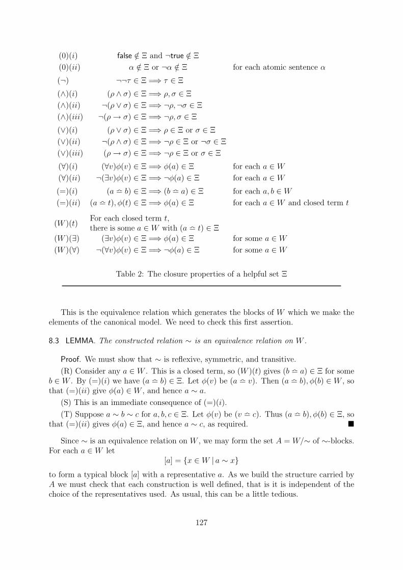
(0)(i) false /∈ Ξ and ¬true /∈ Ξ

(0)(ii) α /∈ Ξ or ¬α /∈ Ξ for each atomic sentence α

(¬) ¬¬τ ∈ Ξ =⇒ τ ∈ Ξ

(∧)(i) (ρ ∧ σ) ∈ Ξ =⇒ ρ, σ ∈ Ξ

(∧)(ii) ¬(ρ ∨ σ) ∈ Ξ =⇒ ¬ρ,¬σ ∈ Ξ

(∧)(iii) ¬(ρ→ σ) ∈ Ξ =⇒ ¬ρ, σ ∈ Ξ

(∨)(i) (ρ ∨ σ) ∈ Ξ =⇒ ρ ∈ Ξ or σ ∈ Ξ

(∨)(ii) ¬(ρ ∧ σ) ∈ Ξ =⇒ ¬ρ ∈ Ξ or ¬σ ∈ Ξ

(∨)(iii) (ρ→ σ) ∈ Ξ =⇒ ¬ρ ∈ Ξ or σ ∈ Ξ

(∀)(i) (∀v)φ(v) ∈ Ξ =⇒ φ(a) ∈ Ξ for each a ∈ W(∀)(ii) ¬(∃v)φ(v) ∈ Ξ =⇒ ¬φ(a) ∈ Ξ for each a ∈ W(=)(i) (a l b) ∈ Ξ =⇒ (b l a) ∈ Ξ for each a, b ∈ W(=)(ii) (a l t), φ(t) ∈ Ξ =⇒ φ(a) ∈ Ξ for each a ∈ W and closed term t

(W )(t)For each closed term t,there is some a ∈ W with (a l t) ∈ Ξ

(W )(∃) (∃v)φ(v) ∈ Ξ =⇒ φ(a) ∈ Ξ for some a ∈ W(W )(∀) ¬(∀v)φ(v) ∈ Ξ =⇒ ¬φ(a) ∈ Ξ for some a ∈ W

Table 2: The closure properties of a helpful set Ξ

This is the equivalence relation which generates the blocks of W which we make theelements of the canonical model. We need to check this first assertion.

8.3 LEMMA. The constructed relation ∼ is an equivalence relation on W .

Proof. We must show that ∼ is reflexive, symmetric, and transitive.

(R) Consider any a ∈ W . This is a closed term, so (W )(t) gives (b l a) ∈ Ξ for someb ∈ W . By (=)(i) we have (a l b) ∈ Ξ. Let φ(v) be (a l v). Then (a l b), φ(b) ∈ W , sothat (=)(ii) give φ(a) ∈ W , and hence a ∼ a.

(S) This is an immediate consequence of (=)(i).

(T) Suppose a ∼ b ∼ c for a, b, c ∈ Ξ. Let φ(v) be (v l c). Thus (a l b), φ(b) ∈ Ξ, sothat (=)(ii) gives φ(a) ∈ Ξ, and hence a ∼ c, as required.

Since ∼ is an equivalence relation on W , we may form the set A = W/∼ of ∼-blocks.For each a ∈ W let

[a] = x ∈ W | a ∼ x

to form a typical block [a] with a representative a. As we build the structure carried byA we must check that each construction is well defined, that is it is independent of thechoice of the representatives used. As usual, this can be a little tedious.

127

To produce a structure carried by A we must construct interpretations for each symbolof the signature of L(W ). Thus we require attributes

[[K]] [[R]] [[O]] [[a]]

for each constant symbol, each relation symbol, and each operation symbol O of L, andeach a ∈ W . Clearly, we take

[[a]] = [a]

for each a ∈ W . The other attributes take just a little longer to produce.As we go through the construction we will need several facts concerning the interaction

of ∼ and the set Ξ. Here is the first of these.

8.4 LEMMA. Suppose (a l t) ∈ Ξ for some a ∈ W and closed term t. Then

(b l t) ∈ Ξ ⇐⇒ a ∼ b

holds for each b ∈ W .

Proof. Suppose (b l t) ∈ Ξ. Let φ(v) be (b l t), so that (a l t), φ(t) ∈ ξ. Thus(=)(ii) give the required result.

Conversely, suppose a ∼ b. Let φ(v) be (v l t), so that (b l a), φ(a) ∈ Ξ. Thus(=)(ii) give the required result.

The constant symbol K is a close term. Thus, by (W )(t), we have

(a l K) ∈ Ξ

for at least on a ∈ W . There may be several such a. However, Lemma 8.4 gives

(b l K) ∈ Ξ ⇐⇒ a ∼ b

so we may take[[K]] = [a]

and use any b ∈ [a] as a name of [[K]].We use a similar method to produce [[R]] and [[O]]. But before we look at the details,

let’s obtain a useful generalization of (=)(ii).

8.5 LEMMA. Let φ(v1, . . . , vn) be a formula (of L(W )) with indicated free variables. Leta1, . . . , an ∈ W and let t1, . . . , tn be closed terms such that

(ai l ti) ∈ Ξ

for each 1 ≤ i ≤ n. Then

φ(t1, . . . , tn) ∈ Ξ =⇒ φ(a1, . . . , an) ∈ Ξ

holds.

128

Proof. For the time being fix i with 1 ≤ i ≤ n. let φi(v) be

φ(t1, . . . , ti−1, v, ti+1, . . . , tn)

where the free variable occurs in position i of φ and all the other free variables areinstantiated. Then (=)(ii) show that

(ai l ti), φ(ti) ∈ Ξ =⇒ φi(ai)

holds. We use this several times for different i and different selections of terms. Thus

φ(t1, t2, . . . , tn−1, tn) ∈ Ξ =⇒ φ(a1, t2, . . . , tn−1, tn) ∈ Ξ since (a1 l t1) ∈ Ξ

=⇒ φ(a1, a2, . . . , tn−1, tn) ∈ Ξ since (a2 l t2) ∈ Ξ...

=⇒ φ(a1, a2, . . . , an−1, tn) ∈ Ξ since . . .

=⇒ φ(a1, a2, . . . , an−1, an) ∈ Ξ since (an l tn) ∈ Ξ

to give the required result.

It’s time to produce [[R]] and [[O]].

Let R be a n-placed relation symbol of the signature of L. How do we produce then-placed relation [[R]] on A? We must determine when

[[R]][a1] · · · [an]

is true and when it is false for each [a1], . . . , [an] ∈ A.We wish to define [[R]] by

[[R]][a1] · · · [an] ⇐⇒ Ra1 · · · an ∈ Ξ

where a1, . . . , an are representative of the blocks involved. However, this definition willmake sense only if the equivalence is independent of the representatives.

Let b1, . . . , bn be a different set of representatives. Thus

ai ∼ bi

for each 1 ≤ i ≤ n. Using Lemma 8.5 we have

Ra1 · · · an ∈ Ξ ⇐⇒ Rb1 · · · bn ∈ Ξ

so that, as required, the attempted construction of [[R]] is well defined.

Let O be a n-placed operation symbol of the signature of L. How do we produce then-placed operation [[O]] on A? We must determine an output

[[O]][a1] · · · [an]

in A for each selection [a1], . . . , [an] of inputs in A.Let a1, . . . , an be representatives of the input blocks. Observe that

t = Oa1 · · · an

129

is a closed term of L(W ), and hence (W )(t) gives

(a l Oa1 · · · an) ∈ Ξ

for some a ∈ W . We wish to set

[[O]][a1] · · · [an] = [a]

but before we can do that, we must check that it makes sense.Let b1, . . . , bn ∈ W satisfy

ai ∼ bi

for each 1 ≤ i ≤ n. Thus we have a second set of representative for the input blocks. Let

(b l Ob1 · · · bn) ∈ Ξ

so that [b] is an attempted output for these representatives. A use of Lemma 8.5 gives

(b l Oa1 · · · an) ∈ Ξ

and then Lemma 8.4 gives a ∼ b so that, as required, the attempted construction of [[O]]is well defined.

This completes the construction of the structure M(Ξ). We now begin to relate itproperties to those of Ξ, and eventually we show that M(Ξ) is a model of Ξ. We workthrough several phases following the overall definition of the satisfaction relation givenin section 1.3.

Consider a closed term t of L(W ). This has some value [[t]] in A as generated byDefinition 1.13. Here, however, we do not need an assignment, (since each term we meetis closed). There is also a more direct way to determine [[t]].

8.6 LEMMA. The implication

(a l t) ∈ Ξ =⇒ [[t]] = [a]

holds for each closed term t and a ∈ W .

Proof. We proceed by induction on the construction of t.The base case, when t is a constant symbol K, is immediate from the definition of

[[K]].For the induction step, suppose

t = Ot1 · · · tn

whereO is an n-placed operation symbol and t1, . . . tn a smaller terms. For each 1 ≤ i ≤ n,(W )(t) gives some ai ∈ W with (ai l ti) ∈ Ξ, and then [[ti]] = [ai] follows by the inductionhypothesis. Consider any a ∈ W such that

(a l t) ∈ Ξ

holds. Lemma 8.5 gives(a l Oa1 · · · an) ∈ Ξ

130

and then Definition 1.13 gives the required

[[t]] = [[O]][[t1]] · · · [[tn]] = [[O]][a1] · · · [an] = [a]

where the last step holds by the definition of [[O]].

This is most of the finicky work done. To show that M(Ξ) is a model of Ξ we showthat

τ ∈ Ξ =⇒ M(Ξ) |= τ

holds for each sentence τ . Of course, we proceed by induction on the construction of τ .

8.7 LEMMA. For each atomic sentence τ both

τ ∈ Ξ =⇒ M(Ξ) |= τ ¬τ ∈ Ξ =⇒ M(Ξ) |= ¬τ

hold.

Proof. Each atomic sentence has one of the forms

true false (s l t) Rt1 · · · tn

where s, t, t1, . . . , tn are closed terms and R is a n-placed relation symbol. Let’s look atthe case where τ has the fourth form.

By (W )(t) there are ai ∈ W such that

(ai l ti) ∈ Ξ

for each 1 ≤ i ≤ n, and then[[ti]] = [ai]

by Lemma 1.6. Thus

M(Ξ) |= τ ⇐⇒ [[R]][[t1]] · · · [[tn]] ⇐⇒ [[R]][a1] · · · [an] ⇐⇒ Ra1 · · · an ∈ Ξ

using Definition 1.16 and the definition of [[R]]. With this Lemma 8.5 gives

τ ∈ Ξ =⇒ Ra1 · · · an ∈ Ξ =⇒ A |= τ

and a similar argument using (0)(ii) gives

¬τ ∈ Ξ =⇒ ¬(Ra1 · · · an) ∈ Ξ =⇒ Ra1 · · · an /∈ Ξ =⇒ not(M(Ξ) |= τ) =⇒ M(Ξ) |= ¬τ

as required.

So far we haven’t used any of the conditions (¬) — (∀)(ii), and neither (W )(∃) nor(W )(∀) These merely unravel the semantics of M(Ξ) and lead to a proof of the following.

8.8 THEOREM. The implication

τ ∈ Ξ =⇒ M(Ξ) |= τ

holds for each sentence τ . In particular, M(Ξ) is a model of Ξ.

Naturally, we call M(Ξ) the canonical model of Ξ.

131

Exercises

8.1 Complete the proof of Theorem 8.8.

[Held in 120-../C17-bit.. Last changed July 26, 2004]

8.2 Consistency property

By Theorem 8.8, to show that a set Σ of L(W )-sentences has a model, it is sufficientto embed Σ in a helpful set Ξ. We do this by maximizing in a certain way. The con-ditions (0)(i) — (=)(ii) are fairly easy to arrange, but the three witnessing conditions(W )(t), (W )(∃), (W )(∀) are more delicate. We need a mechanism to help guide the max-imizing process.

We work with certain families Con of sets Σ of L(W )-sentences. These families musthave certain closure properties.

8.9 DEFINITION. Let Con be a family of sets L(W )-sentences.Con is downward closed if

Γ ⊆ Σ ∈ Con =⇒ Γ ∈ Con

holds.Con has finite character if Σ ∈ Con whenever Γ ∈ Con for each finite Γ ⊆ Σ.

The finite character ensures that a consistency property Con is closed under union ofchains (and directed families), and so Zorn’s Lemma gives us maximal members of Con .Unfortunately, this process is too crude to give us what we need.

8.10 DEFINITION. A consistency property is a family Con of sets of L(W )-sentenceswhich is downward closed, has finite character, and for each Σ ∈ Con the conditions ofTable 3 hold.

There are several examples of consistency properties. The one we need (for the com-pactness theorem) is based on finite satisfiability.

8.11 THEOREM. The family FinSat of finitely satisfiable sets of L(W )-sentences is aconsistency property.

Proof. Almost trivially, FinSat is downward closed and has finite character. It isroutine to check that FinSat has properties (0)(i) — (=)(ii), for these just unravel thesemantics of sentences. The three witnessing conditions (W )(t), (W (∃), and (W )(∀) arenot so immediate.

Consider any Σ ∈ FinSat and look at

Σ ∪ (a l t)

where t is a closed term and a is a witness that does not appear in Σ not in t. Any finitesubset of this set is a subset of

Γ ∪ (a l t)

132

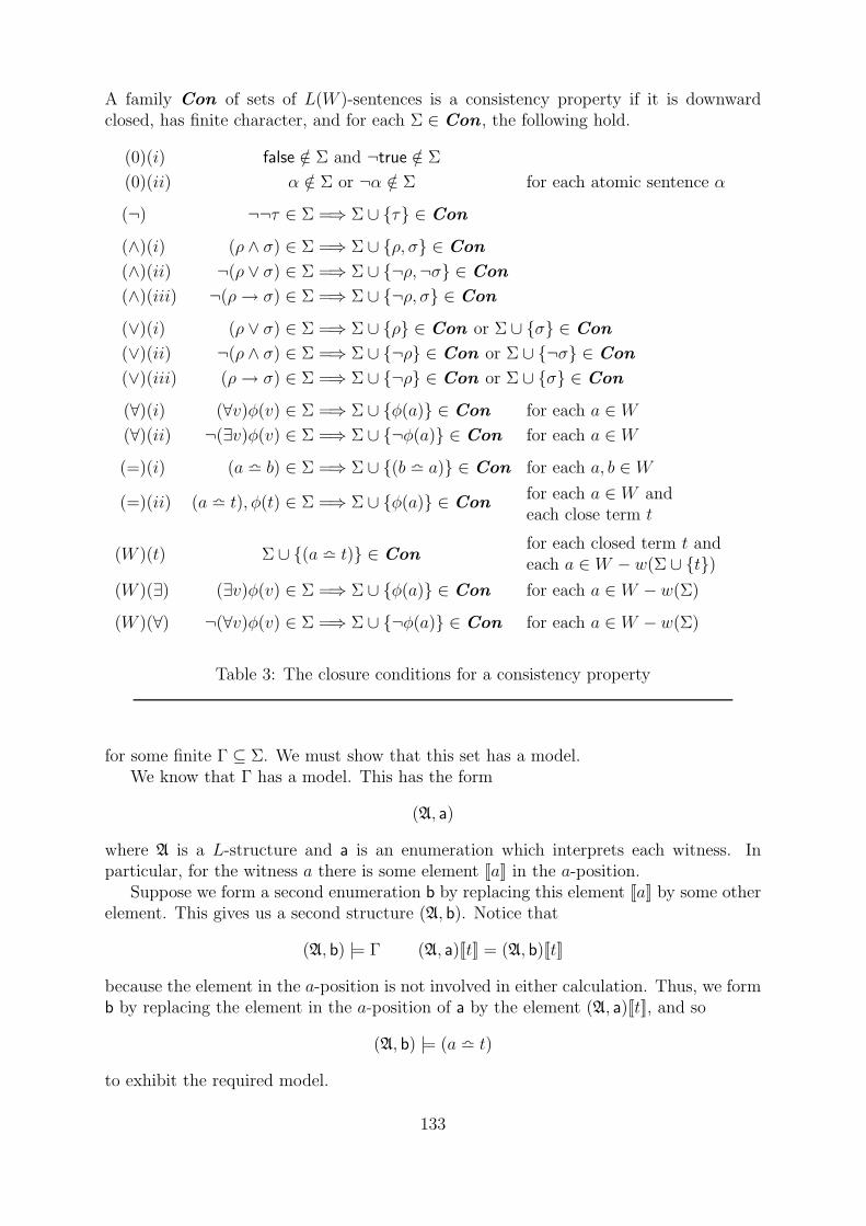
A family Con of sets of L(W )-sentences is a consistency property if it is downwardclosed, has finite character, and for each Σ ∈ Con , the following hold.

(0)(i) false /∈ Σ and ¬true /∈ Σ

(0)(ii) α /∈ Σ or ¬α /∈ Σ for each atomic sentence α

(¬) ¬¬τ ∈ Σ =⇒ Σ ∪ τ ∈ Con

(∧)(i) (ρ ∧ σ) ∈ Σ =⇒ Σ ∪ ρ, σ ∈ Con

(∧)(ii) ¬(ρ ∨ σ) ∈ Σ =⇒ Σ ∪ ¬ρ,¬σ ∈ Con

(∧)(iii) ¬(ρ→ σ) ∈ Σ =⇒ Σ ∪ ¬ρ, σ ∈ Con

(∨)(i) (ρ ∨ σ) ∈ Σ =⇒ Σ ∪ ρ ∈ Con or Σ ∪ σ ∈ Con

(∨)(ii) ¬(ρ ∧ σ) ∈ Σ =⇒ Σ ∪ ¬ρ ∈ Con or Σ ∪ ¬σ ∈ Con

(∨)(iii) (ρ→ σ) ∈ Σ =⇒ Σ ∪ ¬ρ ∈ Con or Σ ∪ σ ∈ Con

(∀)(i) (∀v)φ(v) ∈ Σ =⇒ Σ ∪ φ(a) ∈ Con for each a ∈ W(∀)(ii) ¬(∃v)φ(v) ∈ Σ =⇒ Σ ∪ ¬φ(a) ∈ Con for each a ∈ W

(=)(i) (a l b) ∈ Σ =⇒ Σ ∪ (b l a) ∈ Con for each a, b ∈ W

(=)(ii) (a l t), φ(t) ∈ Σ =⇒ Σ ∪ φ(a) ∈ Confor each a ∈ W andeach close term t

(W )(t) Σ ∪ (a l t) ∈ Confor each closed term t andeach a ∈ W − w(Σ ∪ t)

(W )(∃) (∃v)φ(v) ∈ Σ =⇒ Σ ∪ φ(a) ∈ Con for each a ∈ W − w(Σ)

(W )(∀) ¬(∀v)φ(v) ∈ Σ =⇒ Σ ∪ ¬φ(a) ∈ Con for each a ∈ W − w(Σ)

Table 3: The closure conditions for a consistency property

for some finite Γ ⊆ Σ. We must show that this set has a model.We know that Γ has a model. This has the form

(A, a)

where A is a L-structure and a is an enumeration which interprets each witness. Inparticular, for the witness a there is some element [[a]] in the a-position.

Suppose we form a second enumeration b by replacing this element [[a]] by some otherelement. This gives us a second structure (A, b). Notice that

(A, b) |= Γ (A, a)[[t]] = (A, b)[[t]]

because the element in the a-position is not involved in either calculation. Thus, we formb by replacing the element in the a-position of a by the element (A, a)[[t]], and so

(A, b) |= (a l t)

to exhibit the required model.

133

The same trick can be used to verify (W )(∃) and (W )(∀).For instance, consider any (∃v)φ(v) ∈ Σ ∈ Con and any witness a not occurring in

Σ. Any finite subset ofΣ ∪ φ(a)

is a subset ofΓ ∪ φ(a)

for some finite Γ ⊆ Σ with (∃v)φ(v) ∈ Γ. We know that Γ has a model (A, a), and wemodify this to obtain a model (A, b) of φ(a). We do this by altering the element in thea-position of a. Since (A, a) |= (∃v)φ(v) there is some element b with (A, a) |= φ(b). Weform b by putting b into the a-position, so that (A, b)[[a]] = b. This ensures that (A, b) isa model of Γ ∪ φ(a), as required.

You should compare Table 3 with Table 2. Notice how that conditions in the twotables match. In particular, conditions (0)(i) — (=)ii) of Table 3 ensure that eachmaximal member of Con will satifies the conditions (0)(i) — (=)ii) of Table 2. Butthe witnessing conditions are different. The conditions Table 3 give us enough room tomanipulate the witnesses into the places we want them, provided we start from a positionwith enough room.

For each set Σ of L(W )-sentences, let w(Σ) be the set of witnesses occurring in W .Thus w(Σ) ⊆ W and could be the whole of W . However, we want to make sure there isenough witesses left in W − w(Σ) to do any job that might turn up. The easiest way toachieve this is to impose a cardinality condition in w(Σ).

8.12 THEOREM. Let κ = |L| = |W | = |L(W )|.Let Con be a consistency property.Let Σ ∈ Con and suppose ν = |w(Σ)| < κ.Then Σ ⊆ Ξ ∈ Con for some helpful set Ξ.

Proof. We obtain Ξ by a maximizing argument. A simple use of Zorn’s Lemmawill achieve (0)(i) — (=)(ii) of Table 2, but may not achieve the witnessing conditions(W )(t), (W )(∃), and (W )(∀). To do that we move from Σ to Ξ in a more controlled way.The initial condition ν < κ gives us enough room to organize the witnesses to do the jobsrequired.

Let(τi | i < κ) (ti |, i < κ)

be ordinal indexed families of all L(W )-sentences τ and all closed L(W )-terms t. Thereare no restrictions on these enumerations, and can contain repetitions.

We produce an ascending chain

(Σ) Σ = Σ0 ⊆ · · · ⊆ Σi ⊆ · · · (i < κ)

of members of Con withνi = |w(Σi)| ≤ maxν, |i|

for each i < κ. This condition will give us plenty of room to manoeuvre the witnesses atlater stages.

We setΣ0 = Σ Σ` =

⋃Σi | i < `

134

for each limit ordinal ` < κ. Note that

ν` = |w(Σ`)| = supνi |, i < ` ≤ maxν, |`| < κ

to preserve the cardinality condition.At the step Σi 7→ Σi+1 we deal with the sentence τ = τi and the term t = ti. We

produce two intermediate stages

Σi ⊆ Σ′i ⊆ Σ′′

i ⊆ Σi+1

each designed to do a particular job. At each stage we use no more than finitely manynew witnesses, so that νi+1 = νi+n for some n ∈ N. This ensure the cardinality conditionis preserved.

We know that Σi ∈ Con .For the first stage we look at τ = τi and set

Σ′i =

Σi ∪ τ if this is in ConΣi otherwise

so that Σ′i ∈ Con and the cardinality restriction is preserved.

We now inspect the shape of τ . If τ is of neither of the shapes

(∃v)φ(v) ¬(∀v)φ(v)

then we set Σ′′i = Σ′

i and proceed to the next stage. It τ is of one of these shapes, Thenwe arrange that (W )(∃) or (W )(∀) of Table 2 holds. We have |w(Σ′

i)| < κ = |W | so wemay select a new witness a ∈ W − w(Σ′

i), and set

Σ′′i = Σ′

i ∪ φ(a) Σ′′i = Σ′

i ∪ ¬φ(a)

accordingly. The corresponding consistency property (W )(∃) or (W )(∀) of Table 3 ensuresthat Σ′′

i ∈ Con , and, of course, the cardinality restriction is preserved.Finally, we deal with the closed term t = ti. We have |w(Σ′′

i ∪ t)| < κ = |W | so wemay select a new witness a ∈ W − w(Σ′′

i ∪ t), and set

Σi+1 = Σ′′i ∪ (a l t)

to complete this step. Notice that the consistency property (W )(t) of of Table 3 ensuresthat Σi+1 ∈ Con .

Consider the chain Σ generated in this way. We set

Ξ =⋃

Σ

so that Ξ ∈ Con . We need to check that Ξ has the closure properties of Table 2.Each of the conditions (0)(i) — (=)(ii) follows from the corresponding consistency

property of Table 3. Let’s look at a few of these verifications.

(∧)(i) Suppose ρ ∧ σ ∈ Ξ for some sentences ρ, σ. Note that ρ ∧ σ ∈ Σi for allsufficiently large i, and hence the closure condition (∧)(i) (of Table 3) gives

Σi ∪ ρ, σ ∈ Con

135

for all such i. Let ρ = τr and σ = τs to locate two particular indexes r, s < κ. We havearranged that

Σr ∪ ρ ∈ Con =⇒ ρ ∈ Σr+1 ⊆ Ξ Σs ∪ σ ∈ Con =⇒ σ ∈ Σs+1 ⊆ Ξ

hold. Now consider any sufficiently large i > r, s. Then

Σr ∪ Σs ∪ ρ, σ ⊆ Σi ∪ ρ, σ ∈ Con

so thatΣr ∪ ρ ∈ Con Σsr ∪ σ ∈ Con

and hence ρ, σ ∈ Ξ, as required.

(∨)(i) Suppose ρ ∨ σ ∈ Ξ for some sentences ρ, σ. Note that ρ ∨ σ ∈ Σi for allsufficiently large i, and hence the closure condition (∨)(i) (of Table 3) ensures that oneof

Σi ∪ ρ ∈ Con Σi ∪ σ ∈ Con

holds for all such i. Let ρ = τr and σ = τs to locate two particular indexes r, s < κ. Wehave arranged that

Σr ∪ ρ ∈ Con =⇒ ρ ∈ Σr+1 ⊆ Ξ Σs ∪ σ ∈ Con =⇒ σ ∈ Σs+1 ⊆ Ξ

hold. Now consider any sufficiently large i > r, s. Then one of

Σr ∪ ρ ⊆ Σi ∪ ρ ∈ Con Σs ∪ σ ⊆ Σi ∪ σ ∈ Con

holds, so that one of

Σr ∪ ρ ∈ Con Σs ∪ σ ∈ Con

holds, and hence we have one of

ρ ∈ Ξ σ ∈ Ξ

as required.

Each of the conditions (0)(i) — (=)(ii) follows by a similar kind or argument. Let’slook at the final last one.

(=)(ii) Suppose (a l t), φ(t) ∈ Ξ for some a ∈ W , some closed term t, and someformula φ(v). Note that

(a l t), φ(t) ∈ Σi

for all sufficiently large i. and hence the closure condition (=)(ii) (of Table 3) ensuresthat

Σi ∪ φ(a) ∈ Con

holds for all such i. Let φ(a) = τr to locate a particular index. Consider any sufficientlylarge i > r. We have

Σr ∪ φ(a) ⊆ Σi ∪ φ(a) ∈ Con

so thatΣr ∪ φ(a) ∈ Con

136

and hence, by the construction, we have

φ(a) ∈ Σr+1 ⊆ Ξ

as required.

It remains to verify the witnessing conditions (W )(t), (W )(∃), and (W )(∀). Thearguments for these are similar to the above arguments, but let;s look at two of them.

(W )(t) Consider any close term t, and let t = ti to locate an index i < κ. At the stepi 7→ i+ 1 we have arranged that

(a l t) ∈ Σi+1 ⊆ Ξ

for some a ∈ W , as required.

(W )(∃). Consider any sentence τ = (∃v)φ(v) ∈ Ξ. Let τ = τi to locate an indexi < κ. Since Σi ∪ τ ⊆ Ξ, we have Σi ∪ τ ∈ Con , and hence we have arranged that

τ ∈ Σ′i φ(a) ∈ Σ′′

i ⊆ Ξ

for some a ∈ W , as required.

This completes the whole proof.

How does this prove the refined compactness theorem for a language L? Consider anyset Σ is L-sentences which is finitely satisfiable. We may view Σ as a set of L(W )-sentenceswith w(Σ) = ∅. As such we have Σ ∈ FinSat where this is the consistency property ofTheorem 8.11. Furthermore, there are no witnesses in Σ, so that |w(Σ)| = 0 < |L|, andhence Theorem 8.12 gives Σ ⊆ Ξ ∈ FinSat for some helpful set Ξ. By Theorem 8.8, Ξhas a canonical model and this, of course, provides a model of Σ. The construction ofthis structure ensures that it has cardinality no bigger than |W | = |L|.

The compleness theorem can be proved in the same way. We use

Σ ∈ ProofCon ⇐⇒ not(Σ ˙ false)

to produce from a formal proof system ˙ a family ProofCon of sets Σ of L(W )-sentences. The formal proof rules are designed to ensure that ProofCon is a consistenceyproperty. A simple argument then gives the adequacy of the system.

Exercises

8.2 Complete the proof of Theorem 8.12

8.3 Use the notion of a consistency property to design a system of formal proofs whichis complete.

137


9 Omitting types

Consider any set Γ of formulas (in some language L). For each φ ∈ Γ the set ∂φ is finite,but the set

∂Γ =⋃∂φ |φ ∈ Γ

may be infinite (for different formulas may use different variables).

9.1 DEFINITION. let L be a language.(a) A type (in L) is a set Γ of formulas such that ∂Γ is finite. Sometimes we write

Γ(v) to indicate that ∂Γ = v.(b) A type Γ is realized in a structure A (suitable for L) if A |= Γ(a) for some point

a of A (matching the free variables of Γ).(c) A type is omitted in a structure if it is not realized in that structure.

Compactness arguments can be used to produce a structure which realizes a giventype, but how can we produce a structure which omits a type? We have seen alreadyan example of such a construction. By Theorem 5.29, a submodel A of a theory T is inE(T ) if an only if A omits a certain family of types. However, the construction of A, as inLemma 5.31 and Theorem 5.32, is rather crude, and doesn’t refine in a straight forwardmanner. In general, to omit types we need some restrictions on the situation.

9.2 DEFINITION. Let T be a theory.(ω) Let Γ be a type. The type Γ is principal over T if there is a formula θ (with

∂θ = ∂Γ) which is consistent with T and such that

T ` θ →∧

Γ

holds.(0) Let Π be a ∀1-type, that is type of ∀1-formulas. The type Π is ∃1-principal over T

if there is an ∃1-formula θ (with ∂θ = ∂Π) which is consistent with T and such that

T ` θ →∧

Π

holds.

In the 0-version we put a restriction on the quantifier complexity of both the typeand the generating formula. If this generating formula is realized in any model of thetheory, then we automatically realize the type. However, that does not help us to omitthe type. In fact, to ensure that a type can be omitted it should not be principal.

9.3 EXAMPLE. Let T be a theory. Recall that for each ∀1-formula φ we set

Ω(T, φ) = φ ∪ ¬∃1(T, φ)

where ∃1(T, φ) is the set of ∃1-formulas θ such that

T ∪ θ is consistent T ` θ → φ

hold. Thus Ω(T, φ) is an ∀1-type. Almost by construction, this type is not ∃1-principalover T (for think what an ∃1-generator could be).

139

The proof of the following result is rather involved. However, the technique used isimportant, so we will take it rather slowly.

9.4 THEOREM. Let T be a theory in a countable language L. Let Π be countablecollection of ∀1-types each of which is not ∃1-principal over T . Then there is a countablestructure A ∈ S(T ) which omits each type in Π.

Proof. We enrich the language L to a language L(a) be adding countably manyparameters a. We will produce a structure (A, a) for L(a) such that a enumerates thewhole of A, and this is the required structure.

To obtain (A, a) we first produce a set Ξ of ∃1-sentence of L(a) such that the followinghold.

(i) T ∪ Ξ is consistent.

(ii) For each ∃1-sentence τ of L(a), if T ∪ Ξ ∪ τ is consistent then τ ∈ Ξ.

(iii) For each quantifier-free formula δ(v) of L(a), if (∃v)δ(v) ∈ Ξ then δ(a) ∈ Ξ for someselection a of parameters (matching v).

(iv) For each Π(v) ∈ Π and selection a of parameters (matching v), there is someformula φ(v) ∈ Π(v) with ¬φ(a) ∈ Ξ.

Suppose we have found such a set Ξ. By (i) there is a model (B, a) of T ∪ Ξ. Let A

be the substructure of B generated by a. Thus (A, a) ⊆ (B, a). As yet, we do not knowthat a enumerates the whole of A, but we will prove this shortly.

Consider any τ ∈ Ξ. Thenτ = (∃v)δ(v)

for some quantifier-free formula δ(v) of L(a). This δ may contain parameters not shownexplicitly. By (iii) we have δ(a) ∈ Ξ for some selection a of parameters. This gives(B, a) |= δ(a), and hence (A, a) |= δ(a), so that (A, a) |= τ .

Using this argument we draw a couple of conclusions.Firstly it shows that (A, a) |= Ξ.Now consider any ∃1-sentence τ of L(a) where (B, a) |= τ . Then T ∪ Ξ ∪ τ is

consistent, so that (ii) gives τ ∈ Ξ, and hence (A, a) |= τ . This shows that

B |= θ(a) =⇒ A |= θ(a)

for each ∃1-formula θ(v) of L and each point a from a.Next we see that a enumerates the whole of A. For consider a sentence

τ := (∃v)[v = Oa1, . . . , an]

where O is an n-placed operation symbol and a1, . . . , an are parameters. This ∃1-sentenceof L(a) is true in B, and hence τ ∈ Ξ (as in the previous paragraph). But now (iii) givesome elemement a ∈ a with

(a = Oa1, . . . , an) ∈ Ξ

to show that a is closed under O.

140

From this, we see that(A, a) ≺1 (B, a)

holds.Finally, consider any type Π(v) ∈ Π and any selection a of parameters matching v.

By (iv) we have ¬φ(a) ∈ Ξ for some φ(v) ∈ Π(v). But now A |= φ(a), and hence A doesnot realize Π(v) at a. Since a enumerates the whole of A, this shows that A omits Π(v).

Our job now is to produce such a set Ξ of sentence of L(a). This is where the assumedcountability is important.

Consider a triple(τ,Π(v), a)

where τ is an ∃1-sentence of L(a), where Π(v) ∈ Π, and where a is a selection of param-eters matching v. The language L(a) is countable, and the collection Π is countable, sothere are just countably many such triples. Let

(τ,Π(v), a)i i < ω

be an enumeration of all such triples.We produce Ξ as the union of an ascending chain

Ξ0 ⊆ Ξ1 ⊆ · · · ⊆ Ξi ⊆ . . . i < ω

of finite sets of ∃1-sentences of L(a). We generate this ω-chain by recursion on i. Weensure that each T∪Ξi is consistent, so that (i) will hold. The other requirements (ii,iii,iv)are dealt with during the course of the construction. The step Ξi 7→ Ξi+1 deals with thetriple (τ,Π(v), a) with index i.

At the base we set Ξ0 = ∅.Suppose we have obtain the finite set Ξi which is consistent with T . We look at the

i-triple(τ,Π(v), a)

enumerated above. Using this we do several things to obtain Ξi+1.

(v) If T ∪ Ξi ∪ τ is consistent we put

Ξ′i = Ξi ∪ τ

otherwise we put Ξ′i = Ξi.

(vi) We have a finite set Ξ′i of ∃1-sentences of L(a) which is consistent with T . Since

Π(v) is not ∃1-principal over T we know that

T ∪ Ξ′i `

∧Π(a)

can not hold. (If it does hold, then∧

Ξ′i will produce a generator of Π(v) over T .)

Thus there is some φ(v) ∈ Π(v) such that

T ∪ Ξ′i ∪ ¬φ(a)

is consistent. We putΞ′′

i = Ξ′i ∪ ¬φ(a)

to obtain a further extension of Ξ′i.

141

(vii) To get from Ξi to Ξ′′i we may have put in one or two new ∃1-sentence of L(a). Each

of these has the form(∃v)δ(v)

where δ(v) is a quantifier-free formula of L(a) (where the occurring parameters havenot been displayed). In total there are only finitely many parameters occurring inΞ′′

i , so there are plenty that have not yet been used. We may select a point a of newparameters matching v (the free variables of this δ). With this, T ∪ Ξ′′

i ∪ δ(a) isconsistent. We witness all the new ∃1-sentences in the same way to obtain Ξi+1.

Once this construction has be carried out we set

Ξ =⋃Ξi | i < ω

to obtain the final set Ξ.

Why does this set Ξ satisfy (i,ii,iii,iv)?

Property (i) holds since at each stage T ∪ Ξi is consistent.Property (ii) holds since this sentence τ is consider at some stage i. If T ∪ Ξ ∪ τ is

consistent, then so is T ∪ Ξi ∪ τ, and then (v) ensures that τ ∈ Ξi+1 ⊆ Ξ.Property (iii) holds by the final part of the step Ξi 7→ Ξi+1 described in (vii).Property (iv) holds by the arrangement described in (vi). The type Π(v) and the

selection a is part of a triple (τ,Π(v), a) considered at some stage i. The small stepΞ′

i 7→ Ξ′′i ensures that ¬φ(a) ∈ Ξi+1 ⊆ Ξ for some φ(v) ∈ Ξ.

With this the proof is completed.

This result is the 0-version of the omitting types result. There is an analogous, andmore common, ω-version.

9.5 THEOREM. Let T be a theory in a countable language L. Let Π be countable collec-tion of types each of which is not principal over T . Then there is a countable model A ofT which omits each type in Π.

This is proved by almost the same proof as Theorem 9.4. The difference is there is noquantifier complexity on the set Ξ is sentences of the enriched language L(a). From thiswe obtain a model (B, a) of T∪Ξ, and a generated substructure (A, a) of (B, a). However,we have to show that A ≺ B. Conditions (i, ii, ii, iv) and the generating conditions (v,vi, vii) are modified by removing all the restrictions on quantifier complexity.

Exercises

9.1 Theorem 9.4 can be strengthened. Prove the following.Let T be a theory in a countable language L. Let Π be countable collection of ∀1-types

each of which is not ∃1-principal over T . Then there s a countable structure A ∈ E(T )which omits each type in Π.

In other words, show that we can arrange that the omitting structure is e. c.


142

[Held in 120-../C30-bit.. Last changed July 26, 2004]

10 The back and forth technique

Recall that, from section 2.3, a line is a dense linear ordering without end points. Therationals Q and the reals R are the two best known examples of lines. However, since theclass of lines is elementary and its theory is ∀2-axiomatizable (if fact, it has EQ), we seethere are examples of lines in every (non-finite) cardinality. How can we compare thesedifferent lines.

Consider any two lines A and B , and let’s compare configurations in A with those inB. Thus, let

a = a1, . . . , an b = b1, . . . , bn

be, respectively, a point of A and a point of B. (Here, of course, we mean ‘point’ in thesense used throughout these notes, not in the sense of a geometrical point.) The elementsof a and b need not be listed in the order that they occur in their respective lines, butwe do want them to have the same configuration. Let us write

a ∼ b

to indicate this similarity. Thus, in detail, this means that

ai ≤ aj ⇐⇒ bi ≤ bj

holds for all i, j ∈ 1, . . . , n.Suppose now that we are given a new element x of A. We may attach x to the end

of a to form an extended point ax. This will have a certain configuration in A. Can wefind a element y of B such that

ax ∼ by

holds?We can, because both A and B are lines.If x = ai for some i, then we simply take y = bi. Thus we may suppose that x 6= ai

for each i. We divide the ai into two part, a left hand part L(A) and a right hand partR(A). Using x we let

ai ∈ L(A) ⇐⇒ ai < x ai < x⇐⇒ ai ∈ R(A)

to generate these part. Notice that

al < x < ar

holds for all al ∈ L(A) and ar ∈ R(A). We pass these parts across to B. Thus

bi ∈ L(B) ⇐⇒ ai ∈ L(A) ai ∈ R(A) ⇐⇒ bi ∈ R(B)

gives us two finite subsets L(B), R(B) of B. The similarity a ∼ b ensures that

bl < br

143

holds for all bl ∈ L(B), br ∈ R(B). Now we make the crucial observation. Because B isa line, there is some y ∈ B such that

bl < y < br

holds for all bl ∈ L(B) and br ∈ R(B). To see this simply consider the three possiblecases; L(B) = ∅, R(B) = ∅, both L(B) and R(B) non-empty. Remember that B has noleft hand end, has no right hand end, and is dense. This choice of y ensures that

ax ∼ by

holds.We want to extend this kind of argument to more general structures. To do that we

need a notion of ‘points in the same configuration’.

10.1 DEFINITION. Let A,B be structures for some language L. A partial isomorphismbetween A and B is a pair (a, b) of points (a from A and b from B) such that

(A, a) ≡0 (B, b)

holds.

For the case of lines a partial isomorphisms (a, b) is merely a pair of points in thesame configuration. The description of this used above sets down precisely what (A, a) ≡0

(B, b) means in this particlar case. In the same way we could set down the details ofwhat (A, a) ≡0 (B, b) means for the general case. We don’t do that because these detailsare never needed here. Notice that we do not assume that the points a and b enumeratesubstructures of A and B. However, the two points will generate substructures, and thesesubstructures will be canonically isomorphic.

10.2 DEFINITION. Let A,B be structures for some language L.(a) A back-and-forth system for the pair A,B is a non-empty set P of partial isomor-

phisms (a, b) with the following two properties.

(back) For each (a, b) ∈ P and each element y of B, there is an element x of A with(ax, by) ∈ P .

(forth) For each (a, b) ∈ P and each element x of A, there is an element y of B with(ax, by) ∈ P .

(b) We writeA ≡p B

and say A and B are potentially isomorphic if there is at least one back-and-forth systemfor the pair A,B.

For instance, we saw above that each pair of lines are potentially isomorphic. Inparticular, potential isomorphisms does not require that the two structures have thesame cardinality.

The relation ≡p should be compared with the semantic relations

≡n ≡ω

144

(for n < ω) and the isomorphism relation

≡∞

defined in section 3.1. We have used a similar notation for these relations because of thefollowing result.

10.3 THEOREM. For each pair A,B of structures (for some language), both the impli-cations

A ≡∞ B =⇒ A ≡p B =⇒ A ≡ω B

hold.

Proof. For the first implication suppose f is an isomorphism from A to B. Let P bethe set of finite restrictions of f . That is, P is the set of pair (a, b) where

a = a1, . . . , an b = b1 . . . , bn

and wherefai = bi

for each i ≤ i ≤ n. A simple calculation shows that this is a back-and-forth system.For the second implication suppose we have a back-and-forth system P for A,B. We

show that[n] (A, a) ≡n (B, n)

holds for each n < ω and each (a, b) ∈ P . We proceed by induction on n.The base case, [0] is trivial.For the induction step, [n] ⇒ [n+ 1], suppose

A |= (∃v1, . . . , vm)φ(vm, . . . , v1, a)

where (a, b) ∈ P and φ ∈ ∀n. There are elements x1, . . . , xm of A such that

A |= φ(xm, . . . , x1, a)

holds. By repeated use of the ‘forth’ property there are elements y1, . . . , ym of B suchthat

(ax1 · · ·xm, by1 · · · ym) ∈ Pholds, and hence

(A, ax1 · · ·xm) ≡n (B, by1 · · · ym)

by the induction hypothesis [n]. This gives

B |= φ(ym, . . . , y1, ba)

and henceB |= (∃v1, . . . , vm)φ(vm, . . . , v1, b)

holds.This, with a symmetric argument, gives [n+ 1].

As a simple consequence of this we see that the theory of lines is complete. Forany two lines A,B we have A ≡p B and hence A ≡ω B, in other words A and B areelementary equivalent.

Originally, back-and-forth systems were invented to generate full ismorphisms. Hereis that first use.

145

10.4 THEOREM. The implication

A ≡p B =⇒ A ≡∞ B

holds for all countable structures A,B.

Proof. Let P be a back-and-forth system for the two countable structures A and B.We use P to generate a full isomorphisms f from A to B.

Let A be the carrier of A and let B be the carrier of B. Since both A and B arecountable there are enumerations

xi yi i < ω

of these sets. (These enumerations can be quite arbitrary.) We use P to produce anascending chain

f0 ⊆ f1 ⊆ · · · ⊆ fi ⊆ i < ω

of partial isomorphismfi : Ai

- Bi

between finite subsets of A and B. Thus, for each i < ω we have

(A, a1, . . . , an) ≡0 (B, b0, . . . , bn)

wherea1, . . . , an

is an enumeration of Ai, and

b1 = fia1, . . . , bn = fian

is the corresponding enumeration of Bi. For each i < ω this constructed pair (a, b) ofenumerations will be in P and we will ensure that

xi ∈ Ai yi ∈ Bi

hold. The unionf =

⋃fi | i < ω

is then the required isomorphism.Suppose we have produced the partial isomorphism fi with (a, b) as the corresponding

pair. We look first at the element x = xi+1 of A. By the forth property there is someelement v of B with (ax, bv) ∈ P . We next look at the element y = yi+1 of B. By theback property there is some element u of A with (axu, bvy) ∈ P . We take this as theextension fi+1 of fi.

As a simple consquence of this we see that the theory of lines is ℵ0-categorical.

Homogeneous structures

Exercises

10.1 Show that potential isomorphism, ≡p, is an equivalence on the class of all structures(for a given language).

146

11 Homogeneous-universal models

147

12 Saturation – see earlier

148

13 Forcing techniques

149

14 Ultraproducts–to be done

150

Part III

Some solutions to the exercises

151

[Held in 120../B10-sols.. Last changed July 26, 2004]

A For section 1


A.1 For §1.1

1.1 The shape of the formulas can be seen by subscripting the different uses of thevariables in φ3.

φ3 := (∃u2)[(u2 < v3) ∧(∃v2)[(u2 l v2) ∧ φ2]] where

φ2 := (∃u1)[(u1 < v2) ∧(∃v1)[(u1 l v1) ∧ φ1]] where

φ1 := (∃u0)[(u0 < v1) ∧(∃v0)[(u0 l v0) ∧ φ0]] where

φ0 := (v0 l v0)

Continuing this sequence in the obvious way, a simple induction gives ∂φr = vr and∂θr = ur for each r < ω.

A.2 For §1.2–not yet done


A.3 For §1.3

1.4 (a) A simple induction shows that

N |= φr(a) ⇐⇒ r ≤ a

holds for each a ∈ N and r < ω.(b) This is an immediate consequence of (a).(c) Consider any such formula ψ(v). If there is any a ∈ N with N |= ψ(a) then, by

(a), we have r ≤ a for each r < ω. This is impossible, and hence there is no such a. ThusN |= ¬(∃v)ψ(v) must hold.


A.4 For §1.4 – most not done

1.13 (i)⇒(ii). Suppose T ∪σ is consistent and consider any A |= T ∪σ. Then, usingi, we have

B |= T =⇒ B ≡ A =⇒ B |= σ

153

so that σ ∈ T .(ii)⇒(iii). Suppose T ⊆ T ′ where T ′ is consistent. Then (ii) gives

σ ∈ T ′ =⇒ T ∪ σ consistent =⇒ σ ∈ T

and hence T = T ′.(iii)⇒(iv). We verify the contrapositive of (iv). Consider a pair of sentences σ, τ

neither of which is in T . Then both

T ∪ ¬σ T ∪ ¬τ

are consistent, and hence (iii) (or even (ii)) gives

T ` ¬σ T ` ¬τ

so that ¬σ ∧ ¬τ ∈ T , which leads to σ ∨ τ /∈ T .(iv)⇒(i). For each sentence σ, we have σ ∨ ¬σ ∈ T , and hence (iv) ensures that one

ofσ ∈ T ¬σ ∈ T

holds, which leads to the required result.

1.14 Let Ψ be the full binary splitting tree (sometimes called the Cantor tree). The nodesµ, ν, . . . of Ψ are the finite lists

i(0)i(1) · · · i(n− 1)

taken from 0, 1. This particular list has length n, and the empty list

⊥

of length 0 is allowed. These nodes are partially ordered by extension.

...000

...001

00

...010

...011

01

0

...100

...101

10

...110

...111

11

1

⊥

In particularν0 ν1

ν

is a typical node ν and its two successors ν0, ν1.We write

ν ≤ µ µ|ν

to indicate, respectively, that µ extends ν, and that µ and ν are incomparable.A branch of this tree is just a function

p : N - 0, 1

154

and there are 2ℵ0 such branches. This branch lies above the nodes

⊥, p(0), p(0)p(1), p(0)p(1)p(2), . . .

the finite initial sections of p.

Assuming that no finite extension of the theory T is complete, we produce a family

Σ = σν | ν ∈ Ψ⊥

of sentences, each consistent with T , with

σ⊥ = true

and such that

(i) ν ≤ µ =⇒ T ` σµ → σν (ii) µ|ν =⇒ T ` ¬σµ ∨ ¬σν

hold for all nodes µ, ν of Ψ.We generate this family by recursion up the tree Ψ. Suppose we have generated σν for

some ν ∈ Ψ. Thus T ∪ σν is consistent, and does not axiomatize a complete extensionof T . Thus there is a sentences τ such that both

T ∪ σν , τ T ∪ σν ,¬τ

are consistent. We setσν0 = σν ∧ τ σν1 = σν ∧ ¬τ

to produce the two immediate successors of σν . Note that

T ` σνi → σν T ` ¬σν0 ∨ ¬σν1

hold.Once we have the family Σ we set

Σp = σν | ν < p

for each branch p of Ψ. By (i) we see that each such theory T ∪ Σp is consistent. Let

Ap |= T ∪ Σp

to produce a complete extension T (p) = Th(Ap) of T . We show that these are pairwisedistinct.

Consider distinct branches p, q of Ψ. There are nodes µ < p, ν < q with µ|ν. Then(ii) gives

Ap |= ¬σν Aq |= ¬σµ

so that Aµ 6≡ Aq, as required.


155

A.5 For §1.5

1.16 (a) If Σ ` τ , then Σ ∪ ¬τ does not have a model, and hence, by compactness,some finite part of this set does not have a model. In other words, there is some finiteΓ ⊆ Σ such that Γ ∪ ¬τ does not have a model. With this Γ we have Γ ` τ , to givethe required result.

(b) Suppose Σ has the closure properties. We show that

Σ ` τ =⇒ τ ∈ Σ

holds, and hence Σ is a theory. (The other required implication is trivial.)Suppose Σ ` τ . By part (a) we have Γ ` τ for some finite part

Γ = σm, . . . , σ1

of Σ. But now the sentenceσm → · · ·σ1 → τ

is logically valid, and hence belongs to Σ. With this we may strip of σm, . . . , σ1 in turn,to get τ ∈ Σ.

1.17 Since each Kr is strictly elementary we have Kr = M(σr) for some family

Σ = σr | r < ω

of sentences. Since Kr ⊇ Kr+1 we may assume that ` σr+1 → σr holds. (This may beachieved by taking conjunctions of the original σr.)

We see that K = M(Σ), so that K is elementary.By way of contradiction, suppose that K is strictly elementary. Thus K = M(τ) for

some sentence τ . In particularΣ ` τ

and` τ → σr

for each r < ω. These give some particular n < ω such that ` τ ↔ σn, and henceK = M(σn) = Kn, which is not so.

1.18 LetK = M(σ) L = M(L) R = M(R)

where σ is a sentence and L,R are sets of sentences. Since L∩R = ∅, we see that L∪Rdoes not have a model, and hence compactness gives sentences λ, ρ such that

L ⊆M(λ ∧ σ) R ⊆M(ρ ∧ σ) ` ¬λ ∨ ¬ρ

hold. We show that, in fact,

L = M(λ ∧ σ) R = M(ρ ∧ σ)

hold.

156

Consider any A ∈ M(λ ∧ σ). Since A |= σ, we have A ∈ K = L ∪ R. Since A |= λ,we have A |= ¬ρ, and hence A /∈ R, to give A ∈ L, as required.

1.19 (a,b) Let α be conjunction of th eusual axioms for fields. This shows that F isstrictly elementary. and axiomatizes T .

For each prime p let

(p l 0) abbreviate 1 + · · ·+ 1 l 0

where there are p number of 1s in this sum. Then

α ∧ (p l 0)

axiomatizes Tp, to show that Fp is strictly elementary. Also

α ∪ (p 6l 0) | p a prime

axiomatizes T0, to show that F0 is elementary.We have

F0 ∪ Ff = F F0 ∩ Ff = ∅

so that, by Exercise 1.18, if Ff is elementary then F0 is strictly elementary. Part (c)show that this is not the case.

(c) For each τ ∈ T0 we have

T ∪ (p 6l 0) | p a prime ` τ

and henceT ∪ (2 6l 0), . . . , (p 6l 0) ` τ

for some sufficiently large prime p. Any field of larger prime characteristic show that thiscan not be so.

In particular, T0 is not finitely axiomatizable, and F0 is not strictly elementary.

(d) The same method show that

Tf ∪ (p 6l 0) | p a prime

is finitely satisfiable, and hence has a model.

1.20 For the first part all we need to observe is that Th(R) can be formalised in acountable language.

The second part depends on which signature is used.If we view R as a line (R,≤) (in the sense of subsection 2.3) then the rational line

(Q,≤) is the only possibility.If we view R in the most natural way as a linearly ordered real field, then the real

part of the algebraic closure of Q will do (and there are other possibilities).This second part requires some results not yet covered and some information about

the structure of real fields.

157


B For section 2


B.1 For §2.1

2.1 Since there are no operation symbols in the signature, each atomic sentence has oneof the shapes

true false (K1 l K2) RK1, · · ·Kn

where K1, . . . , Kn are constant symbols and R is an n-placed relation symbol. Since thesignature is finite, there are only finitely many such atomic sentences. Let α1, . . . , αn bethese atomic sentences.

Each quantifier-free sentence is T -equivalent to a conjunction of disjunction of literals.Each such disjunction can be put in the form

±α1 ∨ · · · ∨ ±αn

where each component ±α is α or ¬α, as approriate. There are only 2n possible dis-junctions of this kind. Each quantifier-free sentence is T -equivalent to a conjunction ofsuch disjunctions, and hence there are only finitely many quantifier-free sentences up toT -equivalence.

But every sentence is T -equivalent to a quantifier-free sentence, and hence the booleanalgebra of sentences modulo T is finite.

Each complete extension is determined by the set of sentences that need to be addedto T . Each such set is finite and, in fact, bounded by the size of the boolean algebra ofall sentences. Thus T has only finitely many complete extension.


B.2 For §2.2

2.2 We are required to show

(a) T+ ` (2) (b) T+ ` (3) (c) T ` (4)

where (4) is the sentence of Lemma 2.5.Handling internal (formal) induction can be quite tricky, especially when it is com-

bined with external induction.Let φ(v) be any formula with just the free variable v, as indicated. Notice that

(case) φ(0) ∧ (∀v)φ(Sv) .→. (∀v)φ(v)

is a simple consequence of the induction axiom for φ. This is the parameter-free caseinduction.

159

(a) Letφ(v) := (v l 0) ∨ (∃w)[Sw l v]

so thatT+ ` φ(0) T+ ` φ(Sv)

(for we can witness the approriate disjunct of φ). The required result

T+ ` (∀v)φ(v)

is an immediate application of (case).

(b) Letφk(v) := (Sk+1v 6l v)

(for each k ∈ N). First we check that

(i) T+ ` φ0(v) (ii) T+ ` φk+1(0) (iii) T+ ` φk(v) → φk+1(Sv)

hold.We have

T+ ` φ0(0)

by axiom (0), andT+ ` (S(Sv) l Sv) → (Sv l v)

by axiom (1), so thatT+ ` φ0(v) → φ0(Sv)

and hence a use of internal induction gives (i).An instance of axiom (0) fives (ii).By axiom (1) we have

T+ ` (Sk+2v l Sv) → (Sk+1v l v)

which gives (iii).We now show

[k] T+ ` (∀v)φk(v)

by an external induction over k.The base case [0], is just (i).For the induction step, [k] ⇒ [k + 1], we have

T+ ` (∀v)φk(v) → (∀v)φk+1(Sv)

by (iii), so that [k], (ii), and (case) give [k + 1].

(c) We prove the two implications of (4) separately.For each l ≤ k we have a sequence of implications

T ` (Sk+1w l v) ∧ (v l Sl0) → (Sk+1w l Sl0) → (S(k−l)+1w l 0) → false

by the properties of equality, axiom (2), and axiom (0). Thus

T ` (∃w)[Sk+1w l v) → (v 6l plq)

160

to giveT ` (∃w)[Sk+1w l v) → (v 6l p0q) ∧ · · · ∧ (v 6l pkq)

which is the first implication.For the converse let

φk(v) := (v l p0q) ∨ · · · ∨ (v l pkq) ∨ (∃w)[Sk+1w l v]

(for each k ∈ N). We first observe that

(iv) T ` φk+1(0) (v) T ` φk+1(Sv) ↔ φk(v)

hold. The first, (iv), is trivial. For the second, (v), we have

T ` φk+1(Sv) ↔ (Sv l p0q) ∨ (Sv l p1q) ∨ · · · ∨ (Sv l pk + 1q) ∨ (∃w)[Sk+2w l Sv]

↔ (Sv l p1q) ∨ · · · ∨ (Sv l pk + 1q) ∨ (∃w)[Sk+2w l Sv]↔ φk(v)

using first axiom (0), and then axiom (1). With these we show

[k] T ` (∀v)φk(v)

by an external induction over k.The base case [0], is axiom (2).For the induction step, [k] ⇒ [k + 1], we have

T ` (∀v)φk+1(Sv)

by [k] and (v), so that (iv) and (case) give [k + 1].

2.3 (a) Consider any element a of any model A of T . We may generate a chain

a(r) | r ∈ N

of elements of A by setting a(r) = Sra. By axiom (3) (as given in Solution 2.2), allthese elements are distinct. Thus we generate a copy of N. In particular, when a is thedistinguished element of A, we identify this copy with N. Recall that axiom (0) says that0 does not have a predecessor.

Now consider any element a not in (this canonical copy of) N. Using axiom (2) wemay regress to form a chain

a(−r) | r ∈ Nof elements of A where a(0) = a (as before) and Sa(−(r + 1)) = a(−r) for each r ∈ N.Using axiom (3) we see these two chains form a copy of Z = (Z, S, 0).

We now remove N from A. What we have left can be partitioned into blocks each ofwhich is a copy of Z. We count the number of such blocks, to see that

A = N ∪ Z(κ)

where the superscript indicates there are κ copies of Z. In particular, this κ completelydetermines the (ismorphism) type of A. Let us write A(κ) for this model. Thus everymodel is isomorphic to A(κ) for precisely one κ.

161

Notice that the cardinality of A(κ) is κ or ℵ0, which ever is the larger.

(b) For uncountable κ, each model of T of cardinality κ is isomorphic to A(κ).

(c) Each countable model of T is isomorphic to precisely one of

N = A(0) ⊆ A(1) ⊆ · · · ⊆ A(r) ⊆ · · · ⊆ A(ℵ0)

which is a chain of order type ω + 1.

This spectrum of models is typical of a large class of theories.[What are this kind of theories called?].

2.4 (a) Since N |= T , we haveT ` δ =⇒ N |= δ

(for each quantifier-free sentence), so it suffices to show that converse. There are twoways to do this.

Each atomic sentence α of this language has the shape

(pmq l pnq)

for some m,n ∈ N (or is one of true or false). Then

N |= α =⇒ (m = n) =⇒ T ` α

N |= ¬α =⇒ (m 6= n) =⇒ T ` ¬α

where the last implication makes use of axioms (1) and (0). Using this we show

N |= δ =⇒ T ` δ N |= ¬δ =⇒ T ` ¬δ

for each quantifier-free sentence δ. We proceed by induction on the construction of δ.Notice that we verify the two implications in tandem.

The base case, where δ is atomic, is just the observation above. For the inductionstep we survey the possible shapes of δ. There are four cases

δ = (α ∧ β) T ` ¬δ ↔ (¬α ∨ ¬β)δ = (α ∨ β) T ` ¬δ ↔ (¬α ∧ ¬β)δ = (α→ β) T ` ¬δ ↔ (α ∧ ¬β)δ = ¬γ T ` ¬δ ↔ γ

where α, β, γ are simpler sentences.For the first case we have

N |= δ =⇒ N |= α and N |= β =⇒ T ` α and T ` β =⇒ T ` δ

N |= ¬δ =⇒ N |= ¬α or N |= ¬β =⇒ T ` ¬α or T ` ¬β =⇒ T ` ¬δ

where, for both parts, the central implication uses the induction hypothesis.The second case is similar.For the third case we have

N |= δ =⇒ N |= ¬α or N |= β =⇒ T ` ¬α orT ` β =⇒ T ` δ

N |= ¬δ =⇒ N |= α and N |= ¬β =⇒ T ` α and T ` ¬β =⇒ T ` ¬δ

162

where again the central implications use the induction hypothesis.For the fourth case we have

N |= δ =⇒ N |= ¬γ =⇒ T ` ¬γ =⇒ T ` δ

N |= ¬δ =⇒ N |= γ =⇒ T ` γ =⇒ T ` ¬δ

where the central implications use the induction hypothesis. This is why we verify thetwo implications in tandem.

Another way to proveN |= δ =⇒ T ` δ

to to rephrase δ as a conjunction of disjunctions of literals, and then unravel this shape.

(b) We know that T ⊆ T+ ⊆ Th(N). For the converse, consider any sentence σ. Wehave

T ` σ ↔ δ

for some quantifier-free sentence δ. Then

N |= σ =⇒ N |= δ =⇒ T ` δ =⇒ T ` σ

using part (a), to give the required result.


B.3 For §2.3

2.6 Both Q and R are models of the theory T (of lines), which is complete, so thatTh(Q) = T = Th(R) and hence Q ≡ R.

This shows that the (Dedekind) completeness of the line R can not be captured in afirst order way (at least within the languages of lines).

2.7 Let (A,≤) be a linearly ordered set. We form a new linear ordering by replacingeach element of A by a copy of Q. These blocks are ordered as the occur in A. This givesthe ordinal product Q · A.

In more detail, we look at the set of pairs

(p, a)

where p ∈ Q and a ∈ A. We compare these by

(p, a) ≤ (q, b) ⇐⇒ (a < b) or [(a = b) and (p ≤ q)]

(for p, q ∈ Q and a, b ∈ A). It is routine to check that this gives a line, and a - (0, a)is an embedding.

2.8 The ℵ0-categoricity is the simplest application of the back-and-forth method. Thisis discussed in section 10.

Consider any cardinal κ > ℵ0. There are several methods of producing non-isomorphiclines of cardinality κ. Here is one of them.

163

Consider any limit ordinal λ of cardinality κ. Let λ∗ be the reverse of λ, and considerthe ordinal products

Q · λ Q · λ∗

both of which are lines of cardinality κ. We know that, as a linear order, λ is embeddedin the first, and λ∗ is embedded in the second. We show that λ∗ can not be embedded inthe first, and so the two are not isomorphic.

By way of contradiction suppose λ∗ can be embedded in Q · λ. Thus we have anindexed family

a(i) = (p(i), α(i)) (i < λ)

of elements of the line such that

j < i < λ =⇒ a(i) < a(j)

holds. Remembering how these pairs are compared, we see that

j < i < λ =⇒ α(i) ≤ α(j)

holds. In other words, we have a descending chain through λ. But λ is an ordinal, so thischain must stabilize after a finite number of steps. In other words, there is some finitek < ω such that

k ≤ j < i < λ =⇒ α(i) = α(j)

and hencek ≤ j < i < λ =⇒ p(i) < p(j)

holds. This gives a subset of Q of cardinality |λ| = κ, which is impossible.

B.4 For §2.4–not yet done

164


C For section 3


C.1 For §3.1

3.2 Suppose A ≺r B and A |= σ where σ is a ∃r+1-sentence. We have

σ = (∃v)φ(v)

for some ∀r-formula φ(v), and there is some point a of A with A |= φ(a). But now A ≺r B

gives B |= φ(a) so that B |= σ, as required.


C.2 For §3.2

3.3 Given such a pair of embeddings, for each ∀n+1-sentence we have

A |= σ =⇒ C |= σ =⇒ B |= σ

using first f then g.Conversely, suppose that A ≡〉(∀n+1) B holds. Let a be an enumeration of A and

let b be an enumeration of B. We enrich the underlying language L to both L(a) andL(b) and combine these to obtain L(a, b). We arrange that the a-parameters and theb-parameters are disjoint. Look at

Th(A, a) ∆(B, b) = Th(B, b) ∩ ∀n

which are, respectively, a set of L(a)-sentences and a set of L(b)-sentences. These combineto give

Th(A, a) ∪∆(B, b)

a set of L(a, b)-sentences, and it suffices to show that this set is consistent.By way of contradiction, suppose the set is not consistent. Then

Th(A, a) ` ¬δ(b)

for some ∀n-formular δ(w) and a point b of B with B |= δ(b). This gives first

Th(A, a) ` (∀w)¬δ(w)

and thenA |= (∀w)¬δ(w)

(since a and b are disjoint). But (∀w)¬δ(w) is a ∀n+1-sentence (of the original language),and hence

B |= (∀w)¬δ(w)

which leads to the contradiction.


165

C.3 For §3.3

3.5 This proof is very like that of Solution 3.3, and generalizes the proof of Lemma 3.19.On of the required implications is immediate. For the other suppose A ≺n+1 B. Let

a be an enumeration of A, and let b be an enumeration of B. It suffices to show that

Th(A, a) ∪ (Th(B, a, b) ∩ ∀n)

is consistent. The left hand component is a set of L(a) sentences. The right handcomponent is a set of L(a, b)-sentences, and will contains some sentences (a l b) wherea and b are parameters that name the same element of B.

By way of contradiction suppose the displayed set is not consistent. Then

Th(A, a) ` ¬δ(b, a)

for some ∀n-formula δ(v, u) of the parent language, an points a from a and b from b. Thisgives A |= (∀v)¬δ(v, a) and then B |= (∀v)¬δ(v, a) (since A ≺n+1 B), which leads to thecontradiction.


C.4 For §3.4

3.6 We verify this by induction on n.The base case, n = 0, is trivial.For the induction step, n 7→ n+ 1, suppose

A ⊆ B =⇒ A ≺n+1 B

for all A,B ∈ A. Consider any A ∈ A, and suppose

A |= (∀v)φ(v, a)

where φ(v, u) is a ∃n-formula, and a is a point from A. To show

U |= (∀v)φ(v, a)

consider any point b from U which matches v. There is some B ∈ A with A ⊆ B andsuch that b come from B. But now A ≺n+1 B, so that

B |= (∀v)φ(v, a)

and henceB |= φ(b, a)

holds.The induction hypothesis gives B ≺n U, and hence

U |= φ(b, a)

166

as required.

3.7 Using induction on n we show that

[n] A ⊆ B =⇒ A ≺n B

holds for all A,B ∈ A (quantified inside the induction hypothesis).The base case, [0], is trivial.For the induction step, [n] ⇒ [n+ 1], consider A,B ∈ A with A ⊆ B. The condition

on A givesA ≺ C B ⊆ C

for some C ∈ A. The induction hypothesis applied to B,C gives B ≺n C, and henceA ≺n+1 B, as required.

[Held in 120.../B35-sols.. Last changed July 26, 2004]

C.5 For §3.5

3.9 Under the given conditions we show

A ≺n B

by induction on n. The base case, n = 0, is trivial. For the induction step, n 7→ n + 1,suppose B |= (∃v)φ(v, a) where φ(v, u) is a ∀n-formula, and a is a point from A. Wedo not assume that v is a single variable, since iterated use of the given condition givesB |= φ(b, a) for some point b also from A. The induction hypothesis, A ≺n B, now givesA |= φ(b, a), so that A |= (∃v)φ(v, a), as required.

167


D For section 4

D.1 For §4.1 -to be done


D.2 For §4.2

4.3 This has two different proofs, both of which are instructive.For the first proof observe that the characterization of Theorem 4.7(ii) depends only

T ∩ ∀2.For the second proof we show that if T has AP then so does T ∩ ∀2. (The other

required implication is immediate.)Consider any wedge of embeddings between models of T ∩ ∀2, as in (1) of Table 4.

By enlarging B,C we may suppose that both are models of T . A similar trick givesus a diagram as in (2) of Table 4 where A′,B,C ∈ M(T ) and l is a ≺1-embedding.(This is because A |= T ∩ ∀2.) Two uses of Lemma 4.5 gives us a commuting diagramof embeddings as in (3) of Table 4 where m and n are ≺-embeddings. In particular,A′,B′,C′ ∈ M(T ). But T has AP , so the right hand wedge can be closed to give adiagram as in (4) of Table 4 where D′ |= T .

4.4 Suppose T ∩ ∀1 has AP , and consider formulas θ(v) ∈ ∃1 and φ(v) ∈ ∀1 (in theindicated variables) such that

T ` θ(v) → φ(v)

holds. Let ∆(v) be the set of quantifier-free formulas δ(v) such that

T ` θ(v) → δ(v)

holds. If suffices to show thatT ∪∆(v) ` φ(v)

holds.Consider any model (B, a) of the hypothesis set. Thus

B |= T B |= ∆(a)

for some point a of B. We must show that B |= φ(a).Let A be the substructure of B generated by a. Thus A |= T ∩∀1. A simple argument

shows thatT ∪ Diag(A, a) ∪ θ(a)

is consistent. Thus we have a wedge of embeddings as in (1) of Table 4 where C |= Tand C |= θ(ga). Here f is the insertion of A into B. Since T ∩ ∀1 has AP , this closes to

169

(1) (2) (3) (4)

B B Bm- B′ B

m- B′

f

f

f

f ′

f

f ′

@@R

A A l- A′ A l- A′ A l- A′ D′

@@gR

@@gR

@@gR

@@g′

R@

@gR@

@g′

R

C C Cn- C′ C

n- C′

Table 4: Diagrams for Solution 4.3

a commuting square

B

f @@

hR

A D

@@gR

k

C

where D |= T ∩ ∀1. In fact, by a suitable enlargement we can arrange that D |= T .We have

C |= θ(ga) T ` θ → φ

and θ ∈ ∃1, so thatD |= θ((k g)a) T ` θ → φ

to giveD |= θ((h f)a)

since h f = k g. But φ ∈ ∀1, so that

B |= φ(fa)

and henceB |= φ(a)

since f is an insertion. This is the required result.

4.5 Suppose first that A is an amalgamation base for T , and suppose

T ` ψ ∨ φ

where ψ(v) and φ(v) are ∀1-formulas. By way of contradiction, suppose A realizes theassociated types at some point a. Let a be an enumeration of the whole of A. We checkthat both

T ∪Diag(A, a) ∪ ¬ψ(a) T ∪Diag(A, a) ∪ ¬φ(a)

170

are consistent, and hence we obtain a wedge of embeddings as in (1) of Table 4 where

B |= ¬ψ(a) C |= ¬φ(a)

and with B,C ∈M(T ). Since A is an amalgamation base, we may close this wedge, andthen argue as in the proof of Theorem 4.7, (i)⇒(ii).

Conversely, suppose A ∈ S(T ) has the omitting property, and consider a wedge ofembeddings as in (1) of Table 4 where B,C ∈ M(T ). As in the proof of Theorem 4.7,(ii)⇒(i) we may suppose

A ⊆ B A ⊆ C B ∩ C = A

hold. Let a, b, c be enumerations of A,B,C respectively. It suffices to show that

T ∪ Diag(B, b, a) ∪ Diag(C, c, a)

is consistent.By way of contradiction, suppose this set is not consistent. Then we find ∀1-formulas

ψ(u), φ(u) such that

T ` ψ ∨ φ B |= ¬ψ(a) A |= ¬φ(a)

for some point a of A. This point a can not realize

¬Σ(T, ψ) ∪ ¬Σ(T, φ)

in A. Suppose it does not realize ¬Σ(T, ψ), say. Then we have

A |= λ(a) T ` λ→ ψ

for some ∃1-formula λ(u), and hence B |= λ(a), which leads to the contradiction.

4.6 (a) This is almost immediate.(b) This is prove in the same way as the argument of Solution 4.3.(c) This is an immediate consequence of the characterization given in Exercise 4.5.

D.3 For §4.3 -no exercises yet

171


E For section 5


E.1 For §5.1

5.1 (a) Suppose T ∗ is a model completion of T . Consider any model A |= T ∗. Then AT ,so that T ∗[A] is complete, to show that T ∗ is model complete.

Consider any wedge

B

A

@@R

C

of models of T . By enlargement we may suppose B,C are models of T ∗. In the usualway we may suppose B ∩ C = A. Let L be the underlying language. The three the-ories T ∗[A], T ∗[B], T ∗[C] are complete in the respective enrichments of L. Let a be theenumeration of A, so that L(A) = L(a). Then

T ∗[A] ⊆ T ∗[B] ∩ L(a)

to give equality, with a simuilar observation for C. Thus

(B, a) ≡ (C, a)

which, by a standrad argument, leads to an amalgam.(Notice that this argument does not show A ≺ B, unless A is a model of T ∗.)

(b) Given the considtions, it suffices to show that T ∗[A] is comlete for each A |= T .Consider any pair of models of this enriched theory. Thus we have a wedge of embeddings

B

A

@@R

C

where B,C ∈M(T ∗). Since T has AP , we may close this wedge

B

@@R

A D

@@R

C

173

to a model D |= T ∗. But T ∗ is model complete, so both the right hand embeddings areelementary, which leads to the required result.

(c) ???????

5.2 Consider elements a, b of a commutative ring such that

ab 6= 0 (ab)2 = ab

hold. A simple induction givesan+1bn+1 = ab

for each n ∈ N, and hence an 6= 0.This is enough to prove both Lemma 5.6 and Lemma 5.7((ii)⇒(i)).


E.2 For §5.2

5.4 By Definition 5.10(i) the two theories T, T b are companions, and hence T b = T ab by5.10(ii).

By 5.10(iii) we haveT a ∩ ∀2 ⊆ T ab = T b

and hence T a ∩ ∀2 ⊆ T b ∩ ∀2. The converse holds by symmetry.


E.3 For §5.3

5.5 Suppose E(T ) is elementary and let T ∗ = Th(E(T )), so that E(T ) = M(T ∗). Since

A ⊆ B =⇒ A ≺1 B

for A,B ∈M(T ∗). we see that T ∗ is model complete. Also M(T ∗) = E(T ) ⊆ S(T ), so itsuffices to show M(T ) ⊆ S(T ∗). But this is an immediate consequence of the existenceTheorem 5.19.

5.6 Let U be the union of a directed family A ⊆ E(T ), consider U ⊆ B |= T , and supposeU |= φ(a) for some ∀1-formula φ(v) and point a from U. There is some A ∈ A such thata comes from A. But then A |= φ(a) and A ≺1 B, to give B |= φ(a), as required.

5.7 (a) Suppose(A, a) ≡〉(∃1) (B, b)

so that we have a pair of embeddings

(A, a)f- (C, c) (B, a)

g- (C, c)

where g is elementary. In particular, C ∈ S(T ). But A ∈ E(T ), so that f is a ≺1-embedding, and hence

(A, a) ≡1 (C, c) ≡1 (B, b)

174

as required.

(b) Consider first A,B ∈ E(T ) with A ⊆ B. Then A ≺1 B (since A ∈ E(T )), andhence

A ⊆ B ⊆ C A ≺ C

for some structure C. In particular, C ∈ S(T ), so that B ≺1 C, and hence A ≺2 B.Now suppose

A ≡〉(∃1) B

where A,B ∈ E(T ). Up to isomorphism there is some C ∈ E(T ) with A ⊆ C and B ⊆ C.But now, by the observation above, we have A ≺2 C and B ≺2 C, to give

A ≡2 C ≡2 B

as required.

5.8 Let T e = Th(E(T )). Since E(T ) ⊆ S(T ), we have T ∩ ∀1 ⊆ T e ∩ ∀1. The conversefollows by Theorem 5.19.

Lemma 5.17 shows that E(T ) = E(T ∩ ∀1), and hence T e depends only on T∀1.Finnaly, consider any A ∈ E(T ). We have A ⊆ B for some B |= T . But Then

A ≺1 B, and hence B ≡〉(∀2) A. so that A |= T ∩ ∀2. This shows that T ∩ ∀2 ⊆ T e.

5.9 By Lemma 5.6 it suffices to show

E(T ) |= (∀v)[∧

NNil(v) → nnil(v)]

holds. To this end consider any A ∈ E(T ) and any element a of A with A |= Nnil(a). Thiselement is not nilpotent, so that Lemma 5.7 gives some A ⊆ b |= T with B |= nnil(a).But now A ≺1 B and hence A |= nnil(a), as required.

This does not showT e ∪ NNil(v) ` nnil(v)]

for the argument above works only for A ∈ E(T ), not for arbitrary A |= T e.

E.4 For §5.4 -to be done


E.5 For §5.5

5.11 Suppose T 0 ⊆ T and consider any ∀1-formula φ which is consistent with T . Thenφ is consistent with T 0, so that

T 0 ` θ → φ

for some ∃1-formula which is consistent with T 0. But T and T 0 are companions, so θ isconsistent with T , to show that T is 0-complete.

Conversely, suppose T is 0-complete, and consider any ∀2-sentence σ which is 0-tameover T . We require T ` σ.

175

By way of contradiction, suppose T ∪¬σ is consistent. Let σ = (∀v)¬φ(v) where φis a ∀1-formula. Then φ(v) is consistent with T , so that, since T is 0-complete, we have

T ` θ → φ

for some ∃1-formula θ(v) which is consistent with T . Let α = (∀v)¬θ(v), so that

T ` σ → α

and hence ` α, since σ is 0-tame over T . This leads to the contradiction.

176


F For section 6


F.1 For §6.1

6.1 Observe that the formal Definition 6.1 and the implication of the exercise are con-trapostives.

6.2 Consider any ∀1-formula φ which is consistent with T 0. Since T 0 is 0-complete, thereis a ∃1-formula ψ which is consistent with T 0 and with T 0 ` ψ → φ. This formula ψis consistent with T , which is given to be ∃1-atomic, so there is some formula θ which is∃1-complete over T and with T 0 ` θ → ψ. THus we have T 0θ → φ and hence Tθ → φ,as required.

6.3 (a) An ∃n+1-formula θ is ∃n+1-complete over a theory T if it is consistent with T and



=⇒ T ∪ ψ1, ψ2 is consistent

holds for all ∃n+1-formulas ψ1, ψ2 (with ∂ψ1 ∪ ∂ψ2 ⊆ ∂θ). Equivalently, using Exercise6.1, an ∃n+1-formula θ is ∃1-complete over T if

T ` φ1 ∨ φ2 =⇒ T ` θ → φ1 or T ` θ → φ2

holds for all ∀n+1-formulas φ1, φ2.(b) Consider a formula θ which is ∃n+1-complete over T for all large n. In particular,

θ is consistent with T . Consider any formula ψ (with ∂ψ ⊆ ∂θ). Simce θ, is consistentwith T , at most one of

T ` θ → ψ T ` θ → ¬ψholds, so it suffices to show that at least one holds. We may chose n large enough so thatθ is a ∃n+1-formula, and both ψ,¬ψ are ∀n+1-formulas. Since

T ` ψ ∨ ¬ψ

the required result follows by the variant of the official definition.Conversely, suppose that θ is a ∃n+1-formula which is complete over T . Suppose

T ` φ1 ∨ φ2

where both φ1 and φ2 is a ∀n+1-formula. Since θ is complete over T at least one of

T ` θ → φ1 T ` θ → ¬φ1

holds. If then second one holds, then so does

T ` θ → φ2

177

(since T ` φ1 ∨ φ2) to show that θ is ∃n+1-complete over T .

6.4 To be done if necessary

6.5 This is needed to ensure that the required b&f system is non-empty.

6.6 This is a refinement of the proof of Theorem 6.8. Let A be the unique countable∃1-atomic structure for T . Consider and model B |= T 0.

For the time being suppose [Check this is right]

(A, a) ≡〉(∃1) (B, b)

for points a from A and b from B. Since A ∈ E(T ), this ensures that

(A, a) ≡1 (B, b)

holds. Consider any element x of A. As in the proof of Theorem 6.8, there is someelement y of B such that

(A, aax) ≡〉(∃1) (B, bay)

holds.Now let a be a full enumeration of A. By iterated use of the above observation we

produce a partial enumeration b of B such that

(A, a) ≡〉(∃1) (B, b)

holds, and hence(A, a) ≡1 (B, b)

(since A ∈ E(T )). This gives the required embedding.

6.7 Left A be the unique countable structure which is ∃1-atomic for T . Since A(T ) ⊆E(T ), we have T ∗ = T e ⊆ T a. Consider any B |= T ∗. By Exercise 6.5 we have A ⊆ B,and hence A ≺ B (since T ∗ is model complete), and hence B |= T a, to show thatT ∗ = T a.

F.2 For §6.2 -no exercises yet

F.3 For §6.3 -to be done

F.4 For §6.4 -no exercises yet

178


G For section 7

[Held in 120-../B71-sols.. Last changed July 26, 2004]

G.1 For §7.1

7.1 (a) This is immediate.(b) Suppose the sentence σ is good over T . In particular, T ∪ σ is consistent but

does not axiomatize a comlete theory. Thus there is at least one sentence tau such thatboth

T ∪ σ, τ T ∪ σ,¬τ

are consistent. Letσ(0) = σ ∧ τ σ(1) = σ ∧ ¬τ

so that T ∪ σ(i) is consistent for i = 0, 1. Since T ` σ(i) → σ, this sentence σ(i) isgood over T .

This gives us a 1-step splitting, which can be iterated to produce a suitable tree ofgood sentences.

7.2 Consider any ∃1-sentence which is not-jep over T . Thus T ∪ σ is consistent anddoes not axiomatize a theory with JEP . (In fact, σ has a stronger property, but wedon’t need that just yet.) This gives a pair α, β of ∀1-sentences such that

T ` σ → α ∨ β T ∪ σ,¬α is consistent T ∪ σ,¬β is consistent

hold. Letσ(0) = σ ∧ ¬α σ(1) = σ ∧ ¬β

so thatT ` σ(i) → σ T ` ¬σ(0) ∨ ¬σ(1)

and, furthermore, both σ(i) are not-jep over T .By iterating this splitting we produce a continuum of consistent extensions Tp of T

each formed by adding a certain set Σp of ∃1-sentences to T . Furthermore, for distinctindexes p, q, the set

T ∪ Σp ∪ Σq

is not consistent.For each p let A |= Tp. This can be embedded in some A ⊆ Bp ∈ G(T ), and Bp |= Σp

(since Σp consists of ∃1-sentences). The incompatibility of the Σ• ensure that Bp 6≡ Bq

for distinct p, q. [In fact, the french paper shows that j(F(T )) = 2ℵ0 ]

179

G.2 For §7.2 -to be done

G.3 For §7.3 -no exercises yet

G.4 For §7.4 -to be done

180

good old fashioned model theory

Documents