Goods Trade, Factor Mobility and Welfare∗

Stephen J. ReddingPrinceton University, NBER and CEPR †

May 4, 2016

Abstract

We develop a quantitative spatial model that incorporates a rich geography of trade costs and labormobility with heterogeneous worker preferences across locations. We provide comparative statics forthe unique equilibrium with respect to the primitives of the model. We show how the model can beused to undertake counterfactuals using only data in an initial equilibrium. In these counterfactuals,the welfare gains from trade depend on changes in both domestic trade shares and reallocations of pop-ulation across locations. We show that factor mobility introduces quantitatively relevant dierencesin the counterfactual predictions of constant and increasing returns to scale models.

KEYWORDS: international trade, factor mobility, welfare gains from tradeJEL CLASSIFICATION: F11, F12, F16

∗This paper is a revised version of “Goods Trade, Factor Mobility and Welfare,” NBERWorking Paper, 18008, 2012. I am gratefulto Chang Sun and Tomasz Swiecki for research assistance and Princeton University for research support. I would also like to thankthe editor, two anonymous referees, Pablo Fajgelbaum, Gene Grossman, David Nagy, Esteban Rossi-Hansberg, Jacques-FrançoisThisse, and conference and seminar participants for helpful comments and suggestions. The usual disclaimer applies.

†Fisher Hall, Princeton, NJ 08540. email: reddings@princeton.edu. tel: +1(609) 258-4016.

1

1 Introduction

The determinants of the spatial distribution of economic activity is one of the most central issues in eco-nomics. Although there is a large literature concerned with this issue, existing theoretical research typi-cally considers stylized settings with a small number of ex ante identical locations. Furthermore, existingtheoretical research usually makes one of several extreme assumptions about labor mobility: either work-ers are completely immobile with a perfectly inelastic supply of labor to each location given by its endow-ment; or workers are fully mobile with a perfectly elastic supply of labor to each location at a common realwage; or there is a mechanical relationship between migration ows and relative wages.1 However, mostempirically-observed locations dier substantially from one another in terms of their locational charac-teristics (e.g. interior versus coast), and existing empirical estimates suggest that the supply of labor toeach location is not perfectly elastic at a common real wage.2

In contrast, we develop a quantitative spatial model that incorporates a large number of potentiallyasymmetric locations. We allow these locations to dier from one another in terms of their productivity,amenities and transport infrastructure. Locations can trade with one another subject to a rich pattern ofbilateral trade costs. Workers are mobile between locations, but have heterogeneous preferences for eachlocation, which generates variation across locations in equilibrium real wages. Each location faces anupward-sloping supply curve for population, such that higher real wages must be paid to attract workerswith lower idiosyncratic tastes for that location. Nevertheless, expected utility conditional on living in alocation (taking into account the distribution of idiosyncratic tastes) is equalized across locations.

Despite the large number of asymmetric locations and the rich pattern of bilateral trade costs, themodel remains highly tractable and amenable to both analytical and quantitative analysis. We providecomparative statics for the unique equilibrium for the eect of each location characteristic on economicactivity in that location and all other locations. We show that there is one-to-one mapping from the model’sparameters and data on wages, population, land area and trade costs to the unobserved characteristicsof locations (productivity and amenities). Therefore the model can be inverted to recover exogenousunobserved characteristics from the endogenous variables of the model.

We provide an approach to undertaking model-based counterfactuals for the eects of changes inproductivity, amenities and trade costs that does not require observing or making assumptions aboutthe unobserved characteristics of locations. Instead this approach uses only wages, population and tradeshares in an initial equilibrium. In contrast to international trade models, in which population is typicallyexogenous, these counterfactuals yield predictions for the reallocation of population across locations. Weshow that these population reallocations are consequential for the measurement of the welfare gains fromtrade for each location. To the extent that some locations experience larger reductions in trade costs than

1For example, Krugman (1991b) assumes perfectly immobile agricultural workers and perfectly mobile manufacturing work-ers; Helpman (1998) assumes perfectly mobile workers; Krugman and Venables (1995) assume perfectly immobile workers; Puga(1999) considers both perfectly mobile and perfectly immobile workers; and Fujita, Krugman, and Venables (1999) consider amechanical relationship between migration and relative wages.

2See, for example, Blanchard and Katz (1992) and Bound and Holzer (2000).

2

others, population reallocates to these locations and away from other locations, until the price of theimmobile factor of production land adjusts such that all locations experience the same welfare gains fromthe reduction in trade costs. Nonetheless, these population redistributions are not sucient to equalizereal income, because expanding locations have to oer higher real incomes to attract workers with loweridiosyncratic tastes.

To illustrate the role of factor mobility in shaping the impact of reductions in trade costs, we assumecentral values for the model’s parameters from the existing empirical literature. We generate data for ahypothetical economy within the model and undertake counterfactuals for the impact of a transport infras-tructure improvement. A large reduced-form empirical literature has estimated the impact of road/railroadconstruction by comparing locations that are directly treated with the transport infrastructure to locationsthat are not directly treated. As acknowledged by this literature, such reduced-form regressions cannotcapture general equilibrium eects, and face the challenge of distinguishing reallocation from the creationof economic activity. We show that they also mask considerable heterogeneity in treatment eects, whichis an issue that has received much less attention in existing empirical research. Among the treated loca-tions, the economic impact of the transport infrastructure depends on the characteristics of the locationsthat are connected and their centrality within the transport network. Among the untreated locations thatare not directly aected by the transport infrastructure, many are indirectly aected because the transportinfrastructure reduces transport costs along the least cost route to other locations. We show that this het-erogeneity in treatment eects is quantitatively relevant in a class of economic geography models usingcentral parameter values from the existing empirical literature.

We show that the average treatment eect of the transport infrastructure depends on the elasticity oftrade ows with respect to trade costs and the elasticity of population with respect to real wages, wherethe latter is determined by the degree of heterogeneity in worker preferences. In general, more preferenceheterogeneity implies larger average treatment eects for wages, but smaller average treatment eects forpopulation and land prices. For example, as we vary the Fréchet shape parameter for worker preferenceheterogeneity from 3 to 5, we nd that the average treatment eects for population and land rents canvary from around 50 to 70 percent. Across this range of values for preference heterogeneity, we nd thatthe reallocation eects of the transport improvement are large relative to its eect on welfare.

While we rst develop these results in a model with constant returns to scale, we later extend theanalysis to incorporate agglomeration forces from consumer love of variety, increasing returns to scale andtransport costs. A key implication of the introduction of these agglomeration forces is that the measureof goods produced by a location is endogenous to its population. Nevertheless, both the constant andincreasing returns to scale models have a one-to-one mapping from location characteristics (productivity,amenities, land supplies and trade costs) to populations and wages. Therefore, assuming the same elasticityof trade with respect to trade costs and the same elasticity of population with respect to real income, bothmodels can calibrated to the same initial equilibrium populations and wages through the appropriatechoice of the unobserved productivities and amenities for each location.

3

In an international trade context, where labor is perfectly immobile across countries, the two modelshave the same counterfactual predictions for the impact of reductions in trade costs when calibrated inthis way. In contrast, when labor is mobile across locations, the two models necessarily have dierentcounterfactual predictions even when calibrated in this way. As trade costs fall, population reallocatesacross locations, which leads to endogenous changes in the measure of goods produced by each locationin the increasing returns model. These endogenous changes in the measure of goods produced in turnaect trade shares, and hence lead to dierent counterfactual predictions for wages, trade shares andpopulations from the constant returns model. We show that these dierences in counterfactual predictionscan be quantitatively relevant for plausible reductions in trade costs, with for example average treatmenteects for population of 37 and 50 percent in the constant and increasing returns models respectively.

Finally, we explore the implications of a distinction between regions and countries, where workerswith heterogeneous preferences are mobile across regions within countries but perfectly immobile be-tween countries. We show that the general equilibrium of the model can be characterized using a directlyanalogous approach to before. Counterfactuals again can be undertaken using only the values of endoge-nous variables in an initial equilibrium. Labor mobility with heterogeneous preferences within countriesimplies that real wages dier across regions within countries, but expected utility (taking into accountthe distribution of idiosyncratic tastes) is the same within countries and dierent across countries. At theregional level, measuring each region’s welfare gains from trade using its domestic trade share withoutcontrolling for its change in population can lead to substantial discrepancies from the true welfare gainsfrom trade (of around the same magnitude as the true welfare gains from trade). At the national level,measuring the common change in expected utility using the domestic trade share for the country as awhole provides a much better approximation to the true welfare gains from trade. The reason is that boththe true common welfare gain across regions within a country and the measured welfare gain treating thecountry as a whole as a single unit are weighted averages of region characteristics.

Our paper is related to the literature on economic geography including Krugman (1991a,b), Help-man (1998), Hanson (2005), Behrens, Gaigné, Ottaviano, and Thisse (2007), Redding and Sturm (2008),Ramondo, Rodríguez-Clare, and Saborio (2012, 2016), Coşar and Fajgelbaum (2013), and Caliendo, Parro,Rossi-Hansberg, and Sarte (2014).3 Within this line of research, Allen and Arkolakis (2014) develop anArmington model with perfect labor mobility and trade costs, and provide general conditions for the ex-istence, uniqueness and stability of equilibrium. The model is combined with a specication of tradecosts to determine the fraction of the spatial distribution of economic activity that can be explained bygeographical location.4

3See also Davis and Weinstein (2002), Desmet and Rossi-Hansberg (2014), Fujita, Krugman, and Venables (1999), Hanson (1996,1997), Head and Ries (2001), Redding and Venables (2004), and Rossi-Hansberg (2005).

4The online appendix of Allen and Arkolakis (2014) shows an isomorphism between their Armington model and the Ricardianand new economic geography models considered an earlier version of this paper in Redding (2012) (see page A11). That onlineappendix also briey discusses heterogeneity in worker preferences in their Armington model (see page A12), but does notconsider how the presence of heterogeneity in worker preferences inuences the impact of reductions in trade costs and howthis impact diers between parameter values for which there is constant versus increasing returns to scale.

4

This economic geography literature typically assumes either perfectly inelastic labor supply to loca-tions, perfectly elastic labor supply to locations or a mechanical migration process. In contrast, we developa model in which workers have heterogeneous preferences across locations, and each location faces anupward-sloping labor supply curve, as a higher real wage must be paid to attract workers with loweridiosyncratic tastes for that location. This approach to modeling labor supply follows a line of researchdating back to McFadden (1974), including Artuc, Chaudhuri, and McLaren (2010), Kennan and Walker(2011), Grogger and Hanson (2011), Moretti (2011) and Busso, Gregory, and Kline (2013).5 We incorporatesuch heterogeneity in preferences into a general equilibrium trade model with a rich geography of tradecosts. We explore how the degree of heterogeneity in worker preferences inuences the impact of reduc-tions in goods trade costs, and we show how these eects dier between parameter values for which thereis constant versus increasing returns to scale.

Our analysis is also related to the recent quantitative trade literature, including Eaton and Kortum(2002), Alvarez and Lucas (2007), Arkolakis, Costinot, and Rodriguez-Clare (2012), Caliendo and Parro(2012), Costinot, Donaldson, and Komunjer (2012), Eaton, Kortum, Neiman, and Romalis (2011), Fieler(2011), Hsieh and Ossa (2011) and Ossa (2011).6 As this literature is concerned with international trade,it makes the standard assumption that labor is perfectly immobile between countries. In contrast, ouranalysis is specically concerned with the determinants of the spatial distribution of economic activitywithin countries, where the assumption of worker mobility is likely more relevant.

Finally, our work relates to the empirical literature has examined the relationship between economicactivity and transport infrastructure, including Donaldson (2014), Baum-Snow (2007), Duranton and Turner(2012), Faber (2014) and Michaels (2008). The main focus of this line of research has been the use of quasi-experimental variation in transport infrastructure to estimate average eects on treated locations relativeto untreated locations. In contrast, we use a structural model of economic geography to highlight gen-eral equilibrium eects, heterogeneous treatment eects, and the role of the elasticity of labor supply inshaping the impact of transport infrastructure improvements.

The remainder of the paper is structured as follows. Section 2 introduces the baseline version of ourquantitative spatial model. Section 3 introduces agglomeration forces as a result of the combination ofconsumer love of variety, increasing returns to scale and transport costs. Section 4 calibrates the model’sparameters to central estimates from the existing empirical literature and examines how factor mobil-ity shapes the impact of transport infrastructure improvements. Section 5 explores the implications ofallowing labor to be mobile across regions within countries but immobile across countries.

5Desmet, Nagy, and Rossi-Hansberg (2014) develop an alternative approach that uses data on actual and desired migrationows and measures of subjective well-being to quantify migration restrictions between countries.

6A longer tradition in international trade has examined the extent to which goods and factor movements are complements orsubstitutes (as in Markusen 1983, Mundell 1957 and Jones 1967) and the contribution of lumpiness in the distribution of relativefactor endowments across regions in inuencing country trade (as in Courant and Deardor 1992, 1993).

5

2 Theoretical Framework

We consider an economy consisting of many (potentially asymmetric) locations indexed by i, n ∈ N . Lo-cations can dier from one another in terms of land supply, productivity, amenities and their geographicallocation relative to one another. Bilateral trade costs for goods are assumed to take the iceberg form, suchthat dni units of a good must be shipped from location i for one unit to arrive in location n, where dni > 1

for n 6= i and dnn = 1. Land and labor are the two factors of production. Workers are mobile acrosslocations but have idiosyncratic draws for preferences for each location.7

2.1 Consumer Preferences

Preferences for worker ω residing in location n depend on goods consumption (Cn), residential land use(HUn) and an idiosyncratic amenity shock to the utility from residing in that location:8

Un(ω) = bn(ω)

(Cn(ω)

α

)α(HUn(ω)

1− α

)1−α, 0 < α < 1. (1)

The goods consumption index (Cn) is dened over consumption of a xed continuum of goods j ∈ [0, 1]:

Cn =

[∫ 1

0cn(j)ρdj

] 1ρ

, (2)

where the CES parameter (ρ) determines the elasticity of substitution between goods (σ = 1/(1 − ρ)).The corresponding dual price index for goods consumption (Pn) is:

Pn =

[∫ 1

0pn(j)1−σdj

] 11−σ

, σ =1

1− ρ. (3)

The idiosyncratic amenity shocks (bn(ω)) capture the idea that workers have heterogeneous preferencesfor living in each location (e.g. dierent preferences for climate, proximity to the coast etc). We assume thatthese amenity shocks are drawn independently across locations and workers from a Fréchet distribution:

Gn(b) = e−Bnb−ε, (4)

where the scale parameter Bn determines average amenities for location n and the shape parameter εcontrols the dispersion of amenities across workers for each location. Each worker is endowed with oneunit of labor that is supplied inelasticity with zero disutility.

7While we interpret the idiosyncratic draws in terms of worker preferences, an alternative formulation is possible in termsof idiosyncratic draws for worker productivity for each location. These two formulations have similar predictions for expectedutility but dierent predictions for expected real wages across locations.

8For empirical evidence using U.S. data in support of the constant housing expenditure share implied by the Cobb-Douglasfunctional form, see Davis and Ortalo-Magné (2011).

6

2.2 Production

Each location draws an idiosyncratic productivity z(j) for each good j. Productivity is independentlydrawn across goods and locations from a Fréchet distribution:

Fi(z) = e−Aiz−θ, (5)

where the scale parameter Ai determines average productivity for location i and the shape parameter θcontrols the dispersion of productivity across goods.

Goods are homogeneous in the sense that one unit of a given good is the same as any other unit ofthat good. Each good is produced with labor under conditions of perfect competition according to a lineartechnology.9 The cost to a consumer in location n of purchasing one unit of good j from location i istherefore:

pni(j) =dniwizi(j)

, (6)

where wi denotes the wage in location i.

2.3 Expenditure Shares and Price Indices

The representative consumer in locationn sources each good from the lowest-cost supplier to that location.Using equilibrium prices (6) and the properties of the Fréchet distribution following Eaton and Kortum(2002), the share of expenditure of location n on goods produced by location i is:

πni =Ai (dniwi)

−θ∑s∈N As (dnsws)

−θ , (7)

where the elasticity of trade with respect to trade costs is determined by the Fréchet shape parameter forproductivity θ. Using the domestic trade share (πnn) and noting that dnn = 1, the consumption goodsprice index can be written solely in terms of this domestic trade share, wages and parameters:

P−θn = γ−θ

[∑i∈N

Ai (dniwi)−θ

]=γ−θAnw

−θn

πnn, (8)

where γ =[Γ(θ−(σ−1)

θ

)] 11−σ and Γ (·) denotes the Gamma function. To ensure a nite value for the

price index, we require θ > σ − 1.

2.4 Residential Choices and Income

Given the specication of consumer preferences (1), the corresponding indirect utility function is:

Un(ω) =bn(ω)vn

Pαn r1−αn

, (9)

9Although, to simplify the exposition, we assume that land is only used residentially, it is straightforward to also allow landto be used commercially, as shown in the web appendix.

7

where rn is the land rent for location n and vn is income in location n, which diers from the wage wn,because income from land rents is redistributed to the residents of each location, as discussed below. Sinceindirect utility is a monotonic function of the amenity draw, it too has a Fréchet distribution:

Gn(U) = e−ψnU−ε, ψn = Bn

(vn/P

αn r

1−αn

)ε.

Each worker chooses the location that oers her the highest utility after taking into account her idiosyn-cratic preferences. Using the above distribution of indirect utility, the probability that a worker choosesto live in location n ∈ N is:

LnL

=Bn(vn/P

αn r

1−αn

)ε∑k∈N Bk

(vk/P

αk r

1−αk

)ε , (10)

where the elasticity of population with respect to real income is determined by the Fréchet shape parameterfor amenities ε. For nite values of ε, each location faces a labor supply curve that is upward sloping inrelative real income (vn/Pαn r1−αn ), such that higher real incomes must be paid to attract workers withlower idiosyncratic tastes for that location. Expected utility for a worker across locations is:

U = δ

[∑k∈N

Bk(vk/P

αk r

1−αk

)ε] 1ε

, (11)

where δ = Γ ((ε− 1)/ε) and Γ (·) denotes the Gamma function. To ensure a nite value for expectedutility, we require ε > 1.

An implication of the Fréchet distribution for utility is that expected utility conditional on living inlocation n is the same across all locations n and equal to expected utility for the economy as a whole.On the one hand, more attractive location characteristics directly raise the utility of a worker with agiven idiosyncratic utility draw, which increases expected utility. On the other hand, more attractivelocation characteristics attract workers with lower idiosyncratic utility draws, which reduces expectedutility. With a Fréchet distribution of utility, these two eects exactly oset one another. Therefore,although real income (vn/Pαn r1−αn ) in general diers across locations, expected utility (the expected valueof bnvn/Pαn r1−αn taking into account idiosyncratic shocks bn) is the same across locations. Hence thiscommon value for expected utility captures the welfare gains from trade for all locations.

Expenditure on land in each location is redistributed lump sum to the workers residing in that location.Therefore total income in each location (vn) equals labor income plus expenditure on residential land:

vnLn = wnLn + (1− α)vnLn =wnLnα

. (12)

Labor income in each location equals expenditure on goods produced in that location:

wiLi =∑n∈N

πniwnLn. (13)

Land market clearing implies that the equilibrium land rent can be determined from the equality of landincome and expenditure:

rn =(1− α)vnLn

Hn=

1− αα

wnLnHn

. (14)

8

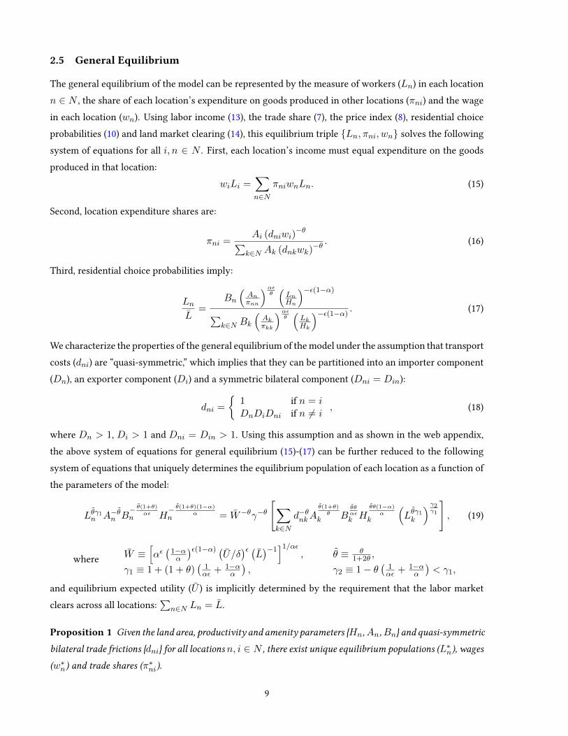
2.5 General Equilibrium

The general equilibrium of the model can be represented by the measure of workers (Ln) in each locationn ∈ N , the share of each location’s expenditure on goods produced in other locations (πni) and the wagein each location (wn). Using labor income (13), the trade share (7), the price index (8), residential choiceprobabilities (10) and land market clearing (14), this equilibrium triple Ln, πni, wn solves the followingsystem of equations for all i, n ∈ N . First, each location’s income must equal expenditure on the goodsproduced in that location:

wiLi =∑n∈N

πniwnLn. (15)

Second, location expenditure shares are:

πni =Ai (dniwi)

−θ∑k∈N Ak (dnkwk)

−θ . (16)

Third, residential choice probabilities imply:

LnL

=Bn

(Anπnn

)αεθ(LnHn

)−ε(1−α)∑

k∈N Bk

(Akπkk

)αεθ(LkHk

)−ε(1−α) . (17)

We characterize the properties of the general equilibrium of the model under the assumption that transportcosts (dni) are “quasi-symmetric,” which implies that they can be partitioned into an importer component(Dn), an exporter component (Di) and a symmetric bilateral component (Dni = Din):

dni =

1 if n = iDnDiDni if n 6= i

, (18)

where Dn > 1, Di > 1 and Dni = Din > 1. Using this assumption and as shown in the web appendix,the above system of equations for general equilibrium (15)-(17) can be further reduced to the followingsystem of equations that uniquely determines the equilibrium population of each location as a function ofthe parameters of the model:

Lθγ1n A−θn B− θ(1+θ)

αεn H

− θ(1+θ)(1−α)α

n = W−θγ−θ

[∑k∈N

d−θnkAθ(1+θ)θ

k Bθθαεk H

θθ(1−α)α

k

(Lθγ1k

) γ2γ1

], (19)

where W ≡[αε(1−αα

)ε(1−α) (U/δ

)ε (L)−1]1/αε

, θ ≡ θ1+2θ ,

γ1 ≡ 1 + (1 + θ)(

1αε + 1−α

α

), γ2 ≡ 1− θ

(1αε + 1−α

α

)< γ1,

and equilibrium expected utility (U ) is implicitly determined by the requirement that the labor marketclears across all locations:

∑n∈N Ln = L.

Proposition 1 Given the land area, productivity and amenity parameters Hn,An,Bn and quasi-symmetric

bilateral trade frictions dni for all locations n, i ∈ N , there exist unique equilibrium populations (L∗n), wages

(w∗n) and trade shares (π∗ni).

9

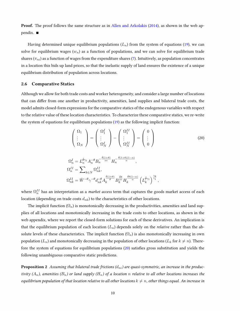
Proof. The proof follows the same structure as in Allen and Arkolakis (2014), as shown in the web ap-pendix.

Having determined unique equilibrium populations (Ln) from the system of equations (19), we cansolve for equilibrium wages (wn) as a function of populations, and we can solve for equilibrium tradeshares (πni) as a function of wages from the expenditure shares (7). Intuitively, as population concentratesin a location this bids up land prices, so that the inelastic supply of land ensures the existence of a uniqueequilibrium distribution of population across locations.

2.6 Comparative Statics

Although we allow for both trade costs and worker heterogeneity, and consider a large number of locationsthat can dier from one another in productivity, amenities, land supplies and bilateral trade costs, themodel admits closed-form expressions for the comparative statics of the endogenous variables with respectto the relative value of these location characteristics. To characterize these comparative statics, we re-writethe system of equations for equilibrium populations (19) as the following implicit function: Ω1

...ΩN

=

ΩI1

...ΩIN

− ΩII

1...ΩIIN

=

0...0

(20)

ΩIn = Lθγ1n A−θn B

− θ(1+θ)αε

n H− θ(1+θ)(1−α)

αn ,

ΩIIn =

∑k∈N

ΩIInk,

ΩIInk = W−θγ−θd−θnkA

θ(1+θ)θ

k Bθθαεk H

θθ(1−α)α

k

(Lθγ1k

) γ2γ1 ,

where ΩIIn has an interpretation as a market access term that captures the goods market access of each

location (depending on trade costs dnk) to the characteristics of other locations.The implicit function (Ωn) is monotonically decreasing in the productivities, amenities and land sup-

plies of all locations and monotonically increasing in the trade costs to other locations, as shown in theweb appendix, where we report the closed-form solutions for each of these derivatives. An implication isthat the equilibrium population of each location (Ln) depends solely on the relative rather than the ab-solute levels of these characteristics. The implicit function (Ωn) is also monotonically increasing in ownpopulation (Ln) and monotonically decreasing in the population of other locations (Lk for k 6= n). There-fore the system of equations for equilibrium populations (20) satises gross substitution and yields thefollowing unambiguous comparative static predictions.

Proposition 2 Assuming that bilateral trade frictions (dni) are quasi-symmetric, an increase in the produc-

tivity (An), amenities (Bn) or land supply (Hn) of a location n relative to all other locations increases the

equilibrium population of that location relative to all other locations k 6= n, other things equal. An increase in

10

location n’s trade costs to all other locations k 6= n (Dn) decreases the equilibrium population of that location

relative to all other locations k 6= n, other things equal.

Proof. See the web appendix.

Intuitively, locations with higher productivity, more attractive amenities, larger land supplies andlower trade costs attract larger populations, where the trade elasticity θ and the labor supply elasticityε inuence the sensitivity of equilibrium populations to variation in these characteristics.

2.7 Recovering Location Fundamentals

Given values for the model’s parameters α, θ, ε, a parameterization of bilateral trade costs dni and dataon populations, wages and land supplies Ln, wn, Hn, we now show that the solution to the generalequilibrium of the model can be used to recover the unobserved location characteristics of amenities (Bn)and productivities (An).

Proposition 3 Given the model parameters α, θ, ε, a parameterization of bilateral trade costs dni and

data on populations, wages and land supplies Ln, wn, Hn, there exist unique values of amenities (Bn) and

productivities (An) that are consistent with the data up to a normalization that corresponds to a choice of

units in which to measure amenities and productivities.

Proof. See the web appendix.

To solve for unobserved productivities and amenities, we use the recursive structure of the model. First,given data on population and wages Ln,wn, we can use the equality of income and expenditures (15) andtrade shares (16) to solve for the unobserved productivities An for which the endogenous variables arean equilibrium of the model. From these solutions for unobserved productivities An and population andwages Ln, wn, we immediately obtain trade shares πni. Second, given data on population and wagesLn, wn, we can use land market clearing (14) to solve for land rents rn. Third, given data on wages wnand the solutions for productivity and trade shares An, πni, we can use the relationship between priceindices and trade shares (8) to solve for price indices Pn. Finally, using data on population and wagesLn, wn and the solutions for land rents and price indices rn, Pn, we can use the residential choiceprobabilities (10) to solve for the unobserved amenities Bn for which the endogenous variables are anequilibrium of the model.

2.8 Counterfactuals

The system of equations for general equilibrium (15)-(17) provides an approach for undertaking model-based counterfactuals that uses only parameters and the values of endogenous variables in the initialequilibrium (as in Dekle, Eaton, and Kortum 2007). In contrast to standard trade models, these model-based counterfactuals yield predictions for the reallocation of labor across locations.

11

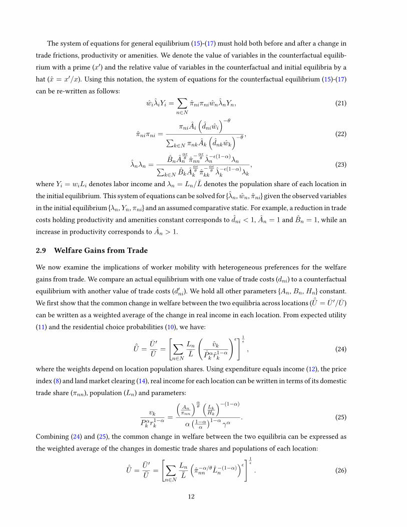
The system of equations for general equilibrium (15)-(17) must hold both before and after a change intrade frictions, productivity or amenities. We denote the value of variables in the counterfactual equilib-rium with a prime (x′) and the relative value of variables in the counterfactual and initial equilibria by ahat (x = x′/x). Using this notation, the system of equations for the counterfactual equilibrium (15)-(17)can be re-written as follows:

wiλiYi =∑n∈N

πniπniwnλnYn, (21)

πniπni =πniAi

(dniwi

)−θ∑

k∈N πnkAk

(dnkwk

)−θ , (22)

λnλn =BnA

αεθn π

−αεθ

nn λ−ε(1−α)n λn∑

k∈N BkAαεθk π

−αεθ

kk λ−ε(1−α)k λk

, (23)

where Yi = wiLi denotes labor income and λn = Ln/L denotes the population share of each location inthe initial equilibrium. This system of equations can be solved for λn, wn, πni given the observed variablesin the initial equilibrium λn, Yn, πni and an assumed comparative static. For example, a reduction in tradecosts holding productivity and amenities constant corresponds to dni < 1, An = 1 and Bn = 1, while anincrease in productivity corresponds to An > 1.

2.9 Welfare Gains from Trade

We now examine the implications of worker mobility with heterogeneous preferences for the welfaregains from trade. We compare an actual equilibrium with one value of trade costs (dni) to a counterfactualequilibrium with another value of trade costs (d′ni). We hold all other parameters An, Bn, Hn constant.We rst show that the common change in welfare between the two equilibria across locations ( ˆU = U ′/U )can be written as a weighted average of the change in real income in each location. From expected utility(11) and the residential choice probabilities (10), we have:

ˆU =U ′

U=

[∑n∈N

LnL

(vk

Pαk r1−αk

)ε] 1ε

, (24)

where the weights depend on location population shares. Using expenditure equals income (12), the priceindex (8) and land market clearing (14), real income for each location can be written in terms of its domestictrade share (πnn), population (Ln) and parameters:

vk

Pαk r1−αk

=

(Anπnn

)αθ(LkHk

)−(1−α)α(1−αα

)1−αγα

. (25)

Combining (24) and (25), the common change in welfare between the two equilibria can be expressed asthe weighted average of the changes in domestic trade shares and populations of each location:

ˆU =U ′

U=

[∑n∈N

LnL

(π−α/θnn L−(1−α)n

)ε] 1ε

. (26)

12

While this expression features the changes in the domestic trade shares and populations of all locations, wenow show that welfare also can be expressed in terms of the characteristics of any one individual location.From expected utility (11), the residential choice probabilities (10) and real income (25), the common levelof utility across locations can be expressed as:

Un = U =δB

1εn

(Anπnn

)αθH1−αn L

−( 1ε+(1−α))

n

α(1−αα

)1−αγα(L)− 1

ε

, ∀ n. (27)

Population mobility implies that this relationship must hold for each location. Locations with higherproductivity (An), better amenities (Bn), better goods market access to other locations (lower πnn) andhigher supplies of land (Hn) have higher populations, which bids up the price of land until expected utilityconditional on living in each location is the same for all locations.

An implication of this result is that the domestic trade share in the open economy equilibrium (πTnn),populations in the closed and open economies (LAn and LTn ), the trade elasticity (θ), the elasticity of popu-lation supply with respect to real income (ε) and the consumption goods share (α) are sucient statisticsfor the welfare gains from trade:

UTnUAn

=UT

UA=

(1

πTnn

)αθ(LAnLTn

) 1ε+(1−α)

, ∀ n, (28)

where we use the superscript T to denote the trade equilibrium and the superscriptA to denote the autarkyequilibrium; we have used πAnn = 1; and in general LAn 6= LTn .

Intuitively, if some locations have better market access than others in the open economy (as reectedin a lower open economy domestic trade share πTnn), the opening of goods trade will lead to a largerreduction in the consumption price index in these locations. This larger reduction in the consumptionprice index in turn creates an incentive for migration from locations with worse market access to thosewith better market access. This labor mobility provides the mechanism that restores equilibrium, as theprice of land is bid up in locations with better market access and bid down in those with worse marketaccess, until expected utility is equalized across all locations. Therefore, computing the common valuefor the welfare gains from trade across all locations involves taking into account not only domestic tradeshares (which aect consumption price indices) but also population redistributions (which aect the priceof the immobile factor land).

One special case of the model is perfect labor mobility and no preference heterogeneity (ε → ∞), inwhich case there is a perfectly elastic supply of labor to each location at the common real wage. As shownin the web appendix, in this case the common welfare gains from trade across all locations again dependon the domestic trade share in the open economy equilibrium (πTnn) and populations in the closed andopen economies (LAn and LTn ):

UTnUAn

=UT

UA=

(1

πTnn

)αθ(LAnLTn

)1−α

, ∀ n, (29)

13

which corresponds to a special case of (28) as ε→∞.A second special case of the model is perfect labor immobility, in which case expected utility in gen-

eral diers across locations, because population reallocations no longer provide a mechanism for utilityequalization through changes in the price of land. As shown in the web appendix, in this case the welfaregains from trade in general dier across locations and depend solely on the domestic trade share in theopen economy equilibrium (πTnn) for each location:

UTnUAn

=

(1

πTnn

)αθ

6=UTkUAk

, n 6= k, (30)

which corresponds to a special case of (28) in which LAn = LTn because of labor immobility.

3 Agglomeration Forces

In this section, we examine the implications of introducing agglomeration forces in our setting with bothtrade costs and labor mobility with heterogeneous worker preferences. These agglomeration forces takethe form of pecuniary externalities as a result of transport costs, increasing returns to scale and love ofvariety, as in the new economic geography literature following Krugman (1991a,b), Krugman and Ven-ables (1995) and Helpman (1998), and synthesized in Fujita, Krugman, and Venables (1999). This literaturetypically restricts attention to stylized settings with a small number of symmetric locations and assumeseither a perfectly inelastic supply of labor to each location, a perfectly elastic supply of labor to each lo-cation, or a mechanical relationship between migration ows and relative wages. In contrast, we considera rich geography with a large number of asymmetric locations, and allow for a positive nite elasticity oflabor supply to each location.

3.1 Consumer Preferences

Preferences are again dened over goods consumption (Cn) and residential land use (HUn) and take thesame form as in (1). The goods consumption index (Cn), however, is now dened over the endogenousmeasures of horizontally dierentiated varieties supplied by each location (Mi):

Cn =

[∑i∈N

∫ Mi

0cni (j)ρ dj

] 1ρ

, (31)

where trade between locations i and n is again subject to iceberg variable trade costs of dni ≥ 1.

3.2 Production

Varieties are produced under conditions of monopolistic competition and increasing returns to scale. Toproduce a variety, a rm must incur a xed cost of F units of labor and a constant variable cost in termsof labor that depends on a location’s productivity Ai. Therefore the total amount of labor (li(j)) required

14

to produce xi(j) units of a variety j in location i is:

li(j) = F +xi(j)

Ai. (32)

Prot maximization and zero prots imply that equilibrium prices are a constant mark-up over marginalcost:

pni(j) =

(σ

σ − 1

)dniwiAi

, (33)

and equilibrium employment for each variety is equal to a constant:

li(j) = l = σF. (34)

Given this constant equilibrium employment for each variety, labor market clearing implies that the to-tal measure of varieties supplied by each location is proportional to the endogenous supply of workerschoosing to locate there:

Mi =LiσF

. (35)

3.3 Expenditure Shares and Price Indices

Using the CES expenditure function, equilibrium prices (33) and labor market clearing (35), the share oflocation n’s expenditure on goods produced in location i is:

πni =Li

(dniwiAi

)1−σ∑

k∈N Lk

(dnkwkAk

)1−σ , (36)

where the elasticity of trade with respect to trade costs is now determined by the elasticity of substitution(σ − 1). Furthermore, trade shares now depend directly on population (Li) because this determines theendogenous measure of varieties produced by a location through the labor market clearing condition (35).

Using equilibrium prices (33), labor market clearing (35), the trade share (36) and dnn = 1, the con-sumption goods price index can be written as:

P 1−σn =

LnσFπnn

(σ

σ − 1

wnAn

)1−σ, (37)

which again depends directly on population (Ln) through the endogenous measure of varieties.

3.4 Residential Choices and Income

Residential choices take a similar form as in section 2. Using the Fréchet distribution of idiosyncraticshocks to amenities, the probability that a worker chooses to live in location n ∈ N is:

LnL

=Bn(vn/P

αn r

1−αn

)ε∑k∈N Bk

(vk/P

αk r

1−αk

)ε , (38)

15

where the elasticity of population with respect to real income is again determined by the Fréchet shapeparameter for consumer tastes ε. Expected worker utility is:

U = δ

[∑k∈N

Bk(vk/P

αk r

1−αk

)ε] 1ε

, (39)

where δ = Γ ((ε− 1)/ε); Γ (·) is the Gamma function; and ε > 1. The Fréchet distribution of utility againimplies that expected utility conditional on residing in location n is the same across all locations n andequal to expected utility for the economy as a whole.

Expenditure on land in each location is redistributed lump sum to the workers residing in that location,which implies that total income (vn) equals labor income plus expenditure on residential land (as in (12)).Land market clearing implies that the equilibrium land rent again can be determined from the equality ofland income and expenditure (as in (14)).

3.5 General Equilibrium

The general equilibrium of the model can be represented by the measure of workers (Ln) in each locationn ∈ N , the share of each location’s expenditure on goods produced by other locations (πni) and the wagein each location (wn). We again characterize the properties of the general equilibrium of the model underthe assumption that transport costs (dni) are “quasi-symmetric”:

dni =

1 if n = iDnDiDni if n 6= i

, (40)

whereDn > 1,Di > 1 andDni = Din > 1. Under this assumption and as shown in the web appendix, thesystem of equations for general equilibrium can be further reduced to the following system of equationsthat uniquely determines the equilibrium population of each location as a function of parameters:

Lσγ1n A−σ(σ−1)n B− σσ

αεn H

− σσ(1−α)α

n = W 1−σ

[∑k∈N

1

σF

(σdnkσ − 1

)1−σ

Aσσk Bσ(σ−1)

αε

k Hσ(σ−1)(1−α)

α

k

(Lσγ1k

) γ2γ1

], (41)

where W ≡

[αε(

1− αα

)ε(1−α) (U/δ

)ε (L)−1]1/αε

, σ ≡ σ − 1

2σ − 1,

1− αα≡(

1

αε+

1− αα

),

α ≡ α

1 + 1ε

, γ1 ≡ σ(

1− αα

), γ2 ≡ 1 +

σ

σ − 1− (σ − 1)

(1− αα

),

and equilibrium expected utility (U ) is implicitly determined by the requirement that the labor marketclears across all locations:

∑n∈N Ln = L. The condition for there to exist a unique stable equilibrium is:

σ (1− α) > 1, ⇔ γ2γ1

< 1. (42)

In the special case of the model in which there is no dispersion in idiosyncratic shocks to amenities (ε→∞), this condition for a unique equilibrium reduces to the condition in the new economic geography modelof Helpman (1998) for the case of two regions and no worker heterogeneity of σ (1− α) > 1.

16

Proposition 4 Assume σ (1− α) > 1. Given the land area, productivity and amenity parameters Hn,

An, Bn and quasi-symmetric bilateral trade frictions dni for all locations n, i ∈ N , there exist unique

equilibrium populations (L∗n), trade shares (π∗ni) and wages (w

∗n).

Proof. The proof follows the same structure as in Allen and Arkolakis (2014), as shown in the web ap-pendix.

Intuitively, as population concentrates in a location, this expands the measure of varieties producedthere, which in the presence of trade costs makes that location a more attractive residence (an agglomer-ation force). However, as population concentrates in a location, this also bids up land prices (a dispersionforce). As long as the parameter inequality (42) is satised, the dispersion force dominates the agglomer-ation force, which ensures the existence of a unique equilibrium distribution of economic activity.

3.6 Comparative Statics

Despite the introduction of agglomeration forces in a setting with a large number of asymmetric loca-tions, the model continues to admit closed-form expressions for the comparative statics of the endogenousvariables with respect to the relative value of location characteristics. To characterize these comparativestatics, we re-write the system of equations for equilibrium populations (41) as the implicit function: Ω1

...ΩN

=

ΩI1

...ΩIN

− ΩII

1...ΩIIN

=

0...0

(43)

ΩIn = Lσγ1n A−σ(σ−1)n B

− σσαε

n H− σσ(1−α)

αn ,

ΩIIn =

∑k∈N

ΩIInk,

ΩIInk = W 1−σ 1

σF

(σdnkσ − 1

)1−σAσσk B

σ(σ−1)αε

k Hσ(σ−1)(1−α)

αk

(Lσγ1k

) γ2γ1 ,

where ΩIIn has an interpretation as a market access term that captures the goods market access of each

location (depending on trade costs dnk) to the characteristics of other locations.The system of equations for equilibrium populations (43) exhibits similar properties as in Section 2.6

and satises gross substitution, which yields the following unambiguous comparative static predictions.

Proposition 5 Assuming σ (1− α) > 1 and quasi-symmetric bilateral trade frictions (dni), an increase

in the productivity (An), amenities (Bn) or land supply (Hn) of a location n relative to all other locations

increases the equilibrium population of that location relative to all other locations k 6= n, other things equal.

An increase in location n’s trade costs to all other locations k 6= n (Dn) decreases the equilibrium population

of that location relative to all other locations k 6= n, other things equal.

17

Proof. See the web appendix.

Intuitively, locations with higher productivity, more attractive amenities, larger land supplies andlower trade costs attract larger populations, where the trade elasticity (σ − 1) and the labor supply elas-ticity ε inuence the sensitivity of equilibrium populations to variation in these characteristics.

3.7 Recovering Location Fundamentals

Given values for the model’s parameters α, θ, ε, a parameterization of bilateral trade costs dni anddata on populations, wages and land supplies Ln, wn, Hn, we now show that the solution to the generalequilibrium of the model again can be used to recover the unobserved location characteristics of amenities(Bn) and productivities (An).

Proposition 6 Given the model parameters α, σ, ε, a parameterization of bilateral trade costs dni and

data on populations, wages and land supplies Ln, wn, Hn, there exist unique values of amenities (Bn) and

productivities (An) that are consistent with the data up to a normalization that corresponds to a choice of

units in which to measure amenities and productivities.

Proof. See the web appendix.

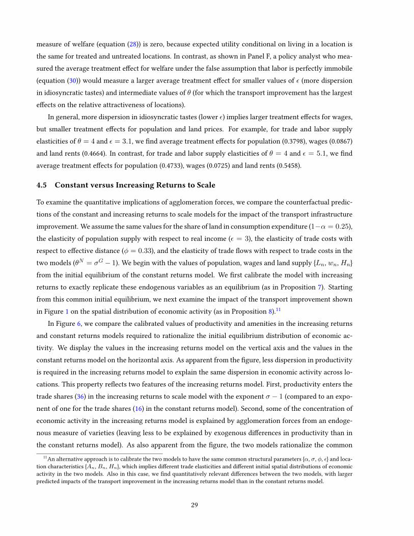
From Propositions 3 and 6, the constant and increasing returns models can be both calibrated to repli-cate the same data on populations, wages and land supplies Ln, wn, Hn. In the constant returns model,the elasticity of trade with respect to variable trade costs is determined by the shape parameter of theproductivity distribution (θN > σN − 1), where the subscript N (neoclassical) indicates the constantreturns model. In contrast, in the increasing returns model, the trade elasticity is dictated by the elas-ticity of substitution between varieties (σG − 1), where the superscript G indicates the increasing re-turns to scale (new economic geography) model. Therefore calibrating both models to the same initialequilibrium and trade elasticities requires dierent structural parameters for the elasticity of substitution(σG − 1 = θN > σN − 1). Furthermore, population directly aects the trade shares in the increasingreturns model (36), but does not directly aect the trade shares in the constant returns model (16). There-fore calibrating both models to the same initial equilibrium also requires assuming dierent unobservedproductivities in the two models, as summarized in the following proposition.

Proposition 7 Given the parameters α, ε and θN = σG−1, and given a parameterization of bilateral trade

costs dni, the constant returns model (superscript N ) and increasing returns model (superscript G) both can

be calibrated to the same data on populations, wages and land supplies Ln, wn,Hn in an initial equilibrium.

This calibration involves dierent structural parameters (σN 6= σG) and productivities (ANn 6= AGn ) but the

same amenities (BNn = BG

n ) in the two models.

Proof. See the web appendix.

18

Given the dierent structural parameters and productivities, the constant and increasing returns mod-els both rationalize the same data on the endogenous variables of the model as an equilibrium.

3.8 Counterfactuals

The system of equations for general equilibrium again provides an approach for undertaking model-basedcounterfactuals that uses only parameters and the values of endogenous variables in an initial equilibrium.Denoting the relative value of variables in the counterfactual and initial equilibria by a hat (x = x′/x), wecan solve for the counterfactual eects of a change in trade costs, productivity or amenities using:

wiλiYi =∑n∈N

πniπniwnλnYn, (44)

πniπni =πni

(dniwi/Ai

)1−σλi∑

k∈N πnk

(dnkwk/Ak

)1−σλk

, (45)

λnλn =BnA

αεn π− αεσ−1

nn λ−(ε(1−α)− αε

σ−1)n λn∑

k∈N BkAαεk π− αεσ−1

kk λ−(ε(1−α)− αε

σ−1)k λk

. (46)

where Yi = wiLi again denotes labor income and λn = Ln/L denotes the population share of eachlocation in the initial equilibrium. This system of equations can be solved for λn, wn, πni given theobserved variables in the initial equilibrium λn, Yn, πni and an assumed comparative static.

Comparing the counterfactual systems in the constant returns model ((21)-(23)) and the increasingreturns model ((44)-(46)), the dependence of the measures of varieties on populations in the increasingreturns model is reected in both the trade shares (in the terms in Li in (45)) and the residential choiceprobabilities (in the dierent exponents on Li in (46) compared to (23)). This dependence of the measureof varieties on the endogenous populations of locations in the increasing returns model implies dierentcounterfactual predictions for the impact of changes in trade costs from the constant returns model. Thesedierences exist even if the two models are calibrated to the same initial equilibrium wn, Ln, πni, thesame trade elasticity (θN = σG − 1), and the same values of the other model parameters.

Proposition 8 Suppose that the constant and increasing returns to scale models are calibrated to the same

data on populations, wages and land supplies Ln, wn, Hn in an initial equilibrium with the same trade

elasticity θN = σG − 1 and the same values of the other model parameters. Even when calibrated in this

way, the two models imply dierent counterfactual predictions for the eects of a reduction in trade costs on

population, wages, trade shares and welfare Ln, wn, πni, U .

Proof. See the web appendix.

In an international trade context, in which population is immobile between locations, these two modelsimply the same counterfactual predictions for the eects of a reduction in trade costs on wages, trade

19

shares and welfare (see Arkolakis, Costinot, and Rodriguez-Clare 2012). In contrast, in a setting in whichlabor is mobile across locations, the reallocation of population across locations in response to the reductionin trade costs leads to dierent counterfactual predictions in the two models.

3.9 Welfare Gains from Trade

We now examine the implications of the introduction of agglomeration forces for the welfare gains fromtrade. Using the residential choice probabilities (38), expected utility (39), income equals expenditure (12),land market clearing (14) and the goods price index (37), the common level of utility across all locationscan be expressed in terms of the characteristics of any one individual location:

U =δB

1εnAαn

(1πnn

) ασ−1

H1−αn L

−( 1ε+(1−α)− α

σ−1)n

α(1−αα

)1−α ( σσ−1

)α(σF )

ασ−1

(L)− 1

ε

, (47)

where the condition for the existence of a unique equilibrium σ (1− α) > 1 implies that the expectedutility for each location is decreasing in its population (1ε + (1 − α) > α

σ−1 ). The domestic trade share(πnn), population (Ln), the trade elasticity (σ − 1), the population supply elasticity (ε) and the share oftradables in expenditure (α) are again sucient statistics for the welfare gains from trade:

UT

UA=

(1

πTnn

) ασ−1

(LAnLTn

) 1ε+(1−α)− α

σ−1

. (48)

In this expression for the welfare gains from trade in the increasing returns model (48), the exponenton relative populations now has an additional term (−α/(σ − 1)) that captures the impact of populationon the endogenous measure of varieties (absent in the constant returns model in the previous section).Furthermore, from Proposition 8, the two models have dierent counterfactual predictions for the eects ofreductions in trade costs on domestic trade shares and populations, even when calibrated to the same initialequilibrium. Therefore the two models have dierent implications for the welfare gains from reductionsin trade costs, as explored further below. As in the case of the neoclassical model considered in Section2.9, the cases of a perfectly elastic and perfectly inelastic supplies of labor to each location are both specialcases of this framework, as shown in the web appendix.

4 Quantitative Analysis

To examine the quantitative properties of this class of spatial equilibrium models, we rst assume param-eter values and generate data for a hypothetical economy for the constant returns model from Section 2.Second, we examine the implications of a reduction in trade costs on the spatial organization of economicactivity within the constant returns model. Third, we compare this impact of the reduction in trade costsin the constant returns model to that in the increasing returns model from Section 3.

20

4.1 Model Economy

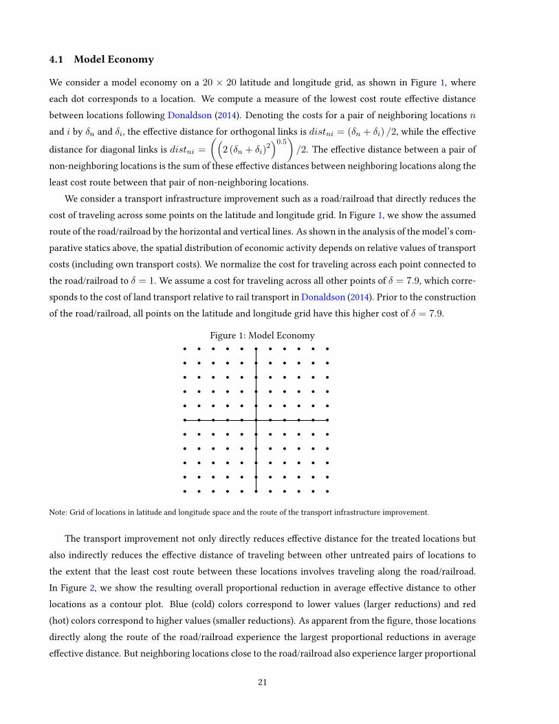
We consider a model economy on a 20 × 20 latitude and longitude grid, as shown in Figure 1, whereeach dot corresponds to a location. We compute a measure of the lowest cost route eective distancebetween locations following Donaldson (2014). Denoting the costs for a pair of neighboring locations nand i by δn and δi, the eective distance for orthogonal links is distni = (δn + δi) /2, while the eective

distance for diagonal links is distni =

((2 (δn + δi)

2)0.5)

/2. The eective distance between a pair ofnon-neighboring locations is the sum of these eective distances between neighboring locations along theleast cost route between that pair of non-neighboring locations.

We consider a transport infrastructure improvement such as a road/railroad that directly reduces thecost of traveling across some points on the latitude and longitude grid. In Figure 1, we show the assumedroute of the road/railroad by the horizontal and vertical lines. As shown in the analysis of the model’s com-parative statics above, the spatial distribution of economic activity depends on relative values of transportcosts (including own transport costs). We normalize the cost for traveling across each point connected tothe road/railroad to δ = 1. We assume a cost for traveling across all other points of δ = 7.9, which corre-sponds to the cost of land transport relative to rail transport in Donaldson (2014). Prior to the constructionof the road/railroad, all points on the latitude and longitude grid have this higher cost of δ = 7.9.

Figure 1: Model Economy

rrrrrrrrrrr

rrrrrrrrrrr

rrrrrrrrrrr

rrrrrrrrrrr

rrrrrrrrrrr

rrrrrrrrrrr

rrrrrrrrrrr

rrrrrrrrrrr

rrrrrrrrrrr

rrrrrrrrrrr

rrrrrrrrrrr

Note: Grid of locations in latitude and longitude space and the route of the transport infrastructure improvement.

The transport improvement not only directly reduces eective distance for the treated locations butalso indirectly reduces the eective distance of traveling between other untreated pairs of locations tothe extent that the least cost route between these locations involves traveling along the road/railroad.In Figure 2, we show the resulting overall proportional reduction in average eective distance to otherlocations as a contour plot. Blue (cold) colors correspond to lower values (larger reductions) and red(hot) colors correspond to higher values (smaller reductions). As apparent from the gure, those locationsdirectly along the route of the road/railroad experience the largest proportional reductions in averageeective distance. But neighboring locations close to the road/railroad also experience larger proportional

21

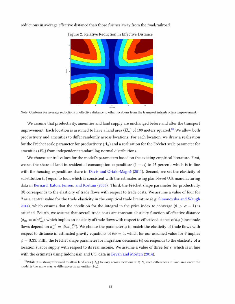
reductions in average eective distance than those further away from the road/railroad.

Figure 2: Relative Reduction in Eective Distance

Longitude

Latit

ude

2 4 6 8 10

2

4

6

8

10

Note: Contours for average reductions in eective distance to other locations from the transport infrastructure improvement.

We assume that productivity, amenities and land supply are unchanged before and after the transportimprovement. Each location is assumed to have a land area (Hn) of 100 meters squared.10 We allow bothproductivity and amenities to dier randomly across locations. For each location, we draw a realizationfor the Fréchet scale parameter for productivity (An) and a realization for the Fréchet scale parameter foramenities (Bn) from independent standard log normal distributions.

We choose central values for the model’s parameters based on the existing empirical literature. First,we set the share of land in residential consumption expenditure (1 − α) to 25 percent, which is in linewith the housing expenditure share in Davis and Ortalo-Magné (2011). Second, we set the elasticity ofsubstitution (σ) equal to four, which is consistent with the estimates using plant-level U.S. manufacturingdata in Bernard, Eaton, Jensen, and Kortum (2003). Third, the Fréchet shape parameter for productivity(θ) corresponds to the elasticity of trade ows with respect to trade costs. We assume a value of four forθ as a central value for the trade elasticity in the empirical trade literature (e.g. Simonovska and Waugh2014), which ensures that the condition for the integral in the price index to converge (θ > σ − 1) issatised. Fourth, we assume that overall trade costs are constant elasticity function of eective distance(dni = distφni), which implies an elasticity of trade ows with respect to eective distance of θφ (since tradeows depend on d−θni = dist−θφni ). We choose the parameter φ to match the elasticity of trade ows withrespect to distance in estimated gravity equations of θφ = 1, which for our assumed value for θ impliesφ = 0.33. Fifth, the Fréchet shape parameter for migration decisions (ε) corresponds to the elasticity of alocation’s labor supply with respect to its real income. We assume a value of three for ε, which is in linewith the estimates using Indonesian and U.S. data in Bryan and Morten (2014).

10While it is straightforward to allow land area (Hn) to vary across locations n ∈ N , such dierences in land area enter themodel is the same way as dierences in amenities (Bn).

22

4.2 Reduction in Transport Costs

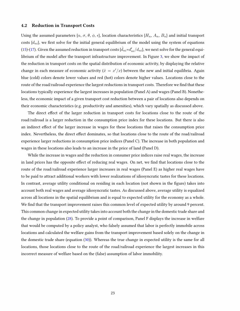
Using the assumed parameters α, σ, θ, φ, ε, location characteristics Hn, An, Bn and initial transportcosts dni, we rst solve for the initial general equilibrium of the model using the system of equations(15)-(17). Given the assumed reduction in transport costs dni=d′ni/dni, we next solve for the general equi-librium of the model after the transport infrastructure improvement. In Figure 3, we show the impact ofthe reduction in transport costs on the spatial distribution of economic activity, by displaying the relativechange in each measure of economic activity (x = x′/x) between the new and initial equilibria. Againblue (cold) colors denote lower values and red (hot) colors denote higher values. Locations close to theroute of the road/railroad experience the largest reductions in transport costs. Therefore we nd that theselocations typically experience the largest increases in population (Panel A) and wages (Panel B). Nonethe-less, the economic impact of a given transport cost reduction between a pair of locations also depends ontheir economic characteristics (e.g. productivity and amenities), which vary spatially as discussed above.

The direct eect of the larger reduction in transport costs for locations close to the route of theroad/railroad is a larger reduction in the consumption price index for these locations. But there is alsoan indirect eect of the larger increase in wages for these locations that raises the consumption priceindex. Nevertheless, the direct eect dominates, so that locations close to the route of the road/railroadexperience larger reductions in consumption price indices (Panel C). The increase in both population andwages in these locations also leads to an increase in the price of land (Panel D).

While the increase in wages and the reduction in consumer price indices raise real wages, the increasein land prices has the opposite eect of reducing real wages. On net, we nd that locations close to theroute of the road/railroad experience larger increases in real wages (Panel E) as higher real wages haveto be paid to attract additional workers with lower realizations of idiosyncratic tastes for these locations.In contrast, average utility conditional on residing in each location (not shown in the gure) takes intoaccount both real wages and average idiosyncratic tastes. As discussed above, average utility is equalizedacross all locations in the spatial equilibrium and is equal to expected utility for the economy as a whole.We nd that the transport improvement raises this common level of expected utility by around 9 percent.This common change in expected utility takes into account both the change in the domestic trade share andthe change in population (28). To provide a point of comparison, Panel F displays the increase in welfarethat would be computed by a policy analyst, who falsely assumed that labor is perfectly immobile acrosslocations and calculated the welfare gains from the transport improvement based solely on the change inthe domestic trade share (equation (30)). Whereas the true change in expected utility is the same for alllocations, those locations close to the route of the road/railroad experience the largest increases in thisincorrect measure of welfare based on the (false) assumption of labor immobility.

23

Figure 3: Relative Changes (x = x′/x) Following the Transport Improvement

Longitude

Latit

ude

Panel A : Population

2 4 6 8 10

2

4

6

8

10

Longitude

Latit

ude

Panel B : Wages

2 4 6 8 10

2

4

6

8

10

Longitude

Latit

ude

Panel C : Price Index

2 4 6 8 10

2

4

6

8

10

Longitude

Latit

ude

Panel D : Land Rents

2 4 6 8 10

2

4

6

8

10

Longitude

Latit

ude

Panel E : Real Wage

2 4 6 8 10

2

4

6

8

10

Longitude

Latit

ude

Panel F : Incorrect Immobile Welfare

2 4 6 8 10

2

4

6

8

10

Note: Contours for relative changes in economic activity in the constant returns model following the transport improvement.

4.3 Treatment Eects of the Transport Improvement

A growing empirical literature uses quasi-experimental variation in transport infrastructure investmentsto estimate the reduced-form impact of these investments on the spatial distribution of economic activity(see for example Michaels 2008, Duranton and Turner 2012 and the review in Redding and Turner 2015).Although most of this literature focuses on estimating average treatment eects, Donaldson and Hornbeck(2016) examines the eects of the U.S. railroad network on county land values through changes in marketaccess. A key implication of our model is that the transport infrastructure improvement has heterogeneoustreatment eects across locations. Among the treated locations, those closest to the intersection of thehorizontal and vertical lines in Figure 1, experience the largest reductions in transport costs. Amongthe untreated locations that are not directly aected by the transport infrastructure, many are indirectlyaected by it because it reduces transport costs along the least cost route to other locations (Figure 2). Wenow examine the quantitative relevance of these heterogeneous treatment eects in the model.

In our model economy in Figure 1, the route for the transport infrastructure improvement was ex-ogenously assigned. Therefore we use this quasi-experimental variation to estimate the impact of thistransport infrastructure improvement on the spatial distribution of economy activity within the model.Under exogenous assignment, the causal impact of the transport infrastructure improvement can be esti-

24

mated using the following “dierences-in-dierences” specication:

lnYnt = ϑn + βInt + dt + unt, (49)

where n indexes locations and t indexes periods (before and after the transport improvement); Ynt is aneconomic outcome of interest (e.g. population); Int is an indicator variable that is one if a location istreated with transport infrastructure and zero otherwise; treatment is dened in terms of a location beingdirectly aected by the transport infrastructure improvement; ϑn are location xed eects; dt are periodxed eects; and unt is a stochastic error. The inclusion of both sets of xed eects ensures a “dierences-in-dierences” interpretation, where the rst dierence is between treated and untreated locations andthe second dierence is before and after the transport improvement.

Taking dierences in (49) before and after the transport infrastructure improvement, we obtain thefollowing “long dierences” specication:

4 lnYnt = ν + βInt + ent, (50)

where the location xed eects have now dierenced out and with only two periods the change in theperiod xed eects is captured in the regression constant ν.

In Column (1) of Table 1, we report the results of estimating the long dierences specication (50)for the transport infrastructure improvement shown in Figure 1. Consistent with the reorientation of thespatial distribution of economic activity shown in Figure 3, we nd positive average treatment eectsfor population and wages, a negative average treatment eect for the price index, and positive averagetreatment eects for land rents, real wages and the incorrect measure of welfare based on the (false)assumption of labor immobility. However, as apparent from Figure 3, these estimated average treatmenteects mask considerable heterogeneity in the impact of the transport improvement.

In Figure 4, we provide further evidence on these heterogeneous treatment eects by displaying thedistributions of the relative changes (x = x′/x) in the economic outcomes shown in Figure 3 as his-tograms across twenty equally-spaced bins. We show the distributions for treated locations (in black) anduntreated locations (in light blue) separately. As apparent from the gure, we nd considerable hetero-geneity among both groups of locations. Heterogeneity in access to transport infrastructure among thetreated locations and in the indirect eects of the transport infrastructure among the untreated locationsimply that the smallest positive changes for the treated locations are close to the largest positive changesfor the untreated locations. For example, for population, the relative change among treated locationsvaries from 1.6 to less than 1.2, while the relative change among untreated locations varies from 0.9 tomore than 1.1. Therefore, for central parameter values from the existing empirical literature, the modelimplies quantitatively relevant heterogeneous treatment eects.

As discussed above, the true relative change in welfare as a result of the transport improvement (equa-tion (28)) is the same across all locations. Therefore, the treatment eect for true welfare (not reported inTable 1) is zero, because there is no dierential change between treated and untreated locations. In con-trast, a policy analyst who measured the relative change in welfare under the false assumption of perfect

25

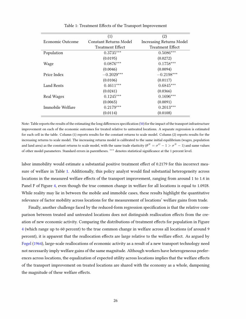
Table 1: Treatment Eects of the Transport Improvement

(1) (2)Economic Outcome Constant Returns Model Increasing Returns Model

Treatment Eect Treatment EectPopulation 0.3735∗∗∗ 0.5086∗∗∗

(0.0195) (0.0272)Wage 0.0876∗∗∗ 0.1758∗∗∗

(0.0046) (0.0094)Price Index −0.2029∗∗∗ −0.2198∗∗∗

(0.0106) (0.0117)Land Rents 0.4611∗∗∗ 0.6845∗∗∗

(0.0241) (0.0366)Real Wages 0.1245∗∗∗ 0.1696∗∗∗

(0.0065) (0.0091)Immobile Welfare 0.2179∗∗∗ 0.2013∗∗∗

(0.0114) (0.0108)

Note: Table reports the results of the estimating the long dierences specication (50) for the impact of the transport infrastructureimprovement on each of the economic outcomes for treated relative to untreated locations. A separate regression is estimatedfor each cell in the table. Column (1) reports results for the constant returns to scale model. Column (2) reports results for theincreasing returns to scale model. The increasing returns model is calibrated to the same initial equilibrium (wages, populationand land area) as the constant returns to scale model, with the same trade elasticity (θN = σG − 1 > σN − 1) and same valuesof other model parameters. Standard errors in parentheses. ∗∗∗ denotes statistical signicance at the 1 percent level.

labor immobility would estimate a substantial positive treatment eect of 0.2179 for this incorrect mea-sure of welfare in Table 1. Additionally, this policy analyst would nd substantial heterogeneity acrosslocations in the measured welfare eects of the transport improvement, ranging from around 1 to 1.4 inPanel F of Figure 4, even though the true common change in welfare for all locations is equal to 1.0928.While reality may lie in between the mobile and immobile cases, these results highlight the quantitativerelevance of factor mobility across locations for the measurement of locations’ welfare gains from trade.

Finally, another challenge faced by the reduced-form regression specication is that the relative com-parison between treated and untreated locations does not distinguish reallocation eects from the cre-ation of new economic activity. Comparing the distributions of treatment eects for population in Figure4 (which range up to 60 percent) to the true common change in welfare across all locations (of around 9percent), it is apparent that the reallocation eects are large relative to the welfare eect. As argued byFogel (1964), large-scale reallocations of economic activity as a result of a new transport technology neednot necessarily imply welfare gains of the same magnitude. Although workers have heterogeneous prefer-ences across locations, the equalization of expected utility across locations implies that the welfare eectsof the transport improvement on treated locations are shared with the economy as a whole, dampeningthe magnitude of these welfare eects.

26

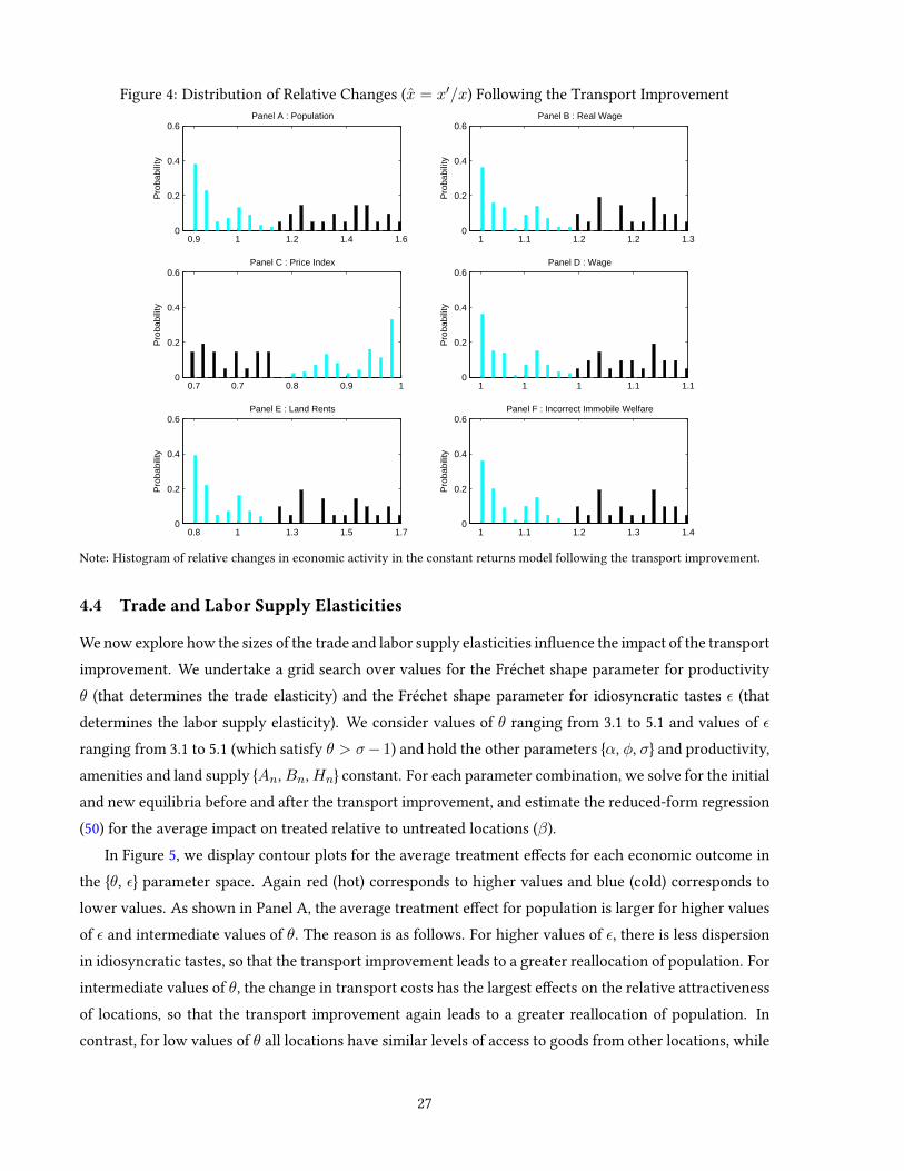
Figure 4: Distribution of Relative Changes (x = x′/x) Following the Transport Improvement

0.9 1 1.2 1.4 1.60

0.2

0.4

0.6

Pro

babi

lity

Panel A : Population

1 1.1 1.2 1.2 1.30

0.2

0.4

0.6

Pro

babi

lity

Panel B : Real Wage

0.7 0.7 0.8 0.9 10

0.2

0.4

0.6

Pro

babi

lity

Panel C : Price Index

1 1 1 1.1 1.10

0.2

0.4

0.6

Pro

babi

lity

Panel D : Wage

0.8 1 1.3 1.5 1.70

0.2

0.4

0.6

Pro

babi

lity

Panel E : Land Rents

1 1.1 1.2 1.3 1.40

0.2

0.4

0.6

Pro

babi

lity

Panel F : Incorrect Immobile Welfare

Note: Histogram of relative changes in economic activity in the constant returns model following the transport improvement.

4.4 Trade and Labor Supply Elasticities

We now explore how the sizes of the trade and labor supply elasticities inuence the impact of the transportimprovement. We undertake a grid search over values for the Fréchet shape parameter for productivityθ (that determines the trade elasticity) and the Fréchet shape parameter for idiosyncratic tastes ε (thatdetermines the labor supply elasticity). We consider values of θ ranging from 3.1 to 5.1 and values of εranging from 3.1 to 5.1 (which satisfy θ > σ− 1) and hold the other parameters α, φ, σ and productivity,amenities and land supply An,Bn,Hn constant. For each parameter combination, we solve for the initialand new equilibria before and after the transport improvement, and estimate the reduced-form regression(50) for the average impact on treated relative to untreated locations (β).

In Figure 5, we display contour plots for the average treatment eects for each economic outcome inthe θ, ε parameter space. Again red (hot) corresponds to higher values and blue (cold) corresponds tolower values. As shown in Panel A, the average treatment eect for population is larger for higher valuesof ε and intermediate values of θ. The reason is as follows. For higher values of ε, there is less dispersionin idiosyncratic tastes, so that the transport improvement leads to a greater reallocation of population. Forintermediate values of θ, the change in transport costs has the largest eects on the relative attractivenessof locations, so that the transport improvement again leads to a greater reallocation of population. Incontrast, for low values of θ all locations have similar levels of access to goods from other locations, while

27

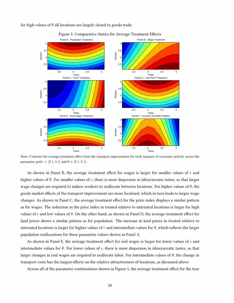
for high values of θ all locations are largely closed to goods trade.

Figure 5: Comparative Statics for Average Treatment Eects

Theta

Eps

ilon

Panel A : Population Treatment

3.5 4 4.5 5

3.5

4

4.5

5

Theta

Eps

ilon

Panel B : Wage Treatment

3.5 4 4.5 5

3.5

4

4.5

5

Theta

Eps

ilon

Panel C : Price Treatment

3.5 4 4.5 5

3.5

4

4.5

5

ThetaE

psilo

n

Panel D : Land Rent Treatment

3.5 4 4.5 5

3.5

4

4.5

5

Theta

Eps

ilon

Panel E : Real Wage Treatment

3.5 4 4.5 5

3.5

4

4.5

5

Theta

Eps

ilon

Panel F : Incorrect Immobile Welfare

3.5 4 4.5 5

3.5

4

4.5

5

Note: Contours for average treatment eect from the transport improvement for each measure of economic activity across theparameter grid ε ∈ [3.1, 5.1] and θ ∈ [3.1, 5.1].

As shown in Panel B, the average treatment eect for wages is larger for smaller values of ε andhigher values of θ. For smaller values of ε, there is more dispersion in idiosyncratic tastes, so that largerwage changes are required to induce workers to reallocate between locations. For higher values of θ, thegoods market eects of the transport improvement are more localized, which in turn leads to larger wagechanges. As shown in Panel C, the average treatment eect for the price index displays a similar patternas for wages. The reduction in the price index in treated relative to untreated locations is larger for highvalues of ε and low values of θ. On the other hand, as shown in Panel D, the average treatment eect forland prices shows a similar pattern as for population. The increase in land prices in treated relative tountreated locations is larger for higher values of ε and intermediate values for θ, which reects the largerpopulation reallocations for these parameter values shown in Panel A.

As shown in Panel E, the average treatment eect for real wages is larger for lower values of ε andintermediate values for θ. For lower values of ε, there is more dispersion in idiosyncratic tastes, so thatlarger changes in real wages are required to reallocate labor. For intermediate values of θ, the change intransport costs has the largest eects on the relative attractiveness of locations, as discussed above.

Across all of the parameter combinations shown in Figure 5, the average treatment eect for the true

28

measure of welfare (equation (28)) is zero, because expected utility conditional on living in a location isthe same for treated and untreated locations. In contrast, as shown in Panel F, a policy analyst who mea-sured the average treatment eect for welfare under the false assumption that labor is perfectly immobile(equation (30)) would measure a larger average treatment eect for smaller values of ε (more dispersionin idiosyncratic tastes) and intermediate values of θ (for which the transport improvement has the largesteects on the relative attractiveness of locations).

In general, more dispersion in idiosyncratic tastes (lower ε) implies larger treatment eects for wages,but smaller treatment eects for population and land prices. For example, for trade and labor supplyelasticities of θ = 4 and ε = 3.1, we nd average treatment eects for population (0.3798), wages (0.0867)and land rents (0.4664). In contrast, for trade and labor supply elasticities of θ = 4 and ε = 5.1, we ndaverage treatment eects for population (0.4733), wages (0.0725) and land rents (0.5458).

4.5 Constant versus Increasing Returns to Scale

To examine the quantitative implications of agglomeration forces, we compare the counterfactual predic-tions of the constant and increasing returns to scale models for the impact of the transport infrastructureimprovement. We assume the same values for the share of land in consumption expenditure (1−α = 0.25),the elasticity of population supply with respect to real income (ε = 3), the elasticity of trade costs withrespect to eective distance (φ = 0.33), and the elasticity of trade ows with respect to trade costs in thetwo models (θN = σG − 1). We begin with the values of population, wages and land supply Ln, wn, Hnfrom the initial equilibrium of the constant returns model. We rst calibrate the model with increasingreturns to exactly replicate these endogenous variables as an equilibrium (as in Proposition 7). Startingfrom this common initial equilibrium, we next examine the impact of the transport improvement shownin Figure 1 on the spatial distribution of economic activity (as in Proposition 8).11

In Figure 6, we compare the calibrated values of productivity and amenities in the increasing returnsand constant returns models required to rationalize the initial equilibrium distribution of economic ac-tivity. We display the values in the increasing returns model on the vertical axis and the values in theconstant returns model on the horizontal axis. As apparent from the gure, less dispersion in productivityis required in the increasing returns model to explain the same dispersion in economic activity across lo-cations. This property reects two features of the increasing returns model. First, productivity enters thetrade shares (36) in the increasing returns to scale model with the exponent σ − 1 (compared to an expo-nent of one for the trade shares (16) in the constant returns model). Second, some of the concentration ofeconomic activity in the increasing returns model is explained by agglomeration forces from an endoge-nous measure of varieties (leaving less to be explained by exogenous dierences in productivity than inthe constant returns model). As also apparent from the gure, the two models rationalize the common

11An alternative approach is to calibrate the two models to have the same common structural parameters α, σ, φ, ε and loca-tion characteristics An, Bn, Hn, which implies dierent trade elasticities and dierent initial spatial distributions of economicactivity in the two models. Also in this case, we nd quantitatively relevant dierences between the two models, with largerpredicted impacts of the transport improvement in the increasing returns model than in the constant returns model.

29

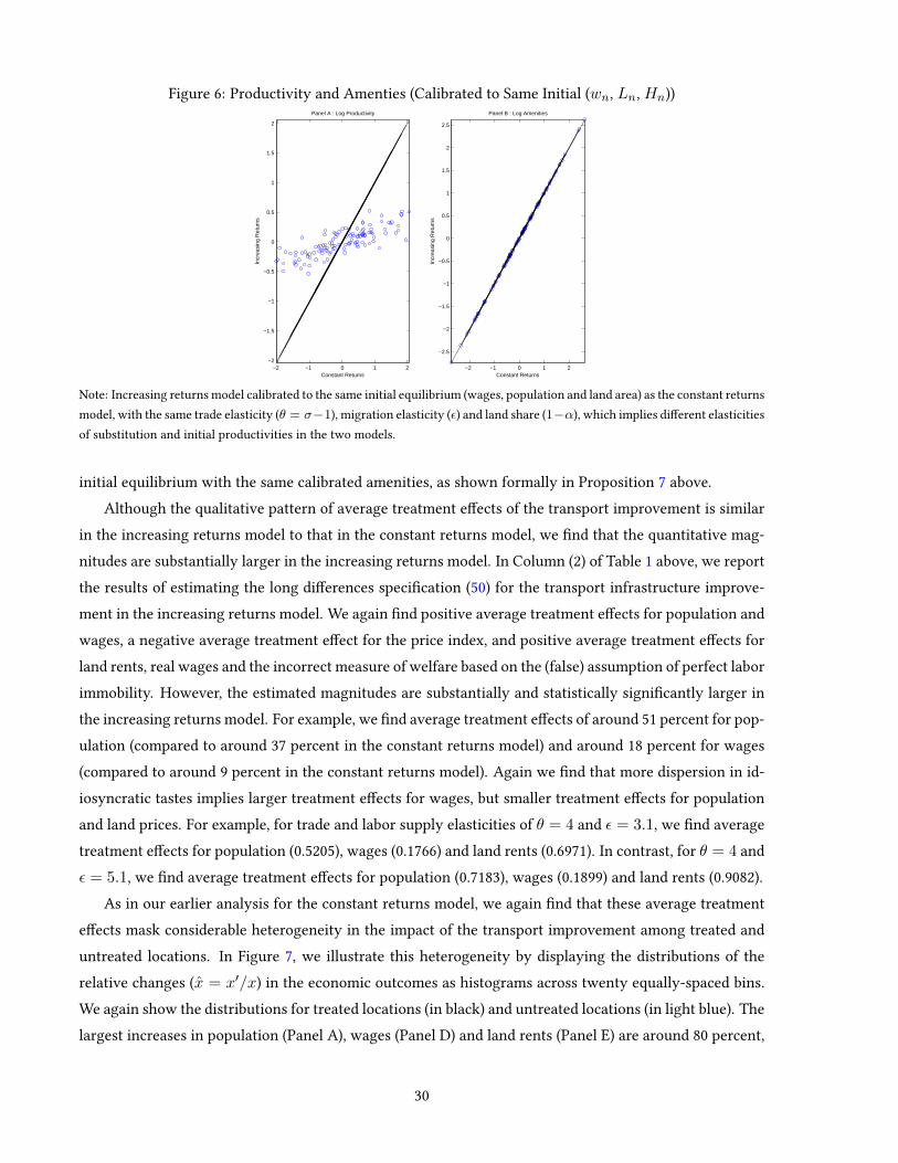
Figure 6: Productivity and Amenties (Calibrated to Same Initial (wn, Ln, Hn))

−2 −1 0 1 2−2

−1.5

−1

−0.5

0

0.5

1

1.5

2

Incr

easi

ng R

etur

ns

Constant Returns

Panel A : Log Productivity

−2 −1 0 1 2

−2.5

−2

−1.5

−1

−0.5

0

0.5

1

1.5

2

2.5

Incr

easi

ng R

etur

ns

Constant Returns

Panel B : Log Amenities

Note: Increasing returns model calibrated to the same initial equilibrium (wages, population and land area) as the constant returnsmodel, with the same trade elasticity (θ = σ−1), migration elasticity (ε) and land share (1−α), which implies dierent elasticitiesof substitution and initial productivities in the two models.

initial equilibrium with the same calibrated amenities, as shown formally in Proposition 7 above.Although the qualitative pattern of average treatment eects of the transport improvement is similar

in the increasing returns model to that in the constant returns model, we nd that the quantitative mag-nitudes are substantially larger in the increasing returns model. In Column (2) of Table 1 above, we reportthe results of estimating the long dierences specication (50) for the transport infrastructure improve-ment in the increasing returns model. We again nd positive average treatment eects for population andwages, a negative average treatment eect for the price index, and positive average treatment eects forland rents, real wages and the incorrect measure of welfare based on the (false) assumption of perfect laborimmobility. However, the estimated magnitudes are substantially and statistically signicantly larger inthe increasing returns model. For example, we nd average treatment eects of around 51 percent for pop-ulation (compared to around 37 percent in the constant returns model) and around 18 percent for wages(compared to around 9 percent in the constant returns model). Again we nd that more dispersion in id-iosyncratic tastes implies larger treatment eects for wages, but smaller treatment eects for populationand land prices. For example, for trade and labor supply elasticities of θ = 4 and ε = 3.1, we nd averagetreatment eects for population (0.5205), wages (0.1766) and land rents (0.6971). In contrast, for θ = 4 andε = 5.1, we nd average treatment eects for population (0.7183), wages (0.1899) and land rents (0.9082).

As in our earlier analysis for the constant returns model, we again nd that these average treatmenteects mask considerable heterogeneity in the impact of the transport improvement among treated anduntreated locations. In Figure 7, we illustrate this heterogeneity by displaying the distributions of therelative changes (x = x′/x) in the economic outcomes as histograms across twenty equally-spaced bins.We again show the distributions for treated locations (in black) and untreated locations (in light blue). Thelargest increases in population (Panel A), wages (Panel D) and land rents (Panel E) are around 80 percent,

30

20 percent and more than 120 percent respectively in the increasing returns model, compared to around 60percent, 10 percent and 70 percent respectively in the constant returns model. We also nd larger increasesin real wages and in the measure of welfare based on the (false) assumption of perfect labor immobility inthe increasing returns model. The magnitudes of the dierences for real wages and immobile welfare aresmaller, which is consistent with our earlier ndings of larger reallocation eects than welfare eects.

Figure 7: Impact of Transport Improvement (Calibrated to Same Initial Equilibrium (wn, Ln, Hn))

0.8 1 1.3 1.6 1.80

0.2

0.4

0.6

Pro

babi

lity

Panel A : Population

1 1.1 1.2 1.3 1.30

0.2

0.4

0.6

Pro

babi

lity

Panel B : Real Wage

0.7 0.7 0.8 0.9 10

0.2

0.4

0.6

Pro

babi

lity

Panel C : Price Index

0.9 1 1.1 1.1 1.20

0.2

0.4

0.6

Pro

babi

lity

Panel D : Wage

0.8 1.1 1.5 1.9 2.20

0.2

0.4

0.6

Pro

babi

lity

Panel E : Land Rents

1 1.1 1.2 1.3 1.40

0.2

0.4

0.6

Pro

babi

lity

Panel F : Incorrect Immobile Welfare

Note: Increasing returns to scale model calibrated to the same initial equilibrium (wages, population and land area) as the constantreturns to scale model, with the same trade elasticity (θN = σG − 1 > σN − 1) and values of other model parameters.

These ndings of larger average treatment eects than in the constant returns model reect the en-dogenous changes in the measures of varieties produced by each location in the increasing returns model.As population increases in treated locations, this expands the measure of varieties produced, which fur-ther increases the attractiveness of these treated locations. In contrast, as population declines in untreatedlocations, this reduces the measure of varieties produced, which further reduces the desirability of theseuntreated locations. As long as the stability condition σ (1− α) > 1 is satised, there is a unique equilib-rium distribution of economic activity across locations, but these agglomeration forces magnify the impactof the transport improvement on the relative attractiveness of locations.

31

5 Regions and Countries

In this section, we explore the implications of a distinction between regions and countries, where work-ers with heterogeneous preferences are mobile across regions within countries, but are immobile acrosscountries (see also Ramondo, Rodríguez-Clare, and Saborio 2012). We show that the general equilibriumof the model can be characterized and counterfactuals can be undertaken using a directly analogous ap-proach to before. We examine the implications of worker mobility across regions within countries for themeasurement of countries’ welfare gains from trade.

5.1 Preferences, Endowments and Technology

We consider a world economy consisting of many (potentially asymmetric) countries indexed by j ∈ J .We allow each country to consist of many (potentially asymmetric) regions indexed by i, n ∈ N j , suchthat the world economy comprises N = N1, . . . , NJ regions. Between countries, labor is completelyimmobile. Within countries, workers have heterogeneous preferences for regions, as modeled in the pre-vious sections. We rst develop this extension of our baseline constant returns model from Section 2, butlater report results for the same extension of our increasing returns model from Section 3.

5.2 General Equilibrium

The general equilibrium of the model again can be represented by the measure of workers (Ln), the tradeshare (πni) and the wage (wn) for each location n, i ∈ N j and each country j ∈ J . Using labor income(13), the trade share (7), the price index (8), residential choice probabilities (10) and land market clearing(14), this equilibrium triple Ln, πni, wn solves the following system of equations for all i, n ∈ N . First,each location’s income must equal expenditure on the goods produced in that location:

wiLi =∑j∈J

∑n∈Nj

πniwnLn. (51)

Second, regional expenditure shares are:

πni =Ai (dniwi)

−θ∑j∈J∑

k∈Nj Ak (dnkwk)−θ . (52)

Third, residential choice probabilities imply:

LnLj

=Bn

(Anπnn

)αεθ(LnHn

)−ε(1−α)∑

k∈Nj Bk

(Akπkk

)αεθ(LkHk

)−ε(1−α) , (53)

where the only dierence is that the residential choice probabilities (Ln/Lj) now apply country by coun-try, so that the summation in the denominator of (53) is across regions k within a given country j.

32

5.3 Counterfactuals

The system of equations for general equilibrium (51)-(53) again provides an approach for undertakingmodel-based counterfactuals that uses only parameters and the values of endogenous variables in an initialequilibrium. Denoting the relative value of variables in the counterfactual and initial equilibria by a hat(x = x′/x), we can solve for the counterfactual eects of a change in trade frictions, productivity oramenities using:

wiλjiYi =

∑m∈J

∑n∈Nm

π′niwnλmn Yn, (54)

πniπni =πniAi

(dniwi

)−θ∑

j∈J∑

k∈Nj πnkAk

(dnkwk

)−θ , (55)

λjnλjn =

BnAαεθn π

−αεθ

nn

(λjn)−ε(1−α)

λjn∑k∈Nj BkA

αεθk π

−αεθ

kk

(λjk

)−ε(1−α)λjk

, (56)

where Yi = wiLi denotes labor income and λjn = Ln/Lj denotes the population share of each location

n ∈ N j within country j in the initial equilibrium. Again the only dierence from before is that theresidential choice probabilities (λjn = Ln/L

j) apply country by country, so that the summation in thedenominator of (56) is across regions k within a given country j.

5.4 Welfare Gains from Trade

As in the specication of the model without the distinction between regions and countries (section 2.9),the common welfare gains from trade across all locations within country j ∈ J can be expressed as aweighted average of the changes in the domestic trade share and population in all locations:

U jT

U jA=

∑n∈Nj

LnL

(πAnnπTnn

)αεθ(LAnLTn

)ε(1−α) 1ε

, (57)

where the summation is now only across locations within country j; these welfare gains in general dieracross countries m 6= j; and πAnn 6= 1 because there is trade across regions within a country even whenthere is no trade between countries under autarky. Equivalently, these common welfare gains from tradewithin country j can be expressed in terms of the change in the domestic trade share (πnn) and population(Ln) of any one location n ∈ N j , and hence in terms of the change in the geometric mean domestic tradeshare (πnn) and geometric mean population (Ln) across locations n ∈ N j :

U jT

U jA=

(πAnnπTnn

)αθ(LAnLTn

) 1ε+(1−α)

=

(πAnnπTnn

)αθ

(LAnLTn

) 1ε+(1−α)

, (58)

where the tilde above a variable denotes a geometric mean across locations within each country, such thatLAn =

[∏n∈Nj LAn

] 1

|Nj | for n ∈ N j .

33

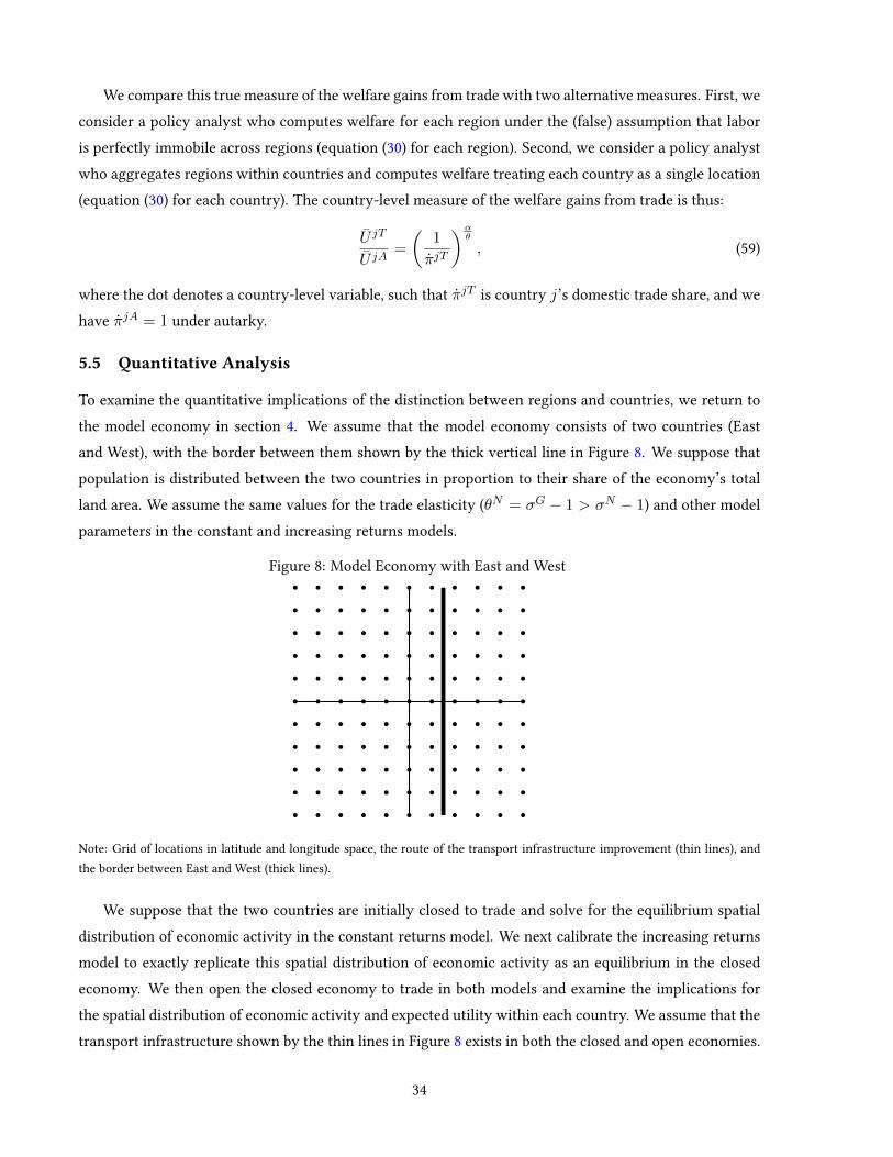
We compare this true measure of the welfare gains from trade with two alternative measures. First, weconsider a policy analyst who computes welfare for each region under the (false) assumption that laboris perfectly immobile across regions (equation (30) for each region). Second, we consider a policy analystwho aggregates regions within countries and computes welfare treating each country as a single location(equation (30) for each country). The country-level measure of the welfare gains from trade is thus:

U jT

U jA=

(1

πjT

)αθ

, (59)

where the dot denotes a country-level variable, such that πjT is country j’s domestic trade share, and wehave πjA = 1 under autarky.

5.5 Quantitative Analysis

To examine the quantitative implications of the distinction between regions and countries, we return tothe model economy in section 4. We assume that the model economy consists of two countries (Eastand West), with the border between them shown by the thick vertical line in Figure 8. We suppose thatpopulation is distributed between the two countries in proportion to their share of the economy’s totalland area. We assume the same values for the trade elasticity (θN = σG − 1 > σN − 1) and other modelparameters in the constant and increasing returns models.

Figure 8: Model Economy with East and West

rrrrrrrrrrr

rrrrrrrrrrr

rrrrrrrrrrr

rrrrrrrrrrr

rrrrrrrrrrr

rrrrrrrrrrr

rrrrrrrrrrr

rrrrrrrrrrr

rrrrrrrrrrr

rrrrrrrrrrr

rrrrrrrrrrr

Note: Grid of locations in latitude and longitude space, the route of the transport infrastructure improvement (thin lines), andthe border between East and West (thick lines).

We suppose that the two countries are initially closed to trade and solve for the equilibrium spatialdistribution of economic activity in the constant returns model. We next calibrate the increasing returnsmodel to exactly replicate this spatial distribution of economic activity as an equilibrium in the closedeconomy. We then open the closed economy to trade in both models and examine the implications forthe spatial distribution of economic activity and expected utility within each country. We assume that thetransport infrastructure shown by the thin lines in Figure 8 exists in both the closed and open economies.

34

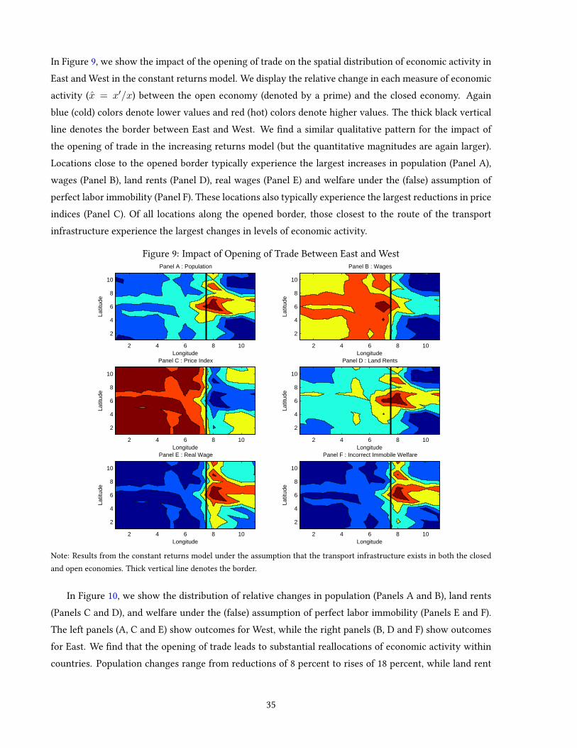
In Figure 9, we show the impact of the opening of trade on the spatial distribution of economic activity inEast and West in the constant returns model. We display the relative change in each measure of economicactivity (x = x′/x) between the open economy (denoted by a prime) and the closed economy. Againblue (cold) colors denote lower values and red (hot) colors denote higher values. The thick black verticalline denotes the border between East and West. We nd a similar qualitative pattern for the impact ofthe opening of trade in the increasing returns model (but the quantitative magnitudes are again larger).Locations close to the opened border typically experience the largest increases in population (Panel A),wages (Panel B), land rents (Panel D), real wages (Panel E) and welfare under the (false) assumption ofperfect labor immobility (Panel F). These locations also typically experience the largest reductions in priceindices (Panel C). Of all locations along the opened border, those closest to the route of the transportinfrastructure experience the largest changes in levels of economic activity.

Figure 9: Impact of Opening of Trade Between East and West

Longitude

Latit

ude

Panel A : Population

2 4 6 8 10

2

4

6

8

10

Longitude

Latit

ude

Panel B : Wages

2 4 6 8 10

2

4

6

8

10

Longitude

Latit

ude

Panel C : Price Index

2 4 6 8 10

2

4

6

8

10

Longitude

Latit

ude

Panel D : Land Rents

2 4 6 8 10

2

4

6

8

10

Longitude

Latit

ude

Panel E : Real Wage

2 4 6 8 10

2

4

6

8

10

Longitude

Latit

ude

Panel F : Incorrect Immobile Welfare

2 4 6 8 10

2

4

6

8

10

Note: Results from the constant returns model under the assumption that the transport infrastructure exists in both the closedand open economies. Thick vertical line denotes the border.

In Figure 10, we show the distribution of relative changes in population (Panels A and B), land rents(Panels C and D), and welfare under the (false) assumption of perfect labor immobility (Panels E and F).The left panels (A, C and E) show outcomes for West, while the right panels (B, D and F) show outcomesfor East. We nd that the opening of trade leads to substantial reallocations of economic activity withincountries. Population changes range from reductions of 8 percent to rises of 18 percent, while land rent

35

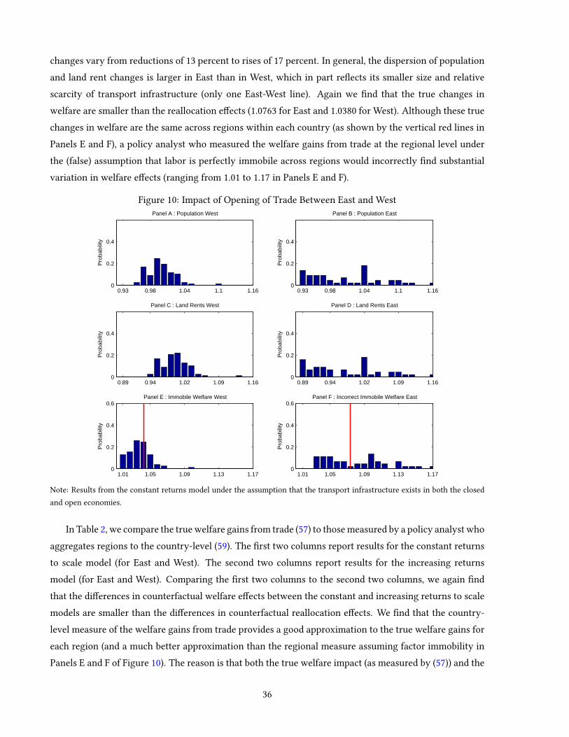
changes vary from reductions of 13 percent to rises of 17 percent. In general, the dispersion of populationand land rent changes is larger in East than in West, which in part reects its smaller size and relativescarcity of transport infrastructure (only one East-West line). Again we nd that the true changes inwelfare are smaller than the reallocation eects (1.0763 for East and 1.0380 for West). Although these truechanges in welfare are the same across regions within each country (as shown by the vertical red lines inPanels E and F), a policy analyst who measured the welfare gains from trade at the regional level underthe (false) assumption that labor is perfectly immobile across regions would incorrectly nd substantialvariation in welfare eects (ranging from 1.01 to 1.17 in Panels E and F).

Figure 10: Impact of Opening of Trade Between East and West

0.93 0.98 1.04 1.1 1.160

0.2

0.4

Pro

babi

lity

Panel A : Population West

0.93 0.98 1.04 1.1 1.160

0.2

0.4

Pro

babi

lity

Panel B : Population East

0.89 0.94 1.02 1.09 1.160

0.2

0.4

Pro

babi

lity

Panel C : Land Rents West

0.89 0.94 1.02 1.09 1.160

0.2

0.4

Pro

babi

lity

Panel D : Land Rents East

1.01 1.05 1.09 1.13 1.170

0.2

0.4

0.6

Pro

babi

lity

Panel E : Immobile Welfare West

1.01 1.05 1.09 1.13 1.170

0.2

0.4

0.6

Pro

babi

lity

Panel F : Incorrect Immobile Welfare East

Note: Results from the constant returns model under the assumption that the transport infrastructure exists in both the closedand open economies.

In Table 2, we compare the true welfare gains from trade (57) to those measured by a policy analyst whoaggregates regions to the country-level (59). The rst two columns report results for the constant returnsto scale model (for East and West). The second two columns report results for the increasing returnsmodel (for East and West). Comparing the rst two columns to the second two columns, we again ndthat the dierences in counterfactual welfare eects between the constant and increasing returns to scalemodels are smaller than the dierences in counterfactual reallocation eects. We nd that the country-level measure of the welfare gains from trade provides a good approximation to the true welfare gains foreach region (and a much better approximation than the regional measure assuming factor immobility inPanels E and F of Figure 10). The reason is that both the true welfare impact (as measured by (57)) and the

36

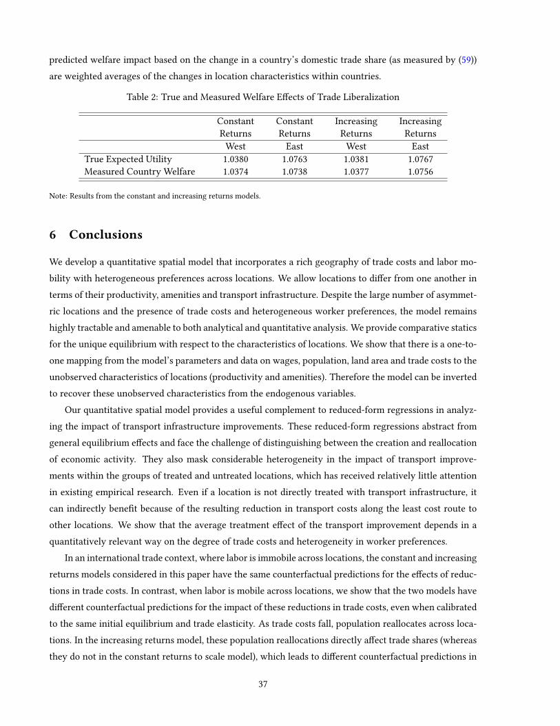
predicted welfare impact based on the change in a country’s domestic trade share (as measured by (59))are weighted averages of the changes in location characteristics within countries.

Table 2: True and Measured Welfare Eects of Trade Liberalization

Constant Constant Increasing IncreasingReturns Returns Returns Returns

West East West EastTrue Expected Utility 1.0380 1.0763 1.0381 1.0767Measured Country Welfare 1.0374 1.0738 1.0377 1.0756

Note: Results from the constant and increasing returns models.

6 Conclusions

We develop a quantitative spatial model that incorporates a rich geography of trade costs and labor mo-bility with heterogeneous preferences across locations. We allow locations to dier from one another interms of their productivity, amenities and transport infrastructure. Despite the large number of asymmet-ric locations and the presence of trade costs and heterogeneous worker preferences, the model remainshighly tractable and amenable to both analytical and quantitative analysis. We provide comparative staticsfor the unique equilibrium with respect to the characteristics of locations. We show that there is a one-to-one mapping from the model’s parameters and data on wages, population, land area and trade costs to theunobserved characteristics of locations (productivity and amenities). Therefore the model can be invertedto recover these unobserved characteristics from the endogenous variables.

Our quantitative spatial model provides a useful complement to reduced-form regressions in analyz-ing the impact of transport infrastructure improvements. These reduced-form regressions abstract fromgeneral equilibrium eects and face the challenge of distinguishing between the creation and reallocationof economic activity. They also mask considerable heterogeneity in the impact of transport improve-ments within the groups of treated and untreated locations, which has received relatively little attentionin existing empirical research. Even if a location is not directly treated with transport infrastructure, itcan indirectly benet because of the resulting reduction in transport costs along the least cost route toother locations. We show that the average treatment eect of the transport improvement depends in aquantitatively relevant way on the degree of trade costs and heterogeneity in worker preferences.

In an international trade context, where labor is immobile across locations, the constant and increasingreturns models considered in this paper have the same counterfactual predictions for the eects of reduc-tions in trade costs. In contrast, when labor is mobile across locations, we show that the two models havedierent counterfactual predictions for the impact of these reductions in trade costs, even when calibratedto the same initial equilibrium and trade elasticity. As trade costs fall, population reallocates across loca-tions. In the increasing returns model, these population reallocations directly aect trade shares (whereasthey do not in the constant returns to scale model), which leads to dierent counterfactual predictions in

37

the two models for wages, trade shares, populations and welfare. We show that these dierences in coun-terfactual predictions can be quantitatively relevant for empirically plausible reductions in trade costs.

We show that reallocations of economic activity across locations play an important role in under-standing the welfare gains from trade. To the extent that some locations experience larger reductions intrade costs than others, populations reallocates to these locations, until the price of land adjusts such thatall locations experience the same welfare gains from trade. We nd that these reallocations of economicactivity are large relative to the overall welfare gains from trade. Failing to take them into account whenmeasuring welfare at the regional level can lead to large discrepancies from the true welfare gains fromtrade. In contrast, measuring the welfare gains from trade at the country-level provides a much closerapproximation to the common welfare gains from trade across regions within each country.

38

References

Allen, T., andC. Arkolakis (2014): “Trade and the Topography of the Spatial Economy,” Quarterly Journalof Economics, forthcoming.

Alvarez, F., and R. E. Lucas (2007): “General Equilibrium Analysis of the Eaton-Kortum Model of Inter-national Trade,” Journal of Monetary Economics, 54, 1726–1768.

Arkolakis, C., A. Costinot, and A. Rodriguez-Clare (2012): “New Trade Models, Same Old Gains,”American Economic Review, 102(1), 94–130.

Artuc, E., S. Chaudhuri, and J. McLaren (2010): “Trade Shocks and Labor Adjustment: A StructuralEmpirical Approach,” American Economic Review, 100(3), 1008–1045.

Baum-Snow, N. (2007): “Did Highways Cause Suburbanization?,” Quarterly Journal of Economics, 122(2),775–780.

Behrens, K., C. Gaigné, G. I. Ottaviano, and J.-F. Thisse (2007): “Countries, Regions and Trade: On theWelfare Impacts of Economic Integration,” European Economic Review, 51, 1277–1301.

Bernard, A. B., J. Eaton, J. B. Jensen, and S. S. Kortum (2003): “Plants and Productivity in InternationalTrade,” American Economic Review, 93(4), 1268–1290.

Blanchard, O., and L. Katz (1992): “Regional Evolutions,” Brookings Papers on Economic Activity, 23(1),1–76.

Bound, J., andH. J. Holzer (2000): “Demand Shifts, Population Adjustments and Labor Market OutcomesDuring the 1980s,” Journal of Labor Economics, 18(1), 20–54.

Bryan, G., andM. Morten (2014): “Economic Development and the Spatial Allocation of Labor: Evidencefrom Indonesia,” Stanford University, mimeograph.

Busso, M., J. Gregory, and P. Kline (2013): “Assessing the Incidence and Eciency of a Prominent PlaceBased Policy,” American Economic Review, 103(2), 897–947.

Caliendo, L., and F. Parro (2012): “Estimates of the Trade and Welfare Eects of NAFTA,” NBER Working

Paper, 18508.

Caliendo, L., F. Parro, E. Rossi-Hansberg, and P.-D. Sarte (2014): “The Impact of Regional and SectoralProductivity Changes on the U.S. Economy,” NBER Working Paper.

Coşar, K., and P. Fajgelbaum (2013): “Internal Geography, International Trade, and Regional Specializa-tion,” NBER Working Paper, 19697.

39

Costinot, A., D. Donaldson, and I. Komunjer (2012): “What Goods Do Countries Trade? A QuantitativeExploration of Ricardo’s Ideas,” Review of Economic Studies, 79(2), 581–608.

Courant, P. N., and A. V. Deardorff (1992): “International Trade with Lumpy Countries,” Journal of

Political Economy, 100(1), 198–210.

(1993): “Amenities, Nontraded Goods, and the Trade of Lumpy Countries,” Journal of Urban Eco-

nomics, 34(2), 299–317.

Davis, D. R., and D. E. Weinstein (2002): “Bones, Bombs, and Break Points: The Geography of EconomicActivity,” American Economic Review, 92(5), 1269–1289.

Davis, M. A., and F. Ortalo-Magné (2011): “Housing Expenditures, Wages, Rents,” Review of Economic

Dynamics, 14(2), 248–261.

Dekle, R., J. Eaton, and S. Kortum (2007): “Unbalanced Trade,” American Economic Review, 97(2), 351–355.

Desmet, K., D. K. Nagy, and E. Rossi-Hansberg (2014): “The Geography of Development: EvaluatingMigration Restrictions and Coastal Flooding,” Princeton University, mimeograph.

Desmet, K., and E. Rossi-Hansberg (2014): “Spatial Development,” American Economic Review, forthcom-ing.

Donaldson, D. (2014): “Railroads of the Raj: Estimating the Impact of Transportation Infrastructure,”American Economic Review, forthcoming.

Donaldson, D., and R. Hornbeck (2016): “Railroads and American Economic Growth: A “Market Access”Approach,” Quarterly Journal of Economics, forthcoming.

Duranton, G., andM. A. Turner (2012): “Urban Growth and Transportation,” Review of Economic Studies,79(4), 1407–1440.

Eaton, J., and S. Kortum (2002): “Technology, Geography, and Trade,” Econometrica, 70(5), 1741–1779.

Eaton, J., S. Kortum, B. Neiman, and J. Romalis (2011): “Trade and the Global Recession,” NBER Working

Paper, 16666.

Faber, B. (2014): “Integration and the Periphery: The Unintended Eects of New Highways in a Develop-ing Country,” Review of Economic Studies, forthcoming.

Fieler, C. (2011): “Non-Homotheticity and Bilateral Trade: Evidence and a Quantitative Explanation,”Econometrica, 79(4), 1069–1101.

Fogel, R. (1964): Railroads and American economic growth: Essays in econometric history. Johns HopkinsUniversity Press, Baltimore (md).

40

Fujita, M., P. Krugman, and A. J. Venables (1999): The Spatial Economy: Cities, Regions and International

Trade. MIT Press, Cambridge.

Grogger, J., and G. Hanson (2011): “Income Maximization and the Selection and Sorting of InternationalMigrants,” Journal of Development Economics, 95(1), 42–57.

Hanson, G. H. (1996): “Localization Economies, Vertical Organization, and Trade,” American Economic

Review, 86(5), 1266–1278.

(1997): “Increasing Returns, Trade, and the Regional Structure of Wages,” Economic Journal, 107(1),113–133.

(2005): “Market Potential, Increasing Returns, and Geographic Concentration,” Journal of Inter-national Economics, 67(1), 1–24.

Head, K., and J. Ries (2001): “Increasing Returns versus National Product Dierentiation as an Explanationfor the Pattern of U.S.-Canada Trade,” American Economic Review, 91, 858–876.

Helpman, E. (1998): “The Size of Regions,” in Topics in Public Economics: Theoretical and Applied Analysis,ed. by D. Pines, E. Sadka, and I. Zilcha. Cambridge University Press, Cambridge.

Hsieh, C.-T., and R. Ossa (2011): “A Global View of Productivity Growth in China,” NBER Working Paper,16778.

Jones, R. (1967): “International Capital Movements and the Theory of Taris and Trade,” Quarterly Journalof Economics, 81, 1–38.

Kennan, J., and J. R. Walker (2011): “The Eect of Expected Income on Individual Migration Decisions,”Econometrica, 79(1), 211–251.

Krugman, P. (1991a): Geography and Trade. MIT Press, Cambridge.

(1991b): “Increasing Returns and Economic Geography,” Journal of Political Economy, 99(3), 483–499.

Krugman, P., and A. J. Venables (1995): “Globalisation and Inequality of Nations,” Quarterly Journal of

Economics, 60, 857–80.

Markusen, J. R. (1983): “Factor Movements and Commodity Trade as Complements,” Journal of Interna-tional Economics, 14(34), 341–356.

McFadden, D. (1974): “The Measurement of Urban Travel Demand,” Journal of Public Economics, 3(4),303–328.

41

Michaels, G. (2008): “The Eect of Trade on the Demand for Skill: Evidence from the Interstate HighwaySystem,” Review of Economics and Statistics, 90(4), 683–701.

Moretti, E. (2011): “Local Labor Markets,” in Handbook of Labor Economics, ed. by D. Card, and O. Ashen-felter, vol. 4b, pp. 1238–1303. Elsevier North Holland, Amsterdam.

Mundell, R. A. (1957): “International Trade and Factor Mobility,” American Economic Review, 47, 321–337.

Ossa, R. (2011): “Trade Wars and Trade Talks with Data,” NBER Working Paper, 17347.

Puga, D. (1999): “The Rise and Fall of Regional Inequalities,” European Economic Review, 43, 303–334.

Ramondo, N., A. Rodríguez-Clare, andM. Saborio (2012): “Scale Eects and Productivity Across Coun-tries: Does Country Size Matter?,” NBER Working Paper, 18532.

(2016): “Trade, Domestic Frictions, and Scale Eects,” American Economic Review, forthcoming.

Redding, S., and M. Turner (2015): “Transportation Costs and the Spatial Organization of EconomicActivity,” in Handbook of Urban and Regional Economics, ed. by G. Duranton, J. V. Henderson, and

W. Strange, vol. 5, chap. 20, pp. 1339–1398. Elsevier: North Holland, Amsterdam.

Redding, S. J. (2012): “Goods Trade, Factor Mobility and Welfare,” NBER Working Paper, 18008.

Redding, S. J., and D. M. Sturm (2008): “The Costs of Remoteness: Evidence from German Division andReunication,” American Economic Review, 98(5), 1766–1797.

Redding, S. J., and A. J. Venables (2004): “Economic Geography and International Inequality,” Journal ofInternational Economics, 62(1), 53–82.

Rossi-Hansberg, E. (2005): “A Spatial Theory of Trade,” American Economic Review, 95(5), 1464–1491.

Simonovska, I., and M. E. Waugh (2014): “The Elasticity of Trade: Estimates and Evidence,” Journal of

International Economics, 92(1), 34–50.

42