Government intervention and information aggregation

by prices1

Philip Bond2 Itay Goldstein3

September 30, 2014

1We thank Campbell Harvey (the editor), an anonymous referee and associate editor, alongViral Acharya, Michael Fishman, William Fuchs, Qi Liu, Adriano Rampini, Jean-Charles Rochet,Duane Seppi, and seminar audiences at the Bank of Israel, Dartmouth College, the Federal ReserveBanks of Chicago, Minneapolis and New York, the International Monetary Fund, MIT, MichiganState University, New York University, the University of California at Berkeley, the University ofCalifornia at Irvine, the University of Delaware, the University of Illinois at Chicago, the Univer-sity of Maryland, the University of North Carolina at Chapel Hill, the University of Waterloo,the University of Wisconsin, Washington University in St Louis, York University, the 2009 Finan-cial Crisis Workshop at Wharton, the 2010 American Economic Association meetings, the 2010FIRS Conference, the 2010 NBER Summer Institute on Capital Markets and the Economy, the2010 Chicago-Minnesota Accounting Theory Conference, the third Theory Workshop on Corpo-rate Finance and Financial Markets at Boston University, the 2011 American Finance Associationmeetings, the 2012 NY Fed- NYU Financial Intermediation Conference, the 2012 University ofWashington Summer Finance conference, the 2012 Society for Economic Dynamics conference, andthe 2013 IDC Summer Workshop for helpful comments. Bond thanks the Cynthia and BennettGolub Endowed Faculty Scholar Award Fund for financial support. All errors are our own.

2University of Washington.3University of Pennsylvania.

Abstract

Governments intervene in firms’ lives in a variety of ways. However, efficient intervention

depends on various economic variables, about which governments often have only limited

information. Consequently, many researchers and policymakers call for governments to at

least partially “follow the market” and make intervention decisions based on the information

revealed by stock market prices. We analyze the implications of governments’ reliance on

market information for market prices and government decisions, and show that the use of

market information might not come for free. A key point is that price informativeness is

endogenous to government policy. In some cases, it is optimal for a government to marginally

reduce its reliance on market prices in order to avoid harming traders’ incentives to trade

and the concomitant aggregation of information into market prices. For similar reasons, it

is optimal for a government to limit transparency in some dimensions.

Our paper is motivated by two key observations. First, governments play an important

role in the lives of firms and financial institutions, and take actions that have significant

implications for their cash flows and stock prices. Second, governments’ actions often follow

financial market movements; and, closely related, many government officials view market

prices as a useful source of information, and a number of policy proposals advocate making

more explicit use of this information.

In this paper we analyze the implications of a government’s use of market information in

light of a key economic force: market prices reflect not only the fundamentals about which a

government may wish to learn, but also expected government actions. Consequently, when

governments make decisions based on information they glean from market prices, this affects

the amount of information the government can ultimately extract from the market. We first

analyze the equilibrium effect of these forces, and derive cross-sectional implications. Second,

we analyze whether a government should increase or decrease its reliance on the market.

Third, we develop implications for other issues—in particular, whether a government should

reveal its own information to the market (i.e., transparency).

Before detailing our findings, we expand upon our opening two observations. The first

observation is well-illustrated by the course of the recent financial crisis, during which gov-

ernment bailouts of leading financial institutions (e.g., AIG and Citigroup) and other firms

(such as in the auto industry) constituted very important events for these firms and insti-

tutions. Government actions remain important following the crisis, as exemplified by recent

penalties and regulations for financial institutions.

These government actions—and especially transfers made during the crisis—have at-

tracted much controversy, both in policy and academic circles. Critics of government trans-

fers argue that they waste taxpayer funds; unfairly reward both bankers and their share-

holders; and engender future moral hazard. On the other side, proponents of government

transfers argue that they help to soften the negative externalities that would flow from weak

bank balance sheets, notably reduced lending and financial contagion.1

1

Regardless of the balance between the costs and benefits of government intervention,

however, there is little debate that it is desirable that a government be in a position to make

an informed decision. The concern is that the government conducts major interventions

without having very precise information about the fundamentals, costs, and benefits.2 For

example, prior to the collapse of Lehman Brothers, the US government had to quickly decide

whether or not to bail out Lehman. Ideally, this decision requires information about the state

of Lehman, the implications of its failure for the financial system, and the potential moral

hazard that a bailout might create for future episodes. Obtaining and analyzing all this

information in a short amount of time is impossible.

This concern leads to the second key observation mentioned above. The challenge of

making intervention decisions under limited information is well-understood by policymakers

themselves, and one oft-proposed solution is to learn from and base intervention decisions on

market prices. Indeed, a basic tenet of financial economics is that market prices aggregate

information from many different market participants (Hayek 1945; Grossman 1976; Roll

1984). As such, market prices can provide valuable guidance. As an illustration, consider

the following excerpt from a 2004 speech of Ben Bernanke:

Central bankers naturally pay close attention to interest rates and asset prices, in

large part because these variables are the principal conduits through which mon-

etary policy affects real activity and inflation. But policymakers watch financial

markets carefully for another reason, which is that asset prices and yields are

potentially valuable sources of timely information about economic and financial

conditions. Because the future returns on most financial assets depend sensitively

on economic conditions, asset prices–if determined in sufficiently liquid markets–

should embody a great deal of investors’ collective information and beliefs about

the future course of the economy.

Other senior Federal Reserve officials—for example, Minneapolis Federal Reserve Bank

presidents Gary Stern and Narayana Kocherlakota—have voiced similar opinions.

2

Inspection of government actions in the recent crisis indeed suggests that policymakers

watch prices closely, and often use price movements to justify their actions. For example, the

2011 report of the Special Inspector General for the Troubled Asset Relief Program states

that “short sellers were attacking [Citigroup] ... Citigroup’s share price fell from around

$13.99 at the markets close on November 3, 2008, to $3.05 per share on November 21, 2008,

before closing that day at $3.77. In the week leading up to the decision to extend Citigroup

extraordinary assistance, Citigroup’s stock decreased far more than that of its peers.” Beyond

anecdotal evidence, empirical studies from before the crisis establish that government actions

are significantly affected by market prices.3

In addition to existing government responses to financial markets, a range of policy

proposals call for governments to make (more) use of market prices, particularly in the

realm of bank supervision (e.g., Evanoff and Wall (2004) and Herring (2004)). Such policy

proposals are increasingly prominent in the wake of the recent crisis and the perceived failure

of financial regulation prior to it (e.g., Hart and Zingales (2011).)

In light of these observations, in this paper we study a model of information aggregation

in financial markets, where information aggregated in the price is used by the government to

make an intervention decision. A central implication is that relying on market information

is not as simple as the public discussion mentioned above seems to suggest and may not so

easily solve the problem of the government being uninformed. The problem stems from the

fact that prices of financial securities—from which the government attempts to learn—are

not pure projections of the state variables that the government wishes to learn about. Rather,

prices are projections of future cash flows, which are typically affected by government actions.

The information in security prices is thus endogenous and is affected by government policies,

and to the extent that governments rely on prices. When governments rely on market prices,

it is thus important to consider the consequences this has for price informativeness.

For illustration, consider the case of a government bailout or a guarantee for a financial

institution. Empirical evidence clearly shows such actions benefit the institution’s sharehold-

3

ers, and are reflected in increased share prices. For example, O’Hara and Shaw (1990) show

that an increase in expectations that a government will provide a guarantee to large financial

institutions is immediately reflected in share price increases for such institutions. Gandhi

and Lustig (2013) show that shares of large financial institutions are priced at a premium,

reflecting the benefit that their shareholders expect from government intervention. Hence,

government actions affect prices, and consequently also affect the ability of the government

to learn from prices. This affects the desirability of market-based intervention.

To understand these forces, it is important to consider the process by which prices ag-

gregate information. We analyze how market-based government policy affects speculators’

trading incentives, and hence the extent to which financial markets aggregate dispersed in-

formation. We build on the canonical model of information aggregation of Grossman (1976),

Hellwig (1980), and Admati (1985). Speculators possess heterogenous information about

the payoffs of an asset and trade in a market that is subject to noise/liquidity shocks. The

equilibrium price of the asset then reflects the aggregated information of speculators with

noise. In the existing literature, the asset’s cash flows are exogenous. However, if the

government (or some other decision maker) uses information in prices when intervening in

the firm’s operations in a way that affects the firm’s cash flows, then the cash flows are

instead endogenous and depend on market prices and on the trading process. Our modeling

innovation is to introduce this effect into an analysis of information aggregation.

In the model, the government makes an intervention decision based on market infor-

mation and on other information it has about the firm or the financial institution. Such

information can come from the government’s own supervision activities conducted by the

Federal Reserve Banks, the Federal Deposit Insurance Corporation, etc. The government

uses market signals because they contain information, but their informational content is en-

dogenous and determined by the trading incentives of speculators, which in turn are affected

by the government’s policy and the extent to which it relies on the market price.

We identify two opposing effects of the government’s reliance on stock prices on price in-

4

formativeness. The first effect is the Information Importance Effect. When the government

puts more weight on the price and less weight on its own information in the intervention deci-

sion, it makes speculators’ information, conditional on the price, less important in predicting

the government’s action and hence the value of the security. This reduces speculators’ incen-

tives to trade on their information, and hence it reduces price informativeness. The second

effect is the Residual Risk Effect. When the government puts more weight on the price and

less weight on its own information in the intervention decision, it reduces the uncertainty

that speculators are exposed to when they trade. Being risk averse, speculators then trade

more aggressively on their information, and this leads to an increase in price informativeness.

Overall, which effect dominates depends on the parameters of the model. The residual

risk effect is weakened when the risk for speculators is driven mostly by exogenous risk (i.e.,

risk from an unforecastable and exogenous cash flow shock) rather than by endogenous risk

(i.e., risk due to the unknown government action), and so in this case price informativeness

is decreasing in the extent to which the government relies on market prices. We show that

this effect is strong enough to imply that the government follows the market too much, and,

if possible, would gain from a commitment to marginally underweight market prices in its

intervention decision.4 Overall, our model delivers the somewhat paradoxical result that a

government should marginally reduce its reliance on prices precisely when they are informa-

tive, because in this case prices forecast the government’s action well, and so endogenous

risk is low. Similarly, and again paradoxically, a government should marginally increase its

reliance on prices when its own information is relatively precise.

These results are in contrast to a common theme in the literature. While papers by

Faure-Grimaud (2002), Rochet (2004), Hart and Zingales (2011) and others suggest that gov-

ernments should commit to intervene in a pre-determined way based on publicly observable

prices, our paper highlights another consideration to be taken into account when assessing

the costs and benefits of these proposals: the effect that such proposals have on price infor-

mativeness. In particular, in the circumstances above, commitment to a market-based rule

5

reduces the price-informativeness that the rule makes use of, and hence reduces the rule’s

value. In addition, in such circumstances, our model also implies that the government’s own

information is valuable beyond its direct effect on the efficiency of the government’s decision.

When the government has more precise information, it relies less on the market price, and

this makes the market price more informative. Hence there are complementarities between

the government’s own information and the market’s information, and so it is not advisable

for the government to rely completely on market information.

Another important aspect of government policy is transparency. Should the government

reveal its own information publicly? This issue has been hotly debated recently in relation

to regulatory stress tests of financial institutions. There are various views on whether the

results of such stress tests should be publicly disclosed (see Goldstein and Sapra (2013)

for a survey). Our model sheds light on this debate from a new angle: is disclosure of

information to the market desirable when the government is trying to learn from the market?

In our framework, the answer to this question depends on the type of information being

disclosed. If the government discloses information about a variable about which speculators

have at least some additional information, then the government harms itself because the

disclosed information reduces the incentives of speculators to trade on their information

(due to the information importance effect) and reduces the government’s ability to learn.

If instead the government discloses information about a variable that speculators know less

than the government (i.e., their information is a coarsening of the government’s), it helps

itself, because the disclosed information reduces the risk that speculators face (due to the

residual risk effect), causing them to trade more and increasing the government’s ability to

learn from prices. This distinction is new to the literature on transparency.5 In practice, it

seems likely that individual bank conditions are an area in which speculators have substantial

information not possessed by a government. At the opposite extreme, a government knows

its own policy objectives, so there is no room for speculators to have useful information in this

dimension. Consequently, transparency about policy objectives is useful for the government,

6

but transparency about stress-test findings on individual bank conditions might be harmful.

Our paper adds to a growing literature on the informational feedback from asset prices to

real decisions.6 In particular, it complements papers such as Bernanke and Woodford (1997),

Goldstein and Guembel (2008), Bond, Goldstein and Prescott (2010), Dow, Goldstein and

Guembel (2010), and Lehar, Seppi and Strobl (2010), which analyze distinct mechanisms via

which the use of price information in real decisions might reduce the informational content

of the price. For a recent review of this literature, see Bond, Edmans, and Goldstein (2012).

Relative to these papers, our focus is on the efficiency of aggregation of dispersed information

by market prices. This topic, which has long been central in economics and finance (e.g.,

Hellwig (1980)), has not been analyzed in any of the related papers.

The remainder of the paper is organized as follows. Sections I and II first describe

and then analyze the basic model. Section III analyzes how a government should opti-

mally use market information. Section IV looks at the importance of the government’s own

information. Section V analyzes the costs and benefits of transparency. Section VI consid-

ers alternative notions of price informativeness. Section VII considers varying government

subsidies to security holders. Section VIII concludes. The appendix contains most proofs.

I. The model

We focus on one firm (a financial institution, for example), whose shares trade in a financial

market. At t = 0, speculators obtain private signals about a variable that affects the

government’s incentive to intervene in the firm, and trade on these signals. At t = 1, the

government observes the firm’s share price and an additional private signal, and makes a

decision about its intervention. At t = 2, cash flows are realized and speculators are paid.

7

A. Cash flows and government intervention

The firm’s cash flow is X = δ + T . The component δ is exogenous, and unforecastable:

neither speculators nor the government receive any signal about δ before its realization at

t = 2. The distribution of δ is normal, with mean δ and variance var [δ]. The mean δ̄ can

vary across firms, states of the world, and time, but it is publicly known as of t = 0. The

precision of prior information about δ is τ δ ≡ var [δ]−1.

The component T of the firm’s cash flow is the result of endogenous government interven-

tion. Positive values of T represent cash injections or other interventions that increase the

firm’s cash flow, while negative values represent penalties or interventions that reduce the

firm’s cash flow. As discussed in the introduction, a wide variety of government actions affect

firm cash flows. We adopt a general formulation that accommodates many such examples.

In particular, T is chosen by the government to maximize an objective function of the form

E [v (T − θ)− µT |sG, P ] . (1)

Here, v is a concave function that represents the benefits of intervention; θ is a state variable

that is unobserved by the government but that affects these benefits; and µ is a scalar,

which allows for an additional linear cost of intervention. The unobserved state variable θ is

normally distributed with mean θ and variance var [θ], and is independent of the cash flow

shock δ. The precision of prior information about θ is τ θ ≡ var [θ]−1.

The government makes its intervention decision after observing two pieces of information:

a market price P , discussed in detail below, and a noisy signal sG≡ θ + εG of θ, where the

noise term εG is normally distributed with mean 0 and variance var [εG], and is independent

of θ and δ. The precision of the government’s signal is τG ≡ var [εG]−1.

Let us elaborate on the government’s objective function, before proceeding to discuss the

trading environment in the next subsection. As mentioned above, the specification of the

government’s objective function is general enough to cover a range of possible applications.

8

Many interventions in the recent crisis—such as TARP, TALF, and other related govern-

ment programs—intended to provide resources to banks in the hope of increasing lending

to non-financial firms in a period when government officials believed the credit market was

impaired. Our framework can capture such motives, as follows. Consider the case in which

the firm is a bank, and bank loans generate some social surplus. In particular, let s (x− θ1)

be the marginal social surplus created by the xth dollar loaned. The function s is decreas-

ing, reflecting diminishing marginal social returns to lending, and θ1 is a state variable that

affects the social surplus of bank loans. Absent government intervention, the bank lends its

available resources L + θ2, where L is a publicly observable quantity related to the bank’s

balance sheet, and θ2 is a state variable that determines the bank’s ability to access funds

in external credit markets. The government’s intervention provides additional resources T

to the bank, so that its overall lending changes to L + θ2 + T . Finally, write v for the

anti-derivative of s. Consequently, if the government’s cost of funds is µ, then conditional

on θ1 and θ2 the social surplus associated with an intervention T is:7

ˆ L+θ2+T

0

s (x− θ1) dx− µT = v (L+ T − (θ1 − θ2))− v (−θ1)− µT.

Since L is known and v (−θ1) is outside the government’s control, this is consistent with

the objective function (1), with θ = θ1 − θ2. To summarize, the government is concerned

about the amount of credit banks provide, and sets T to influence it. When choosing T , the

government faces uncertainty about the desirability of bank lending (θ1) and/or the amount

of resources banks can get without government intervention (θ2). (We note that our analysis

requires government uncertainty about only one of θ1 and θ2.)

As noted in the introduction, another oft-invoked rationale for government intervention

in financial institutions is the need to maintain financial-sector stability. The concern is

that the failure of a systemically important financial institution (SIFI) might severely harm

the whole financial system. A possible remedy is for the government to inject capital or

9

provide loan guarantees to troubled institutions. However, such remedies have the cost of

engendering future moral hazard problems, encouraging banks to take excessive risks. Events

in the recent crisis reflect this dilemma. On the one hand, the bailout of Citigroup, Bear

Stearns, AIG, and others, was driven by a concern that due to their systemic importance, the

cost of their failure would be very large. On the other hand, Lehman Brothers was allowed

to fail, probably because of concerns that a bailout would create a severe moral hazard issue.

In our model, v (T − θ) reflects the benefit from injecting capital into a distressed financial

institution, and is concave in the amount injected. The benefit depends on the state variable

θ, which reflects the size of the reduction in negative externalities stemming from reducing

a SIFI’s failure probability, net of the cost of increased moral-hazard. The government does

not have perfect information about the state θ, and may try to glean information from the

stock market (see introduction). Note that the government may choose T to be negative,

corresponding to reducing the size of the financial institution in an effort to promote stability.

While the above motivations involve the financial sector, which is a prime focus of gov-

ernment intervention, our framework also covers non-financial firms. For example, the three

large US automakers also received significant government assistance in the recent crisis, and

the justification for this assistance was again the mitigation of negative externalities associ-

ated with bankruptcy. There was concern that the failure of a large automaker would harm

employees, dealers, and suppliers, in turn harming the aggregate economy. In our framework,

v (T − θ) represents the social benefit from transfers to an automaker, where θ, which the

government is not sure of, represents the size of negative externalities.

In summary, in each of these applications the government intervenes in a firm or financial

institution to try to increase overall efficiency in cases where the firm does not internalize the

externalities it generates. We do not take a stand on the source of externalities, but instead

use a general formulation that encompasses multiple cases, as described above.8 We focus

on the interaction between the government and the financial market when the government

is only partially informed about the state θ that determines its desired level of intervention,

10

while financial market participants possess some information about this state.

B. Trading in the financial market

We now complete the description of the model by describing the financial market and the

price formation process. There is a continuum [0, 1] of speculators, each with constant

absolute risk aversion (CARA) utility, u (c) = −e−αc, where c denotes consumption and α

is the absolute risk aversion coefficient. Speculators trade shares in the firm. The shares

pay out the firm cash flow X. Each speculator i receives a noisy signal si ≡ θ + εi of the

state θ. The noise terms εi are independently and identically distributed across speculators,

and each is normally distributed with mean 0 and variance var [εi]. The precision of each

speculator’s signal is τ ε ≡ var [εi]−1. One interpretation of these private signals is that

different speculators have different assessments of the extent to which a firm affects the rest of

the economy, and the government can benefit from their combined knowledge. For example,

as Bear Stearns and Lehman Brothers approached failure, it was unclear to everyone—

including the government—how much their failures would damage the economy.

Each speculator chooses a trade size xi to maximize his expected utility, conditional on

the information in his private signal si and the (endogenously determined) share price P :

xi (si, P ) = arg maxx̃

E[−e−αx̃(δ+T−P )|si, P

]. (2)

Here, if a speculator trades xi, his overall wealth is xi (δ + T − P ), where δ + T is the cash

flow from the security after intervention, and P is the price paid for it.

In addition to informed trading by speculators, there is a noisy supply shock, −Z, which

is normally distributed with mean 0 and variance var [Z]. We again use the notation

τ z ≡ var [Z]−1. Finally, the market-clearing condition is

ˆxi (si, P ) di = −Z. (3)

11

C. Remarks

We conclude this section by briefly highlighting and discussing the assumptions in our frame-

work:

Remark 1: The restriction that the benefit function v is concave is standard, mild, and

likely to be satisfied by many potential applications. The stronger assumptions imposed

on the government’s objective are that (a) the intervention T and state variable θ enter v

linearly, and (b) the cost of intervention is linear, i.e., µT , rather than strictly convex. With

respect to (a), we note that this property arises naturally when T and θ have the same

units. The application to impaired credit markets illustrates this well in the case in which

government uncertainty is about θ2: both T and θ2 are resources on the bank’s balance

sheet, and so are directly comparable. In other cases, such as this same application when

government uncertainty is about the social value of lending θ1, (a) is better viewed as an

approximation made to obtain analytic tractability. With respect to (b), we note first that

linearity of the cost of intervention is the appropriate assumption when the intervention

is small relative to the economy. This is the case for most single-institution interventions.

Second, our framework also covers cases in which the benefit of intervention is linear, but

the government is unsure of the cost, which takes a convex form −v (T − θ). That said, for

extremely large government interventions (the Irish bank bailout may be a good example),

the government’s objective may be best modeled as v (T − θ)−µ (T ), where µ (·) is a convex

cost function, i.e., concave benefit and convex cost.9 For these cases, analytic tractability

requires stronger assumptions on the form of the functions v and µ: for example, if v takes

the same form as speculator preferences, namely constant absolute risk aversion, and µ is

likewise an exponential function, then these cases also fall within our framework: see Lemma

1 below.

Remark 2: A key ingredient in our analysis is that the intervention T affects the value

of the traded security. The fact that T affects the cash flow one-for-one, i.e., X = δ + T , is

unimportant and is assumed here only for simplicity. Section VII analyzes an extension in

12

which a fraction of the injection T is taxed away, so that security holders do not benefit from

the full injection. As discussed in the introduction, there is ample evidence that government

interventions affect security values. For example, both O’Hara and Shaw (1990) and Gandhi

and Lustig (2013) provide evidence that financial institutions’ share prices reflect expecta-

tions of government bailouts. We do not take a stand on why governments do not design

interventions to avoid windfall gains for shareholders,10 but instead take this feature from

the data and analyze the interaction between government intervention and market prices.

Remark 3: The main effects in our model all stem from the fact that speculators try to

forecast government actions, and these forecasts affect market prices and their informative-

ness. As discussed in the introduction, we think this is important for many firms. To focus

our analysis on this effect, in our model the only information speculators have is about a

state variable, θ, that affects government actions. However, a prior draft of the paper (avail-

able on request) analyzes a variant of our model in which speculators also have information

that is directly relevant for the cash flows of the firm even absent government intervention.

II. Equilibrium outcomes

In equilibrium, individual speculators’ demands maximize utility given si and P (i.e., (2)

holds), the market clearing condition (3) holds, and the government’s choice of T maximizes

its objective (1) given its signal sG and the price P . As is standard in almost all the literature,

we focus on linear equilibria in which the price P is a linear function of the average signal

realization—which equals the realization of the state θ—and the supply shock −Z. The

complication in our model relative to the existing literature is that the firm’s cash flow is

affected by the government’s endogenous intervention T . Nonetheless, and as we next show,

there is an equilibrium in which not only is price a linear function of the primitive random

variables, but the intervention T is also linear in these same primitive random variables.

Let us conjecture that in equilibrium T is indeed a linear function of the primitive random

13

variables. In the proof of Proposition 1 below, we show (by largely standard arguments)

that this leads to a linear price function. Then, given that the government learns from

the price P and its own signal sG, and given that all primitive random variables in the

model are normally distributed, the conditional distribution of θ given the government’s

information (P, sG) is also normal.11 Consequently, we can apply the following useful result,

which confirms our conjecture that T is a linear function.

Lemma 1: If the conditional distribution of the state variable θ given government information

(P, sG) is normal, then there exists a function g such that the intervention T that maximizes

the government’s objective (1) is12

T = E [θ|P, sG] + g (µ, var [θ|P, sG]) . (4)

The proof of Lemma 1 is short, and we give it here. The intervention T that maximizes

the government’s objective (1) satisfies the first-order condition

E [v′ (T − θ) |P, sG] = µ. (5)

The government knows T , and so, by hypothesis, the conditional distribution of T − θ given

(P, sG) is normal; consequently, it is fully characterized by its first two moments. Hence,

the expectation E [v′ (T − θ) |P, sG] can be written as a function of the first two moments of

the conditional distribution of T − θ, i.e., there exists some function G : <2 → < such that

E [v′ (T − θ) |P, sG] = G (E [T − θ|P, sG] , var [T − θ|P, sG]) . (6)

Substituting (6) into (5) and defining the inverse g (y, x) of G by G (g (y, x) , x) = y delivers13

T − E [θ|P, sG] = g (µ, var [θ|P, sG]) ,

14

completing the proof of Lemma 1.

Proposition 1 below uses Lemma 1 to establish the existence of a linear equilibrium, and

to characterize the associated level of price informativeness. Before stating the formal result,

we give an informal derivation of price informativeness.

In a linear equilibrium, the price can be written as

P = p0 + pZ (ρθ + Z) , (7)

for some (endogenous) scalars p0, pZ and ρ. Here, ρ2τZ measures price informativeness, since

the informational content of the price is the same as the linear transformation 1ρpZ

(P − p0) =

θ + ρ−1Z, which is an unbiased estimate of the state θ with precision ρ2τZ . Intuitively, the

price of the security is affected by both changes in the state θ and changes in the noise

variable Z; price informativeness is greater when ρ, the ratio of the effect of θ on the price

relative to the effect of Z on the price, is greater. Because we typically take τZ as fixed

in our comparative statics and policy analysis, we often refer to ρ, which is affected by the

underlying parameters and government policy, as price informativeness.

It is worth highlighting that the informativeness measure ρ relates to the state θ, and

not the cash flow T + δ. This is because the government is attempting to learn the state θ

from the price, and so informativeness about θ is the relevant object for the government’s

maximization problem. We discuss this distinction in more detail in Section VI below.

To characterize price informativeness, we first analyze the government’s decision. Given

normality of the state θ, the supply shock −Z, and the error term εG in the government’s

signal sG, along with the linear form of the price function (7), the government’s posterior of

the state θ is normal, with the posterior mean taking the linear form

E [θ|sG, P ] = w (ρ) sG +KP (ρ)1

ρpZ(P − p0) +Kθ (ρ) θ̄, (8)

where Kθ (ρ), KP (ρ) and w (ρ) are weights that sum to one and are derived by standard

15

Bayesian updating, i.e.,

KP (ρ) ≡ ρ2τ zτ θ + ρ2τ z + τG

(9)

w (ρ) ≡ τGτ θ + ρ2τ z + τG

. (10)

In particular, w (ρ) is the weight the government puts on its own signal in estimating the

state, which depends on the information available in the price. As one would expect, the

government puts more weight on its own signal when it is precise (τG high) and less when

the price is informative (ρ and/or τZ high). Given the policy rule (4), the intervention is

T (sG, P ) = w (ρ) sG +KP (ρ)1

ρpZ(P − p0) +Kθ (ρ) θ̄ + g (µ, var [θ|P, sG]) . (11)

Turning to the speculators, each speculator assigns a normal posterior (conditional on

his own signal si and price P ) to the state θ. Then, from (11), each speculator also assigns

a normal posterior to the intervention T . Consequently, applying the well known expression

for a CARA individual’s demand for a normally distributed stock, speculator i trades

xi (si, P ) =1

α

E [T |si, P ] + δ − Pvar [T |si, P ] + var [δ]

. (12)

Hence, speculators trade more when there is a large gap between the expected security value

E [T |si, P ] + δ and the security price P , but, due to risk aversion, this tendency is reduced

by the conditional variance in security value var [T |si, P ] + var [δ].

To characterize the equilibrium informativeness of the stock price, consider simultaneous

small shocks of ϕ to the state θ and −ϕρ to Z. By construction (see (7)), this shock

leaves the price P unchanged. Moreover, the market clearing condition (3) must hold for

all realizations of θ and Z. Consequently,

ϕ∂

∂θ

ˆxi (si, P ) di = ϕρ.

16

Substituting in (11) and (12) yields equilibrium price informativeness:

ρ =1

α

∂∂siE [T |si, P ]

var [T |si, P ] + var [δ]=

1

α

w (ρ) ∂∂siE [θ|si, P ]

w (ρ)2 (var [θ|si, P ] + var [εG]) + var [δ]. (13)

The informativeness of the price is determined by how much speculators trade on their infor-

mation about θ. This is determined by two factors: the relation between their information

and asset’s value (the numerator), and the asset’s variance (the denominator).

PROPOSITION 1: A linear equilibrium exists. Equilibrium price informativeness ρ sat-

isfies (13). For var [εG] sufficiently small, there is a unique linear equilibrium, which is

continuous in var [εG].

Our model nests the case of exogenous cash flows (the assumption of the prior literature).

To obtain this special case, set var [εG] = 0, so that the government directly observes the

state θ. Consequently, it ignores the price in choosing its intervention, and so speculators

treat the firm’s cash flow as exogenous. In this case, w (ρ) ≡ 1, and (13) reduces to

ρ =1

α

∂∂siE [θ|si, P ]

var [θ|si, P ] + var [δ]. (14)

Since var [θ|si, P ] = 1τθ+ρ2τz+τε

and ∂∂siE [θ|si, P ] = τ εvar [θ|si, P ], it is easy to see that the

right-hand side of (14) is decreasing in ρ, and so (14) has a unique solution in ρ. Conse-

quently, there is a unique (linear) equilibrium.

Essentially by continuity, there is also a unique linear equilibrium when var [εG] is strictly

positive, but sufficiently small. However, when var [εG] is large, multiple equilibria may exist.

Economically, when price informativeness is low (high), the government puts a lot of (little)

weight on its own signal, which causes speculators to face a lot of (little) residual risk, and

hence trade cautiously (aggressively), generating low (high) price informativeness. All the

results below are stated in a way that allows for the possibility of multiple equilibria.14

17

A. Empirical implications

We conclude this section with a few comparative-statics results that provide empirical im-

plications of the basic model:

COROLLARY 1: The equilibrium weight KP (ρ) that the government attaches to the price

in decisions is decreasing in risk-aversion, α; the variance of the supply shock, var [Z]; the

noise in speculator signals, var [εi]; and the unforecastable component of cash flows, var [δ].

However, the noise in government signals, var [εG], has an ambiguous effect on both price

informativeness and the weight the government attaches to the price.15

Testing these results requires empirical proxies. The weight that the government at-

taches to the price in its decision can be assessed by measuring the sensitivity of government

intervention to price changes; see, for example, Chen, Goldstein, and Jiang (2007) for an

implementation of this in the context of corporate investment. The important but hard-

to-observe terms relating to the volume of noise trading, var [Z], and the information of

speculators, var [εi], can be proxied using microstructure measures such as the probability

of informed trading (PIN) or price non-synchronicity, which are often deployed for this pur-

pose. Alternatively, one could proxy var [Z] and var [εi], along with risk-aversion α, by

using characteristics of the base of investors who trade in the stock: who they are, how

informed they are, how much they trade due to hedging and liquidity needs (i.e., noise), etc.

The results in Corollary 1 are mostly straightforward and have the sign one would expect

(and for the reasons one would expect). This includes the results for the parameters α,

var [Z], var [εi], var [δ]. When traders trade less aggressively due to risk aversion, when

there is more noise trading, when traders have less precise information, and when there is

more unforecastable uncertainty regarding the value of the firm, then the price ends up being

less informative and the government relies less on it. The one result that is more surprising

is the comparative static with respect to var [εG]: one might instead have conjectured that

more imprecise private information would always lead the government to pay more attention

18

to the price. But as the noise in the government signal increases, the direct effect is that the

government puts less weight on its own signal. Under some circumstances, this decreases

price informativeness. (We discuss this point in much greater detail in the next section,

when we consider exogenous perturbations of w.) When this effect is large enough, the

weight the government puts on the price drops.

III. Does the government follow the market too much

or too little?

In the equilibrium characterized in the prior section, the government makes ex-post optimal

use of the information in market prices when making its intervention decision. In this sense,

the government rationally follows the market. As discussed in the introduction, this behav-

ior is consistent with empirical evidence and with comments from policymakers themselves

indicating the use of market information in government decisions.

We next analyze whether the government follows the market to the correct extent. The

issue we focus on is that when the government decides ex post how much weight to put on

market prices, it does not internalize the effect that this decision has on equilibrium price

informativeness. In essence, the government acts ex post as if price informativeness is fixed.

But as should be clear from the analysis of Section II, price informativeness is determined

in part by the weight the government puts on market prices.

To characterize whether the government follows the market too much or too little, we

consider whether, and in what direction, deviations from the ex-post optimal rule can help the

government achieve a higher ex-ante expected value for its objective function (given the effect

of such deviations on price informativeness). Recall that in the equilibrium characterized

above, the government optimally follows a linear policy rule. We now consider a more general

19

class of linear policy rules defined by weights w̃, K̃P and the constant T̄ :

T̃(sG, P ; w̃, K̃P , T̄

)≡ w̃sG + K̃P

1

ρpZ(P − p0) + T̄ . (15)

This class of rules nests the behavior of the government in the equilibrium characterized

above, i.e., for an equilibrium ρ∗: w̃ = w (ρ∗), K̃P = KP (ρ∗), and T̄ = Kθ (ρ∗) θ̄ +

g (µ, var [θ|P, sG]). We often refer to this particular set of weights as the government’s

ex-post optimal rule. We then analyze when this rule implies that the government follows

the market too much or too little. Formally:

Definition 1: The government follows the market too much (respectively, too little) in equilib-

rium ρ∗ if it would be better off committing to a rule(w̃, K̃P , T̄

)that puts marginally more

weight on its own information, i.e., w̃ > w(ρ∗) (respectively, less weight, i.e., w̃ < w(ρ∗)).

As a first step, we determine the equilibrium—and in particular, price informativeness—

under rules that differ from the ex-post optimal rule. A straightforward adaptation of the

proof of Proposition 1 implies that, given a policy rule of the form (15), equilibrium price

informativeness is given by the unique solution to16

ρ =1

α

w̃ ∂∂siE [θ|si, P ]

w̃2 (var [θ|si, P ] + var [εG]) + var [δ]. (16)

Note that uniqueness here follows from the fact that the government uses fixed weights rather

than adjusting the weights in an ex-post optimal way based on the informativeness ρ.

The government’s payoff is determined by a combination of the informativeness of the

price P , and the effectiveness with which it then uses this information. Consequently, the

government’s objective is not just to maximize price informativeness. To give an extreme

example, even if price informativeness were maximized by the government completely ignor-

ing the price (i.e., K̃P = 0), the government would certainly not adopt this rule, since the

fact that it ignores the price means that it derives no value from price informativeness.

20

Nonetheless, for small departures from the ex post optimal rule, the government’s payoff

is directly determined by price informativeness: see Part (A) of Proposition 2 below. This is

a straightforward application of the envelope theorem: a small perturbation of w̃ away from

the ex-post optimal weight w (ρ∗) has only a second-order direct effect on the government’s

payoff, but has a first-order impact via the informativeness ρ.

Part (B) of Proposition 2 characterizes when the government follows the market too much

(i.e., when a small increase in w̃ away from the ex-post optimal weight w (ρ∗) increases price

informativeness). The condition boils down to comparing the size of the two risks a speculator

is exposed to when trading. The first risk is exogenous cash flow risk stemming from the

cash flow component δ, and is unaffected by speculative trading or government intervention.

It is given simply by var [δ]. The second risk is endogenous cash flow risk which stems from

the government’s intervention T , which is endogenous to the model, and in particular, is

affected by speculative trading activity. The size of this risk is the variance of T conditional

on a speculator’s information si and P , which depends on both price informativeness ρ and

the government’s rule w, and we denote it by N (w, ρ). For a policy rule (15),

N (w, ρ) ≡ var[T(sG, P ;w,KP , T̄

)|si, P

]= w2 (var [θ|si, P ] + var [εG]) .

PROPOSITION 2: The government follows the market too much (respectively, too little) in

equilibrium ρ∗ if and only if one of the following equivalent conditions is satisfied:

(A) A marginal increase in w̃ away from w (ρ∗) increases (respectively, decreases) price in-

formativeness.

(B) Exogenous risk exceeds (respectively, falls below) endogenous risk, i.e., var [δ] > N (w (ρ∗) , ρ∗)

(respectively, var [δ] < N (w (ρ∗) , ρ∗)).

To understand Part (B) of Proposition 2, consider (16) and note that the effect of ex-

ogenously increasing the weight w̃ on equilibrium price informativeness is determined by the

following two opposing forces:

21

Information importance: This effect is captured by the numerator in the right-hand side

of (16). Increasing w̃ increases the importance of a speculator’s signal si in forecasting the

cash flow. To see this, consider the extreme case in which the government puts no weight

on its own information (w̃ = 0). Then, its intervention is a function of prices only, and

each speculator’s signal contains no information about cash flows beyond that contained in

the price. As the government increases the weight on its own information to positive levels

(w̃ > 0), each speculator’s signal contains additional information about cash flows because

it contains information about the component θ of the government’s signal sG = θ+ εG. This

effect increases price informativeness, since, when their signals are more relevant, speculators

trade more aggressively on their private signals.

Residual risk: This effect is captured by the denominator in the right-hand side of (16).

The more weight the government puts on its own information sG, the more residual risk

speculators are exposed to. This risk is composed of both the uncertainty about the state

variable θ and the noisy component εG of the government’s signal. Because speculators are

risk averse they then trade less aggressively, decreasing price informativeness.

Essentially, there is a risk-return tradeoff here. When the government bases its action

more on its private information rather than on public information, it makes speculators’

private information more important in predicting the government’s action and so increases

their return to trading on this information. But, on the other hand, this also increases the

risk that speculators are exposed to when they trade on their information.

Part (B) of Proposition 2 gives a simple condition for when the information importance

effect dominates—namely that the majority of risk be exogenous rather than endogenous. To

gain intuition, note that without any exogenous risk, the residual risk effect always dominates

the information importance effect. This is simply due to the weight w̃ affecting endogenous

risk in the denominator via w̃2, while having only a linear effect on information importance

in the numerator. However, as exogenous risk increases, the weight w̃ has relatively less

effect on the total residual risk that speculators are exposed to. So when exogenous risk is

22

significant enough, the information importance effect dominates the residual risk effect.

We next use Part (B) of Proposition 2 to characterize which parameters of the model lead

the government to follow the market too much (or too little). First, and perhaps paradoxi-

cally, the government follows the market too much when the price is highly informative (i.e.,

ρ is high and/or var [Z] is low). This is because in this case endogenous risk N (w (ρ∗) , ρ∗) is

low—directly, because var [θ|si, P ] is low, and indirectly, because w (ρ∗) is low when the price

is informative. Hence, in cases in which the ex-post optimal rule leads to highly informative

equilibrium prices, the government could actually obtain even more informative prices if it

could commit to put a little more weight on its own signal sG.

Second, and similarly, the government follows the market too little when its own signal

sG is accurate (var [εG] is low). To see this, note that here there are two effects. The first

effect is that a low var [εG] reduces endogenous risk directly, while the second effect is that

it increases the weight w the government puts on its own information, which increases the

share of endogenous risk. The second effect dominates (see proof of Corollary 2). Hence,

the government would increase both its own payoff, and price informativeness, if it could

commit to put a little less weight on its information when its information is very precise.

These two results are summarized in the following corollary.

COROLLARY 2: The government follows the market too much when either:

(I) Risk-aversion α is low and/or the variance of supply var [Z] is low (and consequently,

when equilibrium price informativeness is high).

(II) The government’s own information is imprecise, i.e., var [εG] is high.

A popular idea in some policy circles is that the government should commit to intervene

in a pre-determined way based on publicly observable prices: see, e.g., Rochet (2004) and

Hart and Zingales (2011). This suggestion is motivated by a number of concerns, some of

which are outside our model—in particular, a concern that, absent clear rules, the govern-

ment acts too softly ex post. However, our analysis highlights another consideration to be

taken into account when assessing the costs and benefits of these proposals: the effect that

23

such proposals have on price informativeness. In particular, our analysis shows that absent

commitment the government may follow the market too much rather than too little (see

Corollary 2). Under these circumstances, the government would like to commit to place less

rather than more weight on market prices.

While Corollary 2 deals with parameters that change endogenous risk N (w, ρ), we now

analyze the effect of exogenous risk var [δ]:

COROLLARY 3: The government follows the market too much if exogenous risk var [δ] is

sufficiently high.

Note that the result is not quite as straightforward as it may appear. When exogenous

risk var [δ] is high, price informativeness ρ is low because speculators bear a lot of risk.

Consequently, when var [δ] is high, both exogenous and endogenous risk are high. However,

because endogenous risk is bounded above, the direct exogenous risk effect dominates as

var [δ] grows large (see proof). Note that for firms with high exogenous risk, the government’s

reliance on the price is low to begin with, since the price is a noisy indicator of what the

government is trying to learn. However, Corollary 3 implies that the reliance on the price

should decrease further, given the effect this reliance has on price informativeness.

IV. The importance of a government’s own

information

The results above establish that in many circumstances the government follows the market

too much. In this section, we explore some practical implications of this result.

An immediate practical implication is that in those cases in which the government follows

the market too much, it would benefit from an ex-ante commitment to reduce its ex-post

reliance on the price. Of course, such commitment is hard to achieve, and a government

may be unable to credibly commit to underweight price information—especially since the

24

government’s signal may be unobservable even ex post, making it hard for outsiders to know

how much weight the government puts on its own information relative to the price. One

possible solution is to select policymakers who are overconfident about the precision of their

information. This would achieve the desired commitment, though may also carry other costs.

A less controversial way for the government to commit to reduce its reliance on the price

is to improve the quality of its own private information. As we show below, whenever an

exogenous increase in the weight the government puts on its own information, w̃, increases

price informativeness, then an increase in the quality of the government’s information also

increases price informativeness—even absent government commitment.

Formally, suppose that the precision of the government’s information, τG, is a choice

variable. What are the benefits of increasing τG? Because the price aggregates speculators’

information only imperfectly, the government uses both the price and its private information

sG in its intervention decisions. So an increase in the precision of the government’s private

signal has a direct positive effect on the quality of the government’s overall information about

the state θ. More interesting, however, is that an increase in τG may also have a positive

indirect effect, in that more accurate government information leads to more informative

prices. This follows from previous results on the effect of the government’s use of market

information on the quality of this information: An increase in τG increases the weight w that

the government puts on its own information, which, in the cases characterized by Proposition

2 and Corollaries 2 and 3, increases equilibrium price informativeness. Hence, in these cases,

the government should be willing to spend more on producing its own information than the

direct contribution of this information to its decision making would imply.17

PROPOSITION 3: Suppose that in equilibrium ρ∗ a small exogenous increase in w̃ away

from w (ρ∗) raises price informativeness. Then a small exogenous increase in the quality

of the government’s information, τG, results in an equilibrium with price informativeness

strictly above ρ∗ when the government acts ex post optimally.

This result is interesting because it goes against a common belief that the availability

25

of market information makes the government’s own information unnecessary. Indeed, it is

tempting to interpret policy proposals to use market information as implying that govern-

ments do not need to engage in costly collection of information on their own. For example,

in the context of banking supervision, one might imagine that the government could substan-

tially reduce the number of bank regulators when it can learn from prices. Our framework

demonstrates that when the usefulness of market information is endogenous and affected

by the government’s use of this information, a decrease in the quality of the government’s

information might worsen price informativeness. Hence, the usual argument that market

information can easily replace the government’s own information is incorrect.

V. Transparency

Governments are often criticized for not being transparent enough about their information

and policy goals. But is government transparency actually desirable when the government

itself is trying to elicit information from prices? How does the release of government infor-

mation affect speculators’ incentives to trade on their information? Our model’s implications

for these questions hinge on the type of transparency in question—in particular, on whether

the information in question concerns variables that the government can learn more about.

A. Transparency: variables the government can learn more about

In our model, the government directly observes a signal sG about θ, but also tries to extract

further information about θ from the market price. To analyze the effect of transparency, we

consider what happens if the government is fully transparent about its own information, sG.

Specifically, suppose the government announces sG before speculators trade.18 Transparency

of this type has an extreme effect in our model, as we now show.

26

Recall that the price is determined by the market-clearing condition

1

α

E [T (sG, P ) |si, sG, P ] + δ − Pvar [T (sG, P ) |si, sG, P ] + var [δ]

+ Z = 0,

where note that, because of transparency, the government’s signal sG now enters specu-

lators’ information sets. Conditional on the price and sG, there is now no uncertainty

about the government’s intervention T : hence var [T (sG, P ) |si, sG, P ] = 0, and moreover,

E [T (sG, P ) |si, sG, P ] = T (sG, P ). Hence the market-clearing condition collapses to

1

α

T (sG, P ) + δ − Pvar [δ]

+ Z = 0. (17)

From this identity, it is clear that the equilibrium price contains no information about θ

beyond that available directly in sG, and so transparency leads the government to ignore the

price in making its intervention decision. Consequently:

PROPOSITION 4: If the government discloses its own information sG, then the price ceases

to be a useful source of information for the government, and the value of the government’s

objective function decreases.

Rearrangement of (17) delivers an explicit expression for the price under full transparency:

P (sG, Z) = T (sG) + δ + αvar [δ]Z. (18)

It is worth highlighting that the price (18) does provide information about the fundamental θ

to an uninformed outsider,19 since it is still a noisy signal of sG (which is a noisy signal of θ).

But, as expressed in Proposition 4, the price contains no information that the government

does not already have. In contrast, absent transparency the price is a noisy signal of

the fundamental θ that is conditionally independent of the government’s own noisy signal

sG = θ + εG. It follows directly that the government is worse off by revealing its signal sG.

Intuitively, when revealing its signal, the government eliminates the incentive of informed

27

speculators to trade on their private information about the fundamental θ, since this pri-

vate information no longer has any predictive power for the government’s behavior beyond

the publicly available information (P, sG). Hence, the price reveals nothing of the private

information available to speculators and becomes useless as a source of information for the

government’s intervention decision. As a result, the government then has to make the inter-

vention decision with less precise information and is clearly worse off.

B. Transparency: variables the government cannot learn more about

We next consider the effects of transparency about variables the government cannot learn

more about. To do so, suppose now that the government’s benefit from intervention is

v (T − ψ − θ) ,

where ψ is a normally distributed variable independent of θ. As before, both the government

and speculators observe conditionally independent noisy signals (sG and si, respectively) of

θ. In contrast, the government observes a signal of ψ, σG = ψ+ ζG, but speculators observe

only noisy signals of σG, σi = ψ + ζG + ζ i. Consequently, the government is unable to

learn anything from market prices about the realization of ψ, for the simple reason that

speculators do not have any information about ψ beyond that which the government already

has. Parallel to before, ζG and ζ i are independently distributed normal random variables.

A leading interpretation of the state variable ψ is that it represents the government’s

policy objectives. In this case, it is natural to assume σG ≡ ψ, and so it is impossible

for speculators to have information that the government does not already have. A second

possible interpretation is that ψ is the aggregate state of the economy, while θ is a bank-

specific state variable; and that a speculator’s information about the aggregate state is weak

coarsening of the government’s own information.

Our main result is:

28

PROPOSITION 5: Disclosure of the government’s information σG about ψ increases equi-

librium price informativeness and hence the expected value of the government’s objective

function.

The proof of Proposition 5 is in the internet appendix.

The intuition behind Proposition 5 is clearest in the limit case in which speculators learn

nothing about the government signal σG, i.e., var [ζ i] = ∞. In this case, there is a linear

equilibrium that takes the same form as before, and equilibrium price informativeness again

satisfies the first equality in (13). Moreover, by Lemma 1, the government’s intervention is

T = E [ψ|σG] + E [θ|sG, P ] + g (µ, var [ψ|σG] + var [θ|sG, P ]) .

In this case, transparency about σG has no effect on the information importance term

∂∂siE [T |si, P ] in (13) while it unambiguously reduces the residual risk term var [T |si, P ].

Consequently, price informativeness is increased.

The general case of var [ζ i] < ∞ is handled in full in the formal proof. The first

complication is that the equilibrium price now depends on the government signal σG, which

is known collectively by speculators. Consequently, the price is of the form P = p0 + ρpZθ+

ξρpZσG + pZZ, for some scalars p0, pZ , ρ and ξ. The existence of an equilibrium of this

type is proved in the Appendix. Because the government observes σG, the price conveys

the same information to the government as does θ + ρ−1Z. Consequently, ρ remains the

relevant measure of price informativeness. Moreover, the same argument as before implies

that equilibrium price informativeness ρ still satisfies the first equality in (13).

The second complication is that a speculator i’s signal si now has multiple effects his

forecast of the intervention T . To see this, observe that the government’s intervention T is

T = E [θ|P, sG, σG] + E [ψ|σG] + constant.

Consequently, speculator i’s signal si affects his forecast of T not just via its effect on

29

E [sG|P, si, σi] (the effect in the basic model); but also via its effect on E [σG|P, si, σi]. The

proof of Proposition 5 establishes that disclosing σG increases the information importance

of si. Loosely speaking, disclosure of σG makes it easier for a speculator to forecast the

intervention T , and hence E [T |P, si, σi] becomes more sensitive to si. Moreover, and as in

the limit case, disclosing σG decreases residual risk, so that price informativeness is again

unambiguously increased.

Proposition 5 captures what is perhaps the usual intuition about transparency and the

reason why it is strongly advocated. The idea is that when the government reveals its

information (e.g., about its policy goal), it reduces uncertainty for speculators. This en-

courages them to trade more aggressively on their information, resulting in higher price

informativeness. The government is then better off as it can make more informed decisions.

C. Discussion

In general, when the government reveals information to speculators, there are two effects

on speculator trading. On the one hand, making the government’s information public may

reduce speculators’ incentive to trade because it reduces the informational advantage that

brings them to the market in the first place. On the other hand, making the government’s

information public may increase speculators’ incentive to trade because it reduces the overall

uncertainty that speculators are exposed to, allowing them to trade more aggressively. In

our analysis, if the government releases information about θ, about which speculators have

information that the government does not, it destroys its ability to learn about θ from

speculators. This is the first effect above. However, if the government releases information

about ψ, about which the speculators have coarser information than the government, it

enhances its ability to learn about θ from speculators. This is the second effect above.

Hence, our model provides justification for disclosing the government’s policy goal, as this

is a variable about which the government is unlikely to have anything to learn about from

the speculators. But, the government should be more cautious when disclosing information

30

about the state of an individual bank, as this is a variable the government may want to learn

more about and speculators may be informed about. A little more speculatively, disclosure

of information about economic aggregates may be desirable, as the government is less likely

to be able to learn something about them from the public.

VI. The appropriate measure of informativeness

In this paper we define price informativeness as the amount of information the price provides

about the state variable θ. This is not the definition used in much of the finance literature,

and in this section we discuss the difference.

In the context of the model, our definition of price informativeness is a natural one, since

it is the state variable θ that is relevant for the government’s intervention decision. Indeed,

Proposition 2 shows that this notion of price informativeness is directly linked to the gov-

ernment’s objective function. Hence, to the extent that we care about price informativeness

because of its effect on the efficiency of the government’s intervention, then the relevant

notion of informativeness is one that captures the amount of information provided by the

price for the intervention decision; this is the informativeness of the price about θ.

In contrast, the traditional definition of price informativeness in the literature is the

accuracy with which the price forecasts future firm cash flows. Specifically, this is captured

by the inverse of the variance of cash flows conditional on observing the price, but no other

information (for example, Brunnermeier (2005) and Peress (2010)). In our model, this

measure is given by

ς ≡(var [δ] + w2 (var [θ|P ] + var [εG])

)−1. (19)

This is a measure of how well the market predicts future cash flows, i.e., how “efficient” the

market is. In this section, we show that the measure ς is disconnected from real efficiency,

which in our model is the efficiency of the government’s intervention decision. The measure

ς is built on the premise that the market is a side show that predicts future cash flows, rather

31

than providing information that guides future cash flows. Hence, focusing on the measure

ς might lead to very misleading answers if we care about the efficiency of the actions that

are guided by market information. To make this point, we provide two examples:

Example 1, Pure price-based intervention: If the government makes intervention decisions

based purely on the price, the weight w on its own information is 0. On the one hand,

pure price-based intervention maximizes the informativeness measure ς: by (19), ς reaches

its upper bound of var [δ]−1 (which is determined by the exogenous component of cash

flow that is impossible to forecast). But on the other hand, pure price-based intervention

minimizes our price informativeness measure ρ, since from (16) (and provided var [δ] > 0),

ρ = 0. Hence, for the purpose of achieving greater efficiency in government intervention, it

would be a mistake to focus on ς instead of on ρ when deciding on the weight w that the

government puts on its own information

Example 2, Transparency about sG: From Section V, if the government publicly announces

sG then the price ceases to be a useful source of information. However, at least when var [δ]

is small, transparency increases the informativeness measure ς.20 This can be seen from

(18): when var [δ] is small, the price forecasts intervention T very well, so that ς approaches

its upper bound var [δ]−1.21 Again, if we care about the efficiency of the real action—the

government intervention decision—then releasing the government signal sG is a mistake even

though it may increase the traditional measure of price informativeness.

As a specific application of Example 2, consider evaluating the success of government

stress tests, which can be viewed as disclosures of government information. It may seem

tempting to evaluate stress tests by asking whether they increase the traditional measure ς

of market efficiency. But if the reason we care about price informativeness is that prices can

guide decisions, this is the wrong metric to use.

Our overall point in this discussion is that it is hard, and probably impossible, to talk

meaningfully about price informativeness in a completely theory-free way. Instead, one must

specify why one cares about price informativeness in the first place, and let this inform the

32

appropriate definition.22 In our model, speculative trading is driven by the possibility of

government intervention, and we care about the efficiency of this real decision—so it is the

informativeness of the price about the relevant state variable θ that matters. Note that our

efficiency criterion ignores the welfare of both noise traders and speculators; in this, we stop

short of a full welfare analysis. Incorporating such considerations requires endogenizing the

motives of noise traders, which is beyond the scope of our paper, and most likely beyond the

scope of government policy. If these agents were included in welfare considerations, then one

would use a weighted average of the government objective and trader welfare. Our analysis

approximates the case in which the weight on the government objective is large.

VII. Injection subsidies

So far, our model takes the extent to which government interventions affect shareholder

payoffs as given. In particular, the full amount T injected by the government benefits

shareholders. Of course, in reality this does not need to be the case. The government

can recapture some of the funds injected to the firm from shareholders. For example, the

government can structure cash infusions as loans, with a (gross) interest rate of R. The case

R = 0 then corresponds to a pure gift to shareholders, as in our model so far; while when

R = 1, shareholders do not benefit at all from the cash injection (which instead affects only

the externalities that the government is concerned about). In this section, we extend our

model to allow for interventions in which R 6= 0.

In practice, the government’s choice of interest rate is likely to be affected by lots of

different factors, many of them political, and a full analysis of the government’s behavior

in this dimension is beyond the scope of the current paper.23 Instead, we want to make

two points. First, our main results continue to hold for any value of R 6= 1. Second,

the government potentially faces an unpleasant tradeoff between minimizing the subsidy to

shareholders and maintaining price informativeness.

33

In the extension we analyze, the firm’s cash flow is X = δ+ (1−R)T . Equilibrium price

informativeness ρ is determined by the solution to

ρ =1

α

|1−R|w (ρ) ∂∂siE [θ|si, P ]

(1−R)2w (ρ)2 (var [θ|si, P ] + var [εG]) + var [δ]. (20)

Inspecting this expression, one can see that the main forces of our model are still at work,

provided R 6= 1. The effects of changing the government’s weight w on its own signal, for

example, are the same as in our main model (i.e., R = 0). In particular, the assumption

R = 0 is not an important driver of our results.

In addition to verifying robustness, one can use this extension to analyze how reducing

subsidies (i.e., increasing R) would affect price informativeness ρ. The most striking impli-

cation is that the no-subsidy case of R = 1 minimizes price informativeness. Relative to this

no-subsidy case, prices would be more informative if the government either added a subsidy

(i.e., R < 1), or raised the interest rate so that interventions are strictly profitable (i.e.,

R > 1). If feasible, the latter approach is better for the government, since it both increases

price informativeness and raises revenue. However, setting R > 1 means that government

intervention makes shareholders worse off, which might be politically challenging. If only

values of R ≤ 1 are feasible, the government faces an unpleasant tradeoff between minimizing

the subsidy to shareholders and maintaining price informativeness.

More generally, changes in the gross interest rate R affect informativeness in the opposite

direction as exogenous changes in the government’s weight w on its own signal (when R < 1).

Economically, an increase in the rate R decreases the effect of the government’s signal sG on

shareholders’ payoffs in exactly the same way that a decrease in w does. Consequently:

PROPOSITION 6: If the government injection is subsidized, i.e., R < 1, then a marginal in-

crease in the rate R increases price informativeness if and only if the government is following

the market too little.

This analysis suggests that, in setting R, the government may want to consider the effect

34

on the informativeness of the price, in addition to other considerations. In some cases,

heavily subsidizing government cash injections (reducing R) reduces price informativeness

prices, and the government should cut subsidies. In other cases, the effect of subsidies on price

informativeness is the reverse, and the government faces a more difficult tradeoff between

reducing the cost of intervention and increasing the informativeness of market prices. In

particular, this is the case in the neighborhood of no subsidies (R = 1).

VIII. Concluding remarks

We analyze how market-based government policy affects the trading incentives of risk-averse

speculators in a rational-expectations model of financial markets. Increasing the reliance

of government intervention on market information affects the risk-return tradeoff faced by

speculators, and hence changes their incentive to trade. Our analysis shows that the use

of market prices as an input for policy might not come for free and might damage the

informational content of market prices themselves. We characterize cases in which the

government would be better off limiting its reliance on market prices and increasing their

informational content. However, the government always benefits from some reliance on

market prices. Also, and counter to common belief, transparency by the government might

be a bad idea in that it might reduce trading incentives and price informativeness, which

hurts the government. While we focus in this paper on market-based government policy,

our analysis and results apply more generally to other non-governmental actions based on

the price. For example, our framework naturally covers the case of a manager or board of

directors making decisions that affect firm cash flows. Hence, our paper contributes more

generally to the understanding of the interaction between financial markets and corporate

decisions, and in particular, the ways in which secondary financial market have real effects.

35

Appendix

We start by defining some notation, which we use throughout the appendix:

υε (ρ) ≡ τ θ + ρ2τ z + τ ε (1)

υG (ρ) ≡ τ θ + ρ2τ z + τG (2)

F (w, ρ) =wτ ευε (ρ)−1

w2(υε (ρ)−1 + τ−1

G

)+ τ−1

δ

. (3)

Proof of Proposition 1 [existence]: To establish existence, we show that there exist p0,

ρ and pZ such that the price function (7), i.e., P = p0 + ρpZθ + pZZ, is an equilibrium.

Specifically, we show that there exist p0, ρ and pZ such that market clearing (3) holds.

First, and as discussed in the main text, when the price function is of the form (7),

observing the price is equivalent to observing P̃ ≡ 1ρpZ

(P − p0) = θ + ρ−1Z, which is an

unbiased estimate of θ, is normally distributed, and has precision ρ2τZ . Hence by a standard

application of Bayes’ rule to normal distributions, the conditional distributions of θ given the

information of, respectively, the government and a speculator i are normal, with conditional

variances var [θ|sG, P ] = υG (ρ)−1 and var [θ|si, P ] = υε (ρ)−1, where υG (ρ) and υε (ρ) are

as defined in (1) and (2). Likewise, the conditional expectations of θ are

E [θ|sG, P ] =τ θθ̄ + ρ2τZP̃ + τGsG

υG (ρ)

E [θ|si, P ] =τ θθ̄ + ρ2τZP̃ + τ εsi

υε (ρ).

Substituting E [θ|sG, P ] and var [θ|sG, P ] into (4), and using the definition (10) of w (ρ), the

government’s intervention is

T =τ θθ̄ + ρ2τZP̃ + τGsG

υG (ρ)+ g

(µ, υG (ρ)−1) = w (ρ) sG +

τ θθ̄ + ρ2τZP̃

υG (ρ)+ g

(µ, υG (ρ)−1) .

36

So a speculator i’s conditional expectation and conditional variance of T are

E [T |si, P ] = w (ρ)E [θ|si, P ] +τ θθ̄ + ρ2τZP̃

υG (ρ)+ g

(µ, υG (ρ)−1)

var [T |si, P ] = w (ρ)2 (var [θ|si, P ] + var [εG]) .

Substituting in (12) and´sidi = θ, the market-clearing condition (3) is

1

α

w (ρ)E [θ|si = θ, P ] + δ̄ + τθ θ̄+ρ2τZ P̃

υG(ρ)+ g

(µ, υG (ρ)−1)− P

w (ρ)2 (var [θ|si, P ] + var [εG]) + var [δ]+ Z = 0.

This is a linear expression in the random variables θ and Z. Consequently, market clearing

(3) is satisfied for all θ and Z if and only if the intercept term and the coefficients on θ and

Z all equal zero. Written explicitly, these three conditions are

w (ρ)τ θθ̄

υε (ρ)+ δ̄ +

τ θθ̄

υG (ρ)+ g

(µ, υG (ρ)−1)− p0 = 0 (4)

w (ρ)ρ2τZ + τ ευε (ρ)

+ρ2τZυG (ρ)

− ρpZ = 0 (5)

w (ρ)ρ2τZυε (ρ)

ρ−1 +ρ2τZυG (ρ)

ρ−1 − pZ + α(w (ρ)2 (υε (ρ)−1 + τ−1

G

)+ τ−1

δ

)= 0. (6)

To complete the proof of existence, we must show that this system of three equations in p0,

ρ and pZ has a solution. Observe that ρ×(6)−(5) is

−w (ρ)τ ε

υε (ρ)+ αρ

(w (ρ)2 (υε (ρ)−1 + τ−1

G

)+ τ−1

δ

)= 0,

which using the definition (3) of F can be rewritten as

ρ =1

α

w (ρ) τ ευε (ρ)−1

w (ρ)2 (υε (ρ)−1 + τ−1G

)+ τ−1

δ

=1

αF (w (ρ) , ρ) .

(Note that this equation coincides with the equilibrium condition (13) given in the main

text.) Hence to show existence, we show that there exist p0, ρ and pZ with ρ 6= 0 that

37

satisfy (4), (5) and αρ = F (w (ρ) , ρ). Since p0 appears only once, in (4), and pZ appears

only once, in (5), existence is established if αρ = F (w (ρ) , ρ) has a non-zero solution. This

is indeed the case: F (w (ρ) , ρ) is continuous in ρ, and by Lemma 2 below, F (w (0) , 0) > 0

and limρ→∞ F (w (ρ) , ρ) <∞. This completes the proof of equilibrium existence.

Lemma 2: (I) F (w (0) , 0) > 0 and limρ→∞ F (w (ρ) , ρ) < ∞. (II) For any w̃ > 0,

F (w̃, 0) > 0 and limρ→∞ F (w̃, ρ) <∞.

Proof of Lemma 2: We prove part (I); part (II) is similar, but more straightforward.

The fact that F (w (0) , 0) > 0 follows from w (0) τ ε > 0 and w (0)2 (1 + υε (0) τ−1G

)+

υε (0) τ−1δ <∞.

Both υε (ρ) and υG (ρ) are strictly increasing in ρ. So certainly limρ→∞w (ρ) τ ευε (ρ)−1 <

∞. If τ−1δ > 0, it is then immediate that limρ→∞ F (w (ρ) , ρ) <∞. If instead τ−1

δ = 0 and

τ−1G > 0, then note that

F (w (ρ) , ρ) =τ ευε (ρ)−1

τGυG (ρ)−1 (υε (ρ)−1 + τ−1G

) ,and hence limρ→∞ F (w (ρ) , ρ) < ∞ because limρ→∞ υG (ρ) /υε (ρ) = 1. Finally, if τ−1

G =

τ−1δ = 0, then F (w (ρ) , ρ) = τ ε for all ρ. QED

Proof of Proposition 1 [uniqueness]: The equilibrium is unique within the class of linear

equilibria if αρ = F (w (ρ) , ρ) has a unique positive solution. Equilibrium uniqueness at

τ−1G = 0 follows from the fact that, in this case, w (ρ) = 1, and so F (w (ρ) , ρ) is decreasing

in ρ, and so has a unique positive solution.

For τ−1G > 0, we deal separately with the cases τ−1

δ > 0 and τ−1δ = 0:

Case: τ−1δ > 0: Differentiation of F (w (ρ) , ρ) by τ−1

G gives

∂F (w (ρ) , ρ)

∂(τ−1G

) =∂w (ρ)

∂(τ−1G

)Fw (w, ρ)− w3τ ευε (ρ)−1(w2(υε (ρ)−1 + τ−1

G

)+ τ−1

δ

)2 ,

38

where

Fw (w, ρ) = τ ευε (ρ)−1 w2(υε (ρ)−1 + τ−1

G

)+ τ−1

δ − 2w2(υε (ρ)−1 + τ−1

G

)(w2(υε (ρ)−1 + τ−1

G

)+ τ−1

δ

)2

= τ ευε (ρ)−1 τ−1δ − w2

(υε (ρ)−1 + τ−1

G

)(w2(υε (ρ)−1 + τ−1

G

)+ τ−1

δ

)2 (7)

and

∂w (ρ)

∂(τ−1G

) =∂w (ρ)

∂τG

∂τG

∂(τ−1G

) = −υG (ρ)− τG(υG (ρ))2 τ 2

G = − τ θ + ρ2τZ

(τG + τ θ + ρ2τZ)2 τ2G = − τ θ + ρ2τZ(

1 + τ θτ−1G + ρ2τZτ

−1G

)2 .

For τ−1G > 0, it follows straightforwardly that there exists some constant κ such that for all

ρ ∈ [0,∞),

∣∣∣∣∂F (w(ρ),ρ)

∂(τ−1G )

∣∣∣∣ ≤ κ. At τ−1G = 0, note that w (ρ) ≡ 1, and hence

∂F (w (ρ) , ρ)

∂(τ−1G

) ∣∣∣∣∣τ−1G =0

= −(τ θ + ρ2τZ

) τ ευε (ρ)−1 (τ−1δ − υε (ρ)−1)(

υε (ρ)−1 + τ−1δ

)2 − τ ευε (ρ)−1(υε (ρ)−1 + τ−1

δ

)2 ,

and so again there exists some constant κ such that for all ρ ∈ [0,∞),

∣∣∣∣∂F (w(ρ),ρ)

∂(τ−1G )

∣∣∣∣ ≤ κ. By

standard arguments, the fact that αρ = F (w (ρ) , ρ) has a unique solution at τ−1G = 0 then

implies that it also has a unique solution for all τ−1G sufficiently small.

Case: τ−1δ = 0: In this case, F (w (ρ) , ρ) simplifies to

F (w (ρ) , ρ) =τ ευε (ρ)−1

w (ρ)(υε (ρ)−1 + τ−1

G

) = τ ε1 + τ−1

G (τ θ + ρ2τZ)

1 + τ−1G (τ ε + τ θ + ρ2τZ)

,

which is decreasing in τ−1G . Hence for all τ−1

G ≥ 0, we know the equilibrium lies in the

compact set[0, τε

α

]. Because F (w (ρ) , ρ) is well-behaved over this compact set, equilibrium

uniqueness at τ−1G = 0 implies equilibrium uniqueness for all τ−1

G sufficiently small. QED

Proof of Corollary 1: Substituting into (13), the equilibrium value of ρ is determined by

39

the solution to

ρ =1

α

τGυG (ρ)−1 τ ευε (ρ)−1

τ 2GυG (ρ)−2 (υε (ρ)−1 + τ−1

G

)+ τ−1

δ

. (8)

The statement about τG is established by a numerical example: a particularly simple example

is that if τZ = τ δ = τ θ = τ ε = α = 1, then KP (ρ) is first increasing then decreasing in τG.

To establish the other comparative statics, we show that ρ2τZ is increasing in τ δ, τ ε, τZ

and decreasing in α; given the expression for KP (ρ), the result then follows.

From the existence proof (Proposition 1), we know that at the least- and most-informative

equilibria, the RHS of (8) has a slope below 1. The implication that the equilibrium value

of ρ is increasing in τ δ and decreasing in α is then immediate from the fact that the RHS

of (8) is increasing in τ δ and decreasing in α. The implication that the equilibrium value

of ρ is increasing in τ ε also follows from the fact the RHS of (8) is increasing in τ ε; to

see this, multiply both the numerator and denominator of the RHS by υε (ρ). Finally, the

comparative static with respect to τZ follows by a change of variables: defining % = ρ2τZ ,

the equilibrium equation is

%1/2 =1

ατ

1/2Z

τ−1G (τ θ + τG + %)−1 τ ε (τ θ + τ ε + %)−1

τ 2G (τ θ + τG + %)−2 ((τ θ + τ ε + %)−1 + τ−1

G

)+ τ−1

δ

,

and the same argument as above implies that the equilibrium value of % is increasing in τZ .

QED

Proof of Proposition 2: Part (A): By definition, for ρ fixed at ρ∗, setting w̃ = w (ρ∗)

solves the government’s maximization problem

maxw̃,K̃P ,T̄

Eθ,εG,Z

[v(w̃sG + K̃P

(θ + ρ−1Z

)+ T̄ − θ

)− µ

(w̃sG + K̃P

(θ + ρ−1Z

)+ T̄

)]. (9)

By the envelope theorem, the derivative with respect to w̃ of the maximand in (9) equals

∂ρ

∂w̃

∂

∂ρEθ,εG,Z

[v(w̃sG + K̃P

(θ + ρ−1Z

)+ T̄ − θ

)− µ

(w̃sG + K̃P

(θ + ρ−1Z

)+ T̄

)].

(10)

40

Since v is concave, an increase in ρ increases the expected value of the government’s objective

function by reducing variance and so creating a second-order stochastically dominant gamble.

Hence (10) is strictly positive if ∂ρ∂w̃

> 0 and strictly negative if ∂ρ∂w̃

< 0, i.e., a marginal

increase in w̃ away from w (ρ∗) affects price informativeness and the expected value of the

government’s objective in the same direction, completing the proof of Part (A).

Part (B): We show that a marginal increase in w̃ away from w (ρ∗) increases price informa-

tiveness if and only if var [δ] > N (w (ρ∗) , ρ∗).

First, fix any w̃ 6= w (ρ∗), and let ρ̃ denote equilibrium price informativeness when the

government follows the rule w̃. Let F be as defined in (3) at the start of the appendix, which

coincides with the RHS of (16). We know αρ∗ = F (w (ρ∗) , ρ∗). Since υε (ρ) is increasing

in ρ, it follows that Fρ ≤ 0. The unique equilibrium ρ̃ when the government follows rule w̃

is given by the solution to αρ̃ = F (w̃, ρ̃). Hence (by Lemma 2) if F (w̃, ρ∗) > F (w (ρ∗) , ρ∗)

then ρ̃ > ρ∗, while if F (w̃, ρ∗) < F (w (ρ∗) , ρ∗) then ρ̃ < ρ∗.

Given this, to establish the result we sign the derivative Fw (w, ρ) = ∂∂w

wτευε(ρ)−1

N(w,ρ)+var[δ], or

equivalently, N (w, ρ) + var [δ] − w ∂N(w,ρ)∂w

. Using ∂N(w,ρ)∂w

= 2N(w,ρ)w

, this expression equals

var [δ]−N (w̃, ρ), completing the proof of Part (B). QED

Proof of Corollary 2: For both statements we show that endogenous risk N (w (ρ∗) , ρ∗)

approaches 0 under the conditions stated, and then apply Part (B) of Proposition 2.

Part (I): We claim, and show below, that ρ∗2τZ → ∞ as either α → 0 or τZ → ∞. The

result follows easily from the claim, since ρ∗2τZ → ∞ implies that both υε (ρ∗) → ∞ and

υG (ρ∗)→∞, so that w (ρ∗)→ 0 and endogenous risk N (w (ρ∗) , ρ∗)→ 0.

To prove the claim for α → 0, note first that F (w (ρ) , ρ) > 0 for all ρ, and that

F (w (ρ) , ρ) is independent of the risk-aversion parameter α. Hence as α→ 0, the minimum

solution to αρ = F (w (ρ) , ρ) grows unboundedly large.

For τZ → ∞, write F (w (·) , ·; τ z) to emphasize the dependence on τZ , and observe

that the equality αρ = F (w (ρ) , ρ; τZ) is equivalent to the equality ατ−1/2Z

(ρτ

1/2Z

)=

F(w(ρτ

1/2Z

), ρτ

1/2Z ; τZ = 1

). So by exactly the same argument as for α → 0, it follows

41

that as τ z →∞, ρ2τZ grows unboundedly large.

Part (II): Rewriting, endogenous riskN (w (ρ∗) , ρ∗) equals w (ρ∗) (w (ρ∗) var [θ|si, P ] + w (ρ∗) var [εG]).

Observe that w (ρ∗)→ 0 as var [εG]→∞, regardless of how equilibrium informativeness ρ∗

changes. Moreover, w (ρ∗) var [εG] = 1/υG (ρ∗), which is bounded above by 1/τ θ; likewise,

var [θ|si, P ] = 1/υε (ρ∗) is bounded above 1/τ θ. Hence N (w (ρ∗) , ρ∗)→ 0 as var [εG]→∞.

QED

Proof of Corollary 3: Endogenous risk is bounded above by var [θ + εG]. Consequently,

for sufficiently large var [δ] exogenous risk exceeds endogenous risk, and the result follows

from Part (B) of Proposition 2. QED

Proof of Proposition 3: Let F be defined as in (3) at the start of the appendix. A small

exogenous change in τG affects F (w (ρ∗) , ρ∗) according to

∂F (w (ρ∗) , ρ∗)

∂τG+∂w (ρ)

∂τGFw (w (ρ∗) , ρ∗) .

By hypothesis, and from the proof of Part (B) of Proposition 2, we know Fw (w (ρ∗) , ρ∗) > 0.

Moreover, ∂w(ρ)∂τG

> 0 and ∂F (w(ρ∗),ρ∗)∂τG

> 0. Hence if τG is slightly increased, F (w (ρ∗) , ρ∗) >

ρ∗. By Lemma 2, limρ→∞ F (w (ρ) , ρ) is finite, so it follows that at the new τG, there exists

an equilibrium strictly above ρ∗. QED

42

Notes

1For example, government programs to stimulate bank lending (e.g., TARP and TALF) were motivated

by concerns that a decrease in lending would hurt firms and deepen the recession. The bailouts of large

financial institutions such as AIG and Bear Stearns were driven by fears that the failure of these institutions

would bring down the financial system due to the connections across different institutions. The intervention

in the auto industry was motivated by fears that bankruptcies of large automakers such as General Motors

would have devastating implications for their employees, suppliers, and customers.

2In a striking example, in order to determine the size of the bailout needed to save Anglo Irish Bank,

the Irish government asked the bank’s executives for an estimate of losses. Recently exposed internal tape

recordings reveal that the bank’s top executives lied to the government about the true extent of losses.

3See Feldman and Schmidt (2003), Krainer and Lopez (2004), Piazzesi (2005), and Furlong and Williams

(2006).

4Note that this result, in common with other results in Section III, is local.

5There are recent papers showing that transparency might be welfare reducing, e.g., Morris and Shin

(2002) and Angeletos and Pavan (2007). In these papers, the source for the result is the existence of

coordination motives across economic agents. In contrast, such coordination motives do not exist in our

model, where, conditional on the price (which is observed to all), speculators do not care about what other

speculators do. Importantly, the above-mentioned papers do not explore the implications of transparency

about different types of information, as we do here.

6See, for example, Fishman and Hagerty (1992), Leland (1992), Khanna, Slezak, and Bradley (1994),

Boot and Thakor (1997), Dow and Gorton (1997), Subrahmanyam and Titman (1999), Fulghieri and Lukin

(2001), Foucault and Gehrig (2008), and Bond and Eraslan (2010).

7Note that negative values of L+θ2+T correspond to the bank absorbing funds at the expense of projects.

8In fact, our analysis remains valid if the government egoistically intervenes to maximize private benefits,

e.g., campaign contributions or reelection prospects. Separately, our framework has other applications aside

from government intervention—e.g., to managerial decisions. Details are available upon request.

9The case v (T )− µ (T − θ), where v is strictly concave and µ is strictly convex is handled similarly.

10Political considerations may certainly be a contributing factor.

11A recent paper by Breon-Drish (2012) relaxes the normality assumptions in the canonical model. The

key step in his generalization is to place enough structure on distributions so that the demand of an informed

speculator is still linear in the informed speculator’s signal. However, his model does not feature a feedback

effect from the price of the security to the cash flows it generates.

43

12A slightly modified version of Lemma 1 holds when the government objective takes the form described in

Remark 1 above, namely − exp (−αG (T − θ))−c1 exp (c2T ) for constants αG, c1, c2, i.e., concave benefit and

convex costs. The first-order condition (5) is E [αG exp (−αG (T − θ))− c1c2 exp (c2T ) |P, sG] = 0, which is

equivalent to E [exp (− (αG + c2)T + αGθ) |P, sG] = c1c2αG

. The same steps as in the main text then imply

that the intervention T is a linear function of the government’s expectation E [θ|P, sG].

13By the concavity of v, G is strictly decreasing in its first argument, and hence g (y, x) is well-defined.

14Our paper is not the first to show that the uniqueness of equilibrium in Grossman and Stiglitz (1980) and

Hellwig (1980) is not robust to extensions of the model. For example, Ganguli and Yang (2008) show that

introducing private information about the aggregate liquidity shock may lead to multiplicity of equilibria.

15In cases of multiple equilibria, these statements should all be understood as applying to the equilibrium

set.

16In the following expression, var [θ|si, P ] =(τε + τθ + ρ2τZ

)−1and ∂

∂siE [θ|si, P ] = τεvar [θ|si, P ].

17Bond, Goldstein, and Prescott (2010) also note that the government’s own information helps the gov-

ernment make use of market information. However, in that model, the market price perfectly reveals the

expected value of the firm, and the problem is that the expected value does not provide clear guidance as

to the optimal intervention decision. Hence, the government’s information can complement the market

information in enabling the government to figure out the optimal intervention decision. Here, on the other

hand, the fact that the government is more informed encourages speculators to trade more aggressively, and

thus leads the price to reflect the expected value more precisely.

18Throughout this section we assume that the government can credibly disclose information.

19Specifically, an uninformed outsider who somehow missed the government’s announcement of sG.

20Here, ς captures the information about cash flow conditional on the price, but not conditional on the

government signal.

21In contrast, when the government does not announce sG (no transparency), then ς does not approach

var [δ]−1

even as var [δ]→ 0.

22See, for example, Paul (1992) and Bresnahan, Milgrom and Paul (1992) for related discussions about

price informativeness. We ourselves discuss a closely related point in Bond, Edmans and Goldstein (2012);

see also other references cited therein.

23As we mentioned before, empirical evidence suggests that subsidies do exist, as shareholders seem to

benefit from the prospect of government bailouts of their financial institutions.

44

REFERENCES

[1] Admati, Anat, 1985, A Noisy Rational Expectations Equilibrium for Multi-Asset

Securities Markets, Econometrica 53, 629-57.

[2] Angeletos, George-Marios, and Alessandro Pavan, 2007, Efficient Use of Information

and Social Value of Information, Econometrica 75, 1103-42.

[3] Bernanke, Ben. S., and Michael Woodford, 1997, Inflation Forecasts and Monetary

Policy, Journal of Money, Credit, and Banking 29, 653-84.

[4] Bond, Phlip, Alex Edmans, and Itay Goldstein, 2012, The Real Effects of Financial

Markets, Annual Reviews of Financial Economics 4,339-360.

[5] Bond, Philip, and Hulya Eraslan, 2010, Information-Based Trade, Journal of Economic

Theory 145, 1675-1703.

[6] Bond, Philip, Itay Goldstein, and Edward Simpson Prescott, 2010, Market-Based

Corrective Actions, Review of Financial Studies 23, 781-820.

[7] Boot, Arnoud W.A., and Anjan V. Thakor, 1997, Financial System Architecture,

Review of Financial Studies 10, 693-733.

[8] Breon-Drish, Bradyn, 2012, On Existence and Uniqueness of Equilibrium in Noisy Ra-

tional Expectations Economies, Working Paper.

[9] Bresnahan Timothy F., Paul Milgrom, and Jonathan, 1992, The Real Output of the

Stock Exchange, in Zvi Griliches, ed.: Output Measurement in the Service Sectors.

(University of Chicago Press).

[10] Brunnermeier, Markus K., 2005, Information Leakage and Market Efficiency, Review of

Financial Studies 18, 417-57.

45

[11] Chen Qi, Itay Goldstein, and Wei Jiang, 2007, Price Informativeness and Investment

Sensitivity to Stock Price, Review of Financial Studies 20, 619–50.

[12] Dow, James, Itay Goldstein, and Alexander Guembel, 2010, Incentives for Information

Production in Markets where Prices Affect Real Investment, Working Paper.

[13] Dow, James, and Gary Gorton, 1997, Stock Market Efficiency and Economic Efficiency:

Is There a Connection? Journal of Finance 52, 1087-129.

[14] Evanoff, Douglas D., and Larry D. Wall, 2004, Subordinated Debt as Bank Capi-

tal: A Proposal for Regulatory Reform, Federal Reserve Bank of Chicago Economic

Perspectives 24,40-53.

[15] Faure-Grimaud, Antoine, 2002, Using Stock Price Information to Regulate Firms,

Review of Economic Studies 69, 169-90.

[16] Feldman, Ron J., and Jason Schmidt, 2003, Supervisory Use of Market Data in the

Federal Reserve System, Working Paper, Federal Reserve Bank of Minneapolis.

[17] Fishman, Michael J., and Kathleen M. Hagerty, 1992, Insider Trading and the Effi-

ciency of Stock Prices, RAND Journal of Economics 23, 106-22.

[18] Foucault, Thierry, and Thomas Gehrig, 2008, Stock Price Informativeness, Cross-

Listing, and Investment Decisions, Journal of Financial Economics 88, 146-68.

[19] Fulghieri, Paolo, and Dmitry Lukin, 2001, Information Production, Dilution Costs,

and Optimal Security Design, Journal of Financial Economics 61, 3-42.

[20] Furlong, Frederick T., and Robard Williams, 2006, Financial Market Signals and

Banking Supervision: Are Current Practices Consistent with Research Findings? Federal

Reserve Bank of San Francisco Economic Review, 17-29.

[21] Gandhi, Priyank, and Hanno N. Lustig, 2013, Size Anomalies in U.S. Bank Stock

Returns, Journal of Finance, forthcoming.

46

[22] Ganguli, Jayant V., and Liyan Yang, 2008, Complementarities, Multiplicity, and

Supply Information, Journal of the European Economic Association 7, 90-115.

[23] Goldstein, Itay, and Alexander Guembel, 2008, Manipulation and the Allocational

Role of Prices, Review of Economic Studies 75, 133-64.

[24] Goldstein, Itay, and Haresh Sapra, 2013, Should Banks’ Stress Test Results be Dis-

closed? An Analysis of the Costs and Benefits, Foundations and Trends in Finance 8,

1-54.

[25] Grossman, Sanford J., 1976, On the Efficiency of Competitive Stock Markets Where

Traders Have Diverse Information, Journal of Finance 31, 573-85.

[26] Grossman, Sanford J., and Joseph E. Stiglitz, 1980, On the Impossibility of Infor-

mationally Efficient Markets, American Economic Review 70, 393-408.

[27] Hart, Oliver, and Luigi. Zingales, 2011, A New Capital Regulation for Large Financial

Institutions, American Law and Economics Review 13, 453-90.

[28] Hellwig, Martin, 1980, On the Aggregation of Information in Competitive Markets,

Journal of Economic Theory 22, 477-98.

[29] Herring, Richard J., 2004, The Subordinated Debt Alternative to Basel II, Journal

of Financial Stability 1, 137-55.

[30] Khanna, Naveen, Steve L. Slezak, and Michael Bradley, 1994, Insider Trading,

Outside Search, and Resource Allocation: Why Firms and Society May Disagree on

Insider Trading Restrictions, Review of Financial Studies 7, 575-608.

[31] Krainer, John, and Jose A. Lopez, 2004, Incorporating Equity Market Information

into Supervisory Monitoring Models, Journal of Money Credit and Banking 36, 1043-67.

[32] Lehar, Alfred, Duane Seppi, and Gunter Strobl, 2010, Using Price Information as an

Instrument of Market Discipline in Regulating Bank Risk, Working Paper.

47

[33] Leland, Hayne E., 1992, Insider Trading: Should it be Prohibited?, Journal of Political

Economy 100, 859-87.

[34] Morris, Stephen and Hyun Song Shin, 2002, Social Value of Public Information, Amer-

ican Economic Review 92, 1521-34.

[35] O’Hara, Maureen, and Wayne Shaw, 1990, Deposit Insurance and Wealth Effects: The

Value of Being “Too Big to Fail”, Journal of Finance 45, 1587-600.

[36] Paul, Jonathan M., 1992, On the Efficiency of Stock-Based Compensation, Review of

Financial Studies 5, 471-502.

[37] Peress, Joel, 2010, Product Market Competition, Insider Trading and Stock Market

Efficiency, Journal of Finance 65, 1-43.

[38] Piazzesi, Monika, 2005, Bond Yields and the Federal Reserve, Journal of Political

Economy 113, 311-44.

[39] Rochet, Jean-Charles, 2004, Rebalancing the Three Pillars of Basel II, Federal Reserve

Bank of New York Policy Review 10, 7-21.

[40] Subrahmanyam, Avanidhar, and Sheriden Titman, 1999, The Going-Public Decision

and the Development of Financial Markets, Journal of Finance 54, 1045-82.

48

Internet appendix

Proof of Proposition 5

Equilibrium existence

To establish existence, we show that there exist p0, ρ, ξ, pZ such that the price function

P = p0 + ρpZθ+ ξρpZσG + pZZ is an equilibrium. Specifically, we show that there exist p0,

ρ, ξ, pZ such that market clearing (3) holds.

First, when the price function is of this form, for the government observing the price is

equivalent to observing P̃G ≡ 1ρpZ

(P − p0)−ξσG = θ+ρ−1Z, which is an unbiased estimate of

θ, is normally distributed, and has precision ρ2τZ . Hence by a standard application of Bayes’

rule to normal distributions, the conditional distribution of θ given the information of the

government is normal, with conditional variance var[θ|sG, P̃G

]= υG (ρ)−1 and conditional

expectation

E[θ|sG, P̃G

]=τ θθ̄ + ρ2τZP̃G + τGsG

υG (ρ).

Substituting E[θ|sG, P̃G

]and var

[θ|sG, P̃G

]into (4), the government’s intervention is

T(sG, σG, P̃G

)=τ θθ̄ + ρ2τZP̃G + τGsG

υG (ρ)+ E [ψ|σG] + g

(µ, υG (ρ)−1 + var [ψ|σG]

).

For speculator i, when σG remains hidden, observing the price P has the same information

content as observing P̃H ≡ 1pZ

(P − p0) = ρθ + ξρσG + Z. Observe that P̃G = 1ρP̃H − ξσG.

So a speculator i’s conditional expectation and conditional variance of T are

E[T |si, σi, P̃H

]=

1

υG (ρ)

(τ θθ̄ + ρ2τZE

[P̃G|si, σi, P̃H

]+ τGE

[θ|si, σi, P̃H

])+E

[E [ψ|σG] |si, σi, P̃H

]+ g

(µ, υG (ρ)−1 + var [ψ|σG]

)var

[T |si, σi, P̃H

]= var

[ρ2τZ (−ξσG) + τGsG

υG (ρ)+ E [ψ|σG] |si, σi, P̃H

].

1

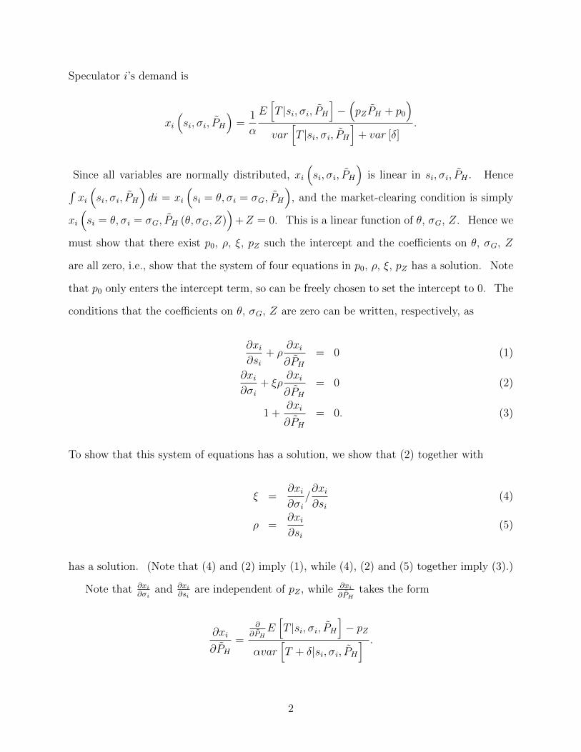
Speculator i’s demand is

xi

(si, σi, P̃H

)=

1

α

E[T |si, σi, P̃H

]−(pZP̃H + p0

)var

[T |si, σi, P̃H

]+ var [δ]

.

Since all variables are normally distributed, xi

(si, σi, P̃H

)is linear in si, σi, P̃H . Hence

´xi

(si, σi, P̃H

)di = xi

(si = θ, σi = σG, P̃H

), and the market-clearing condition is simply

xi

(si = θ, σi = σG, P̃H (θ, σG, Z)

)+Z = 0. This is a linear function of θ, σG, Z. Hence we

must show that there exist p0, ρ, ξ, pZ such the intercept and the coefficients on θ, σG, Z

are all zero, i.e., show that the system of four equations in p0, ρ, ξ, pZ has a solution. Note

that p0 only enters the intercept term, so can be freely chosen to set the intercept to 0. The

conditions that the coefficients on θ, σG, Z are zero can be written, respectively, as

∂xi∂si

+ ρ∂xi

∂P̃H= 0 (1)

∂xi∂σi

+ ξρ∂xi

∂P̃H= 0 (2)

1 +∂xi

∂P̃H= 0. (3)

To show that this system of equations has a solution, we show that (2) together with

ξ =∂xi∂σi

/∂xi∂si

(4)

ρ =∂xi∂si

(5)

has a solution. (Note that (4) and (2) imply (1), while (4), (2) and (5) together imply (3).)

Note that ∂xi∂σi

and ∂xi∂si

are independent of pZ , while ∂xi∂P̃H

takes the form

∂xi

∂P̃H=

∂∂P̃H

E[T |si, σi, P̃H

]− pZ

αvar[T + δ|si, σi, P̃H

] .

2

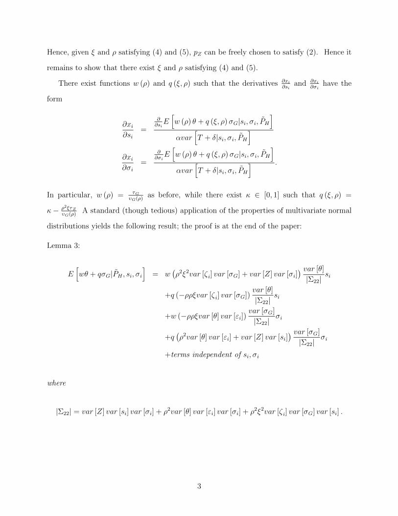
Hence, given ξ and ρ satisfying (4) and (5), pZ can be freely chosen to satisfy (2). Hence it

remains to show that there exist ξ and ρ satisfying (4) and (5).

There exist functions w (ρ) and q (ξ, ρ) such that the derivatives ∂xi∂si

and ∂xi∂σi

have the

form

∂xi∂si

=

∂∂siE[w (ρ) θ + q (ξ, ρ)σG|si, σi, P̃H

]αvar

[T + δ|si, σi, P̃H

]∂xi∂σi

=

∂∂σiE[w (ρ) θ + q (ξ, ρ)σG|si, σi, P̃H

]αvar

[T + δ|si, σi, P̃H

] .

In particular, w (ρ) = τGυG(ρ)

as before, while there exist κ ∈ [0, 1] such that q (ξ, ρ) =

κ− ρ2ξτZυG(ρ)

A standard (though tedious) application of the properties of multivariate normal

distributions yields the following result; the proof is at the end of the paper:

Lemma 3:

E[wθ + qσG|P̃H , si, σi

]= w

(ρ2ξ2var [ζ i] var [σG] + var [Z] var [σi]

) var [θ]

|Σ22|si

+q (−ρρξvar [ζ i] var [σG])var [θ]

|Σ22|si

+w (−ρρξvar [θ] var [εi])var [σG]

|Σ22|σi

+q(ρ2var [θ] var [εi] + var [Z] var [si]

) var [σG]

|Σ22|σi

+terms independent of si, σi

where

|Σ22| = var [Z] var [si] var [σi] + ρ2var [θ] var [εi] var [σi] + ρ2ξ2var [ζ i] var [σG] var [si] .

3

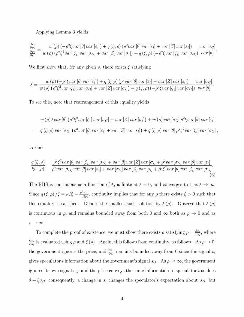
Applying Lemma 3 yields

∂xi∂σi∂xi∂si

=w (ρ) (−ρ2ξvar [θ] var [εi]) + q (ξ, ρ) (ρ2var [θ] var [εi] + var [Z] var [si])

w (ρ)(ρ2ξ2var [ζ i] var [σG] + var [Z] var [σi]

)+ q (ξ, ρ) (−ρ2ξvar [ζ i] var [σG])

var [σG]

var [θ].

We first show that, for any given ρ, there exists ξ satisfying

ξ =w (ρ) (−ρ2ξvar [θ] var [εi]) + q (ξ, ρ) (ρ2var [θ] var [εi] + var [Z] var [si])

w (ρ)(ρ2ξ2var [ζ i] var [σG] + var [Z] var [σi]

)+ q (ξ, ρ) (−ρ2ξvar [ζ i] var [σG])

var [σG]

var [θ].

To see this, note that rearrangement of this equality yields

w (ρ) ξvar [θ](ρ2ξ2var [ζ i] var [σG] + var [Z] var [σi]

)+ w (ρ) var [σG] ρ2ξvar [θ] var [εi]

= q (ξ, ρ) var [σG](ρ2var [θ] var [εi] + var [Z] var [si]

)+ q (ξ, ρ) var [θ] ρ2ξ2var [ζ i] var [σG] ,

so that

q (ξ, ρ)

ξw (ρ)=

ρ2ξ2var [θ] var [ζ i] var [σG] + var [θ] var [Z] var [σi] + ρ2var [σG] var [θ] var [εi]

ρ2var [σG] var [θ] var [εi] + var [σG] var [Z] var [si] + ρ2ξ2var [θ] var [ζ i] var [σG].

(6)

The RHS is continuous as a function of ξ, is finite at ξ = 0, and converges to 1 as ξ → ∞.

Since q (ξ, ρ) /ξ = κ/ξ − ρ2τZυG(ρ)

, continuity implies that for any ρ there exists ξ > 0 such that

this equality is satisfied. Denote the smallest such solution by ξ (ρ). Observe that ξ (ρ)

is continuous in ρ, and remains bounded away from both 0 and ∞ both as ρ → 0 and as

ρ→∞.

To complete the proof of existence, we must show there exists ρ satisfying ρ = ∂xi∂si

, where

∂xi∂si

is evaluated using ρ and ξ (ρ). Again, this follows from continuity, as follows. As ρ→ 0,

the government ignores the price, and ∂xi∂si

remains bounded away from 0 since the signal si

gives speculator i information about the government’s signal sG. As ρ→∞, the government

ignores its own signal sG, and the price conveys the same information to speculator i as does

θ + ξσG; consequently, a change in si changes the speculator’s expectation about σG, but

4

the effect is finite (and moreover, var[T |si, σi, P̃H

]remains bounded away from 0).

Increased informativeness under transparency

Writing ρ = ∂xi∂si

explicitly, price informativeness when the government does not disclose σG

is given by the solution to

αρ =

(w (ρ)

(ρ2ξ (ρ)2 var [ζ i] var [σG] + var [Z] var [σi]

)+ q (ξ (ρ) , ρ) (−ρ2ξ (ρ) var [ζ i] var [σG])

) var[θ]|Σ22|

var[T |si, σi, P̃H

]+ var [δ]

.

(7)

If instead the government makes its signal σG public, i.e., transparency, price informativeness

is determined by the solution to

αρ =w (ρ) ∂

∂siE [θ|si, P ]

var [T |si, P ] + var [δ]. (8)

To establish the result, we show that, for any ρ, the RHS of (7) is strictly less than the RHS

of (8). It is immediate that, for any ρ, the denominator in (8) is less than the denominator

in (7). The main step in the proof is to show that the the numerator in (7) is less than the

numerator in (8).

Expanding, the numerator in (8) is

w (ρ) τ ετ θ + τ ε + ρ2τZ

=w (ρ) var [θ] var [Z]

var [εi] var [Z] + var [θ] var [Z] + ρ2var [θ] var [εi].

Define

D (ρ) = var [εi] var [Z] + var [θ] var [Z] + ρ2var [θ] var [εi]

= var [si] var [Z] + ρ2var [θ] var [εi] .

5

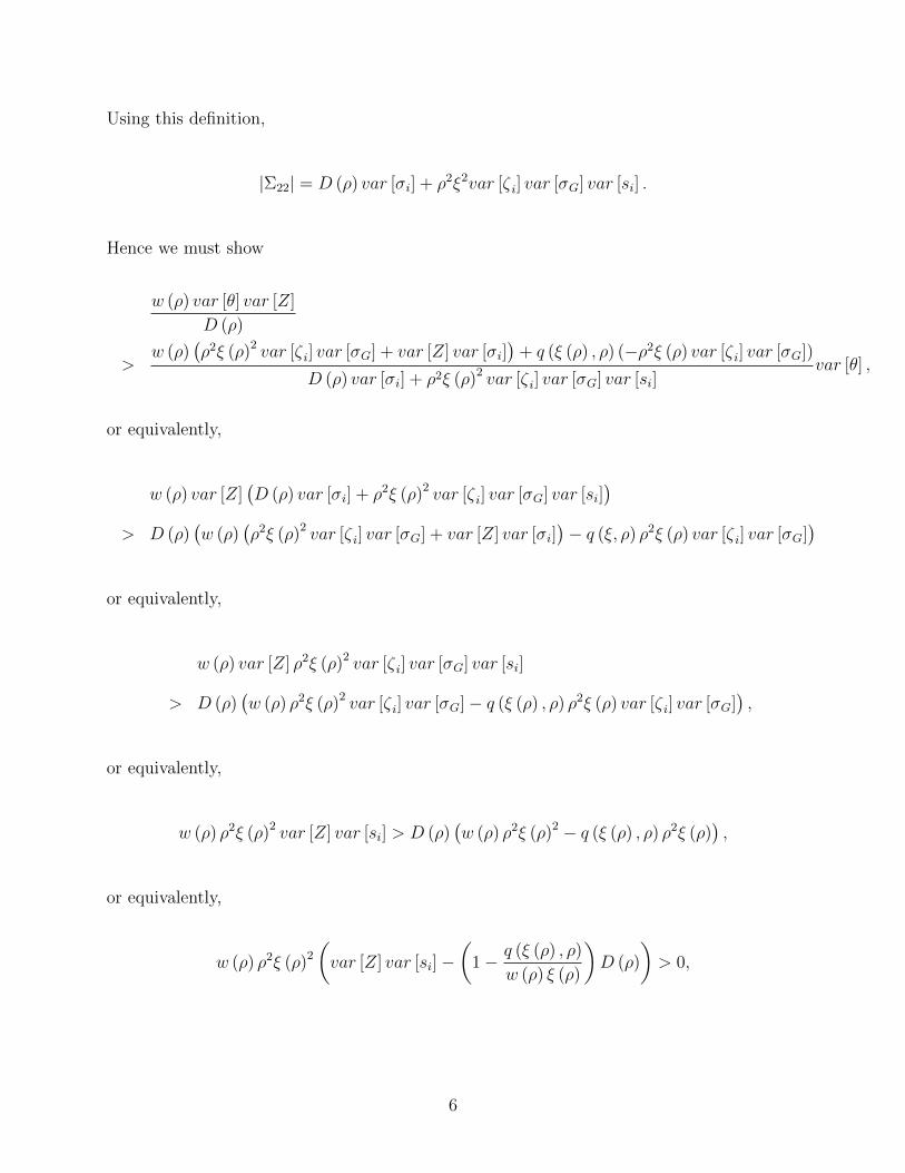
Using this definition,

|Σ22| = D (ρ) var [σi] + ρ2ξ2var [ζ i] var [σG] var [si] .

Hence we must show

w (ρ) var [θ] var [Z]

D (ρ)

>w (ρ)

(ρ2ξ (ρ)2 var [ζ i] var [σG] + var [Z] var [σi]

)+ q (ξ (ρ) , ρ) (−ρ2ξ (ρ) var [ζ i] var [σG])

D (ρ) var [σi] + ρ2ξ (ρ)2 var [ζ i] var [σG] var [si]var [θ] ,

or equivalently,

w (ρ) var [Z](D (ρ) var [σi] + ρ2ξ (ρ)2 var [ζ i] var [σG] var [si]

)> D (ρ)

(w (ρ)

(ρ2ξ (ρ)2 var [ζ i] var [σG] + var [Z] var [σi]

)− q (ξ, ρ) ρ2ξ (ρ) var [ζ i] var [σG]

)or equivalently,

w (ρ) var [Z] ρ2ξ (ρ)2 var [ζ i] var [σG] var [si]

> D (ρ)(w (ρ) ρ2ξ (ρ)2 var [ζ i] var [σG]− q (ξ (ρ) , ρ) ρ2ξ (ρ) var [ζ i] var [σG]

),

or equivalently,

w (ρ) ρ2ξ (ρ)2 var [Z] var [si] > D (ρ)(w (ρ) ρ2ξ (ρ)2 − q (ξ (ρ) , ρ) ρ2ξ (ρ)

),

or equivalently,

w (ρ) ρ2ξ (ρ)2

(var [Z] var [si]−

(1− q (ξ (ρ) , ρ)

w (ρ) ξ (ρ)

)D (ρ)

)> 0,

6

or equivalently (using w (ρ) > 0),

q (ξ (ρ) , ρ)

w (ρ) ξ (ρ)> 1− var [Z] var [si]

D (ρ)=ρ2var [θ] var [εi]

D (ρ).

Substituting in (6), along with the definition of D (ρ), this inequality is in turn equivalent to

ρ2ξ (ρ)2 var [θ] var [ζ i] var [σG] + var [θ] var [Z] var [σi] + ρ2var [σG] var [θ] var [εi]

var [σG]D (ρ) + ρ2ξ (ρ)2 var [θ] var [ζ i] var [σG]

>ρ2var [θ] var [εi]

D (ρ),

or equivalently,

ρ2ξ (ρ)2 var [θ] var [ζ i] var [σG] + var [θ] var [Z] var [σi]

ρ2ξ (ρ)2 var [θ] var [ζ i] var [σG]>ρ2var [θ] var [εi]

D (ρ).

This is indeed the case since the LHS is above 1 and the RHS is below 1, completing the

proof.

Standard analysis of multivariate normal

Proof of Lemma 3: Define

Σ22 =

var

[P̃H

]cov[P̃H , si

]cov[P̃H , σi

]cov[si, P̃H

]var [si] cov [si, σi]

cov[σi, P̃H

]cov [σi, si] var [σi]

=

var

[P̃H

]ρvar [θ] ρξvar [σG]

ρvar [θ] var [si] 0

ρξvar [σG] 0 var [σi]

.

and

Σ12 =

cov[θ, P̃H

]cov [θ, si] cov [θ, σi]

cov[σG, P̃H

]cov [σG, si] var [σG]

=

ρvar [θ] var [θ] 0

ρξvar [σG] 0 var [σG]

.

7

Then

E[wθ + qσG|P̃H , si, σi

]=

(w q

)Σ12Σ−1

22

P̃H

si

σi

.

Evaluating

Σ−122 =

1

|Σ22|

var [si] var [σi] −ρvar [θ] var [σi] −ρξvar [σG] var [si]

−ρvar [θ] var [σi] var[P̃H

]var [σi]− (ρξvar [σG])2 ρvar [θ] ρξvar [σG]

−ρξvar [σG] var [si] ρvar [θ] ρξvar [σG] var[P̃H

]var [si]− (ρvar [θ])2

,

where

|Σ22| = var[P̃H

]var [si] var [σi]− (ρvar [θ])2 var [σi]− (ρξvar [σG])2 var [si]

= var [Z] var [si] var [σi] + ρ2var [θ] var [εi] var [σi] + ρ2ξ2var [ζ i] var [σG] var [si] .

So

Σ12Σ−122

0

1

0

=1

|Σ22|Σ12

−ρvar [θ] var [σi]

var[P̃H

]var [σi]− (ρξvar [σG])2

ρvar [θ] ρξvar [σG]

=

var [θ]

|Σ22|

−ρ2var [θ] var [σi] + var[P̃H

]var [σi]− (ρξvar [σG])2

−ρρξvar [σi] var [σG] + ρρξvar [σG]2

=

var [θ]

|Σ22|

ρ2ξ2var [ζ i] var [σG] + var [Z] var [σi]

−ρρξvar [ζ i] var [σG]

8

where the final inequality follows from

−ρ2var [θ] var [σi] + var[P̃H

]var [σi]− (ρξvar [σG])2

= −ρ2var [θ] var [σi] +(ρ2var [θ] + ρ2ξ2var [σG] + var [Z]

)var [σi]− (ρξvar [σG])2

=(ρ2ξ2var [σG] + var [Z]

)var [σi]− (ρξvar [σG])2

= ρ2ξ2var [ζ i] var [σG] + var [Z] var [σi] .

Similarly,

Σ12Σ−122

0

0

1

=1

|Σ22|Σ12

−ρξvar [σG] var [si]

ρvar [θ] ρξvar [σG]

var[P̃H

]var [si]− (ρvar [θ])2

=

var [σG]

|Σ22|

−ρvar [θ] ρξvar [si] + var [θ] ρvar [θ] ρξ

−ρξvar [σG] ρξvar [si] + var[P̃H

]var [si]− (ρvar [θ])2

=

var [σG]

|Σ22|

−ρρξvar [θ] var [εi]

ρ2var [θ] var [εi] + var [Z] var [si]

where the final inequality follows from

−ρξvar [σG] ξρvar [si] + var[P̃H

]var [si]− (ρvar [θ])2

= −ρ2ξ2var [σG] var [si] +(ρ2ξ2var [σG] + ρ2var [θ] + var [Z]

)var [si]− ρ2var [θ]2

=(ρ2var [θ] + var [Z]

)var [si]− ρ2var [θ]2

= ρ2var [θ] var [εi] + var [Z] var [si] .

The result follows. QED

9