GPGPU in Medical Imaging Applications

Kevin Gorczowski

Overview

Random Walks for Interactive Organ Segmentation in Two and Three Dimensions

Interactive, GPU-Based Level Sets for 3D Brain Tumor Segmentation

Image Registration by a Regularized Gradient Flow

Accelerating Popular Tomographic Reconstruction Algorithms on Commodity PC Graphics Hardware

GPUs and Medical Imaging

Computations involving 2D and 3D images Already a natural fit for use of GPUs

Often involve numerical computations ODEs and PDEs Numerical accuracy not always top priority Visually correct and speed most important

Image Segmentation

Find the boundary or interior of a specific organ or structure

Hand-tracing still a standard clinical practice Example use: radiation cancer treatment

Take CT scan on initial day Segment organ Use segmentation to aim radiation Problem: organs move between days! Hand-tracing much too time consuming to do each

day

Random Walks for Interactive Organ Segmentation in Two and Three Dimensions (2005)Goal: Segmentation using only

small amount of user interactionUser specifies seed points

Seeds labeled according to organ/structure

Segmentation propagates toward seed points

Seed and Segmentation Examples

Seeds: gray Segmentations: black

Methodology

Unlabeled pixels (non-seeds) Send out random walker Determine probability that random

walker will reach a labeled pixel first, ahead of all other labels

Assign pixel maximum probability label

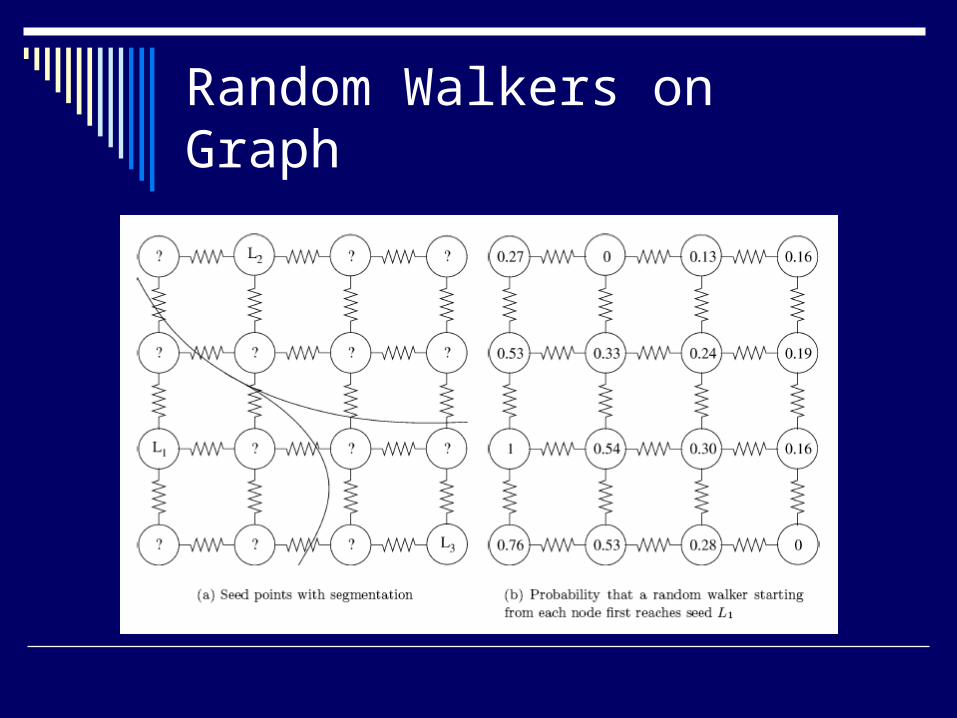
Random Walkers on Graph

Formulating Images as Weighted Graphs Nodes: pixels Edges: between neighboring pixels Edge weight: function of intensity

difference between pixel and its neighbor Weight function

g: pixel intensity, β: free parameter Able to use same β throughout

Solution

Probability of random walker reaching seed point same as solution to Dirichlet problem Partial differential equation on interior of region with

conditions at boundary of region Boundary conditions at seed pixels

1 if seed pixel belongs to label being searched for 0 otherwise

Computation of solution involves solving linear system with graph Laplacian matrix

GPU Implementation

Linear system LX = -BM must be solved for each seed label

Only M, seed boundary conditions, changes

Can use RGBA channels to solve for 4 labels simultaneously

Progress of segmentation can be updated on screen

GPU Implementation

L is symmetric and diagonal is determined by off-diagonal elements Can store L as size n = # of pixels, instead

of n x n Textures are same size as original images

Linear system solved using conjugate gradient Only matrix-vector product and vector

inner-product required

Interactive, GPU-Based Level Sets for 3D Brain Tumor Segmentation (2003) Uses deformable model approach Before, started with pixel seeds and

labeled pixels individually Here, start with template model of

organ/structure Deform model to fit target image Resulting model represents boundary

Deformable Models

Two classes of deformable shape models Parametric

Parameterized curves or surfaces Spherical harmonics, wavelets

Geometric Curves as embedded, implicit level sets of

higher-dimensional functions Can change topology (may or may not be

advantage depending on application)

Level Sets

Curve or surface: all points such that some function φ(x) = 0

φ: R3 -> R, x: position Can describe motion (deformation) as

PDE

v(t): pixel-wise velocities Implement deformations by choosing v’s

Velocities for Segmentation

Velocities usually have two components when used for segmentation Data term Smoothness term

Data term drives curve toward boundaries Typically areas of high contrast in image

Smoothness term constrains curve from becoming too irregular Prevents “leaking” out of small discontinuities in

image edges

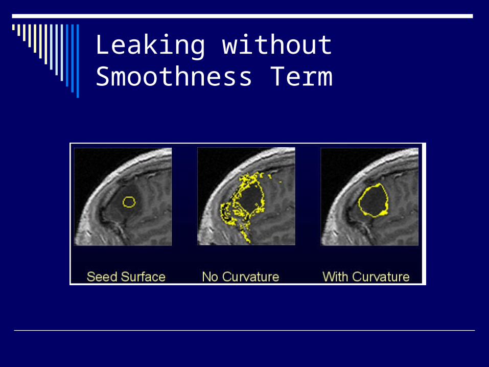
Leaking without Smoothness Term

Problems

Data term usually introduces free parameters Their data term: I: image intensity ε: determines range of values considered inside

object T: determines how bright object is Basically, T is mean intensity and ε is variance User has to choose these free parameters If segmentation runs at interactive speed

(GPU), user can be much more productive

GPU Implementation Issues

For stability, curve must move at most one pixel at each iteration Results in many iterations before solution Need to keep as much on GPU as possible

Major speedup if only places where φ is close to zero are considered How to pack for GPU Changes after each iteration

Data Packing

Subdivide data into 16x16 tiles Only tiles with non-zero derivatives sent

to GPU

Data Packing

Evaluation of PDE requires discrete derivatives Pixels need to access neighbors

CPU calculates and sends texture coordinates of neighbor pixels in packed format

GPU does neighbor lookups and finite differences used for gradient and curvature

CPU also sends vertices of active tiles for quad rendering

Data Packing

CPU needs to active tiles for each iteration so it can calculate neighbor pixels

GPU writes out a small (<64KB), encoded texture telling which tiles are active Checks if a tile boundary has been crossed

Limits CPU <-> GPU bus use

Performance

CPU: 1.7GHz Xeon 7-8 iterations/sec “Highly-optimized, sparse-field, CPU-based solver"

Radeon 9700 Pro 60-70 iteration/sec

Running time of GPU implementation scales linearly with number of active voxels

Overhead for feedback image calculation about 15% of total GPU time

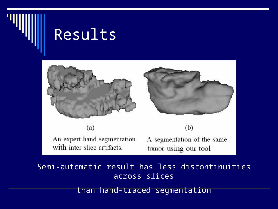
Results

Semi-automatic result has less discontinuities across slices

than hand-traced segmentation

Movies

Image Registration by a Regularized Gradient Flow (2004)

Image registration Try to get intensities in multiple

images to match spatially Simple case: use similarity

transforms to align images as best as possible

Complex case: non-rigid registrationEach pixel has its own displacement

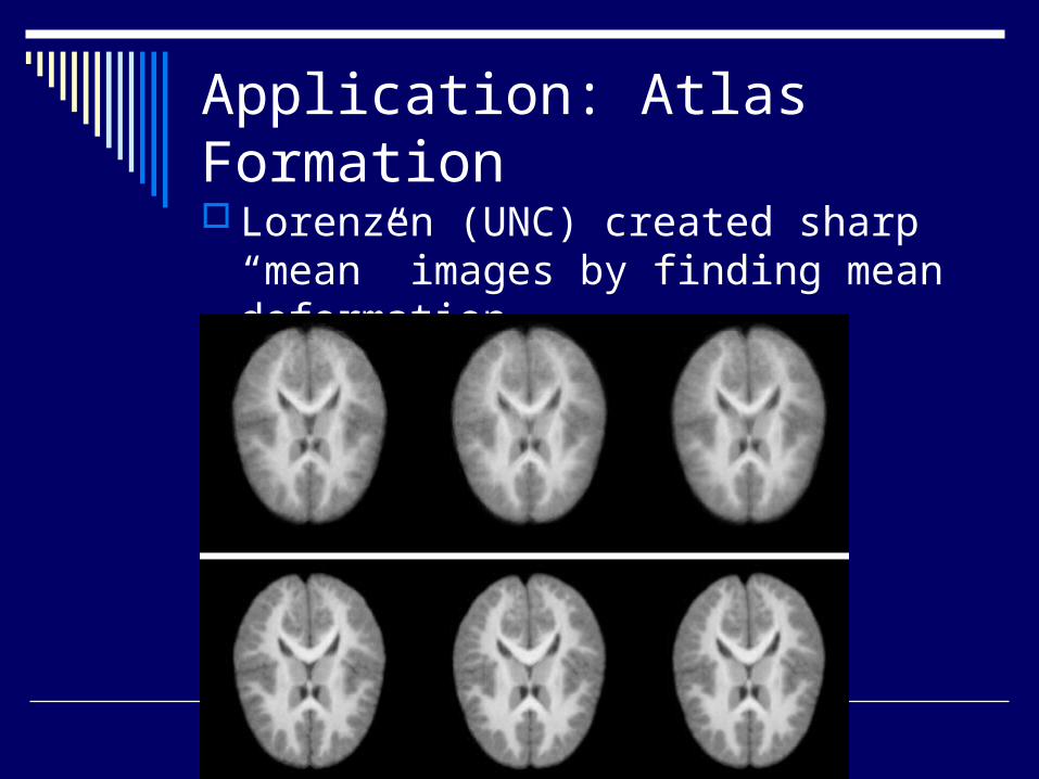
Application: Atlas Formation

Lorenzen (UNC) created sharp “mean” images by finding mean deformation

Registration Formulation

Must define a measure of how closely two images match

Can formulate as an energy function

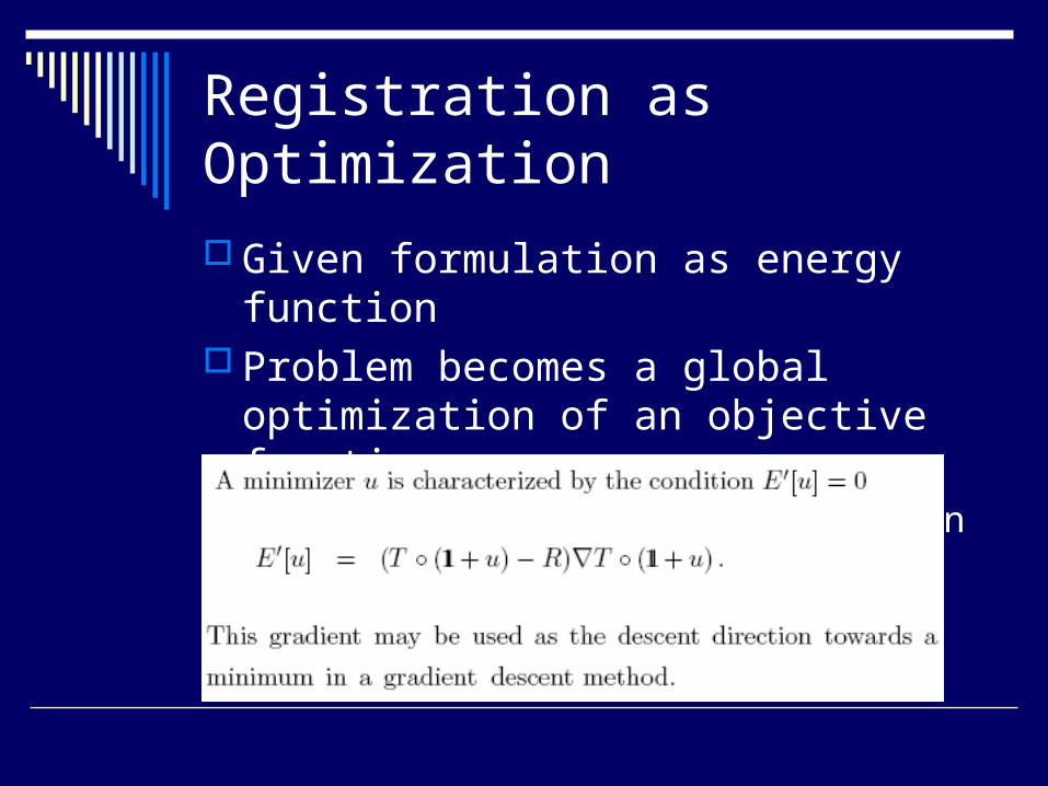
Registration as Optimization

Given formulation as energy function Problem becomes a global optimization

of an objective function Find minimum of energy function

Uniqueness of Solution

Discretization

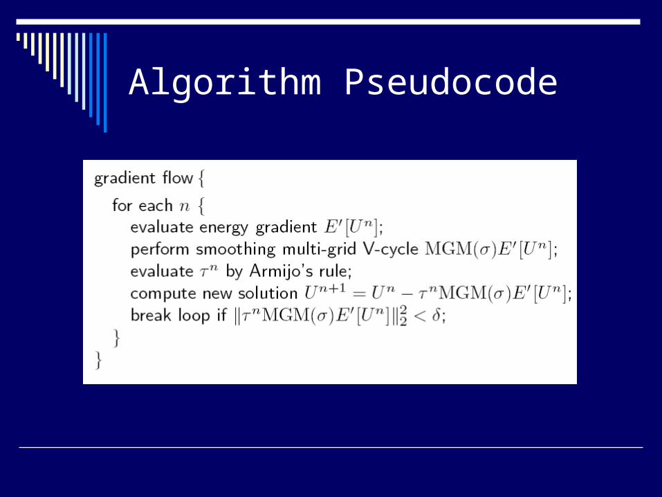
Algorithm Pseudocode

GPU Implementation

Results

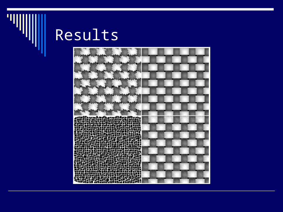
Results

Results

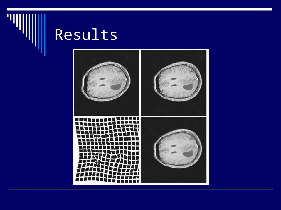
Results

Performance

Accelerating Popular Tomographic Reconstruction Algorithms on Commodity Graphics Hardware

Computed Tomography CT scan, used to be CAT scan

X-ray source Object attenuates x-rays Collector (2D sheet) measures

left-over radiation Source and collector rotate

around object

Reconstruction

Only information acquired through scan is 2D “image” at collector

Have collector image for each angle φ (position of source/collector on circle)

Must solve for attenuation of scanned object at points on 3D grid

Formulation

Amount of radiation collected at pixel (u,v) of collector for angle φ

μ: attenuation (unknown) Q0: original x-ray energy at source

L: distance between source and collector Integrate attenuation along x-ray

Formulation

Rewrite i: pixel index of

collector

Voxel form (loop

through object voxel

Grid)

Formulation

wij : weight of voxel j’s contribution to detector pixel i Determined ahead of time by interpolation

and integration rules

Solving for Attenuation

Mφ : number of pixels in collector for angle φ

Know qi and wij, solve for attenuation (backprojection)

Final Image Reconstruction

Feldkamp algorithm

SART iterative

algorithm

OS-EM algorithm

GPU Implementation

Each iteration requires at least one backprojection and projection

Each backprojection is O(n3) No real way around complexity Must use brute force speed

Many CT machines use FPGAs or ASICs Expensive Inflexible

GPU Implementation

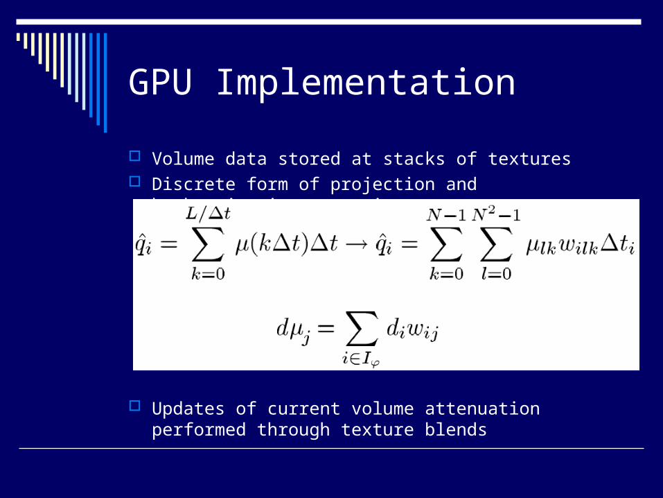
Volume data stored at stacks of textures Discrete form of projection and backprojection operations

Updates of current volume attenuation performed through texture blends

GPU Implementation

Can use RGBA channels to compute orthogonal projections Projection matrices are equal Four 90° increments of φ

Can’t do this in SART because of incremental volume updates Instead, fold volume in half (RG) Projection matrices are same except for

reflection

Results

Performance

References

Leo Grady, Thomas Schiwietz, Shmuel Aharon, Rudiger Westermann, "Random Walks for Interactive Organ Segmentation in Two and Three Dimensions: Implementation and Validation", Proceedings of MICCAI 2005, vol. 2, 2005, pp. 773-780.

Aaron E. Lefohn, Joshua E. Cates and Ross T. Whitaker, “Interactive, GPU-Based Level Sets for 3D Segmentation”, Proceedings of MICCAI 2003, vol. 2, 2003, pp. 564-572.

Robert Strzodka, Marc Droske, and Martin Rumpf. “Image Registration by a Regularized Gradient Flow - A Streaming Implementation in DX9 Graphics Hardware.” Computing, 73(4):373–389, 2004.

Fang Xu, Mueller, K. “Accelerating Popular Tomographic Reconstruction Algorithms on Commodity PC Graphics Hardware.” IEEE Transactions on Nuclear Medicine. Volume 52, Issue 3, Part 1, June 2005. pp. 654- 663.