GPS Kinematic Positioning for the Airborne Laser Altimetry

at Long Valley, California

by

Gang Chen

B.S., Astronomy (1986)Nanjing University

M.S., Astronomy (1989)Shanghai Observatory, Ch1nese Academy of S~ience

Submitted to the Department of Earth, Atmospheric, and planetarySciences in partial fulfillment of the requirements for the degree of

Doctor of Philosophy in Geophysics

at the

MASSACHUSETTS INSTITUTE OF TECHNOLOGY

Nov. 1998.. I ,-, '

© 1998 Massachusetts Ihstitute of~Technology.

All RIghts Reserved.

Author ••••••••••••••••••• 0 •••••••••• , ~.-.:'••~.~. rI••••• ...-:-••• ~ .""':"'.':"".; • .;''";';-:''''; •••••••••••••••••••••••••••••••

Department of Earth, Atmospheric, and Planetary SciencesJune 19,1998

MASSACHUSETTS INSTITUTE_ OF TECHNOLOGY

Certified by 1' •••••••••••••••••••••••••••••••••

Thomas A. HeningThesis Supervisor

Accepted by ~ .Ronald G. Prinn

Department Head

r~AR 3 1 1999

LIBRARIES

GPS Kinematic Positioning for the Airborne Laser Altimetryat Long Valley, California

by

Gang Chen

Submitted to the Department of Earth, Atmospheric, and Planetary Scienceson June 19, 1998 in partial fulfillment of the requirements for the degree of

Doctor of Philosophy in Geophysics

Abstract

The object of this thesis is to develop a reliable algorithm and soft\vare for em-levelkinematic GPS (Global Positioning System) data analysis. To assess the accuracy of thesoftvlare, we use it to determine the trajectory of the aircraft during the surveys at Long Valley,California, in 1993 and 1995. This thesis covers the algorithm development, the modeling, andthe software design. We implement a robust Kalman filter to perfonn the kinematic dataprocessing for GPS measurements. In the kinematic data processing with the Kalman filter, theestimates of the aircraft's position, the GPS receiver clock, and atmospheric corrections aremodeled with appropriate stochastic processes.

To achieve em-level accuracy for an aircraft trajectory, the GPS phase observables mustbe used and the integer-cycles of phase ambiguity must be resolved. In this thesis, we investigatethe ambiguity problem in different situations and develop different ambiguity strategiesdepending on the situation. Firstly, we develop a position-independent (position-free) ambiguitysearch method for the initial ambiguity search for GPS kinematic surveying. Our ambiguitysearch method focuses on providing the flexibility and uniqueness to determine the correctambiguities in most experimental conditions including long baselines (up to 100 km), high noiselevel in low elevation observations, and "bad" observations during the search. Secondly, wedevelop a method to utilize position-free widelane and extrawidelane observables to detect cycleslips that occur when the signal from a GPS satellite is interrupted during the flight, for example,when the satellite is blocked by the aircraft's wing during a turn. Our ambiguity algorithms usedual frequency GPS observables so that the effects of the ionospheric delay can be accounted for.Several tests perfonned indicate that our ambiguity strategy works well for a separation betweenthe moving and fixed GPS receivers of up to 100 lan.

We developed a killematic sofuvare developed to automatically detect various errorsduring the data processing, including detecting and correcting of cycle slips, detecting andremoval of bad data, and performing ambiguity searches. 1be user interface to the software iscommand driven with default values for most processing. This interface provides flexibility andshould make the software usable with little training.

To evaluate our software, we processed GPS data taken in the 1993 and 1995 LongValley airborne laser altimetry surveys. We performed four types of tests: (a) Static tests which

3

the evaluate the root-mean-square (RMS) scatter of the aircraft position \vhile it is stationary onthe run-vvay; (b) runway tests vvhich compare the height estimates of the aircraft at approximatelythe same position along the ruIlway during taxiing, ta!ceoffs and landings; (c) lake tests in whichwe compare profiles of Lake Crowley"s surface and crossings on the lake surface; and (d) Bentoncrossing tests in which we compare surface height estimates at location within 2 m of each otherat a grassy region of Benton Crossing. The latter two tests use of combination of the laseraltimeter and GPS trajectory data. The processing of the laser data with our GPS trajectory wasperfonned by our colleagues at the Scripps Institute of Oceanography.

The static tests show that during the times the aircraft was stationary at the beginning andends of flights, the R..MS scatter of relative height difference between the aircraft and thereference GPS station at Bishop airport, approximately 500 meters from the aircraft, variedbetween 4 and 2 mm for both campaigns. The lUi"1Way tests show that the average heightditIerences between trajectories repeat to within 4 em for six tracks on the taxiway, during thetakeoffs and landin[...... The lake surface tests show height variations within 3 em for fne lakesurface after removing the cubic polynomial to approximately fit for the geoid-ellipsoidal heightdifferences and flow within the lake for each of the five flight sections over the lake. ~fhe LakeCrowley crossover analysis shows a mean difference of 0.2 em and RMS scatter of 4.5 cm forrelative height from laser footprint pairs within 2 m distBllce. The Benton Crossing crossoverresults show a mean value of 0.2 em and R...MS scatters of 15.5 cm in a similar cross analysisafter outliers are deleted. Based on our analyses, we conclude t.~at laser altimetry over the flatsurface (i.e. Lake Crowley) can detennine surface heights with --3 cm precision. Thecontribution from the error in GPS trajectory appears to be 1-2 em.

Thesis supervisor:

Title:

COIrilllittee:

Thomas A. Herring

Professor of Geophysics

Professor Thomas A. HerringDr. Robert W. KingProfessor Chris J. MaroneProfessor Jean-Bernard I\1inster

4

Acknowledgments

The completion of this thesis would not have been possible without the support of many

people.

First, I WQ1lld like to thank my advisor, Tom Herring, not only for his guiding the prepara­

tion in this thesis, but also for his continuing support, and encouragenlent through five years at

MIT_He was always willing to share his insights with me and was patient with every questions.

From TOlTI, I learned a lot, fron.1 hovv GPS works for geodesy to how to make the plots more col­

orful. Also I am grateful for the freedom he gave me to explore and develop my own ideas.

lowe a special thank to Adrian Borsa. Without his help in the ATLAS data analysis, I

could not have finished Chapter 5 of this thesis. He has spent a great deal of his time going

through the data analysis with my nllffierous tests. J would also like to thank Michelle Hofton for

her time spent with me discussing the GPS processing at NASA Goddard Space Flight Center

(GSFC) and providing data, information and suggestions wheIlever I wanted. I am indebted to

Prof. Bernard Minster and his group for allowing Ine use the data and for inviting me to the field

test in Long Valley. I have enjoyed working with them.

I would like to thank Bob King for his critical comments a.lld discussions on the thesis

which not only made my ill-written sentences more readable, but also led me to a better lUlder­

standing of the GPS system.

My L.~anks also go to Arthur Niell for providing mapping fimction code, to Paul Tregoning

for his comments and tests on the use of the first versiOll of my GPS kinematic software~ to Ming

Fang, Brad Hager, Clint Conrad, Katy Quinn, Simon McClusky and other 6th floor colleagues for

sharing their geophysical knowledge, computer tricks and fun; To elmS Marone, I am grateful for

the chance to take his interesting course and to do friction research with his instruction; To Ben

Chao for the invitation to visit NASA GSFC, and for discussions covering a broad scope of prob­

lelns in the Earth sciences.

1 would like to express my gratitude to my parents. For the post five years, their endless

5

support and understanding fron1 the remote other side of Earth has meant a lot to their son. Also

thanks to my sister for her encouraging me cross the Pacific and helping me take care of our par-

ents.

Finally, the person I wish to thank most is, my wife, Wei Zhu, who made my jounley to

I\1IT not lonely, and fills my heart with confidence, courage, and love all the time.

This work \\t·as supported by NASA grants NAGS-3550 and NASS-33017.

6

Table of Contents

1 Inti4 oduction 111.1 Kinematic GPS Surveying ~ ~ 111.2 Geodetic measurements at Long Valley 131.3 Laser Altimetry - 161.4 Role of GPS in Airborne Altimetry 17

2 Kalman Filter Algorithm in GPS Analysis 252.1 Itltroduction 252.2 Discrete Kalman Filter Algorithm · u 282.3 GPS Observations 33

2.3.1 Pseudorange Observations 332.3.2Carrier Phase Observations 342.3.3 Single and Double Differencing 352.3.4 Linear Combipations of Observations 37

2.4 Model 392.4.1 Position and Velocity Model 422 ..4.2 Clock Model 432.4.3 Atmospheric Model 44

3 Phase Ambiguity Resolution Strategy u513.1 Introduction 513.2 Initial Ambiguity Search Strategy 56

3.2.1 Utilization of Dual Frequency Information 563.2.2 Strategy of Initial Ambiguity Search 57

3.3 Tests for Initial .wbiguity Search 663.3.1 Applicrtion in Short Baselines 663.3.2 Application for a Middle Range Baseline 70

3.4 AInbiguity Resolution for New Satellites u ••• ~ 723.5 Cycle Slip Detection and Fixing 00 743.6 Software Design 75

4 Kinematic GPS Data Analysis 1014.1 Long Valley Surveys a ••••••••••••••••••••• 1014.2 Software Use and Data Handling 1044.3 Kinematic GPS Data Processing and Analysis l 084.4 Calibration Analysis on the Airport 111

4.4.1 Airport Static Tests 1 1114.4.2 Runway Kinematic Tests 1 ~ 112

5 Validation ofGPS Trajectory from ATLAS Measurements 1475.1 ATLAS Data Analysis 1475.2 Calibration over Lake Crowley 1485.3 Crossover Analysis 150

7

5.3.1 Lake Crowlay 1505.3.2 Benton Crossing 151

6 Discussion and Conclusion 163

Appendix A AtTI10Spheric Delay Modeling n 169

8

9

10

Chapter 1 Introduction

The object of this thesis is to develop a reliable algrJrithm and software for em-level

kinematic GPS rlata analysis and to assess its accuracy in detennj.ning tile trajectories for

airborne laser altimetric surveys at Long Valley, California. The availability of precise laser

altimeter data provides us with a unique oppommity to evaluate tI1e accuracy of the aircraft

kinematic trajectory during flight.

1.1 Kinematic GPS Surveying

Global Positioning System (GPS) has been widely used in navigation, tlmmg and

surveying for over 20 years. In geodetic and geophysical fields, GPS also provides a tool for high

precision measurements of plate motions, tectonic deformation and volcanic monitoring. Recent

results show few mrn-Ievel accuracy for position determinations in some GPS networks [Alber

et. ai, 1997].

In kinematic differential GPS surveying one GPS antenna is nonnally moving with a

vehicle or an aircraft while the other remains stationary at a ground reference station. Both

antennas record the GPS signals continuously so than the relative positions of the antennas can

be determined by differential data processing. The mobility and rapidity of kinematic GPS

surveying provides numerous opportunities for precise quantitative studies such as rapid

surveying cross faults shortly after earthquakes [Hirahara et al. ~ 1996; Genrich et aI., 1997],

position controlling for airborne photogrammetry [Ackermann, 1992; Becker and Barriere,

1993], and seismic explosi\~e source positioning on the ocean [Chapman et al., 1997; Tregoning

et al., 1998]. Besides its direct applications, precise kinematic GPS can be also used to improve

the accuracy of other techniques. Without the em-level accuracy of kinematic GPS positioning

for aircraft, for example, it is impossible for the airborne laser altimeter tectmique to monitor cm­

level variations of ground displacement.

I 1

The common observables of GPS are pseudorange (time difference between transmIssion

and reception of signal with the transmission time set by the satellite clock and reception time

measured with a non-synclrronized ground clock) and carrier beat phase (difference between the

received phase and the phase generated from local oscillator of receiver)n Doppler measurements

are also available but not used here. For em-level measurements, carrier phase is generally used

because it is much more precise than pseudorange. Carrier phase is most llseful, however, when

there are long tracks of uninterrupted tracking of a satellite so that the change in range to the

satellite may be used for positioning. Also, dual frequency measurements are needed to remove

the frequency-dependent (dispersive) ionospheric effects on GPS signals.

Several data analysis methods have been developed which depend on the use of different

observables. TJtilizing the code signals directly received from satellites, point positioning is

widely used in general surveys but needs knowledge of satellite clock errors as well as orbital

position infonnation. By comparing the signals from the same satellite at t\\'O GPS receivers,

differential positionillg (single difference) removes effects of the unknown satellite clock. The

comparison of single-difference observables from two satellites (double differencing) can

remove the re.;eiver's clock \'ariation. For close stations, marlY other errors such as orbital errors,

ionospheric delays, tropospheric delays, and earth tide effects, also cancel to a large degree in

differential method. pseudorange differential positioning is used but limited by measurement

accuracy. Carrier phase differential method with static receivers can use changes in phase to

make more accurate positioning, but the most accurate results are obtained if the ambiguities in

the double differences can be resolved.

As a surveying technique, kinematic GPS has wide applications but also stringent

requirements. Compared to stati'c GPS surveys, the occupation time is shorter and the amount of

data accumulated is less in the kinematic applications. Also the rapid changes of environment

around the moving GPS antenna tend to create more technical problems than occur in a static

survey at a fixed site. The impact of these problems can be severe in aircraft applications where

the motions are rapid and the aircraft can fly a large distance from the base station. For kinematic

positioning, resolving cycle ambiguities is critical. The fast mo\~ement of aircraft can make

tracking more difficult for receivers, leading to corrupt data than for the static case.

12

The use of kinematic GPS technique requires a reliable and fast algorithm for the GPS

data analysis. One of the primary motivations for this study is to develop GPS analysis software

to help scientists, especially for those involved in the Long Valley airborne laser altimetric

experiments, to whom GPS is merely a secondary tool, to process smoothly kinematic GPS data.

For easy but reliable use, saftware for aircraft positioning must have the following features: a)

the software must resolve the ambiguities ploperly from the beginning of the survey while the

aircraft is stationary; b) for a long-distance and lorlg-time fligbt, new satellites should be used

and their ambiguities must be resolved immediately; c) Corrupted data and loss-of-Iock on

satellite signal must be detected and then either d.eleted or its cycle slip re-estimated; d) for larg~

separations, ionospheric delay must be accounted for. Ideally all of these are done autonomously

by software. In this thesis, we discuss our development of a kinematic GPS analysis program.

We also evaluate the program using data from Long valley laser altimeter campaigns.

1.2 Geodetic Measurements at Long Valley

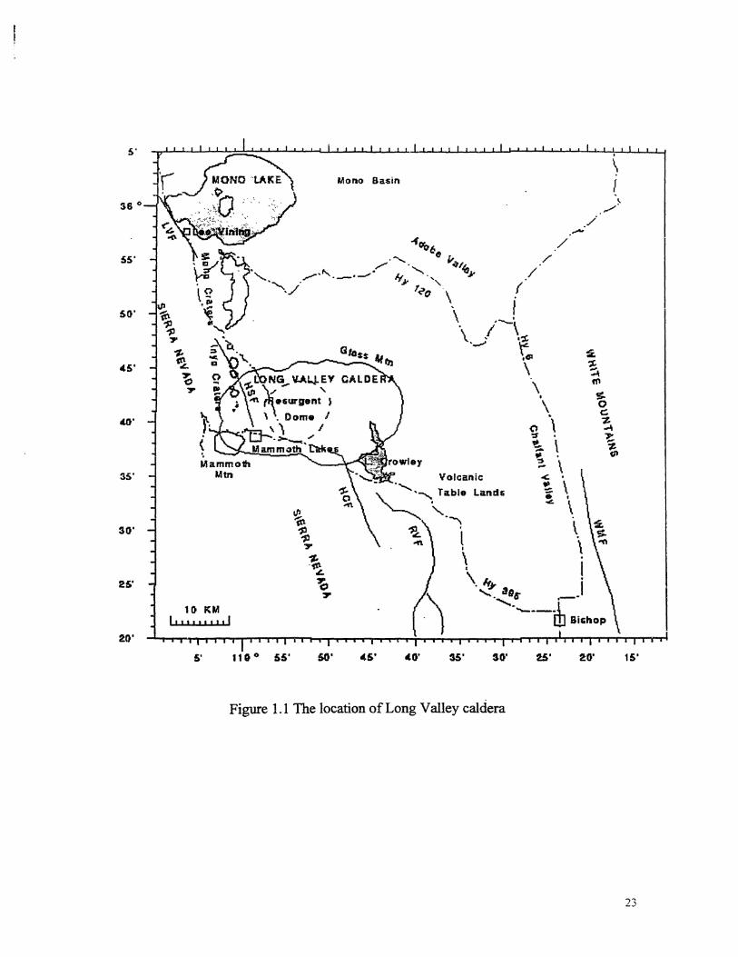
Long Valley caldera is a large volcano located 20 km south of Mono Lake along the

eastern side of the Sierra Nevada in east-central California (Figure 1.1). In this area of eastern

California, persistent earthquakes and volcanic eruptions have been occwring for over 3 million

years [Knesel and Davidson, 1997]. These activities formed the current eastern Sierra landscape

in the vicinity of Long Valley caldera. The caldera is an elliptically shaped area approximately

25 by 60 kilometers in size (the elliptical area in Figure 1.1). Ten kilometers below the stuface of

the caldera is a magma chamber [Dvorak and Dzurisin, 1997].

After Sf' years of relative quiescence:; tlle volcanic activiti~s resumed during the 1980s

aJld 1990s. The new activities started in 1980 with frequent earthquakes in the Long Valley

caldera region [Julian, 1983; Julian and Sip/dn, 1985]. The vertical surface llplift near the center

of the resurgent dome was detected at a rate of 4 to 5 em per year [Sav(,1ge et al., 1986]. Models

consistently showed that the bulk of the uplift was caused by an expanding magma reservoir 6 to

10 kn~ beneath the center of the resurgent dome, with an injection volume of about 0.15 km3

13

between 1975 and 1983 [Rundle and Whitecomb, 1984]. In 1989 a massive earthquake swarm

occurred beneath Marnmoth Mountain. Uplift increased to almost 5 em/year which can be

modeled by a re-inflation of the magma body approximately 0.025 Ian3 for the 1989-1991 period

[Langbein et aI., 1993]. These activities brought about a total uplift near 70 em in the last two

decades. This magma body l'!1ay have a total volume of 500-1,000 km3. Intensive research has

been pursued to map the distribution of magma beneath the whole area as well as its inflation

rate.

The increased activities have motivated increased monitoring in this region. Several

groups, including the U.S. Geological Survey, began monitoring the area intensively for

earthquake activity and ground deformation, in addition to conducting many detailed regional

geological and geophysical surveys in the Long Valley area. A.bout 50 pennanent seismic

stations of the Northern California Seismic Network (NCSN) are operated within 50 km of the

caldera to monitor the seismic activities. Seismometers are deployed in the Mammotll Mountain

and the southern rim of the caldera to record the seismic activities over the dome and nearby

area.

Surface height change, the uplift, in the caldera is an important indicator of volcanic

eruptions. The swface rises or falls as magma moves under the surface. The uplift plays a key

role in revealing the movement of geothennal and/or volcanic fluids under Long Valley dome.

Researchers are trying to model the rate and pattern of surface displacement. Those models

generally consist of several pressure sources embedded in an elastic material. The vertical and

horizontal displacement pattern reveals such characteristics as depth an.d rate of magma

accumulation under the ground and are needed to build up models. Besides the rapid change

before and during volcanic eruptions, long tenn changes occur near the "'lolcanic area. The

shallow magma causes the ground surface to rise or fall slowly, and those irregular changes may

be a good sensor for eruption prediction. Along with seismic activity, the slight displacements of

the surfaces are the most significant phenomena that can be monitored before and between

volcano eruptions.

14

Geodetic measurements have proven to be useful for providing information as precursors

to volcanic eruptions. Surface uplift in the caldera has been measured with Electromagnetic

Distance Measurements (EDM) since 1975 [Denlinger and Riley, 1984], and with accurate two­

color geodimeter measurements since 1983 [Langbein et aI., 1995]. Ground GPS measurements

have been also used to document changes in the reservoir and strain field over the last several

years [Dixon et al., 1993 & 1997; Marshall et 01., 1996; Webb et al., 1995]. Ground GPS

networks and leveling survey usually measure the relative positions at bench marks scattered

across the surface. Repeat measurements of the benchmarks are used to detennine the c1:J.anges in

relative positions. Such ground networks produce very precise results but do not provide good

CO\i'erage around the volcanic areas. For a typical IO-plus kilometer square volcanic area, a large

nwnber of points is needed to determine the details of surface displacement associated with the

underground magma movements. The expense of maintaining such networks could be

prohibitive for long tenn monitoring. Furthennore, the largest displacement often occurs near the

center of volcanic areas where an eruption would endanger both personal and equipnlent.

In addition to the scattered ground-based measurements, aircraft or satellite observations

could provide a valuable data source in ()btaining a dense coverage over the uplift area directly

without extensive increase of the expense and labor cost. While ground surveying can provide

precise measurenlents of changes in fi:<ed benchmarks, airborne surveying can provide less

precise but much denser measurements of profiles directly over the center of uplift areas in a

short time. In the future, an aircraft laser system can provide the capability for a rapid

topographic profiler, if needed, in response to any area with increased geologic activity,

particularly in remote or dangerous volcanic environments.

In order to test this new technology, from 1993 to 1997 researchers from several

universities and gO'vemment agencies led by the Scripps Institution of Oceanography (SIO),

NASA's Goddard Space Flight Center (GSFC) and Wallops Flight Facility (WFF), conducted

aircraft topographic surveying over the Long Valley caldera, California. Such surveys are

performed using an airborne laser system developed by WFF. The objective of this field project

was not only to measure the uplift over the resurgent dome and nearby areas of Long Valley

caldera, but also to improve and refine the equipment and analysis techrJ.qlJeS for the future

15

application of airborne and spaceborne laser altimetry.

Besides the field tests conducted by SIO, GSFC and WFF, the Long Valley survey work

also involved collaborations among many research groups at the Massachusetts Institute of Tech­

nology (MIT), Jet Propulsion Laboratory (JPL), Lawrence Livennore National Laboratory, U.S.

Geological Survey and the University of Arizona to provide technical help. The role of the MIT

team focused on the assessment of GPS data analysis for GPS aircraft tracking anc the develop­

ment of a robust and easy-to-use software package for the precise kinematic GPS surveying.

1.3 Laser Altimetry

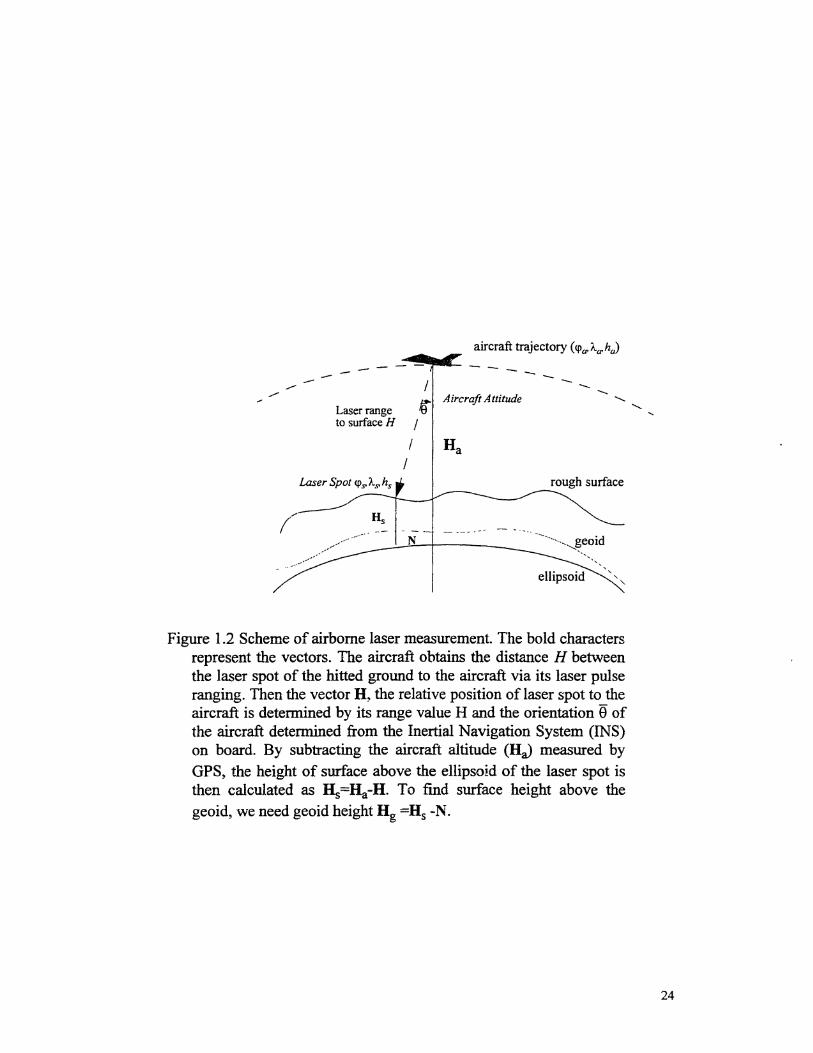
The principle of laser profiling (ranging) is shown in Figure 1.2. A short pulse (usuall)'

infrared radiation) is emitted towards the surface by the instrument in the aircraft, and its echo is

detected some time later. By measuring the time delay between the transmission and reception of

a signal and knowing the speed of propagation of the light pulse, the range (distance) from the

instrwnent to the surface can be determined. By' sending out a continuous stream of pulses, the

system can blJild up a profile of the range. If the position of the aircraft, the direction of the laser

pointing, and the relative position of the laser measurement point and GPS receiver in the aircraft

are accurately known as a function of time, the surface profile may then be deduced. The surface

heights calculated are referenced to ellipsoid (a purely geometric shape), not to the geoid

(irregular shape related to local gravity). Geoid models can be used to compute the difference

between the geoid and ellipsoid surface, i.e. the geoidal heights N in Figure 1.2. for changes in

surface height, However, the difference between the ellipsoid and geoid is not important unless

the geoid height is changing.

Laser altimeters have been successfully used on NASA space shuttle missions [Zuber et

al., 1992; Smith and Sandwell, 1994, and Smith et al., 1997]. Several laser instruments are under

development for Earth topography including the Geoscience Laser Altimetry System (GLAS)

and the Vegetation Canopy Lidar (VeL). The GLAS satellite will be placed in orbit around the

Earth in mid-2001. In recent years, in support of the spacebome missions, airborne laser

16

altimeters have been under study for their utility in profiling topographic features of the Earth.

Satellite laser altimeters have been used to profile the surface of the moon and Ma :s. Laser

altimetry utilizes a much more focused beam than equivalent radar instruments, resulting in a

smaller footprint, and is more sensitive to the angular attitude of the platfonn. The airborne laser

altimeter technology has been used to characterize the geomorphology of the volcanic island of

Surtsey, in the North Atlantic [Garvin, 1996], and has shown promise in providing height of land

surface for ~atellites in measurements of the Greenland ice sheet height [Krabill et al., 1995]

1.4 Role ofGPS in Airborne Altimetry

One of the main obstacles to the application of airborne laser altimetry is the effect of the

trajectory measurement error. The laser instrument on the aircraft measures the surface height

relative to the aircraft position directly by emitting and receiving the laser signals reflected from

the ground.. In order to obtain the surface profile variations, laser measurements have to be tied to

a well-defined solid Earth coordinate frame, for example, via differential GPS tracking of the

aircraft from ground stations. In traditional navigation systems, including the inertial navigation

system, the accuracy of position determination for aircraft is somewhere between 30 em and 2

meter, worse than the altimeter precision by a factor of ten to fifty. Without em-level precise

aircraft tracking, it is impossible for the aircraft laser technique to approach the accuracy

necessary to measure ground motions as small as 4 em per year, the expected magnitude caused

by volcanic activity at Long Valley.

The current instrument precision of GPS is capable of allowing GPS to track a moving

object with the required em-level accuracy. To reach the potential of centimeter-level kinematic

GPS surveying, however, several technical problems in the GPS data analysis have to be dealt

with carefully. To achieve the accuracy requires the integer cycle ambiguities in the carrier phase

measurements to be resolved correctly. In the mountainous areas near Long Valley, the

differencing of observations in two GPS antennas IIJ.ay not remove all of the ionospheric effects,

multipath effects (reflection from ground or objects) and other non-common model errors. These

errors can corrupt the ambiguity resolution of the phase observations. The algorithm developed

17

should provide unique ambiguity resolution in general conditions. In addition, the most complete

model of GPS observations should include pil effects larger than one centimeter for ground

distance greater than 100 km. These models include precise satellite ephemerides and height

dependent atmospheric delay models. The long experiment duration (>4 hrs) and long baselines

require that cycle sJips during flight, acquiring of new satellites ~d removal of corrupted data,

all be handled by the algorithm with minimum user interaction.

Reliable and fast software is required for the kinematic differentiJ1 GPS data analysis to

achieve its potential to the em-level in accuracy_ Many commercial software packages are

capably of the em-level accuracy for the differential GPS kinematic surveys in small areas

(baseline shorter than 10 km), but they often do not work reliably in a large area (100 km

horizontal separation and 10 km altitude difference). Analyses of the altimeter flights in Long

Valley, had used the commercial f\shtech GPS software PNAV and NASA GITAR softwar~

[Martin, 1991] to obtain the GPS trajectories [Ridgway et al., 1997; Hofton et al., 1997]. We

tested three software packages, PNAV, GITAR and our kinematic GPS software TRACK ( TRA

jectory Calulation with Kalman filter) for the September 28, 1993 survey in Long Valley.

comparing the estimated heights of the aircraft before takeoff and after landing at the airport.

TRACK and GITAR generated similar height estimates (within 1 em) after we carefully

corrected all the ambiguities of phase observations for GITAR. The after-landing height estimate

of the aircraft from the PNAV has a 5 em difference from other two programs although they are

set with the same height before the takeoff. GITAR is capable to provide em-level GPS

trajectory determination if there are no cycle slips, signal lock loss in the GPS phase

observations, and all ambiguities are reliably solved durhlg static portion of flights. Cycle slips

and changes in satellite visibility need to be handled interactively in GITAR, however, whic~

makes autonomous data processing difficult. Also GITAR has a requirement of using a common

satellite for ambiguity adjustment and double differencing and this limits its use in long-time

flights. For these reasons, we felt that it was important to develop a new algorithm that would

handle complex situations during flight and would process GPS data largely autonomously.

This thesis documents our approach to the development of algorithms, computer codes,

and analysis methods for aircraft GPS navigation for the Long Valley mission. In Chapter 2, we

18

describe our Kalman filter algorithm as well as the mathematical modeis and stochastic

properties of state variables used in the algorithm. Also we describe the software structure for

this algorithm. Chapter 3 addresses our method for the integer ambiguity resolution of carrier

phase measuremellts. We also discuss the application of this method and its validation for short

and long baselines. In Chapter 4 we rlemonstrate the application of our kinematic GPS algorithm

in the data analysis in Long Valley Mission. In Chapter 5, we use laser altimeter results to verify

the accuracy of GPS trajectory based on our method.

19

References

Ackennann, F., Kinematic GPS control for photogrammetry, Photogrammetric Record, 14,261­

276,1992

Alber, C., R. Ware, C. Rocken and F. Solheim, GPS surveying with I-nun precision using correc­

tions for atmospheric slant path delay, Geophys. Res. Lett., 24, 1859-1865, 1997.

Becker, R.D. and Barriere, J.P., Airborne GPS for photo navigation and photogrammetry: an

integrated approach, Photogrammetric Engineering and Remote Sensing, 59, 1659-1665,

1993

Chapman, N.R.; Jaschke, L.; McDonald, M.A.; Schmidt, H.; Johnson, M., Matched field

geoacoustic tomography experiments using light bulb sound sources in the Haro Strait

sea trial, Oceans '97, MTS/IEEE Conference Proceedings, 1510,763-768,1997.

Denlinger, R. and F. Riley, Defonnation of Long Valley Caldera, Mono County, California, from

1975 to 1982, J Geophys. Res., 89, 8303-8314, 1984.

Dixon, T.H., M. Bursik, S. Kornreich Wolf, M. Heflin, F. Webb, F. Farina, and S. Robaudo,

Constraints on defonnation of the resurgent dome, Long Valle~y Caldera, California, from

space geodesy. In Contributions 0/Space Geodesy to Geodynamics: Crustal Dyrlamics,

Geodynamics Series 23, 193-214, Americ(tn Geophysical Union, Washington, 1993.

Dixon, T.H., A. Mao, M. Bursik, M. Heflin, J. Lanbein, R. Stein, and F. Webb, Continuous

monitoring of surface defonnation at Long Valley caldera, California with GPS. J

Geophys. Res., 102, 12,017-12,034, 1997.

Dvorak, J.J. and Dzurisin, D., Volcano geodesy: the search for magma reservoirs and the

fonnation of eruptive vents. Reviews o/Geophysics, 35, 343-384,1997

Garvin, J.B., Topographic characterization and monitoring of volcanoes VIa aircraft laser

altimetry, Geological Society o/London Special Publication, 110, 137-153,1996.

Gemich, J.F.; Bock, Y.; Mason, R.G., Crustal deformation across the Imperial Fault: results frOIt'L

kinematic GPS surveys and trilateration of a densely spaced"t small-aperture network, J.

Geophys. Res., 102, 4985-5004~ 1997.

Hirahara, K; Nakano, T; Kasahara, M; Takahashi, H; Ichikawa, R; Miura, S; Kato, 1'; Nakao, S;

20

Hirata, Y; Kotake, Y; Chachin, T; Kimata, F; Yamaoka, K; Okuda, T; Kumagai, H;

Nakamura, K; Fujimori, K; Yamamoto, T; Terashima, T; Catane; Tadokoro, K; Kubo, A;

Otsuka, S; Tokuyama, A; Tabei, T; Iwabuchi, T; Matsushima, T, GPS Observations of

Post-Seismic Crustal Movements in the Focal J~egion of the 1995 Hyogo-ken 1~anbu

Earthquake -- Static and Real-Time Kinematic GPS Observations, Journal ofPhysics of

the Earth, 44, No.4, 301-334, 1996

Hofton, M., J. Blair, B. Minster, J. Ridgway, D. Rabine, J. Bufton, and N. Williams, Using laser

altimetry to detect topographic change at long Valley caldera, California, Earth Surface

Remote Sensing, SPIE 3222,295-306, 1997.

Julian, B.R., Evidence for dyke intrusion Earthquake mechanisms near Long Valley Caldera,

California, Nafure,303, 323-325, 1983.

Julian, B. R. and S. A. Sipkin, Earthquake processes in the Long Valley caldera area, California,

J. Geophys. Res., 90, 11,155-11,169, 1985.

KneseI, K. M., Davidson, J. B., The Origin and Evolution of Large-Volume Silicic Magma

Systems: Long Valley Caldera. International Geology Review. 39, 11, 1033-1047, 1997.

Krabill, W. B., Thomas, R. H., Martin, C. F., Swift R. N. and Frederick, E. B., Accuracy of

airborne laser altimetry over the Greenland ice sheet, Int. J. Remote Sensing, 16, 1211­

1222, 1995.

Langbein, J.O., D.P. Hill, T.N. Parker, and S.K. Wilkinson, An episode of re-inflation of the

Long Valley caldera, eastern California: 1989-1991. J. Geophys. Res., 98, 15,851-15870,

1993.

Langbein, J. 0., D. Dzurisin, G. Marshall, R. Stein, and J. Rundle, Shallow and peripheral

volcanic sources of inflation revealed by modeling two-color geodimeter and leveling

data from Long Valley caldera, California, 1988-1992. J. Geophys. Res., 100, 12,487­

12,495, 1995.

Marshall, G. A; Langbein, J.; Stein, R. S; Lisowski, M. Svarc, J., Inflation of Long Valley

ca1dera, California, Basin and Range strain, and possible Mono Craters' dike opening

from 1990 to 1994 GPS surveys, Geophys. Res. Lett' J 24, 1003-1047,1996.

Martin C., GITAR program documentation, NASA contract number NAS5-31558, Goddard

Space Flight Center, Wallops Flight Facility, Wallops Island, VA, 1991.

Ridgway, J.R., 1.B. Minster, N.P. Williarns, J.L. Bufton, and W. Krabill, Airborne laser altimetry

21

survey of Long Valley, California, Geophys. J Int. 131, 267..280, 1997.

Rundle, J. B. and J. H. Whitcomb, A model for deformation in Long Valley, California, 1980­

1983,JGeophys. Res., 89, 9371-9380,1984.

Savage, J. C., Cockerham, R. S. and Estrem, J. E., Defonnation near the Long Valley Caldera,

Eastern California, 1982-1986, J. Geop}lys. Res., 92, 2721-2746, 1986.

Smith, W.H.F. & Sandwell, D.T., Bathymetric prediction from dense satellite altimetry and

sparse shipboard bathymetry, J Geophys. Res., 99, 21803-21824, 1994.

Smith, D. E., M. Zuber, G. Newnann, and F.G. Lemoine, Topography of the Moon from the

Commenting Lidar, J. Geophys. Res., 102, 1591-1611, 1997.

Tregoning, P.; Lambeck, K.; Stolz, A.; Morgan, P.; McClusky, S.C.; van dcr Beek, P.; McQueen,

H.; Jackson, R.J.; Little, R.P.; Laing, A.; Murphy, B., Estimation of Current Plate

Motions in Papua New Guinea from Global Positioning System Observations, J.

Geophys. Res., 103, 12181- 12203, 1998

Webb~ F.R., Bursik, M.I. Dixon, T., Farina, F., Marshall, G. & Stein, R.S., Inflation of Long

Valley Caldera from one year of continuous GPS :>bservations, Geophys. Res. Let., 22,

195-198, 1995.

Webb, F.H., Hensley, S., Rosen, P. and Langbein, J.O., Understanding volcanic inflation of Long

Valley Caldera, California, from differential synthetic aperture radar observations, Eos

Trans. AGUSupp., 75, 166, 1994.

Zuber M., D. Smith, S. Solomon, D. Muhleman, J. Head, J. Garvin, J. Abshire, and J. Bufton,

The Mars Observer Laser Altimeter investigation, J. Geophys. Res., 97, 7781-7797, 1992.

22

S'

56 0

4.0'

SO'

25'

20'

10 KMI,!!"" " I

5' 110 0 55' SO' SO' 25' 15'

Figure 1.1 The location of Long Valley caldera

23

I

Laser range .e-to surface H /

//

Aircraft Attitude --

rough surface

N

"-

" "

Figure 1.2 Scheme of airborne laser measurement The bold charactersrepresent the vectors. The aircraft obtains the distance H betweenthe laser spot of the hitted ground to the aircraft via its laser pulseranging. Then the vector H, the relative position of laser spot to theaircraft is determined by its range value H and the orientation eofthe aircraft determined from the Inertial Navigation System (INS)on board. By subtracting the aircraft altitude (Ra,) measured by

GPS, the height of surface above the ellipsoid of the laser spot isthen calculated as Hg=Ha-H. To find surface height above the

geoid, we need geoid height Hg =Hs -N.

24

Chapter 2 Kalman Filter AlgorithIn in GPS Analysis

2.1 Introduction

One important task in geophysical study is to develop a data analysis method for

estimation: the process of extracting desired geophysical information from geophysical

measurements in the presence of errors.. Like all other Ineasurements, GPS observations contain

errors. If the errors in the measurements are largely independent of each other, the classic least­

squares method is very efficient for parameter estimation.. In many geophysical measurements,

however, processing system may also be dynamic (e.g. moving aircraft) .. Besides independent

measurement errors, some system model error is time-correlated.. In these cases we want to

determine the optimum solution, or more generally, the state of the dynamic system in the

presence of measurement errors.. There are relationships, known and unknown, among the

elements that describe L~e system.. During the last four decades, various estim~jon methods have

been developed to utilize the known information to compute the optimal estimates of the

parameters of a dynamic system. By applying these optimal algorithms to the GPS data analysis,

the estimators can account for the errors in measurements while taking account of the effects of

disturbances and control actions on the system..

Theoretically, an optimal estimator is a computational algorithm that processes

measurements to deduce a minimum error estimate of the state of a system by utilizing

knowledge of system and measurement dynamics) and assumecl statistics of system noise and

measurement errors.. Among the advantages of this type of algorithm are that it minimizes the

estimation error in a well defmed statistical sense and it utilizes all measurement data plus prior

knowledge about the system.. Also by using stochastic processes, we can incorporate some

dynamic models in measurement solutions in an optimal fashion..

Researchers have been working on optimal estimation in stochastic systems for a long

time. Wiener's work first used the filter techniques in stochastic systems but suffered from the

25

cumbersome calculations required to include all of the past data directly for each estimate

[Shinbert, 1958]. Later, Kalman and others advanced optimal recursive filter techniques using

state- space, time domain formulations [Kalmal1 , 1960; Kalman and Bucy, 1961]. This new

approach, now known as the Kalman filter, in':ludes an estimation procedure that enables

parameters to change during tIle interval over which data are collected.

Kalman filter is a set of mathematical equations that provides an efficient computational

(recursive) solution of the least-squares method. The filter is powerful in several aspects: It

supports estimations of past, present, and even future states; and it can do so even when the

precise nature of t...lle modeled system is unknown. The use of a random process along with

deterministic signal descriptions and simple programming for modem high-speed digital

computers are the keys. Used without stochastic parameters, the Kalman filter is a recursive

solution to Gauss' original least-squares problem. The use of a dynamic system and stochastic

model, however, enable the modern mathematics to characterize physical situations more

closely.

Engineers and scientists have found that, in a typical navigation system, the errors

propagate in essentially a linear manner and therefore li!lear combinations of these errors can be

detected by a linear Kalman filter. The linear Kalman filter has been proven to be ideally suited

for several navigation systems, such as that used for the NASA Apollo mission during the 1960s.

The wide spread application of Kalman filtering in navigation has proven that this estimation

technique is capable of providing robust estimation to states of a dynamic system, for example,

positions and velocity of a moving object. Furthermore, Kalman filters can also provide

estimates of the values of the realizations of the stochastic processes associated with the system,

such as pararr :tric models for the variations of the clocks and the atmospheric delays in GPS

observations. A Kalman filter can provide useful estimates of different system error sources with

significant correlation times [Herring et al. 1990; Genrich and Minster, 1991].

In algorithm and software design, the Kalman filter shows its advantage in computational

efficiency and flexibility in operational design. A3 a time-varying filter, it can accommodate

nonstationary error sources when their statistical behavior is known. Configuration changes in

26

the navigation system are relatively easy to deal with hy programmillg changes. The Kalman

filter provides for optimal use of any number, combination, and sequence of measurements.

Indeed, it is the very foundation for time-dependent data analysis. Depending on the different

purposes, the Kalman filter can be used in various geodetic measurements [Herring et al. 1990;

Genrich and Minster, I991]. Based on the previous experience and the nature of the kinematic

GPS surveying for aircraft, we selected the Kalman filter as the core algorithm for data

processing.

To apply the Kalman filter, we need to develop a model for the evaluation of the state of

the system. We select a kinematic model in which the aircraft state vector is composed of

position and velocity. In our model, the velocity of the aircraft is modeled as white noise. There

are two possible types ofmodels designs for Kalman filter's state process, dynamic or kinematic,

depending on the nature of the system. A dynamic model utilizes the dynamic relationship of

system parameters through time. In this system, nonnally the physical behavior is known or

easily-modeled, such as an orbiting body acting under gravitational and other forces (e.g. drag

and solar radiation pressure). "Generally, in these types ofmodels, the non-gravitational forces are

treated as stochastic processes. If we have information about the acceleration of the aircraft, from

the on-board accelerometers, for example, we could use a dynamic model in our analysis. In the

GPS data analysis here, however, we will develop an algorithm that relies solely on the available

GPS observation data. In the absence of acceleration information, it is very difficult to defme

consistent physical dynamic links between the positions of aircraft from epoch to epoch,

considering the rapid changes of the aircraft's velocity and direction during the takeoff or

landing. Thus we refer to the state process model designed for aircraft movement in our

algorithm as "kinematic" rather than "dynamic".

In this chapter, we first describe the basic Kalman algorithm, and then discuss the

physical model implemented in the GPS kinematic surveying and the stochastic model for

estimates. The state fornlula will be established for data analysis.

27

2.2 Discrete-time Kalman Filter Algorithm

Kalman filtering encompasses an extensive area of estimation theory, but we will restrict

our dIscussions to discrete time Kalman filters for a GPS kinematic surveying case. For more

detail review of Kalman Filter algorithm, see Kalman 1960; Kalman and Bucy, 1961; Liebelt,

1967; Gelb, 1974; Cohn et aI., 1981; .Lewis, 1986; Brow11, 1992; and Jacobs,! 1993. The basic

recurrence equations used to implement a Kalman filter estimator here are similar to those

appearing in Liebelt [1967] and Gelb [1974].

The Kalman filter we used is for a linear dynamic system; i.e. we estimate the state of a

discrete-time controlled process that is governed by linear stochastic difference equations. We

collect an n-dimensional vector set of GPS measurements Zt which could be pseudo-range (code)

measurements (PI and P2), carrier phase measurements (Ll and L2), or their linear combinations

(which we will describe later). Through the linearization, the observation vector Zt can be

expressed in a linearized fann of the equations which relate the GPS measu-rements to the param­

eters to be estimated, an m-dimensional state vector, X t . The state vector includes parameters rep-

resenting the positions of aircraft, receiver clock errors, and atmospheric delays. Noise in the

measurements is incorporated through an additive measurement noise Vt. The general GPS mea-

surement process is modeled as a measurement equation at time, t,

(2.2.1)

Zt is the vector ofdifferences between the observed signals from each GPS satellite and their the­

oretical values calculated from aprior values of the parameters; Xt is the vector of adjustments to

the a priori values of the parameters; Ht is the matrix of partial derivatives which relates the

changes in parameter values to changes in the values of the measurement through the linear rela­

tionship; and Vt is a vector of residuals which represent the measurement noise in the GPS obser-

vations.

28

Typically a GPS measurement set like (2.2.1) contains redundant information when n is

larger than m. Traditionally, a least-squares estimation is used to solve the above problem without

statistical knowledge for its system process. In the kinematic mode of GPS surveys, the position

of the aircraft is not static, so only the observations obtained at the same instant of time can be

used with least-squares estimation. For a typical five to eight common satellites available for two

GPS receivers, the amount of redundant observations is relatively small. Differing from the Least

Square method, the Kalman filter takes other direction to approach this problem with "recursive

estimation". For a time dependent measurement, the Kalman filter uses a prediction XI/I_} vector

calculated from a dynamic or kinematic model of its parameters Xt_] and Xt with a statistical

model from the last epoch to the current epoch. Taking into account the statistical properties ofVI

at the current time, Kalman filter calculates X/,'alues by maximizing the probability of measure­

ments Zt. In this algorithm, the number of estimated parameters (state variables) is not limited by

the measurements made at an individual epoch.

From the standpoint of classical physics, the future change of state variables in a dynamic

s)'stem can be detennined by its known physical state equation exclusively if there are no outside

perturbations. Unfortunately, in the real world, external perturbations always exist and we can't

get the exact description of the evolution of the dynamic system in the time domain. Thus the

behavior of any real physical system could consist of two parts: one can be predicted by known

equations; the other is a stochastic process with zero mean value. The dynamics of this physical

system can be vie\ved as a Markov process and represented by the following state transition equa­

tion:

(2.2.2)

where <1>t,t-1 is the state transition matrix, which, operating on the state Xt-1 at epoch 1-1, gives the

expected state Xt at epoch t. In a linear system, <1>t,t-1 represents the linear time derivative of state

vectors Xt-1 and Xt between the observation times; r t-1 is the constant matrix that defines the

fixed relationship between Xt and W t-1 . W t- 1 is the vector of random perturbations affecting the

state during the interval between epochs t-l and t. The definition of the perturbation W t- J can be

flexible in Kalman filtering. For the nonstochastic parameters, W t - l is defined to be zero, that is,

29

there are no random perturbations of the state with time. We restrict our discussion to the Markov

class of stochastic processe,:; whose state W t at time t depends only on its state at time I-I and on

the ChaIlge which occurs between t-1 and t. In this paper, the stochastic parameters typically

include the components of the white noise, random walks, and integrated random walks. They are

used to represent the variation of positions and velocities of the aircraft as well as fluctuations of

the clocks and the atmospheric delays.

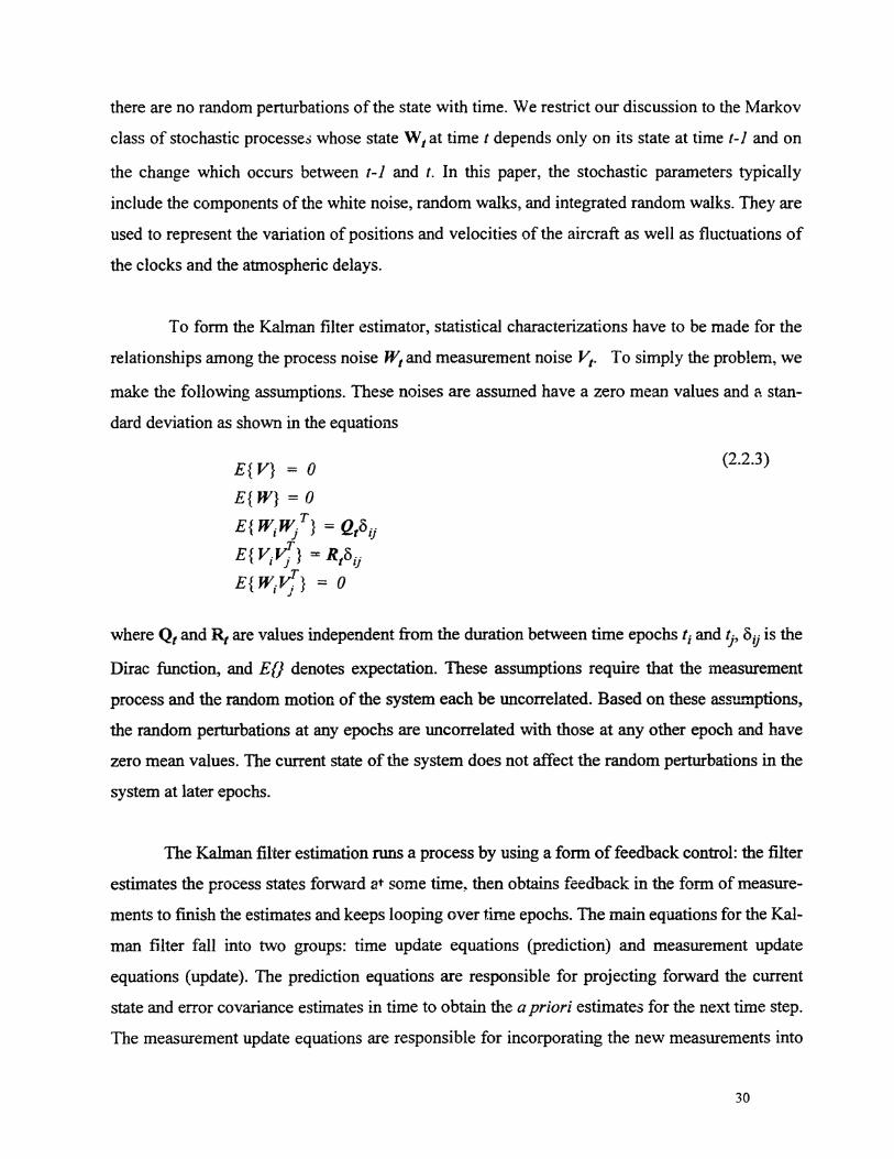
To form the Kalman filter estimator, statistical characterizations have to be made for the

relationships among the process noise WI and measurement noise Vt. To simply the problem, we

make the following assumptions. These noises are assurned have a zero mean values and a stan­

dard deviation as shown in the equations

E{ V} = 0

E{ W} = 0T

E{ Wi"} } = QtOij

E{ V.V:} :r; Rto ..I J I)

TE{ Wi~} = 0

(2.2.3)

where Qt and R t are values independent from the duration between time epochs Ii and ~, oij is the

Dirac function, and E{} denotes expectation. These assumptions require that the measurement

process and the random motion of the system each be uncorrelated. Based on these asSlL'llptiOns,

the random perturbations at any epochs are uncorrelated with those at any other epoch and have

zero mean values. The current state of the system does not affect the random perturbations in the

system at later epochs.

The Kalman filter estimation runs a process by using a fonn of feedback control: the filter

estimates the process states forward at some time, then obtains feedback in the form of measure­

ments to finish the estimates and keeps looping over time epochs. The main equations for the Kal­

man filter fall into two groups: time update equations (prediction) and measurement update

equations (update). The prediction equations are responsible for projecting forward the current

state and error covariance estimates in time to obtain the a priori estimates for the next time step.

The measurement update equations are responsible for incorporating the new measurements into

30

the a priori estimates to obtain the improved a posteriori estimates. The whole procedure of Kal­

man filtering could consist of three parts: initialization, prediction, and update as in Figure 2.1

A. Initialization Step

We consider the d)'narnic system to commence at the initial epoch 10. We assume its state

vector is Xo and its covariance matlix po. XG, Po is knowra at to as

(2.2.4)

00 is the m-dimensional known ·vector. and Po is an m by m symmetric matrix.

B. Prediction Step

The prediction step could be thought of as a time update equation. A dynamic propagation

relationship like equation (2.2.2) allows us to make a forward prediction from any epoch 1-1 to t.

The time dependent state vector Xtlt-1 is projected with its dynamic state transition matrix $t,t-1

for epoch t from its values Xt-1 at epoch 1-1

(2.2.5)

Using the law of covariance propagation appeared to Equation (2.2.2) with the assumptions in

equation {2.2.3}, the predicted covariance Ptlt-l for Xtlt-1 is

(2.2.6)

The prediction step provides the best "guess" for the next time and its associated as variance

based on the available infonnation in current time t. The covariance is composed of two parts, the

state Wlcertainty and the stochastic noise contribution during time between epochs 1-1 and t.

31

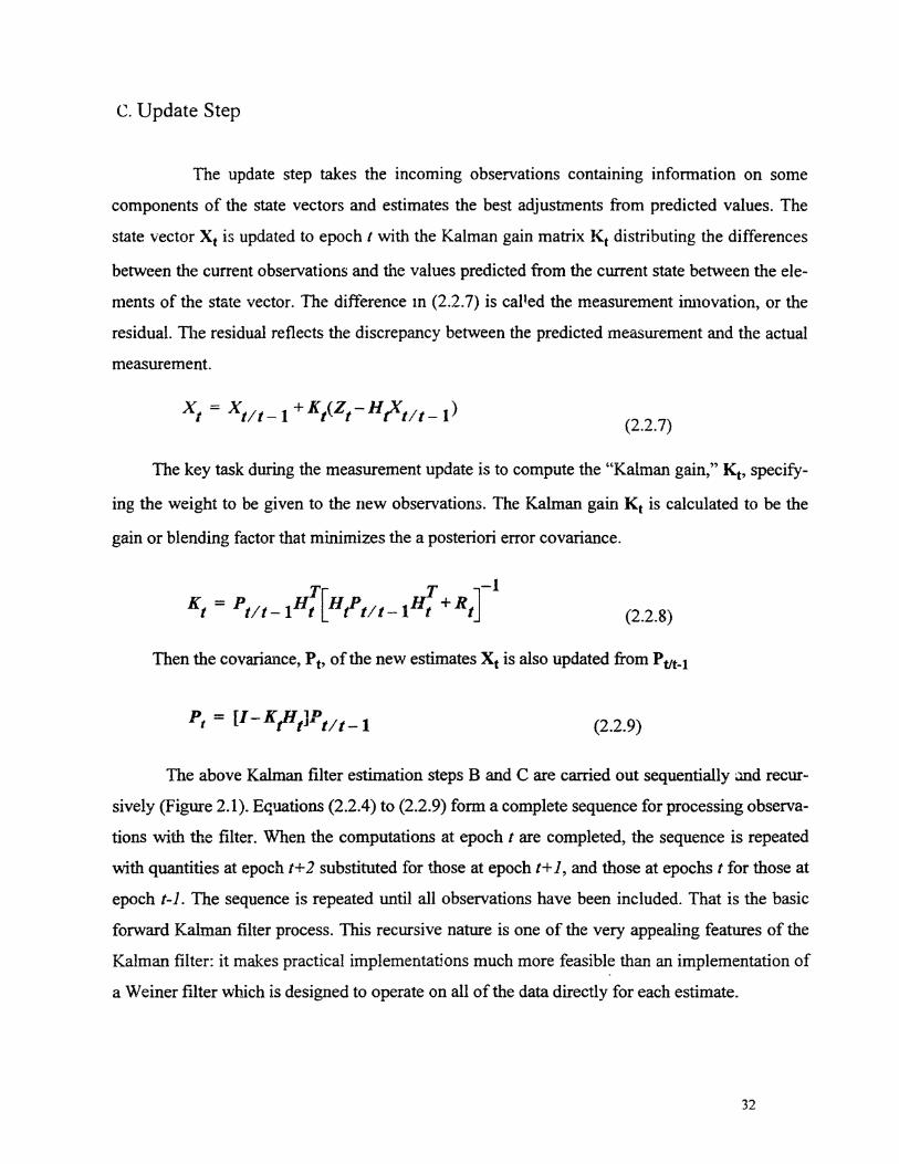
c. Update Step

The update step takes the incoming observations containing infonnation on sOlne

components of the state vectors and estimates the best adjustments from predicted values. The

state vector Xt is updated to epoch / with the Kalman gain matrix K t distributing the differences

between the current observations and the values predicted from the current state between the ele­

ments of the state vector. The difference In (2.2.7) is called the measurement imlovation, or the

residual. Tile residual reflects the discrepancy between the predicted measurement and the actual

measurement.

(2.2.7)

The key task during the measurement update is to compute the "Kalman gain," K t , specify­

ing the weight to be given to the Ilew observations. The Kalman gain K t is calculated to be the

gain or blending factor that minimizes the a posteriori error covariance.

(2.2.8)

Then the covariance, P t , of the new estimates X t is also updated from Ptlt-l

(2.2.9)

The above Kalman filter estimation steps B and C are carried out sequentially JDd recur­

sively (Figure 2.1). Equations (2.2.4) to (2.2.9) form a complete sequence for processing observa­

tions with the filter. When the computations at epoch t are completed, the sequence is repeated

with quantities at epoch t+2 substituted for those at epoch t+1, and those at epochs t for those at

epoch 1-1. The sequence is repeated until all observations have been included. That is the basic

forward Kalman filter process. This recursive nature is one of the very appealing features of the

Kalman filter: it makes practical implementations much more feasible than an implementation of

a Weiner filter which is designed to operate on all of the data directly for each estimate.

32

There are three types of applications of the Kalman filter for data analysis: sITloothing,

filtering, and predicting representing the process of providing solutions for past, current, and

future epochs, respectively. Most of the applications in this thesis are filtering; i.e. providing

solutions for the current epoch. For smoothing, the forward process is not complete because the

estimates do not yet incorporated data from epoch t+J forward. A backward process helps the

smoothing but is not necessary in the filtering. For details of the application of a backward

Kalman filter for geodetic measuremen~ readers call refer to Herring et aI, [1990]. Strictly, the

trajectory detennination would be better if it comes from a smoothing processing. We use a

single forward processing, however, which is much simpler for design. The use of a forward­

only process is also based on other two considerations: one is that the potential future application

of this software for real time use demands a design as a forward process; the other is that, with

current precise phase measurements and robust Kalman filter process design, the results of

forward processing is smooth and accurate enough without further backward smoothing.

2.3 GPS Observations

The fundamental measurements recorded by a GPS receiver are the differences in time

or phase between the signals from GPS satellites and similar signals generated by the receiver.

GPS signals are transmitted at two frequencies: Ll (1575.42 MHz) and L2 (1227.60 MHz).

Several different combinations of GPS observations are used in this thesis for different purposes.

We discuss the code pseudorange, carrier phase, and their useful linear combinations in this

section.

2.3.1 Pseudorange Observations

The pseudoranges between the satellite and the receiver are derived from the difference in

reception time and transmission time of an encoded satellite signal. Up to two pseudorandom

noise (PRN) codes are modulated onto the two base carriers (L1 and L2). The L I signal is

modulated with a CIA (Course Acquisition) code and a higher rate P (Precision) code. The L2

33

signal does not have CIA code modulated on its carrier. When anti-spoofirag is active (as it is for

data analyzed here), the P code is further modulated with a code called the W code. The product

of the P and W code is the Y code. The range provided by code tracking is called "pseudorange"

because the value includes not only the true range from the satellite to the receiver but also the

clock biases of satellite and receiver. Here, we denote by Is the time given by the satellite clock

at the transmission time and by tr the time given by the receiver clock at signal reception. The

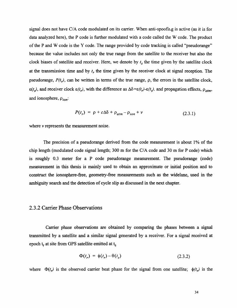
pseudorange, P(tr), can be written in tenns of the true range, p, the errors in the satellite clock,

E(tJ, and receiver clock E(tr), with the difference as ~8=E(tr)-f,(IJ, and propagation effects, Palm'

and ionosphere, Pion:

P(tr ) = p + c~o + Palm - Pion + V

where v represents the measurement noise.

(2.3.1 )

The precision of a pseudorange derived from the code measurement is about 1% of the

chip length (modulated code signal length; 300 m for the CIA code and 30 m for P code) which

is roughly 0.3 meter for a P code pseudorange measurement. The pseudorange (code)

measurement in this thesis is mainly used to obtain an approximate or initial position and to

construct the ionosphere-free, geometry-free measurements such as the widelane, used in the

ambiguity search and the detection ofcycle slip as discussed in the next chapter.

2.3.2 Carrier Phase Observations

Carrier phase observations are obtained by comparing the phases between a signal

transmitted by a satellite and a similar signal generated by a receiver. For a signal received at

epoch !r at site from GPS satellite emitted at ts

(2.3.2)

where c.I>(trJ is the observed carrier beat phase for the signal from one satellite; ~(tr) is the

34

carrier phase received from the satellite; and e(rJ is the phase of the local oscillator of the GPS

receiver.

Like the code measurement equation, equation (2.3.2) can be further written as

(2.3.3)

where the wavelength A is for L1 or L2; the <1>0 represents the initial bias in each phase

measurement.

The precision of GPS pllase observations is normally about 1% of the wavelength. One

cycle of carrier phase is about 19 em for L1 frequency and 24 em for L2 frequency. The phase

observation at LI, L2 or its linear combination L3 (see Section 2.3.4) are used for em-level

precision positioning. The software and algorithm developed here, however, are capable of

dealing with either pseudo-range data, or the carrier phase data.

2.3.3 Single and Double Differencing

In local kinematic surveys, normally two GPS receivers are used: one is on the moving

vehicle, the other is on the fIXed station with known position. In analyzing data, we fIrst fOIm the

difference of observations from the same GPS satellite in the two receivers. The difference

between receivers is conventionally referred to as "receiver single difference"; it may be written

for at the L1 and L2 frequencies as

(2.3.4)

where Al and Atare the wavelengths ofLI and L2. The only difference between equations 2.3.3

35

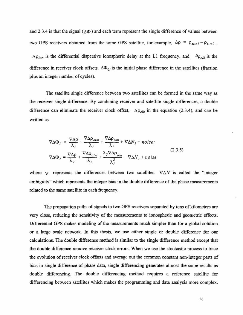
and 2.3.4 is that the signal (~<1» and each term represent the single difference of values between

two GPS receivers obtained from the same GPS satellite, for example, 6.p = Pslle I - Pslte2 .

~P;on is the differential dispersive ionospheric delay at the LI frequency, and tJpclk is the

difference in receiver clock offsets. ~<I>Oi is the initial phase difference in the satellites (fraction

plus a.." integer number of cycles).

The satellite single difference between two satellites can be formed in the same way as

the receiver single difference~ By combining receiver and satellite single differences, a doubJe

difference can eliminate the receiver clock offset, tiPclk in the equation (2.3.4), and can be

written as

DA V~p V~p.VL1p + aIm + Ion + t"7A AT + . .T A A v U1.Y J nOIse,

J J I

rlA \7~p A V8p.n A rh =~ + atm + 2 Ion + n A 'AT + .ViJ.'-V2 A A 2 VUlv2 nOise

2 2 AJ

(2.3.5)

where V represents the differences between two satellites. \78N is called the "integer

ambiguity" which represents the integer bias in the double difference of the phase measurements

related to the same satellite in each frequency.

The propagation paths of signals to two GPS receivers separated by tens of kilometers are

very close, reducing the sensitivity of the measurements to ionospheric and geometric effects.

Differential GPS makes modeling of the measurements much simpler than for a global solution

or a large scale network. In this thesis, we use either single or double difference for our

calculations. The double difference metb.od is similar to the single difference method except that

the double difference remove receiver clock errors. When we use the stochastic process to trace

the evolution of receiver clock offsets and average out the common constant non-integer parts of

bias in single difference of phase data, single differencing generates almost the same results as

double differencing. The double differencing method requires a reference satellite for

differencing between satellites which makes the programming and data analysis more complex.

36

The residual infonnation of single difference can also help us to identify the problematic

observations with specific satellite. The double difference of carrier phase measurements is used

in the ambiguit)l search which will be introduced in Chapter 3. In the analysis of Long Valley

measurements in Chapter 4, we will use single difference of carrier phase most of time.

2~3.4 Linear Combinations of Observations

We use several linear combinations of the original carner phase and/or code

measurements during the data analyses. Those combinations are the ionosphere-free linear

combination of canier phase (L3), the extrawidelane geometry-free ]in°.a~ observation (L4), the

widelane observation (L5) and the ionosphere-free and geometry-free combination of carrier

phase and code observations (L6). (We adopt the nominative of [Beutler et. aI, 1996]; other

investigators [king and Bock, 1998] have used LC for L3 and LG for L4). We discuss them in

this section. In the following discussion, L} and L2 represents the phase observations in cycles

(appropriate to the frequencies), and PI and P2 represent the code measurements in meters at the

LI and L2 frequencies, respectively~ For simplicity, we use the following symbols for the phase

measurement at L1 and L2.

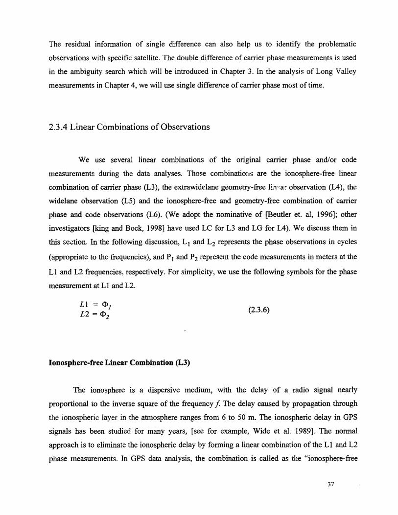
LI = <1»

L2 = <1>2

Ionosphere-free Linear Combination (L3)

(2.3.6)

The ionosphere is a dispersive medium, with the delay of a radio signal nearly

proportional to the inverse square of the frequency f The delay caused by propagation through

the ionospheric layer in the atmosphere ranges from 6 to 50 m. The ionospheric delay in GPS

signals has been studied for many years, [see for example, Wide et aI. 1989]. The normal

approach is to eliminate the ionospheric delay by forming a linear combination of the L 1 and L2

phase measurements. In GPS data analysis, the combination is called as tIle "ionosphere-free

37

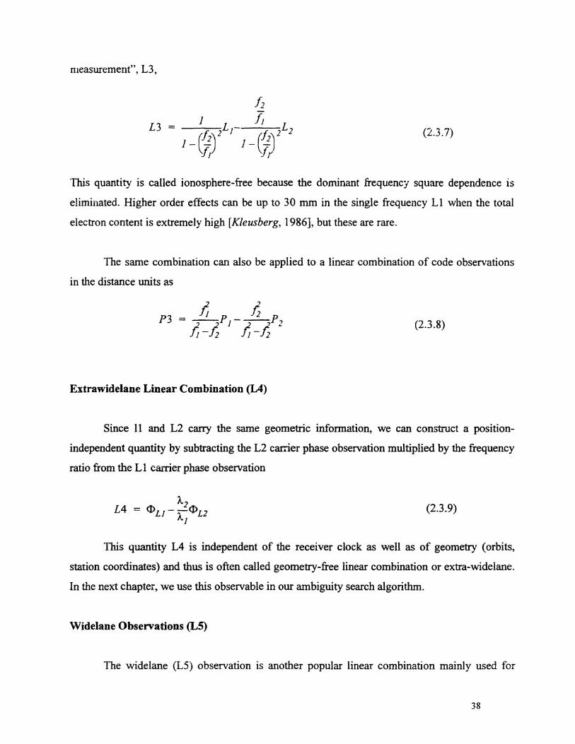
rrleasurement", L3,

(2.3.7)

This quantity is called ionosphere-free because the dominant frequency square dependence is

elimillated. Higher order effects can be up to 30 mm in the single frequency L1 wIlen the total

electron content is extremely high [Kleusberg, 1986], but these are rare.

The same combination can also be applied to a linear combination of code observations

in the distance units as

(2.3.8)

Extrawidelane Linear Combination (L4)

Since II and L2 carry the same geometric information, we can construct a position­

independent quantity by subtracting the L2 carrier phase observation multiplied by the frequency

ratio from the L1 carrier phase observation

(2.3.9)

This quantity L4 is independent of the receiver clock as well as of geometry (orbits,

station coordinates) and thus is often called geometry-free linear combination or extra-widelane.

In the next chapter, we use this observable in our ambiguity search algorithm.

Widelane Observations (L5)

The widelane (L5) observation is another popular linear combination mainly used for

38

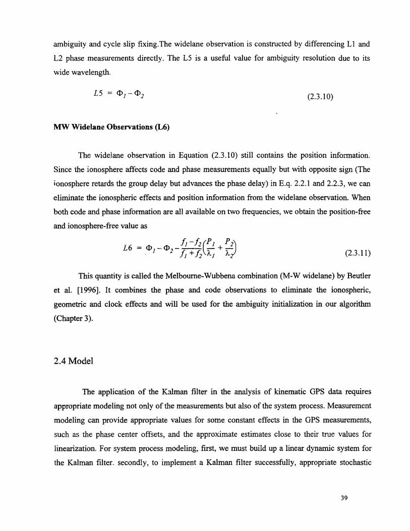
ambiguity aI1d cycle slip fixing.The widelane observation is constructed by differencing LI and

L2 phase measurements directly. The L5 is a useful value for ambiguity resolution due to its

wide wavelength.

(2.3.10)

MW Widelane Observations (L6)

TIle widelane observation in Equation (2.3.10) still contains the position information.

Since the ionosphere affects code and phase measurements equally but with opposite sign (The

ionosphere retards the group delay but advances the phase delay) in E.q. 2.2.1 and 2.2.3, we can

eliminate the ionospheric effects and position infonnation from the widelane observation. When

both code and phase information are all a.vailable on two frequencies, \ve obtain the position-free

and ionosphere-free value as

(2.3.11)

This quantity is called the Melbourne-Wubbena combination (M-W widelane) by Beutler

et al. (1996]. It combines the phase and code observations to eliminate the ionospheric,

geometric and clock effects and will be used for the ambiguity irjtialization in our algorithm

(Chapter 3).

2.4 Model

The application of the Kalman filter in the analysis of kinematic GPS data requires

appropriate modeling not only of tI'1e measurements but also of the system process. Measurement

modeling can provide appropriate values for some constant effects in the GPS measurements,

such as the phase center offsets, and the approximate estimates close to their trlIe values for

linearization. For system process modeling, first, we must build up a linear dynamic system for

the Kalman filter. secondly, to implement a Kalman filter successfully, appropriate stochastic

39

processes must be chosen to represent the behavior of parametric models. In this section, we

discuss the use of both measurement and kinematic process modeling clock offset, atmospheric

delay, and position changes.

The parameters used in a Kalman filter can be considered as stochastic ones. In a

dynamic system, the statistical models adopted to represent a stochastic parameter sllould depend

on the ph)TSics of the noise-generating process. Most of the underlying physics, however, is not

\\'ell lmderstood~ lbe implementation of the ideal stochastic process sometimes yields a

cumbersome solution so that an exact representation is often not practicable, if not prohibitive.

Based on the experience of using the Kalman filter in other geodetic meastlfements such as VLBI

[Herring et aI., 1990], we adopt three types of stochastic processes to represent the variations of

parameters: white noise, random walk, and integrated random walk.

Depending on the type of data used, pseudorange or carrier phase, the GPS measurement

equation is either equation (2.3.1) or (2.3.3). If the ambiguity N is taken out of the carrier phase

measurement equation (2.3.3), there is little difference in the treatment of the phase and range

measurements. In the following discussion, we develop the state expression for both phase and

range data, and leave the ambiguity solution until the next chapter.

The improvement of GPS techniques has helped the use of the kinematic model in the

Kalman filter algorithm. In contrast to a pure dynamic system, the solution of a kinematic system

puts weight more heavily on the current measurements than on the past-time information. To

obtain a reliable solution from differential GPS measurements at one epoch, at least four

common satellites should be measurement from both GPS receivers. In our experiment,

normally, there are five to eight satellites available for both the receivers on the ground and on

the aircraft, although at times, the satellite availability does drop to four. The number of available

satellites depends on the distance of the aircraft from the base station as well as on other factors.

To keep a robust solution even in a satellite constellation with fewer satellites, we limit the

number ofparameters in our equations. With the differential measurements, the parameters in the

observation models are the unknown position of the target, the receiver clock offset, and the

atmospheric model.

40

In tile state equations, the state vector Xt contains the position information PI (both

position and velocity, or position only), the clock difference effect c/),0t, and the zenith delay

adjustment Dt representing the difference in atmospheric delay between the fixed and moving

receivers.

The stochastic process Inatrix is

W=t(2.4.2)

with coefficient matrix

I p 0 0r =t 0 I 0

001(2.4.3)

The associated covariance matrix of the process noise is

The meEsurement matrix is

the state transition matrix is

(2.4.4)

(2.4.5)

41

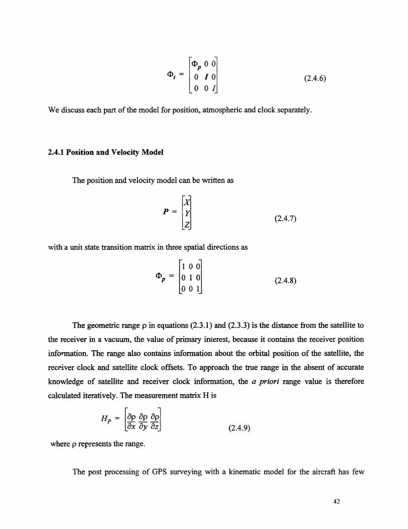
(2.4.6)

We discuss each part of the model for position, atmospheric and clock separately.

2.4.1 Position and Velocity Model

The position and velocity model can be written as

P = Y

Z

with a unit state transition matrix in three spatial directions as

100<I>p = 0 1 0

001

(2.4.7)

(2.4.8)

The geometric range p in equations (2.3.1) and (2.3.3) is the distance from the satellite to

the receiver in a vacuum, the value of primary interest, because it contains the receiver position

infoTIllation. The range also contains information about the orbital position of the satellite, the

receiver clock and satellite clock offsets. To approach the true range in the absent of accurate

knowledge of satellite and receiver clock information, the a priori range value is therefore

calculated iteratively. The measurement matrix H is

(2.4.9)

where p represents the range.

The post processing of GPS surveying with a kinematic model for the aircraft has few

42

constraints on lt~ ~'ariation of acceleration and velocity. Thus the use of a stochastic process to

model position depends on the behavior of the velocity of the aircraft during the entire flight.

Normally a combination of white noise, random walk (integrated white noise) and integrated

random walk can simulate most of process noises.. Based on the navigation application of a

Kalman filter by other instigators and several tests we had run with different combination of

components from three standard processing noises, we use a white noise for the velocity

stochastic model for Long Valley analysis. The position therefore behaves as a random walk..

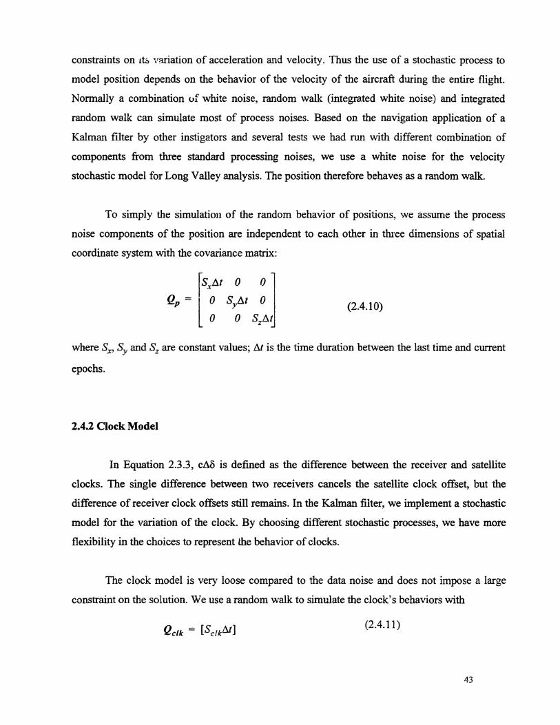
To simply the simulatioll of the random behavior of positions, we assume the process

noise components of the position are independent to each other in three dimensions of spatial

coordinate system with the covariance matrix:

fSxAt 0 0

Qp = l 0 Sylit 0

o 0 Sz~t

(2.4 .. 10)

where Sx, Sy and Sz are constant values; /).t is the time duration between the last time and current

epochs.

2.4.2 Clock Model

In Equation 2.3.3, cL\o is defined as the difference between the receiver and satellite

clocks. The single difference between two receivers cancels the satellite clock offset, but the

difference of receiver clock offsets still remains. In the Kalman filter, we implement a stochastic

model for the variation of the clock. By choosing different stochastic processes, we have more

flexibility in the choices to represent the behavior of clocks.

The clock model is very loose compared to the data noise and does not impose a large

constraint on the solution. We use a random walk to simulate the clock's behaviors with

(2.4.11)

43

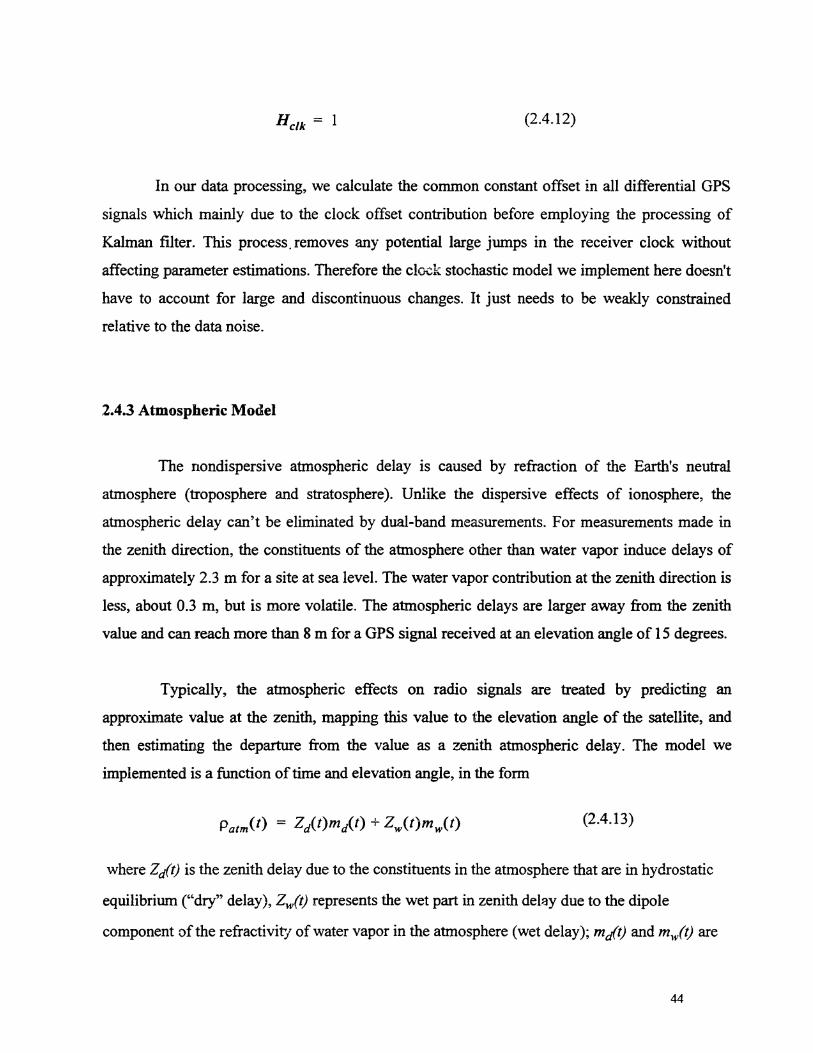
(2.4.12)

In our data processing, we calculate the common constant offset in all differential GPS

signals which mainly due to the clock offset contribution before employing the processing of

Kalman filter. This process. removes any potential large jumps in the receiver clock without

affecting parameter estimations. Therefore the clock stochastic model we implement here doesn't

have to account for large and discontinuous changes. It just needs to be weakly constrained

relative to the data noise.

2.4.3 Atmospheric Model

The nondispersive atmospheric delay is caused by refraction of the Earth's neutral

atmosphere (troposphere and stratosphere). Unlike the dispersive effects of ionosphere, the

atmospheric delay can't be eliminated by dual-band measurements. For measurements made in

the zenith direction, the constituents of the atmosphere other than water vapor induce delays of

approximately 2.3 m for a site at sea level. The water vapor contribution at the zenith direction is

less, about 0.3 m, but is more volatile~ The atmospheric delays are larger away from the zenith

value and can reach more than 8 m for a GPS signal received at an elevation angle of 15 degrees.

Typically, the atmospheric effects on radio signals are treated by predicting an

approximate value at the zenith, mapping this value to the elevation angle of the satellite, and

then estimating the departure from the value as a zenith atmospheric delay. The model we

implemented is a function of time and elevation angle, in the fonn

(2.4.13)

where Zeit) is the zenith delay due to the constituents in the atmosphere that are in hydrostatic

equilibrium ("dry" delay), Zw(t) represents the wet part in zenith delay due to the dipole

component of the refractivirj of water vapor in the atmosphere (wet delay); melt) and m,V(t) are

44

the mapping functions for hydrostatic and wet delay respectively [Davis et a/., 1985, Herring

1992]. The mapping function can be Marini's [Marini, 1974], CfA-2.2 [Davis et a/., 1985], MTT

function [Herring, 1992], or NMF function [Niell, 1996]. We provide the different mapping

functions in Appendix A.

The model values of tropospheric zenith delays Zeit) and Zw(t) are calculated with a

model from Saastamoinen [1972] model with typical and constant meteorological conditions at

sea level with pressure 1013.25 mb, temperature 20°C and relative humidity 50%. The pressure

at the height of the receiver is extrapolated by assuming hydrostatic equilibrium [Davis, 1986]

and a lapse rate of -6.5° C/km [Holton, 1979]. In the flight test, the altitude of the aircraft could

vary from zero to a few kilometers. The extrapolated zenith delay value is still approximate, so

an atmospheric delay correction is needed when the atmospheric delay has large variations or the

records of the meteorologic measurements are not correct..

The uncorrected atmospheric delay in (2.4.12) is modeled as a random walk in the zenith

direction and the dry mapping function is used to map the zenith value to the elevation angle of

viewing. The selection of the stochastic variance for zenith delay is a little difficult for

kinematic GPS surveying because most of models developed for static ground sites but the

aircraft moves in a zone covered 10 kIn vertically and 100 kmhorizontally. A thorough study of

the statistical fluctuations of water vapor under the assumptions of Kolmogorov turbulence

theory by Treu17aft and Lanyi [1987] shows that the structure function for the propagation delay

in the zenith direction could be similar to that of random walk process in a limited frequency

domain. This conclusion leads to the successful use of a random walk in VLBI measurements

[Herring et al., 1990]. The stochastic model is applied just to the moving receiver in the analysis

here although our software can handle the atmospheric estimations on both fixed and moving

receivers. Our test shows that the variation of atmospheric delay in zenith is limited to under 1 to

2 centimeter in most experiments.

The process noise for the atmospheric correction is

(2.4.13)

45

(2.4.14)

where Satm in unit of m2/s and Md is the dry mapping function. The mapping function we used in

our algorithm is the MTT dry mapping function [Herring, et al., 1992].

The precise modeling is important to keep t.he Kalman filter processing smoothly. To

obtain high precise position estimates from the phase data, however, we still have to solve the

ambiguity problem at flrs~ which is addressed at the next chapter.

46

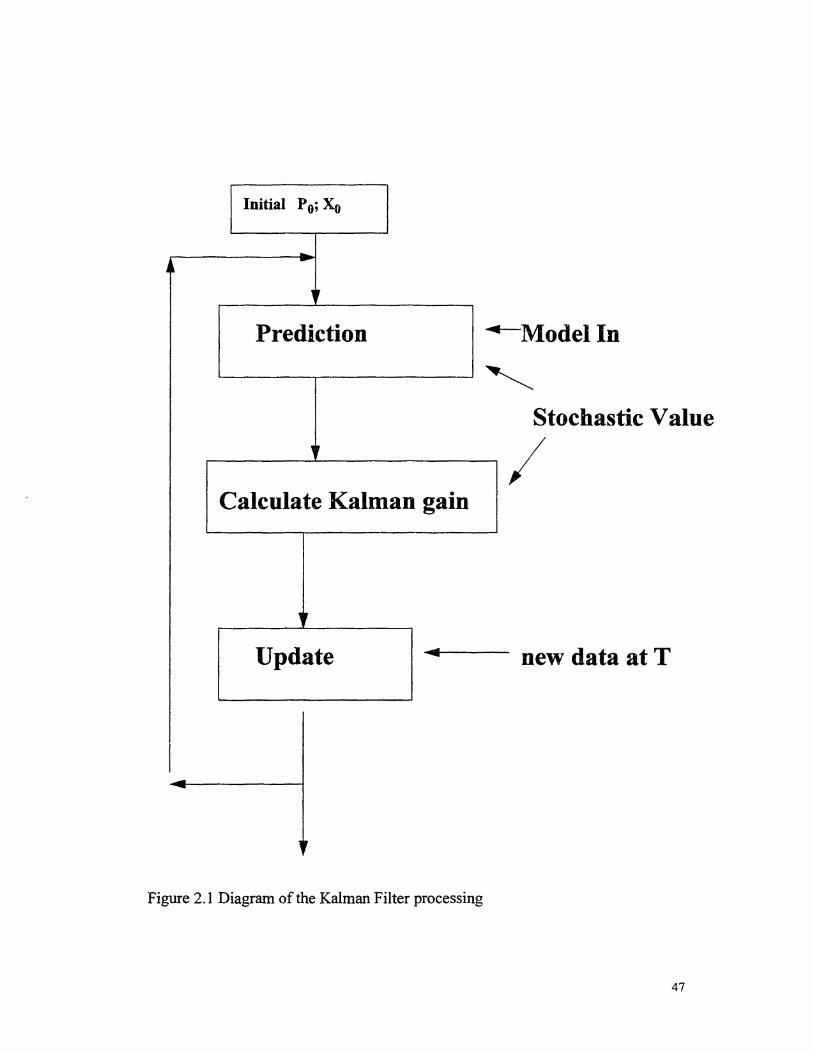
Initial Po; Xo

.....

"Prediction ""'-Modelln

Stochastic Value~ ',---r ----, /

Calculate Kalman gain

"Update

Figure 2.1 Diagram of the Kalman Filter processing

new data afT

47

Reference

Beutler G., E. Brockmann, S. Fratlkhauser, W. Gurtner, J. Johnson, L. Mervart, M. Rothacher, S.

Schaer, T. Springer, R. Weber, Bernese GPS Software, Version 4.0, Eds. by L. Mervart

and M Rothacher, Astronomic institute, Univ. ofBerne, 1996

Brown, R.G. and Y.C. Hwang, Introduction to Random Signals and Applied Kalman Filtering,

Second edition, John Wiley & Sons Gelb, A. (ed), 1974, Applied Optimal Estimation, MIT

press, Cambridge Mass, pp. 374, 1992.

Cohn, S., M. Ghil, and E. Isaacson, Optimal Interpolation and the Kalman Filter, Proceedings of

the Fifth Conference on Numerical Weather Prediction, Monterey California, American

Meteorological Society, Boston Mass., 36 - 42, 1981

Davis, J,L., Atmospheric propagation effects on radio Interferometry, Ph. D. Thesis, MIT,

Cambridge, MA, 1986

Davis, J. L, T. A. Herring, and I. I. Shapiro, Effects of atmospheric modeling error on

determinations of baseline vectors from VLBI, J. Geophys. Res., 96, 643-650, 1991.

Gelb, A., Applied Optimal Estimation, 274 pp., MIT Press, Cambridge, Mass., 1974.

Genrich, J. F. and J. B. Minster, Ship navigation for geophysical applications using kalman­

filtered GPS fixes, Geophysics, 56,1961-1970, 1991.

Herring, T. A., The precision and accuracy of intercontinental distance determinations using

radio Interferometry, Ph. D. Thesis, MI.T., Cambridge, MA, 1983.

Herring, T. A., J. L. Davis and I. I. Shapiro, Geodesy by radio interferometry: The application of

Kalman filtering to the analysis ofVLBI data, J Geophys. Res., 95, 12561-12581,1990.

Herring, T. A., modeling atmospheric delays in the analysis of space geodetic data, in Refraction

of trans-atmospheric Signals in Geodesy, eds. J. C. Munck and T. A. Spoelstra,

Netherlands Geodetic Commission Publications in Geodesy, 36,157- 36,164,1992.

Holton, I, R., An introduction to dynamic meteorology, International Geophysics series, Vol. 16,

Academic Press, London, 1972.

Ifadis, I. I., The atmospheric delay of radio waves: Modeling the elevation dependence on a

global scale, Technical Report #38L, Chalmers University of Technology, G6teborg,

48

Sweden, 1986

Jacobs~ O.L.R, Introduction to Control Theory, second edition, Oxford University Press, 1993.

Julier, S. J., J. K. Uhlmann, and H~ F. Durrant-Whyte, A New Approach for Filtering Nonlinear

Systems. Proceedings of the 1995 American Control Conference, Seattle, Washington,

1628-1632, 1995.

Lewis, R.,Optimal Estimation with an Introduction to Stochastic Control Theory, John Wiley &

Sons, Inc., 1986.

Liebert, P.B., An introduction to optimal estimation, Addison-Wesley, Reading, Mass., 273 pp.,

1967.

Kalman, R.E., and Buey, R.S., New results ill Linear Filtering and Prediction Theory, J. Basic

Eng., 95-108, 1961.

Kalman, R.E., A new Approach to Linear Filtering and Prediction Problems, J. Basic Eng.,

March, 35-46, 1960.

Kleusberg, A., ionospheric propagation effects in geodetic relative GPS positioning, Man. Geo.,

11, 256-261, 1986.

King, R. W., Documentation for the MIT GPS Analysis Software: GAMIT, Mass. Institute of

Technology, 1997

Marini, J. W. and Murray, C. W., Correction of laser range tracking data for atmospheric

refraction at elevations above 10 degrees, NASA report X-591-73-351, Goddard Space

Flight Center, 1973.

Marini, J. W, Correction of satellite tracking data for an arbitrary atmospheric profile, Radio

Science, 7, 223-231, 1972.

Niell, A. E., Vertical change and atmosphere correction in VLBI, in Proceedings of the AGU

~hapmanConference orl Geodetic VLBI: Monitoring Global Change, NOAA Tech. Rep.

NOS 137 NGS 49,428-436, U.S. Dept. ofCommer., Rockville, Md., 1991.

Niell, A. E., Global mapping functions for the atmosphere delay at radio wavelengths, J.

Geophys. Res., 101, B2, 3227-3246, 1996.

Saastamoinen, Contribution to the theory of atmospheric refraction. Bulletin Geodesique, Vol

107, 13-34,1972

Shinbert, M., Optimization of Time-varying linear Systems with Nonstationary Inputs, Trans.

ASME, 80, 457-462, 1958

49

Truehaft, R. N., & G. E. Lanyi, The effect of the dyna..llic wet tropospheric radio interferometric

measurements, Radio Sci., 22,251-265,1987.

Wild D., Beutler G., Gurtrler W. and Rothacher M, Estimating the ionosphere using one or more

dual frequency GPS receivers. In: Proceedings of the Fifth International Geodetic

Symposium on Satellite Positioning, Las Cruces, New Mexico, March 13-17, Vol. 2,724­

736, 1989.

50

Chapter 3 Phase Ambiguity Resolution Strategy

3.1 Introduction

To meet the precision requirement ofcentimeter for the aircraft positioning in this experi­

ment, we must use GPS carrier phase observations for accurate aircraft kinematic positioning.

As indicated in the Chapter 2, the observed quantity of phase is the beat phase (i.e. the difference

between the satellite-transmitted carrier and a receiver generated replica signal). When a receiver

is turned on, the fractional beat phase is observed and an integer counter is initialized. During

GPS signal tracking, the counter increments by one cycle whenever the fractional phase changes

from 21t to o. Therefore the accumulated phase recorded at a given epoch is the sum of the frac­

tional phase observable signal and a phase bias. The bias contains a non-integer value plus the

number of the unobserved full cycles of the phase observation, an inherent cycle ambiguity N of

carrier phase measurement.

For geodetic measurements, time-varying phase observable contains two parts of informa­

tion: interesting (i.e. position, time) and uninteresting (i.e. receiver clock drift and phase bias)

components. For the correct use ofGPS carry phase, the key is to eliminate the uninteresting parts

from the observables. In a local GPS measuremellt, the differential technique generally cancels

out most of model errors from the atmospheric, ionospheric and tide errors. Double differencing

removes both satellite and receiver clock offsets. Single differencing removes satellite clock off­

sets and the remain receiver clock offset can also easily be estimated as a common value for all

satellites. Unlike other factors which have common sources, the phase bias is receiver channel

dependent. In GPS receiver, each channel initializes its own counter for one satellite so the phase

biases can't be canceled by differencing and modeling. Resolving unknown phase bias becomes a

fundamental requirement for accurate em-level GPS aircraft kinematic positioning.

Theoretically, the phase bias of one channel in a receiver (one-way observation) is defmed

as a combination of cycle ambiguity N and a non-integer part. When double differences are

fanned, however, the non-integer part of the bias due t the unknown initial phase of the transmit-

51

ting and receiver clocks are eliminated. Hence we used double difference for the ambiguity reso­

lution. The re:nlatmng integer part of bias is generally called ambiguity. For single differenced

phase observables, the non-integer part of their biases can be calculated as a constant non-integer

bias at the beginning of data processing; the remaining ambiguities are the same as the integer

ambiguities in their double differences.

Without the exact determination of the integer ambiguity, precise positioning at the centi­

meter level using GPS phase observations cannot be achieved. It is easy to see that a mis-detenni­

nation ofone cycle ofambiguity could result in a few to tens ofcentimeter shift in the estimates of

GPS position. Moreover, ambiguity resolution is more crucial in the kinematic surveying than in

the static one. In static GPS analysis, we can separate the ambiguities from the receiver's fixed

position by the geometric changes of satellites in a long time observation. In kinematic GPS sur­

veying, the occupation of receiver in one location is short, even varies from epoch by epoch. The

ambiguities are high-correlated with positions. Hence, the phase ambiguities must be correctly

resolved beforehand in order to convert the phase observations into the precise ranges to the GPS

satellites for accurate positioning.

Ambiguity resolution is necessary at three occasions: the beginning of the session (initial

ambiguity), cycle slip occurrences, and the rising of a new satellite to be included in GPS analy­

sis. The initial integer number N of cycles between the satellite and the receiver is typically

unknown at the beginning of the receiver signal cOWlting. The receiver may reset its initial ambi­

guities each time that it is turned on or sets initial numbers for a new satellite in one channel. This

phase ambiguity N remains constant as long as no loss of signal lock occurS$ Discontinuance may

occur during an experiment when, for example, the receiver loses lock of signal when the satellite

signal is blocked by some buildings or a wing of the aircraft during banking. In this event, the

integer counter is re-initialized, causing a jump in the instantaneous accumulated phase by an

integer number ofcycles. This jump is called a cycle slip and is restricted to phase measurements.

The greatest difficulty for the ambiguity resolution is how to extract the integer cycle

numbers from phase observations without the knowledge of precise position. The simpiest ambi­

guity resolution process is the direct use of the ambiguity-free pseudorange measurements for LI

52

and L2 to obtain estimates of position and ionospheric delay, then to determine the ambiguity

value [Blewitt, 1987]. The problem with the pseudorange measurement method is that the mea­

surement error from receiver noise and signal multipathing are high. The use of single-epoch data

can cause position errors around 1 meter, resulting in several or more cycle errors in ambiguities.

The widelane comblilation of phase observations, L5, is occasionally fonned to help the

ambiguity detennination because its long wavelength (86 cm) reduces the impact of position

errors on the ambiguity determination. The position-free difference between the associated code

and the carrier mea.c:;urements (L6) fonned. Their averages over a time period are rounded to the

nearest integer to obtain the ambiguities. However, the widelane (L6) still suffers the effects of

the multipath errors and pseudorange r~leasurementerrors and can have variation of 1-2 cycles.

In these geometric approaches to ambiguity determination, the unmodeled errors will

affect all estimated parameters. Many error sources affect the closeness of the estimated ambigu­

ities to their integer values. Some of these sources could be, but are not limited to, the unmodeled

errors in phase, varying atmospheric conditions, and sateilite orbital errors. The ionosphere may

also prevent a correct resolution ofall ambiguities for a long baseline. In static surveying, data are

collected over a long time span and used to smooth out the variation of unrrlodeled errors such as

the multipath, ionospheric, and tropospheric effects on the ambiguity selection. When multiple

stations are used, redundant baseline combinations between any two stations can also help for the

search of ambiguities. Such a strategy is very efficient in static GPS measurements. In the kine­

matic GPS mod, however, these methods suffer some limitations, especially when the static ini­

tialization stage is short or does not exist. The major disadvantage of these techniques is the

length of time needed to achieve the required accuracy. In kinematic surveying, the initial static

stage before one starts moving usually does not last very long, sometime maybe just a few min­

utes. In our experiment, the code range data do not have enough time to allow the position solu­

tions to approach the right position before the airplane takes off. Although such methods have

been used in kinematic surveyinb LHatch, 1986, Bender and Lorden, 1985; Melbourne, 1985,

Wubbena, 1989], they still require improvement in the accuracy of code measurements and the

error models of the atmosphere and ionosphere to be effective over a long baseline.

53

In st~tic differential GPS positioning, ambiguity resolution benefits from a significant

change in satellite geometry and averagiIlg of errors over the long observation time span. In kine­

matic positioning, such advantages vanish and make the ambiguity resolution much more diffi­

cult. Research has indicated that there is no reliable analytic way to obtain the ambiguity solution

based in single epoch data in general condition. Also the integer characteristics of ambiguities

make it hard to resolve ambiguities with other unknown parameters directly from measurements

by optimum estimation. Generally, search techniques are needed.

During the last 10 years, numerical studies have been conducted for the "on-the-fly" ambi­

guity resolution which does not depend on the geodetic positions. A number of fast ambiguity­

search techniques have been published. Among the techniques, we have, ambiguity mapping

function method [Remondi, 1992; Madar, 1992]; least squares ambiguity search techniques

[Hatch, 1990 and 1991; Lachapelle, 1992]; fast ambiguity resolution approach [Frei and Beutler,

1990]; optimal Cholesky decomposition algorithm [Lalzdau and Euler, 1992]; ambiguity trans­

form method [Teunissen, 1994 and 1995]; dual frequency method [Abidin et al., 1992 and Abidin,

1993]; integer nonlinear programming method [Wei and Schwarz, 1995] and others. These ambi­

guity resolution techniques have common aspects. They are all applied to the initial ambiguity

resolution and have some search strategy for the best ambiguity combination. The differences

among them are mainly on how to execute such a search strategy. The detailed introduction and

discussion for these methods could be very long and exhausting and we are not going to discuss

these techniques in detail in this thesis. The major differences between these techniques fall into

three categories: the data type or infonnation utilized for the ambiguity search, the search domain

and strategy, and the verification criterion. Without some means for classifying the algorithm

employed, it is virtually impossible to evaluate their relative merit.

Many ambiguity-search methods have been developed to improve the computational

speed of the ambiguity-search process. When high memory costs were high and CPU speed was

low, minimizing the computations was important for real time solutions, especially for single fre­

quency solutions which require a large number of ambiguity combinations for testing. However,

an algorithm which results in fewer computations does not reduce the time span needed for the

verification of the chosen ambiguities. In our case, the kinematic surveying for Long Valley

54

project is the post-time process, not the real time process. Thus the speed of computation for the

ambiguity solution which many authors have addressed, is not our greatest concern.

Most above methods are also developed under the fine test environment which implies the

ionospheric, atmospheric, multipathing effects are negligible. The applications of these method

normally limit the kinematic moving within 10 km for local GPS differential surveying.. In a 100

Ian horizontal and 10 Ian vertical scale region the aircraft was flying, some of these assumptions

are impracticable. It is not surprise that some of methods failed to generate promising results in

our initial trials. We feel the strong need to develop an ambiguity search algorithm for aircraft

positioning to be not only fast but also reliable -- having the capability to deal with complex envi­

ronmental conditions.

In this thesis, we will develop our own amJiguity strategy. One of our aims is to develop

an ambiguity resolution strategy that is reliable and unique regardless of ali test conditions. We

want to develop robust methods for dealing with "bad" data so that the maximum amount of

observables can be used for positioning. The other goal is to reduce time span needed for ambigu­

ity detennination. From our purpose, reducing the computation time is less important than mini­

mizing the time span of data that must be accumulated before the ambiguities can be resolved

reliably. Although our method is based on previous studies, we will not restrict ourselves to any

specific techniques that have been developed. In this chapter, we design two different and effi­

cient ways to deal with different ambiguity situations. \'.Te firstly developed a position-free ambi­

guity search technique used for ambiguity initialization and re-initialization. Then we develop a

fast method to check and fix the cycle slips during a flight and to estimate the ambiguities for new

satellites that rise during a flight.

55

3.2 Initial Ambiguity Search Strategy

3.2.1 utilization of Dual Frequency Information

For convenience, we rewrite the double difference equation (2.3.5) as (3.2.1) for two

frequency observations as

t"7A v~p V'l\p.t"'7Am = ~ + atm + Ion + t"7A AT + . .VU\V] Iv A A VUJ.Vj nOIse,

] 1 J

V A VLip A2 \7L\p .n A m = -=:..e + atm + zon + n A AT + ·v U'-V2 A, A 2 v LJ,1V 2 nOise

2 2 AJ

(3.2.1)

Ambiguity resolution on kinematic GPS measurements can he carried out in different

search dimensions. Generally there are two possible search spaces: the physical three­

dimensional position space (L\.ps in equation 3.2.1) and the multi-dimensional mathematical

integer ambiguity space (/iNs in equation 3.2.1). The position-space search is simple to

implement. It tests numerical positions in a 3D space centered on an initial position. The best

ambiguity candidates are chosen based on the position that has minimum sum of residuals for all

observations. The shortcoming of the position space search is that it is very time consuming and

the search result is highly dependent on the initial position precision and search step size. Either

a too large step size can miss the right position point or a too small step size can increase the

computing time cubically. Thus its application in kinematic posit:onin3 is lilnited. Most

approaches are performed on the ambiguity space (LiN).

More recent ambiguity searches use the ambiguity space, which does not have the step

size selection problem. Generally the best way to estimate ambiguities is to estimate them

simultaneously with other parameters from the phase measurements directly. Assuming a bias­

free noise distributiorl, the integer ambiguities are determined by minimizing the a posteriori

error variance when all ambiguity integers, position parameters, and other model parameters

have been estimated. "The greatest complication comes from the integer constraint, which violates

the general rules of minimum residual swn if the least square method is applied directly with

56

equation (2.3.1). Due to this constraint, there is no unique analytical solution for the integer

ambiguity [Wei & Schwarz, 1995]. Therefore the influence of individual integer combinations on

the total error residual has to be computed separately and a search technique is necessary.

The use of double differences ~f the phase observations poses another problem. The

double differencing eliminates most common error sources such as receiver clock offset) which

is favorable for anlbiguity determination, but suffers a disadvantage in the statistically high

correlation between estimated ambiguities. SrJme strategies have been developed such as the

ambiguity transform method to decorrelate the ambiguities [Teunissen, 1994 and 1995].

Ho,vever, there is no reliable transfonn matrix developed for all circwnstances right now.

Although the defmition and construction of the ambiguity search are different for

different search methods, the core of the search techniques is the same: how to utilize available

infonnation to find the "optimal" solution related to minimum observation and model errors. The

pseudorange or carrier phases can be corrupted by system noise and model errors such as orbital

errors, atmospheric effects, multipath effects. Range and phase observations are sensitive to

different error sources. Useful information includes dual frequency observations in LI and L2,

the space geometry constraints from various satellites, the time change of satellite geometry

structure, and the noise level of system and model errors. The linear combination L3 in equation

2.3.7 should improve the determination of frequency dependent ionospheric effects for long

baselines. The geometric structure of available satellites with respect to the receiver and its time

change will provide the error information related to observation in the different directions.

Therefore, if we could utilize all of the available information contained in the GPS

measurements, we would be able to resolve the carrier phase integer ambiguity more reliably and

faster.

3.2.2 Strategy of Initial Ambiguity Search

There is not a simple way to develop a comprehensive approach for ambiguity search

considering the complex field conditions in which GPS surveys performed. We have to design a

57

procedure that is able to cover the whole process with detection and validation of the ambiguity

selections. 'fhere are two aspects in a determination process for initial ambiguity search:

selection and validation. For ambiguity set selection, the work can be further divided into two

steps: selection of search space and the improvement of search techniques. The development of

search technique focuses on not only the fast and accurate convergence of ambiguity search

space, but also the reduction of search time duration. In this thesis, we blend several techniques

developed in the last fe\¥ years into a reliable and fast search process.

To achieve the goals for comprehensive search and validation procedure, we make an

ambiguity search in the ambiguity space and break the procedure into the following five steps:

1. Selection of an. initial search center

2. Selection ofa search space

3. Reduction of search candidates by integer constraint in two frequencies

4. Geometric search for the best candidates

5. Significance check and verification

Step 1. Selection of an Initial Search Center

The accuracy of a search center selection will detennine the scale size of the search

space in the multi-dimensional ambiguity space. In order to construct a small ambiguity search

space that includes the correct ambiguities, we should select the initial ambiguities to approach

the correct ones as closely as possible. In the static GPS surveying, a prior position is typically

accurate to about 1 meter, sometimes even to 10 centimeters. Such a highly accurate position

provides an ideal center for the initial ambiguities in search space. The initial ambiguities are

calculated, and rounded to the nearest integer after the adjustment of prior position, clock and

other parameters. In the cast; of kinematic positioning, however, the moving re,ceiver is usually

set up temporarily, not near a known benchmark. Most of the time, a high quality initial position

is out of the question.

Several methods have been developed to determine the initial ambiguities. One approach

58

is to take advantage of the ambiguity-free pseudorange measurement for initial positioning. We

re-write equation of2.3.1 as

KPI = P+Patm+CAO+~

KP2 = P+ P t + C~o + -

· a m Ii

where K is a direction-related ionospheric value and varies with time.

(3.2.2)

Under Anti-Spoofing (AS), as we have already been discussed, the code measurements

on both frequencies are noisy and don't provide enough accuracy of the initial position to resolve

the carrier phase ambiguities directly [Yang and Goad, 1994]. Figure 3.1 shows some behavior

of code measurements compared to phase measurements during the static portion of the Sept. 13,

1993, Long Valley mission. During this time span, the aircraft is still sitting on the ground. The

position estimates vary by 1 to 2 meters. Consitiering the 19 em wavelength of L1, a two-meter

position bias translates into more than 10 cycles in the initial ambiguity guess. This variation is

caused by the noise level of the code measur'ements arId the ionosphere* 1'.1oreover, the

smoothness of the curve in Figure 3.1 suggests m()re multipath effects rather than the receiver

noise. The noise level of code measurements is larger than that for phase measurements because

resolution and multipath are proportional to the wavelength. Thus, even if the AS is turned off in

t!Je future, the code measurement is a poor choice for the initial ambiguity guess. The search size

in one dimension of ambiguity space would be 15 cycles if the position errors are 3 meters from

an instantaneous code measurement.

Another approach is to utilize position-free (lbservation combinations. In the position

related methods, errors of position determination directly affect the search of initial ambiguities,

especially when Lhe solution is reset on the fly.

The forms of carrier phase observations in equation (2.3.3) could be written explicitly in

each frequency L 1 and L2 as

59

1C"-Ll<1>Ll = P+Patm+CLlOl-j;-+ALI<DOl;

LIK

AL2<1>L2 = P+ Palm + Cd()2 - T + AL2 <1>02fL2

(3.2.3)

For simplicity, we write the dual frequency phase combinations for a single receiver and

a single satellite, but in practice we use single and double differences as we described in section

2.3.3. The fourth terms in equation (3.2.3) are the ionospheric effects on dual frequency data.

We modify extrawidelane L4 observation in equation (2.3.9) by using (3.2.3) to get

(3.2.4)

This is a special form of the dual frequency combination often referred to as the ionosphere

residual by some authors [e.q., Goad, 1986]. The right-hand side of equation (3.2.4) shows that

the residual contains only the LI and L2 ambiguities and the ionospheric delay. Moreover, the

contribution of the ionosphere is reduced by 65%. by the factor U-jJ.

We re-\.vrite equation (3.2.4) as

(3.2.5)

Equation (3.2.5) displays the frequency relationship directly and exclusively between the Ll and

L2 ambiguity for each satellite from the phase observations. If there were no cycle slips, the

temporal variations of the ionospheric residual in equation (3.2.5) would be small for short

baselines and nonnal ionospheric conditions. Thus tins combination of ambiguities will be close

to constant. In our experiment, the average variation size of the extrawidelane ambiguities is

around 0.3 to 0.7 cycles for most of satellites (Table" 3.1 and Figure 3.2). A reliable estimate of

60

1- A2N2 can be obtained from a time average.At

The other position-free ambiguity quantity is the W-M widelane observable (Eq. 2.3.11)

which introduces noise from pseudorange measurements but eliminates ionospheric effects. The

widelane ambiguity is

(3.2.6)

The residual left in equation (3.2.6) reflects mainly multipath effects and noise in the range data.

Baning strong multipath effects, the RMS of the widelane ambiguity in equation (3.2.6) is

usually one cycle or less.

We used both equations (3.2.5) and (3.2.6) to estimate the ambiguities N} and N2 by

matrix transfonnation. The advantage of this method is that all quantities used are insensitive to

position, resulting in an initial ambiguity that is independent of errors in the starting position.

Also the position-free method allows the average of all the data acquired in the session to be used

to estimate the Ll and L2 ambiguities provided there are no cycle slips. The averages give us a

reasonable estimates of ambiguities but not pin-point accurate values we need. Tabie 3.1 shows

the average of widelane N6 (from L6) and extrawidelane ambiguity N4 (from geometry-free L4)

over the 3 plus hour flight experiment on Sept. 13, 1993. Most of their predicted ambiguities of

L} and L2 are close to the correct ones within 1 cycle, showing that the multipath and

ionospheric effects can be smoothed out with long time averaging. However, there are initial

ambiguity guesses that are incorrect by as much as 4 cycles. The abnormal values are all related

to the shorter observation time and low elevation angle of satellites. The departure from their true

values of ambiguities results from The high correlation of these r\Vo equations (3.2.5) and (3.2.6)

in which the coefficients of equations are close to each other. Therefore this method generates a

good initial ambiguity guess but a search technique is still needed. Propagation of the

uncertainties calculated into the NJ and N2 estimates leads us to set the search cycles for each

satellite to between 7 and 12 cycles around their search centers. Toe range depends on the RMS

of the L4 and L6 values over the entire flight experiment. In order to mitigate the multipath

61

problems, we don't use low elevation angle satellites in the initial search. The ambiguities for

low elevation angle satellites are resolved using the L4 and L6 observations after all other

satellite's ambiguities are settled down. This approach affects our selection of primary satellites

to be used in the initial search.

The cycle slip can corrupt the averaging of L4 and L6. The high correlation of these two

equations (3.2.5) and (3.2.6) also makes it somewhat difficult to detennine whether the cycle slip

was on L1, L2, or both. Therefore, we select the time period not covering any cycle slips to do

the averaging.

Step 2 Choice of the Primary Satellites

We initially choose some GPS satellites, which are above a specific elevation angle limit

(nonnally 15°), as primary satellites. Through this choice, we avoid the observations possibly

corrupted by the low elevation angle multipath and possibly atmospheric and ion.ospheric delay

modeling errors (see, for example, Remondi, [1990a and 1990b]). \\!ben the ambiguity search is

computed with this group of satellites, the lowest elevation angle satellite is removed from

primary group and the search repeats to ensure the ambiguities are not affected by removh,g one

satellite. If they do disagree, another low elevation angle satellite is removed and the same

consistently check is applied. If the number of primary satellites is reduced to 4, the process is

stopped and we move the initial ambiguity search forward to a new epoch which provides

enough satellites.

Step 3. Reduction of Search by LIIL2 integer constraint

The integer character of the ambiguities can be used to reduce the search space if dual

frequency observations are used (Lu et. al., 1995]. From equations (3.2.1), the double differenced

observation equations for Ll and i,2 carrier phase observations can be simply \Vritten (assuming

the ionospheric delay is small) as

62

V..1<I» = ~..1p + V!MV) + noise;LI

V..1<I>2 = V..1p + Vf)JV2 + noiseAL2

(3.2.7)

By eliminating tile range term, we can obtain the pure relationship between the phase

observations and their integer ambiguities.

(3.2.8)

For each potential integer of the double difference ambiguity in Ll, we can use equation (3.2.8)

to find a corresponding one in L2. If this value is not close to an integer, it is excluded from the

candidates immediately. When phase noise is aroWld 0.1 cycle on both phase observations, the

resultant uncertainty in VMl1 is 0.13 cycle. Lu et ale [1995] used this criteria to reduce the

number of candidate L2 ambiguities from 30 to 10 for each satellite. For a multi-dimensional

ambiguity space search, this method can save significant time.

In our work, we used the same constraint on the L2 integer ambiguity pair but modified

the noise assumption to allow for noisier observatioIlS. The weakness of this method is that it

neglects ionospheric effects which can easily exceed the 0.1 cycle tt.areshold for receivers

separated of a few tens of kilometers. The ionospheric effects on the signals are fairly

complicated quantities because they depend not only on the elevation aIId azitnuth angles of the

observed satellites but also on the sunspot activity's seasonal and diurnal variations [Finn and

Mauewman, 1989]. In our analyses, we allow the L2 threshold to vary depending on the

magnitude of the ionospheric and other errors. The magnitude of these errors varies in various

environments, so the determination of the threshold values should depend on the test conditions.

A large threshold results in many false candidates, resulting in a volatile ranking during the

geometric search as we'll discuss in the next section; On the other hand, a tight threshold should

reject the correct ambiguity set. Because of the ionosphere effects, this threshold may be larger

with longer baselines. In our test, with a l-km baseline, a 0.1-0.15 cycle constraint reduced the

ambiguity candidates from 20-30 to 5-10 for each satellite. For a 6-dimensional ambiguity search

63

space when six satellites are used, the total search number is reduced from 108 to 104. For a 70­

km baseline and a calm ionosphere, we used a 0.25 cycle threshold for a calm ionosphere. For a

long baseline, an approximate estimate of ionospheric model should be used to estimate'the large

parts of ionospheric effects, and low elevation angle observables should be excluded. In the

worst situation whell the ionospheric effects exceed one cycle, the threshold is set to larger than

0.5 effectively removing the lane constraint. In this case, we have ~o enlarge the search range but

will not exclude out the correct ambiguities due to too tight a constraint.

Step 4. Geometric Search for the Best Candidates

After filtering of tile ambiguity constraints (Step 2 and 3), the candidates are combined

for a geometric search. All possible combinations of the candidate ambiguities are considered ac;

known values and substituted into subsequent adjustments. Double differenced phase

measurements (Equation 3.2.1) are fonned to estimate the position and other parameters by using

a Kalman filter. With the estimated positions, the root Inean square (RMS) scatter of the

residuals and the Mader function for each ambiguity set are computed. The RiVlS is computed

with only the primary satellites while the Mader sum is computed for all satellites regardless of

their participation in the geometric search at each epoch. The potential ambiguities are ranked by

the RMS scatter ofprimary satellites phase residuals and the Mader sum.

Step 5. Significance Check and Verification

The validation of the phase ambiguity search is as important as the selection of the search

method. We have to confinn that the ambiguities selected are the reliable and correct ones. The

validation is generally made by comparison of the post-fit phase residual values between the

solutions from ambiguity candidates which result in the least residuals and the second least

residuals. We use various combinations of two metrics to assess the reliability and to rank the

ambiguity choices: (a) the Rlv1S scatter of the phase residuals; and b) the Mader function, defmed

as

64

M=

N

L cos(<I>j - 2:L\p)i

N

(3.2.9)

where N is the total number of GPS satellites used in the measurements. a cosine mapping

function [Mader, 1990 and 1992] is used to remove the unknown integer in the non-primary

satellites (see below for definition of primary satellite). Equation (3.2.9) is a modification of the

original Mader function [Mader, 1990]. In the absence of model errors and noise, M in equation

(3.2 ..9) equals its maximum value of 1. In the use of Mader function, the ambiguity candidate sets

are sorted and ranked with their Mader value from maximum to minimum. The Mader function

is used to check the quality of geometric solution and has the advantage over the RMS fit in that

all phase data at a given epoch can be used even if the ambiguities are not yet resolved. In our

thesis, we use both metrics to fonn a new validation function to speed up the validation

procedure.

Validation procedure is used to find out the best combination of ambiguities when

enough data are accumulated. This procedure continues until the optimal integer ambiguities are

identified. Accumulation of too few epochs (i.e. less than 10) may fail to obtain a reliable

statistical judgement for its time averaged values. In the case of double differences, the receiver

clock is eliminated and only 3 parameters of position rem.ain in the equations. If there is one

(fifth) or more redundant satellites available, the correct integer ambiguity from any satellites

should give a unique position. {"east square technique is generally applied to estimate the

positions with each trial ambiguity set. Kalman filter technique was also used [Loomis, 1989].

Regardless of the estimation method, the RMS scatter of the phase residuals is examined. For the

set of solutions, the integer combination giving the smallest root mean square error for the

position is taken as the best estimate. In order to include the residual infonnation of non-primary

satellites in the validation, we use Mader function values of non-primary satellites (Equation

3 ..2.~~ because the non-primary satellites do not take part into the search space and are without a

trial ambiguity value. The ambiguity candidate sets are sorted and ranked with their Mader value

from maximum to minimum. Generally, only the top 50 are kept for further validation tests.

65

Geometric constraints from redundant satellites play an important role in ambiguity

resolution for most methods. If the number of primary satellites used for the search is identical to

the total number of the available satellites, the ambiguity with maximum of the Mader function

(M in equation 3.2.9) should be identical to that with the minimum RMS. Theoretically, the

minimum RMS method will provide the best solution if there are no systematic errors. The latter

requirement is rarely met in GPS obserJations. However, as has been pointed out (see Borge &

Forssell [1994]), the correct integer ambiguity set may not minimize the instantaneous carrier

phase residuals, but does minimize the time average of residuals. We adopt both the time average

of the rank of the Mader value and the RMS scatter as selection criteria. In addition, we

introduce the scatter of the RMS into the fmal rank which reveals the variations of the residuals

as more epochs of data are included in the search. When the correct ambiguity sets are used in

the solution, the Kalman filtering of equation (3.2.1) should not only have a minimum mean

RMS, but also generate the smallest scatter of RMS values over time in all ambiguity candidates,

provided that the assumption of Gaussian distribution ofnoise holds true. We'll discuss the detail

Behavior of averaged RMS of the primary satellites, the Mader func~ion and their scatters in the

next section.

3.3 Tests for Initial Ambiguity Search

3.3.1 Application in Short Baselines

We have used our flight GPS data collected in the Long Valley experiments to test the

ambiguity search algorithm implemented in our software. There are several important parameters

needed to perform me ambiguity search. First, we choose the number of primary satellites to

construct the multi-dimensional ambiguity space (Step 2). A 15° elevation cutoff angle is used

for the observations but sometimes we don't allow all observations into the ambiguity space

search. 'The prima...ry satellites can be selected with a higher elevation angle cutoff to avoid the

effects of multipath in some cases. Fewer primary satellites also results in a smaller search

number. Second we choose the ambiguity search size for the search space. The number of cycle

66

searched on L1 is set to 9-15 around the search centers depending on the accuracy of initial

guesses that we can obtain from the averages of the widelane (L6) and the geometry-free L4 over

a long time span. This search creates a spatial window covering a cube of 2-3 meters around the

search center. For an ambiguity space search with six primary satellites, the total number of the

initial ambiguity combinations may be up to 108•

We use the integer ambiguity relationship between the LI and L2 ambiguities to further

reduce the search combination. The aIIC'wable errors in i.'lteger lane constraint for L 1 and L2

pairs is normally set to 0.1- 0.15 cycle (in equation 3.2.7 of Step 3). The major part of these

errors come from the difference of the ionospheric and tropospheric delays between the fixed

base station and the moving GPS receiver. For most experiments here, the flight began with tlle

aircraft sitting at the airport, which is just a few hundred meters away from the base station

receiver. At such a short distance, the ionospheric and tropospheric delays on the differential

GPS signals are not very significant, so a small number is used for the integer lane constraint for

L1 and L2. ThrOUgll the integer lane constraint, the search number reduces to 103-104 for the

ambiguity space search. Each 0.05 cycle change in the lane constraint results in reduction of total

search numbers by a factor of ten.

L1 is used for the geometric search considering the negligible ionospheric effects on

such a short baseline. The number ofvalidation epochs (Step 5) is flexible and varied from 10 up

to 50 depends on the quality ofdata and the duration ofeach searching epoch is 5 - 10 seconds.

Figures 3.3-3.6 show an example of ambiguity seart:h processing with our algorithm in

the experiment of Sept. 13, 1993. The time interval used is 10 seconds, which is longer than the

record interval (0.5 second). The longer interval can utilize more changes of the geometric

structure of satellites. First, we examine the role of low elevation observations in the ambiguity

search. In Figure 3.3, we compare the rank order of the top ambiguity candidates both in the

sorting of the RMS of the primary satellites taking part in search (primary RMS rank) and in the

sortL'lg of the average Mader fur.,~tion (Mader lank).. The Mader function is the value of M in

equation (3.2.9) which contains residual information but eliminates the effect of uncorrected

67

ambiguities in the non-primary satellites. The primary RMS ranks from minimum to maximum

but the Mader function ranks from maximum to minimum. If all the observations are included in

primary satellites and there are no cycle slips, both ranks provide the same results. In Figure 3.3,

we select the number of primary satellites as 5 while the total number of the observable satellites

is 6 in order to check the impact of low elevation observations in the ambiguity search. It is very

clear, for a short baseline, that the ionospheric and tropospheric effects on double difference

observations are canceled almost completely. Thus the Mader function rank of the best

ambiguity set is most reliable all the time (Figure 3.3). In contrast to the Mader function, the

RMS sum of primary satellites does not rank in the top in e'very individual epoch durmg the

search because of the higher correlation in the estimated parameters due to the use of only higher

elevation data. Therefore, in the absence of multipath, the low elevation observations could

improve the reliability of the ambiguity search.

Next we examine the behavior of the various statistics that comprise the criteria of

Equation (3.2.10). In Figure 3.4 we plot for the top three candidate ambiguity sets three phase

statistics: a) the RMS of the residuals at each epoch; b) the mean of the RMS values accumulated

from all previous epochs; and c) the accumulated RMS of the epoch-to-epoch variation of the

RMS. In this example, the top candidate set produces the lowest (best) value in all cases except

for the individual-epoch statistic (a), for which it drops to second-lowest at three epochs (6, 9,

and 10). In Figure 3.5 we plot for the top three candidate sets three statistics of the ~viader

function: a) the value at each epoch; b) the mean value from the last to the current epoch. In this

example, the top candidate produces for every epoch the highest (best) value of the function and

its accumulated mean and also the lowest variation from epoch-to-epoch.

As a specific criterion for selecting the correct ambiguities from a set of candidates, we

follow the usual practice of fonning the ratio of a statistical measure for the best set to that of the

second best set. For both the phac;;e residuals (primary satellites) and Mader Function (all

satellites), a "true" ambiguity set usually results in a favorable ratio for both the accumulated

means and the accumulated epoch-to -epoch variations. There are times, however, when the

ratios for one or more of these quantities gives only a marginal preference for tile best set; for

example, the mean RMS values in Figure 3.4b. In order to provide the most robust selection of

68

ambiguities under varying conditions, we have defined a validation function which incorporates

both the means and variations of the RMS and Mader function:

F=[R(mean RlvfS) + R(var RMS) + R(acos(M)) + R(var (acos(M)))}/4 (3.2.10)

where R denotes the ratio of a particular measure for the second-best ambiguity set to that of the

best, and measures to be used are the accumulated (mean) RMS of the phase residuals (Figure

3.4b), the accumulated RMS of the epoch-to-epoch variations of the phase residuals (Fig. 3.4c),

the arc cosine of the accumulated mean Mader function (arc cosine of values in Fig 3.5b) and

their epoch-to-epoch scatters (Fig 3.5c).

We plot in Figure 3.6 the value of our validation function, r.:ong with the values of the

mean RMS of the phase residuals and mean Mader function, for the example shown in Figure 3.4

and 3.5. The results show that the combined function maintains a ratio greater than 4 throughout

the frrst 18 epochs, whereas the ratio of phase-residual means drops below 2 and the ratio of

Mader-function means drops to 3.

Choosing a cutoff ratio for deciding whether the best set of ambiguities is significantly

better than the second best is problematic. ALthough several authors have used a formal F-test to

determine the significance of the preference for a particular set, there is no statistical basis for

assuming that the measure used (e.g., the mean RMS of the phase residuals) is independent for

the two sets of ambiguities. Based on what, we have chosen a value of2.

Figure 3.7 displays our estimated height of the aircraft on the ground calculated with the

best ambiguity sets and the second best sets we obtained from our ambiguity search method.

During this time period, the aircraft did not move but the position constraint of aircraft is set to

be very loose (300 m s-1/2 for process noise). The result with the best ambiguity sets is a very flat

line with variation under 1 centimeter. However, it is not easy to distingui~h the true position

from the false position based on the information in short time. The "false" ambiguity set also

generates a flat trace until a satellite dropped out of sight. The total residual geometric structure

of observations has been changed, and the new geometric structure predicted a new "optimal"

69

solution 25 em away from the former position. When the true ambiguities are found, the residual

geometric structure contains the measurement noise only. A lo~~ of a single satellite observation

will not change the nature of Gaussian distribution of noise measurements if there are no

significant errors in the low elevation observations being lost. The results of the solution should

be independent of the number of satellites used in the solution.

3.3.2 Application for a Middle Range Baseline

Most current ambiguity search techniques provide reliable solutions with short baselines

« 10 km). With increasing ionospheric and tropospheric effects for a longer baseline, most of

the strategies do not work well due to their "bias-free" (no ionosplleric tropospheric, multipath

errors) assumption. We have not relied on this assumption that many search techniques are based

on. The method developed here tends to be more flexible in complex situations, such as

multipath effects and ionospheric effects on long baselines. Although the constraint setting in our

method is very flexible and we can adjust the setting to respond to different situations, how well

it works still remains in question. Here, we do some tests with a middle range baseline

(50ro.JIOOkm). In the Long Valley mission, the aircraft started and landed at the same airports all

the time. The application of ambiguity search strategy with long baseline is useful although most

kinematic surveying begin from the place near the base station. When the aircraft lands at other

airports during flight tests, and sometimes the GPS receiver at the base station does not work

well, we need to look for an alternate base station for which the benchmark is not so close to the

airport. Considering all possible conditions, an ambiguity search strategy suitable for long

baselines is still a need.

Vic tested our algoritbm for longer baselines by using observations between benchmarks

in Casa Biablo and Bishop separated by nearly 75 km. A GPS receiver is put on a permanent

benchmark and data are sampled at 30 s interval. For a short baseliIle, the quantity K in equation

(3.2.3) is nearly the same for each site involved into the two-site differencing, and the

ionospheric tenn cancels out. Over a long baseline, things are a little different; the K values are

not the same. However, the ionospheric effects can be removed from the formulation using the

70

linear combination L3 (LC) of the L 1 and L2 observations. Here we replaced the L1 single

frequency observation with the L3 observation to perform the geometric search in the arnbiguity

resolution. The RMS of phase residuals over 20 epochs is reduced from 27.8 mm to 22.5 mm for

the true ambiguity sets, a dramatic improvement due to the use of L3. The scatter of the RMS

also reduced from 11.3 romJs to 10.1 mm/s.

It appears that the ionospheric and atmospheric effects do make the case more

complicated than that for a short baseline. Figure 3.8, similar to Figure 3.4, shows the primary

RMS rank of the top candidates for Casa Biablo-Bishop baseline .. For some epochs, the true

ambiguity does not even rank in the top 3 in the search, a result which is much W(\Tse than for the

short baseline. Figures 3 ..9 and 3.. 10 show for the top three candidates in the ambiguity search

the three phase residual, RMS and Mader function discussed in Section 3.3 ~ 1 and shown in

Figure 3.4 and 3.5 .. It appears that if the phase data are significantly degraded by ionospheric

errors, it will take a longer time to resolve the ambiguity. This is the tyl'ical problem when the

distance between the reference receiver and aircraft is increased and the differential ionospheric

effect increases. However, the ambiguity is fIXed within 20 epochs. Our method of combining

RMS and change rate of RMS shows its ability to deal with a middle range base line better than

the use ofRMS only (Figure 3.11).

In Figure 3.12-3.14 we show a more difficult situation for the same 75-km baseline. All

settings for ambiguity search in Figures 3.12-3.14 are the same as those in Figures 3.9 -3.11

except the search time period of latter is half hour earlier. For this period, the best candidate and

the second best candidate are only one cycle away in one low elevation satellite. With

ionospheric effects absent in the ionosphere-free combination L3, this difference may mostly

result from the different atmospheric or multipath effects on the two receivers dur1..l1g this time

span. The double differencing does not eliminate all atmospheric effects at a longer baseline as it

does at a short baseline. It takes an extremely long tilDe to fix the ambiguity when only the

average residuals are used for validation. The ratio of average RMS between the best ambiguity

set and second best ambiguity set is below 1.3 even after a 20 epoch search. Agaill our validation

function, which takes the average of RMS and Mader function as well as their scatter,

demonstrates a better performance than the RMS-only criterion. Although the search time

71

generally lasts longer than in the short baseline cases, the ratio value of F in equation 3.2.10

keeps above the significant confidential level of 2 while the RMS-only method (dashed line in

Figure 3. 14) never reaches the confidential level.

We compared the position of Bishop relative to Casa Biablo calculated by our

kinematic algorithm with the positions estimated using static positioning given by the GA1vlIT

software [King and Bock, 1997]. The results are shown in Figure 3.15. The horizontal positions

are almost identical and their averaged differences are less than 1 cm. The vertical difference

may result from the possible different models used in the two software such as a simplified phase

center correction model in kinematic codes.

3.4 Ambiguity Resolution for New Satellites

When a rising satellite is acquired, its phase ambiguity bias is reset and estimated again.

In this case) it is most efficient not to use the position-free search algorithm which is time

consuming because we just need to resolve ambiguity for one satellite. With ambiguities of other

satellites fixed, we can use the estimated position of the moving antenna from other satellites to

determine the ambiguity value of the new satellite directly.

In the procedure used in our algorithm and software, we take the following approach:

When a new satellite rises, we don~t use its observations until the next epoch. At the epoch the

new satellite rises above the elevation cutoff angle, we calculate position by using the phase

observations from other satellites. Also ionospheric effect on the zenith direction is calculated

based on a symmetric model and translate into the direction of the new satellite's signal.

(3.4.1)

where f is the trequency and E is the elevation angle of ray over the surface; TVEC is the total

vertical electron content of the ionosphere; Pion is the ionospheric delay at this ray; RE is the

radius of the earth and hion is the averaged height of ionospheric layer [Hofmann-Wellenhof et.

72

ai., 1995]. A value of 300 - 400 Ian is typically set to the hion with 350 Ian value used in this

thesis [Wild et aI., 1991]. The ambiguities at two frequencies are obtained after removing the

influence of ionospheric effects and position changes. Also the widelane and extrawidelane

ambiguity are used to validate these new ambiguities for possible asymmetric ionospheric

effects. Theoretically a single observation should not change the residual distribution

dramatically if the error in the phase represents only measurement noise only. So this method

depends htavily on the position precision, more clearly, on the accuracy of ambiguity solution of

other satellites involved.

The rising or setting of a satellite during processing also provides a good opportunity to

judge the accuracy of the initial ambiguity search techniques. If our search technique does not

obtain the best correct set of ambiguities, even if the results are just one cycle away for only one

satellite, the residuals contain the systematic errors from uncorrected positions and thus do not

have the Gaussian distribution expected for unbiased measurement noise. The positions of the

aircraft are also affected by the incorrect ambiguities. When a new satellite is added or one drops

out, it changes the entire residual space structure dramatically. The result is a discontinuity in

position as we showed (Figure 3.7). In our solution, when the correct ambiguity set is obtained,

the residual does not show large phase jumps or jumps in positions when the aircraft does not

move. When the aircraft is flying, this change could be mixed up with the true movement of the

aircraft and degrade the precision of position determination.

Using the residuals to generate the ambiguities for a new satellite is potentially sensitive

to errors in the models for the atmosphere, ionosphere, orbits and multipathe When the simple

method fails to generate a correct answer, a discontinuity will appear in the time variation of

residuals from other satellites. In such a situation, we can turn on our ambiguity search algorithm

to fIX the ambiguity. We also use the search algorithm if the on-board GPS receiver loses power

and resets the signal reception during flight.

73

3.5 Cycle Slip Detection and Fixing

An 3.£'11biguity break, a so-called cycle slip, occurs when the phase observation jumps by

a few or more cycles in LI frequency, L2 frequency, or in both. The detection of small cycle

slips is potentially difficult because sometimes it is hard to distinguish the cycle slips from a

single outlier phase value. A single outlier is defined as an isolated shift of observation which

lasts only one or a few epochs whereas a cycle slip causes a pennanent constant shift in the

observation. The variation of position with time in a kinematic survey makes it hard to use the a

single observation for the detection of the cycle slips. In a static GPS analysis, it is possible to

scan the pre-processed residuals with an a priori model for data quality control and to detect

potential cycle slips at any epochs. In a kinematic survey, the pre-fit residuals are of little use

because of the movement of one receiver. We can use the two geometry-free linear combinations

ofphase data: the W-M widelane (L6) and the extra-widelane (L4).

The resolution of the cycle slips is done in two steps: detection and fIXing. In our

algorithm, the cycle slip detection uses the following strategy: We examine the ambiguity N6 of

widelane L6 and ambiguity N4 of extra-widelane L4. The widelane ambiguity N6 is ionosphere

free and suffers only from system measurement noise and multipath variations (E.q. 3.3.6). Also

the ionospheric effects are largely reduced in L4. Such errors should be smooth over several

epochs compared to a cycle break. When a discontinuity occurs in the widelane, there is a

possible cycle break there. Then a cycle slip is detected.

Unfortunately, when a cycle slip is detected by the widelane, it is impossible to clarify if

this break is in LI or L2 due to the nature of the widelane (LI-L2). Also the widelane method

can not solve the 1/1 slip situation (i. e., one slip in each LI and L2 will not show discontinuous

jump in L6 and is reduced largely in L4). In these situations, we check the postfit-residuals of

phase solutions for each satellite to detect any possible missing cycle slip. In the data processing,

when a cycle slip is detected, our software will reset the satellite as a new satellite and the

strategy described ill the last section to regain its ambiguities in two frequencies. If more than

two satellites have the cycle slip within the same period, it is possible that a receiver lost signal

lock and reset itself. In this situation, an ambiguity search starts for re-initialization.

74

We evaluated our ambiguity algorithm with some tests. Two Leica receivers were used in

a kinematic survey around MIT campus on May 28, 1998. One receiver moved within 10 meters

from another in an area among buildings which may cause signal loss. Also one of the antennas

was intentionally turned over during the test. These actions caused a lot of cycle slips and signal

loss in observations in a short time (Figure 3.16). Our software dealt with the data well, detected

and fixed all of the cycle slips and successfully detected the signal reset and re-gained the new

ambiguities automatically. The residuals of one satellite, PRNIO (which has the largest number

of cycle slips), have an averaged RMS scatter of 0.9 em and are very flat before and after the

signal break (Figure 3.16).

We developed a method targeted to correct phase ambiguity problems in almost all

situations for a GPS receiver moving in a large local area, such as the aircraft flying withL9} 100

kIn horizontal region. The large ionospheric effects can potentially corrupt the ambiguity

solution on the longer baseline. The dual frequency processing methods developed for the cycle

slips and the rising of a new satellite are able to correct the ionospheric effects as long as the

previous ambiguities are correctly resolved. Therefore) for most applications, when the aircraft

starts within 10 kIn of the reference base station, we are able to maintain ambiguity resolution

while the aircraft flies as far as 100 kIn distance away. This feature is very important for a

consistent and reliable solution of trajectory determination. The initial ambiguity resolution has

been tested and was successful in ambiguity solution for a baseline of 75 kIn. It demonstrates the

potential of our method of ambiguity resolution for long baselines, but more tests are needed in a

strong ionospheric situation, although long initial baseline is rare for most flight applications

such as the Long Valley experiments.

3.6 Software Design

In the software design complementing the ambiguity search with Kalman filter process­

ing, we use an event diagram shown in Figure 3.17 to demonstrate the time processing flow. The

75

event diagram in Figure 3.17 shows the main event flows in the software. Each event frame may

contain more sub-events which are not shown here. The data involved into the processing can be

divided into time-dependent and time-independent ones. In the GPS kinematic survey, the obser­

vation data is dense and recorded in time order. To save computer memory and space, we read in

and process these time-dependent observation data and model values such as atmospheric delays

epoch by epoch within a loop. Thus the event flow of the processing is designed into 3 parts: a

pre-processor and a post-processor for the time-independent data such as the antenna offset, posi­

tion of the reference stations, and the main part, a loop to deal with the observations and model

values in each epoch. The details of process are shoVvn in the following diagram.

76

References

Abidin H. Z., On the construction of the ambiguity searching space for on-the-fly ambiguity

resolution. Navigation, 40, 3, 321-338, 1993.

Abidin H. Z., Wells D.E. and Kleusberg A., Some aspects of "Ofi the fly" ambiguity resolution.

In: Proceeding of the Sixth International Geodetic Symposium on Satellite Positioning,

Columbus, Ohio, March 17-20. Vol. 2, 660-669, 1992.

Bender P. L. and Larden D. R., GPS carrier phase ambiguity resolution over long baselines. In

Proceedings ofthe First International Symp. on Precise Positioning with GPS, Rockville,

MD, Vol. 1,357-361, 1985

Blewitt G., Carrier phase ambiguity resolution for the Global positioning System applied to

geodetic baselines up to 2000 krn, J. Geophy. Res., 94, 10,187,-10,203, 1987.

Borge, T., and B. Forssell, A new real-time ambiguity resolution strategy based on polynomial

identification. Proceedings ofthe International Symp. on Kinematic Systems in Geodesy,

Geomatics and navigation, Banff, Canada, August 1994.

Finn A, Matthenwman J., A single frequency ionospheric refraction correction algorithm for

TRANSIT and GPS, Proceeding of the Fifth international geodetic Symposium on

satellite position, Las Cruces, New Mexico, 2, 737-756, 1989.

Frei, E., and G. Beulter, Rapid static positioning based on the fast ambiguity resolution

application FARA. Theory and fIrst results. Manuscripta Geodaetica, 15, 325-356, 1990.

Hofmann-Wellenhof, B., H. Lichtenegger, and J. Collins, Global Positioning System: Theory

and Practice, 3rd Ed, Springer-Verlag Wien New York, 1995.

Goad C. C., Goodman L., A modified Hopfield tropospheric It";raction correction model. Paper

presented at the American Geophysical Union Annual Fall Meeting at San Francisco,

California, December 1200 17,1974.

Hatch R., Dynamic differential GPS at the centimeter level, Proceeding of the Fourth

International Geodetic Symposium on Satellite positioning, Austin, Texas, 2, 1289-1298,

1986.

Hatch R., Instantaneous ambiguity resolution. In: Schwarz KP, Lachapelle C ~ Eds, Kinematic

systems in geodesy, surveying, and remote sensing. Springer, New York, Berlin,

Heidelberg, London, Paris, Tokyo, Hong K011g, 299-308,1990.

77

Hatch R., Ambiguity resolution while moving- experimental results. In: Proceedings of ION

GPS-91, Fourtll International Technical Meeting ofthe Satellite Division of the Institute

ofNavigation, Albuquerque, New Mexico, September 11-13,707-713,1991.

Hwang P.Y. C., Kinematic GPS: resolving integer ambiguities on the fly. In: Proceedings ofthe

IEEE Position Location and Navigation Symposium, Las Vegas, March 20-23, 579-586,

1990.

Lachapelle G., Hagglund J., Falkenberg W., Bellemare P., Casey M., Eaton M., GPS land

kinematic positioning experiments. In: Proceedings ofthe Fourth International Geodetic

Symposium on Satellite Positioning, Austin, l'exas, April 28- May 2, vol. 2, 1327­

1344,1986.

Lachapelle G., Cannon M. E. and G. Lu, ambiguity resolutions on-the-fly - a comparison of P­

code and high performance CIA code receiver technologies. Proceedings ofION GPS-92,

The Institute o/Navigation, Alexandria, VA, 10235-1032,1992.

Landau H. and Euler H.-J., On-the-fly ambiguity resolution for precise differential positioning.

In: Proceedings 0/ ION GPS-92, Fifth International Technical Meeting of the Satellite

Division ofthe Institute ofNavigation, Albuquerque, New Mexico, September 16-18,607­

613, 1992.

Loomis P., a kinematic GPS double-differencing algorithm. In: Proceedings of ION GPS-92,

Fifth International Geodetic Symp. on Satellite Positioning, Las Cruces, New Mexico,

March 13-17, Vol.2, 611-620,1989.

Lu, G., M.E. Cannon and G. Lachapelle, Improving the reliabili!)~ uf OTF ambiguity resolution

with dual frequency GPS Observations., ION-GPS 95, 11 I 1-1116, 1995.'

Mader G. L., Ambiguity function techniques for GPS phase initialization and kinematic

solutions. In: Proceedings ofthe Second International Symposium on Precise Positioning

with the Global Positioning System. Ottawa, Canada, September 3-7, 1233-1247, 1990.

Mader G. L., Rapid static and kinematic Global Positioning System solution using the ambiguity

function technique, J. Geophys. Res., 97, 3271-3283, 1992.

Melbourne \v. G., The case for ranging in GPS-based geodetic system. In Proceedings of the

First International Symp. on Precise Positioning with the GPS, Rockville, MA, April 15­

19, Vol. 1, 373-386, 1985.

Remondi B. W., Pseudo- kinematic GPS results using the ambiguity function method. National

78

Information Center, Rockville, Mary/and, NOAA Technical Memorandum NOS NGS-52,

1990a.

Remondi B. W., Recent advances in pseudo-kinematic GPS. In: Proceedings of the Second

International Symposium on Precise Positioning with the Global Positioning System,

Ottawa, Canada, September 3-7, 1114-1137, 1990b.

Renlondi B. W., Real-time centimeter-accuracy GPS without static initialization. In: Proceedings

oj'Sixth International geodetic Symp. on satellite Positioning, Columbus, Ohio, March

17-20,1992.

Teunissen, P. J~ G., The invertible GPS ambiguity transformation. Mauscript geodaetica, Vol.

19, No.6, 1994.

Teunissen, P. J. G., The invertible GPS ambiguity, Manuscripta Geodaetica, 20, No.6, 489-97,

1995

Wei, M. and K. P. Schwarz, Fas( ambiguity resolution using an integer nonlinear progranuning

method, ION-GPS 95, 1101-1110,1995.

Wild U., Beutler G., Gurtner W. and Rothacher M, Estimating the ionosphere using one or more

dual frequency GPS receivers. In: Proceedings of the Fifth International Geodetic

Symposium on Satellite Positioning, Las Cruces, New Mexico, March 13-17, Vol. 2, 724­

736, 1989.

Wubbena, G., The GPS adjustment software package GEONAP, concepts and models. In:

Proceedings ofthe Fifth International Geodetic Symposium on Satellite Positioning, Las

Cruces, Nel1' Mexico, March 13-17, Vol. 1,452-461, 1989.

Yong, M., C. Goad and B. Schaffrin, Real-time on-the-fly ambiguity resolution over short

baselines in the presence of Anti-Spoofing. Proceedillgs of ION GPS-94 Seventh

International meetings, Salt lake City, Sept., 1994.

79

Figure Captions

Figure 3.1 Behavior of the height estimates determined from PI code measurements compared to

determinations from phase measurements during the static stage in the beginning of the

aircraft survey on Sept. 13, 1993 in Long Valley. The lighter line (straight) represents the

phase solution after a correct ambiguity adjustment. The darker line represents the results

from PI code measurements. Position process noise is set to 10 m 5-1/2.

Figur~ 3.2 Behavior of the geometry-free W-M widelane (L6) observations and the extra­

widelane (L4) observations. The experiment was conducted in Long Valley with the air­

borne kinematic measurements on Sept. 13, 1993. Here we show L4 and L6 of two satel­

lites, PRN13 and PRN07. Their mean values can be found in Table 3.1. The widelane

observations tend to be noisier when the elevation goes lower because they use code

observations, which are more sensitive to atmospheric and multipath effects.

Figure 3.3 The rank of the top ambiguity candidate (best) in each individual epoch. Tile epochs

are separated by 10 seconds. The left and darker bins are the ranks with residual sum of all

primary satellites taking part in the search. The right and lighter bins are the ranks with

Mader's cosine function sum ofall satellites which includes the low elevation angle obser­

vations which are the non-primary satellites.

Figure 3.4 Behavior of three top ambiguity candidates in the search with the residual sum of all

primary satellites. For the pair aircraft-Bishop Base receivers, the baseline is short (less

than 1000 m). The experiment date was Sept. 13, 1993. The star marks are values of the

top candidate, the pluses for the second top candidate, and the circles for the third candi­

date. The upper plot shows the RMS ofthe phase residuals at each epoch during the ambi­

guity search. The bottom left plot shows the mean RMS scatter accumulated from the past

epochs and the bottom right plot show the averaged point-to-point variation ofRMS accu­

mulated from past epochs for three ambiguity candidates. All candidates went through the

LI/L2 lane constraint and the rank processing, so not every candidate ranks in the top 50

80

for every epoch because it may fail to pass some criterion of constraints (see details in the

chapter). A "true" ambiguity set usually results into a lowest mean RMS sum and a lowest

variation rate of RMS of observations.

Figure 3.5 Behavior of three top ambiguity candidates in the search with the Mader function

using all satellites. The marks represent the ambiguity candidates in the same order as Fig­

ure 3.4. we show the f\1ader function at each epoch at the upper plot, the mean value and

epoch-to-epoch variation accumulated from previous epochs at the bottom left plot and at

bottom right plot, respect~vely.

Figure 3.6 Validation values calculated from different criteria with total accumulated past search

epochs. The interval between epochs is 10 seconds. The values are calculated with the

ratio of validation functions between the top candidate and the second top candidates.. The

solid line is the result from our new validation functiono The dashed line uses the average

residual sum only and the dot-dashed line uses the Mader function only for the ratio com­

putation. The significance level is set to 2 for all functions.

Figure 3.7 The estimated elevation heights of the aircraft on the nIDVv-ay. During this I8-minute

period, the aircraft was sitting on the ground (no movement). The phase observations are

used for the calculation associated with the best ambiguity set and the second best ambi­

guity sets which we have computed from the search. Velocity processing noise is loose (in

kinematic mode) with 100 m 8.1/2• The lighter line represents the results from the best

ambiguity set and the darker line represents the results from the second best ambiguity set

respectively. The darker line has a jump when a satellite is lost from the measurements

due to its low elevation. The sigma of the darker line changes from 4 em to 12 em while

that of lighter line just increases from 3.8 cm to 4.7 em.

Figure 3.8 Same as Figure 3.3 except the baseline is Bishop Base to Casa Diablo (75 kIn) for this

plot. Experiment date is Sept. 15, 1993. Because we used all available satellites in the

search, the residual sum shares the same rank order as the Mader function. Due to the

increasing model errors with baseline length, the overall best candidate does not rank in

81

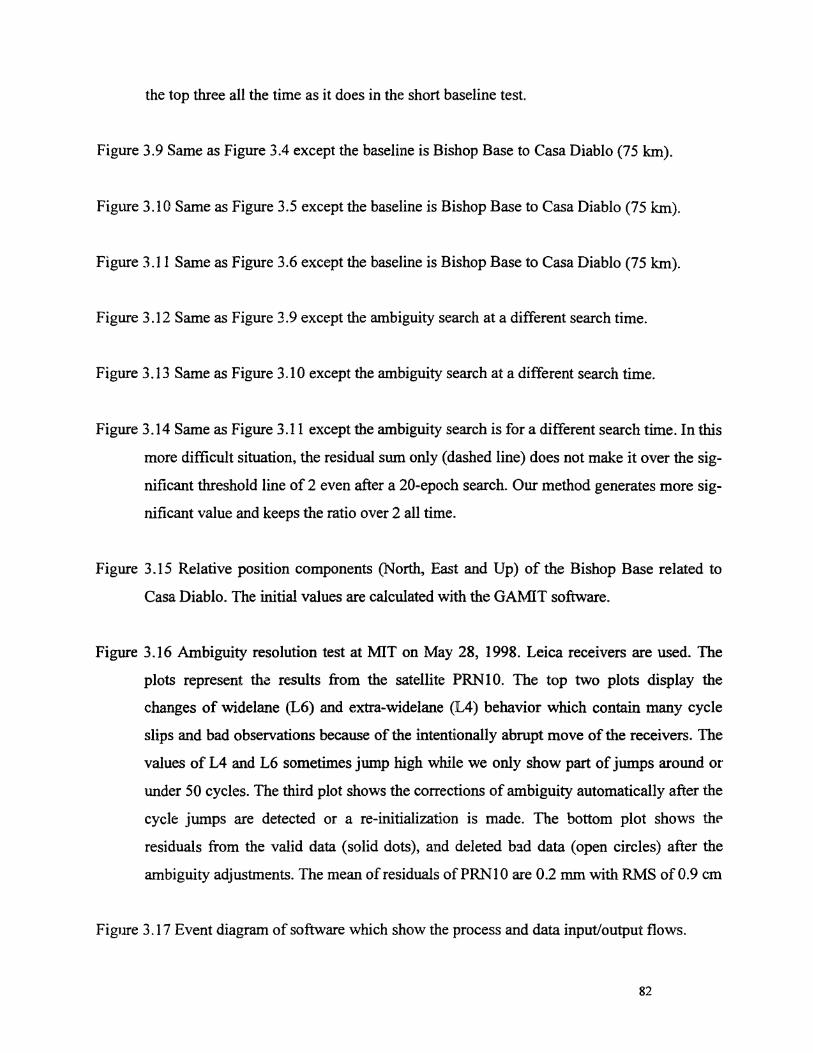
the top three all the time as it does in the short baseline test.

Figure 3.9 Same as Figure 3.4 except the baseline is Bishop Base to Casa Diablo (75 kIn).

Figure 3.10 Same as Figure 3.5 except the baseline is Bishop Base to Casa Diablo (75 kIn).

Figure 3.11 Same as Figure 3.6 except the baseline is Bishop Base to Casa Diablo (75 kIn).

Figure 3.12 Same as Figure 3.9 except the ambiguity search at a different search time.

Figure 3.13 Same as Figure 3.10 except the ambiguity search at a different search time.

Figure 3.14 Same as Figure 3.11 except the ambiguity search is for a different search time. In this

more difficult situation, the residual sum only (dashed line) does not make it over the sig­

nificant threshold line of 2 even after a 20-epoch search. Our method generates more sig­

nificant value and keeps the ratio over 2 all time.

Figure 3.15 Relative position components (North, East and Up) of the Bishop Base related to

Casa Diablo. The initial values are calculated with the GAMIT software.

Figure 3.16 Ambiguity resolution test at MIT on May 28, 1998. Leica receivers are used. The

plots represent the results from the satellite PRNIO. The top two plots display the

changes of widelane (L6) and extra-widelane (L4) behavior which contain many cycle

slips and bad observations because of the intentionally abrupt move of the receivers. The

values of L4 and L6 sometimes jump high while we only show part of jwnps around or

under 50 cycles. The third plot shows the corrections of ambiguity automatically after the

cycle jumps are detected or a re-initialization is made. The bottom plot shows th~

residuals from the valid data (solid dots), and deleted bad data (open circles) after the

ambiguity adjustments. The mean of residuals ofPRNIO are 0.2 rom with RMS of 0.9 em

Figllre 3.1 7 Event diagram of software which show the process and data input/output flows.

82

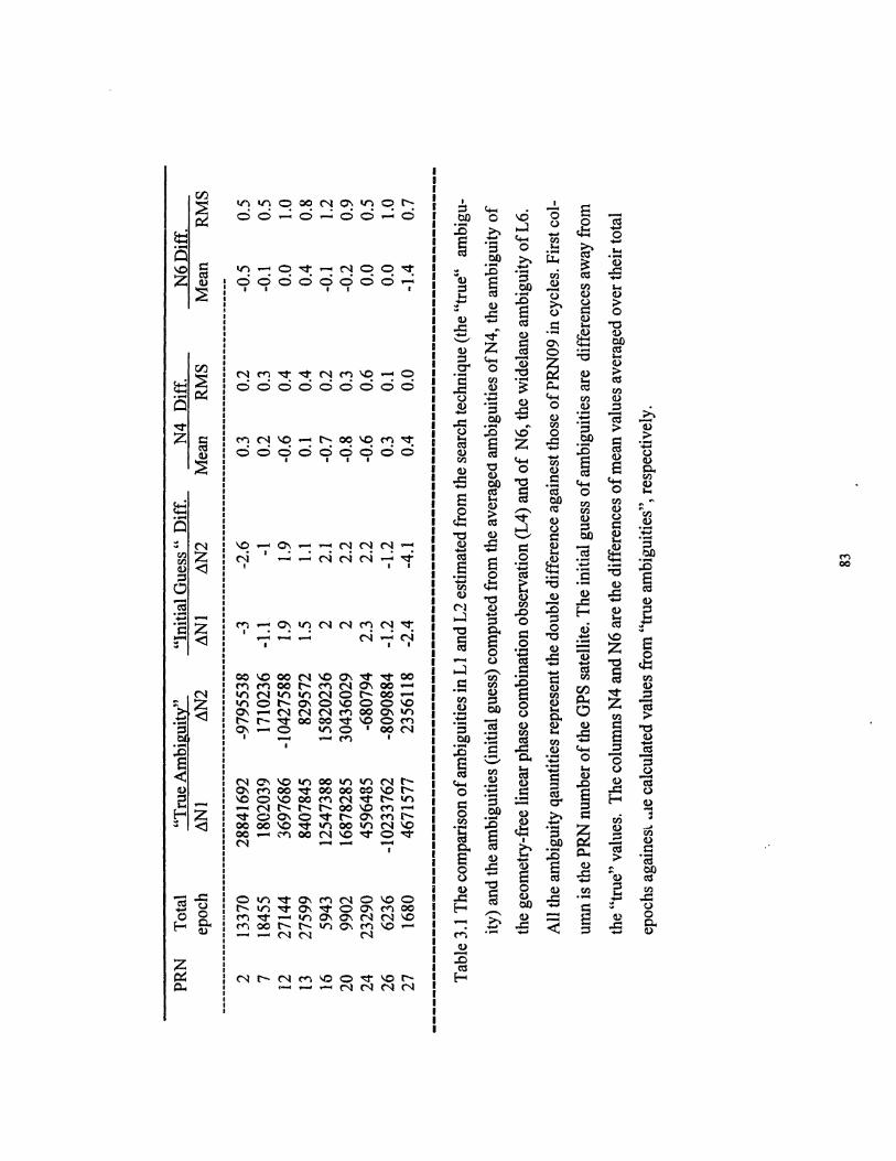
PRN

Tot

al"T

rue

Am

bigu

ity"

"Ini

tial

Gue

ss"

Dif

f.N

4D

iff.

N6D

iff.

epoc

h~Nl

AN

2~Nl

~N2

Mea

nR

MS

Mea

nR

MS

----------------~----------------------~----~~--~--------------------------------~----._---------------------------~----~-----

213

370

2884

1692

-979

5538

-3-2

.60.

30.

2-0

.50.

57

1845

518

0203

917

1023

6-1

.1-1

0.2

0.3

-0.1

0.5

1227

144

3697

686

-104

2758

81.

91.

9-0

.60.

40.

01.

013

2759

984

0784

582

9572

1.5

1.1

0.1

0.4

0.4

0.8

1659

4312

5473

8815

8202

362

2.1

-0.7

0.2

-0.1

1.2

2099

0216

8782

8530

4360

292

2.2

-0.8

0.3

-0.2

0.9

2423

290

4596

485

-680

794

2.3

2.2

-0.6

0.6

0.0

0.5

2662

36-1

0233

762

-809

0884

-1.2

-1.2

0.3

0.1

0.0

1.0

2716

8046

7157

723

5611

8-2

.4-4

.10.

40.

0-1

.40.

7

------------------------------------------------------------------------~---------------------~----

Tab

le3.

1T

heco

mpa

riso

no

fam

bigu

ities

inL

lan

dIJ

2es

timat

edfr

omth

ese

arch

tech

niqu

e(t

he"t

rue"

ambi

gu­

ity)

and

the

ambi

guiti

es(i

nitia

lgue

ss)

com

pute

dfr

omth

eav

erag

edam

bigu

ities

ofN

4,th

eam

bigu

ityo

f

the

geom

etry

-fre

elin

ear

phas

eco

mbi

natio

nob

serv

atio

n(L

4)an

do

fN

6,th

ew

idel

ane

ambi

guity

ofL

6.

All

the

ambi

guity

qaun

titie

sre

pres

entt

hedo

uble

diff

eren

ceag

aine

stth

ose

ofP

RN

09

incy

cles

.Fi

rstc

ol­

Ull

Inis

the

PRN

num

bero

fthe

GPS

sate

llite

.The

initi

algu

ess

ofa

mbi

guiti

esar

edi

ffer

ence

saw

ayfr

om

the

"tru

e"va

lltes

.T

heco

lum

nsN

4an

dN

6ar

eth

edi

ffer

ence

so

fmea

nva

lues

aver

aged

over

thei

rto

tal

epoc

hsag

aine

sl...i

eca

lcul

ated

valu

esfr

om"t

rue

ambi

guiti

es",

resp

ectiv

ely.

83

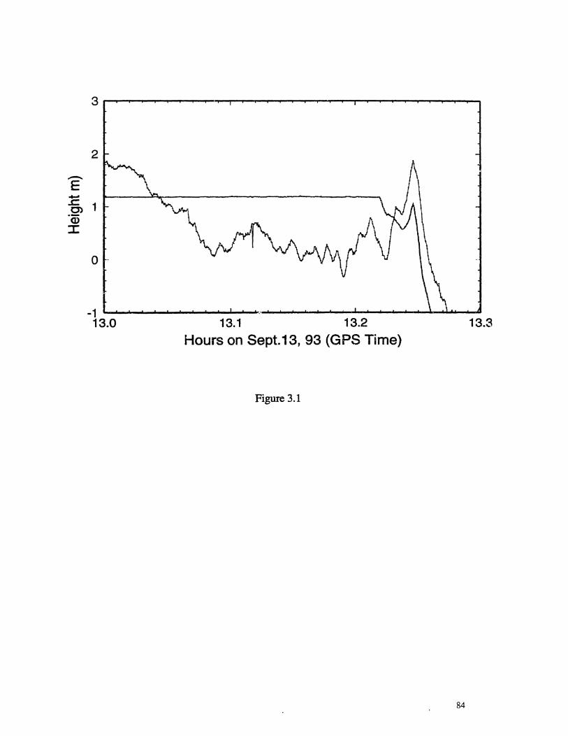
2

13.313.1 13.2

Hours on Sept.13, 93 (GPS Time)

o .

-1 ~I....' ..............'.......__'.......' .....'---.'......,~__--.........................~~....... ~.....a:- ......... -u

13.0

.....-6,1-(])

::I:

Figure 3.1

84

2 PRN13 Widelane L6

en w~J~CD013

>.0

-2

2 PRN07 Widelane L6

enQ)

0(3~(.)

-2

2 PRN13 Extra-Widelane L4

UJQ)

013~0

-2

2 PRN07 Extra-Widelane L4

UJCD13>-0

-2

13.0 13.5 14.0 14.5 15.0 15.5 16.0

Hours on Sept.13, 93 (GPS Time)16.5

Figure 3.2

85

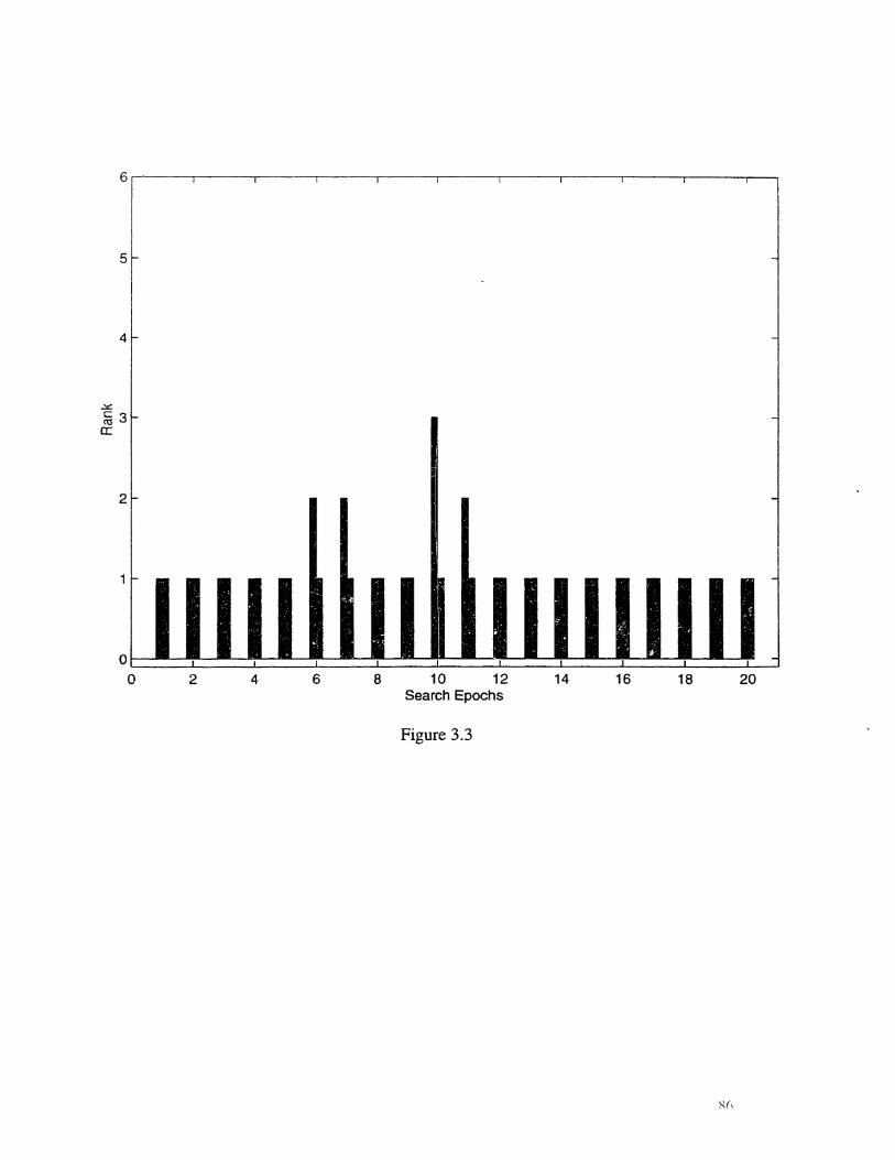
I I I I I I I I I I

~ -

- -

- -

- -

- -

(

- - - "'-- --- i --- I.-- ~ ....... - --- '-- -

6

5

4

2

oo 2 4 6 8 10 12

Search Epochs

Figure 3a3

14 16 18 20

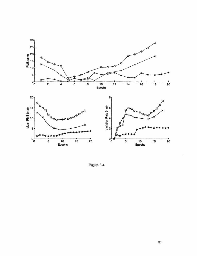
30

25

-20EE;; 15:Ea: 10

5

00 2 4 6 8 10

Epochs

-t'.)1- 14 16 18 20

201510Epochs

5O~--"""""'-_-..Il-__.....I-_-~

o

8

E6S~0::4c:.27ii

~2

201510Epochs

5O~-----'-----'"----~--~o

20

~*lk*****·~.**

.-.15ES-en:E 10a:c:mQ)

:E 5

Figure 3.4

87

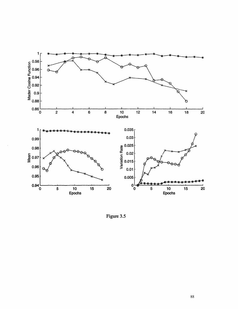
1* * *-~ *--... * * .....

c 0.98.2g 0.96;:,u..Q) 0.94c:-08 0.92~

Q) 0.9"CCd

~ 0.88 \,

0.860 2 4 6 8 10 12 14 16 18 20

Epochs

1~.*****$~**********~

0.035

0.99 0.03

0.98CD 0.025..ata:

c: c:: 0.02m0.97 .Q:E ~ 0.015

L..

0.96 as> 0.01

0.95 0.005

0.94 00 5 10 15 20 0 5 10 15 20

Epochs Epochs

Figure 3.5

88

_-....----

-- .. -.----- . .--.-,.-.-. .. .--.

--- .. --. . .-..-.--.,.\\

\\

"

\\

\-.~.-.-.

\ ' ,,,

\

\

\

\

\

\

\\

\\

\

\\

\\

\\\ -- .....

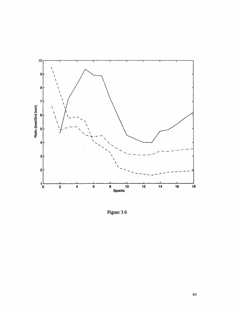
10

9

8

7-enCD.c

'"C 6c£:enCDe 5.Qa;a::

4

3

2....... - ................

1S1614128 10Epochs

6421 ........----.lL-------"-----..-..IO""-"--.......-----......------'-------------'----....o

Figure 3.6

89

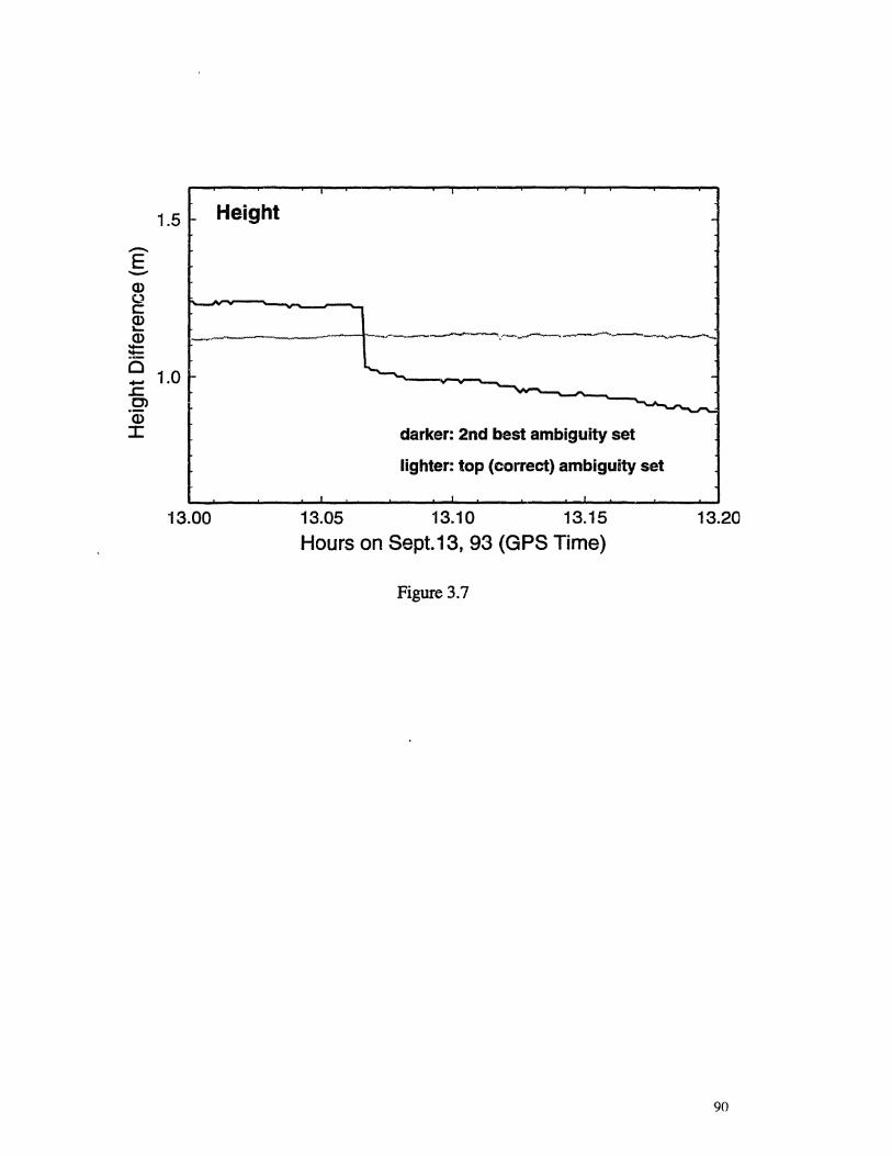
1.5 Height

13.00

darker: 2nd best ambiguity set

lighter: top (correct) ambiguity set

13.05 13.10 13.15

Hours on Sept.13, 93 (GPS Time)

Figure 3.7

13.20

90

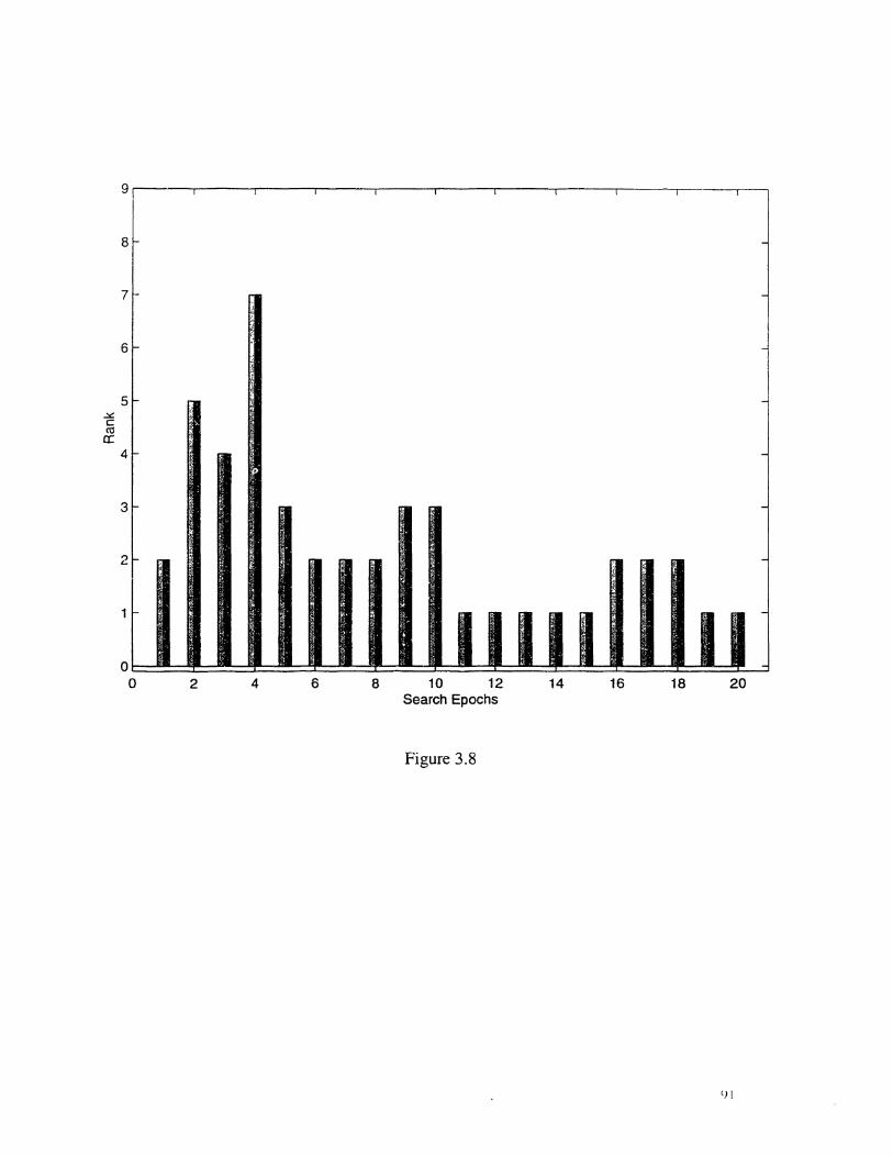
9

8~

7--

6-

5-~

ccoa:::

4-

3~

2-

1 ~

0 - -0 2 4 6 8 10 12

Search Epochs

Figure 3.8

-14 16 18

I

20

() I

-

-

-

-

-

50r

I40~

EE;;; 30~a:

20

10 I

a 2 4 6 8 10 12 14 16 18 20Epochs

45 10

40 E 8....-...E gE'-" 35 CD 6en C5~ a:a: c:~ 30 0 415CD -t::E as

25 > 2

200 5 10 15 ,20 5 10 15 ~O

Epochs Epochs

Figure 3.9

92

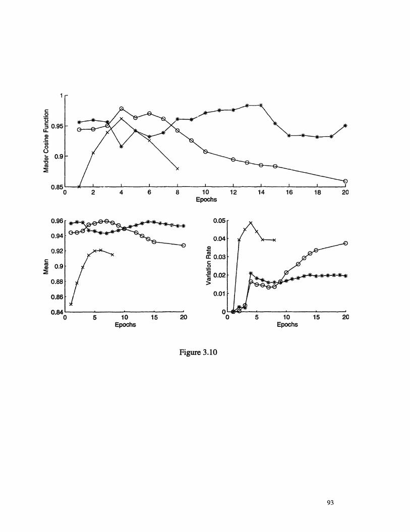
c:.2'0§ 0.95u..Q)c:.Ci)00"- 0.9Q)-0as:E

0.850 2 4 6 8 10 12 14 16 18 20

Epochs

0.96 0.05

0.94 0.04

0.92 CD...asa: 0.03

c: c:as 0.9 .QCD~ 1ii

~ 0.020.88 as

>

0.86 J0.01

0.840 5 10 15 20 5 10 15 20

Epochs Epochs

Figure 3.10

93

2.5 r---~----r------,~--..,...-----,-.----r---,....----r------r----r-----,

2

~~ 1.5-cc:~(J)c»e.Qa; 1a:

.~"~"'-"-.-- .--.--..-

....... --- , ....

0.5

2018161410 12Epochs

8642O"'----....s.---.......---"----......-.-----.---------04----........----&.---~--'o

Figure 3.11

94

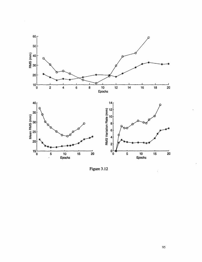
60

50

..-...E 40E

""-"

en:E 30a:

20

100 2 4 6 8 10 12 14 16 18 20

Epochs

40 14

35e12E.......;-10E

E as""-"30 a: 8en c~ .2c: is 6c 25 .t;:CD asCD > 4:2

~en

20 ~a: 2

150 5 10 15 20 5 10 15 20

Epochs Epochs

Figure 3.12

95

.§ 0.95'0c:::s 0.9lLc:

.(ij0~ 0.85Q)-0m~ 0.8

0.750 2 4 6 8 10 12 14 16 18 20

Epochs

0.98 0.07

0.060.96

Q) 0.05...c 0.94 as

~ 0.04('0 0CD ;:

~ 0.92 .~ 0.03

/~~

to

> 0.020.9

0.01* *......

0.88 00 5 10 15 20 0 5 10 15 20

Epochs Epochs

Figure 3.13

96

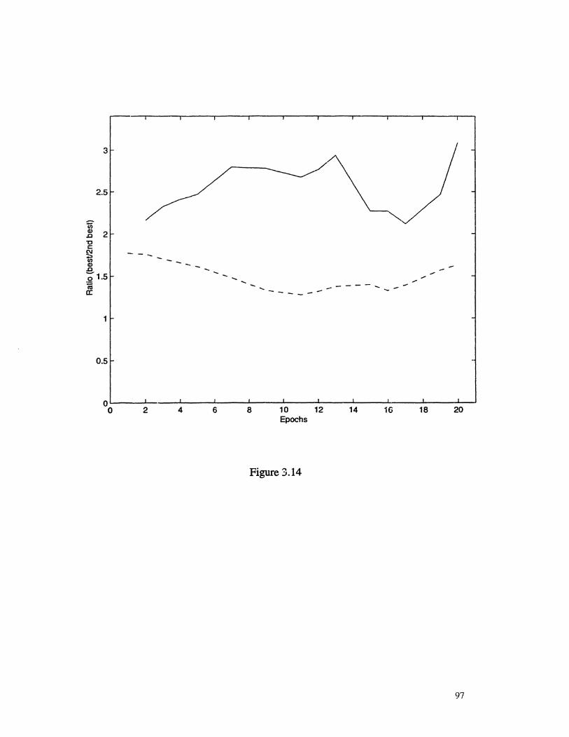
3

2.5

~~ 2-cc:~enQ)..c"';;' 1.5~a:

---......

--- - -- - -

1

0.5

2018161410 12Epochs

8642

o'---__-'-- -'--__......L-__--J..__.--L '--__~__....L.___~____.L_ _I

o

Figure 3.14

97

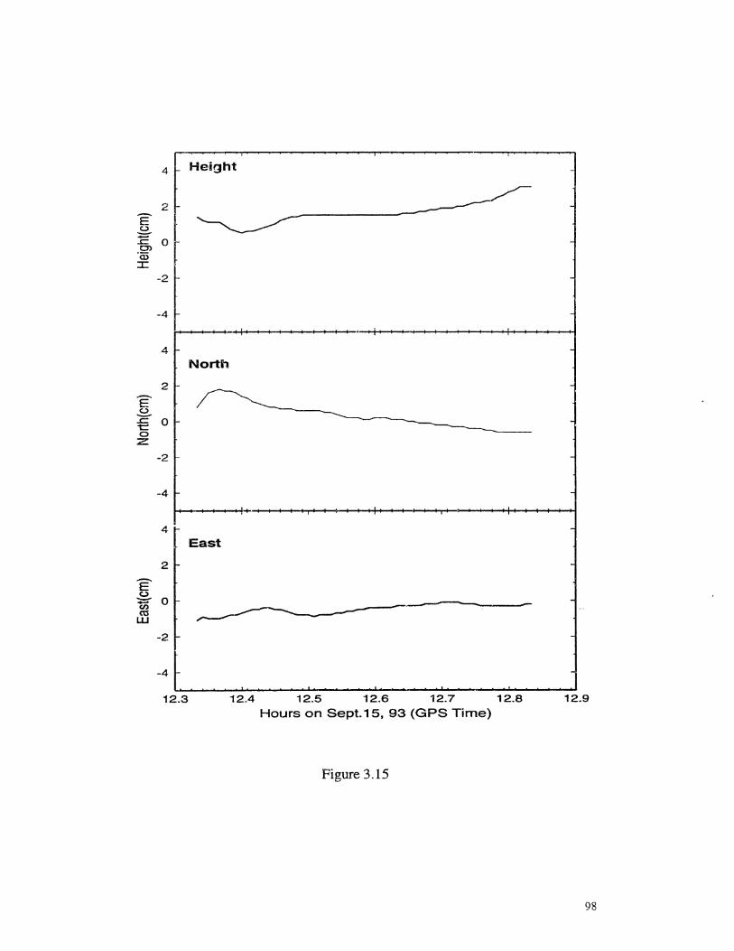
4 Height

2

E~1:: 00)

·03::c

-2

-4

I II I I I I I I I , I ~

4

North

2~

Eu:E' 0 -t::a

Z

-2

-4

I I I I 1-+= I I I I

4East

2.-...E..£. 0en ~

ctSW

-2

-4

12.3 12.4 12.5 12.. 6 12.7 12.8

Hours on Sept.1S, 93 (GPS Time)12.9

Figure 3.15

98

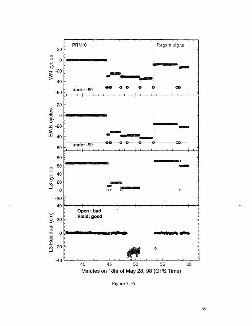
o

-, '

! 7-. .....o

--

---• .n • __UP!

40 45 50 55 60

Minutes on 18hr of May 28, 98 (GPS Time)

Open: badSolid: good

PRf'41 0

------~Gii..--'J!fc:r~G':t-----.cO~~Q_-----oa­

under ...50! ! I

20ena.> 00~()

Z -20?;

-40

-60

20UJCJ.)(3 0~0

Z -20~W -40

-60

80

en 60Q)(3 40>.(.) 20t:t)

....J0

-20

40

..-.-..E 200"-"

(ij:::3

"'C 0-(ijQ)

a:('t) -20..J

-40

Figure 3.16

99

FlowFiles

Start

.....- makcxk.bat

ambiguity.dat

Pre-processor ... SP3 fileRinex NAV file

... PJNEX Obs. fileX file

......new X file (option)

lfuitialize solutionI

loop over .... RINEX Obs. fileepochs X file

PI, P2pas_range.dat....

Ambiguity WL/EWL ambiguity checkSearch cycle slip check

---ml....~ edit info.dat

Residuals_____....~ res info.dat

End

LC

LI, L2,____,...... pOs.....Phase.dat

trajectory filenew X file

model

Output

Summary of Analysis

Loop over

Main Processor

Post-processor

Figure 3.1 7 Event Diagram of software

100

Chapter 4 Kinematic GPS Data Analysis

In order to evaluate the perfonnance of out differential kinematic GPS algorithm and soft­

ware, TRACK, we computed the aircraft tracks with 1993 and 1995 (iPS data collected in Long

Valley surveys. The rrlain aim is to verify the feasibility of GPS in accurate positioning and navi­

gation for aircraft. The geodetic changes of ground uplift rates are not {)ur direct COnCeITl in this

thesis. In this chapter, we focus on the examination of the post-fit phase residuals ofGPS observ­

able calculated from the data analysis. We perform the kinematic tests while the aircraft is static

on the groWld. To further verify the reliability of the software and data analysis when the aircraft

is moving, several overlapping ground tracks of the aircraft, such as these on the taxiway and run­

way, are also displayed and discussed.

4.1 Long Valley Surveys

Selection of flights

The fITst Long Valley survey was p~rfonned in September, 1993 by the SIO team and

NASA T39 crew. Similar surve)'s were repeated between September and October, 1995, and in

November, 1997. One of main purposes of these surveys was to obtain a topographic profile of

the actively uplifting area and its tenlporal changes in the Long Valley Caldera. The other purpose-- ­

was to study the accuracy of the airborne laser measurements for topographic profiling. The

tracks of these flights were designed to be within 100 meters horizontally so that we can make the

cross or overlapping laser footprint paths on the ground for comparison. Each survey contained d.

few experimental days in which the aircraft flew over the caldera twice daily. The horizontal

flight zone covers an area nearly 80 km in the east-west direction and 120 km in the north-south

direction. Some days the aircraft flew a even larger zone. For calibration purposes, several flat

spots on the ground were targeted for repeated overflights: Antelope Springs, Benton Crossing

and Lake Crowley. Antelope Springs and Benton Crossing are both treeless and flat ground sur­

faces within the caldera. Antelope Springs is close to the area \vhere maximmn uplift is expected.

101

Benton Crossing is near the edge of the caldera, somewhat far away from the center of uplift. Out­

side the caldera~ Lake Crowley provides a good flat reflective surface to calibrate the airborne

measurements. Daily height changes of water surface 0n the lake are expected. Direct measure­

ments of lake heights from gauge tide stations on Lake Crowley darn are available and can be

used to remove these daily h.eight changes on the lake so that we can compare the laser measure­

ments of lake heights from different days.

The airborne surveys during these three experiments were carried out by the same aircraft,

NASA T39 jet. The T-39 jet carries a real-tilne pseudorange GPS receiver for high precision on­

board navigation. The flight tracks of the aircraft were pre-designed for repeat flight and the real­

time navigation system enables the aircraft to repeat the flights within 100 meters. The GPS

antennas are mounted on the top of the plane. Two dual frequency P-code GPS receivers (a Trim­

ble 4000 SSE and an Ashtech Z12) were used on board for the 1993 survey [Ridgway et aI.,

1997]. In 1995" only Ashtech Z12 receivers were used. The GPS data collected from these on-

board receivers are used for post-survey processing. Normally, two receivers of the same t)'Pes

are also used on the grounc base station, set on a pennanent land benchmark within a few hundred

meters of the Bishop airstrip where the T-39 jet takes off arld lands. (Figure 4.1).

The laser equipment and GPS receivers placed several requirements upon the geometric

design for the flight tracks. Steep banks of the aircraft will cause the on-board GPS receiver to

lose lock on the signal from the lower elevation angle GPS satellites. The loss of satellite sigl1al

could degrade the trajectory accuracy, introduce cycle slips and, possibly, large time gaps in time

series of GPS data. Therefore, the pilot of the T-39 was advised not to bank more than 10 degrees

and not to make horizontal turns with a radius less than 8.3 kilometers. The tracks are designed as

several segments of short and straight lines over the points of interest connected l)y large radius

turns. The speed of the aircraft is also limited to about 100 meters per second to allow the laser

system to generate a 1 meter radius footprint with 2 meter sarrlpling rate (50 hz laser sampling)

along track. The flight heights of the aircraft are also pre-desigrled for best results in bOtll 1993

and 1995 surveys. The 1993 survey used an ATLAS laser sys~4.em which requires the altitude of

aircraft not to be higher than 1000 meters above the ground to generate the 1 meter radius foot­

print on the ground. Thus in the 1993 survey, the flight heights above topographic ground are nor-

102

mally around 500 meters. The height of aircraft on the flight varied by a few thousand meters

responding to the changes of ground topography in the mountainous area. In tIle 1995 survey, the

T39 aircraft used a new laser system SLICER. SLICER is a medium altitude system which allows

the aircraft to fly higher, at 5000-10,000 meters aoove geoid, so that the flights of the aircraft were

flat even in the mountainous areas of the Long Valley region. In contrast to the pin-point profiling

of the ATLAS system, SLICER generates a 100 meter wide swath comprising sixty I-meter foot­

prints.

The Base Ground Station

The location of the GPS base station at Bishop is shown in Figure 4.1. It is about 500

meters away from the Bishop Airport where the flights began and ended. The antenna is mounted

on a pennanent benchmark. There are two trailers within 30 meters of the antenna.. Due to the

short time of GPS dati recording, we have not assessed the effects of multipath from the trailers.

The position of the base station is calculated both from static (GAMIT) and the kinematic pro­

cessing.. Three GPS stations are used in the static solutions: a Bishop benchmark and two penna­

nent GPS sites at Casa Diablo and Goldstone respectively.. Th~re may be some concerns about the

absolute accuracy of the Bishop position which is based on the Casa Diablo site, which is in the

center of the Long Valley dome, currently uplifting at 20 nun/yr with episodically 40 mm/yr uplift

[Dixon et al., 1997]. In the laser measurement discussed here, only the differential positions

between the aircraft receiver and the base station are needed. Thus the position selection for the

base station does not hurt the calibration accuracy of laser measurement results ..

Data Collection

Our data analysis is based on only the available 1993 and 1995 data which were acquired

by Ashtech receivers, one on the Bishop base station, one on the T-39 aircraft. GPS receivers

record the data at a sampling rate of 2 Hz. The complete GPS data include CIA code pseudorange

and carrier phase, and L2 and L2 P-code pseudorange and their carrier phases frOIT! both ground

and airborne receivers.

103

4.2 Software Use and Data Handling

The analysis package, TRACK, developed in this thesis is documented in software manual

[Chen et al., 1998]. Here we give an overview of the data requirements, program input and output

for the Long Valley Surveying.

Data files

Input data files

TRACK has the abilit)r to deal with both X files (the raw data file in GAMIT) and RlNFX

files. The "Receiver Independent Exchange"~ RlNEX, format is the standard GPS data transfer

fOlTI1at. And was developed for the easy exchange of GPS data from different manufacturers

[Gurtner and Mader, 1990]. Although the data structure of our software is based on the needs of

GAMIT (MIT GPS software), TRACK can read a RINEX data observation file directly. In the

analysis of the data from Long Valley, we used the FJNEX files as inputs. Each file contains

about 25,000 data epochs.

To obtain positions of GPS satellites, the TRACK can either use the broadcast ephemeris

given in the RINEX navigation file, or the more precise ephemerides computed from global data

by a data analysis center of the International GPS Service of Geodynamics (lOS). The precise

ephemeris files can be obtained from one of the IGS archives such as the NASA Crustal Dynam­

ics Data Infolmatioll System center (CDDIS). For the analysis discussed in this thesis, we used

the IGS ephemerides, which had an accuracy '-' 10 ppb in 1993, and --5 ppb in 1995 [Murata et al.,

1995; Goad et al., 1997]. With these accuracies for GPS satellite orbital detennination, the orbital

contribution to the error is less than 1 em in a 100 km baseline. The accuracy of the broadcast eph­

emerides is lower, typically 200 ppb, an error of over 2 em for baselines of 100 km or more.

Output data file

104

Several different data fOffi1ats are adopted for output to meet the needs of users. TRACK

can generate a new X-file with updated position infonnation. This new X-file can be processed by

GAMIT other utilities for further analysis. TRACK can also provide positions as a function of

time in the trajectory file format used in the laser data analysis by other GLAS groups. Other out­

put files include phase residual files and a log file that contains infonnation abollt data edited dur­

ing the analysis. The residual file contains prefit- and J:ostfit- phase residual information for each

satellite at each epoch and is used for data quality checking. The log file summarizes the ambigu­

ity resolutiorl, cycle slip detection, and data editing carried out during the processing. This file can

be used for the post aIlalysis to provide information for data reprocessing.

Ambiguity Resolution

The process model in the Kalman filter allows U~ to predict the positions of the aircraft

epoch by epoch from the velocity obtained from the last epoch. Using the strategy we developed

in the last chapter, we deal with the ambiguity problems in all situations including the ambiguity

initializatioll :md re-initialization during the flights, ambiguity of the new satellite on-the-fly and

cycle slips.

Initial ambiguity

The ambiguity search technique was addressed in Chapter 3. All the searches use fre­

quency constraints to reduce the search number (see details in Chapter 3). In the initial ambiguity

search, the L 1 phase data are typically used for u1.e geometric ambiguity search. Since the starting

position of the T-39 aircraft is within 500 meter of the base station, the ionospheric delay will not

affect the ambiguity search significantly. However, if the search starts with the aircraft a few kilo­

meters of the base GPS station, the ionosphere-free observations, (L3), are used for the geometric

search instead of L 1. The ambiguity searches have been preformed when the aircraft is on the run­

way before and after the flight, and succeed in resolving ambiguities within 20 epochs for 6

flights in 1993 and 1995 surveys by using 2-5 seconds intervaL A larger than recorded interval

(0.5 second) is used to save the search time for a quality ambiguity search. Most of the ambigu­

ities are fixed in the first 10 epochs. The ambiguity search in differellt time periods also shows

105

very consistent results. Due to its position-free character., our ambiguity search technique is also

used to solve the ambiguities during the flights in several cases, and results show that ambiguity

values are as same as those detennined in the static stage of tIle flight.

Ambigui!y for rising satellite

When a new satellite is acquired or a satellite has a cycle slip detected, its phase ambiguity

bias is reset and estimated again. The initial ambiguity search strategy can work in this case. To

save processing time, however, wIlen a single cycle slip occurs or a new tiatellite rises, most of the

time, we use a faster way (see more details in Cha?ter 3 to detect and fix the cycle slips and esti­

mate the initial bias for new satellit\?s directly. In dual frequency applications, utilizing the iono­

spheric delay estimates fronl other satellites, the ionospheric effect in the ray direction of this new

satellite is estimated to reduce its impact in the ambiguity resolution.

!dcle slip~ and data editing

In the TRACK software, we use the ionospheric reduced geometric observations L6 and

L4, a method discussed in Chapter 3, to detect possible cycle slips before processing phase data.

This action is made in a pre-processing editor we designed (See the diagram in Figure 3.17).

Most cycle slips can be detected by the widelane and extrawidelane check.Due to the

nature of the linear combination LI-L2 in the widelane observations, however, there are rare but

possible cases undetectable by this method that the same jumps occur in L1 and L2 at the same

time. Residual check is the nonnal tool for cycle slip detection. In the kinematic survey, tile pre­

fit residuals DiLl and L2 are of little use because of the movement of the receiver. The only hope

to use the residuals is after estimating the positions of the receiver. The unmodeled errors remain­

ing in residuals, such as multipath, unmodeled atmospheric effects, vary smoothly over a short

observation time. These result ill residual changes which vary smoothly from epoch to epocll in

the absence of cycle slips. Our post-data editor relies on this behavior to detect the possible

remaining cycle slips by checking the residuals and residual changes for each satellite.

106

Another technical problem for data checking is the similar nature of a single outlier and a

cycle slip in the residuals. It is impossible to distinguish an outlier from a cycle slip instanta­

neously. Therefore, we develop (l strategy to utilize the variation of residuals over a small time

period (10 epochs) to identify whether the jump is isolated (outlier) or a pennanent shift (cycle

slip).

First the residuals in each observation at tl1e currellt epoch are checked and sorted from

maximum to minimum. If a large value occurs for one satellite data residual, a suspect is found. If

this occurs when a new satellite comes at this epoch, we assume that the problem is in its uncor­

rected initial ambiguity guess. Otherwise, we continue to check the suspects one by one from tlle

largest to the smallest. An abnormal jump in one satellite observation may transfer its erratic

change into other observations. We begin with the one that has the maximum jump. The average

values of residuals of this suspect over 5 epochs on both sides of the jump are calculated sepa­

rately with their RMS scatters. If the suspect's residual value is far away from both averaged val­

ues, an isolated bad datum is found and marked. If the averaged values on both sides are not close

and separated by more than three sigma of their RMS scatters, a cycle slip is possible. The next

action is to find whether it is on Ll or L2. N"rmally, both Ll residual and \¥idelane ambiguity

(WL) are used to determine such situation.

Phase center correction

The rim of the antenna in Bishop base station is measured for each experiment. The con­

stant height differences for both L 1 and L2 phase centers frc m the rim are obtained from the man­

ufacturer's manual for the same type. The antenna mounted on the roof of the T-39 aircraft is very

special, and we don't have any infonnation on it. The offset correction for the GPS receiver to the

laser spot was measured for the T-39 aircraft when the aircraft was the ground. Thus the phase

center offset is absorbed into this correction of the calibration.

107

4.3 Kinematic GPS Data Processing and Analysis

Our GPS kinematic processing begins by using pseudoranges PI or P2 to obtain an

approximate (precision of 1-2 meters) trajectory for the flight. An example of the static portion of

a flight is shown in Figure 4.2. The goal of this solution is to check the quality of the data series. It

also provides the mean values of widelane ambiguities (L6) and extra wide lane ambiguities (L5)

and their associated RMS scatters for the cycle slip detection. Furth~nnore, if there are no cycle

slips during the processing, these average values over the entire observation time span can also

provide a quality estimation of the scale size for the ambiguity search space.

Next we perform the initial ambiguity search which is necessary for carrier phase data

processing. lnere are five parameters controlling the search: the number of primary satellites, the

allowance of noise level ill the L l/L2 ambiguity integer relationship, the search range for each

ambiguity, the epochs used for accumulating RMS, and the observation type for the geometric

search. Generally when the aircraft is on the runway, we use a 0.1 or 0.12 cycle as the dual fre­

quency lane constraint for these short baselines. Several larger or smaller constraint values (0.3 ­

O~08 cycle) are also tested but there is not much difference in tile results except the search time.

We still obtain the correct ambiguities in tllese cases. The 0.1 or 0.12 dual frequency lane con­

straint is detennined empirically by several tests in our experiments. For the number of the pri­

mary satellites, we nonnally include all satellites over 15 degree elevation angle at frrst, then

adjust it according to the behavior of satellite with low elevations. Sometimes a cutoff of 20

degrees is applied to avoid the multipath in lower elevation angle observ~tions. Following the

examination of the behavior of its widelane and extrawidelane integers, we extelld the search

range by ten or fifteen integer on each side of the initial ambiguity guess for each satellite, which

means that each satellite could have 21 or 31 candidates in the search space dimension. When the

baseline from the aircraft to the GPS base station is short, the ionospheric effects do not play a

significant role on the solution. L 1 is used for the geometric analysis for the search instead of the

iOIlosphere-free combination L3. For most experiments, when a data sampling rate of 5 or 10 sec­

onds is used, a ten-epoch time duration of continuous search is enough for fixing and validating a

significant ambiguity set. The initial ambiguity search is nonnally performed in j}e static on-run­

way position of flights, but this does not mean this searcll technique only works for the static situ-

108

ation. The ambiguity search technique we have implemented is position-free. l~ests of the

algorith.-..rn are applied when the aircraft was running on the runway and when it is flying in the air.

These tests results yield the same ambiguities as those from the static determination if there are

cycle slips occur during the time gaps of the different testing epochs.

After the initial ambiguity set settles down, phase observations of L1 or L3 are used for

precise trajectory determination. In this stage, loose constraints are used normally 1 meter for data

noise and <Pw of 9x104 m2/s for the aircraft position process noises in three directions, together

sufficient to cover the maximum aircraft velocity changes (Wlder 300 mls) in any situations dur­

ing surveying. After analyzing the residual behavior of the data and performing some editing, we

use strict constraint for the data noise (0.5 - 5 em) and cI>w of 102-104 m2/s for position process

noise to take the advantage of the more accurate prediction of the aircraft velocity.

Trajectories of T-39 for the 1993 experiment

Three flight surveys were perfonned from September 13 to 15,1993. We display theirtra­

jectories in Figure 4.3 to Figure 4.5. In the 1993 survey, the aircraft flew at 2000 to 3000 meter

above the ellipsoid to keep the aircraft 500 meter above the ground. Only the Ashtech receivers

were used for the aircraft solution. L3 phase observations are used to eliminate the ionospheric

effects on GPS measuremeIlts. The base station receiver had several problems during the middle

of the flight on Sept. 14, apd only two-thirds of the data could be used (Figure 4.4). The total

flights in the 1993 survey can be divided into 18 straight line sections for laser data measure­

ments. The Jrajectories are almost identical day to day to repeat ground tracks but with altitudes

that may differ by a few hundred meters. In our precise kinematic mode, the precision of the posi­

tions during flights for a single epoch estimate is 2 - 4 centimeters horizontally, and around 3 - 9

em vertically when a 5 em L3 phase noise is used. When a 5 nun measurement noise is used, the

precisions of the positions are 0.4-0.6 em horizontally and 0.9-1.2 em vertically. The sigma

changes during the same flights are due mainly to the changes of satellite constellation (Figure

4.6).

109

In Figures 4.7 to 4.9, \ve 11lH~trate the residual behavior during the 1993 airborne tests.

The residuals from all satellites show variations under 0.1 cycles (nearly 2 cm for L3) after data

cleaning, ambiguity and cycle slip fixing. In some time scans, the flat behaviors of residuals are

due to the low availability of GPS satellites (down to 4). Also the same satellites show similar

behaviors of residuals for the three surveying indicating systematic errors. These errors may come

from the multipath from the aircraft wing because the aircraft flew the same flight tracks mostly at

the same time for each day ..

The adding of zenith deluY estimates does not change the solution significantly. The alti­

tude position differences are mostly under 1 cm although sometimes tlley are over 1.. 5 em between

cases Vlith and without zenith delay estimates.. One possible reason for the good aspect is that the

tests were conducted under good weather with a calm atmosphere. The possible variations of

atmospheric zenith delay are small and are negligible for the slight elevation angle difference of

the same satellite signal obtained by two GPS receivers .. We tested different atmospheric mapping

functions with MTT [Herring, 1991], NMF [Niell, 1996] and CfA [Davis, 1986] models .. The

results among ~iifferentmapping functions are very close .. It suggests that at low altitude (less than

2 km above the ellipsoid) and for the observations above 15° elevation angles, there are no impor­

tant differences among the current atmospheric mapping functions .. The qualiry of estimation of

au--nospheric effect is h.urt by the low satellite availability .. In several time spans, the number of

common observable satellites drops to only 4 (Figure 4 ..6), in v~hich case we can't estimate all the

parameters uniquely .. In these cases, estimates are possible because the process noise constrains

the atmospheric delay parameter estimate ..

The phase residuals for the three days are similar (Figure 4.7 - 4.9) maybe because the

schedule of flight are almost the same Vlith the same flight time and route .. The similar and non­

white-naise-like behaviors of residuals indicates that the remaining errors may come from the

multipathing which results from the similar ground environment \vhen the aircr8.J.+t is on the

ground aila from the wing of the aircraft especially when the aircraft banks in a designed flight

route.

110

Trajectories ofT-39 for the 1995 experiment

Similar flight surveys were performed from September 28 to October 10, 1995. Figures

4.10 - 4.12 show the trajectories of the Sept. 28, 29 and 30 flights. The results show behavior sim­

ilar to those in the 1993 surveys. The altitudes of the aircraft in the 1995 surveys are higher

(around 5 to 10 Ian above the ellipsoid) designed for middle range altitude measurements with the

new laser instrument SLICER [Hofton et aI., 1997]. Also, the horizontal range of flights is much

broader. The residuals from the solutior! of these two experiments are shown in Figures 4.13 to

4.14. On some days such as Sept. 28, the RMS scatters are little higher than those in 1993 surveys.

We tested with higher elevation cutoff angle of 17° and 20° and the aVt;rage residuals reduced 5%

and 7% respectively.

4.4 Calibration Analysis on the Airport

4.4.1 Airport Static Tests

The validation of the accuracy ofkinematic GPS surveying is not easy to perform because

it is hard to require the aircraft to reoccupy the same spot exactly before and after the same flight

and between the flights. One way to test the software is to use the data from the static stage of the

aircraft positioning. Figure 4.15 shows the ,position of the aircraft on the ground before the Sept.

13, 1993 flight. The estimated heights are very flat and stable even wilen satellites rise or set dur­

ing the interval. The RMS scatters of the positions then means about 2-3 em, north, 2-3 em, east

and 3.3 em, height assuming a 5 em L3 phase data noise.

In Figure 4.16, we show the autocorrelation functions of the height variations when the

aircraft sat on the runway. The autocorrelation functions from different surveys indicate the mea­

surements errors in our GPS kinematic surveys are dominated by the high frequency errors in the

GPS signals. The autocorrelation length is defmed as the lag for which -:he normalized autocorre­

lation function to lie. In our surve)'s, the auto-correlation lengths are 73.0, 136.5, 66.5 seconds for

II I

the experiments on Sept. 13-15, 1993~ and 48.0,77.0 secon\1s for those OIl Sept. 28 and 30,1995,

respectively. Thus data noises of the GPS signals can be averaged out in less than 80 seconds for

most days; an exception is Sept 14, 1993 for whicll auto-cOITelation length is over 2 minutes.

To test the capability of our software and algorit.hm ill ambiguity fixing and data analysis,

we processed the data independently in the kinematic mode cmd the quasi-static mode., In Figure

4.17, we display the positions of the aircraft on the runway at the end of the flight on Sept. 13,

1993. For the kinematic survey mode, we used a loose constraint (4x104 m2/s ofCl>w) for positions

which can cover the movements of the aircraft under a velocity of 200 mls even it is still at the

static stage. The ambiguities are calculated by the search techrtique when the satellite comes into

the analysis durinf~ the flight. In the "quasi-static" processing, we started the ambiguity search

calculation with the data after the aircraft fInished the flight, but used a 0.01 mls velocity con­

straint for the "quasi-static" process noise. The darker line in Figure 4. I7 represents the kinematic

results, and the lighter line represents the static mode survey results. The t\vo "trajectories" agree

with each other within 1 em for most of the common observation period; the average difference is

just 4 mrn. This test indicates that the solutions from our software is unique and independent on

the starting times as long as the ambiguities are fixed appropriately and the process noise used can

cover the motions ofaircraft.

4.4.2 Runway Kinematic Tests

To further test our kinematic analysis in the moving portion of the surveys, we processed

several spans of data acquired when the aircraft moved on the runway at low and higll speeds.

There is only one runway and one taxiway at the Bishop airport. All the aircraft take off and land

on the same !1Ltlway, so that the measured heights of the aircraft on the runway and taxiway pro­

vide us with a qualified calibration location to compare the aircraft tracks calculated from differ­

ent days. Although there may be height variations when the aircraft runs through different paths

within a few tens ofrrleters in the width of the runway and taxiway, the runway and taxiway are

still relatively flat. The altitude of aircraft on the runway becomes a valuable means to assess the

kinematic data quality. In this section, we compare the aircraft trajectories obtained in two exper­

iment years (1993 and 1995).

112

In Figures 4.18-4.21, W~ show the tracks of aircraft running on the taxiway before take-off

and after landing as well as its take-off and landing portion on the main runway. The tracks are

calculated from the six flights during 1993 and 1995 surveys. The runway and taxiway lie mainly

in north\vestem to southeastern direction and are 10DO-plus meters long (Figure 4.18). The taxi­

way links the main runway to the airport. In the data analysis, the ground heights show ,,"ariations

around 5 meters in runway and taxiway (Figure 4.19).

We display the detailed GPS estimated height variation on the taxiway in Figure 4.20.

\l/hen the T-39 runs on the taxiway, the aircraft's speed is slow and well under 10 mls. The maxi­

mum of differences between all reported tracks is under 8 centimeters on the taxiway. We used

the differential height to eliminate the height slope changes in the horizontal direction. All tracks

are recalculated relative to the track measured on Oct. 5, 1995. and results are shown in the lower

plot of Figure 4.20. The analysis shows an average difference of 1.7 em. The internal RMS scat­

ters of each track are averaged to only 0.9 cm suggesting some systematic biases may exist. Sev­

eral factors could contribute to the systematic differences, including mechanical reasons such as

different tire pressures, and the ground height variations in the different running paths in the taxi­

way.

In Figure 4.21, we shows the detailed GPS estinlated height variations when the aircraft is

on the main runway during take-off. In these situations, the aircraft's speed averages 30 - 50 mls

and could be up to 60 - 70 mls. The results demonstrate high consistency in cases ofboth high and

low speeds. The differences oftraclcs measured in the six flights during 1993 and 1995 tests show

that when the aircraft runs on the ground, the estimated heights of the GPS antenna are consistent

within 4 em, and under the uncertainties for single epoch measurements. The T-39 aircraft lands

and takes off at different points on the runway in different experiments. We plotted the take-off

and landing tracks in -Figure 4.22 for experiments conducted on Sept. 13 and 15, 1993~ and on

Sept. 28 and 30, 1995. As soon as the aircraft is running on the ground in both cases, the estimated

heights of the GPS antenna are consistent within 6 em for most parts of tracks. The mean differ­

ences are 1.8,3.1,2.5 and 1.2 em for experiments conducted on Sept. 13 and 15, 1993, and on

Sept. 28 and 30, 1995, respectively. Figure 4.23 shows more details of the runway track for take-

113

off and landing tracks on Sept. 30, 1995. The measured landing height of the aircraft on the run­

way repeats almost exactly the takeoff track after nearly a 4 hour 11i~ht. The good agreement

between the runway positions before the take-off and cfter the landing in t1l~ same flight demon­

strates the reliability of ambiguity resolution in our algorithm. If we mishandle the cycle slip and

initial ambiguity bias for any satellites during flight, we would have obtained an end position far

away from the initial position. The high consistency between the different flights shows that GPS

has the ability to obtain a em-level precision position for aircraft tracking at high speeds. Even

after two years, most of the flights fit into old tracks within a few centimeters in their height mea­

surements.

114

References

Chen, G., T. A. Herring and R. W. King, TRACK software manual, MIT, in preparing, 1998.

Goad, C.C., Grejner-Brzezinska, D.A. and Yang M., Determination of high-precision GPS orbits

using triple differencing technique. J ofGeodes)J; 70, p. 655-62, 1997

Gurtner, W., G. Mader, The RINEX Format: Current Status, Future Developments. Proceedings

oJ"the Second International Symposium ofPrecise Positioning witll the Global Positioning

system, Ottawa, pp977, 1990.

Hofton, M., J. Blair, B. Minster, J. Ridgway, D. Rabine, J. Bufton, and N. Williams, Using laser

altimetry to detect topographic change at long Valley caldera, California, Earth Surface

Remote Sensing, SPIE 3222,295-306, 1997.

King, R .. & Bock Y., Documentation for the GAMIT GPS ..t\nalysis Software, MIT GeodeS)) and

Geodynamics Lab, 1998.

Martin C., GITAR program documentation, NASA contract number NAS5-31558, GOtldard

Space Flight Center, Wallops Flight Facility, Wallops Island, VA, 1991.

Murata, M.; Harigae, M. and Tsujii, T., GPS positioning with broadcast and precise ephemerides,

SICE '95. Proceedings ofthe 34th SICE Annual Conference, p. 519,1995

Remondi, B. W., NGS Second Generation ASCII and Binary Orbit Formats and Associated Inter­

polation Studies, Poster session presentation at the Twentieth General Assembly of the

IUGG, Vienna, Austria, August 11 - 24, 1991.

RidgwaY,J.R.. , J.B. Minster, N.P. Williams, J.Lu Bufton, and W .. Krabill, Airborne laser altimetry

survey of Long Valley, California, Geophys. J./n.t. 131,267-280,1997.

115

Figure Captions

Figure 4.1 Locations of the airport and the base GPS station at Bishop, California. The circle is

the geodetic position of the GPS receiver mounte(i on a pennanent benchmark as the refer­

ence station. There are two trailers (lighter rectangles) near the GPS ground recej·ver. At

500 meters southeast is Bishop Airport, where; the T-39 aircraft, parked on the runway

during experiments in 1993 and 1995. The diamond dark spots represent several different

starting positions of flights for the aircraft.

Figure 4.2. Relative height values for the aircraft while it was stationary calculated~ from PI (the

darker line) and P2 (the lighter line) single frequency code measurements during the Long

Valley survey on the Sept. 28, 1995. The difference in the average height is 14.7 em over

30 minutes. Because the distance between the GPS base receiver and the GPS aircraft

receiver of the base station is short « 1 km), unmodeled atmospheric and ionospheric

effects are not likely to contribute to these differences between PI and P2 solutions. Range

data noise and the multipath contribute mostly to the differences.

Figure 4.3. The trajectory of the aircraft during the Long Valley survey on Sept. 13, 1993. We

used the WGS-84 ellipsoidal system as the reference s)"~i.c!l1. The heights are L~e ellipsoi­

dal elevations (upper plot) and vary to keep a 500 meter relative height over the ground for

ATLAS laser measurements. This flight repeats the measurement sections (straight lines

in horizontal trajectory) over crossover points (Antelope Springs and Benton Crossing)

and along lake Crowley twice.

Figure 4.4. The trajectory of the aircraft in the survey on Sept. 14, 1993. The trajectory is not

completed due to the receiver problem on the ground base station. (see Figure 4.3 for

detailn)

Figure 4.5. The trajectory of the aircraft in the survey on Sept. 15, 1993. (see Figure 4.3 for

116

details).

Figure 4.6. "The top plot shows the uncertainty values of the estimated heights of the aircraft cal­

culated with (the darker line) and without (lighter line) atmospheric (ATM) parameters

(the lighter line). Data analyses are perfonned with the L3 data of Sept. 13, 1993. In the

bottom plot, we show the satellite availability during the entire flight. The elevation cutoff

angle for observations is 15 degree. At times, the total PRN satellite number is just four,

which makes the solution with atmospheric variations a little worse. When the satellite

availability is down to 5 or even 4, the uncertainties ofposition determination can up to 20

cm for the height. When the data noise is assumed to be 5 em, The smoothness in the

changes of the height uncertainties when the atmospheric parameters are estimated and the

number of satellite changes is due to the process noise on the ATM parameter.

Figure 4.7, Post-fit L3 phase residuals for some satellites from Sept. 13, 1993 data analysis. After

the fixing of cycle slips, there are no over 0.2 cycle (3.8 em) for any of the observations.

l·he ambiguities for new satellites that rose during the flight appear to be resolved cor­

rectly, so that there are no jumps in the residual time series when satellites come in or drop

out of the solution. The RMS scatters of the residuals in each frame are 0.8, 0.9, 1.2, 1.1,

1.1,0.6,0.8,0.9 em for satellites PRN16, 02, 07, 09,12, 13, 24, and 26, respectively.

Figure 4.8, Residual variations of some satellite observations used in the calculation for the air­

craft GPS data analysis on Sept. 14, 1993. (See similar comments in Figure 4.7)

Figure 4.9, Residual variations of some satellite observations used in the calculation for the air­

craft GPS data analysis on Sept. 15, 1993. (See similar comments in FiglIre 4.7)

Figure 4.10, The trajectory of the aircraft on Sept. 28, 1995 calculated by our kinematic GPS soft­

ware. The elevation of aircraft flight is over 5 kIn for middle altitude laser survey using

SLICER. At such height, the aircraft could fly horizontally without worrying about the

mountains. The horizontal region is also extended compared to the 1993 surveys (Figures

4.4-4.6).

117

Figure 4.11, The trajectory of the aircraft on Sept. 29, 1995 calculated by our kinematic GPS soft­

ware.

Figure 4.12, The trajectory of the aircraft on Sept. 30, 1995 calculated by our kinematic GPS soft­

ware. The elevation of aircraft flight is at the level 5 km and 10 km. The horizontal region

also extends to be almost ac; twice large as that in the 1993 surveys.

Figure 4.13, Residual variations of some satellite observations used in the calculation for the air­

craft GPS data analysis on Sept. 28, 1995.

Figure 4.14, Residual variations of some satellite observations used in the calculation for the air­

craft GPS data analysis on Sept. 29, 1995. As the relative height and horizontal distance

increase for two GPS receivers, the differential GPS cannot efficiently eliminate all eleva­

tion-related model erlors, so the residuals show more noise than those for the lower height

flights of the 1993 surveys.

Figure 4.15 a) The tracks (Up, North, East) for the T39 aircraft sitting on the runway before takh,g

off on Sept. 13, 1993. The results are derived from differential GPS tracking with two

ASHTECH GPS receivers, one on the base station, the other on the roof of the T39 air­

craft. L3 is used for the calculation.

b) The track changes for the T39 aircraft sitting on the runway before taking offon Sept. 14,

1993.

c) The track changes for the T39 aircraft sitting on the runway before taking offon Sept. 15,

1993. The variations are larger than those from Sept. 13 and 14 possibly be caused of the

strong multipath from the aircraft parking place on this date.

Figure 4.16. The normalized autocorrelation functions of the time series of estimated height errors

of the aircraft. The data are from surveys on Sept. 13-15, 1993, Sept. 28 and 30, 1995

when the aircraft sat on the runway. Data sampling is 2 Hz. The flat line is the lie value

which defines the autocorrelation length. The lighter line (the most outside line) is from

118

the Sept. 14,1993 survey.

Figure 4.17. The trajectory of the T39 aircraft sitting on the runway after landing (Sept. 13,1993).

In the upper plot, the darker line represents the results continuing from the kinematic cal­

culation which started before the aircraft took off. Then we start an independent static sur­

vey after the T39 aircraft landed (the lighter line). The position process noise of <Pw is

chosen as 10-4 m2/s for the "static" mode comparing to the 104 m2/s used in the kinematic

lnode. The two lines agree well in their height variations. The lower plot shows their dif­

ferellces which is averaged less than 1 em.

Figure 4.18. Aircraft tracks estimated from our GPS kinematic analyses both in the 1993 and

1995 surveys. The tracks are results from Sept. 13-15, 1993; Sept. 28, 30 and Oct. 5, 1995.

Plot shows tracks of the aircraft running on the runway (horizonta} view)

Figure 4.19. Aircraft tracks estimated from our GPS kinematic analyses both in 93's and 95's sur­

veys. The tracks are results from Sept. 13-15,1993; Sept. 28,30 and Oct. 5,1995. Plot

shows altitudes of the aircraft running on the runway in the east direction (vertical view)

Figure 4.20. Detailed estimated track heights of the aircraft on the taxiway with the GPS kine­

matic surveying. The upper plot is enlarged from Figure 4.19 with the same data. This plot

shows the aircraft running on the taxiway with speed less than 10m/s. The lower plots

shows how the other five tracks differ from the track ofthe Oct. 5, 1995. The averaged dif­

ference is 1.7 em for five track differellces. The averaged internal RMS for each track is

0.9 em..

Figure 4.21. Detailed. estimated track heights of the ~:~craft on the main runway during the take­

offs. The upper plot is enlarged from Figure 4.19 with the same data. The data come from

days 8ept. 13, 14,15 of 1993 and Sept. 28,30 and Oct. 5 of95. This plot shows the aircraft

running on the runway with low to high speed 10 - 70 mls. The lower plots shows how the

other five tracks differ from the track of Oct. 5, 1995. The error bars are 4.1 em, the single

epoch vertical uncertainty in the track obtained on Sept. 30, 1993.

119

Figure 4.22. Comparison of the estimated track heights of the aircraft on the main runway when

aircraft is taking off and landing with high speed (40-70 m/s). The data are obtained from

days Sept. 13, 15 of 1993 and Sept. 28, 30 of 1995. The darker line is the landing track

while the lighter line is the tqkeoff track.

Figure 4.23 Enlarged portion of track heights of the aircraft on the main runway during takeoff

and landing for experiment on Sept. 30, 1995.

120

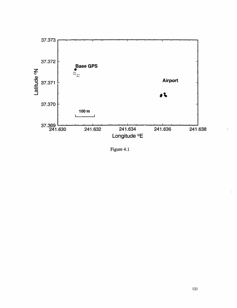
37.372Base GPS

Z •0 Lt r~CD ~~

-0 37.371 AirportT-.....~C\1..J ,\

37.370

100m

37.369241.630 241.632 241.634 241.636 241.638

Longitude °E

Figure 4.1

121

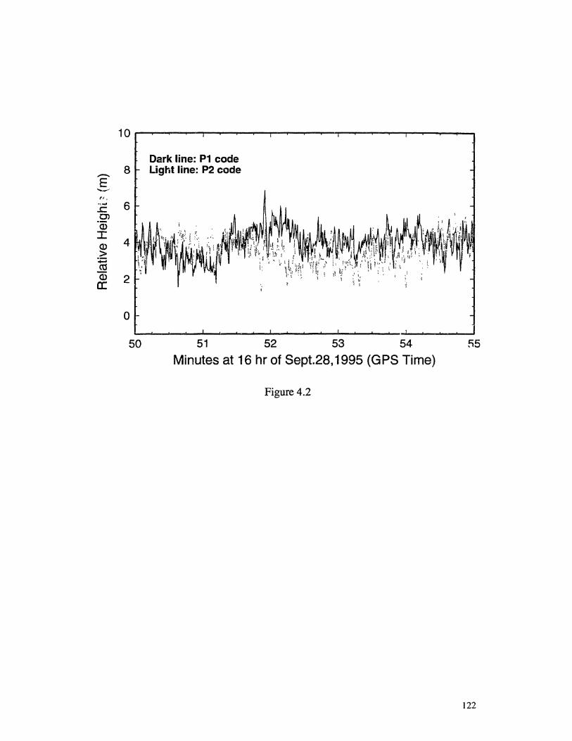
f/,

8Dark line: P1 codelight line: P2 code

o

50 51 52 53 54

Minutes at 16 hr of Sept.28,1995 (GPS Time)

Figure 4.2

tiS

122

4

2

1 ~~ ~ ~

13.0 13.5 14.0 14~5 15.0 15.5 16.0 16.5

Hours on Sept.13,1993 (GPS Time)

Circles:Antelope SpringsBenton CrossingLake Crowley

120km38.2

37.2 -

38.0

37.8Z0

CD-c::::J~

37.6:;=m

....J

37.4 Bishop

37.0 ............~......................~..........~........................................,...........~...................................,240.8241.0241.2241.4241.6241.8

Longitude °E

Figure 4.3

123

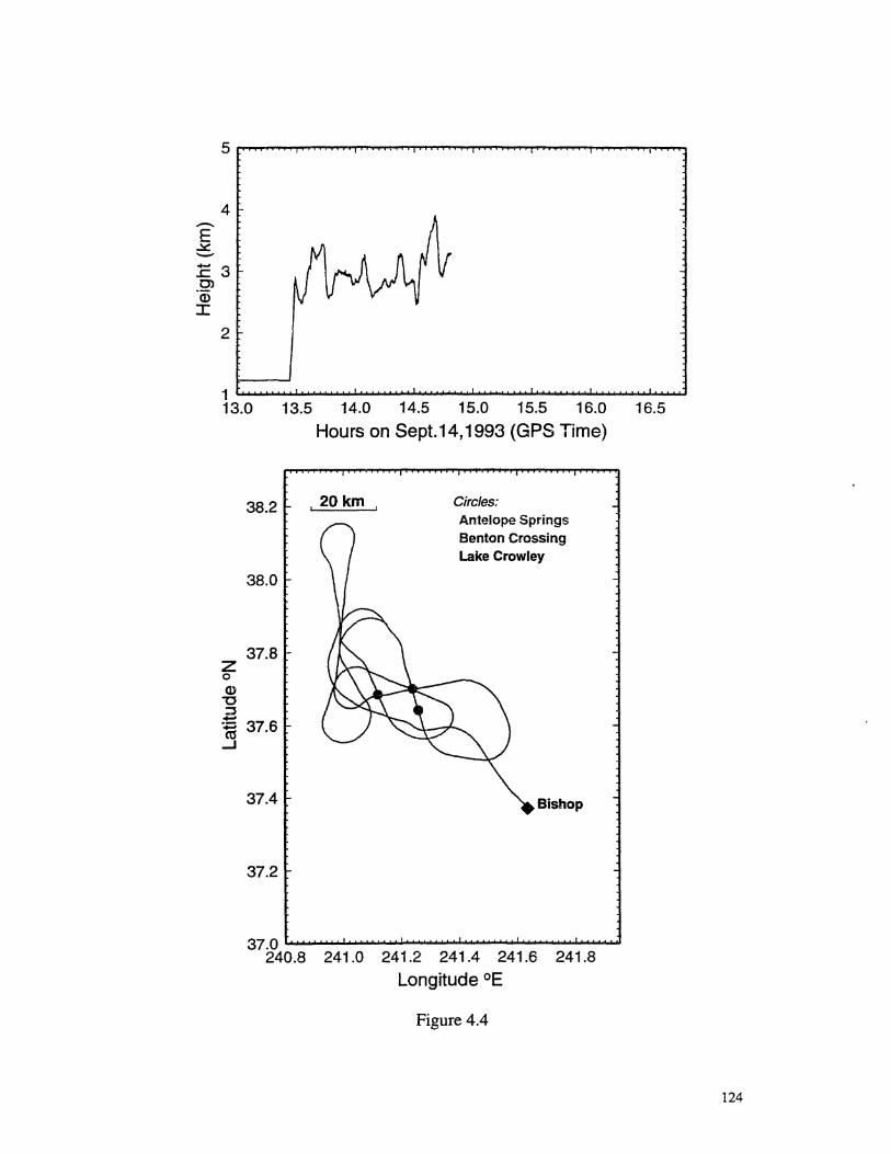
4

2

1~""""'''''''''''''''''''''''''''''~~~''''''''''''''''''''''''''''''~''''''''''''~''''''''''''''''''''''''''''''''...w..I.''''''''-'-I.''''''''''~.u

13.0 13.5 14.0 14.5 15.0 15.5 16.0 16.5

Hours on Sept.14,1993 (GPS Time)

Circles:Antelope SpringsBenton CrossingLake Crowley

,20km

38.0

38.2

37.8Z0

CD-c~~

37.6;:;as-J

37.4 Bishop

37.2

37.0 .........~..........................................~.................~~...........................~""""""'"240.8 241.0 241.2 241.4 241.6 241.8

Longitude °E

Figure 4.4

124

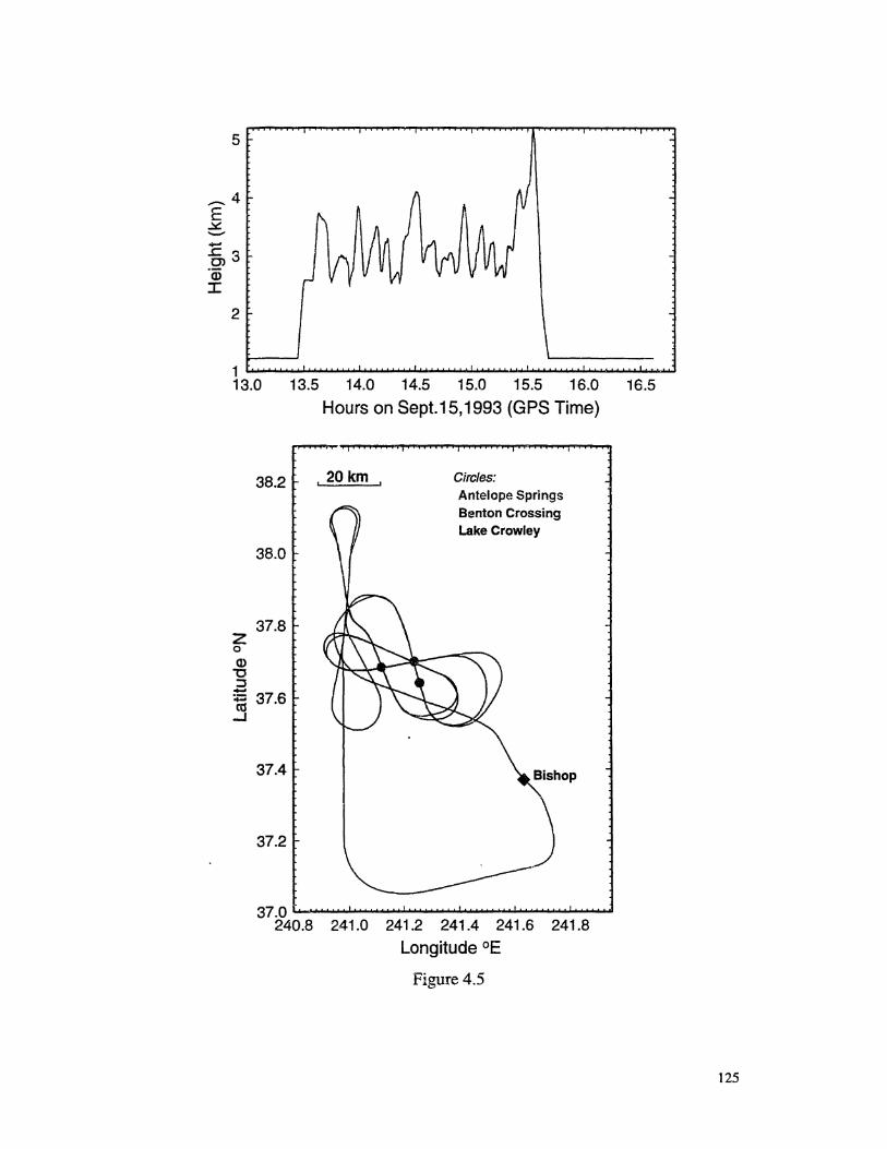
5

1~"""""""""'''''''''''''~~''''''''''''''''''''''''''''''''''''~~''''''''''''''''''''''''''''''''''''''''''''''''''''''''''''''''''''''''''~1.&.I

13.0 13.5 14.0 14.5 15.0 15.5 16.0 16.5

Hours on Sept.15,1993 (GPS Time)

38.2

38.0

37.8zoQ)-c::J

;; 37.6ca-J

37.4

37.2

, 20km Circles:Antelope SpringsBenton CrossingLake Crowley

Bishop

37.0~"""''''''''''''''''''''''''''''''''''''''''''''''''''''''''''''''''''''''''''''''''''''''''''''''''''''''''''''''''240.8 241.0 241.2 241.4 241.6 241.8

Longitude °E

Figure 4.5

125

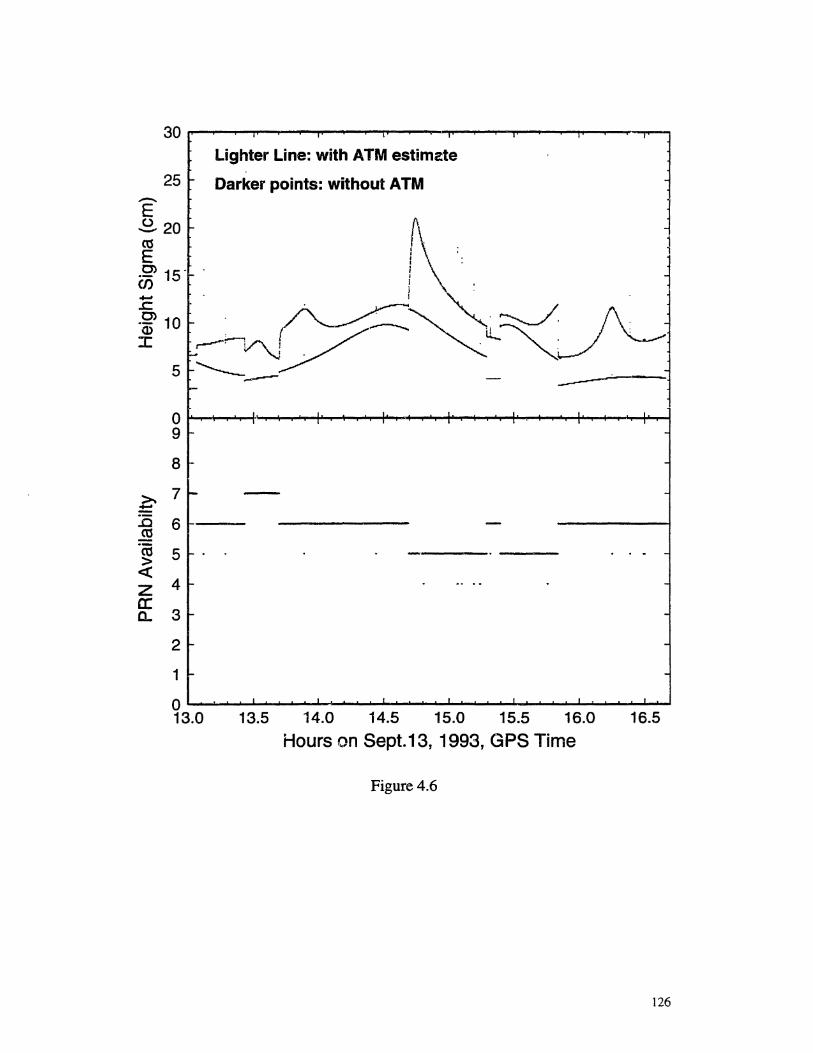
Lighter Line: with ATM estimate

25 Darker points: without ATM

~ ~E~20~ ,E

.0> 15·en+-'.cC).- 10Q)

:c5

13.5 14.0 14.5 15.0 15.5 16.0 16.5

Hours on Sept.13, 1993, GPS Time

09

8

~7

.:!:

.c 6!Q-(ij

5>«z 4a:

3a.2

1

013.0

Figure 4.6

126

16.514.0 14.5 15.0 15.5 16.0

Hours on Sept.13, 1993 (GPS Time)13.5

42o

-2

-4 E-+-+--+-+-+ ....-..t~ ....-.4~-+-......-I~ ~!--+ --t--+- .-....42o

-2

-4 ~-+--+-~!-+-+--+-......,.-+-.............-..4~-+-~J-+.o-+--+-~ ......-+-~I--t-......-i-...--.--t-.............

42o

-2'-""-454~--+-+-+.....-"""-"""'-+-.......-+-+-+.....+-+........................~-+-....-.+-+-+-+ ........-+-+.................-li

-- 2 PRNC;»9 ~t. • " .'.b .'. • j;.if, ~C/) :; ~ c-:'." ~l·~ .~tn:"', ~ .itt... It,.. ," • ..~.iS ":,.... ·~li" ~~ "ca 0 i..\..~~-tt.~ .. h~~(.,.C't;'#.~J;";; .,::~. ·~·~~~,,-~v~~~ ".. ~I-.: ~.. -«-----\r'..::] .. ~~, '" ~. ~:o/;.:- .:~ ... ".~ :. r" .." I 0 •• " ":ff-c -2

.~ -4 ~-t--+-~I-+.............-+-+......-+-~~-+--t-l..............-+-........-+-...........t-+~,~.............--~a: 4

2 · .". "~.~ -:,.' ~ l~ \.. ,. } :~.. ~- ;,:" ~ ..,i.:. .o!. .. ~';f~~' ".. .. ..o .~~~~~~'·!";1 ••~~... • *,fr::.f:.~·~"'" i'f~d::~.~:r.:t""~ir;' ;.!=~A~, ::.t:-;;.-: !':.~~~~"-.~.•t- .... ,...t$t .<.~.. ~. .,.~.; ,a ~ .' ." to,~ lL"- :.1 or' ·.c...;'·1.~ ~ ~ ~.." ·rr ~)I!'t-2 ' ..". A:. ' , .. ..,. or ~". • ': ~. • -rtr-"( • .. • -

-4 ~-+-............+--t~-4--t-+-+"""""'~~-+-""-""""--+-...-f-- ........................~__-.........-.~.......-:a42 ..~ .

.. .L': .~.~ ,~ zt....o ~~~~~1'~~/~~?·:..~~J\i·\tF!",fi"· \%'; ~:.~~-..,. ..• ;:.......... '.~ ¥.~: .. ... • ....

-2-4 ................42o

-2

-4 ~-.........-........-...-+-.......i--+-......+-...-.+-+-~......-+--4-0...............-+-~.....................a.....-t-""'-.........:I42o .

-2-4 ~ -'--............... .........~......-'----.--I........................... ........ .....-. ..............-'--'--'-.-.....................,;,

13.0

Figure 4.7

127

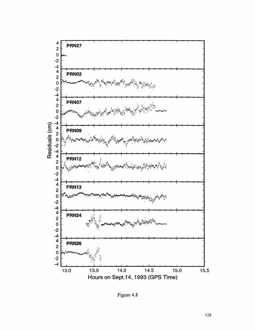
PRN02

PRN27

.... ~

._ ':1;"i!f~~.;~l;.~: .. ..t~

.~.:;~~. .~~

42o

-2

-4 E--+--......-t--+----+----t---+-~......__+o~__t--l~t__..--+___+_~-+-_+__+__+.......__+__.~~42o

-2

-4 ~ot--+_+-........-+--+-__+__+........~___t~l--t__+__+__+_ ............._+__+_........__+__+~~......_:J42o

-2............ -4t 4~t--t-..+..................................--+--+--+--t---+-..............+-+--.....-+---~~--+--+--+-~

'-"'"2en(E 0-5 -2

om -4 ~+--..__+_..........--+--+-_+......__+__t--l~+__+__+_ ..........._+__+__+__+__+O__+__l~~ex: 4

2o

-2

-4 ~+--+___e_-+--+--+-...............__+__+......~~............+__+__+_......................._+__foo__+__l~~42o

-2

-4 t'o-.....-+--+--+-......-+--+.....~p...-+--+-.........................--t--+--+.....-j~+--..-.-+--+- .....-+--!I42o

-2

-4 ~t+-...--+--...........-+-~--+-.....-..-----I~I--.....+-~............-..-+--+--+-..............--I-I-~42o

-2-4 ~............ ..............__--'-............ ............. .....__111111.:- ........................... ~___

13.0 13.5 14.0 14.5 15.0

Hours on Sept.14, 1993 (GPS Time)15.5

Figure 4.8

128

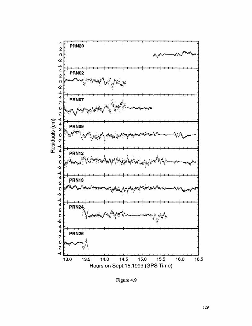
16.513.5 14.0 14.5 15.0 15.5 16.0

Hours on Sept.15,1993 (GPS Time)

2

42o

-2

-4 ~"""+-~"""~'-+"""""""-t--+-......-t~....-+-+-t-.............-+-.....-.................-....................-~42o

-2

-4 ~"""'-+-"""-+-~l-+ ~~-+-~~-+-+-t-+-"""'~'''''''I-+1 ' -+, ~4

o-2

..--....-4s:-+..................-+-r+-I~-+-~~-+-~I-+ ......+-t-+-......+-+--+--+-+-+............+-+-+-o+-~5 4""""'2UJco 0-5 -2

.~ -4 F-+...........-I-+~-+-ll-+.....+-4I-+-+---+-li-t'"......+-t-+--+-+-+......-')-......--+-.....+-+-+--t-...-..:Ia: 4

2o

-2

-4 ~....-.......--t--+-~-t- ....-+-..;...-=~-+-+-I............t-+-+-+-t-+-......+-+.....~~---+-~42o

-2

-4 .-+....~......-+-+-+---+-.......t-+-+--+-I-+-;......-+-4-+-.;-........-+-....-.,t-+......-+--4-+--+-.......~42o

-2

-4 ~-+-.............-+-t-+.....+-+.......-+-+-+.........-.-+--+-t-+'-+-.......-T"-t-.......-+--t-t~-+-~42o

-2-4 ~ ................I.-......-""-.......... ..................__...a.-.............'"'"---"......~.......................-.......-..--....01

13.0

Figure 4.9

129

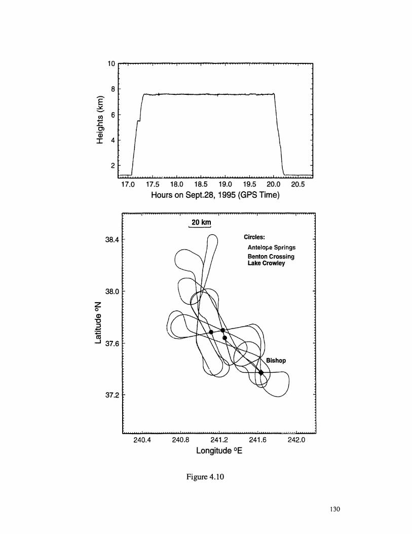
17.0 17.5 18.0 18.5 19.0 19.5 20.0 20.5

Hours on Sept.28, 1995 (GPS Time)

20km,

38.4

38.0

zoQ)'"C::1...+::ttS..J 37.6

37.2

Circles:

Antelope Springs

Benton CrossingLake Crowley

240.4 240.8 241.2 241.6

Longitude °E

Figure 4.10

242.0

130

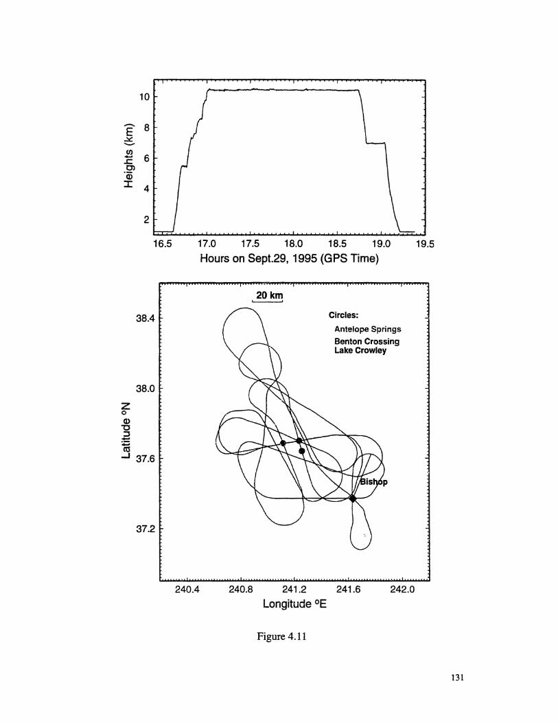
10

....-... 8E~........,.en

6........c:C)

·CDJ: 4

2

16.5

38.4

38.0

ZoQ)-c::1.....

+=ctS

..J 37.6

37.2

17.0 17.5 18.0 18.5 19.0 19.5

Hours on Sept.29, 1995 (GPS Time)

20km,

Circles:

Antelope Springs

Benton CrossingLake Crowley

240.4 240.8 241.2 241.6

Longitude °E

Figure 4.11

242.0

131

15.5 16.0 16.5 17.0 17.5 18.0 18.5 19.0

Hours on Sept.3D, 1995 (GPS Time)

38.5 20 km

38.0

37.5ZoCD

'"'C~......,~ 37.0-'

36.5

36.0

Circles:Antelope SpringsBenton CrossingLake Crowley

241.0 241.5 242.0 242.5 243.0 243.5

Longitude °E

Figure 4.12

132

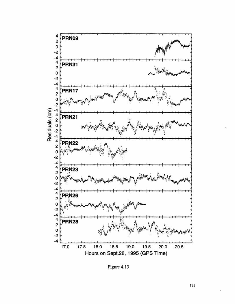
4 PRN09

-~ ~~-4 t+-+-+-......-.......'""i-.......-+-..................~............-,~~~~~~t-+--+- ........~I-+--+-t-+-~42o

-2-44

H-.......-+-........-+-........-+-.......................~t-+-~~~I--)-~t-+-~~.~!'f-to-+-+-+-+- .............-~~

PRN17 .~..:~ o~~

2 ~ ~~t: • •\ {'\ .:' • ,.;....'0 :":,T' ~ ~', ~"{/':o,~ • \. '~. ~ :<~. ;.' .o ~. .~, .It... ~ ..~~. 0,: !. '. ~:~( ~~~A..l/oJl".· ~.?"o "~.y. ...A-,...

~~J '4ttJ!if ~i ';l' "!j' ~,.. ~;:. "" ....." r -.-2 l.· ~':? ., .(. Of" 1 ':: 'r.~f'I'!'i

E -4 H-......-+-................-+.............-+-..........................~-+-................................-+-...................-+-.............o 4...........ClJ 2co 0::J

~ -2Q) -4a: 4 H-...........-I~.......-+-....................~~..............+-+-+-~-+- .......~t-+-.....-+-+-+-+-.........-+-iiiI

PR~N22 ".. :" 1\ .2 .. ~ '.:>' ". ~4\ f:;:- :?.:c..t:":k 1 '::.. .' ~ :

li\ • .r;""4..~. V·1t.,~{· .-~ -. '"-. _l:~'~ ~o \~::' ..v· ',." r ~~o"'. ....'" '~l ~! ••• fJ;:.;.... ~ _. ~.- ..... \,;...,/! t'.':'"'.

-2 -: ° e. ~ :..0 :~.ti- ;:'::

-4 H-+-+....................+-+........-+....-.......-t--.......~........~~-+-.......-+-..............................q-a.......~42o

-2

-4 ~t-+......+-+--+-.......-4-.......-+-e-+-...-~~................................-+-.......-+-~......................~42o

-2

-4 Ii+- ....- ....-P ~I-+-~~~ ....-~ ~42o

-2-4 ---. ""'-'- .---. ..-....- --.... ___..........

17.0 17.5 18.0 18.5 19.0 19.5 20.0

Hours on Sept.28, 1995 (GPS Time)20.5

Figure 4.13

133

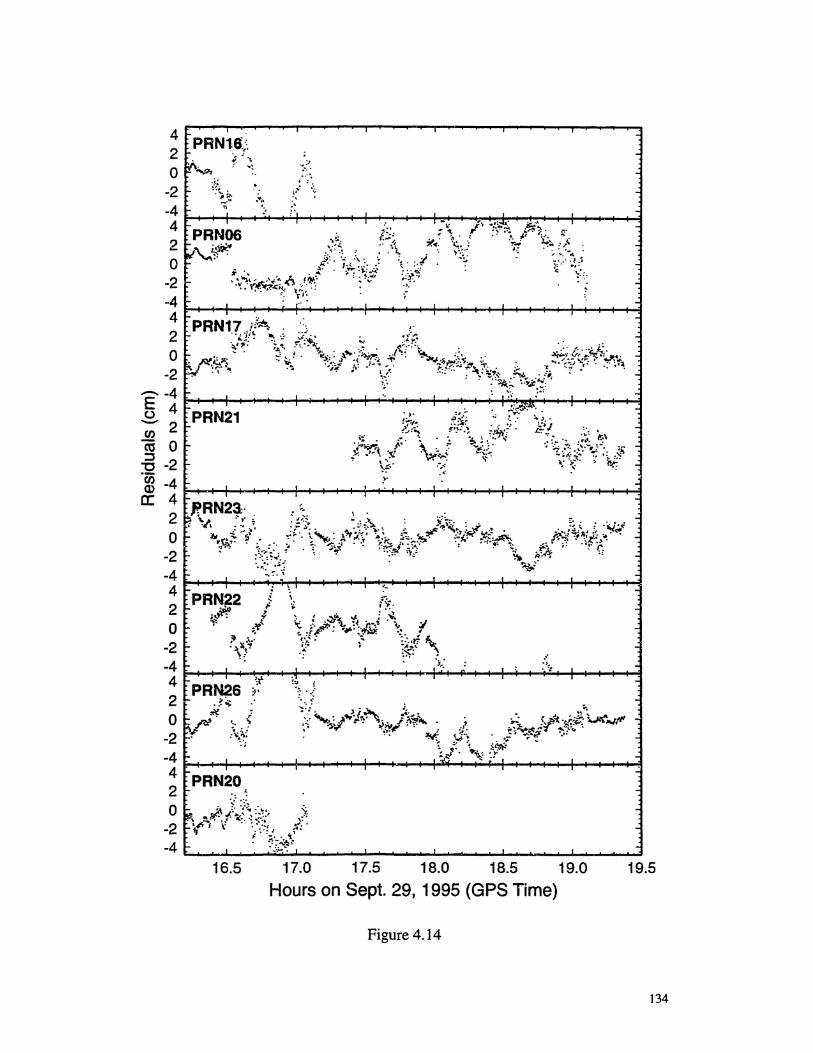
'0 •

.\~~li;~~:. \~if It·: :';! I f: .I .~"-i~~.

42o

-2-442o

-2..44 ~-+"""""''''''''+-4f-+-+--+-O+-~''''-+--+-+-'''''''''''''''''''.''''''''''''''~--+-+-'''''''''''''t--+--+o...:ll

PRN17 .i:'~~·~ !"

2 /J.!~ \~ t.~;'~... "..... ..j.. ..I<..r~:... ...:,. :.,. ;'....' j..:.O -... ~ ~~. ~1.Y"#,..JI·~••: 4..:." ~. :>.~• ..).(:~..,. "~'1}i':t'~.";.~' ... ,=. • ..,.,

_ ~~ .~ ";1r"' .\' )- \{ t.:;-(.. ,. ~~!~:~('f.;'.'i,i;'.(i'! :' ..:. ; ..

5 4 li-t-+..........-......'f--oI........-i-......-t-......................-)...-......-+.......-+-......~,...................+-t--+ ..;;I

'-'" 2 !=:-~~CIJ i,... ?J=,

CO 0 .;~";·rA ./' \,:-..{-6 -2 \~" .-..:

'm -4 ~~..........................+-.......--+--+-.....-i-........~Io-+-+_..+-t.......-+............-+-+--II--+-+......-t-......

a: ~ .,P~N2~: ~ : ~:. \ . ....,..~ .'•. -, :,~ ...}. ~~~\.~.. ~i~.. :..... • :~ i ; ''l4io :tJt ":""rl ••~·.',,'·1?t;,.~·:.\ :"':.~~ ..,.,.:#'~_.~ ~!:::.:.,,'.,.~

-2 .~~": . :~:...,~:;.~~. '\ -i-.,f· '.! !-~i~tY :-$,' ~.,:~ \~ ~~•• ;"~ .t·~rl

-4 ··r.·~-:·.:.·f ~

42o

-2-44~.................-~t--+ ..........-+-....-.t-+.............-~t--+ ..................+-+......................-I~.....-+-~

2~o ,: ;:: \.. ,z;~ .~~;j} \.A"M'";. ~ ...~~~' "'~~. ~

-2 :\::~; . .i· ...;..~ '.~: .,4

..~~ .:;~- ~~..........................-t-~--+..................-+-~~......~-+-.......+-...........................+-~~~42o

-2-4 '"'"- -'-__ ....., __ -lo "- -..........

16.5 17.0 17.5 18.0 18.5 19.0

Hours on Sept. 29, 1995 (GPS Time)19.5

Figure 4.14

134

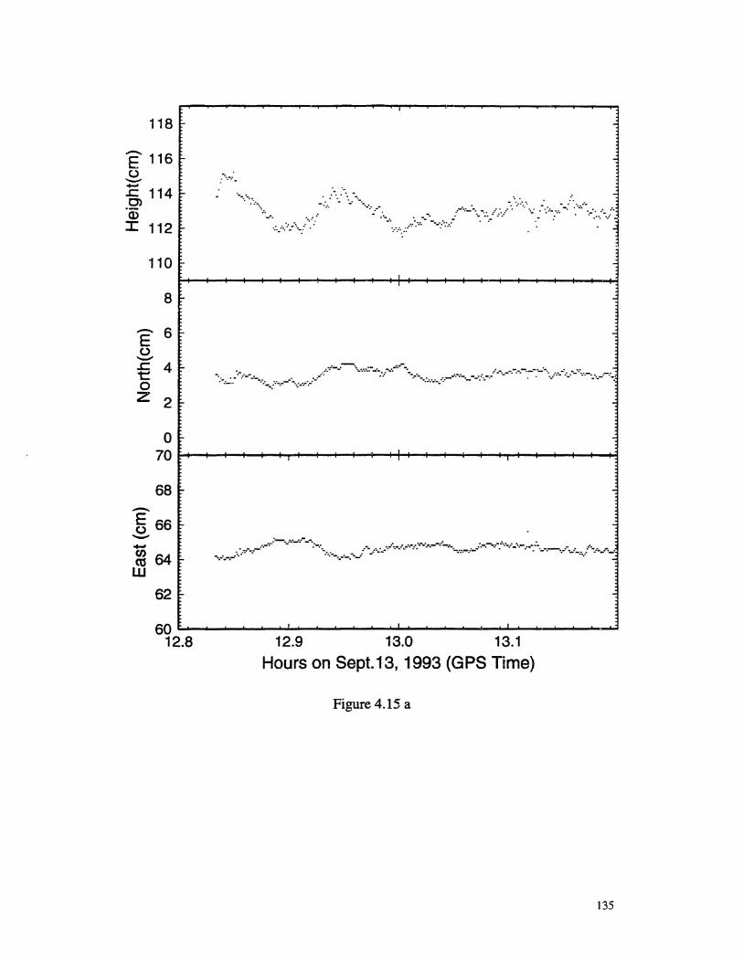
118 - -

-E 116 -u............+-'

..c: 114 ­0)

·CD:I: 112 -

110 -

.....ltil

.:.....:.._..···.oo:·· ••

'. .. '. 'oo' --'•••••, .oo_ .-....--".-':......:.................... :............ -••..:':..:

I,

-

-

8 -

...--... 6 -E0'-"".c 4t::0Z 2

..: -... .••..•..:.-.:- -•..: - - -•••••.....__.•..- -. _ -.-..__._- _•....- .-.-_ .._.. _fl._ __ _.. _ . _ _ _._.._" __._.:•••.:.~. .' - ··-·.·••_-:•••-.--_·....:••••••oo:··..

o70 1-00+-.......-.+-.-+-.............., ..............-+--+--+-.......-+:......-......-+--+--+--+-.......I ......--+--+--+--+-t

68

•••- :-._••~_•••- --':-., • ..' -- --:'._~ _ •••••_ •••__•••-.-- ~"..,.-••-.-. U .-.

-.._.oo_..r\· • ·- :-_ _:._ :.... •• • ••._-.- _.--••••.: J _.

12.9 13.0 13.1

Hours on Sept.13, 1993 (GPS Time)

62

60 .......................... ....I __....r--~......................I ....... .......- ........I __........ ~~

12.8

Figure 4.15 a

135

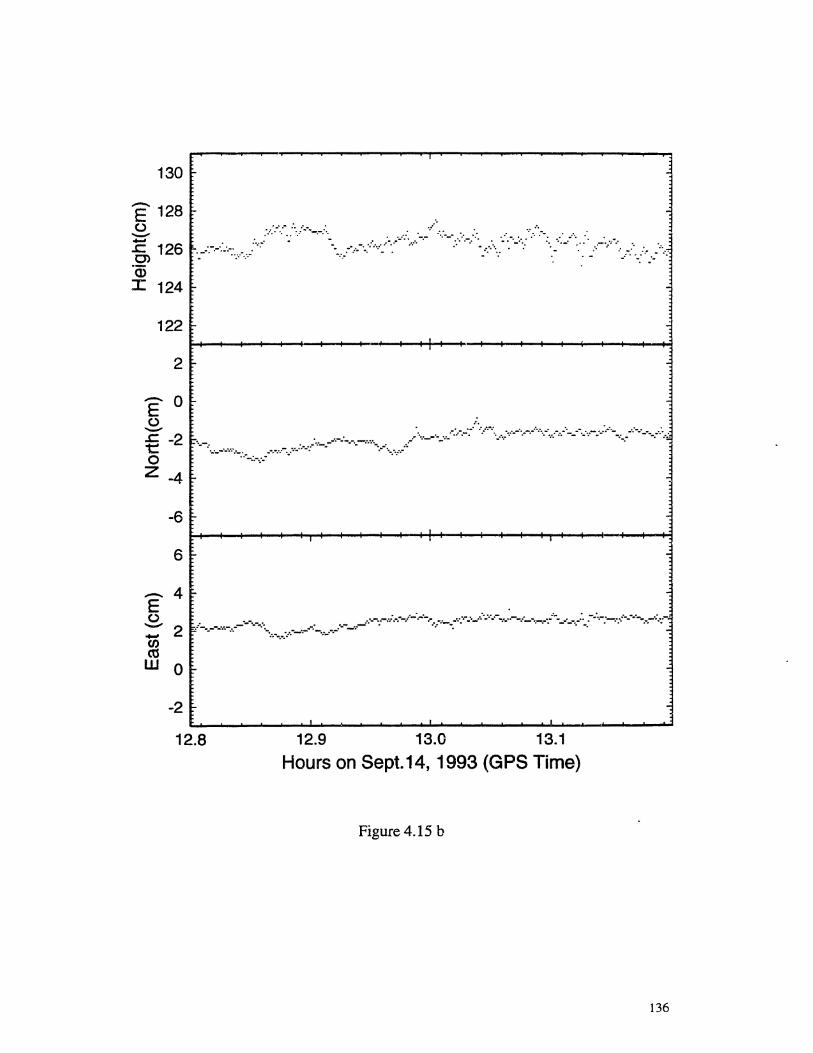
r

130 -

....:-./., ......-:". ; .... :.....:

. ........_•...: .' ..................

..•.." _-- .

E 128 -~ :",:."":-.:•...:.......-.-:...-§, 126 .- . .. ....; .....:.....-..:........~.:....:.: ........ -.-.0)

J: 124

122 ..:

, I I I I I

2 - -

~ 0-Eo~.c 2 -.:. .. : - - : -..--..-.- - : -- ..- "..-.. . ..'.-:_ .. _... ..: __.__...•t _ -..:.._:.-_.: _-- .. '.. .. : .o __ -: -:.-.:..-

Z -4 -

-6 -I

6 -T 1 I

~ 4-Eo ... .._-..- : --..:-.--.- : __ -: -:.: - --l_-.._.-··..-__.__..-.._..- -:-..:- _- -.: -.~ 2 ....-....--......-...--- .......:.... ..- --:. .-.-. :l.--..-..-.- _.-.- --t.'

enasw 0 -

12.9 13.0 13.1

Hours on Sept.14, 1993 (GPS Time)

-2

12.8I I I

-

Figure 4.15 b

136

-92 ~ .,.'J' • ..

J

-

-94

-96

-98

-100

-18

, ..- .

'..'. ­....... ._-

'.'

................

-.'

., I

I

':-."

-

-

e-20o..........

.I::. -221::oZ -24

, . "...-.,-.:.:-- .: ...-:."... u.:..'.'- '.'" '",:':... .' ...•..............

...........

... .-' .:::.. .. ......-......- ......-.....:...•.•...... :'.

:'-.:::' ....". ~.......-

..- It.·......... ".:._:. • '.r" • ''-

. -.:-....:

-

-26I

120 -

,I

.' _... ".

I

-

-

_ ... .­..- . .-........ ...... -..... ". -. -- .. ,... ....... .-

11-.. .." .,. - . .-..- -

E 8 .: :..: : . -_. ..:, -. .", '.. .'- '" -. 'J ::.::·..n: ._-:, •.~o .. - -_.:- "::..' .- - -..,'::: 116 ~":-"" . A/::··:··:···::: . '.. ·tI'J '-': •. :'-~".:"~ .~J'

W 114 -

112 -I I I

12.8 12.9 13.0 13.1

Hours on Sept.15, 1993 (GPS Time)

Figure 4.15 c

137

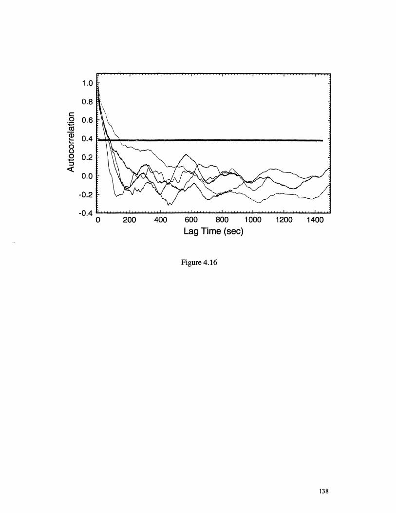
1.0

0.8 \.\

c:: \.0 0.6

"

;; \ctS \

03 0.4 '"'-L-

a00 0.2.....,::J«

0.0

-0.2

-0.40 200 400 600 800 1000 1200 1400

Lag Time (sec)

Figure 4.16

138

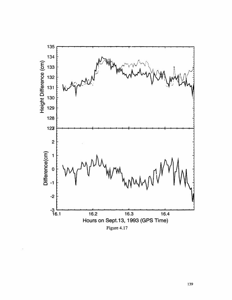
16.2 16.3 16.4

Hours on Sept.13, 1993 (GPS Time)Figure 4.17

-3 ......__...... -.....- .-.-..............__---........ "- ~...................._s_ ........

16.1

....---.E 1o'-""a>oc: 0~Q)"I­......is -1

128

-2

2

Q)

() 132c:.(1)'-

.S:? 131~

o...., 130.!::0>

·03 129J:

139

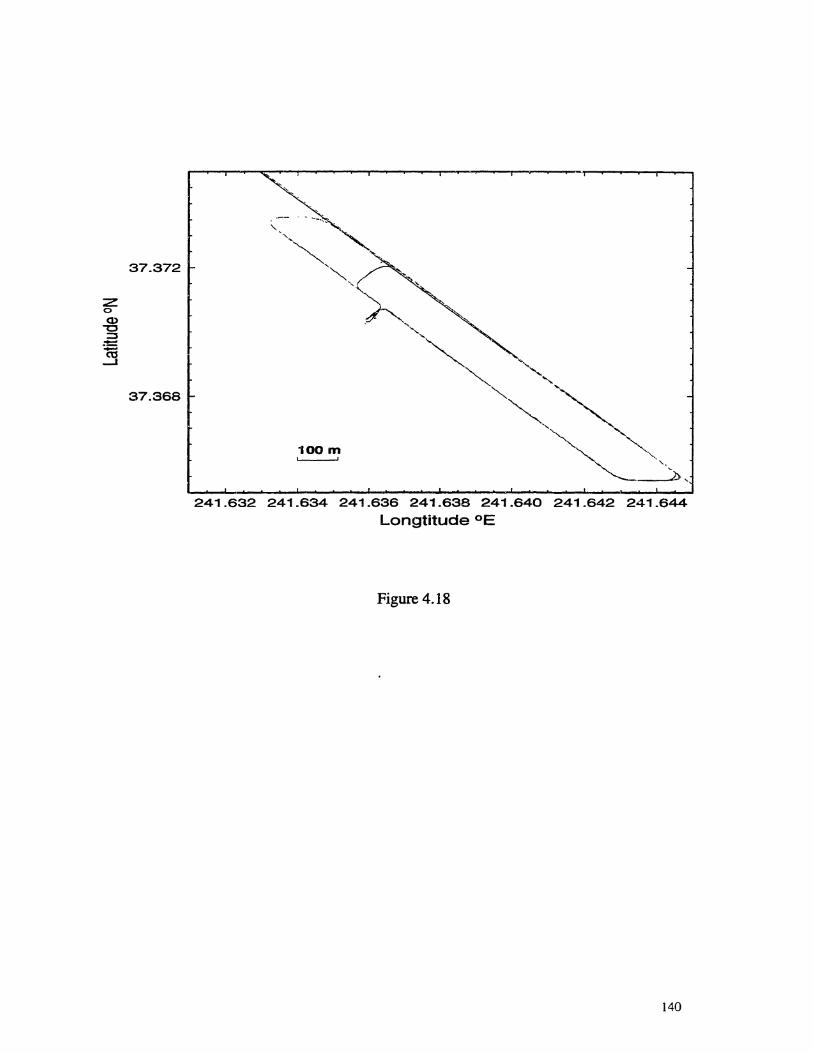
37.372

37.368

100 m,

241.632 241.634 241.636 241.638 241.640 241.642 241.644

Longtitude °E

Figure 4.18

140

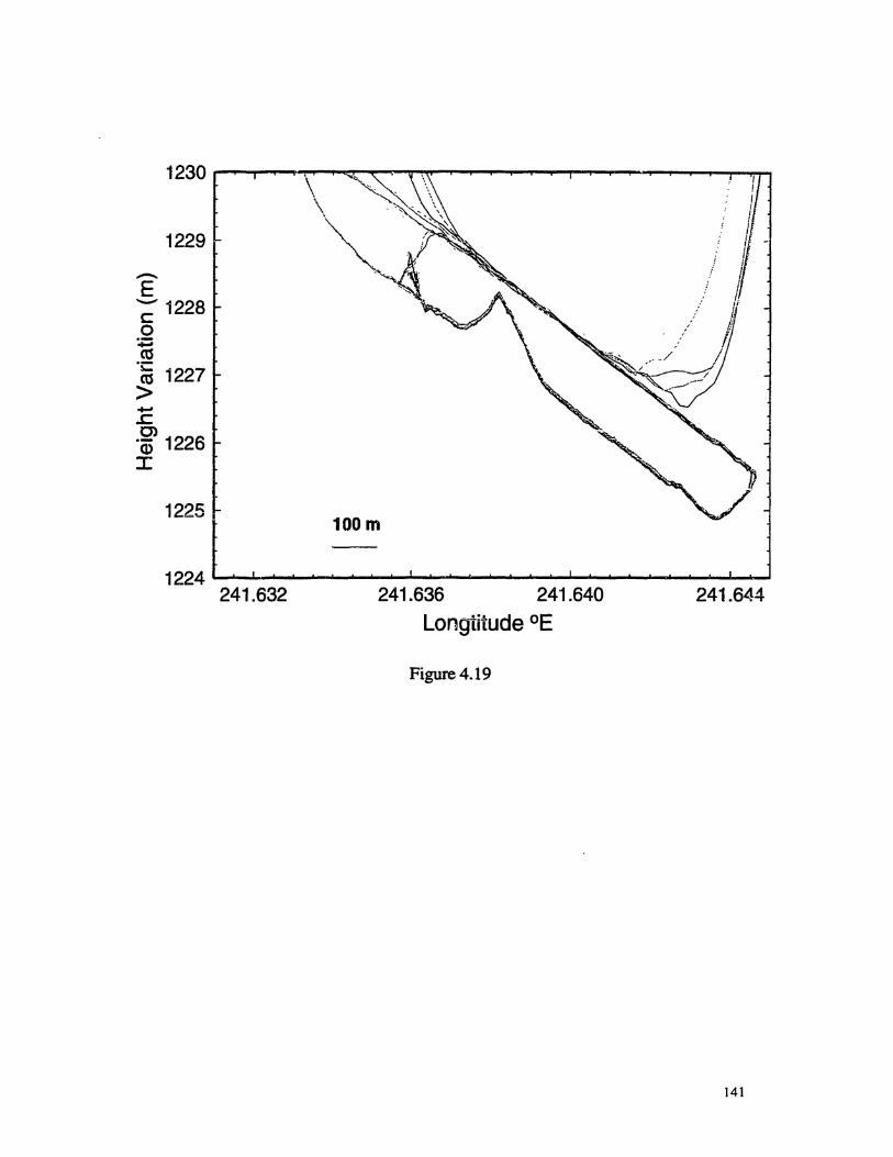
1229

~

E-; 1228o

:t=ca"(ij 1227>+oJ.c:0>

-Q) 1226J:

1225100m

241.632 241.636 241.640

Longtitude °E

Figure 4.19

241.644

141

1229

.,...........E 1228

'--""

c:o15 1227-;::ctS>.E 12260>

-CD:I:

1225

241.638 241.640 241.642

Longtitude °E241.644

8

6

~4

ES2Q)oc:: 0Q)'-Q);= -2o

-4

-6

-8

600 800 1000

E-W distance (m)

Figure 4.20

1200

142

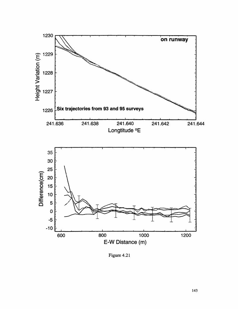
E 1229"""-"'"

c::o;;co 1228-i::m>......s=..0) 1227Q)

:r:

1226 Six trajectories from 93 and 95 surveys

..........

on runway

241.636 241.638 241.640

Longtitude °E241.642 241.644

35

30

25,-.,-.

E 200"""--'CD

15(Jc:Q)

10~

CD

==b 5

0

-5

-10

600 800 1000E-W Distance (m)

Figure 4.21

1200

143

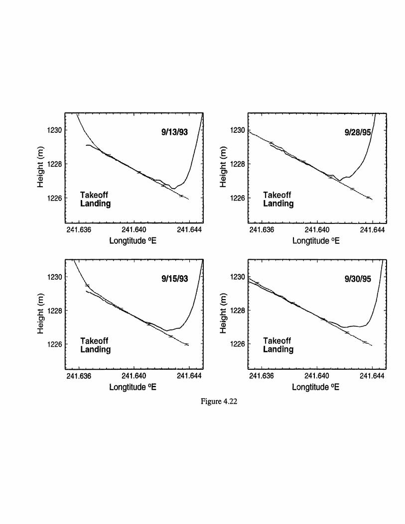
1230

............

E'-'"

E 1228OJ'm::c

1226 TakeoffLanding

9/13/93 1230

...--...E

"'"""E 12280)

'CDJ:

1226 TakeoffLanding

241.636 241,640

Longtitude °E241.644 241,636 241.640

Longtitude °E241.644

1230 ..

...-...E

""-'"

E 12280>'m:r:

1226 TakeoffLanding

9/15/93 1230

,-...

E.............

E 12280>

'CD:c

1226 TakeoffLanding

-t241.636 241,640

Longtitude °E241.644

Figure 4.22

241.636 241.640

Longtitude °E241.644

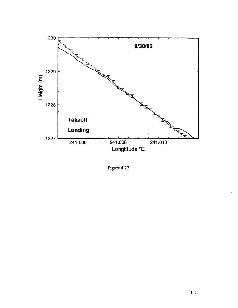
1229

1228

Takeoff

Landing

241.636

9/30/95

241.638 241.640

Longtitude °E

Figure 4.23

145

Chapter 5 Validation ofGPS Trajectory from ATLAS

Measurements

In this chapter, we address the quality of our trajectory by evaluating the GPS trajectories

on the flights using the results obtained from th~ laser measurements over a flat surface, Lake

Crowley. We use the laser altimetric results as an external data source to valid~~te the trajectories

because it is impossible to be done by GPS measurements themselves without the fixed marks

for re-occupation. Another main goal of this chapter is to detennine the improvement to the

altimeter results through the use of our trajectory. The aircraft trajectory provided by GPS

kinematic estimation is one integral part of entire airborne laser altimeter measurement system.

and it is important to investigate the impact of GPS trajectory's accuracy to the precision of

ground laser measurement of ATLAS system for calibration reasons.

5.1 ATLAS Data Analysis

The laser data used in this thesis were obtained by the NASA T39 jet aircraft during the

1993 surveys. T39 jet aircraft was equipped with the "Airborne Terrain Laser Topographic

System" (ATLAS), two GPS receivers, a Litton LTN92 inertial navigation system (INS), and

both video and still aerial cameras. The ATLAS was developed in the last decade by NASA for

altimetric surveying. It is a low altitude ('- 500 meter) nadir-profiling altimetric laser system and

yields a single surface footprint line with footprint radius of 0.85 meters on the ground in 1993

Long Valley survey. The sampling interval is set such that the footprints are approximately 2

meters apart. Because the laser port is fixed to the aircraft, its footprint on the ground will move

off-nadir when the plane rolls or pitches. The INS is used to measure roll, pitch, and heading in

order to locate the laser footprint in the post-flight processing. For more technical details of the

ATLAS system are given by Krabill et. al., [1995]; and Ridgway et ai., [1997]

We provided our new 1993 GPS trajectories to the SIO team who conducted the ATLAS

data analysis in the same way as their previous data analysis [Ridgway et al., 1997]. The surface

height measurements of the laser footprints were returned to us for further analysis of aircraft's

147

trajectories. Our main purpose for this test was to validate the GPS trajectories, so we use only

the laser height measurements over the flat surfaces such as Lake Cro\vley and the Benton

Crossing.

5.2 Calibration over Lake Crowley

Lake Crowley is one of the four regular targets for tlle topographic calibration

examination during the 1993 Long Valley surveys (Figure 5.1). The large flat surface of Lake

Crowley is targeted for data calibrations in Long Valley surveys [Ridgway et al., 1997]. Due to

the periodic spilling of the water through the dam, the surface height may vary every day.

However, changes in water level of the lake are available from the tide gauge ineasurements. For

the 1993 surveys, we used the tide gauge measurements records from Ridgway's [1997] Figure 9

(1997) to adjust the lake surface heights. The lake surface height changes are -5.0 cm for the

Sept. 14 flight and -8.5 em for the Sept. 15 flights compared to the surface height recorded in the

Sept. 13 flight. There are data available in two over-flights of Lake Crowley on Sept. 13 and 15,

but only one flight on Sept. 14 due to the failure of GPS clock at the Bishop base station during

the later flight section. All five elevation measurements over the Crowley Lake are shown in the

Figures 5.2 - 5.4. In Figure 5.2, we show the results from the two flights on Sept. 13. For each

track, we estimated a cubic polynomial line to fit the data. The cubic polynomials from both

tracks have the same shapes and are offset by a consistent 0.8 cm over the 4 kIn plus track length.

The difference is consistent with the increase of lake surface recorded from the tide gauge station

during these time. We used a spline interpolation and 5-point moving average to smooth out the

high frequency variations and show the results in the middle plot of the Figure 5.2. We plot the

elevation height over the ellipsoid of aircraft over the Lake Crowley in the bottom plot of Figure

5.2. One flight is nearly flat while the other has 50 meter height variations. Although the

trajectories of the two flights are not the same, the estimated topographic profiles of Lake

Crowley are all close to each other everywhere. The RMS scatter of the profiles around the

smoothed surface are 2.5 and 2.4 em for the fITst and second tracks, respectively. The measured

swface profiles have slopes of 3 cm/km which is a little less than the local geoid slope (4 em!

km). However, the cubic like profile indicates that the strong wind on that day may have caused

148

the long wave variation and result in the water level deviating from an equipotential surface

[Minster, 1998]. The steady wind pressure could cause several centimeter level change in long­

wavelength in the water surface.

Figure 5.3 and Figure 5.4 show the other flights over the Lake Crowley on Sept. 14 and

15 surveys respectively. The measured surface profiles are ',ery flat with a nearly constant slope

rate around 4-5 cmlkm which is close to the local geoid slope (4 cmlkm). The mean difference

of the Sept. 13's and Sept. 14's measured lake heights is 5~9 em comparing to the 5 em, the

height variations obtained from the tide gauge observation. The mean difference of the Sept. 14's

and Sept. 15's measured lake heights is 3.2 em in a good agreement with the 3.5 em, the tide

gauge results. In Ridgway's analysis of the 1993 ATLAS experiments, the second track of Sept.

15, 1993 (the fifth) has a 10 cm bias and the errors in the GPS trajectory were thought to be the

cause. In our analysis, we have an approximately 4 cm variation in the middle section, but the

second track agrees with the first track on the Sept. 15's in the beginning and end section (the

middle plot of the Figure 5.4). We do not see a constant 10 em bias in the fifth track. These new

results indicate that part of errors in the former data analysis may be due to the failure of the old

software to resolve correctly cycle slips and ambiguities during the flight.

We calculated the autocorrelation function of the differences between different tracks

over Lake Crowley. The results are plotted in Figure 5.5 as a function of the distance along the

lake in north-south direction. The autocorrelation length (lie) is under 5 m. With an aircraft

speed of -80 mls over lake, the time autocorrelation length (lIe) is under 0.1 second which is far

smaller than that of GPS correlation time (70 seconds). The RMS scatter is also much larger than

the GPS positioning RMS scatter (2.5 em of ground track heights vs. less than 1 em in GPS

trajectory during less than 2 minutes). these results indicate that most of the errors of the laser

measurements are at higher frequencies which may not be from the trajectory-related sources.

In order to investigate the effect of GPS trajectory on the topographic determination of

the airborne laser altimeter, ""'e plot the RMS scatter of the lake surface residuals in the five

flight tracks over the Lake Crowley against the possible errors of the GPS trajectories in Figure

5.6. The RMS variations of the lake height from the laser measurements are computed by

149

Sllbtracting their individual height estimates from their cubic-polynomial fitting lines. The errors

of the GPS trajectory in Figure 5.6 are represented by the uncertainties in a\teraged single epocll

which normally rely on the noise level of process noise and measurement noise as well as the

satellite availability. The uncertainties can vary from 4 em to 11 cm depending on the satellite

constellation during the trajectory solution. A 5 em noise level used for GPS system. However,

the RMS variations of the lake surface heights are all around 2 em to 2.5 em for different flights

with RMS from 2.3 to 2.4 em (Figure 5.6). The second flight of the Sept. 15, 1993's survey has a

slightly large scatter which may result from the unknown departure in the middle of the track

(Figure 5.4). There is no obvious relationship between the precision of GPS trajectories and the

laser height determination which implies that errors in the current GPS trajectories contribute a

small amount to the high frequency errors in the height estimates. The results also suggest that a

more realistic value for the scatter of surface heights is much less than the formal error of the

trajectory when 5 em phase noise is assumed.

5.3 Crossover Analysis

5.3.1 Lake Crowley

One important teclmique for assessing the errors in the altimeter data analysis is to

compare the estimated heights at the same location from two flight tracks, a method called as the

crossover analysis. Crossover analysis directly compares the laser footprint pairs for which

centers are within a small search radius. If a search radius is small enough, the footprints should

reveal the same (or close) elevation height. We use the crossover analysis software package

developed by 810 to do the crossover analysis for the data collected in Lake Crowley and the

Benson Crossing sections. The search radius in our analysis was set to the same radiu..c;; used by

Ridgway et al. [1997], 2 meter which yields a large set of points for the statistical test. Figure 5.7

shows the histogram of the cross analysis for Lake Crowley from first four track lines. The

results of the fifth track are not used for the purpose of comparison to the Ridgway's results

(which did not include this track). The tide gauge data are used to remove the time-varying lake

150

surface heights. The tide gauge station is near the dam, which is at the eastern side of lake, and

the variations of the lake surface are under a few centimeter although the wind-driven seiches

could cause some problems. The total number of crossover points obtained from the matching of

the fOUf lines is 276, which is larger than the 215 obtained by Ridgway et al. (1997). This may

inlply that our GPS trajectory determination is more stable. The mean elevation height difference

of crOSSO'ler points is 0.2 em with a standard deviation of 4.5 em. Almost 78% of crossover

points are within 5 em. This RMS scatter is close to the expected value of 3.5 em based on the

RMS scatter of the profile about the cubic fits. The additional scatter is probably due to the mean

differences between the surface profiles.

5.3.2 Benton Crossing

Benton Crossing is at the edge of the Long Valley caldera but away from the resurgent

dome (Figure 5.1). In this area the terrain is very flat with some low vegetation cover; the mean

slope is approximately lcm/m. Figure 5.8 shows the crossover statistical histogram for Benson

Crossing with data from the tracks that cross that spot. When Compared to that of the flat lake

surface, the crossover analysis for Benton Crossing shows longer tails. The outliers are caused by

local rough ground topography. For example, t\\lO laser hits reflected from the opposite sides of

the sharp stream bank edge in the terrain may generate a large range difference. The mean height

difference of 218 point pairs is -2.1 em with RMS of 21 em. After deleting the outliers

(difference larger than 0.4 m), the mean height difference of 202 point pairs is only -0.2 em with

RMS of15 em.

151

References

Hofton, M., J., Blair, B. Minster, J. Ridgway, D. Rabine, J. Bufton, and N. Williams, Using laser

altimetry to detect topographic change at long Valley caldera, California, Earth Surface

Remote Sensing, SPIE 3222,295-306,1997.

Krabill, W. B., Thomas, R. H., Martin, C. F., Swift R. N. and Frederick, E. B., Accuracy of

airborne laser altimetry over the Greenland ice sheet, Int. J Remote Sensing, 16, 1211­

1222, 1995.

Minster, J. B., Private Communication and Discussion, 1998.

Ridgway, J. R., J.B. Minster, N. P. Williams, J. L. Bufton, and W. Krabill, Airborne laser

altimetry survey of Long Valley, California, Geophys. J. Int. 131, 267~280, 1997.

152

Captions

Figure 5.1 Locations of the targeted area by repeat flights for the Long Valley mission (Benton

Crossing, Antelope Springs and J..Jake Crowley) (from Hofton et aI., 1997). Mono Lake is

used for INS bias correction. The lines are the fligl1ts on the 3 days in 1993 mission.

Figure 5.2 The top plot sl~ows the ground heights of laser footprints on the L~ke Crowley surface

on Sept. 13, 1993. The darker and lignter points are the first and second fly-over lines

respectively, with the cubic fits to each fly-over shown with dark and light lines. Sampling

rate is 50 Hz. The middle plot is the smoothed profiles of lake surface obtained by remov­

ing the variations with spatial scale <100 meters. Tht; bottom plot shows the heights of the

air~raft flight over Lake Crowley. The darker line are the first flight-over line and lighter

line is the second in the same day. The sampling interval is 0.5 second (2Hz).

Figure 5.3 Similar plots as those in Figure 5.2 but for the flight on Sept. 14, 1993.

Figure 5.4 Similar plots as those in Figure 5 ..2 but for the flight on Sept. 15, 1993. The cubic fits

are not performed due to the differences in the middle of lake Wllich may result from the

wind pressure or other forces.

Figure 5.5 The normalized autocorrelation functions of the nleasured surface height differences of

Lake Crowley from four tracks. The solid line represents the lake surface height differ­

ences between the second and tile first fly-over tracks on Sept. 13, 1993; the dash line rep­

resents the lake surface height differences between the only fly-over track on Sept. 14,

I993 and the second track on Sept. 13, 1993; and the dotted line represents lake surface

height differences between the first fly-over track on the Sept. 15, 1993 and the first fly­

over track over the lake on Sept. 14, 1993 The upper plot shows autocorrelation functions

in full time while the lower plot shows the details in 0-50 ffi.

Figure 5.6 The RMS of altimeter determination of the Lake Crowley surface versus standard devi-

153

ations of the GPS trajectories. The uncertainties of surface of water level are calculated as

the averaged departure values of the laser measurements from their cubic fits mainly due

to the lake shapes and wind effects. The error bars represents the RMS scatter of the aver­

aged departure values. The uncertainty of the GPS trajectory is the single point uncertainty

of the GPS measurements. From left to right, there are results of the Sept. 15 first track,

Sept. 13 first track, Sept. 14 track, Sept. 13 second track and the Sept. 15 second track

respectively.

Figure 5.7 Histograrrl of repeat pass differences over Lake Crowley using ATLAS during the

Sept., 1993 Long Valley mission. Search radius for crossover collocations is 2 meters. The

height variation of daily lake surface is removed using the tide gauge observations. The

number of cross-over points is 276 with the first 4 flight lines over the lake. The mean dif­

ference is 2 rom with standard deviation 4.4 em.

Figure 5.8 Histogram of repeat pass differences over Benton Crossing using ATLAS dwing the

Sept., 1993 Long Valley mission. The number of cross-o'ver points ohtained is 216. The

mean difference is -2.1 em with RMS 21.1 em. After the outliers are removed (the darker

bins), the mean difference is 0.2 em with RMS 15 em.

154

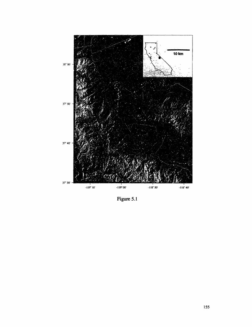
Figure 5.1

155

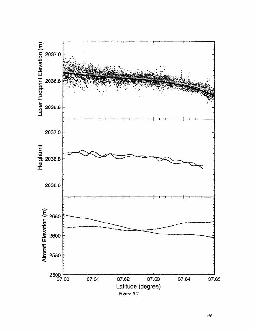
§ 2037.0:t=ctS>Q)

W.....5 2036.8"-Om...,oo

LL'-m2036.6co

...J

2037.0

2036.6

...-...

..s 2650co+:ias>Q) 2600W

=~e 2550

<3::

~....... ".e.,,'.........

-~~~.............-..=......~~~~#........

37.6537.6437.62 37.63

Latitude (degree)Figure 5.2

37.612500 "'---'-.........-.....-__......... .--..-----.~ ........._..._ ~ ......r._ ..........~ ._6

37.60

]56

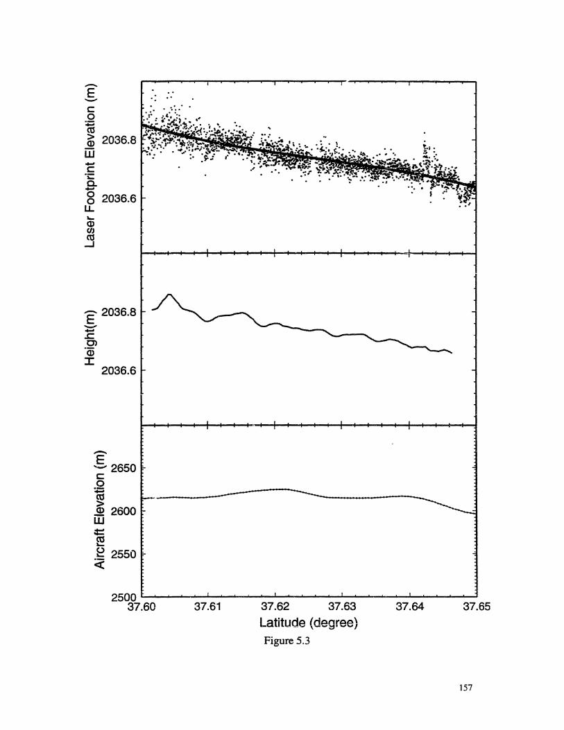
co

+:ica~ 2036.8w~

£::-i::a.....,g 2036.6u..

T

E 2036.8'-"....,.r=C)-0)J:

2036.6

............

S2650c::o+:ias>CD 2600W

==~~ 2550<c

37.6537.6437.62 37.63

Latitude (degree)Figure 5.3

37.612500~ ..........-.-...... .............. ......... ...........-.-...-..r...----"" --,,-,-,,,-,

37.60

157

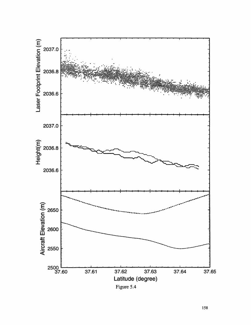
....-....E

"'-""c: 2037.0o

:;:;ctS>Q)

w 2036.8....,c.;::a.~o~ 2036.6

2037.0

~

E"""'--" 2036.8+-'..r:::.en

.Ci)

J:

2036.6

...--...-.

§.. 2650c:o

+:ictS>~ 2600w=~~ 2550~

250037.60 37.61 37.62 37.63

Latitude (degree)Figure 5.4

37.64 37.65

158

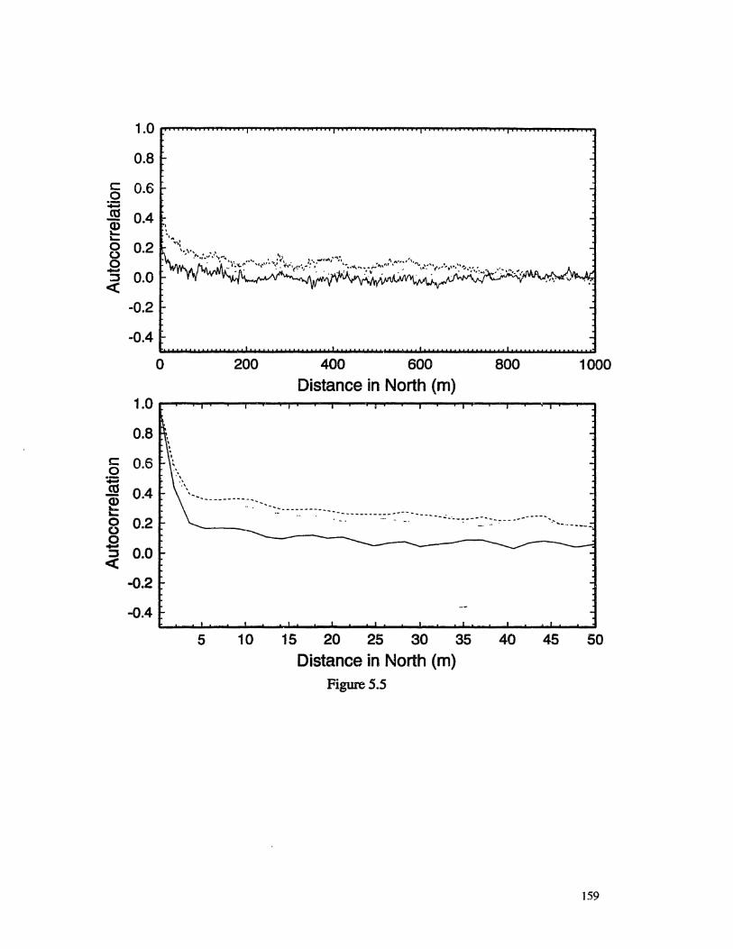
1.0 .........~,....,.,.,~~......,..,.,.,.,.,..~,.,..,.,.,. ............,.......,.,............,.....,...'""""""'...........~~~~~~~

0.8

1000800400 600

Distance in North (m)200

I

'"""''':,....... ~f'.,.,••~\:',,~~ ',\ ~r\. ,

. • ~~r:v.~·""-'~\"""·"'~ ~~"·I(~ ••'J-~"~:-'~""I :'~~"'oA,.-":,"'I"~,,,\I\:':· \'~:~:~'(""."".':'~"'."::_\~ ..~"-..."'.'_''''.....,'.",._.. _....

§ 0.6+:i

-m 0.4l.­I-

8 0.2o...:J 0.0«

-0.2

-0.4

o

1.0 ............,...,...-..........--.--~..--. ..........,..-.......-.....-...............,...,.--.-...........................--........

0.8

§ 0.6+::: 0.4l­I..

8 0.2.s~ 0.0«

-0.2

-0.4

5 10 15 20 25 30 35 40 45 50

Distance in North (m)Figure 5.5

159

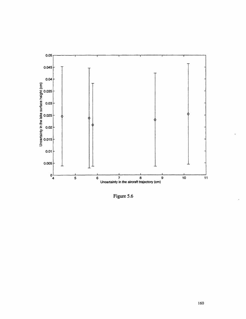
0.05 ----.,..------r-----.....------..----~---------

0.045

0.04

E~

E 0.0350>'Qi.s::.CD~ 0.03

'1::::senCD~ 0.025CO

-=.5: 0.02~c'lijt:~ 0.015c::J

0.01

0.005

I1

1110678 9Uncertainty in the aircraft trajectory (em)

5O'-----.--..------L-----...Io-...-------.I,.--------------~------'

4

Figure 5.6

160

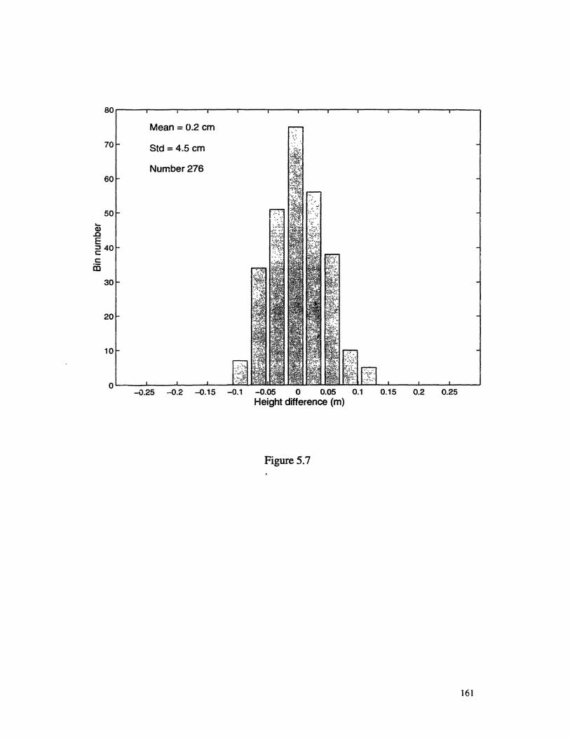
80 ..----..,...---~---,...----,----......-----.~--..----~--...,......------------

Mean =0.2 em

Number 276

Std = 4.5 em70

60

50~

Q)..cE~ 40c:iii

30

20

10

-0.25 -0.2 -0.15 -0.1 -0.05 0 0.05 0.1Height difference (m)

Figure 5.7

0.15 0.2 0.25

161

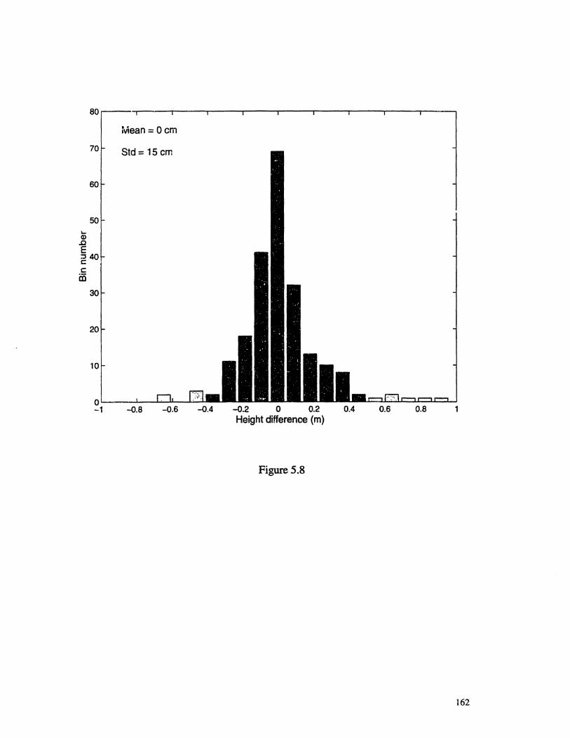
80 ...----....,.-----T"----r---__--~--_r_--_--_-_- __rviean =0 em

0.80.60.4-0.2 0 0.2Height difference (m)

-0.4-0.6

Std = 15 em

oI.....--.-----'---...I-:-~-......I~~.....

-1

10

50

20

70

30

60

s-a>..cE~40

c:iii

Figure 5.8

162

Chapter 6. Discussion and Conclusion

In this thesis, we have developed an algorithm for kinematic GPS surveying in high speed

vehicles, such as aircraft, based on Kalman filtering. Kalman filtering can use stochastic models

to update the estimates of position and velocity without a clear knowledge of their physical mod­

els a feature for kinematic GPS surveying. In kinematic mode, the velocity model is not as well

known as in the dynamic or quasi-dynamic mode, such as spacecraft positioning, whose processes

are governed by clear physical laws. The aircraft accelerates and decelerates fairly arbitrarily and

is hard to rnodel dynamically even in a short time span. In this situation, the application of sto­

chastic models such as random walks on velocities and positions of the aircraft can help us to uti­

lize the information from past observations to estimate the current state in a simple and straight­

forward way. In our application, Kalman filter also shows its ability to include estimation of aux­

iliary different parameters, such as temporal variations of the clocks and atmospheric delays in

GPS observations, together with the position changes of GPS receivers, all with appropriate sto­

chastic models. The use of a Kalman filter helps the kinematic algorithm to utilize continuous

temporal information of paraineters in the data analysis.

Without accurate ambiguity estimates, the carrier phase observations can not achieve cen­

timeter level accuracy_ Developing an ambigllity resolution technique suitable for kinematic GPS

measurements is the key point to use precise GPS carrier phase measurements at their full poten­

tial. The kinematic mode of aircraft GPS survey is more complicated and difficult than the static

mode or the ground kinematic mode, in which a measured spot can be re-occupied. The static C'r

repeated ground occupation of GPS receivers helps the determination of many model errors. The

ionospheric delay, multipath and atmospheric delay can be averaged out by long tilne observa­

tions. In kinematic mode, these benefits disappear. It is difficult to separate model errors, such as

uncorrected ambiguity bias from the motion of the GPS antenna. Thus we have to find a strategy

to determine the ambiguity from observation data in a short time span and to utilize all available

infonnation to solve the problems

In this thesis, we developed methods for reliably detennining integer L1 and L2 ambigu­

ities using dual-frequency carrier phases. The approach is taken in two different ways regarding

163

ofthe ambiguity problems both in initialization and non-initialization conditions. For initial ambi­

guity search, we used the widelane and extrawidelane combinations to obtain the position-free

initial guess for ambiguity sets~ The lane constraints (integer relationship) between the Ll/L2 dual

frequency phase measurements are used for the reduction of the ambiguity search space. We also

developed a new validation method which considers not only the RMS scatters of the phase resid­

uals and the changes of this scatter, but also the balance between the use of low elevation observa­

tions to improve geometry and the errors that may be introduced because of propagation medium

and multipath. For ambiguity changes dwing a flight, a method is developed to detect and fix the

cycle slips and to resolve the ambiguity for new satellites much faster for the initial search. The

method utilizes the available position infonnation to reduce the effects of the position, iono­

spheric and other errors on the ambiguity estimation. Also a pre-filter examining of the widelane

and extrawidelane can help us avoid the impact ofambiguity in the continuous estimation ofposi­

tion. The method we developed is flexible for different observation situation, and is capable of

solving the ambiguity for a moving object in a short time of period. The goal of our ambiguity

search method is not the reduction of computation time which most current methods on, but a

flexible, quick (shorter time span) and unique resolution regardless of experimental conditions.

To process the GPS data sets involved in kinematic GPS measurements, we developed a

robust software package to implement the algorithm based on the Kalman filtering and differen­

tial GPS technique. Our software takes the precise satellite orbit and clock information. By auto­

examining of data and ambiguity, it makes it easier for users to process the kinematic GPS data.

The use of this software is not limited to airborne laser altimetry but can also be used for many

types ofGPS kinematic surveying.

In the application of our software to the Long Valley mission, the repeatability of GPS

kinematic surveys has shown to be under 3 em by our runway tests and crossover analyses of the

laser data. The software handles the GPS data well for an aircraft flying at altitudes in the range of

1 to 10 km. In the tests with 1993 and 1995 GPS data in Long VaIle}' mission, our software

obtained good trajectories in all cases except for the case when there are problems in the original

data (such as the second trajectory part on Sept.. 14, 1993). The five take-off and landing tracks of

the aircraft trajectories matched within 3 em with an average of 1.8 ~m,

164

The application of GPS tracking into laser altimeter data analysis is also encouraging. The

measurement of elevation height over Lake Crowley shows a centimeter-lever statistical accuracy

in the repeat measurements. The profiles of the lake surface along the tracks are measured with

RMS scatter between 2.0 to 2.5 em. The differences of the profiles of the lake from different days

also agree within 2 em. Although the direct crossover analysis show a 4.5 cm point-ta-point scat­

ter, the near zero mean difference indicates such scatter can be smoothed out by repeat measure­

ments. The crossover analysis for Benton Crossing also shows good terrain ground measurements

with an average crossover residual under 1 em for 216 points even though the scatter is larger (15

em) due to rough local topography. The accuracy of the airborne laser altimetry can be assessed

from the statistical analysis of data collected. A more stable and reliable GPS trajectory can pro­

vide more qualified interpolation points for the laser measurements and a better statistical resolu­

tion can be then deduced for ground profiling.

The noise analysis in the flights over Lake Crowley indicates most errors of the current

altimetric data process are not directly related to those of GPS trajectories. Even when the formal

errors of GPS trajectory change from 4 cm to 10 cm because ofthe decrease ofthe observable sat­

ellites, the mean RMS of the estimated lake surface does not change significantly. Also the varia­

tions of the differences between the tracks over Lake Crowley have much higher frequency noise

than the static GPS. The autocorrelation length is 5 m (0.05 second under velocity of 100 m/s) for

altimetric measurements comparing to 70 second for GPS measurements. Those facts imply that

with a robust GPS algorithm., the errors of the estimated GPS trajectories are not the main sources

for the airborne altimetry. The long autocorrelation length of GPS measurements indicates it is

better to repeat the survey over the same area after a few minutes to smooth out the potential GPS

bias for a track over a few kilometers such as that over Lake Crowley (5km). In most tests here,

the estimated lake surface shape over the Lake Crowley shows that the differences between the

repeat flights are less than 2 em in most spots. It implies that the use of 5 em for the phase noise is

too large for the true behavior of GPS receiver. When a smaller noise level such as 0.5 em is used,

the single epoch uncertainties of the GPS trajectory will decease to 1 to 4 em.

Although GPS trajectory detennination has shown em-level accuracy here, there is still

165

room for improvements for the future airborne surveys. The post-fit residuals are slightly larger in

high altitude flights, especially for low elevation observations. For the flights at altitudes over 5

kID, there are possible unrnodeled errors arising from the atmospheric mapping function and iono­

spheric effects. With a thinner atmospheric path, the em vature of the ray is smaller than for a ray

that reaches the ground. Although we have used several mapping functions that have the ability to

model the height variation of the GPS receiver [Davis et aI., 990; Herring, 1992; Neill 1996],

none of these models has been tested at 5 to 10 km ellipsoidal height. Also the effects of phase

center rotation ofGPS receiver at high speed is still unknown. Ridgway et ale [1997] conducted an

antenna rotation test in the 1993 mission and found only 5 mm changes in the position. However,

the rotation under high velocity IDay be different. The GPS antenna 011 the roof of the T39 aircraft

is custom-designed and we do not have enough information for further antenna rotation test. Cur­

rent calibration flight tests are performed on the nearly straight trajectory sections of flight; thus

the effect of antenna phase may not been revealed in the repeat flights. Another concern related to

the repeatability of the GPS measurements is the position accuracy of the GPS base station. In a

50-100 km baseline, the vertical variation of the base station position transfers almost exclusively

into the measured heights ofthe aircraft trajectories (For a 20 em change in the vertical position of

the base station, the position of an aircraft 50 km away changed by 20 em and 0.16 cm in vertical

and horizontal directions, respectively.) The nearest pennanent GPS station at Casa Diablo is not

a good reference station for our reference station at Bishop because of the large and irregular geo­

detic displacements detected in Casa Diablo. So there is a need to measure the position of the

Bishop base station related to several other global GPS stations in the future airborne laser mea­

surements in Long Valley. By conducting long time static GPS measurements, we can also inves­

tigate the multipath and other location related errors around the base station.

Although there is no direct evidence that the changing satellite geometry increases the

variations of trajectories in the Long Valley experiments, the fonnal error of the aircraft vertical

position in a single epoch increase by a factor of two when the number of observable satellites

decreases from six to 4. When the atmospheric zenith delay is estimated, the situation worsens

(Figure 4.6). The atmospheric zenith correction affects the height determinations of the aircraft

directly and may be needed when the atmosphere change is strong. Thus in the design of flight

tracks, it is better to keep at least 5 satellites visible for the GPS measurements in the targeting

]66

segment of the flights.

The airborne laser altimeter system is potentially capable ofmeasuring changes of the ver­

tical displacenlents of the topographic surface with centimeter accuracy. However, the precise air­

borne laser altimeter measurement is a complicated technique involving a laser altimeter, an

inertial navigation system (INS), and GPS positioning for the aircraft. To achieve centimeter level

positioning, the GPS trajectory determination of the airplane is a key element. With a fast resolu­

tion algorithm and a high quality centimeter-level GPS trajectory, it is possible that the airborne

laser altimeter technique could facilitate rapid, direcl and precise surface deformation monitoring

in near real-time, which should benefit the study of many geodetic events such as volcanic erup­

tions. After several years of repeat flights, we expect the airborne laser system could reveal the

vertical uplift in the top of resurgent dome near Long Valley caldera, which is expected to reach 4

em/year. The GLAS launch is already planned for 2001. We hope the algorithm and software

developed here could provide some useful experience for the future GPS tracking application in

tile centimeter space laser altimetry.

167

168

Appendix A: Atmospheric Delay Modeling

The atmospheric delay contribution to the delay of the GPS signal in given by

La = Jn(s)ds- JdsaIm vac

(A-I)

where n(s) is the refractive index along the ray path. The fIrst integral in (A-I) is along the real

path in atmosphere and the second integral is along the vacuum path of the ray. Since the values

of n(s) are not well-known, the equation (A-I) is approximated by the introduction of zenith

delay, the atmospheric delay determined in the zenith direction, and a "mapping function" which

is the ratio of La in any directions to the zenith delay. Azimuth asymmetric effects exist [Chen

and Herring, 1997] but, to simplify the problem, most of atmospheric delay models still use a

common symmetric assumption in the mapping functions. We re-write the atmospheric delay

equation (A-I) as

(A-2)

where Zd1 Zw are the hydrostatic (dry) and wet components in the zenith directions; md(E) and

mw(E) are the dry and wet mapping functions; f: is the elevation angle of the ray. Our kinematic

GPS software has options to allow the user to choose several different atmospheric models. We

discuss them in the following sectionw

Saastamoinen Zenith Delay

The most popular fonnula used for zenith delay is that developed by Saastamoinen

[1972]. It relates the pressure, temperature, and humidity as well as the latitude and height of the

site to the propagation delay in the zenith direction. The dry zenith delay Zd is defined as:

O.002277PoZd = J{cp,H) (A-3)

where Po is the total pressure in mbars of tile point, uf(<fl, H) is a function which accounts for the

variations of gravity with the latitude ~ and altitude H (in kIn) of the point, and is given in [Davis,

169

1985]

f(~,H) = 1-0.0026(l-2sin 2~)-0.00031H (A-4)

The "wet" zenith delay Zl~ is defined related to wet pressure eo (in mbars) as

_ O.002277eo(1255 )Zw - f( <p, H)- r; + 0.05

where To is the absolute temperature of point (in Kelvins).

(A-5)

The use of mapping function has several choices: Marini model, CfA-2.2 model, MIT

Inodel (both temperature and seasonal temperature), and tile Niell's HMF model [1996].

Marini model

The Marini formula is written as [~1arini, 1974]

1m(£) =. A/(A + B)

SIDE + ---------­sine + 0.015

(A-6)

where A is the Saastamoinen zenith delay given by sum of (A-3) and (A-5) and B is given by

-3B= 2.;~x; exp(-O.14372H)cp, )

Equation (A-6) is used for both dry and 'wet mapping function.

efA model

(A-?)

After it was found that Marini formula was inadequate for the lower elevation of observa­

tions especially those below 150, Davis (1986) developed a model known as CfA-2.2:

170

m(E) = ----------. a

SInE + bsinE + -.--0-0-0-9

SInE - .

With

a = 0.001185[1 + 0.6071xlO-4(Po-1000)]-3 -2

-O.1471xIO eo+O.3072xIO (To-20)

+ O.l965xlO-1W + 6.5)

-2-O.5645xIO (h t -II.231)

b = 0.001144[1 + 0.1l64xlO-4(Po-1000)]-3 -2+ O.2795x10 eo + 0.310910 (To - 20)

+ 0.3038x10-I (P + 6.5)

-1-O.1217xIO (h t -ll.231)

(A-8)

(A-9)

where Po is the total pressure (mbars), eo is the partial pressure ofwater vapor (wet) (mbars), To is

the temperature (in Celsius), Pis the tropospheric temperature lapse rate (K km- I ) and ht is the

height of tropopause (in km).

MTTmodel

The efA mapping function strictly requires the knowledge of the upper atmospheric con­

ditions whiell are not available for most locations. Herring (1992) developed a mapping function

that depends only on the surface temperature Ts' latitude cp and ellipsoid height ofpoint Hs:

m(E) = 1+ a/(l + b/(l + e)). a

smE+ . bSffiE+-.-­

SinE + C

With coefficients G, b, c in dry mapping function as

(A-lO)

171

a = [1.232 + 0.013 coscp - O.0209Hs

+ 0.00215(Ts - 10)]xlO-3

b = [3.1612-0.013 cosq> - O.0331Hs

+ 0.00206(Ts - 1O)]xlO-3

c = [71.244-4.293coscp-O.149Hs

-0.0021 (Ts - 10)]x10-3

and coefficients a, b, c in wet mapping function as

a = 0.583-0.011 cos<p - O.052Hs

+ 0.0021:(Ts -10) ]x10-3

b = [1.402+0.102coscp-O.lOlHs

+ 0.0020(Ts - 10)]xIO-3

c = [45.85-1.91 cos<p-l.29Hs

+ 0.OI5(Ts -IO»)xlO-3

HMFmodel

(A-II)

(A-12)

Arthur Niell [1996] developed expressions for mapping function (NMF function). The for­

mula of NMF mapping function is as same as that of MIT function except the coefficients. The

coefficients of NMF mapping function depend on the latitude and height above the sea level of

the observation point and the day of the year. For details of coefficient table of NMF, refer to

Niell [1996].

172

Reference

Chen, G. and T. A. Herring, Effects of atmospheric azimuth asymmetry on the analysis of space

geodetic data, 1. Geophys. Res. 102, 20,489-20,502, 1997

Davis, J,L., Atmospheric propagation effects on radio Interferometry, Ph. D. Thesis, MIT, Cam­

bridge, MA, 1986

Marini, J. W. and Murray, C. W., Correction of laser range tracking data for atmospheric refrac­

tion at elevations above 10 degrees, NASA report X-591-73-351, Goddard ~pace Flight

Center, 1973.

Herring, T. A., modeling atmospheric delays in the analysis of space geodetic data, in Refraction

of trans-atmospheric Signals in Geodesy, eds. J. C. Munck and T. A. Spoelstra, Nether­

lands Geodetic Commission Publications in Geodesy, 36,157- 36,164, 1992.

Saastamoinen, Contribution to the theory of atmospheric refraction. Bulletin Geodesique, 107,

13-34, 1972

Niell, A. E., Global mapping functions for the atmosphere delay at radio wavelengths, J. ~;'Zo­

phys. Res., 101, B2, 3227-3246, 1996.

173