1

Abstract—This paper provides a wide perspective of the

potential applicability of Graphical Processing Units (GPUs)

computing power in robotics, specifically in the well known

problem of 2D robotic mapping. There are three possible ways of

exploiting these massively parallel devices: I) parallelizing

existing algorithms, II) integrating already existing parallelized

general purpose software, and III) making use of its high

computational capabilities in the inception of new algorithms.

This paper presents examples for all of them: parallelizing a

popular implementation of the grid mapping algorithm, using a

GPU open source linear sparse system solver to address the

problem of linear least squares graph minimization and

developing a novel method that can be efficiently parallelized and

executed in a GPU for handling overlapping grid maps in a

mapping with local maps algorithm. Large speedups are shown in

experiments, highlighting the importance that this technology

could have in robotic software development in the near future, as

it is already doing in many other areas.

Index Terms— Mobile Robots, Robot Programming,

Graphical Processing Units, Robotic Mapping.

I. INTRODUCTION

lthough microprocessor manufacturing technology is

continuously improving, it is reaching the point in which

physical limits are becoming a major concern. Memory speed

and power have imposed walls for increasing processing

performance by scaling the clock frequency. Over the last

years, Moore’s law and performance improvements have been

maintained mainly due to one reason: multi-core processors

(multiprocessors). In multiprocessors, several CPU cores are

packaged into a single chip, taking advantage of their

proximity, for example when accessing the cache memory.

Some well known examples are Intel Dual-Core and Quad

systems, Sony Cell (8-core) processor inside PlayStation3 and

the PowerPC Xenon (3-core) processor in Microsoft’s Xbox

360.

Together with multiprocessors, new programming models

have emerged in order to manage and exploit the available

Manuscript submitted October 8, 2010. This work was supported in part

by the Spanish R&D National Program ( Robonauta project. Ref: DPI2007-

66848-C02-01)

Authors are with the Center of Automation and Robotics (UPM-CSIC), C/

Jose Gutierrez Abascal, 2, 28006, Madrid (phone: +34-656274654 fax: +34

91 366 77 29 e-mail: diego.rlosada@upm.es)

parallelism of those systems. Single processors can implicitly

implement in hardware some degree of parallelization

pipelining instructions, but when dealing with multiprocessor

architectures parallelization must be explicitly implemented by

the programmer. Message Passing Interface (MPI) is the de

facto standard for high performance distributed computing,

while OpenMP is probably the most extended solution for

multiprocessing in shared memory systems, as multi-core

CPUs.

Manufacturers of graphical processing units have been also

continuously improving their systems, leading to multi-core

Graphical Processing Units (GPUs) where each core contains

also a large number of Arithmetic and Logical Units (ALUs)

specialized in parallel processing of graphics as textures,

visibility, image processing, etc. Also the large market for

graphics cards with ubiquitous 3D graphics (games, CAD,

multimedia, etc), has lowered the cost of very powerful

devices that can fit into the class of what is known as

commodity hardware. Major GPU manufacturers have recently

released tools and programming models that allow

programmers to access such computing power: ATI (now part

of AMD) development platform is called ATI Stream, and the

NVIDIA development system is called Computed Unified

Device Architecture (CUDA).

The CUDA approach has gained large attention and many

researchers have found it a powerful platform for boosting

their computations. Furthermore, several libraries as CUBlas

(a port of the Basic Linear Algebra Set – Blas) or GpuCV

(largely compatible with OpenCV) for computer vision have

been developed that let researchers take advantage of the

computing power of GPUs without requiring explicit

parallelization of algorithms. Applications such as Matlab or

GIMP have also been provided with CUDA extensions that let

the applications transparently benefit from GPUs processing.

It is our belief that the robotics community should also

benefit from adopting and using such technology. To this

avail, three main lines could be followed:

Parallelize and port existing algorithms to execute in

GPUs

Take advantage of already developed general purpose

math or computer vision libraries and tools

Develop new algorithms explicitly taking into account

the computational capabilities of such devices

Many algorithms in mobile robotics are computationally

GPU-Mapping: Robotic Map Building with

Graphical Multiprocessors

Diego Rodriguez-Losada, Pablo San Segundo, Miguel Hernando,

Paloma de la Puente, Alberto Valero

A

2

intensive. Amongst them, the map building or Simultaneous

Localization and Mapping - SLAM problem [1], [2] has

gained great attention in the last decades, with a prototypical

case study of indoor wheeled mobile robots equipped with

laser rangefinders.

Section II presents current related work on GPU robotic

applications; note that most contributions are related to the

computer vision domain. This paper presents a demonstration

of GPU computing applied to the SLAM problem in the three

lines stated above, showing also its high potential applicability

in domains other than vision. Section III shows how a publicly

available implementation of the grid mapping algorithm can be

parallelized over a GPU to obtain high computational savings.

Section IV uses a general GPU optimized sparse linear system

solver to address the graph SLAM problem defined as a least

squares minimization over a graph of poses. Section V

implements a novel algorithm for handling overlapping

between different grid maps, which can be efficiently applied

thanks to the computing power of GPU. Section VI reports on

simulated and real experiments combining some of the

previous techniques. A discussion on related issues is

presented in section VII and finally, conclusions are

summarized in section VIII.

II. GPU COMPUTING IN ROBOTICS

A. Related work

In recent years there has been an upsurge of interest in GPU

computing applied to robotics. Some applications address

topics such as grasping with manipulators, solving the

algebraic and geometric problem with GPUs [3]. However,

most of the related literature is actually found in the computer

vision domain, as in the early work of Michel et al. [4] which

tracked 3D objects with cameras using the GPU to achieve real

time performance when controlling a humanoid. Other works,

such as [5] try to speed up the typical processing and matching

of SIFT features among different frames for localization

purposes, while more complete multimodal perception

approaches as [6] includes Bayesian solutions with particle

filters. There exist research groups and projects fully devoted

to this area, as the gpu4vision project [7].

In the mapping with laser rangefinders domain, the work of

Yguel et al. in 2007 [8], addressed the problem of updating a

2D probability grid with a novel formulation of the required

polar to cartesian grid conversion which takes into account the

actual beam model. A more recent work is found inside the

well known Slam6D open source project [9], where NVIDIA

CUDA is used for speeding up the 3D point clouds registration

and ICP matching [10].

It is important to highlight the merits of [4] [8], since current

general purpose CUDA tools were not available at the time, so

programmers had to deal with specific graphics APIs.

Nowadays, these tools allow much more simple development,

and even robotic specific software frameworks include support

for such tools as, for example, ROS [11] does with CUDA.

B. Overview of nVidia CUDA architecture

CUDA exposes the NVIDIA multi-core GPUs computing

capabilities through the following elements (Fig. 1):

Thread hierarchy. The execution unit in CUDA is a

kernel, which is structured in a so called grid (a 1D or 2D

array) of blocks, each block in turn arranged in another (up

to 3D) array of threads. Unlike CPU multithreading, every

thread of the same kernel has to run exactly the same code,

so typically a kernel is used to perform the same task

concurrently over a large set of data. Built-in variables are

used in the thread code to access its indices in the block as

well as the block indices in the grid. These indices are

typically used in the thread code to address the particular

chunk of data that the thread must handle.

Memory hierarchy. Each thread has its own private

memory space and registers, each block has a shared

memory that can be accessed by all threads in the block,

and there exists a global memory accessible by all threads.

The system is completed with two read-only memory

spaces: the constant memory and the texture memory. The

shared memory is built inside the GPU, so it is faster than

the global memory that is outside the GPU (but located in

the device, i.e. the graphics card).

Thread synchronization. All threads in a block can be

forced to wait at a given point until it is reached by the

remaining threads.

Fig. 1. CUDA architecture

The CUDA architecture is available to the programmer via

some extensions of the C language as well as a runtime library.

With these extensions the programmer can define kernels,

declare the type of device memory required for each data, and

synchronize threads.

A typical working cycle consists of the following steps:

allocating memory on the device (graphics card), copying data

from host (PC) memory to the device, launching one or several

kernels, and finally copying the results from device to host

memory.

To achieve a good overall performance several things have

to be considered. The threads are managed by hardware, so

they have practically no execution, changing, switching or

finishing overheads. The GPU bottleneck is typically memory

access, relatively slow compared to processing. Fortunately,

the memory latency can be typically hidden if there are enough

threads to be scheduled for execution. In practice this implies

that a kernel must launch thousands of threads and that an

adequate selection and usage of the different memory types of

Kernel Grid

Block Block Block

Device Memory

Local (thread)

Shared (block)

Constant

Global

Block Block

fast (registers)

Threads

fast (cache-like)

slow

fast (read only)

3

the GPU is critical to achieve adequate speedups.

III. GRID MAPPING

Probabilistic grid maps [12] divide the environment into

small square cells and compute the probability of occupancy

for each cell, given the sensor measurements and assuming that

the correct robot poses are known. The probability of the map

m given all the data (both poses and observations) ts up to

time step t , can be factorized into the probability of each

cellcm as follows:

| |t t

c

c

p m s p m s (1)

As derived in [13], the probability of each cell can be

computed recursively as:

11

1

( | )

(1 )( | ) ( | )1 1

(1 ( | )) (1 ( | ))

t

c

tpriorc c t

t

c c t prior

p m s

pp m s p m s

p m s p m s p

(2)

where priorp denotes the prior probability of occupation

which is assumed to be equal for all cells, (an initial parameter

of the algorithm), and ( | )c tp m s is the probability of a cell

occupancy conditioned only on the observation ts at a certain

time step t , as defined by the probabilistic sensor model.

Irrespectively of the sensor model, (1) and (2) show that

updating the probability in each cell can be performed

independently; this is a cornerstone for a straightforward

massive parallelization. The work presented in this paper takes

a very well known publicly available implementation in

CARMEN [14], and implements it for efficient GPU

computation by finding and adequate parallelization.

Fig. 2. Bresenham ray trace of one beam from a laser scan reading

The CARMEN grid mapping algorithm traces a line

segment for every beam of each laser scan (typically 180 laser

beams spaced at 1º intervals), and iterates using the

Bresenham algorithm [15] as shown in Fig. 2. At each step the

update procedure requires a nested for loop, summarized in

Fig. 3: the outer loop iterates over the different beams, and the

inner one over the cells crossed by the ray, which are updated

according to (2).

The proposed parallelization unfolds the nested for loop in a

CUDA kernel, with one block per laser beam (outer loop), and

each block made up of a vector of threads, one for each cell

that has to be updated (inner loop). Since the number of cells

differs for each ray in the general case, each block would

require a variable number of threads depending on the actual

measurement. CUDA, however, only allows a fixed number of

threads per block. Although this number depends on the

hardware platform, its minimum size is 256 threads, which can

accommodate a sensor range of 6.4 meters for a cell size of 2,5

cm and 12,8 m for a cell size of 5 cm, which are reasonable

values for real applications. The proposed kernel will be

typically composed of 360 blocks, each one with 256 threads,

i.e. a total of 92160 threads for handling each laser scan.

The first step is to allocate and copy the input data from

host memory to the GPU device memory. In this case it is

necessary to copy the whole laser datats (including all

measurements from all time steps, as well as the robot poses),

the initial probability grid 1( | )tp m s , and the input

parameters. Next, a kernel is launched for every time step to

process the corresponding scan ts . Finally, the resulting

updated probability grid ( | )tp m s is transferred back to the

host memory.

1Function ( ( | ), )

foreach

foreach

( | ) (Eq. 2)

endfor

endfor

t

t

t

t

c

Updt p m s s

ray s

c ray

p m s

1( | ), / /GPU Memory

Kernel(360,256, )

//360x256 GPU threads

(Block ,Thread )

= ( , )

( | ) (Eq. 2)

t

t

t

c

p m s s

UpdtThread

UpdtThread i j

c ComputeCell i j

p m s

Fig. 3. Grid mapping CPU sequential algorithm structure (left) vs. GPU

parallelized version (right). Note that this is just the update of a single scan,

and must be done for each measurement.

Two real different datasets named Fr079 and Fr101 with the

robot poses already corrected (see Acknowledgment, more

details in [16]) have been used for the experiments and

processed with different CPU and GPU configurations. The

results are summarized in Table I. In the CPU, a slightly

modified version (as using the same floating point data types

in order to achieve a fair comparison) of the CARMEN

algorithm is used, while the GPUs run our parallelized (but

algorithmically identical) version. In both cases, all input data

is loaded into memory before starting the computation to

eliminate delays resulting from reading data from a hard drive.

While laptop GPUs can double the speed of a CPU, powerful

graphics cards as the GTX280 show improvements in speed up

to 58X. TABLE I PROCESSING TIMES IN SECONDS AND EFFICIENCY

DATASET

PROCESSOR Fr079 Fr101

2Ghz Core 2 Duo T7250 11,5 (1) 25,3 (1)

3,2Ghz Pentium D 15,2 (0,76) 30,9 (0,82)

GF 8400M GS (laptop) 6,26 (0,92) 12,17 (1,04)

GTX 280 (desktop) 0,26 (1,47) 0,52 (1,62)

4

The evaluation of results in terms of efficiency could be a

controversial issue, since the comparison is done between two

radically different architectures. Table I presents the relative

efficiency of the GPU parallelization taking into account the

number of multiprocessors (control units, 2 in the GF8400 and

30 in the GTX280) and comparing with the Core2Duo. Super

linear efficiency is possible due to the specialized GPU

architecture which has a much higher number of arithmetic

units (CUDA cores, 16 in the GF8400 and 240 in the

GTX280). Obviously, using this latter number for computing

efficiency will produce very poor results. In any case, we

consider that absolute timings should be the critical factor to

be taken into account because they represent the ultimate

performance of the robot, irrespective of how well are the

algorithms parallelized or the GPU resources exploited.

For the GPUs, memory transfer times to and from the

graphics card have also been included in the results of Table I.

These delays are unavoidable, and must be included in the

absolute timings, just as transfer times from main memory are

included in the CPU timings. Memory transfers could play a

crucial role in the parallelization performance, though. Table

II summarizes data transfers involved in the computations with

the GTX280 card. First, the grid map, the parameters and the

whole data set are transferred from host to device. After all the

kernels have been launched (one per scan), the resulting grid

map is transferred back to the host memory. As can be derived

from the reported results, these times are low compared with

the total computing time. This is one of the reasons which

explain the good performance obtained by the GPU: just four

large memory transfers are carried out, and their delays are

amortized along a high amount of computation.

TABLE II. MEMORY TRANSFERS (3,2GHZ PENTD - GTX280)

Fr079 Fr101

Size of grid map (Mbytes) 5,63 16,64

Size of grid params (bytes) 52 52

Size of data (# scans - Mbytes) 3118 - 4,55 5299 - 7,74

Transfer grid host to device (s) 0,0046 0,012

Transfer params to device (s) 0,0018 0,0018

Transfer data host to device (s) 0,0035 0,0053

Transfer grid device to host (s) 0,0046 0,012

Especially relevant is the fact that every data transfer has a

time lower bound, for example, transferring just 52 bytes of

the parameters requires 1,8 milliseconds. Thus, performing

exactly the same computation but transferring at each time step

the resulting grid map from and to the GTX280, will require

28 seconds for the Fr079 dataset and 124 seconds for Fr101.

Similarly, transferring at each time step just the laser scan

acquired at that time step instead of the whole dataset at once

and without transferring the grid map, could require about 6

seconds for Fr079 and 10 seconds for the Fr101 datasets. It is

concluded that minimizing and grouping memory transfers is

extremely important to achieve good performance.

Fig. 4 shows the result from FR079 data set with a GTX280

GPU, visually identical to the one obtained with CPUs.

Fig. 4. Fr079 building map, computed in 0,26secs with a GTX 280 GPU

It is also important to analyze the effect of the appropriate

use of device memory. Table III shows the relative

performance of the GPU (GF8400M) with respect to the CPU

for three different memory usages. If all the data is stored in

the global memory of the device, the performance of the GPU

implementation is even worse than that of the CPU version.

However, moving a fraction of the data to shared memory (just

the Bresenham parameters of each ray), the computational

savings become clearly visible; note that only the first thread

of the block computes them while the remaining threads have

to wait. The use of constant memory that provide faster access

to common read-only parameters allows further savings.

TABLE III EFFECT OF GPU MEMORY USE

Device memory use Processing time of GPU

compared with CPU

All data in global memory, each thread

computing beam data 150%

Common block (beam) data in shared

memory, computed only by one thread 65%

Input parameters in read-only constant

memory 50%

It should be highlighted that the CARMEN reference

algorithm is not necessarily the best nor the fastest one. The

contribution of this paper is the achieved relative improvement

in speed by an adequate GPU parallelization of a given

algorithm implementation. More details about the proposed

grid mapping CUDA parallelization can be found in [17] as

well as in the source code available at [18].

IV. GRAPH OPTIMIZATION

A common approach to the SLAM problem dates back to

Lu and Milios [19], where a network of relations between

robot poses is constructed and the Maximum Likelihood (ML)

map is computed by brute force least squares minimization

over the graph. Since then, a lot of research in SLAM has used

some kind of error minimization over a graph of relative

spatial constraints between poses (see section III of [20] for

related work).

The map of the environment can be represented by a

weighted graph ( , )G V E where the set of vertices V are

the robot poses (that can also be represented for convenience

as the state vector x ), and the edges E are defined by the

constraint equations ( )f x between those poses with expected

5

values u and variances , typically extracted from odometry

and feature correspondences. Finding the most likely map can

be achieved by solving a linear problem of the form Ax b .

The probability of the state can be written as:

1( ) exp ( ) ( )T

P x f x u f x u (3)

If ()f is linearized around value F with Jacobian J as

F J x and the residual r is defined as u F , the

negative log likelihood to be minimized is of the form:

1log ( )T

P x J x r J x r (4)

To minimize this cost function, we can differentiate with

respect to x and set to zero, resulting in:

1 1T TJ J x J r (5)

This equation is equivalent to an Extended Information Filter,

where 1TA J J is the information matrix. When this

system is solved iteratively recomputing the Jacobian at each

step, the method of nonlinear least squares is obtained.

Solving (5) as a dense system on the CPU has been done in

the past only for reference purposes because of its practical

intractability, but the nature of the SLAM problem actually

makes this system sparse, due precisely to the sparse structure

of the underlying graph. Although a lot of improvements have

been done in graph based SLAM, the efficient solution to this

sparse system remains of high interest, as shown in a very

recent work by Grisetti et al. [21], where the system is solved

using a sparse solver package named CSparse.

We consider here the possibility of solving (5) with the CPU

sparse solver SuperLU [22], and compare the result with a

GPU similar counterpart: Concurrent Number Cruncher, CNC

[23]. CNC is a CUDA optimized sparse solver that provides a

high level software interface which allows the programmer to

integrate it in another application without needing to know

about parallelization or internal CUDA usage. Thus, the

implementation in both cases is straightforward: the

information matrix and vector of (5) are computed, and passed

as parameters to either SuperLU or CNC solvers.

This experiment uses the synthetic data of a typical city

orthogonal environment, found in OpenSLAM [24] TORO

[20] package, defined by a graph of 10000 nodes (poses) and

64311 edges (constraints), which can be simplified or

replicated to create environments with 4,1k, 20k, 30k and 40k

nodes. The initial estimation for poses is obtained with a

spanning tree instead of the initial values for both CPU and

GPU solutions, in order to avoid excessive linearization errors

as pointed out in the Sparse Pose Adjustment algorithm [25].

Fig. 5 shows the initial graph, prior to the tree initialization

and the graph optimization, as well as the final graph, which

minimization has been computed with CNC in a GTX280

GPU.

Fig. 5. Minimization of a graph of constraints between poses, before (left),

and after (right) the minimization, computed with a GTX280 in 0,65 secs.

Table III shows the comparative performance of both

algorithms for a single iteration of the sparse solvers. In both

cases the same computer is used. It should be noted in advance

that an absolutely fair comparison is simply not possible for a

number of reasons: SuperLU uses double precision, while

CNC can only use float, an issue that is known to hinder

numerical convergence. Moreover, SuperLU is exact, while

CNC is iterative.

TABLE III PROCESSING TIME (SECONDS) OF GRAPH MINIMIZATION

ENVIRONMENT

(POSES, CONSTRAINTS)

PENTD 3,2GZ

SUPERLU

PENTD 3,2GZ + GTX280

CNC

4125, 5541 0,37 0,65

10k, 64k 3,39 3,71

20k, 138k 9,78 8,03

30k, 212k 20,4 11,8

40k, 286k 40,2 17,2

The computational gains are not as impressive as in the

previous section, and only get visible as the environment size

increases, with CNC reaching more than a 2X speed up

compared with SuperLU. CNC, set to run a maximum of 1000

iterations with a final error threshold of 2.5e-4, also achieves a

slightly better error reduction.

In this case reported results are not as impressive as in the

previous section, possibly due to the iterative structure of CNC

where each iteration driven by the CPU invokes many kernels

to compute basic sparse matrix operations in the GPU. It

becomes very difficult to compete against an optimized exact

solver even for a powerful GPU.

In any case, the interesting point here is that an available

software package has been used without any concern about

parallelization, and our algorithm has doubled its speed just by

plugging such software while releasing CPU time that could be

used for other purposes. Note however that this advantage

could become useless with high end CPUs as Core i7 running

tuned exact solvers, and this could be an important field of

further study (as reported in section VIII).

V. GRID MATCHING

In SLAM, the data association procedure tries to find

correspondences between different data sets. In many SLAM

algorithms, the space is subdivided by different means in order

to deal with the computational complexity as well as to

minimize inconsistency issues. Both in this kind of approaches

and in graph based SLAM, it is common to attach to the nodes

some local representation of the environment (named local

6

maps or submaps). In order to detect loop closures and

introduce new constraints or information, it is necessary to

compare two submaps. This section presents a novel approach

that takes advantage of the GPU in order to minimize the error

of two overlapping submaps, not only searching for

correspondences but also dealing with physically unfeasible

configurations. The presented approach is a simple local

solution, but as will be shown, it opens new possibilities in the

correspondence search problem thanks to the GPU computing

power.

Let us now consider two overlapping grid maps ,A bM M

with a relative initial pose ( , , )T

AB x y r . Fig 6 shows an

example in which the maps correspond to a corridor. White

areas are free space, black areas correspond to obstacles or

walls and blue areas are unknown or unexplored. Under the

static world assumption, it is clear that such spatial

configuration is not physically possible, as some clearly

occupied cells in map B fall on previously labeled as free

space in map A.

Fig. 6. Overlapping grid maps in an initial physically unfeasible

configuration. Map B is drawn translucent for clarity.

We can try to define a cost function that measures the

discrepancy of two overlapping grid maps by summing up all

the differences of individual overlapping cells. For such

purpose, a mapping between the cell indices Bc of a given cell

in map B and the corresponding indices Ac in map A has to be

defined. If M is a function that converts from cell indices to

real coordinates, taking into account the cell resolution and the

map reference frame offset with respect to the origin of

indices, the following relation can be established:

1 T( )A A AB B B c r c (6)

where T( )AB r is a compact representation of the change of

base between both reference systems. Now, an error function

can be defined as:

( , , ) ( ) ( )A B

B B

A B AB A B

M

e M M p m p m

c c

c

r (7)

The problem is that the cost function (7) is typically not

smooth, thus it is not suitable for common gradient based

minimization techniques. If we represent the cost value for

different initial ABr positions for the example depicted in Fig.

6 we get the cost function represented in Fig. 7. It is easy to

see that an initial position close to a sharp edge would take the

solution quite far from the initial position following the

gradient direction. While there might exist a very close

solution just a step aside, it would be difficult to reach due to

the zero gradient.

-12

-10

-8

-6

-4

-2

0

24681012

0

0,01

0,02

0,03

0,04

0,05

0,06

0,07

-9 -8 -7 -6 -5 -4 -3 -2 -1 0 1 2 3 4 5 6 7 8 9

X d

isp

lace

men

t (m

)

Co

st (

err

or)

Y displacement (m) Fig. 7. Cost function for equation (7) and the parallel corridors submaps

example. The central valley corresponds to the matching case, and the flat

areas in the sides represent non overlapping configurations. Note the

symmetry along the X axis due to the symmetry of the environment.

This problem cannot be avoided by directly smoothing the

cost function, as that would obviously be very computationally

expensive. Instead, a natural smoothing can be induced in the

cost function by avoiding sharpness in the submaps by simply

blurring them, propagating dark areas onto white ones, which

is a simple operation that needs to be done just once.

Fig. 8. Blurring a submap to smooth the resulting cost function

The large flat areas with zero error that correspond to non

overlapping configurations are another problem, as any

minimization procedure performing a large step (separating the

submaps enough) would arrive at such a non informative

minimum. To take into account the fact that the desired

solution is the closest to the initial position 0

ABr , a weighted

term can be added to (7), resulting in:

0

0

( , , , )

( , , )

A B AB AB

A B AB AB AB

h M M

e M M K

r r

r r r (8)

where 2 2 2 2

AB x y L r is the weighted Euclidean

norm that uses L to normalize angular into distance units. With

these modifications, the cost function depicted in Fig. 7

becomes more adequate for minimization purposes, as shown

in Fig. 9.

ABr

BM

AM

7

-12-8

-404812

0

0,02

0,04

0,06

0,08

0,1

0,12

0,14

0,16

0,18

-12 -11 -10 -9 -8 -7 -6 -5 -4 -3 -2 -1 0 1 2 3 4 5 6 7 8 9 10 11 12

X d

isp

lace

men

t (m

)

Co

st (

err

or)

Y displacement (m) Fig. 9. Final cost function with (8) and submaps blurring

Once the cost function is defined and can be evaluated using

(8) for every possible relative pose, the Broyden–Fletcher–

Goldfarb–Shanno (BFGS) algorithm, which is well known to

perform well in many situations, is applied. At each iteration,

the value of the cost function and its gradient are computed

according to the four point formula and, afterwards, they are

fed to the open source implementation of [26].

To analyze the performance of the algorithm in terms of

accuracy, the following experiment was conducted with two

grid maps corresponding to the same corridor. As shown in

Fig. 10 there are different physical feasible configurations or

solutions depending on the initial pose: if the initial pose is

close to the center, then the most likely solution is that both

corridors are the same, but if the initial position is not so close

to the center, then it could be more likely that the corridors are

actually parallel.

Fig. 10. The minimization leads to different configurations depending on the

initial pose: case A) the two submaps correspond to the same corridor (top),

and case B) (bottom), the submaps correspond to parallel corridors. The cyan

ellipse represents the information (proportional to the Hessian)

The results in terms of accuracy are summarized in Table

IV, where different initial pose intervals are used. The first two

lines correspond to the matching case A, and the last one to the

parallel corridors case B. The experiment is repeated with one

hundred random initial poses for each setting. It can be seen

that for case A, a very high percentage of accurate or very

accurate solutions is reached, while in the second case B the

accuracy seems lower. Only the Y and final values are

checked, as the nature of the environment does not provide any

information in X.

TABLE IV ACCURACY (M, RAD)

ACCURACY (M, RAD)

CASE, NOISE (M,RAD) |y|<0.025

|θ|<0.045

|y|<0.05

|θ|<0.09

|y|<0.2

| θ |<0.16

A x,y,θ ±0.5 99% 100% -

A x,y±1.5, θ±0.38 98% 98% 98%

B x±1.5 y5±1.5 θ±0.38 62% 73% 93%

It is important to highlight that inaccurate solutions are not

necessarily incorrect, although they present a poorer final

alignment between the corridors. In any case, the algorithm

still outputs a physically feasible configuration that is more

likely than the initial one, as can be seen in Fig. 11.

Fig. 11. An example of poor final alignment, but providing a physically

feasible position.

The main contribution of this section is not only the novel

minimization method proposed, but also its potential

applicability to online mapping problems thanks to GPU

computing, which was taken into account while designing this

algorithm. Most of the processing time consumed by the CPU

is taken by Eq. (7), which is a large summation over all the

cells of a grid map and has to be repeated every time the cost

needs to be evaluated. This summation can be parallelized in a

CUDA kernel as shown in Fig. 12. The grid is composed by m

x n blocks, each one with 256 threads. The parallelization uses

a hierarchical summation scheme to avoid excessive waits due

to synchronization locks that appear in the last line of the

function SumThread, which must be necessarily performed as

atomic. If just one single variable were used as in the

sequential version, all the threads of every block would always

collide, as they are executed simultaneously. Consequently,

using the size of the blocks for the auxiliary array is a

reasonable option, although other sizes could even perform

better depending on the GPU capabilities. Moreover, the

CUDA atomicAdd() function only works with integers, so a

scaling factor S is needed (see the source code [18] for details

about this parallelization).

A) Matching (same corridor) case

B) Non matching (parallel corridors) case

8

= ( , , )

0 // as float

foreach

( , ) (Eq. 6)

( ) ( )

endfor

return

A B

A B AB

B B

A AB B

A c B c

error Error M M

s

M

f

s p m p m

s

r

c

c r c

256

0

= ( , , )

[256] 0 // integer values

Kernel( , 256, )

1 [ ]

(Block( , ), Thread( ))

= ( , , )

( , ) (Eq. 6)

[

A B AB

i

B

A AB B

error Error M M

s

m n SumThread

return s iS

SumThread i j k

ComputeCell i j k

f

s k

r

c

c r c

] ( ( ) ( ))A BA BS p m p m

c c

Fig. 12. CPU sequential implementation of Eq. (7) (left) vs. GPU parallelized

version (right).

The average number of L-BFGS iterations is 35, with an

average computation time for the whole minimization

procedure of 6.0 seconds (with a Core 2 Duo @ 2 Ghz), while

this time is reduced down to 0.15 if the same computation is

carried out with a GTX 280 GPU, i.e. a speed up of 40X is

achieved. The memory transfer overhead is negligible in this

case, as the local grid maps (which are small) need to be

transferred just once to the device, something that can be done

as soon as the submaps are available, typically long before the

matching procedure.

VI. EXPERIMENTS

To illustrate the applicability of the above described

techniques, both simulated and real data experiments have

been carried out. Input log files of laser scans and robot poses

were preprocessed: local grid maps of a limited fixed size are

built defining new nodes which are sequentially connected by

odometric edges in the underlying graph. In the local maps,

known robot poses are used because it is assumed that they

could be locally corrected using incremental methods like scan

matching. Then, the minimization procedure described in

Section V is applied to overlapping submaps, introducing new

edges in the graph, which are used in the optimization process

described in Section IV. As described in that section, the edges

must also have an information (or covariance) matrix, which

we choose to be proportional to the Hessian of the cost

function at the computed minimum, as intuitively it

corresponds to the amount of information at that point (check

[27] for more details). When the graph is aligned, all submaps

can be projected onto a single global grid map for

visualization purposes. As the submaps in this approach are

very limited in size, GPUs grid map computation (Section III)

is not necessary, and thus it is omitted in these experiments.

A. Simulation

In this experiment, a robot follows a spiral corridor starting

from the inner loop and moving outwards. The corridors are

4.5 m wide, with an increasing length up to approximately 60

m. The trajectory was preprocessed and 88 submaps were

built, each of them being a grid map of 10 x 10 m and 0.025 m

of resolution. Noise was injected in the odometry edges in

order to simulate realistic robot drift, with the result depicted

in Fig. 13.

Fig. 13. Submaps configuration in the spiral corridor simulated experiment

Note that this is a challenging environment for practically

all existing data association techniques, as they would

probably match parallel corridors in a wrong correspondence,

leading to failure in the environment’s topology estimation.

Our grid matching strategy (Section V) is applied for every

pair of overlapping grid maps, starting from the inner loop.

Once an overlap is successfully processed, the final

configuration of the minimization is used as a new edge in the

graph, and the graph error is minimized as described in

Section IV. This process is iterated until no new overlaps are

detected.

Fig. 14. Initial graph and resulting grid map (top), and final graph and

resulting grid map (bottom) of the spiral corridor experiment, after being

processed in just 2.48 seconds with a GTX280 GPU.

Fig. 14 presents the initial graph, in which only odometry

edges exist, and the global grid map that would result from a

projection of all the submaps, which is clearly topologically

inconsistent. The final result, on the other hand, presents a

very good alignment of parallel corridors, despite the fact that

there are no positive correspondences or place revisits that

could be used for this purpose. As far as we know, only the

proposed minimization strategy that computes a physically

feasible configuration for overlapping submaps can handle this

information. Despite the known limitations of the grid

matching approach, as its high dependency on the initial

relative pose and the need for some overlap, to our knowledge,

no other existing technique can produce this result with a

similar data set, which is yet another contribution of this paper.

Some further experiments and discussion can be found in [18].

9

Obviously, this strategy can be efficiently applied thanks to

GPUs’ computational power. Table V shows the required time

for processing the whole experiment. In this example the

SuperLU solver (instead of CNC) has been used for the graph

minimization, as pointed out by the results shown in Table III.

Nevertheless, the grid matching algorithm GPU speed up

becomes clearly visible (>55X).

TABLE V PROCESSING TIME, SPIRAL TRAJECTORY EXPERIMENT

PROCESSOR TIME (SECONDS)

2Ghz Core 2 Duo T7250 145.82

3,2Ghz Pentium D 139.45

GF 8400M GS (laptop) 12.32

GTX 280 (desktop) 2.48

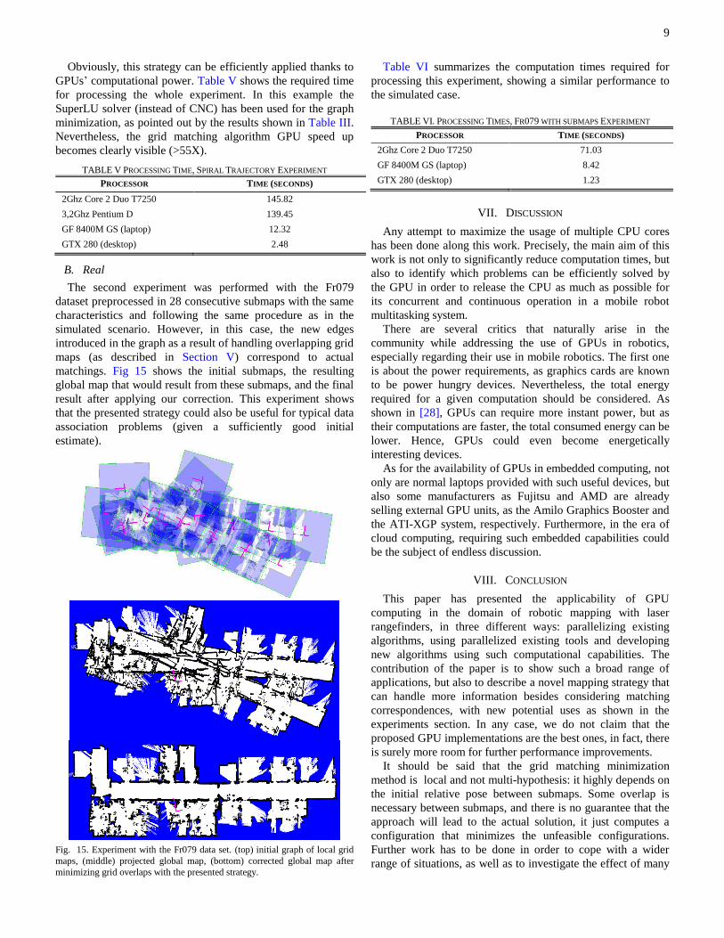
B. Real

The second experiment was performed with the Fr079

dataset preprocessed in 28 consecutive submaps with the same

characteristics and following the same procedure as in the

simulated scenario. However, in this case, the new edges

introduced in the graph as a result of handling overlapping grid

maps (as described in Section V) correspond to actual

matchings. Fig 15 shows the initial submaps, the resulting

global map that would result from these submaps, and the final

result after applying our correction. This experiment shows

that the presented strategy could also be useful for typical data

association problems (given a sufficiently good initial

estimate).

Fig. 15. Experiment with the Fr079 data set. (top) initial graph of local grid

maps, (middle) projected global map, (bottom) corrected global map after

minimizing grid overlaps with the presented strategy.

Table VI summarizes the computation times required for

processing this experiment, showing a similar performance to

the simulated case.

TABLE VI. PROCESSING TIMES, FR079 WITH SUBMAPS EXPERIMENT

PROCESSOR TIME (SECONDS)

2Ghz Core 2 Duo T7250 71.03

GF 8400M GS (laptop) 8.42

GTX 280 (desktop) 1.23

VII. DISCUSSION

Any attempt to maximize the usage of multiple CPU cores

has been done along this work. Precisely, the main aim of this

work is not only to significantly reduce computation times, but

also to identify which problems can be efficiently solved by

the GPU in order to release the CPU as much as possible for

its concurrent and continuous operation in a mobile robot

multitasking system.

There are several critics that naturally arise in the

community while addressing the use of GPUs in robotics,

especially regarding their use in mobile robotics. The first one

is about the power requirements, as graphics cards are known

to be power hungry devices. Nevertheless, the total energy

required for a given computation should be considered. As

shown in [28], GPUs can require more instant power, but as

their computations are faster, the total consumed energy can be

lower. Hence, GPUs could even become energetically

interesting devices.

As for the availability of GPUs in embedded computing, not

only are normal laptops provided with such useful devices, but

also some manufacturers as Fujitsu and AMD are already

selling external GPU units, as the Amilo Graphics Booster and

the ATI-XGP system, respectively. Furthermore, in the era of

cloud computing, requiring such embedded capabilities could

be the subject of endless discussion.

VIII. CONCLUSION

This paper has presented the applicability of GPU

computing in the domain of robotic mapping with laser

rangefinders, in three different ways: parallelizing existing

algorithms, using parallelized existing tools and developing

new algorithms using such computational capabilities. The

contribution of the paper is to show such a broad range of

applications, but also to describe a novel mapping strategy that

can handle more information besides considering matching

correspondences, with new potential uses as shown in the

experiments section. In any case, we do not claim that the

proposed GPU implementations are the best ones, in fact, there

is surely more room for further performance improvements.

It should be said that the grid matching minimization

method is local and not multi-hypothesis: it highly depends on

the initial relative pose between submaps. Some overlap is

necessary between submaps, and there is no guarantee that the

approach will lead to the actual solution, it just computes a

configuration that minimizes the unfeasible configurations.

Further work has to be done in order to cope with a wider

range of situations, as well as to investigate the effect of many

10

parameters as the submaps blurring, the weights in the

minimization cost functions, etc. to which the presented

algorithms seems quite sensitive. Nevertheless, the already

achieved speedups show that this goal is computationally

realistic and affordable, and this will be the subject of our next

coming research.

It is difficult to define some general criteria for deciding

whether to use a GPU for a certain problem. To summarize

some conditions have to be met: I) the problem should be large

enough, and involve basically the same operations, which can

be executed independently for many thousands of data items

(all the threads run the same code), II) there should be

extremely low synchronization requirements, and III) memory

transfers from and to the graphics device should be limited

compared with the amount of computation, prioritizing a few

large transfers instead of many small ones. Once these

requisites are satisfied, especial attention has to be paid to an

adequate use of device memory, as explained in section III. It

is consequently concluded that grid map operations have high

potential for being massively parallelized and future work will

also include optimization of common tasks such as blurring the

submaps and projecting local maps onto a single grid map. On

the other hand, off-the-shelf general purpose GPU solutions

(as CNC) could also have high potential applicability, yet it

requires some benchmarking suited to the specific problem

conditions and size, as remarked in section IV. At the light of

recent results [21], [25], further study of updated CPU

hardware (as Core i7) together with other probably more

efficient CPU exact solvers is also required.

Many existing open source tools and data sets have been

used in this work. Consequently, the entire C++ source code

for the algorithms presented in this paper can be found in [18],

in the spirit that it will also be useful for the community.

ACKNOWLEDGMENT

Authors thank all the open source tools and datasets

providers: CARMEN grid mapping [14], CNC [23], Alglib

[26] and SuperLU [22]. Datasets Fr079 and Fr101 have been

obtained from Radish [16] (thanks to C. Stachniss), the TORO

algorithm and its datasets are taken from [24], thanks go to G.

Grisetti.

REFERENCES

[1] S. Thrun, J. Leonard. “Simultaneous Localization and Mapping.”

Handbook of Robotics, chapter 37. Springer. Siciliano, Bruno; Khatib,

Oussama (Eds.) (2008) ISBN: 978-3-540-23957-4

[2] H. Durrant-Whyte and T. Bailey. (2006) “Simultaneous Localisation

and Mapping (SLAM): Part I The Essential Algorithms.” IEEE Robotics

and Automation Magazine 13, issue 2: pp 99–110.

[3] F. Wörsdörfer, F. Stock, E. Bayro-Corrochano and D. Hildenbrand

“Optimizations and Performance of a Robotics Grasping Algorithm

Described in Geometric Algebra”. Lecture Notes in Computer Science.

Springer Berlin/Heidelberg ISSN 0302-9743. Vol. 5856 (2009) pp 263-

271

[4] P. Michel, J. Chestnutt, S. Kagami, K. Nishiwaki, J. Kuffner, and T.

Kanade. “GPU-accelerated Real-Time 3D Tracking for Humanoid

Locomotion and Stair Climbing” Proceedings of the IEEE/RSJ

International Conference on Intelligent Robots and Systems (IROS'07),

October, 2007, pp. 463-469.

[5] B. Charmette, E. Royer, F. Chausse, "Efficient planar features matching

for robot localization using GPU," 2010 IEEE Computer Society

Conference on Computer Vision and Pattern Recognition Workshops

(CVPRW), DOI: 10.1109/CVPRW.2010.5543757 2010 pp: 16 – 23

[6] J. F. Ferreira, J. Lobo, J. Dias “Bayesian real-time perception algorithms

on GPU”. J Real-Time Image Proc. (2010) DOI 10.1007/s11554-010-

0156-7

[7] Institute for Computer Graphics and Vision, Graz University of

Technology. Gpu4Vision project available at url: www.gpu4vision.org

[8] M. Yguel, O. Aycard and C. Laugier “Efficient GPU-based

Construction of Occupancy Grids Using several Laser Range-finders.”

International Journal of Vehicle Autonomous Systems. (2008) Volume

6, Number 1-2. pp 48-83

[9] D. Borrmann, J. Elseberg, K. Lingemann, A. Nüchter, and J. Hertzberg.

“Globally consistent 3D mapping with scan matching.” Journal of

Robotics and Autonomous Systems, Elsevier Science, Volume 56, Issue

2, ISSN 0921-8890, February 2008, pp 130 – 142

[10] D. Qiu, S. May, and A. Nüchter. “GPU-accelerated Nearest Neighbor

Search for 3D Registration.” International Conference on Computer

Vision Systems (ICVS '09). LNCS 5815, Springer ISBN 978-3-642-

04666-7, Lìege Belgium, October 2009 pp 194-203

[11] ROS support for CUDA: http://www.ros.org/wiki/gpgpu

[12] A. Elfes. (1987). “Sonar-based real-world mapping and navigation.”

IEEE Journal on Robotics and Automation. Vol. 3 N. 3. pp. 249-265.

[13] Thrun S., Bücken A., Burgard W., Fox D., Fröhlinghaus T., Henning D.,

Hofmann T., Krell M., and Schmidt T. “Map learning and high-speed

navigation in RHINO.” AI-based Mobile Robots: Case Studies of

Successful Robot Systems. (1998) MIT Press.

[14] CARMEN, The Carnegie Mellon Robot Navigation Toolkit. Available

at: http://carmen.sourceforge.net/

[15] J. E. Bresenham (1965) "Algorithm for computer control of a digital

plotter", IBM Systems Journal, vol 4, N.1, pp. 25-30

[16] C. Stachniss. "Radish, The Robotics Data Set Repository." (2003).

URL: http://radish.sourceforge.net

[17] D. Rodriguez-Losada, P. de la Puente, A. Valero, P. San Segundo, M.

Hernando. “Fast Processing of Grid Maps using Graphical

Multiprocessors”.7th IFAC Symposium on Intelligent Autonomous

Vehicles (IAV) 2010. Lecce, Italy. (to appear)

[18] Source code for this paper, available at URL:

www.intelligentcontrol.es/diego/gpumapping

[19] F. Lu and E. Milios. "Globally consistent range scan alignment for

environment mapping." Autonomous Robots, 4:333–349, 1997.

[20] G. Grisetti, C. Stachniss, S. Grzonka, and W. Burgard (2007) A Tree

Parameterization for Efficiently Computing Maximum Likelihood Maps

using Gradient Descent. Robotics: Science and Systems (RSS), Atlanta,

USA.

[21] G. Grisetti, R. Kummerle, C. Stachniss, U. Frese, C. Hertzberg,

“Hierarchical optimization on manifolds for online 2D and 3D

mapping” IEEE International Conference on Robotics and Automation

(ICRA), 2010, doi: 10.1109/ROBOT.2010.5509407, pp 273 – 278

[22] J. W. Demmel, S.C. Eisenstat, J. R. Gilbert, X. S. Li and J. W. H. Liu,

“A supernodal approach to sparse partial pivoting”. SIAM J. Matrix

Analysis and Applications (1999), vol 20, n 3, pp 720-755

[23] L. Buatoisab, G. Caumona, B. Levy “Concurrent number cruncher: a

GPU implementation of a general sparse linear solver”. International

Journal of Parallel, Emergent and Distributed Systems, DOI:

10.1080/17445760802337010. Vol. 24, Issue 3, 2009 , pp 205 – 223

[24] C. Stachniss, U. Frese, G. Grisetti. "OpenSLAM." Open source SLAM

algorithms by several authors, available at url: http://www.openslam.org

[25] K. Konolige, G. Grisetti, R. Kummerle, W. Burgard, B. Limketkai, and

R. Vincent. Sparse Pose Adjustment for 2D Mapping, IROS, 10/2010,

Taipei, Taiwan.

[26] Bochkanov, S. (2010). ALGLIB software library, L-BFGS C++

implementation. http://www.alglib.net/

[27] D. Rodriguez-Losada, P. de la Puente, A. Valero, P. San Segundo, M.

Hernando. "Computation of the Optimal Relative Pose between

Overlapping Grid Maps through Discrepancy Minimization". 7th IFAC

Symposium on Intelligent Autonomous Vehicles (IAV) 2010. Lecce,

Italy. (to appear)

[28] S. Huang, S. Xiao, W. Feng. “On the energy efficiency of graphics

processing units for scientific computing.” 2009 IEEE International

Symposium on Parallel&Distributed Processing. Rome, Italy. May 23-

May 29. ISBN: 978-1-4244-3751-1