graded arm assembly language examples - …alanclements.org/armgradedexamples.pdfpurpose of using q...
TRANSCRIPT
Alan Clements ARM simulator notes Page 1
Graded ARM assembly language Examples
These examples have been created to help students with the basics of Keil’s ARM development system. I am providing
a series of examples that demonstrate the ARM’s instruction set.
These begin with very basic examples of addition. If any reader has difficulties with this material or can suggest
improvements or corrections, please email me at [email protected] and I will do my best to make the
appropriate changes.
In most examples, I present the problem in words, the basic code, and then the assembly language version. I also show
the output of the simulator at various stages during the simulation. When writing assembly language I use bold font to
indicate the destination operand (this will be in the code fragments as the assembler does not support this).
Quick Guide to Using the Keil ARM Simulator
1. Run the IDE package. I am using µVision V4.22.22.0
2. Click Project, select New Microvision Project Note that bold blue font indicates your input to the
computer and bold blue indicates the computer’s response (or option).
3. Enter filename in the File name box. Say, MyFirstExample
4. Click on Save.
5. This causes a box labelled Select Device for Target ‘Target 1’ to pop up. You now have to say which
processor family and which version you are going to use.
6. From the list of devices select ARM and then from the new list select ARM7 (Big Endian)
7. Click on OK. The box disappears. You are returned to the main µVision window.
8. We need to enter the source program. Click File. Select New and click it. This brings up an edit box
labelled Text1. We can now enter a simple program. I suggest:
AREA MyFirstExample, CODE, READONLY
ENTRY
MOV r0,#4 ;load 4 into r0
MOV r1,#5 ;load 5 into r1
ADD r2,r0,e1 ;add r0 to r1 and put the result in r2
S B S ;force infinite loop by branching to this line
END ;end of program
9. When you’ve entered the program select File then Save from the menu. This prompts you for a File
name. Use MyFirstExample.s The suffix .s indicates source code.
10. This returns you to the window now called MyFirstExample and with the code set out using ARM’s
conventions to highlight code, numbers, and comments.
11. We now have to set up the environment. Click Project in the main menu. From the pulldown list select
Manage. That will give you a new list. Select Components, Environment,Books..
12. You now get a form with three windows. Below the right hand window, select Add Files.
13. This gives you the normal Windows file view. Click on the File of type expansion arrow and select
Asm Source file (*.s*; *.src; *.a*). You should now see your own file MyFirstExample.s appear in
the window. Select this and click the Add tab. This adds your source file to the project. Then click
Close. You will now see your file in the rightmost window. Click OK to exit.
14. That’s it. You are ready to assemble the file.
15. Select Project from the top line and then click on Built target.
16. In the bottom window labelled Build Output you will see the result of the assembly process.
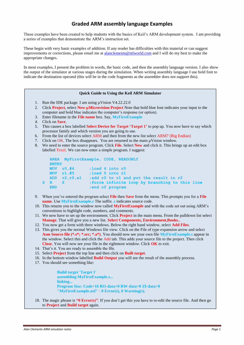
17. You should see something like:
Build target 'Target 1'
assembling MyFirstExample.s...
linking...
Program Size: Code=16 RO-data=0 RW-data=0 ZI-data=0
"MyFirstExample.axf" - 0 Error(s), 0 Warning(s).
18. The magic phrase is “0 Error(s)”. If you don’t get this you have to re-edit the source file. And then go
to Project and Build target again.
Alan Clements ARM simulator notes Page 2
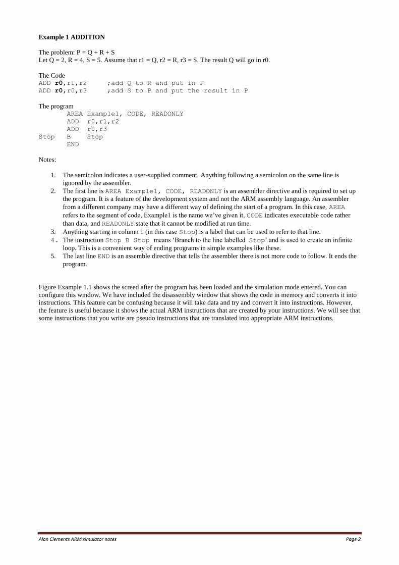
Example 1 ADDITION
The problem: P = Q + R + S
Let Q = 2, R = 4, S = 5. Assume that r1 = Q, r2 = R, r3 = S. The result Q will go in r0.
The Code ADD r0,r1,r2 ;add Q to R and put in P
ADD r0,r0,r3 ;add S to P and put the result in P
The program AREA Example1, CODE, READONLY
ADD r0,r1,r2
ADD r0,r3
Stop B Stop
END
Notes:
1. The semicolon indicates a user-supplied comment. Anything following a semicolon on the same line is
ignored by the assembler.
2. The first line is AREA Example1, CODE, READONLY is an assembler directive and is required to set up
the program. It is a feature of the development system and not the ARM assembly language. An assembler
from a different company may have a different way of defining the start of a program. In this case, AREA
refers to the segment of code, Example1 is the name we’ve given it, CODE indicates executable code rather
than data, and READONLY state that it cannot be modified at run time.
3. Anything starting in column 1 (in this case Stop) is a label that can be used to refer to that line.
4. The instruction Stop B Stop means ‘Branch to the line labelled Stop’ and is used to create an infinite
loop. This is a convenient way of ending programs in simple examples like these.
5. The last line END is an assemble directive that tells the assembler there is not more code to follow. It ends the
program.
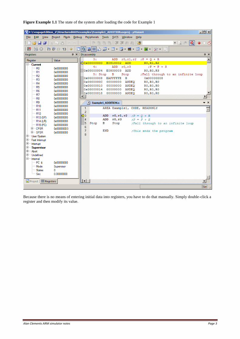
Figure Example 1.1 shows the screed after the program has been loaded and the simulation mode entered. You can
configure this window. We have included the disassembly window that shows the code in memory and converts it into
instructions. This feature can be confusing because it will take data and try and convert it into instructions. However,
the feature is useful because it shows the actual ARM instructions that are created by your instructions. We will see that
some instructions that you write are pseudo instructions that are translated into appropriate ARM instructions.
Alan Clements ARM simulator notes Page 3
Figure Example 1.1 The state of the system after loading the code for Example 1
Because there is no means of entering initial data into registers, you have to do that manually. Simply double-click a
register and then modify its value.
Alan Clements ARM simulator notes Page 4
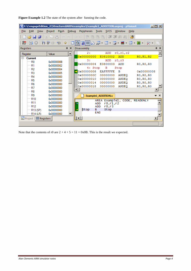
Figure Example 1.2 The state of the system after funning the code.
Note that the contents of r0 are 2 + 4 + 5 = 11 = 0x0B. This is the result we expected.
Alan Clements ARM simulator notes Page 5
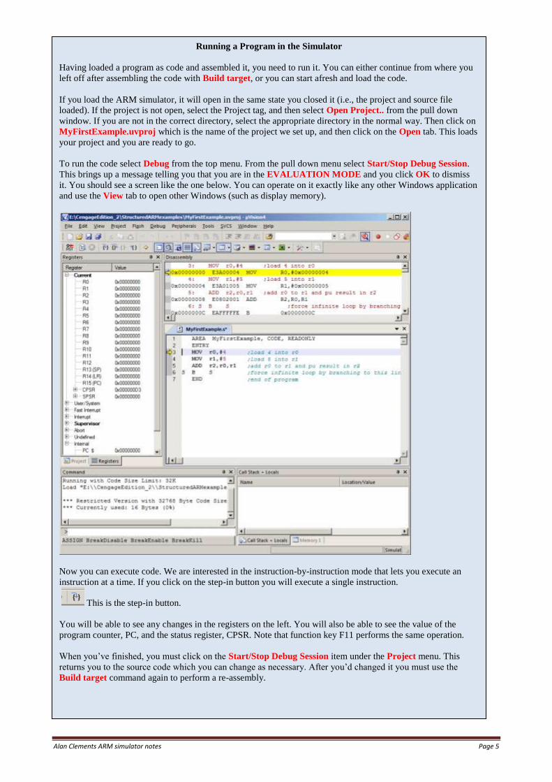
Running a Program in the Simulator
Having loaded a program as code and assembled it, you need to run it. You can either continue from where you
left off after assembling the code with Build target, or you can start afresh and load the code.
If you load the ARM simulator, it will open in the same state you closed it (i.e., the project and source file
loaded). If the project is not open, select the Project tag, and then select Open Project.. from the pull down
window. If you are not in the correct directory, select the appropriate directory in the normal way. Then click on
MyFirstExample.uvproj which is the name of the project we set up, and then click on the Open tab. This loads
your project and you are ready to go.
To run the code select Debug from the top menu. From the pull down menu select Start/Stop Debug Session.
This brings up a message telling you that you are in the EVALUATION MODE and you click OK to dismiss
it. You should see a screen like the one below. You can operate on it exactly like any other Windows application
and use the View tab to open other Windows (such as display memory).
Now you can execute code. We are interested in the instruction-by-instruction mode that lets you execute an
instruction at a time. If you click on the step-in button you will execute a single instruction.
This is the step-in button.
You will be able to see any changes in the registers on the left. You will also be able to see the value of the
program counter, PC, and the status register, CPSR. Note that function key F11 performs the same operation.
When you’ve finished, you must click on the Start/Stop Debug Session item under the Project menu. This
returns you to the source code which you can change as necessary. After you’d changed it you must use the
Build target command again to perform a re-assembly.
Alan Clements ARM simulator notes Page 6
Example 2 ADDITION
This problem is the same as Example 1. P = Q + R + S
Once again, let Q = 2, R = 4, S = 5 and assume r1 = Q, r2 = R, r3 = S. In this case, we will put the data in memory in
the form of constants before the program runs.
The Code
MOV r1,#Q ;load Q into r1
MOV r2,#R ;load R into r2
MOV r3,#S ;load S into r3
ADD r0,r1,r2 ;Add Q to R
ADD r0,r0,r3 ;Add S to (Q + R)
Here we use the instruction MOV that copies a value into a register. The value may be the contents of another register or
a literal. The literal is denoted by the # symbol. We can write, for example, MOV r7,r0, MOV r1,#25 or
MOV r5,#Time
We have used symbolic names Q, R and S. We have to relate these names to actual values. We do this with the EQU
(equate) assembler directive; for example,
Q EQU 2
Relates the name Q to the value 5. If the programmer uses Q in an expression, it is exactly the same as writing 2. The
purpose of using Q rather than 2 is to make the program more readable.
The program
AREA Example2, CODE, READONLY
MOV r1,#Q ;load r1 with the constant Q
MOV r2,#R
MOV r3,#S
ADD r0,r1,r2
ADD r0,r0,r3
Stop B Stop
Q EQU 2 ;Equate the symbolic name Q to the value 2
R EQU 4 ;
S EQU 5 ;
END
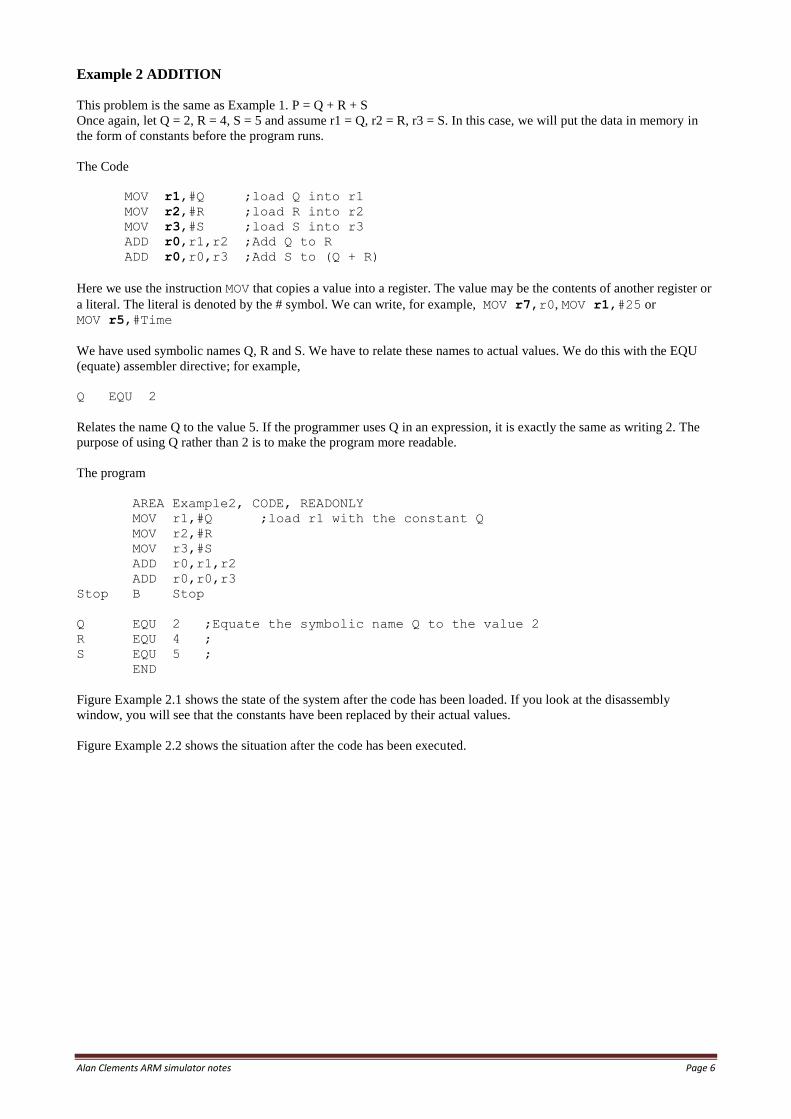
Figure Example 2.1 shows the state of the system after the code has been loaded. If you look at the disassembly
window, you will see that the constants have been replaced by their actual values.
Figure Example 2.2 shows the situation after the code has been executed.
Alan Clements ARM simulator notes Page 7
Figure Example 2.1 The state of the system after loading the code.
Figure Example 2.2 The state of the system after running the code.
Alan Clements ARM simulator notes Page 8
Example 3 ADDITION
The problem once again is P = Q + R + S. As before, Q = 2, R = 4, S = 5 and we assume that r1 = Q, r2 = R, r3 = S.
In this case, we will put the data in memory as constants before the program runs. We first use the load register,
LDR r1,Q instruction to load register r1 with the contents of memory location Q. This instruction does not exist and is
not part of the ARM’s instruction set. However, the ARM assembler automatically changes it into an actual instruction.
We call LDR r1,Q a pseudoinstruction because it behaves like a real instruction. It is indented to make the life of a
programmer happier by providing a shortcut.
The Code
LDR r1,Q ;load r1 with Q
LDR r2,R ;load r2 with R
LDR r3,S ;load r3 with S
ADD r0,r1,r2 ;add Q to R
ADD r0,r0,r3 ;add in S
STR r0,Q ;store result in Q
The program
AREA Example3, CODE, READWRITE
LDR r1,Q ;load r1 with Q
LDR r2,R ;load r2 with R
LDR r3,S ;load r3 with S
ADD r0,r1,r2 ;add Q to R
ADD r0,r3 ;add in S
STR r0,Q ;store result in Q
Stop B Stop
AREA Example3, CODE, READWRITE
P SPACE 4 ;save one word of storage
Q DCD 2 ;create variable Q with initial value 2
R DCD 4 ;create variable R with initial value 4
S DCD 5 ;create variable S with initial value 5
END
Note how we have to create a data area at the end of the program. We have reserved spaces for P, Q, R, and S. We use
the SPACE directive for S to reserve 4 bytes of memory space for the variable S. After that we reserve space for Q, R,
and S. In each case we use a DCD assembler directive to reserve a word location (4 bytes) and to initialize it. For
example,
Q DCD 2 ;create variable Q with initial value 2
means ‘call the current line Q and store the word 0x00000002 at that location.
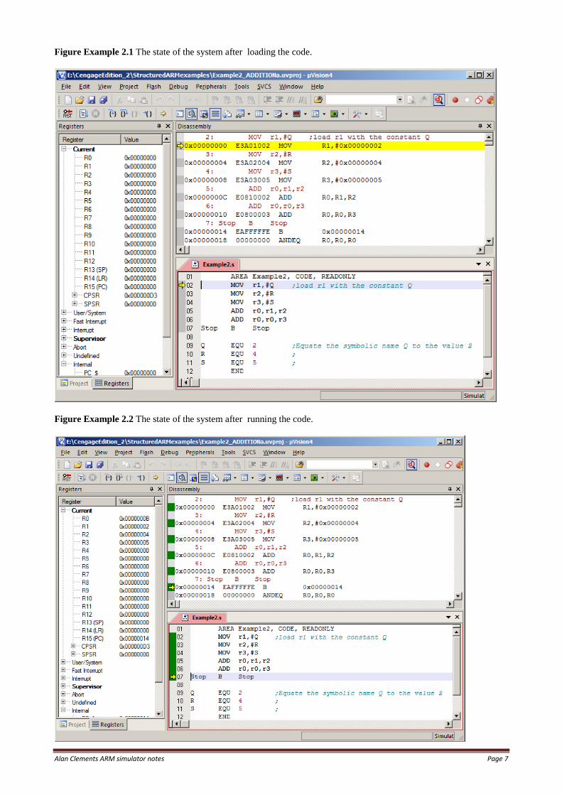
Figure Example 3.1 shows the state of the program after it has been loaded. In this case we’ve used the view memory
command to show the memory space. We have highlighted the three constants that have been pre-loaded into memory.
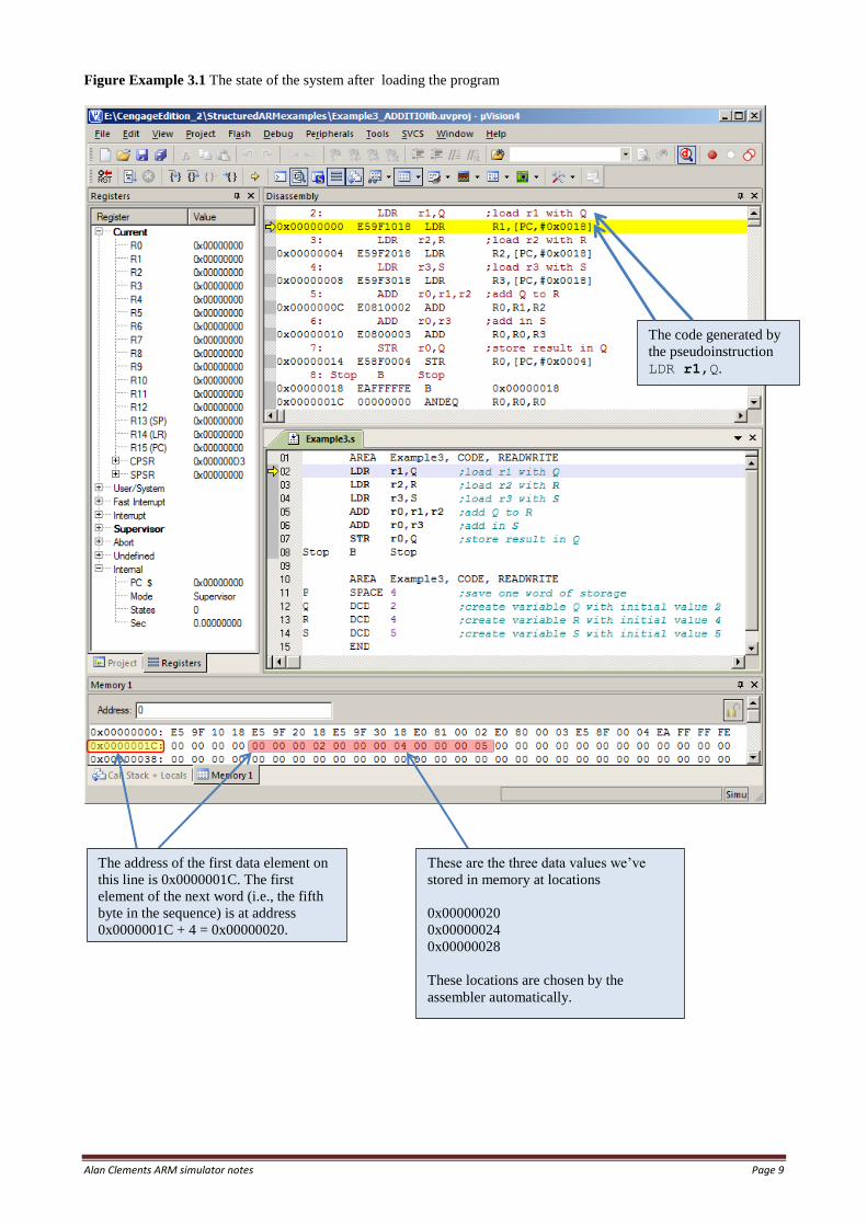
Take a look at the disassembled code. The pseudoinstruction LDR r1,Q was actually translated into the real ARM
instruction LDR r1,[PC,#0x0018]. This is still a load instruction but the addressing mode is register indirect. In
this case, the address is the contents of the program counter, PC, plus the hexadecimal offset 0x18. Note also that the
program counter is always 8 bytes beyond the address of the current instruction. This is a feature of the ARM’s
pipeline.
Consequently, the address of the operand is [PC] + 0x18 + 8 = 0 + 18 + 8 = 0x20.
If you look at the memory display area you will find that the contents of 0x20 are indeed 0x00000002.
Alan Clements ARM simulator notes Page 9
Figure Example 3.1 The state of the system after loading the program
The code generated by
the pseudoinstruction
LDR r1,Q.
These are the three data values we’ve
stored in memory at locations
0x00000020
0x00000024
0x00000028
These locations are chosen by the
assembler automatically.
The address of the first data element on
this line is 0x0000001C. The first
element of the next word (i.e., the fifth
byte in the sequence) is at address
0x0000001C + 4 = 0x00000020.
Alan Clements ARM simulator notes Page 10
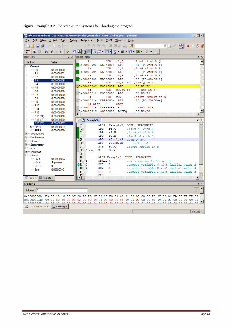
Figure Example 3.2 The state of the system after loading the program
Alan Clements ARM simulator notes Page 11
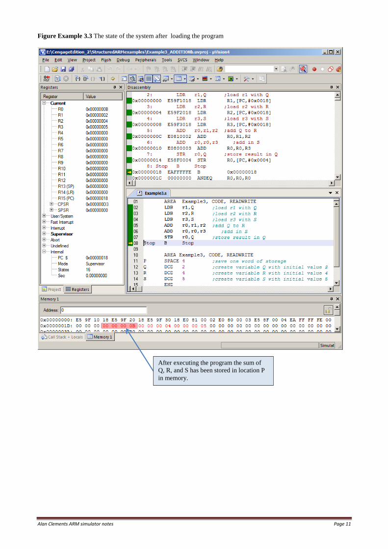
Figure Example 3.3 The state of the system after loading the program
After executing the program the sum of
Q, R, and S has been stored in location P
in memory.
Alan Clements ARM simulator notes Page 12
Example 4 ADDITION
The problem
P = Q + R + S where Q = 2, R = 4, S = 5. In this case we are going to use register indirect addressing to access the
variables. That is, we have to set up a pointer to the variables and access them via this pointer.
The Code
ADR r4,TheData ;r4 points to the data area
LDR r1,[r4,#Q] ;load Q into r1
LDR r2,[r4,#R] ;load R into r2
LDR r3,[r4,#S] ;load S into r3
ADD r0,r1,r2 ;add Q and R
ADD r0,r0,r3 ;add S to the total
STR r0,[r4,#P] ;save the result in memory
The program
AREA Example4, CODE, READWRITE
ENTRY
ADR r4,TheData ;r4 points to the data area
LDR r1,[r4,#Q] ;load Q into r1
LDR r2,[r4,#R] ;load R into r2
LDR r3,[r4,#S] ;load S into r3
ADD r0,r1,r2 ;add Q and R
ADD r0,r0,r3 ;add S to the total
STR r0,[r4,#P] ;save the result in memory
Stop B Stop
P EQU 0 ;offset for P
Q EQU 4 ;offset for Q
R EQU 8 ;offset for R
S EQU 12 ;offset for S
AREA Example4, CODE, READWRITE
TheData SPACE 4 ;save one word of storage for P
DCD 2 ;create variable Q with initial value 2
DCD 4 ;create variable R with initial value 4
DCD 5 ;create variable S with initial value 5
END
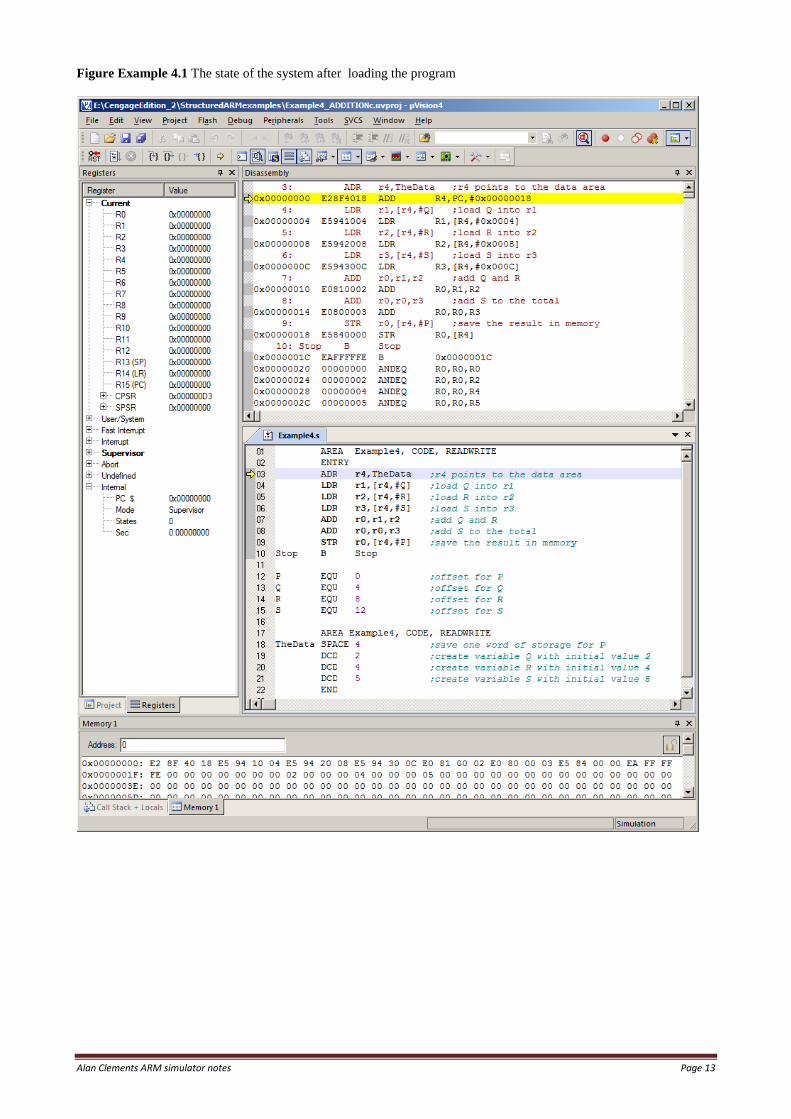
Figure Example 4.1 shows the state of the system after the program has been loaded.
I have to admit, that I would not write this code as it is presented. It is far too verbose. However, it does illustrate
several concepts.
First, the instruction ADR r4,TheData loads the address of the data region (that we have labelled TheData into
register r4. That is, r4 is pointing at the data area. If you look at the code, we have reserved four bytes for P and then
have loaded the values for Q, R and S into consecutive word location. Note that we have not labelled any of these
locations.
The instruction ADR (load an address into a register) is a pseudoinstruction. If you look at the actual disassembled code
in Figure Example 4.1 you will see that this instruction is translated into ADD r4,pc,#0x18. Instead of loading the
actual address of TheData into r4 it is loading the PC plus an offset that will give the appropriate value. Fortunately,
programmers can sleep soundly without worrying about how the ARM is going to translate an ADR into actual code –
that’s the beauty of pseudoinstructions.
When we load Q into r1 we use LDR r1,[r4,#Q]. This is an ARM load register instruction with a literal offset;
that is, Q. If you look at the EQU region, Q is equated to 4 and therefore register r1 is loaded with the data value that is
4 bytes on from where r4 is pointing. This location is, of course, where the data corresponding to Q has been stored.
Alan Clements ARM simulator notes Page 13
Figure Example 4.1 The state of the system after loading the program
Alan Clements ARM simulator notes Page 14
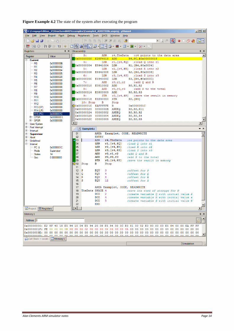
Figure Example 4.2 The state of the system after executing the program
Alan Clements ARM simulator notes Page 15
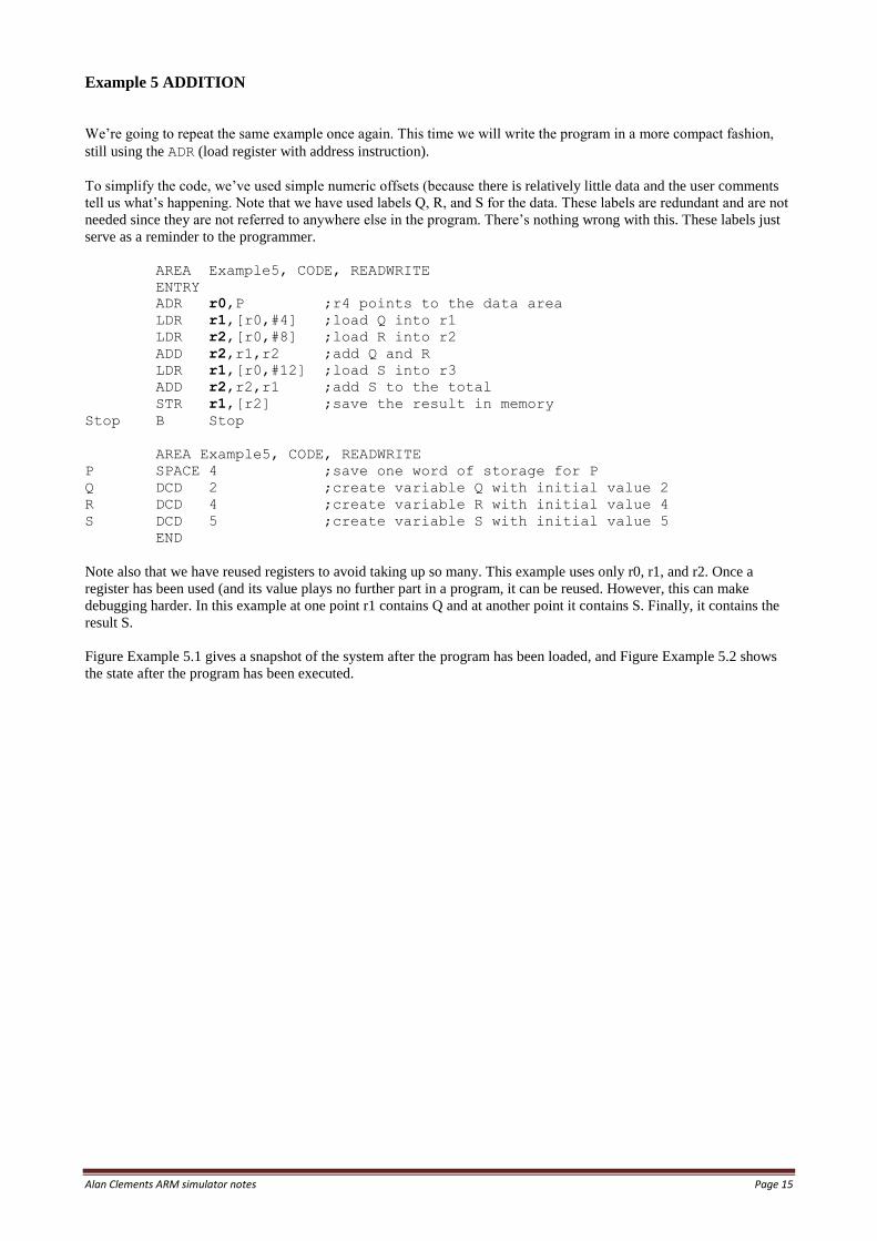
Example 5 ADDITION
We’re going to repeat the same example once again. This time we will write the program in a more compact fashion,
still using the ADR (load register with address instruction).
To simplify the code, we’ve used simple numeric offsets (because there is relatively little data and the user comments
tell us what’s happening. Note that we have used labels Q, R, and S for the data. These labels are redundant and are not
needed since they are not referred to anywhere else in the program. There’s nothing wrong with this. These labels just
serve as a reminder to the programmer.
AREA Example5, CODE, READWRITE
ENTRY
ADR r0,P ;r4 points to the data area
LDR r1,[r0,#4] ;load Q into r1
LDR r2,[r0,#8] ;load R into r2
ADD r2,r1,r2 ;add Q and R
LDR r1,[r0,#12] ;load S into r3
ADD r2,r2,r1 ;add S to the total
STR r1,[r2] ;save the result in memory
Stop B Stop
AREA Example5, CODE, READWRITE
P SPACE 4 ;save one word of storage for P
Q DCD 2 ;create variable Q with initial value 2
R DCD 4 ;create variable R with initial value 4
S DCD 5 ;create variable S with initial value 5
END
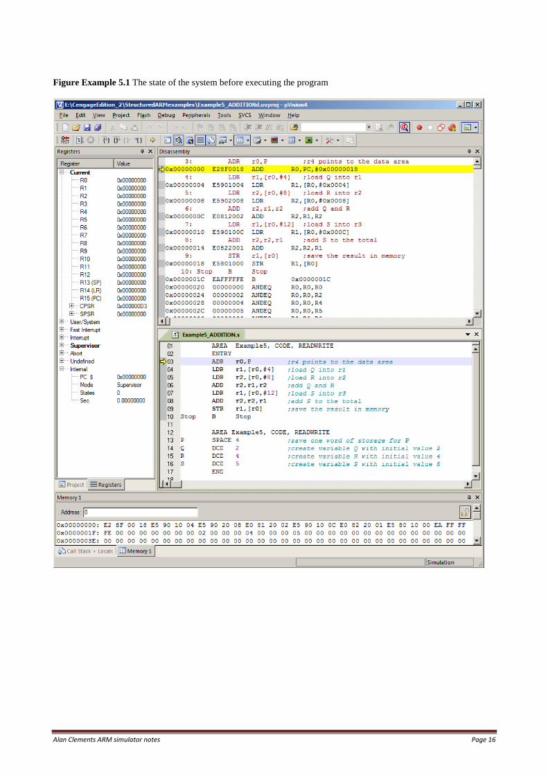
Note also that we have reused registers to avoid taking up so many. This example uses only r0, r1, and r2. Once a
register has been used (and its value plays no further part in a program, it can be reused. However, this can make
debugging harder. In this example at one point r1 contains Q and at another point it contains S. Finally, it contains the
result S.
Figure Example 5.1 gives a snapshot of the system after the program has been loaded, and Figure Example 5.2 shows
the state after the program has been executed.
Alan Clements ARM simulator notes Page 16
Figure Example 5.1 The state of the system before executing the program
Alan Clements ARM simulator notes Page 17
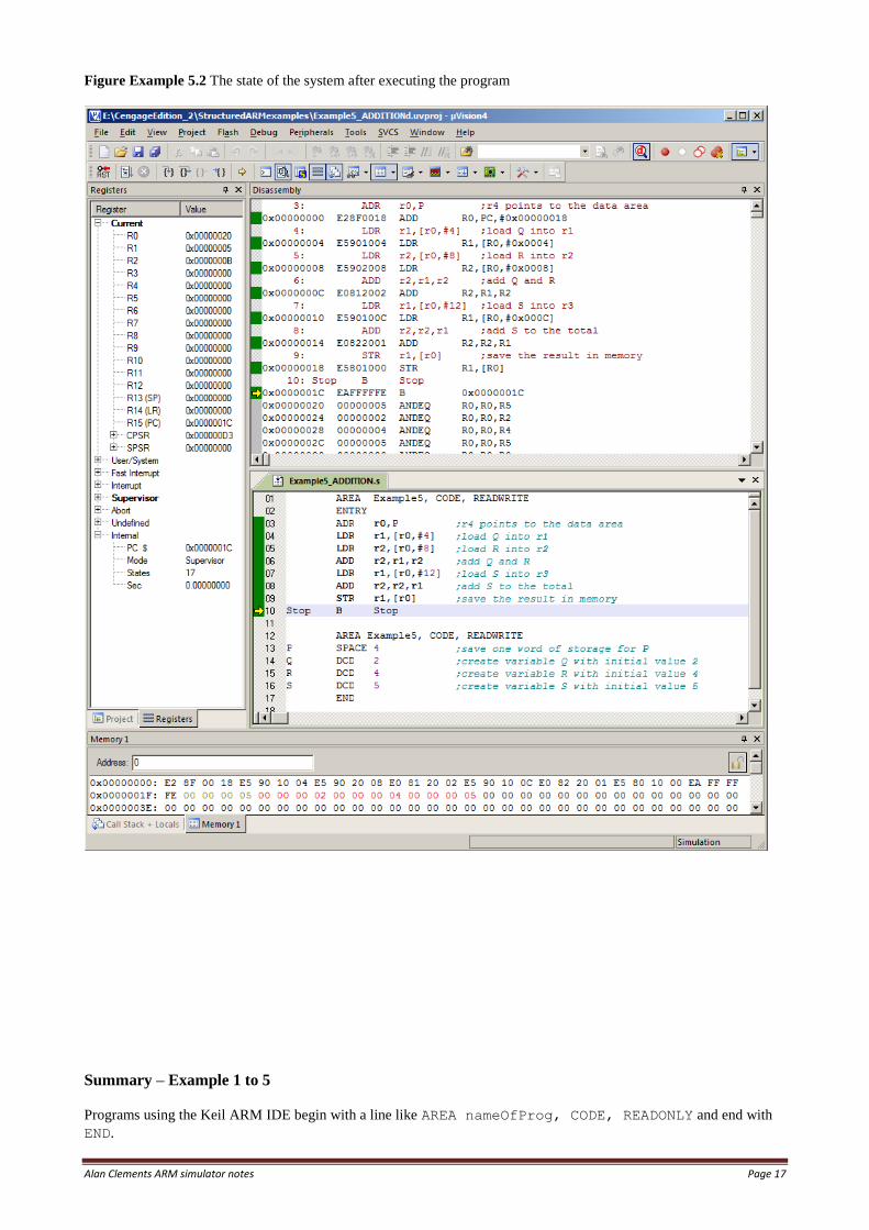
Figure Example 5.2 The state of the system after executing the program
Summary – Example 1 to 5
Programs using the Keil ARM IDE begin with a line like AREA nameOfProg, CODE, READONLY and end with
END.

Alan Clements ARM simulator notes Page 18
You can store data in memory with the DCD (define constant) before the program runs.
You can write ADD r0,r1,#4 or ADD r0,r1,K1. However, if you do use a symbolic name like K1, you
have to use an EQU statement to equate it (link it) to its actual value.
Some instructions are pseudoinstructions. They are not actual ARM instructions but a form of shorthand that is
automatically translated into one or more ARM instructions.
The instruction MOV r1,r2 or MOV r1,#literal has two operands and moves the contents of a register
or a literal into a register.
Alan Clements ARM simulator notes Page 19
Example 6 Arithmetic Expressions
The problem
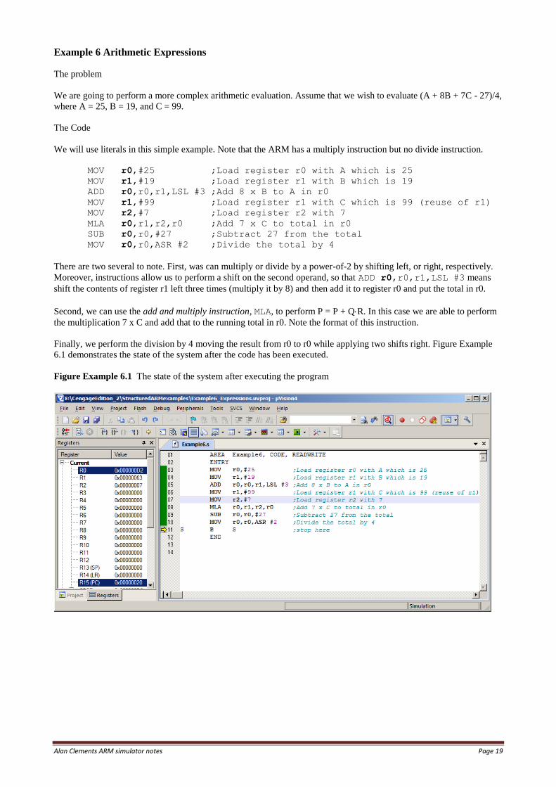
We are going to perform a more complex arithmetic evaluation. Assume that we wish to evaluate (A + 8B + 7C - 27)/4,
where A = 25, B = 19, and C = 99.
The Code
We will use literals in this simple example. Note that the ARM has a multiply instruction but no divide instruction.
MOV r0,#25 ;Load register r0 with A which is 25
MOV r1,#19 ;Load register r1 with B which is 19
ADD r0,r0,r1,LSL #3 ;Add 8 x B to A in r0
MOV r1,#99 ;Load register r1 with C which is 99 (reuse of r1)
MOV r2,#7 ;Load register r2 with 7
MLA r0,r1,r2,r0 ;Add 7 x C to total in r0
SUB r0,r0,#27 ;Subtract 27 from the total
MOV r0,r0,ASR #2 ;Divide the total by 4
There are two several to note. First, was can multiply or divide by a power-of-2 by shifting left, or right, respectively.
Moreover, instructions allow us to perform a shift on the second operand, so that ADD r0,r0,r1,LSL #3 means
shift the contents of register r1 left three times (multiply it by 8) and then add it to register r0 and put the total in r0.
Second, we can use the add and multiply instruction, MLA, to perform P = P + QR. In this case we are able to perform
the multiplication 7 x C and add that to the running total in r0. Note the format of this instruction.
Finally, we perform the division by 4 moving the result from r0 to r0 while applying two shifts right. Figure Example
6.1 demonstrates the state of the system after the code has been executed.
Figure Example 6.1 The state of the system after executing the program
Alan Clements ARM simulator notes Page 20
Example 7 Logical Operations
Logical operations are virtually the same as arithmetic operations from the programmer’s point of view. The principal
differences being that logical operations do not create a carry-out (apart from shift operations), and you don’t have to
worry about negative numbers. Logical operations are called bitwise because they act on individual bits. Basic or
fundamental logical operations are:
NOT Invert bits ci = ai
AND Logical and ci = aibi
OR Logical OR ci = ai + bi
Derived logical operations that can be expressed in terms of fundaments operations are (this is not an exhaustive list):
XOR Exclusive OR ci = aibi+ aibi
NAND NOT AND ci = aibi
NOR NOT OR ci = ai + bi
Shift operations are sometimes groups with logical operations and sometime they are not. This is because they are not
fundamental Boolean operations but they are operations on bits. A shift operation moves all the bits of a word one or
more places left or right. Typical shift operations are:
LSL Logical shift left Shift the bits left. A 0 enters at the right hand position and the bit in the left hand
position is copied into the carry bit.
LSR Logical shift right Shift the bits right. A 0 enters at the left hand position and the bit in the right hand
position is copied into the carry bit.
ROL Rotate left Shift the bits left. The bit shifted out of the left hand position is copied into the right
hand position. No bit is lost.
ROR Rotate right Shift the bits right. The bit shifted out of the right hand position is copied into the left
hand position. No bit is lost.
Some microprocessors include other logical operations. These aren’t needed and can be synthesized using other
operations.
Bit Set The bit set operation allows you to set bit i of a word to 1.
Bit Clear The bit clear operation allows you to clear bit i of a word to 0.
Bit Toggle The bit toggle operation allows you to complement bit i of a word to its complement.
ARM Logical Operations
Few microprocessors implement all the above logical operations. Some microprocessors implement special-purpose
logical operations as we shall see. The ARM’s logical operations are:
MVN MVN r0,r1 r0 = r1
AND AND r0,r1,r2 r0 = r1 r2
ORR OR r0,r1,r2 r0 = r1 + r2
EOR XOR r0,r1,r2 r0 = r1 r2
BIC BIC r0,r1,r2 r0 = r1 r2
LSL MOV r0,r1,LSL r2 r1 is shifted left by the number of places in r2
LSR MOV r0,r1,LSR r2 r1 is shifted right by the number of places in r2
The two unusual instructions are MVN (move negated) and BIC (clear bits). The move negated instruction acts rather
like a move instruction (MOV), except that the bits are inverted. Note that the bits in the source register remain
unchanged. The BIC instruction clears bits of the first operands when bits of the destination operand are set. This
operation is equivalent to an AND between the first and negated second operand. For example, in 8 bits the operation
BIC r0,r1,r2 (with r1 = 00001111 and r2 = 11001010) would result in r0 = 11000000. This instruction is
sometimes called clear ones corresponding.
The problem
Let’s perform a simple Boolean operation to calculate the bitwise calculation of F = AB + CD.
Assume that A, B, C, D are in r1, r2, r3, r4, respectively.
Alan Clements ARM simulator notes Page 21
The Code
AND r0,r1,r2 ;r0 = AB
AND r3,r3,r4 ;r3 = CD
MVN r3,r3 ;r3 = CD
ORR r0,r0,r3 ;r0 = AB + CD
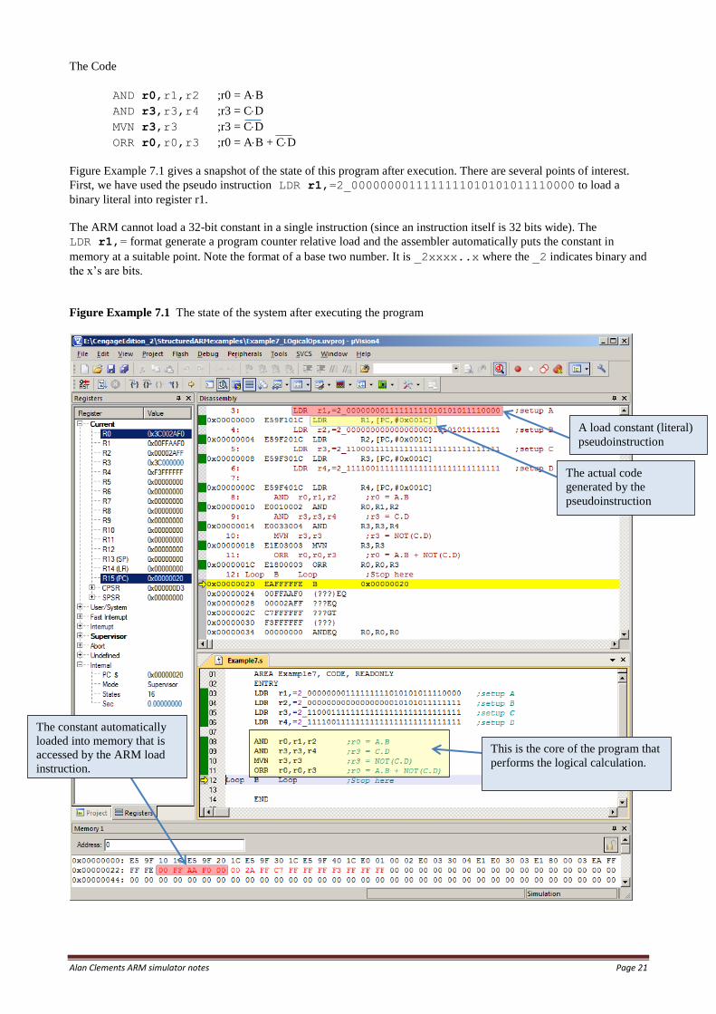
Figure Example 7.1 gives a snapshot of the state of this program after execution. There are several points of interest.
First, we have used the pseudo instruction LDR r1,=2_0000000011111111010101011110000 to load a
binary literal into register r1.
The ARM cannot load a 32-bit constant in a single instruction (since an instruction itself is 32 bits wide). The
LDR r1,= format generate a program counter relative load and the assembler automatically puts the constant in
memory at a suitable point. Note the format of a base two number. It is _2xxxx..x where the _2 indicates binary and
the x’s are bits.
Figure Example 7.1 The state of the system after executing the program
A load constant (literal)
pseudoinstruction
The actual code
generated by the
pseudoinstruction
The constant automatically
loaded into memory that is
accessed by the ARM load
instruction.
This is the core of the program that
performs the logical calculation.
Alan Clements ARM simulator notes Page 22
Example 8 A More Complex Logical Operation
Suppose we have three words P, Q and R. We are going to apply logical operations to subfields (bit fields) of these
registers. We’ll use 16-bit arithmetic for simplicity.
Suppose that we have three 6-bit bit fields in Q, R, and R as illustrated below. The bit fields are in red and are not in the
same position in each word. A bit field is a consecutive sequence of bits that forms a logic entity. Often they are data
fields packed in a register, or they may be graphical elements in a display (a row of pixels). However, the following
example demonstrates the type of operation you may have to perform on bits.
P = p15 p14 p13 p12 p11 p10 p9 p8 p7 p6 p5 p4 p3 p2 p1 p0 = 0010000011110010
Q = q15 q14 q13 q12 q11 q10 q9 q8 q7 q6 q5 q4 q3 q2 q1 q0 = 0011000011110000
R = r15 r14 r13 r12 r11 r10 r9 r8 r7 r6 r5 r4 r3 r2 r1 r0 = 1100010011111000
In this example we are going to calculate F = (P + Q R) 111110 using the three 6-bit bit fields.
Assuming that P, Q, and R are in registers r1, r2, and r3, respectively, we first have to isolate the required bit fields.
Since we are going to assume that the original data is in memory, it doesn’t matter if we modify these registers. In each
case we use a move instruction and right shift the register by the number of placed required to right-justify the bit field.
MOV r1,r1,LSR #9 ;right justify P
MOV r2,r2,LSR #1 ;right justify Q
MOV r3,r3,LSR #5 ;right justify R
We now have
P = 0 0 0 0 0 0 0 0 0 0 p15 p14 p13 p12 p11 p10 p9 = 0000000000010000
Q = 0 q15 q14 q13 q12 q11 q10 q9 q8 q7 q6 q5 q4 q3 q2 q1 = 0001100001111000
R = 0 0 0 0 0 r15 r14 r13 r12 r11 r10 r9 r8 r7 r6 r5 = 0000011000100111
We also want to ensure that all the other bits of each register are zero. We can use a logical AND operation for this.
Note that 0x3F is the 6-bit mask 111111. We could have used 2_111111
AND r1,r1,#0x3F ;convert P to six significant bits right-justified
AND r2,r2,#0x3F ;do Q
AND r3,r3,#0x3F ;do R
The now leaves us with
P = 0 0 0 0 0 0 0 0 0 0 p14 p13 p12 p11 p10 p9 = 0000000000010000
Q = 0 0 0 0 0 0 0 0 0 0 q6 q5 q4 q3 q2 q1 = 0000000000111000
R = 0 0 0 0 0 0 0 0 0 0 r10 r9 r8 r7 r6 r5 = 0000000000100111
Now we can do the calculation.
EOR r2,r2,r3 ;Calculate Q R
ORR r2,r2,r1 ;Logical OR with r1 to get (P + Q R)
AND r3,r3,#0x3E ;And with 111110 to get (P + Q R) 111110
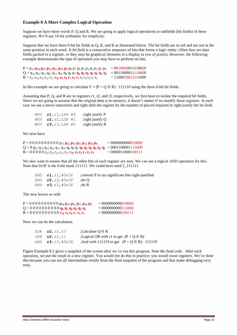
Figure Example 8.1 gives a snapshot of the screen after we’ve run this program. Note the final code. After each
operation, we put the result in a new register. You would not do this in practice; you would reuse registers. We’ve done
this because you can see all intermediate results from the final snapshot of the program and that make debugging very
easy.
Alan Clements ARM simulator notes Page 23
Figure Example 8.1 The state of the system after executing the program
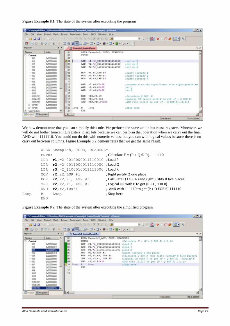
We now demonstrate that you can simplify this code. We perform the same action but reuse registers. Moreover, we
will do not bother truncating registers to six bits because we can perform that operation when we carry out the final
AND with 1111110. You could not do this with numeric values, but you can with logical values because there is no
carry out between columns. Figure Example 8.2 demonstrates that we get the same result.
AREA Example8, CODE, READONLY
ENTRY ;Calculate F = (P + Q R) 111110
LDR r1,=2_0010000011110010 ;Load P
LDR r2,=2_0011000011110000 ;Load Q
LDR r3,=2_1100010011111000 ;Load R
MOV r2,r2,LSR #1 ;Right justify Q one place
EOR r2,r2,r1, LSR #5 ;Calculate Q EOR R (and right justify R five places)
ORR r2,r2,r1, LSR #9 ;Logical OR with P to get (P + Q EOR R)
AND r2,r2,#0x3F ; AND with 111110 to get (P + Q EOR R).111110
Loop B Loop ;Stop here
END
Figure Example 8.2 The state of the system after executing the simplified program

Alan Clements ARM simulator notes Page 24
Example 9 Conditional Expressions TO BE COMPLETED