gradient boosting for multi-step forecasting · which weak learner for lk? p-splines? least-squares...
TRANSCRIPT

Gradient boosting for
multi-step forecasting
Souhaib Ben TaiebMachine Learning Group
Rob J HyndmanBusiness & Economic Forecasting Unit
Multi-step time series forecasting
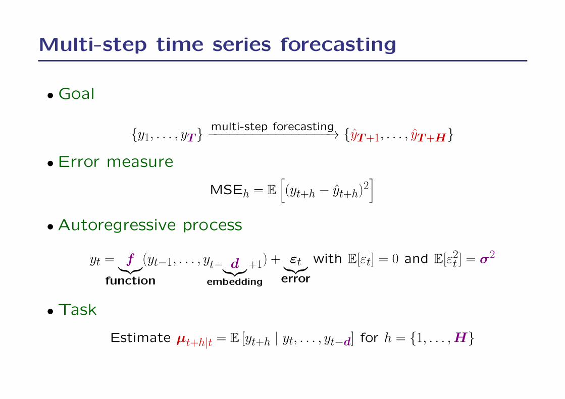
•Goal
{y1, . . . , yT }multi-step forecasting−−−−−−−−−−−−−−−−→ {yT+1, . . . , yT+H}
• Error measure
MSEh = E[(yt+h − yt+h)2
]• Autoregressive process
yt = f︸︷︷︸function
(yt−1, . . . , yt− d︸︷︷︸embedding
+1) + εt︸︷︷︸error
with E[εt] = 0 and E[ε2t ] = σ2
•Task
Estimate µt+h|t = E [yt+h | yt, . . . , yt−d] for h = {1, . . . ,H}
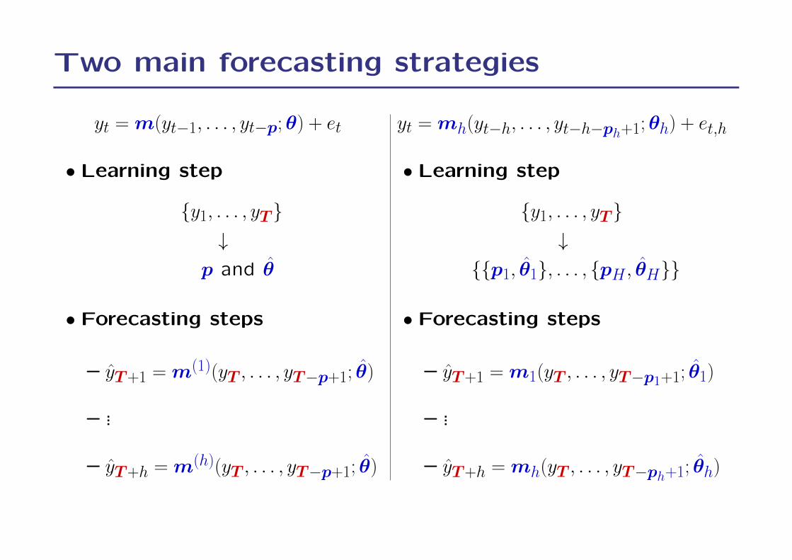
Two main forecasting strategies
yt = m(yt−1, . . . , yt−p;θ) + et
• Learning step
{y1, . . . , yT }↓
p and θ
• Forecasting steps
– yT+1 = m(1)(yT , . . . , yT−p+1; θ)
– ...
– yT+h = m(h)(yT , . . . , yT−p+1; θ)
yt = mh(yt−h, . . . , yt−h−ph+1;θh) + et,h
• Learning step
{y1, . . . , yT }↓
{{p1, θ1}, . . . , {pH , θH}}
• Forecasting steps
– yT+1 = m1(yT , . . . , yT−p1+1; θ1)
– ...
– yT+h = mh(yT , . . . , yT−ph+1; θh)

The rectify strategy ?
yt = g(h)(yt−h, . . . , yt−h−p+1;θ)︸ ︷︷ ︸recursive (linear)
+ rh(yt−h, . . . , yt−h−ph+1;γh)︸ ︷︷ ︸direct
+et,h
• Learning steps
{y1, . . . , yT } → {{p, θ}, {p1, γ1}, . . . , {pH , γH}}
• Forecasting steps
– yT+1 =
recursive (linear)︷ ︸︸ ︷g(1)(yT , . . . , yT−p+1; θ) +
direct︷ ︸︸ ︷r1(yT , . . . , yT−p1+1; γ1)
– ...
– yT+h = g(h)(yT , . . . , yT−p+1; θ) + rh(yT , . . . , yT−ph+1; γh)

RFY−KNN
Time
Val
ues
5 10 15 20 25
−0.
4−
0.3
−0.
2−
0.1
0.0
0.1
0.2

RFY−KNN
Time
Val
ues
5 10 15 20 25
−0.
4−
0.3
−0.
2−
0.1
0.0
0.1
0.2
g(h)(xt)

RFY−KNN
Time
Val
ues
5 10 15 20 25
−0.
4−
0.3
−0.
2−
0.1
0.0
0.1
0.2
g(h)(xt)+ mh(xt)
−16 −45 25 −49 −53 4792 −61 −29 −93 251 8130 93 −7 118 −7 37 −49 −29 −35 −64

RFY−MLP
Time
Val
ues
5 10 15 20 25
−0.
4−
0.3
−0.
2−
0.1
0.0
0.1
0.2

RFY−MLP
Time
Val
ues
5 10 15 20 25
−0.
4−
0.3
−0.
2−
0.1
0.0
0.1
0.2
g(h)(xt)

RFY−MLP
Time
Val
ues
5 10 15 20 25
−0.
4−
0.3
−0.
2−
0.1
0.0
0.1
0.2
g(h)(xt)+ mh(xt)
2.50 −2.53 18.58 −6.77 −6.12 216.04 −47.50 −25.97 −24.72 −99.85 1163.18 97.04 −33.96 144.01 −25.47 0.08 −29.30 39.28 −11.90 −24.89
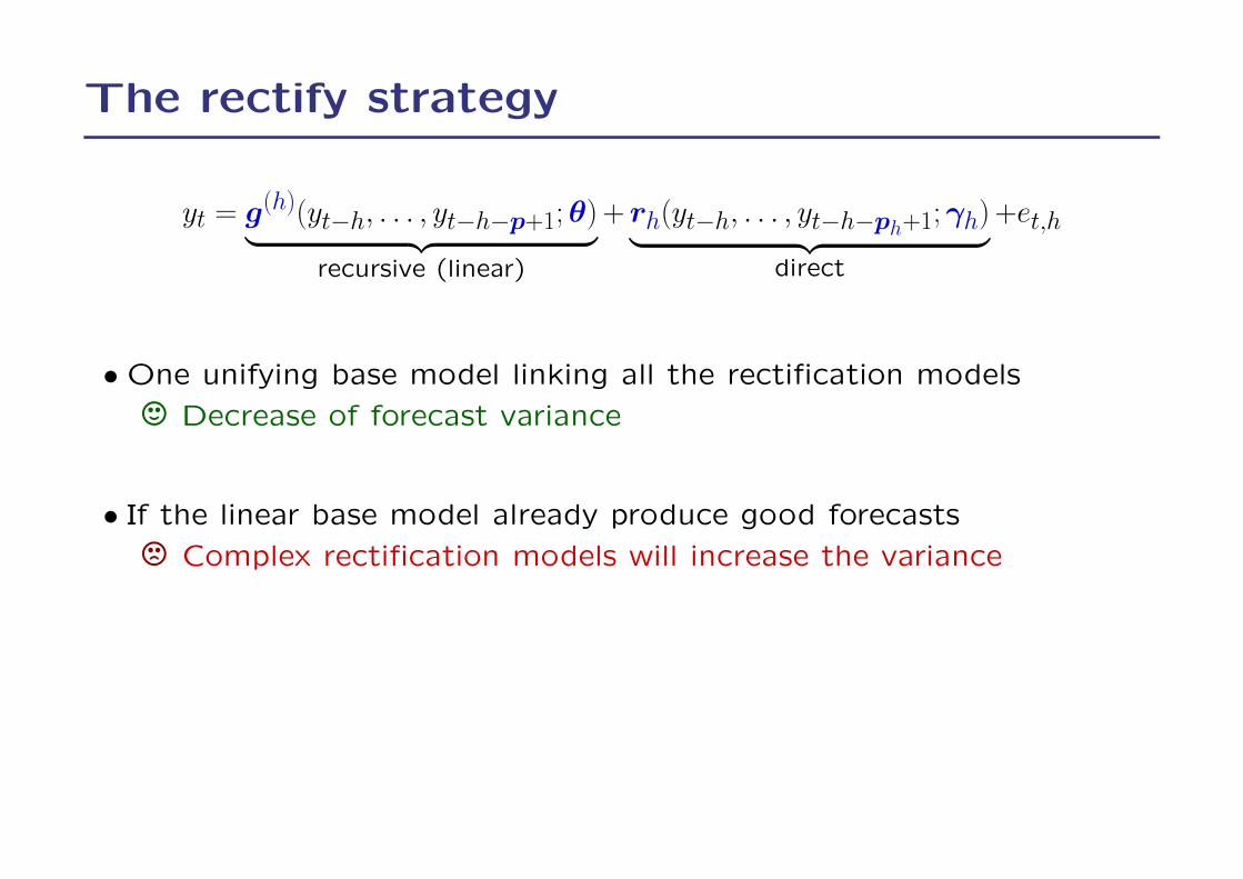
The rectify strategy
yt = g(h)(yt−h, . . . , yt−h−p+1;θ)︸ ︷︷ ︸recursive (linear)
+ rh(yt−h, . . . , yt−h−ph+1;γh)︸ ︷︷ ︸direct
+et,h
• One unifying base model linking all the rectification models
, Decrease of forecast variance
• If the linear base model already produce good forecasts
/ Complex rectification models will increase the variance
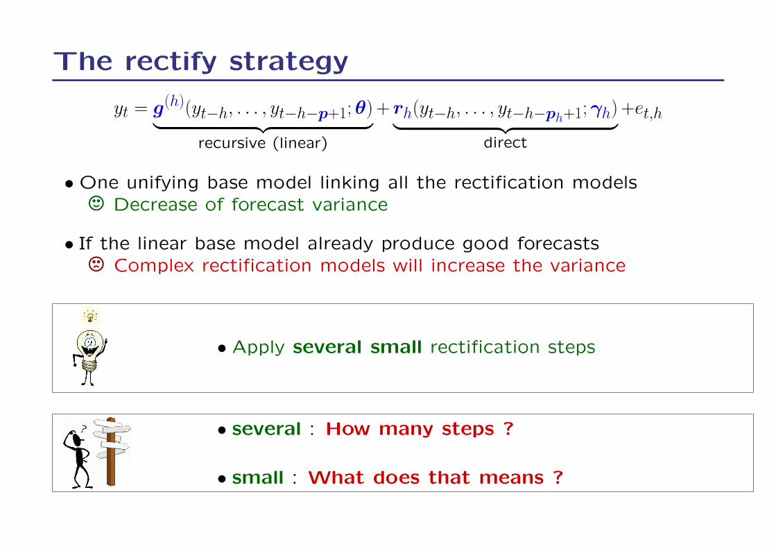
The rectify strategy
yt = g(h)(yt−h, . . . , yt−h−p+1;θ)︸ ︷︷ ︸recursive (linear)
+ rh(yt−h, . . . , yt−h−ph+1;γh)︸ ︷︷ ︸direct
+et,h
• One unifying base model linking all the rectification models, Decrease of forecast variance
• If the linear base model already produce good forecasts/ Complex rectification models will increase the variance
• Apply several small rectification steps
• several : How many steps ?
• small : What does that means ?

The BOOST strategy
• Apply a Boosting procedure for each rectification model
• Boosting ??
– Weak learning algorithm (small)
– Use the weak learner several times to build the final model→ Improve the performance at each iteration→ Early stopping to avoid overfitting (several)
– Effective Machine Learning algorithm
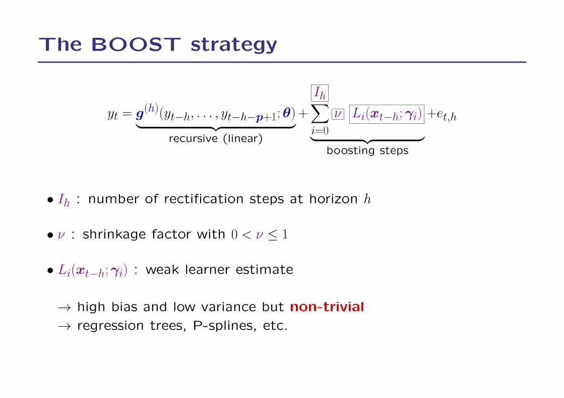
The BOOST strategy
yt = g(h)(yt−h, . . . , yt−h−p+1;θ)︸ ︷︷ ︸recursive (linear)
+
Ih∑i=0
ν Li(xt−h;γi)︸ ︷︷ ︸boosting steps
+et,h
• Ih : number of rectification steps at horizon h
• ν : shrinkage factor with 0 < ν ≤ 1
• Li(xt−h;γi) : weak learner estimate
→ high bias and low variance but non-trivial
→ regression trees, P-splines, etc.
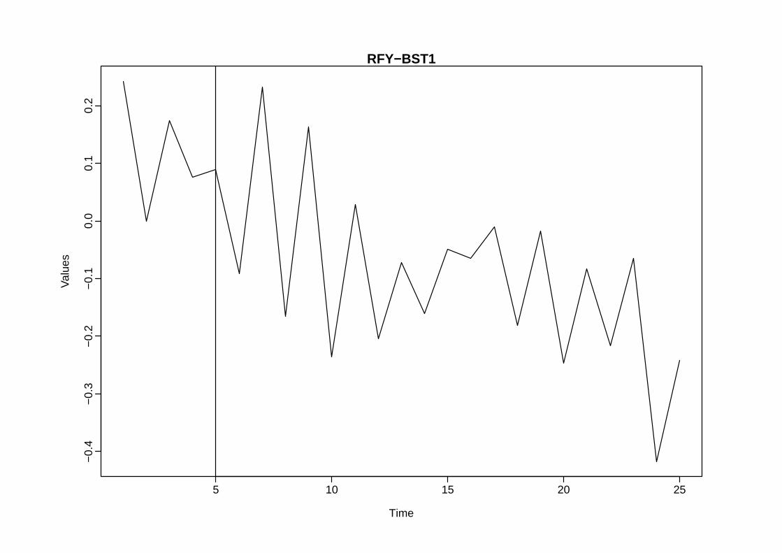
RFY−BST1
Time
Val
ues
5 10 15 20 25
−0.
4−
0.3
−0.
2−
0.1
0.0
0.1
0.2

RFY−BST1
Time
Val
ues
5 10 15 20 25
−0.
4−
0.3
−0.
2−
0.1
0.0
0.1
0.2
g(h)(xt)

BOOST (RFY−BST1)
Time
Val
ues
5 10 15 20 25
−0.
4−
0.2
0.0
0.2
17 −22 18 −29 16 695 20 37 23 84 1254 −59 11 −68 8 24 7 23 1 3
g(h)(xt)+ ∑i=0
IhνLi(xt, γi)
I1 I2 I3 I4 I5 I6 I7 I8 I9 I10 I11 I12 I13 I14 I15 I16 I17 I18 I19 I20
1 1 1 1 1 1 1 1 1 1 1 1 1 1 1 1 1 1 1 1

BOOST (RFY−BST1)
Time
Val
ues
5 10 15 20 25
−0.
4−
0.2
0.0
0.2
24.4 −21.8 21.1 −28.6 16.2 694.9 3.2 −4.4 −60.0 −99.8 5005.5 −30.3 −60.4 0.3 −42.3 −68.9 −43.9 154.9 −20.6 3.0
g(h)(xt)+ ∑i=0
IhνLi(xt, γi)
I1 I2 I3 I4 I5 I6 I7 I8 I9 I10 I11 I12 I13 I14 I15 I16 I17 I18 I19 I20
8 1 5 1 1 1 23 32 59 59 67 48 74 42 99 99 99 99 99 1

BOOST (RFY−BST1)
Time
Val
ues
5 10 15 20 25
−0.
4−
0.2
0.0
0.2
24.4 −21.8 21.1 −28.6 16.2 694.9 3.2 −4.4 −60.0 −99.8 5005.5 −30.3 −60.4 0.3 −48.9 −64.2 −50.0 224.6 −24.6 3.0
g(h)(xt)+ ∑i=0
IhνLi(xt, γi)
I1 I2 I3 I4 I5 I6 I7 I8 I9 I10 I11 I12 I13 I14 I15 I16 I17 I18 I19 I20
8 1 5 1 1 1 23 32 59 59 67 48 74 42 199 199 199 199 199 1

BOOST (RFY−BST1)
Time
Val
ues
5 10 15 20 25
−0.
4−
0.2
0.0
0.2
24.4 −21.8 21.1 −28.6 16.2 694.9 3.2 −4.4 −60.0 −99.8 5005.5 −30.3 −60.4 0.3 −75.1 −72.5 −76.3 286.5 −32.9 3.0
g(h)(xt)+ ∑i=0
IhνLi(xt, γi)
I1 I2 I3 I4 I5 I6 I7 I8 I9 I10 I11 I12 I13 I14 I15 I16 I17 I18 I19 I20
8 1 5 1 1 1 23 32 59 59 67 48 74 42 989 998 1000 1000 1000 1

Algorithm 1 Component-wise gradient boosting ?
1: {y1, . . . , yT} → {(xt−h, yt)}Tt=1 → zt = yt −m(h)(xt−h) → {(xt−h, zt)}Tt=1
2: Ih : number of boosting iterations and 0 < ν ≤ 1: shrinkage parameter
3: F (0)(xt) = L0(xt) = z = 1T
∑Tt=1 zt
4: for i← 1, . . . , Ih do
5: zit = −12∂(zt−F (xt))
2
∂F (xt)
∣∣∣∣F (xt)=F
(i−1)p (xt)
= (zt − F (i−1)(xt))
6: for k ← 1, . . . , K do
7: {(xt, zit)}Tt=1Regression with weak learner Lk−−−−−−−−−−−−−−−−−−−−−−−−→ Lk(xt; γk)
8: end for
9: ki = argmin1≤k≤K
∑Tt=1[zit − Lk(xt; γk)]2
10: F (i)(xt) = F (i−1)(xt) + νLki(xt; γki)
11: end for
12: F (xt) = L0(xt) +
Ih∑i=1
νLki(xt; γki)
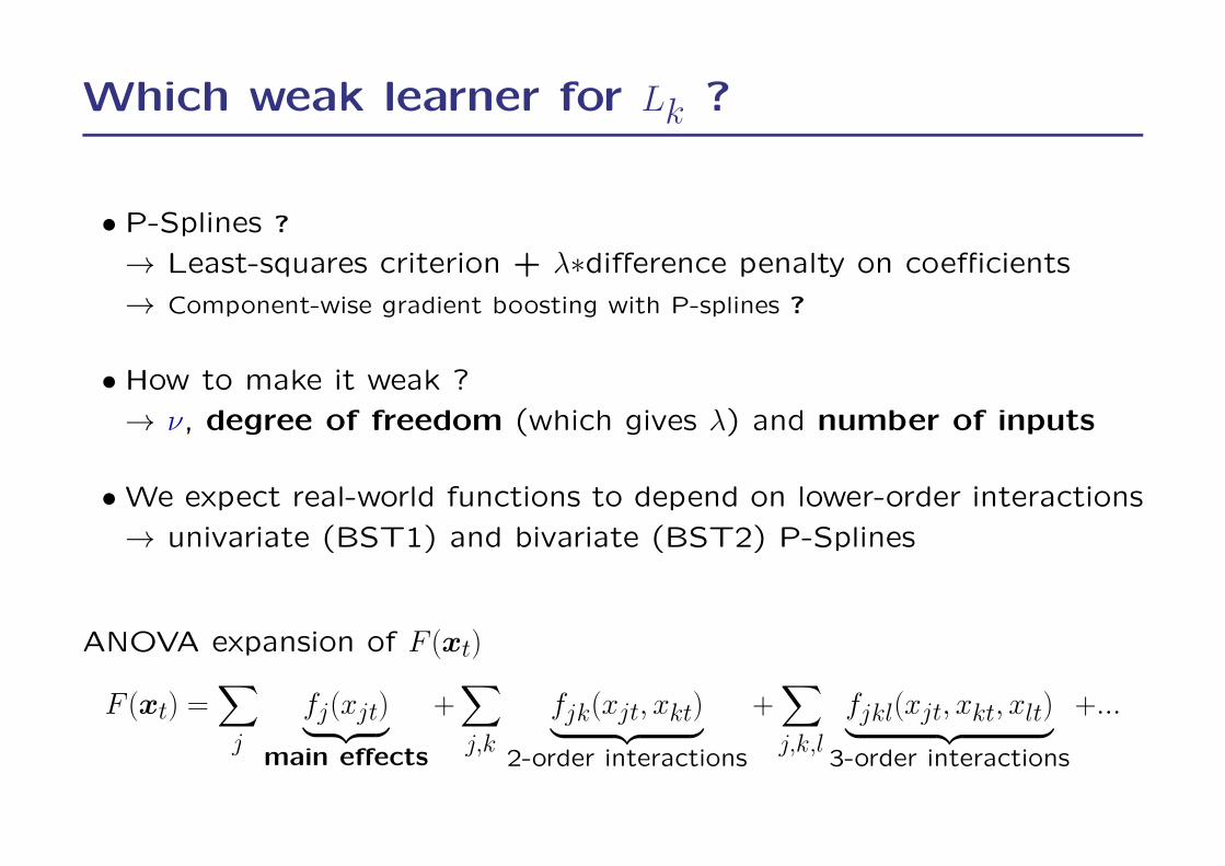
Which weak learner for Lk ?
• P-Splines ?
→ Least-squares criterion + λ∗difference penalty on coefficients
→ Component-wise gradient boosting with P-splines ?
• How to make it weak ?
→ ν, degree of freedom (which gives λ) and number of inputs
•We expect real-world functions to depend on lower-order interactions
→ univariate (BST1) and bivariate (BST2) P-Splines
ANOVA expansion of F (xt)
F (xt) =∑j
fj(xjt)︸ ︷︷ ︸main effects
+∑j,k
fjk(xjt, xkt)︸ ︷︷ ︸2-order interactions
+∑j,k,l
fjkl(xjt, xkt, xlt)︸ ︷︷ ︸3-order interactions
+...

Simulation experiments
• STAR (Smooth Transition Autoregressive) model
yt = 0.3yt−1+0.6yt−2+(0.1−0.9yt−1+0.8yt−2)[1+e(−10yt−1)]−1+εt
with E[εt] = 0 and E[ε2t ] = 0.12
Time
Val
ues
0 200 400 600 800 1000
−0.
6−
0.4
−0.
20.
00.
20.
40.
6
• Regression methods : Linear model - KNN - MLP - BST1 - BST2

MSE decomposition at horizon h
MSEh(xt) = E[(yt+h − m(h)(xt))
2]
= E[(yt+h − µt+h|t)
2]
︸ ︷︷ ︸Noise
+ (µt+h|t −m(h)(xt))
2︸ ︷︷ ︸Bias
+E[(m(h)(xt)−m(h)(xt))
2]
︸ ︷︷ ︸Variance
yt+h : true value
m(h)(xt) : forecast
µt+h|t : conditional mean
m(h)(xt) = E[m(h)(xt)] : average forecast

Simulation results - REC VS DIR
5 10 15 20
0.00
0.01
0.02
0.03
0.04
T = 50 − REC−KNN
Horizon
Err
or
5 10 15 200.
000.
010.
020.
030.
04
T = 50 − REC−MLP
Horizon
Err
or
5 10 15 20
0.00
0.01
0.02
0.03
0.04
T = 50 − DIR−KNN
Horizon
Err
or
5 10 15 20
0.00
0.01
0.02
0.03
0.04
T = 50 − DIR−MLP
Horizon
Err
or
5 10 15 20
0.00
0.01
0.02
0.03
0.04
T = 100 − REC−KNN
Horizon
Err
or
5 10 15 20
0.00
0.01
0.02
0.03
0.04
T = 100 − REC−MLP
Horizon
Err
or
5 10 15 20
0.00
0.01
0.02
0.03
0.04
T = 100 − DIR−KNN
Horizon
Err
or
5 10 15 20
0.00
0.01
0.02
0.03
0.04
T = 100 − DIR−MLP
Horizon
Err
or

Simulation results - RFY VS DIR
Bias+Var − T = 50
Horizon
Err
or
5 10 15 20
0.00
00.
010
0.02
00.
030
DIR−KNNRFY−KNN
Bias − T = 50
HorizonE
rror
5 10 15 20
0.00
00.
004
0.00
8
Variance − T = 50
Horizon
Err
or
5 10 15 20
0.00
00.
010
0.02
00.
030
Bias+Var − T = 100
Horizon
Err
or
5 10 15 20
0.00
00.
010
0.02
00.
030
Bias − T = 100
Horizon
Err
or
5 10 15 20
0.00
00.
004
0.00
8Variance − T = 100
Horizon
Err
or
5 10 15 20
0.00
00.
010
0.02
00.
030

Simulation results - RFY VS DIR
Bias+Var − T = 200
Horizon
Err
or
5 10 15 20
0.00
00.
004
0.00
80.
012
DIR−KNNRFY−KNN
Bias − T = 200
HorizonE
rror
5 10 15 20
0.00
00.
002
0.00
4
Variance − T = 200
Horizon
Err
or
5 10 15 20
0.00
00.
002
0.00
40.
006
Bias+Var − T = 400
Horizon
Err
or
5 10 15 20
0.00
00.
004
0.00
80.
012 Bias − T = 400
Horizon
Err
or
5 10 15 20
0.00
00.
002
0.00
4Variance − T = 400
Horizon
Err
or
5 10 15 20
0.00
00.
002
0.00
40.
006

Simulation results - RFY VS BOOST
5 10 15 20
0.00
0.01
0.02
0.03
T = 50 − RFY−KNN
Horizon
Err
or
5 10 15 200.
000.
010.
020.
03
T = 50 − RFY−MLP
Horizon
Err
or
5 10 15 20
0.00
0.01
0.02
0.03
T = 50 − RFY−BST1
Horizon
Err
or
5 10 15 20
0.00
0.01
0.02
0.03
T = 50 − RFY−BST2
Horizon
Err
or
5 10 15 20
0.00
0.01
0.02
0.03
T = 100 − RFY−KNN
Horizon
Err
or
5 10 15 20
0.00
0.01
0.02
0.03
T = 100 − RFY−MLP
Horizon
Err
or
5 10 15 20
0.00
0.01
0.02
0.03
T = 100 − RFY−BST1
Horizon
Err
or
5 10 15 20
0.00
0.01
0.02
0.03
T = 100 − RFY−BST2
Horizon
Err
or

Simulation results - RFY VS BOOST
Bias+Var − T = 200
Horizon
Err
or
5 10 15 20
0.00
00.
004
0.00
80.
012
RFY−KNNRFY−BST1RFY−BST2
Bias − T = 200
HorizonE
rror
5 10 15 20
0.00
00.
004
0.00
8
Variance − T = 200
Horizon
Err
or
5 10 15 20
0.00
00.
002
0.00
40.
006
Bias+Var − T = 400
Horizon
Err
or
5 10 15 20
0.00
00.
004
0.00
80.
012
Bias − T = 400
Horizon
Err
or
5 10 15 20
0.00
00.
004
0.00
8Variance − T = 400
Horizon
Err
or
5 10 15 20
0.00
00.
002
0.00
40.
006

Simulation results - DIR VS BOOST
Bias+Var − T = 50
Horizon
Err
or
5 10 15 20
0.00
0.02
0.04
DIR−BST1RFY−BST1DIR−BST2RFY−BST2
Bias − T = 50
HorizonE
rror
5 10 15 20
0.00
0.01
0.02
0.03
Variance − T = 50
Horizon
Err
or
5 10 15 20
0.00
00.
010
0.02
0
Bias+Var − T = 100
Horizon
Err
or
5 10 15 20
0.00
0.02
0.04
Bias − T = 100
Horizon
Err
or
5 10 15 20
0.00
0.01
0.02
0.03
Variance − T = 100
Horizon
Err
or
5 10 15 20
0.00
00.
010
0.02
0

Simulation results - DIR VS BOOST
Bias+Var − T = 200
Horizon
Err
or
5 10 15 20
0.00
00.
005
0.01
00.
015
DIR−BST1RFY−BST1DIR−BST2RFY−BST2
Bias − T = 200
HorizonE
rror
5 10 15 20
0.00
00.
004
0.00
80.
012
Variance − T = 200
Horizon
Err
or
5 10 15 20
0.00
00.
002
0.00
4
Bias+Var − T = 400
Horizon
Err
or
5 10 15 20
0.00
00.
005
0.01
00.
015
Bias − T = 400
Horizon
Err
or
5 10 15 20
0.00
00.
004
0.00
80.
012
Variance − T = 400
Horizon
Err
or
5 10 15 20
0.00
00.
002
0.00
4

Conclusion
• Strategies for multi-step forecasting
– Recursive and Direct strategies– Rectify takes advantage of both strategies→ linear forecasts (Recursive) + one rectification step (Direct)
• The BOOST strategy
– several small rectification steps (Direct)– Low-order interactions : univariate and bivariate P-Splines– Component-wise gradient boosting : variable selection
• Future work
– Linear simulated time series + Real-world time series– Other weak learners– Comparison with AdaBoost.R2 and AdaBoost.RT
http://souhaib-bentaieb.com and http://robjhyndman.com