GRADING IN GAMES OF STATUS: MARKING EXAMS AND SETTING WAGES

By

Pradeep Dubey and John Geanakoplos

December 2005

COWLES FOUNDATION DISCUSSION PAPER NO. 1544

COWLES FOUNDATION FOR RESEARCH IN ECONOMICS YALE UNIVERSITY

Box 208281 New Haven, Connecticut 06520-8281

http://cowles.econ.yale.edu/

Grading in Games of Status:Marking Exams and Setting Wages∗

Pradeep Dubey† and John Geanakoplos‡

December 2005

Abstract

We introduce grading into games of status. Each player chooses effort, pro-ducing a stochastic output or score. Utilities depend on the ranking of all thescores. By clustering scores into grades, the ranking is coarsened, and the incen-tives to work are changed.We first apply games of status to grading exams. Our main conclusion is that

if students care primarily about their status (relative rank) in class, they areoften best motivated to work not by revealing their exact numerical exam scores(100, 99, ..., 1), but instead by clumping them into coarse categories (A,B,C).When student abilities are disparate, the optimal grading scheme is always

coarse. Furthermore, it awards fewer A’s than there are alpha-quality students,creating small elites. When students are homogeneous, we characterize optimalgrading schemes in terms of the stochastic dominance between student perfor-mances (when they shirk or work) on subintervals of scores, showing again whycoarse grading may be advantageous.In both the disparate case and the homogeneous case, we prove that ab-

solute grading is better than grading on a curve, provided student scores areindependent.We next bring games of money and status to bear on the optimal wage

schedule: workers can be motivated not merely by the purchasing power of wages,but also by the status higher wages confer. How should the employer combineboth incentive devices to generate an optimal pay schedule?When workers’ abilities are disparate, the optimal wage schedule creates dif-

ferent grades than we found with status incentives alone. The very top typeshould be motivated solely by money, with enormous salaries going to a tinyelite. Furthermore, if the population of workers diminishes as we go up theability ladder and their disutility for work does not fall as fast, then the opti-mal wage schedule exhibits increasing wage differentials, despite the linearity inproduction.When workers are homogeneous, the same status grades are optimal as we

found with status incentives alone. A bonus is paid only to scores in the topstatus grade.

∗This is a revision, with a slightly altered title, of Dubey—Geanakoplos (2004).†Center for Game Theory in Economics, SUNY, Stony Brook and Cowles Foundation, Yale Uni-

versity‡Cowles Foundation, Yale University

1

Keywords: Status, Grading, Incentives, Education, Exams, Wages

JEL Classification: C70, I20, I30, I33

1 Introduction

Examiners typically record scores on a precise scale 100, 99, ..., 1. Yet when theyreport final grades, many of them nowadays tend to clump students together in broadcategories A, B, C, discarding information that is at hand. Why?

Many explanations come to mind. Less precision in grading may reflect the nois-iness of performance: a 95 may be statistically insignificantly better than a 94. Al-ternatively, the professor may require less effort in dividing students among threecategories rather than a hundred. Finally, it may be that lenient grading is a deviceby which professors lure students into their class; unable to call an exam with 70%correct answers a 95, they call it an A instead.

We call attention to a different explanation. Suppose that the professor judgeseach student’s performance exactly, though the performance itself may depend onrandom factors, in addition to ability and effort. Suppose also that the professoris motivated solely by the desire to induce his students to work hard. Third, andmost importantly, suppose that the students care about their relative rank in theclass, that is about their status. We show that, in this scenario, coarse grading oftenmotivates students to work harder.

Status is a great motivator.1 For many people, honors conferring status, but littleremuneration now or in the future, often bring forth the greatest effort.2 Ranks andtitles are ubiquitous, in academia, in the armed forces, in corporations, and in publicbureaucracies. They define a hierarchy which, even when its original purpose mighthave been organizational (say to signal lines of authority), always creates incentivesfor people to exert effort in order to obtain higher status.

One might think that finer hierarchies generate more incentives. But this is oftennot the case. Coarse hierarchies can paradoxically create more competition for status,

1Veblen (1899) famously introduced conspicuous consumption, i.e., the idea that people strive toconsume more than others partly for the sake of higher status. A large empirical literature, startingfrom Easterlin (1974), has shown that happiness indeed depends not just on absolute, but also onrelative, consumption.The modeling of status has taken two forms. The cardinal approach makes utility depend on

the difference between an individual’s consumption and others’ consumption (see, e.g., Duesenberry(1949), Pollak (1976), and Fehr—Schmidt (1999)). The ordinal approach makes utility depend on theindividual’s rank in the distribution of consumption (see, e.g., Frank (1985), Robson (1992), Direr(2001), and Hopkins—Kornienko (2004)). Our model of status is in the ordinal tradition.

2This should be contrasted with the purely instrumental role status might play, for instance whenhigher consumption signals higher wealth and hence eligibility as a marriage partner (see e.g., Cole—Mailath—Postlewaite (1992, 1995, 1998) and Corneo—Jeanne (1998)). Like the authors in the previousfootnote, we take seriously the value of status to people, in and of itself, even if it never leads to anyother benefit. The historical origins of feelings of status are now lost. It may even be that in thedistant past status was purely instrumental, but gradually became internalized as a value in itself.In the Genealogy of Morals, Nietzche claims that conscience arose in a similar way: people who brokepromises were severely punished, leading to the birth of guilt.

2

and thus provide better incentives for work.To analyze the incentive effects of status, Section 2 introduces games of “pure”

status, i.e., games in which the utilities are solely in terms of the relative rankingof the players. The players choose effort levels, which then jointly yield (possiblyrandom) scores for each player. For simplicity, we focus on additive status, in whicha player gains one utile for each opponent he outranks and loses one utile for eachopponent who outranks him.

The designer defines a different game according to how he clumps scores intogrades, coarsening the ranking. There are many possible grading schemes, and welook for those that elicit maximal effort.

The advantage of coarse grading can most succinctly be seen with two studentsα and β who have disparate abilities, so that α achieves a random but uniformlyhigher score even when he shirks and β works.3 Suppose, for example, that β scoresbetween 40 and 50 if he shirks, and between 50 and 60 if he works, while α scoresbetween 70 and 80 if he shirks and uniformly between 80 and 90 if he works. Withperfectly fine grading, α will come ahead of β, regardless of their effort levels. Sincethey care only about rank, both will shirk.

But, by assigning a grade A to scores above 85, B to scores between 50 and 85,and C to scores below 50, the professor can inspire β to work, for then β stands achance to acquire the same status B as α, even when α is working. This in turngenerates the competition which in fact spurs α to work, so that with luck he canget an A and distinguish himself from β. Notice that very coarse grading (givingeveryone an A) would not elicit effort since then nobody has anything to gain byimproving his score. Optimal grading must be coarse, but not too coarse.

Coarse grading is also useful when students are homogeneous (ex ante identi-cal). For example, suppose each student scores according to the normal distributionN(μ, σ) with mean μ and standard deviation σ if he works, and according to N(μ, σ)if he shirks, where μ > μ and σ < σ. It is intuitively evident that an extraordinarilyhigh score is more likely to come from a lucky shirker than from a worker. We showthat the optimal grading scheme gives the same grade A to all scores above somethreshold xA, and is perfectly fine for scores less than xA.

Coarse grading no doubt reduces the screening content delivered by schools. Butour analysis reveals that if the schools sought to convey more information about thequality of their students, they would produce students of lower quality!4

Our analysis presumes that each student knows his own ability and that thestudents and the professor all know the distribution of abilities in the class. (Theydo not necessarily know which student has which ability.) By virtue of repeatedmeetings of the class, or similar classes held over many years, it is not unreasonable

3The hypothesis of disparate abilities is strong, but not as strong as it seems, and can be plausiblyinterpreted. For example, one might imagine that students have many effort levels, and that whenthe alpha students exert their second best effort they will come ahead of the beta students, no matterhow hard the betas work or how lucky they get. If the professor wants to motivate each student todo his very best, then our analysis still applies.

4We take the “quality” of a graduating student to depend on both his (innate) ability and on howhard he studied.

3

to suppose that this distribution can be fairly well estimated by the professor andthe students alike.5

It should be emphasized that coarse grading does not involve what are commonlycalled handicaps. Handicaps discriminate between contestants by bestowing an ad-vantage on the weak. Handicaps thus presume knowledge of individual contestants’abilities, as well as the “legality” of the discrimination. The grading we describe inthis paper is, in contrast, required to be completely anonymous in that grades dependonly on the exam scores of the students and not on their names. It is also requiredto be monotonic in the scores: if a student gets a better score than another, he isawarded at least as good a grade. On either count, handicaps are ruled out since theywould necessarily entail an artificial boost to the score/grade of the weak student.

In Section 3 we characterize the optimal grading scheme for an arbitrary numberof students of disparate abilities. Our first and most important conclusion is that inorder to create the largest incentives to work, the professor should always use coarsegrading. Our second conclusion is that optimal grading creates small elites, excludingmany from membership who have equal abilities and have also worked hard but havebeen unlucky in the scores realized. In a population made up of equal numbers ofstudents of three disparate abilities, say alpha and beta and gamma, fewer A gradeswill be given than B’s, and fewer B’s will be given than C’s. In particular, thoughthey all work hard, only some alphas get A and only some betas get B. If less ablestudents have higher costs from studying hard, as Spence (1974) suggested, then thepyramiding becomes still more extreme.

In Section 4 we provide criteria for an optimal grading scheme when students arehomogeneous. The key analytical concepts in this analysis are stochastic dominanceand uniform stochastic dominance. We show that if a partition of scores into cells(each cell signifying a distinct grade) is optimal, then the shirker’s performance (sto-chastically) dominates the worker’s inside each cell; while across cells the worker’suniformly dominates the shirker’s. Using this condition, we precisely characterize theoptimal grading scheme for generic score densities. We find that fine partitions aretypically not optimal, though under certain circumstances they could be.

In moving from scores to grades, professors can grade on an absolute scale (say 85to 100 is an A) or “on a curve” (say the top 10% get an A). Given that the studentsonly care about their relative rank, which kind of grading is better? We show inSection 5 that if the students are disparate or homogeneous, then absolute gradingis always better than grading on a curve.6 (For instance, in the example of twodisparate students α and β, grading on a curve provides no incentives whatsoever.)

5Moldovanu, Sela and Shi (2005) take our model and reconsider our results, replacing our hypoth-esis that the distribution of abilities in the actual class is known with the incomplete informationhypothesis that student abilities are independently drawn from that distribution, so that the dis-tribution of abilities in the actual class may be different. With a continuum of students, which wesometimes assume, the two hypotheses are the same. Moreover, with absolute grading and additivestatus, which we concentrate on, our analysis covers the incomplete information case as well (asexplained in Section 3.4). Only when the student population is small, and the professor grades on acurve, will there be a difference between complete and incomplete information.

6This principle may be valid with heterogeneous students, but we leave its exploration for futureresearch.

4

The inferiority of grading on a curve is surprising, especially since it is so com-monly used in practice. One explanation is that professors fear damaging their repu-tation if their grade profile differs too much from the school norm. Another possibilityis that our theorem is no longer valid if the professor is significantly uncertain aboutthe distribution of students’ abilities, or if their scores are correlated, so that theymight all do well or all do badly depending on how well designed the exam is. Weleave these cases for future work.

Status pertains to situations far more general than grading exams. In Section 6we analyze grading in games of money and status and apply it to the classical problemof designing the optimal wage schedule. We show that an employer who recognizesthat his workers regard superior wages as an indication of status, over and above thedirect utility from consuming wages, will be able to get them to work harder and paythem less money. To minimize his cost, the employer must combine both the statusincentives and the consumption incentives of wages. Doing so changes the classicalwage schedule, and also produces wage-grades that differ from the pure status gradesused by the professor.

If the workers are of many disparate abilities, the classical employer would notneed to choose wages that rise faster than the disutility of effort. But with status inthe picture, he will always pay an exorbitant salary to a tiny elite who perform thebest.

The combination of wages and status thus provides a new explanation for theastronomical pay we often see at the top of some corporate hierarchies.

In general, the highest and lowest ability worker will be motivated more by money,and the intermediate worker relatively more by status. The fine structure of theoptimal wage schedule in between depends on the distribution of abilities. If thedistribution is bell-shaped then, as we go up the ability ladder, wage differentials firstdiminish and later increase. If it is downward sloping (i.e., the density of workers fallsas ability rises), then wage differentials increase. This is so even though productivityis linear in total effort.7

We also characterize the optimal wage schedule when workers are homogeneous.If risk neutral workers have just two possible effort levels, the classical employerwould pay a lump sum to output above some suitable threshold and nothing below.The status conscious employer would in addition distinguish the lower outputs byslight wage differentials, creating wage grades identical to those which arise frompure status. By bringing status into play, he would lower his total wage bill.

We have pretty much characterized optimal grading schemes and optimal wageschedules for the case of disparate agents, and for the case of ex ante homogeneousagents. We leave to future work the general case of heterogeneous (and overlapping)performances, and also the case where performances are correlated (for example,because everyone might find the exam unexpectedly hard). We do, however, providean example to show why coarseness in the grading might still be important.

7These conclusions depend on the assumption that the disutility of effort does not vary muchacross workers. Linearity in production rules out the standard explanations of increasing wagedifferentials based on diminishing marginal productivity in the inputs of different kinds of labor, andscarcity of workers at the top. The phenomenon is sustained here by status alone.

5

We imagine an exam with K questions, and N students who have probabilitiesp1 < p2 < · · · < pN of answering each question (independently) correctly, if theywork hard. If a student n shirks, his pn is reduced to pn−1. It turns out that coarsegrading increases the incentive for the best and the worst students to work, thoughdiminishing the incentives of students in the middle. But since the middle studentsalready have a big incentive to work, the optimal grading partition to incentivizeevery student to work has to be coarse.

Finally we consider the problem the professor faces to motivate his students tostudy for two exams, say when he gives a midterm and final. The problem is that if astudent does very badly on the midterm, and his rivals do very well, he will feel littleincentive to work for the final since he will be unable to affect his rank. One wayaround this problem is to weight the final more than the midterm, and to averagethe letter grades and not the scores from the two exams, to obtain the final coursegrade.

2 Games of Status

In this section we precisely define what we mean by games of status, and the freedomthe principal has to create grades.

Imagine a set N of students who are taking an exam. Depending on their effortlevels (en)n∈N , they will get exam scores, (xn)n∈N , which might also depend onrandom events, such as whether they were lucky enough to have studied the materialprecisely relevant to the questions, or how they felt that day, or how accurately theprofessor corrected the exams. It is natural to assume that a student’s score does notdepend on others’ efforts, but actually none of our mathematics requires it.8 Giventhe exam scores x = (xn)n∈N , the professor must assign grades γ(x). Students areassumed to care only about status (and not about the education they are getting).We capture this by assuming that they obtain 1 utile for each student whose grade isstrictly lower, and they lose 1 utile for each student whose grade is strictly higher.9

We suppose that the students are told in advance how the professor converts scoresto grades, i.e., they know γ. Absolute grading is achieved by specifying intervals ofscores corresponding to each grade, say [85, 100] gives A, [70, 85) gives B, and so on.Grading on a curve is based in contrast on relative performance alone, for example,that the top 10% of students get A, the next 20% get B’s, and so on. Absolute andrelative grading are quite different, though both are widely used.

What grading scheme γ should a professor use, if he wants to incentivize (wheneverfeasible) all his students to put in maximal effort?10 No matter what scheme he

8When the score xn of one player depends (perhaps negatively) on the effort em, m 6= n of anotherplayer, we can reinterpret our model as a parlor game.

9This is to keep matters simple. A “harmonic” utility might give 1/n utiles to a student whoalone has rank n, and (1/n + · · · + 1/(n +m − 1)) · (1/m) utiles to each of m students who ranknth. Coming first instead of second provides a much bigger gain in utility than moving from 27th to26th. Both additive and harmonic utilities are instances of “positional” status, that reward a playersolely on the basis of his own position in the hierarchy.10We could have considered other goals, like what grading scheme would give the highest expected

6

chooses, and no matter what efforts the students put in, total utility awarded viagrades will be zero, since for every utile gained by a higher-ranked student, there is autile lost by a lower-ranked student. Indeed when all students work hard, their totalnet utility is minimized (since work inflicts disutility). Status seeking is the ultimaterat race!

Nevertheless, by the right choice of γ, the professor can often motivate his status-conscious students into working hard, and thus willy-nilly becoming educated.

2.1 The Performance Map

The strategy set En ⊂ R+ of each student n ∈ N consists of a set of effort levels thatare w.l.o.g. identified with the disutility they inflict on n. Efforts lead to (random)performance scores. For x ∈ RN , the nth-component xn of x represents the score(output) obtained by n. Let E ≡ Xn∈NEn and let ∆(RN) be the set of probabilitydistributions on RN . The performance map

π : E → ∆(RN)

associates stochastic scores with effort levels. Here π(e) gives the probability distri-bution of score vectors when the students put in effort e ∈ E.11 We allow for thepossibility that n’s effort en might affect the score xm of other students m 6= n.

2.2 Grading

Let R denote all possible orderings of N with ties allowed. There is a grading map

γ : RN → R

which ranks students according to γ(x) when the scores obtained are x ∈ RN . Eachrank corresponds to a grade. Coarse grading pools different scores into the samerank. We consider, in principle, only maps γ that are anonymous and monotonic:the grades depend on the scores, not on the names, and a higher score implies atleast as high a grade.12 Our focus will be on two particular ways of generating γ.

2.2.1 Absolute Grading

Let P be a partition of R into consecutive intervals, each of which has nonempty inte-rior and some of which are designated “fine.” When an interval13 [a, b) is designatedfine, it is taken to represent the partition {{x} : x ∈ [a, b)} consisting of singletontotal score, even when it is not feasible to induce all students to exert full effort. The results wouldhave a similar flavor, but we leave them for future research.11 In the natural case (see our examples), higher effort levels tend to improve scores in the sense of

first-order stochastic dominance.12Furthermore, if yi = xi for all i ∈ N\{j}, and yj ≥ xj , then the relative rank of j versus any

i 6= j in γ(y) is no worse than in γ(x).13We use [a, b) as a proxy for [a, b), (a, b], (a, b) or [a, b]. Our analysis works equally in all cases.

7

cells. An interval [a, b) not so designated will signify the standard unbroken interval,and will also be called a cell in the partition P.14

Fix a partition P as above. Then for any a, b ∈ R we define a ÂP b iff the cellin P containing a lies strictly above the cell in P containing b. This leads to anabsolute grading γP : RN → R where i ÂγP (x)

j iff xi ÂP xj. Thus γP(x) coarsensthe information in x, creating ties between players whose scores lie in the same cellof P.

2.2.2 Grading on a Curve

Given scores x = (xn)n∈N ∈ RN , define the class rank ρn(x) of each student n by

ρn(x) = #{j ∈ N : xj > xn}+ 1.Several students may have the same class rank. We define the “grading curve” Q tobe a consecutive partition of class ranks {1, 2, ..., |N |}. For any x ∈ RN , let γQ(x) begiven by

i >γQ(x)j iff ρi(x) <Q ρj(x).

This defines the grading map γQ : RN → R.In words, a grading curve is defined by the number nA of students getting A, the

number nB getting B, and so on. The grades are obtained by ranking student examscores, and taking the top nA scores and giving all the students who got them A. Ifk > nA students tie with the top score, then all must get A, and the number of B’sis diminished by the excess A’s, and so on.

2.3 Utilities

The exam payoff to a student n from being ranked according to R ∈ R is

#{j ∈ N : n >R j}−#{j ∈ N : j >R n}reflecting the fact that n gets a utile for each student he beats, and loses a utile foreach student who beats him. He cares about (ordinal) status.

Note that it is not necessarily the case that a higher expected score means ahigher exam payoff. Coming behind by a lot with probability .49 and coming aheadby a little with probability .51 yields positive exam payoff to the student with thelower expected score.

A student n who exerts effort en ∈ En and obtains ranking R ∈ R gets net utility:#{j ∈ N : n >R j}−#{j ∈ N : j >R n}− en

Notice again that the student is indifferent to learning. Had he put value on it,our task of incentivizing him to work would have been much simpler.14Recall that students care only about their relative grade in the class. The professor could ex

ante fix a different letter grade for each cell. Equivalently, he could wait until the realization of examscores, and ex post assign the letter grade A to the highest cell that includes at least one student’sscore, a B to the next highest cell that includes at least one score, and so on. That way some studentalways gets an A, and the number of grades never exceeds the number of students in the class.

8

2.4 The Game Γγ

Fix a grading function γ : RN → R. Then, given effort levels e ≡ (ek)k∈N ∈ E, thepayoff to n ∈ N is his expected net utility:

Expπ(e)[#{j ∈ N : n >γ(x) j}−#{j ∈ N : j >γ(x) n}]− en ≡ unγ(e)− en.

Here Expπ(e) denotes expectation w.r.t. the distribution π(e) over scores x ∈ RN andunγ(e) denotes the expected exam payoff to n.

For e ≡ (ek)k∈N ∈ E and n ∈ N , denote e−n ≡ (ek)k∈N\{n}. Recall that e is aNash equilibrium (NE) of Γγ if the payoff each student n gets under e is at least asgood as the payoff under (e0n, e−n) for all e0n ∈ En.

Let e ≡ (en)n∈N be the strategy profile of maximal effort :

en = max{e0n : e0n ∈ En}.The key concern of our analysis is to design γ so as to ensure that e is an NE –

hopefully the unique NE– of the game Γγ; or, even more, an NE in weakly dominantstrategies.

2.5 Optimal Grading

We shall concentrate on the case of two effort levels: high (work) Hn and low (shirk)Ln, for each agent n. Let dn = Hn − Ln. We shall say that γ is efficient (withina given class of grading schemes) if it supports work as a Nash equilibrium whenstudents have disutility d = (d1, ..., dn), and if there is no other grading scheme γ0

(in that class) that can support work as a NE with disutilities d0 ª d. Since we areespecially interested in the case where disutilities are unobservable, we shall focuson maxmin grading schemes, i.e., those that satisfy the requirements of efficiencywhen d and d0 are restricted to be symmetric vectors (of the form (λ, ..., λ)). We callmaxmin schemes optimal if they are also (genuinely) efficient. Our analysis centerson the class of absolute grading schemes, so both efficiency and optimality will beunderstood to pertain to this class, unless otherwise stated.

2.6 Injecting Randomization

We could also introduce randomness in γ without violating monotonicity or anonymityof the grading scheme. For example, the professor could announce that he will flipa coin just before grading the exam: if heads he will take the interval [86, 100] to bean A, while if tails he will count any score in the interval [84, 100] as an A. We willnot investigate random grading because we shall assume that student performancesalready contain noise. Were the performance map π deterministic, random gradingwould be needed to induce maximal effort, as shall become evident.

Adding noise to scores does make γ random, but it violates monotonicity.15

15 In Dubey—Wu (2001) and Dubey—Haimanko (2003), noise was introduced by varying the samplesize on the stream of outputs produced by agents, which maintains monotonicity conditional on theobserved sample, but not with respect to the raw outputs.

9

3 Disparate Students

3.1 Coarsening

We begin with the simplest example, illustrating the benefits of coarse grading.First suppose N = {α, β}, i.e., there are just two students. Student n obtains

marks uniformly distributed on the interval JnH when he works and JnL when he shirks.

His score depends only on chance and on his own effort. We assume the studentshave disparate abilities: JβL < JβH < JαL < JαH , i.e., α is so much more able than β,that he always comes out ahead even when he shirks and his rival works. (See Figure1.) Thus if the professor were to grade them finely, neither would work, since statuscould not be affected by effort. More precisely, (Lα, Lβ) is the unique NE of the gameΓγP where

eP ≡ {{x} : x ∈ R} denotes the finest partition – even more, it is an NEin strictly dominant strategies.

The professor can do better with a judiciously chosen coarse partition P. Indeedconsider the partition P(p) ≡ {A,B,C} shown in Figure 1. Anything below JβH getsgrade C (including all scores in JβL obtained when the beta type shirks). All scoresin JβH and JαL get B, as well as the bottom (1− p) fraction of the scores in JαH . Thepartition is completely characterized by the single parameter 0 ≤ p ≤ 1, specifyingthe fraction of JαH that counts for the grade A (so that we may abbreviate γP(p) ≡ p,without confusion).16

C B A1 p− p

LJ βLJ α

HJ αHJ β Score

Figure 1: The Partition P(p)

The (grade) incentive In(p) to switch from effort level Ln to Hn for any student n(assuming that his rival is working hard) is given by:

Iα(p) = uαp (Hα, Hβ)− uαp (Lα,Hβ)

Iβ(p) = uβp (Hα,Hβ)− uβp (Hα, Lβ).

It is easy to compute that

Iβ(p) = −p− (−1) = −p+ 1and

Iα(p) = p− 0 = p.

16The randomness in scores if β works or shirks, or if α shirks, is irrelevant to this example. Allthat matters is that the distribution of scores if α works be continuous. In this example, and in ourtreatment of the general disparate case, if the assumed randomness were deterministic instead, wecould still achieve the same grading by randomizing the grading, e.g., in this example, the cutoff toget an A.

10

Denote dn = Hn−Ln, i.e., dn is n’s disutility for switching from shirk to work. Then(Hα, Hβ) is a Nash equilibrium if and only if Iβ(p) = −p+1 ≥ dβ and Iα(p) = p ≥ dα.

Fix the disutilities d = (dα, dβ). The efficient p is defined by

p∗ = argmax0≤p≤1

{λ : Iα(p) ≥ λdα, Iβ(p) ≥ λdβ} = dα/(dα + dβ).

If the students have the same disutilities, i.e., dα = dβ = d, the optimal p∗ = 1/2is given by

p∗ = argmax0≤p≤1

min{Iα(p), Iβ(p)} = 1/2.

Note that In(1/2) = 1/2 for both students n.

Multiple Effort Levels and Less Disparateness The hypothesis of disparatestudents is not as strong as it seems. One may imagine that each student has severaleffort levels and that JnL is the performance interval for n ∈ N when n exerts hissecond-highest effort. Now the two students are not as heterogeneous as before: allwe are postulating is that α is sufficiently more able than β so that his second-highesteffort leads to uniformly better scores than β’s highest effort. (The term dn = Hn−Ln

must be interpreted as the extra disutility incurred when n switches from his second-highest to his highest effort.) In this setting, it is harder to sustain maximal effort asan NE (more conditions will have to be met), and our analysis gives only necessaryconditions. It shows that any partition that induces both agents to work their hardestmust pool part of JαH with part of JβH .

3.2 Pyramiding

Notice that the optimal grading partition, given by p∗ = 1/2, implies:

Expected # of students getting A = p∗ =1

2

Expected # of students getting B = 1 + (1− p∗) =3

2.

In other words, optimal grading creates a pyramid with fewer expected A’s than B’seven though there are equal numbers of strong and weak students in the class.

Spence (1974) postulated that typically the weak student incurs more disutilityfrom effort than the strong, i.e.,

dβ > dα.

It is evident that the Spence condition has the effect of accentuating the pyramid,since p∗ = dα/(dα+dβ) falls as dβ rises, diminishing the expected number of A’s andincreasing the B’s.

11

3.2.1 Multiple Students of Each Type

Now we show that coarsening and pyramiding persist with many students of eachtype. Suppose there are N β-type students of low ability and K α-type students ofhigh ability. The reader can check that the incentive functions become:

Iβ(p) = −pK − (−(N +K − 1))= (−μHp+ 1)δ

where μH ≡ K/(N +K−1) gives the fraction of high ability in the population, whena single low-ability student stands aside; and δ ≡ N +K − 1 ≡ utiles to a studentwhen he beats all the others.17 Similarly, one can compute

Iα(p) = δp.

Assuming dα = dβ, the optimal (maxmin) p = 1/(1 + μH) is obtained by solving−μHp+1 = p. When K and N are large and equal, μH is nearly 1/2, and the optimalp converges to 2/3. The pyramid remains. Indeed, the pyramid becomes more visiblesince expected # of students getting A ≈ actual # of students getting A, etc., by thelaw of large numbers.18

Thus we have found a coarse partition producing an absolute grading scheme thatgives incentive of (N +K − 1)(1/(1 + μH)) = (N +K − 1)2/(N + 2K − 1) to eachagent. We shall now prove that no other monotonic and anonymous scheme coulddo better. In particular, grading on a curve cannot do better than the best absolutegrading scheme.

Theorem 1: Suppose there are N β-type students of low ability and K α-typestudents of high ability. Let p∗ = (N +K − 1)/(N + 2K − 1). The absolute gradingpartition P(p∗) is optimal in the class of all anonymous, monotonic grading schemes.

Proof: Consider an arbitrary monotonic and anonymous grading scheme. Let theexpected (exam) payoff to each α student, if all work, be a. (By anonymity each αstudent must have the same expected payoff.) The expected payoff to each β studentmust be −(K/N)a, since the total status payoff is always zero. Since the α studentscome ahead of the β students, monotonicity implies that a ≥ 0.

The incentive to work for a β student is at most −(K/N)a− (−(N +K − 1)) =(N + K − 1) − (K/N)a. By monotonicity, the incentive to work for an α studentis at most a− ((K − 1)/K)(−(K/N)a) = a+ ((K − 1)/N)a = ((N +K − 1)/N)a.17The status incentive grows pro forma with the population. One could rescale status, dividing

by δ, without affecting our analysis, when comparing different populations, so that rank is given interms of population percentile. Is there 100 times more status in being the President of India’s 1billion than of Greece’s 10 million?18Observe that if the population changes to include more α-type students, this will lower the

fraction of the α-type students who get A. (Recall that all the β-type get B.) This is so sincep = 1/(1 + μH) is decreasing in μH . It is also interesting to observe that so long as there is at leastone β student, i.e., N ≥ 1, the proportion of A’s in the whole population is always less than 1/2,since pμH = μH/(1 + μH) < 1/2.

12

The reason is that even when the α student shirks, his expected payoff against theβ students is at least zero. His expected score against the other K − 1 α studentsis at worst ((K − 1)/K) multiplied by the score a β student got when all K alphastudents were working.

Thus the maxmin incentive is at best maxamin{N +K−1− (K/N)a, ((N +K−1)/N)a}, which is achieved for a = N(N +K − 1)/(N + 2K − 1), giving incentive(N +K − 1)2/(N + 2K − 1), which is achieved via P(p∗). ¥

3.3 Many Disparate Student-Types

When there are types, the optimal absolute grading partition will entail +1 lettergrades (i.e., will divide the numerical score line into + 1 consecutive cells). Eachtype i will have a positive probability 0 < pi ≤ 1 of obtaining grade i if he works;but will lapse into the lower grade i− 1 with certainty if he shirks.

We illustrate the case of three disparate types: 1 (low ability), 2 (middle ability),3 (high ability) in Figure 2.

C B AD

3LJ 3

HJ2LJ 2

HJ1LJ 1

HJScore

11 p− 21 p− 31 p− 3p2p1p

Figure 2. The Partition P(p1, p2, p3)

Suppose there are N1, ...N students of type i = 1, ..., . Given the grading parti-tion p = (p1, ..., p ), the incentive to work for the types is

I1(p) = p1[(N1 − 1) + (1− p2)N2]

Ii(p) = pi[(Ni − 1) + pi−1Ni−1 + (1− pi+1)Ni+1] for 2 ≤ i ≤ − 1I (p) = p [(N − 1) + p −1N −1].

When working, a student of type 2 ≤ i ≤ −1 might get unlucky, with probability1− pi, and find himself no better off than if he shirked. But with probability pi hewill be lucky, beating the fraction pi−1 of type i − 1 he otherwise would be equalwith, and coming equal with the fraction 1− pi+1, of type i+ 1 he would otherwisehave lost out against. In addition, he either beats (instead of equalling) or equals(instead of losing to) every student of his own type. This gives the formula Ii(p) for2 ≤ i ≤ − 1. Taking N0 = N +1 = 0 gives the formulas for I1(p) and I (p).

When there are vastly more students of some types than others, an optimal par-tition will not necessarily equalize all the incentives. For example, suppose there areone billion students of the lowest type 1, and just two students of types 2 and 3. Anefficient partition will always set p1 = 1, giving an incentive to work of at least onebillion (minus one) to type 1 students. A top student (of type 3) is only competingagainst the students of type 3 and 2, and can therefore never have incentives exceed-ing three utiles. This also shows that maxmin grading schemes need not be unique,since choosing p1 < 1 (but not too small) will also achieve the maxmin.

13

Surprisingly, if 1 ≤ N1 ≤ · · · ≤ N , there will be a unique maxmin partition,and it will indeed equalize all the incentives, and be optimal. Furthermore, it willgenerate pyramiding. Indeed, each student of type i > 1 will have positive probabilityof getting a grade lower than his type.

Theorem 2: Let 1 ≤ N1 ≤ · · · ≤ N . Then I ≡ maxp∈[0,1] min1≤i≤ Ii(p) isachieved at a unique p; moreover, p1 = 1 and 0 < pi < 1 for i = 2, ..., , and allagents have the same incentive: Ii(p) = I ∀i = 1, ..., . Therefore P(p) is optimal inthe class of all absolute grading schemes. Furthermore, there is a grading pyramid:the ratio of students obtaining the highest grade to the number of top students isequal to p < 1, whereas the ratio of students getting the lowest observed grade to thenumber of bottom students is p1 + (1− p2) = 1 + (1− p2) > 1.

Finally, consider an infinite sequence of disparate types with populations 1 ≤N1 ≤ N2 ≤ · · · . For each , let I be the maxmin incentive for the status gamewith types 1, ... , as above. Then I is monotonically increasing in , converging toI∗ ≤ N1 +N2 − 1 as →∞.

Proof: Since each Ii(p) is continuous in p, I (p) is also continuous, and so I =maxp∈[0,1] min1≤i≤ Ii(p) is achieved at some p. Clearly any maxmin p À 0, forotherwise I = I (p) = 0, which can be bettered by choosing all pi = 1.

Inspection of the formulae immediately reveals that raising pi raises Ii(p) andIi+1(p), but lowers Ii−1(p). Furthermore, for any 2 ≤ i ≤ , if pi = 1, then fromN1 ≤ · · · ≤ N we get Ii(p) ≥ Ni − 1 + pi−1Ni−1 ≥ pi−1[pi−2Ni−2 − 1 + Ni−1] =pi−1[Ni−1−1+ pi−2Ni−2+(1− pi)Ni] = Ii−1(p), where the second inequality is strictif pi−1 < 1.

Now we argue that for any maxmin p, Ii(p) = I for all i = 1, ..., . Take anymaxmin p with the fewest number of coordinates i with Ii(p) = I . Suppose i is thelargest coordinate with Ii(p) = I . If i < , then Ij(p) > Ii(p) for all j > i. Loweringpi+1, which is possible since pÀ 0, raises Ii(p), and lowers the irrelevant Ii+1(p) andIi+2(p). This either raises I or reduces the number of i at which I is attained, acontradiction either way. Hence I (p) = I . Suppose Ii−1(p) > Ii(p) = I , for somei = 2, ..., . Then from the last line of the last paragraph, pi < 1. But then raisingpi raises Ii(p) and Ii+1(p), lowering the irrelevant Ii−1(p). This either raises I orreduces the number of i at which I is attained, a contradiction either way. ThusIi(p) = I for all i and any maxmin p.

Now we show that I is achieved at a unique p. Observe first that at any maxminp, p1 = 1, for if p1 < 1, increasing p1 will increase I1(p) without lowering any otherIi(p), contradicting I1(p) = I for every maxmin p. But p1 = 1 and I1(p) = Iuniquely determines p2. But then p1, p2, and I2(p) = I uniquely determines p3, andso on.

Observe that if p1 = p2 = 1, then obviously I1(p) < I2(p), contradicting allIi(p) = I . This shows p2 < 1. We showed earlier that for any 3 ≤ i ≤ , if pi−1 < 1and pi = 1, then Ii(p) > Ii−1(p), contradicting their equality. Thus we have shownthat pi < 1 for all i = 2, ..., .

14

Finally, we claim that I increases in , hence converging to some I∗. To verify this,let I = I (p). Define p = (p1, ..., p , p +1) = (p1, ..., p , 1). Then I +1 ≥ I +1(p). ButIi+1(p) = Ii(p) = I for all i = 1, ..., . Moreover, I +1

+1(p) = p +1((N +1−1)+p N ) =1 · ((N +1− 1)+ p N ) ≥ p (N − 1)+ p −1p N −1 = p (N − 1+ p −1N −1) = I . ButI ≤ I1 ≤ N1 +N2 − 1 for all . ¥

3.4 A Continuum of Students and Incomplete Information

Fix andN1,N2, ...,N . We can consider optimal partitions for the population profile(N1k, ..., N k), for k = 1, 2, .... In the limit we effectively have a game of status witha continuum of players of type i with measure μi = Ni/(N1 + · · ·+N ). The entireanalysis of Theorem 2 holds, with Ni and Ni − 1 replaced by μi. Such a game isof special interest because (when grading is absolute, and status is additive) it isequivalent to a game with “incomplete information.”

Consider a variant of our games of status, in which there are N students, eachof whom is drawn (independently) from a distribution of disparate abilities, withprobabilities (μ1, ..., μ ). Each student is informed of his type, but not of the others’.The number of students Ni that turn out to be type i is now random, and unknownto them and to the professor. How should the exam be graded?

It is easy to see that with additive status and risk neutrality, the finite-playerincomplete-information game is equivalent to the continuum-player complete-informationgame we have already analyzed (after normalizing payoffs by population size). Eachstudent optimizes the same way, whether he faces one student of type α and one oftype β, or two students, each of whom has a 50—50 chance of being α or β.

Thus we have already derived the optimal absolute grading scheme for the in-complete information game. In order to compare incentives as → ∞, fix themeasures μ1 = μ2 = · · · = μ = 1 of being of any type 1, ..., . For reasonablylarge , such as = 20, the incentive I ≈ I∗ is about 1.389 for each student.Since p1 = 1, I∗ is also the measure of students receiving the lowest grade i = 1:I1(p) = p1(2− p2) = (2− p2) = 1 + (1− p2).

In the table below we list the optimal (p1, ..., p20) and the measure of students foreach grade i = (1, ..., 20).

TABLE A. Pyram id ingPartition Number of

G rade probabilities students in gradeLowest 1 1 1.389726998

2 0 .610273002 0.8877611993 0 .722511804 1.0360404714 0 .686471333 0.98879085 0 .697680533 1 .003520036 0 .694160503 0.9988979967 0695262507 1.0003450968 0.69491741 0 .999891569 0.69502585 1.00003289110 0 .694992959 0.99998649911 0.69500646 0.99999688612 0 .695009574 0 .9999755113 0 .695034064 0.99992524114 0 .695108824 0.99976084915 0 .695347975 0.99923563816 0 .696112336 0.99756832917 0 .698544007 0.99228437618 0 .706259632 0.97583084119 0 .730428791 0.927161102

H ighest 20 0 .803267689 0.803267689

15

Observe that there are more C’s than B’s, and more B’s than A’s, but for lowergrades the number of students stay equal until the very bottom is reached. Thebottom grade (aside from the failing grade i = 0 that nobody gets) i = 1 is the mostcommonly given.19

4 Homogeneous Students

Until now we have concentrated on the case where students differ substantially intheir abilities. In that case, coarsening the grading allows the weaker student tocompete with the stronger. We turn now to the case where all students have thesame ability, and we show that coarsening still has a role to play.

Homogeneity simplifies our task, because the incentives of all the players arealigned. Maxmin and optimal become identical. In Section 5 we shall prove thatabsolute grading gives better incentives than grading on a curve. Hence in thissection we shall concentrate on absolute grading schemes, characterizing the optimalscheme within this class, when the densities of scores are regular. It is worth notingthat homogeneity and additive status make absolute grading independent of howmany students N there are.

4.1 Examples

Imagine an exam with two questions covering the two halves of the course. Supposethat if a student studies hard, he has probability p = .6 of getting any question right,independently across questions. If he shirks and studies only half the course, hehas probability q = .8 of getting the corresponding question right, and zero chanceof getting the other question. Thus the probabilities for getting (0, 1, 2) questionsright are (.2, .8, 0) for the shirker and (.16, .48, .36) for the worker. Clearly the hardworking student will do better most of the time (his score stochastically dominatesthe shirker’s score). How should the professor grade the exams?20

Fine grading gives the shirker an expected exam payoff of (1−p)2q− [p2q+p2(1−q) + 2p(1− p)(1− q)] = −0.328. If both students work, then by symmetry and thefact that total exam payoff is inevitably zero, the expected utility of each is 0. Theincentive to work with fine grading is thus 0.328.

Suppose instead that the professor uses just two grades, an A for a perfect exam,and a B for anything else. Then the expected exam payoff of a shirker is −[p2q +p2(1 − q)] = −p2 = −0.36. His incentive to work is thus 0.36, since again if they19 It is worth noting that with one (instead of a continuum) of students of each of three types, the

optimal (p1, p2, p3) = (1, 1/2, 1) yielding incentive 1/2 to each, so that the expected number of A’s =1, of B’s = 1/2 and of C’s = 3/2, giving us pyramiding but not in the strongest sense. But even here,if we introduce the Spence condition d3 ¿ d2 ¿ d1 on disutility of effort, the inequalities Ii(p) ≥ diwill (as is obvious) require p3 < p2 < p1 by way of a solution, bringing back the full pyramid.20Suppose the shirker could study either half of the course, so the professor cannot distinguish the

two students by attaching higher weight to the second question. We assume his grading dependsonly on the total number of correct answers of each student.

16

both work, each has an expected exam payoff of zero. Since 0.36 > 0.328, we see thatcoarse grading gives higher incentives to work.

Before moving on to another example, observe that with only two students, grad-ing on a curve either gives no incentive to work (when the curve has two A’s), or elseis identical to fine grading (when the curve has one A, one B). Hence in this examplegrading on a curve is worse than absolute grading.

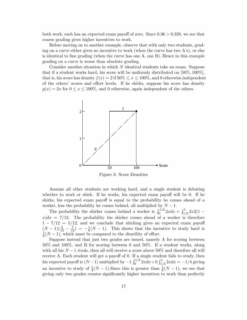
Consider another situation in which N identical students take an exam. Supposethat if a student works hard, his score will be uniformly distributed on [50%, 100%],that is, his score has density f(x) = 2 if 50% ≤ x ≤ 100%, and 0 otherwise,independentof the others’ scores and effort levels. If he shirks, suppose his score has densityg(x) = 2x for 0 ≤ x ≤ 100%, and 0 otherwise, again independent of the others.

1

0

2

50 100 Score

f

g

Figure 3: Score Densities

Assume all other students are working hard, and a single student is debatingwhether to work or shirk. If he works, his expected exam payoff will be 0. If heshirks, his expected exam payoff is equal to the probability he comes ahead of aworker, less the probability he comes behind, all multiplied by N − 1.

The probability the shirker comes behind a worker isR 1/20 2xdx +

R 11/2 2x2(1 −

x)dx = 7/12. The probability the shirker comes ahead of a worker is therefore1 − 7/12 = 5/12, and we conclude that shirking gives an expected exam payoff(N − 1)( 512 − 7

12) = −16(N − 1). This shows that the incentive to study hard is16(N − 1), which must be compared to the disutility of effort.Suppose instead that just two grades are issued, namely A for scoring between

50% and 100%, and B for scoring between 0 and 50%. If a student works, alongwith all his N − 1 rivals, then all will receive a score above 50% and therefore all willreceive A. Each student will get a payoff of 0. If a single student fails to study, thenhis expected payoff is (N−1) multiplied by −1 R 1/20 2xdx+0

R 11/2 2xdx = −1/4 giving

an incentive to study of 14(N − 1).Since this is greater than 16(N − 1), we see that

giving only two grades creates significantly higher incentives to work than perfectly

17

fine grading.We will show later that our partition of scores

P = {[0, 50%), [50%, 100%]}

into just two grades yields the optimal absolute grading partition.With three students the incentive to work under P is (1/4)(3 − 1) = 1/2. Now

consider grading on a curve. Giving everybody an A provides no incentive at all.Giving three grades is just like the perfectly fine partition with absolute gradingand is therefore not as good as the optimal partition ([0, 50), [50, 100)). (Indeed wecomputed that fine grading gave incentive 1/3). With a curve that gives two B’s andone A, the incentive to work is 99/324 < 1/2, while with a curve that gives one Band two A’s it is 63/324 < 1/2. Once again absolute grading is better than gradingon a curve.

As a third example, suppose an exam contains K questions, and that a studentwho studies has (independent) probability p of getting each question right, while ifhe shirks the probability drops to q < p. It will turn out that the optimal grading isperfectly fine.

As a final example, suppose that we are grading the relative performances of twohedge funds. Suppose that a hedge fund that works on research will generate logreturns normally distributed with mean μ and standard deviation σ, while a hedgefund that shirks will generate returns distributed according to μ < μ and σ > σ. Ifthe fund managers cared only about their relative grade, would they be motivated towork harder if the grade was simply their return? Intuitively that seems wrong, sincean extraordinarily high return is more likely from the high variance shirker, despitehis lower expected return. We shall see that the optimal grading scheme indeed doesnot reward higher returns after some point.

4.2 The General Theory with iid Students

We turn now to the general situation. Observe first that as long as the students areidentical, their expected exam scores must be zero if they all work, as we noted in theexamples. The incentive to work therefore is precisely the negative of the expected(exam) payoff to a shirker who competes against workers. It follows that there is nosimplification gained by assuming that each student’s performance is independent ofthe others’ effort levels. If in the second example we continued to let (f, g) be the scoredensities of the (workers, shirker), and introduced h 6= f as the score density whenall work, our analysis would remain absolutely unchanged; h would be irrelevant.

On the other hand, the following independence assumption does play an importantsimplifying role.

Assumption: Conditional on any choice of effort levels (e1, ..., en), students’ examscores are independent.

We shall maintain this assumption for the rest of the paper.

18

Our analysis of the optimal absolute grading partition begins by asking whetherthe shirker’s payoff can be lowered below zero by a single cut at θ, creating a twocell partition {(−∞, θ), [θ,∞)}. We shall find that if the worker’s score distributionf stochastically dominates the shirker’s score distribution g, then any cut will help,while under the reverse domination, every cut will hurt.

Next we consider a partition and ask whether cutting a cell in the partition intotwo cells will further help incentives or set them back. The answer depends on who isthe better player, conditional on both scores lying inside the same cell. If the shirkeris better, we must not reveal this, since we are trying to minimize his score, and keepthe cell uncut. For example, the shirker may be very unlikely to get a score above90. But conditional on both the shirker and worker getting above 90, it may be morelikely that the shirker does better. (The shirker may have memorized the answers tolast year’s exam. In the unlikely event that this year’s exam questions are the samehe will get 100; otherwise he will get 0.)

The guiding principle in creating optimal partitions is to mask regions of the scorespace where the shirker is better than the worker, and to ensure that across cells theworker is better, so that the partition reveals the deficiencies of the shirker. Thischaracterization will be used in Section 5 to prove that absolute grading is betterthan grading on a curve, and then again in Section 6 to derive the optimal wageschedule when workers are homogeneous.

Lemma 1: Suppose two students H and L take an exam, yielding independentscores xH and xL. If the grading partition is {(−∞, θ), [θ,∞)}, then the expectedexam payoff to L is

P (xL ∈ [θ,∞))− P (xH ∈ [θ,∞)).Similarly, if the grading partition includes cells [a, θ), [θ, b), for a < θ < b, thenconditional on both xH and xL being in [a, b), the expected exam payoff to L is

P (xL ∈ [θ, b))P (xL ∈ [a, b)) −

P (xH ∈ [θ, b))P (xH ∈ [a, b)) .

Proof: In the first case, the expected exam payoff to L is

P (xL ∈ [θ,∞) ∧ xH ∈ (−∞, θ))− P (xH ∈ [θ,∞) ∧ xL ∈ (−∞, θ)).

With independence, this becomes

P (xL ∈ [θ,∞))P (xH ∈ (−∞, θ))− P (xH ∈ [θ,∞))P (xL ∈ (−∞, θ))

= P (xL ∈ [θ,∞))(1− P (xH ∈ [θ,∞))− P (xH ∈ [θ,∞))(1− P (xL ∈ [θ,∞)))= P (xL ∈ [θ,∞))− P (xH ∈ [θ,∞)).

The second case is analogous. ¥

19

Corollary: If P is a partition of scores including the cell [a, b) and if P∗ modifiesP by cutting [a, b) at θ, into [a, θ) and [θ, b), leaving all the other cells intact, thenthe move from P to P∗ increases the expected exam payoff to L by

P (xL ∈ [a, b))P (xH ∈ [a, b))∙P (xL ∈ [θ, b)P (xL ∈ [a, b) −

P (xH ∈ [θ, b))P (xH ∈ [a, b))

¸.

Proof: This follows from Lemma 1 after observing that if either xL /∈ [a, b) orxH /∈ [a, b), the payoff is the same under P or P∗. ¥

This should remind the reader of stochastic dominance.

4.2.1 Stochastic Dominance

Definition: We say that the random variable x (stochastically) dominates the in-dependent random variable y on the interval [a, b) if, whenever P (x ∈ [a, b)) > 0 andP (y ∈ [a, b)) > 0, we have

P (x ∈ [θ, b)|x ∈ [a, b))− P (y ∈ [θ, b)|y ∈ [a, b)) ≥ 0,i.e.,

P (x ∈ [θ, b))P (x ∈ [a, b)) ≥

P (y ∈ [θ, b))P (y ∈ [a, b))

for all θ ∈ (a, b). In this case we writex % y on [a, b).

If the inequality is strict for all θ ∈ (a, b), we write x  y on [a, b) and call it strictdominance. If [a, b) = (−∞,∞), then we simply write x % y or x  y.

Stochastic dominance has an extremely important role to play in monotonic grad-ing schemes, including absolute grading.

Lemma 2: Suppose x % y. Let the exam scores x and y be independent of the examscores of every student n = 1, ..., N − 1. Let γ be any monotonic grading scheme forN students. Then the expected exam payoff to the last student N is at least as highunder an exam score of x as it is under y.

Proof: By independence, the payoffs from exam scores x and y depend only on theirdistributions. According to Theorem 1.A.1 of Shaked—Shanthikumar, there exist xand y with the same distributions as x and y respectively, such that x ≥ y withprobability one. But then for any realization of the other N − 1 scores, x will clearlyget a (weakly) higher payoff than y. ¥

It follows that if a shirker has exam scores distributed according to xL while theworker’s is distributed according to xH , and xL & xH , then no monotonic gradingscheme can provide any incentive to work. We might as well give all students an A.

20

In both our examples of this section, the worker scores stochastically dominatedthe shirker’s scores, and indeed this is what gave the student an incentive to workunder all the grading schemes.

It will be useful to also consider a strengthened form of domination.

Definition: We say that x uniformly dominates y on the interval [A,B) if x dom-inates y on every subinterval [a, b) ⊂ [A,B). In this case we write x %U y on [A,B).

Uniform domination can be characterized in terms of likelihood ratios in a mannerthat makes it much more handy to work with. But first we must restrict the randomvariables slightly.

Density Assumption: Whenever we consider several random variables (exam scores)together, either all will be discrete or else all will be continuous, i.e., have measurabledensity functions on (−∞,∞) with no atoms. In either case we can speak of thedensity f(t), for t ∈ (−∞,∞) or t ∈ {α1, α2, ..., αk} ⊂ (−∞,∞).

Lemma 3: Let x and y be independent on [A,B) with density functions f and g,respectively. Then x uniformly dominates y on [A,B) if and only if the likelihoodratio f(t)/g(t) is increasing almost everywhere on [A,B), where f(t)/g(t) can bedefined suitably arbitrarily if f(t) = g(t) = 0.

Proof: This follows from Theorem 1.C.2 in Shaked—Shanthikumar. ¥

It is critical in understanding the first two examples of this section to observethat although the worker’s scores (stochastically) dominates the shirker’s, there aresubintervals on which the shirker’s score uniformly (stochastically) dominates theworker’s. Thus in the first example, q/(2p(1−p)) = .8/.48 > .2/.16 = (1−q)/(1−p)2,so on the cell {0, 1} the shirker uniformly dominates the worker. In the secondexample of this section xL uniformly dominates xH on [50, 100].

Another instance of uniform domination occurs in the third example, where anexam has K independent questions, and a student has a probability p of getting anyanswer correct. If another student independently has probability q of getting eachquestion right, then the likelihood ratio condition reduces to21³

Kk

´pk(1− p)K−k³

Kk−1´pk−1(1− p)K−k+1

>

³Kk

´qk(1− q)K−k³

Kk−1´qk−1(1− q)K−k+1

21The notion of domination does not rely on independence. For example, suppose that withprobability π the two students have chance p1 > q1 of getting each question, while with probability1 − π they have chance p2 > q2 of getting each question; still the score of the first student woulduniformly dominate that of the second. This suggests that much of our analysis can be extended tononindependent scores, but we have not undertaken this extension here.

21

orp

1− p>

q

1− q.

Thus if p > q, the first score uniformly dominates the second score over the range ofall scores.

When f and g are differentiable, f(t)/g(t) is increasing if and only if f 0(t)/f(t) ≥g0(t)/g(t). Let N(μ, σ) denote the normal distribution with mean μ and standarddeviation σ. If x ∼ N(μ, σ) with density f(t) and y ∼ N(μ, σ) with density g(t) then

f 0(t)f(t)

=−(t− μ)

σ2;−(t− μ)

σ2=

g0(t)g(t)

∀t ∈ (−∞,∞).

If μ > μ and σ = σ, then x uniformly dominates y on all of (−∞,∞). More generally,x will uniformly dominate y on the interval including all t such that

t

σ2− t

σ2<

μ

σ2− μ

σ2

and y will uniformly dominate x on the complementary interval. Thus if σ2 < σ2,then x uniformly dominates y on the lower tail, and y uniformly dominates x on theupper tail. This is crucial in understanding the fourth example.22

Domination and uniform domination can be defined exactly the same way for anytotally ordered set, such as a partition P. The likelihood ratio criterion for uniformdomination appearing in Lemma 3 also carries over to partitions. Given a density fand a partition P, define the density

fP(x) =

(f(x) if {x} ∈ P1

b−aR ba f(t)dt if x ∈ [a, b) ∈ P

where the integral is understood to be a sum in the discrete case. The analogue ofLemma 3 still holds: x uniformly dominates y on [A,B) with respect to P if and onlyif fP(t)/gP(t) is increasing on [A,B).

4.2.2 Optimal Partitions

We are now ready to state some theorems about the optimal absolute grading parti-tion when students have conditionally independent scores. It turns out that uniformstochastic dominance plays the central role in determining whether there should bemasking (i.e., giving the same grade to different scores). If a worker’s score uniformlystochastically dominates a shirker’s, then the grading should be perfectly fine (so thatdoing better always means getting a strictly higher grade). Conversely, if on somesubinterval of scores [A,B) the shirker uniformly stochastically dominates the worker,then all scores in [A,B) should be given the same grade. When the score densities are

22The attentive reader might be puzzled, since the binomial exam scores “converge” to normal asK →∞, yet we never see the tail where xq dominates xp . That is because this tail is always beyondK. In fact it is not the exam scores, but normalized exam scores, which converge to normal, and themeans of xp and xq are diverging at the rate K (not

√K).

22

piecewise differentiable or discrete, (−∞,∞) can be divided into intervals over whichuniform stochastic dominance goes one way or the other, and so the optimal absolutepartition can be determined. The non-regular case is more subtle, and we have notcompletely characterized the optimal grading. But we give necessary conditions for apartition to be optimal and slightly stronger sufficient conditions for it to be optimal,based on whether the shirker score stochastically dominates the worker score insideeach partition cell, and whether the worker uniformly stochastically dominates theshirker score across (outside) partition cells.

The phrase “N iid students who can work or shirk” means that each student hastwo effort levels, and that assuming any one student shirks while the others work,he has score xL with density g while each other student k has an independent scorexk ∼ xH , with density f . (Here ∼ denotes identical in distribution.) We begin witha simple theorem showing that when xH &U xL, perfectly fine grading is optimal,even in the wider class of all monotonic and anonymous grading schemes.

Theorem 3 (Fine Grading Can Be Optimal): Let there be N iid students whocan work or shirk. Suppose xH &U xL. Further, suppose xH and xL are eitherdiscrete or have piecewise continuous densities f and g with no atoms. Then finegrading is optimal in the class of all monotonic, anonymous grading schemes.

Proof: Consider the case of two students, a worker and a shirker. A monotonicgrading scheme γ differs from fine precisely on the set

W = {(xL, xH) ∈ R2 : xL 6= xH , yet γ gives xL and xH the same grade}.

Suppose first that the densities f and g are discrete. By anonymity, (α, β) ∈ W ifand only if (β, α) ∈W . But from the uniform domination xH &U xL, we know thatif β > α, then f(β)/g(β) ≥ f(α)/g(α). Hence replacing the masking grading γ onW with fine grading lowers the expected exam payoff to the shirker byX

(α,β)∈Wα<β

[f(β)g(α)− g(β)f(α)] ≥ 0.

Next suppose that f and g are piecewise continuous. SinceW is measurable it canbe approximated arbitrarily closely (in Lebesgue measure) by a union of small squaresQ = {(xL, xH) : α− ε ≤ xL < α+ ε and β − ε ≤ xH < β + ε} whose interiors do notcontain any points of discontinuity of f and g. By anonymity, we may assume that themirror squareQ∗ = {(xL, xH) : β−ε ≤ xL < β+ε and α−ε ≤ xH < α+ε} is also partof the approximation. These squares have area approximately equal to ε2f(α)g(β) orε2g(α)f(β). If β > α, then by uniform stochastic dominance, f(β)g(α) ≥ g(β)f(α).The masking on W thus hides the fact that xH would have come ahead of xL moreoften than behind xL when both variables are in W . Hence masking W does notimprove the incentive to work. A similar argument could be given with more thantwo students. ¥

23

Now we focus on absolute grading, giving conditions under which a cell [a, b)should not be cut by any optimal partition.

Theorem 4 (Coarseness in the Optimal Grading): Let there be N iid studentswho can work or shirk. Suppose that on some interval [a, b), xL uniformly dominatesxH . Then for any partition P that cuts [a, b), there is another partition P∗ that givesat least as much incentive to work without cutting [a, b). If xL strictly uniformlydominates xH on [a, b), then every optimal grading partition is coarse on [a, b).

Proof: Consider the following picture:

βα a θ b

Figure 4: Cutting (a, b) at θ

Let P be a partition that cuts [a, b) just once, that is, suppose that θ ∈ (a, b),and that [α, θ) ∈ P and [θ, β) ∈ P, where α ≤ a < θ < b ≤ β, where −α orβ might be infinite. (The cases where the closed end comes on the right insteadof the left are handled the same way.) For the rest of the proof all probabilitieswill be taken conditional on xL and xH being in [α, β]. For ease of notation, wesuppress this conditionality. Thus when we write P (xL ∈ [a, b)), we really meanP (xL ∈ [a, b))/P (xL ∈ [α, β)), etc.

>From the Corollary to Lemma 1, we know that the expected payoff to L in P(conditional on both xL and xH in [α, β)) is

P (xL ∈ [θ, β))− P (xH ∈ [θ, β)).

Suppose first that P (xL ∈ [θ, b)) ≥ P (xH ∈ [θ, b)). Then

P (xL ∈ [b, β))− P (xH ∈ [b, β))≤ P (xL ∈ [θ, β))− P (xH ∈ [θ, β)).

It follows from the Corollary to Lemma 1 that the partition obtained from P bymoving the cut from θ to b (i.e., by replacing [α, θ) and [θ, β) with [α, b) and [b, β))weakly lowers the expected exam payoff to L, without cutting [a, b), as was to beproved.

Suppose on the other hand that P (xL ∈ [θ, b)) < P (xH ∈ [θ, b)). From thedominance of xL over xH on [a, b), we conclude that P (xL ∈ [a, θ)) < P (xH ∈ [a, θ)).It follows immediately that

P (xL ∈ [a, β))− P (xH ∈ [a, β))< P (xL ∈ [θ, β))− P (xH ∈ [θ, β))

24

showing that the partition obtained from P by moving the cut from θ to a (i.e.,by replacing [α, θ) and [θ, β) with [α, a) and [a, β)) lowers the expected payoff to L,without cutting [a, b], as was to be shown.

It only remains to consider the case where P cuts (a, b) multiple times. If thereare a finite number of cuts, that case can be reduced to the case where (a, b) is cutonce, by arbitrarily choosing any cut θ ∈ (a, b), and then choosing the highest cutc < θ and the lowest cut d > θ, and replacing (a, b) with (a, b)∩(c, d). By the uniformdominance of xL over xH on [a, b), xL dominates xH on [a, b)∩ [c, d). The same proofcan then be repeated. This reduces the number of cuts by 1. The reduction can thenbe iterated.

Finally, suppose there is a subinterval [c, d) ⊂ [a, b) on which P is perfectly fine.Change P to P∗ by completely masking [c, d). Since xL dominates xH on [c, d), thismasking can only (weakly) lower the expected exam payoff to L. In this way wereduce the problem to finitely many cuts. This proves the first claim of the theorem.The second claim is proved the same way. ¥

Theorem 4 shows that if work leads to a normal distribution N(μ, σ) of scores,and shirk leads to N(μ, σ), where σ 6= σ, then one tail of scores will be completelymasked in any optimal partition.

Theorem 4 also leads to a sufficient condition for the optimality of a partitionP. We say that xL uniformly dominates xH inside a partition P if xL &U xH insideevery cell [a, b) ∈ P. We say that xH uniformly dominates xL outside a partition Pif xH &U xL on P, i.e., across the cells of P.

Theorem 5 (Uniform Inside and Outside Domination Implies Optimality):Let there be N iid students who can work or shirk. Let P be a partition such that forevery cell [a, b) ∈ P, xL %U xH on [a, b), and such that xH %U xL on the partitionP. Then P is optimal.

Proof: Suppose P 0 does better than P. From Theorem 4, we know that there isP 00 that does at least as well as P 0, and which does not cut any cell in P. But everycell in P 00 is refined by cells in P. Since xH %U xL on P, it follows that the payoff toxL is weakly lower in P than in P 00, a contradiction. ¥

Suppose that all students are homogeneous, with independent, and normally dis-tributed exam scores. If work raises a student’s expected exam score, without chang-ing its variance, then Theorem 5 implies that an optimal grading scheme is to postthe exact scores.

Similarly, if the K exam questions are identical, independent trials, and if hardwork allows a student to raise his probability of getting each answer right, then againan optimal grading scheme is to reveal the exact scores.

But consider the two leading examples of this section. There we found that givingjust two grades, A and B, improved incentives beyond what could be achieved byfully revealing the scores. Theorem 5 and Lemma 3 guarantee that these are indeed

25

optimal partitions. In the first example, xL uniformly dominates xH on {0, 1}, whilexH uniformly dominates xL across the partition cells {0, 1}, {2}, since .36/.64 > 0/1.In the second example, inside the cell [0, 50), xH has probability zero, so xL triviallyuniformly dominates it. Inside the other cell [50, 100), f(t)/g(t) = 2/2t = 1/t isstrictly falling, so xL uniformly dominates xH . Across cells we can check that xHuniformly dominates xL. On [0, 50), we can define the effective density of a workeras fP(t) = 0, and that of a shirker as gP(t) = .5. On [50, 100) the effective densitiesbecome fP(t) = 2 and gP(t) = 1.5. Clearly fP(t)/gP(t) is increasing.

In our next theorem we describe necessary conditions for a partition to be optimal,when agents are homogeneous. The “outside” condition, that xH %U xL on P, is thesame as the sufficient “outside” condition appearing in Theorem 5. But the “inside”condition xL % xH on each cell [a, b) in P is weaker than the sufficient “inside”condition xL %U xH appearing in Theorem 5. For the theorem we need to imposeslightly stronger conditions.

Definition: The exam performances xL and xH , with densities f and g, are calledgeneric iff f and g are both discrete or both continuous, and there is a countable set{· · · < ai < ai+1 < · · · } such that f(t)/g(t) is strictly increasing on [ai, ai+1) for alleven i and strictly decreasing for all odd i.

Theorem 6 (Optimality Implies Domination): Let there be N iid students whocan work or shirk. Let P be an optimal absolute grading partition. Then for any cell[a, b) ∈ P, xL % xH on [a, b). Furthermore, if exam performances are all discrete,or all have piecewise differentiable densities, or are generic, then xH %U xL on thetotally ordered set P.

Proof: Consider any cell [a, b) in P such that P (xL ∈ [a, b))P (xH ∈ [a, b)) > 0.Suppose there is some θ ∈ [a, b) with

P (xL ∈ [θ, b))P (xL ∈ [a, b)) −

P (xH ∈ [θ, b))P (xH ∈ [a, b)) < 0.

Change P to P∗ by replacing [a, b) with [a, θ) and [θ, b). By the Corollary to Lemma1, this must lower the expected exam payoff to the shirker against each worker. Butthis means that P∗ is a better partition than P, a contradiction proving that xL % xHon [a, b).

Consider two consecutive cells [a, b) and [b, c) in P whose union (a, b] ∪ (b, c] haspositive probability of being reached by both xL and xH . Then it is clear from theCorollary to Lemma 1 that

P (xH ∈ [b, c))P (xH ∈ [a, c)) ≥

P (xL ∈ [b, c))P (xL ∈ [a, c)) ,

otherwise the partition P∗ obtained from P by replacing the two cells [a, b) and [b, c)with the single cell [a, c) would lower the expected exam score to L, contradicting

26

the optimality of P. Hence the likelihood ratio property holds for fP and gP acrossconsecutive masked intervals. This same logic applies when exam scores are discrete.

The partition P must consist of intervals, each of which is fine or masked. IffP(x)/gP(x) is increasing, then by Lemma 3 we have that x &U y on P. Supposeto the contrary that there is α < β with fP(α)/gP(α) > fP(β)/gP(β). Then we canassume that either (1) α and β are in the same fine interval, or (2) α is in a fineinterval and β is in the next (coarse) interval, or the reverse (3).

Suppose α and β are in the same fine interval. If the exam scores are generic,then on some open interval (a, b) ⊂ (α, β), f(t)/g(t) is strictly decreasing, hence (byTheorem 4) (a, b) should be masked, contradicting the optimality of P. If f and gare piecewise differentiable, and there is a point θ ∈ (α, β) of differentiability with(d/dt)(f(θ)/g(θ)) < 0, then on some small interval (a, b), with θ ∈ (a, b) ⊂ (α, β),f(t)/g(t) is strictly decreasing, again contradicting Theorem 4. Otherwise there mustbe a jump down of f/g at a nondifferentiable point θ ∈ (α, β).

Nearby, f(t)/g(t) > M > m > f(s)/g(s) for all a < t < θ < s < b. Modify P bymasking the interval [θ − ε, θ + ε) ⊂ [a, b). We claim that this will lower the payoffto xL, contradicting the optimality of P. Conditional on both xH and xL fallinginto [θ − ε, θ + ε), P{xL ∈ (θ, θ + ε) and xH ∈ [θ − ε, θ)} − P{xH ∈ (θ, θ + ε) andxL ∈ [θ−ε, θ)} > K > 0, independent of ε. But conditional on both xL and xH lyingin (θ, θ+ ε), or both lying in [θ− ε, θ), the probability of xL coming ahead minus theprobability of xH coming ahead converges to 0 as ε → 0, because of the continuityof f and g on [θ− ε, θ). Thus perfectly fine grading on [θ − ε, θ + ε) gives L an edgethat should have been eliminated by masking.

It only remains to consider the case where the drop in fP(x)/gP(x) occurs at θbecause θ is the cut between a perfectly fine cell [c, θ) of P and a masked cell [θ, d)of P (or vice versa). We argue that P could not be optimal, because moving the cutfrom θ to θ − ε would lower the payoff to xL. We rely on the continuity of f to theleft of θ, which holds for the generic case or the piecewise differentiable case.

Indeed, the change in expected payoff to L from moving the cut to θ − ε is

P (xH ∈ [θ, b))P (θ − ε ≤ xL < θ)− P (xL ∈ [θ, b))P (θ − ε ≤ xH < θ)

+ P (θ − ε ≤ xH < θ)P (θ − ε ≤ xL < θ)[P (xH > xL|θ − ε ≤ xL, xH < θ)

− P (xL > xH |θ − ε ≤ xL, xH < θ)].

Observe that the third term goes to zero as ε2 when ε→ 0, whereas the first twoterms are of the order of ε. As ε → 0, P (θ − ε ≤ xH < θ) converges to εf(θ), andP (θ − ε ≤ xL < θ) converges to εg(θ). Thus if f(θ−)/g(θ−) > fP(θ+)/gP(θ+), thenthe first two terms add to less than zero. This shows that the extra masking obtainedby lowering the cut θ to θ − ε reduces the expected exam payoff to L, contradictingthe optimality of P. ¥

We can use Theorems 4 and 6 to completely characterize the optimal partitions forthe normally distributed case, and more generally, for the generic case, even thoughTheorem 5 cannot be applied. Consider again the situation where f ∼ N(μ, σ) andg ∼ N(μ, σ) with σ < σ. We have seen that the function f(t)/g(t) is differentiable and

27

single-peaked, strictly rising for −∞ < t ≤ x and strictly falling for x ≤ t <∞. SeeFigure 5. Thus the normal case is differentiable and generic. We know from Theorem4 that any partition that cuts (x,∞) can be strictly improved by a partition thatleaves (x,∞) uncut.

maskedperfectly fine

( )

( )

f x

g x

−∞ ∞Ax x

Figure 5: Normally Distributed: μ > μ, σ > σ

Moreover, since f(t)/g(t) is strictly increasing on (−∞, x), we know from Theorem6 that if there is any cut in (−∞, x), say at xA, then (−∞, xA) should be perfectlyfine. It follows that the optimal partition must be of the form {(−∞, xA), [xA,∞)}with (−∞, xA) perfectly fine and [xA,∞) completely masked, and xA < x. The pointxA is uniquely defined by the greatest x ≤ x such that

f(xA)

g(xA)=

P (xH ≥ xA)

P (xL ≥ xA).

At x = x, f(x)/g(x) > P (xH ≥ x)/P (xL ≥ x). As x falls to the left of x, f(x)/g(x)also falls, but P (xH ≥ x)/P (xL ≥ x) rises as long as f(x)/g(x) > P (xH ≥ x)/P (xL ≥x). Since f(x)/g(x) > 1 and limx→−∞ f(x)/g(x) = 0, xA exists.

If x > xA, then the partition {(−∞, x), [x,∞)} violates the outside condition ofTheorem 6, while if x < xA it violates the inside condition on the cell [x,∞), as seenby cutting this cell at xA.

The general picture is as follows

Theorem 7 (Optimal Partitions for Generic Densities): Consider the case ofgeneric densities f and g. In any optimal partition P, all the cuts are in the risingsegments (ai, ai+1) of f/g, where i is even. If there is a cut in (ai, ai+1), then theset of all cuts in (ai, ai+1) is a fine interval [αi, βi) ⊂ (ai, ai+1) in P , or else a pointαi = βi. In either case,

f(βi)

g(βi)=

R yβif(t)dtR y

βig(t)dt

where y is the smallest cut to the right of βi, and

f(αi)

g(αi)=

R αix f(t)dtR αix g(t)dt

where x is the biggest cut to the left of αi. Thus the optimal partition has at mostone more cell than the number of extremal points of f/g.

28

Proof: Immediate from Theorems 4 and 6, and Lemma 3, using the same logic asin Figure 5. ¥

masked

−∞ ∞AxCx 1a 2a

fine fine

Bx 3a

masked

( )

( )

f x

g x

Figure 6: Generic Regular Densities

5 Grading on a Curve

We have assumed that students care only about their relative grade. It would seemtherefore that relative grading, i.e., grading on a curve, would provide the best in-centives. But in fact the contrary is true. We shall prove that when all the studentsare disparate or homogeneous, it is always better to grade according to an absolutescale, no matter how many students are in the class.

With a large number of students of each type, there is practically no differencebetween grading on a curve and absolute grading. Giving an A to top 10% of studentscan be replicated with very high probability by giving an A to all scores above xA,for some appropriate threshold xA.

5.1 Disparate Students

Let there be Ni students of type i = 1, ..., , as in Section 3.3. Grading on a curvemeans specifying integers K = (KA,KB, ...,KZ) with KA +KB + · · ·+KZ = N =N + · · ·+N1, where the top KA student exam scores get A, the next KB get B andso on. (The probability of ties is zero.)

If there is only one disparate student of each type, then the student of type i willscore below − i students and above i−1 students whether he works or shirks. Withgrading on a curve, his letter grade must therefore be independent of his effort, andso grading on a curve provides no work incentive whatsoever.

Consider a general population N = (N1, ..., N ), and any grading on a curveK = (KA,KB, ...,KZ). We can find an absolute grading scheme that creates thesame incentives to work for types 2, ..., , and at least as much for type 1.

29

Let μi measure the distribution of scores of a type i agent when he works (soμi(T ) = Prob(xHi ∈ T ) for every T ⊂ R). Define μ ≡ Pi=1Niμi. For any relativegrade α, cut R at the minimum point x such that

KA + · · ·+Kα = μ[x,∞).

It is easy to check that the absolute partition defined by these cuts does the job.

5.2 Homogeneous Students

Theorem 8 (Absolute Grading Beats Grading on a Curve): Let there beN iid students who can work or shirk. Let all their score densities be piecewisedifferentiable. Let P be an optimal absolute grading partition. Then P gives at leastas much incentive for work as any grading on a curve.

The proof relies on the inside and outside domination criteria for any optimalpartition given in Theorem 6. Starting from an optimal partition, we prove thestronger result that conditional on the number of students who get each absolutegrade, no grading on a curve will do better.

For the proof we first establish a simple lemma.

Lemma 4: Denote scores in [θ,∞) as A. Suppose N − 1 students work hard, andeach has probability p of getting an A, while one student shirks and has probabilityq < p of getting an A. Suppose all scores are independent. If exactly K students windup with A, the conditional probability that the shirker got A is less than K/N , whilethe probability any hard worker got A is more than K/N .

Proof: The conditional probability the shirker got A is

q

µN − 1K − 1

¶pK−1(1− p)N−K

q

µN − 1K − 1

¶pK−1(1− p)N−K + (1− q)

µN − 1K

¶pK(1− p)N−K−1

which is strictly monotonically increasing in q (as can easily be seen by dividingnumerator and denominator by the numerator). But when q = p, symmetry impliesthat the expression must be exactly K/N . Hence the probability the shirker got A isless thanK/N . Since exactly the proportion K/N students did get A, the probabilityof the good students getting A must then be more than K/N . ¥

Proof of Theorem 8: Let Q be any partition of class rank {1, 2, ..., |N |}, repre-senting an arbitrary grading on a curve.

For any possible exam scores x = (xn)n∈N , and any absolute interval G in P(whether coarse or fine), let μG(x) be the number of exam scores lying in G. For anycurved grade γ, let μγG(x) be the number of scores in G that also get curved grade

30

γ. Note that since there are no ties, (μγG)G∈P can be deduced from μ ≡ (μG)G∈P . Apicture helps to clarify the situation.

δ γ β α

ABC

Figure 7. Absolute vs. Relative Grading

In the picture there are 4 A’s, 3 B’s, and 3 C’s on the absolute scale. The relativescale gives grade α to the top score, β to scores 2 and 3, γ to {4, 5, 6, 7, 8, 9}, and δto the 10th highest score. We can deduce that μγA = 1, μ

γB = 3, and μγC = 2.

Define the join P∨Q of P and Q as follows: given scores (xn)n∈N , the exam gradefor xn is strictly higher according to P ∨Q than the exam grade for xm iff either theabsolute letter grade for xn is strictly higher than for xm, or the relative grade forxn is strictly higher than for xm. Conditional on μ, that is achieved by cutting thecurved grade cell γ into three curved grades γA, γB, and γC with cardinalities 1, 3,and 2, respectively.

We will now argue that if we grade according to the join P ∨Q then the expectedexam payoff of the shirker is no more than it was in Q. If a relative grade, such as γin Q, is refined in P ∨Q, we show that the expected score of the shirker, conditionalon μ and on his being in γ to begin with, will not go up. Since splitting γ does notaffect scores against students outside γ, it suffices to show that the expected examscore of the shirker against the other students in γ must be at most zero.

Let μ be an arbitrary interval distribution of scores such that μG ≤ 1 for every fineinterval G in P. By subdividing fine intervals into smaller and smaller fine intervals,the probability that two scores fall in a single fine interval goes to zero, so we canrestrict attention to such μ.

Let γ be any curved grade with P (xL ∈ γ|μ) > 0. Let P∗ be the collection ofintervals G in P such that μγG ≥ 1. Clearly P∗ has a finite number of elements.

Let q be the probabilities of a shirker getting each absolute grade, conditional onthe grade distribution μ and the shirker being in γ.

We shall show that if C < B are intervals in P∗ with qB > 0, then qC > 0 and

qBqC≤ μγB

μγC.

Suppose γ includes the top μγC ≤ μC scores in C. If C is fine, then by hypothesisμγC = μC = 1, and P (xL ∈ C ∩ γ|μ & xL ∈ C) = 1. If the interval C is masked, thenby Theorem 6 the shirker dominates inside the cell, hence in either case

P (xL ∈ C ∩ γ|μ & xL ∈ C) ≥ μγCμC

.

31

By Bayes Law,

qC = P (xL ∈ C|μ & xL ∈ γ)

= P (xL ∈ C ∩ γ|μ & xL ∈ C)P (xL ∈ C|μ)/P (xL ∈ γ|μ).

Thus

qC ≥ μγCμC

P (xL ∈ C|μ)P (xL ∈ γ|μ) .

Similarly, if only the bottom part of scores in B are included in γ, then

P (xL ∈ B ∩ γ|μ & xL ∈ B) ≤ μγBμB

.

Thus arguing as with C,

qB ≤ μγBμB

P (xL ∈ B|μ)P (xL ∈ γ|μ) .

If qB > 0, then P (xL ∈ B|μ) > 0, and by Lemma 4,P (xL ∈ B|μ)P (xL ∈ C|μ) ≤

μBμC

.

Hence P (xL ∈ C|μ) > 0. ThereforeqBqC≤ μγBP (xL ∈ B|μ)

μBP (xL ∈ C|μ)μCμγC≤ μγB

μγC,

as claimed.It follows that the shirker’s expected exam payoff according to P ∨Q against the

otherP

G∈P∗ μγG − 1 scores in μ must be non-positive. Thus, conditional on μ alone,

the expected exam payoff of a shirker is lower when grading by P ∨ Q than whengrading by Q.

Thus we have shown that the expected exam payoff to a shirker is lower underP ∨Q than under Q.

To conclude the proof, we need only show that the expected exam payoff of theshirker in P is even lower (weakly) than his expected exam payoff in P ∨ Q. Thisfollows at once from the fact (see Theorem 2) that conditional on being in a maskedcell of P, the score of the shirker dominates the score of a worker. But then, byLemma 2, any monotonic grading scheme within cells of P (as is induced by P ∨Q)will weakly increase the payoff of the shirker. ¥

6 Games of Money and Status: Setting Optimal WageSchedules

Suppose now that the agents are workers in a firm who obtain direct utility from thepurchasing power of wages and status utility from higher wages.

32

In keeping with our focus on ordinal status, we assume that if the N workers arepaid wages w = (w1, ..., wN), they obtain utility

un(w) = wn +#{j : wn > wj}−#{j : wj > wn}.The employer seeks to minimize his total wage bill, subject to providing incentives

to work of at least dn, for each worker n. The wage schedule he sets must be ananonymous and monotonic function of outputs.

As before, wages can be awarded on the basis of absolute performance or relativeperformance (analogous to grading on a curve). If the status payoff were eliminated,leaving behind only utility for money, then paying relative wages would resemble atournament with multiple prizes: one can think of different players who are awardedthe same prize as receiving the same grade.23

With status, we shall focus instead on wage schedules that are based on absoluteperformance, paying each worker according to his own output.24 We conjecture that,as with games of pure status, absolute wages are better for the employer than relativewages anyway. (In the case of disparate workers, this is obvious from Section 5.1.)

Our model is thus the same as the classical wage problem, except that we haveattached status to wages (and assumed participation constraints are not binding).

6.1 Disparate Workers

First consider the disparate case with Ni ≥ 1 workers of type i = 1, ..., , exactly asin Section 3, with exam scores reinterpreted as output produced. (Thus if a workerof type i shirks, he still produces more output than any worker of type i − 1.) Wesaw there that the principal could provide the greatest status incentives to work byclumping outputs into +1 grades. Now we ask the question: given that the principalcan use both status and wages as motivators, should he use them in equal proportionfor all workers? Or should he, for example, reserve status mostly for higher workertypes?

Since workers are disparate, strictly monotonic wages (such as piece-rate con-tracts) are suboptimal, because they squander the motivating power of status. Ex-actly as in Section 3, it will be optimal to set + 1 different grade wages, with theupper (pi)-fraction of i’s outputs assigned wage wi and the lower (1 − pi)-fractionassigned wage wi−1 for 1 ≤ i ≤ , where w0 = 0. (In order to signal that grade iconfers higher status than grade i−1, the principal will need to assign wi > wi−1. Toguarantee compactness, we allow him the freedom to set wi = wi−1 and still createa difference in status, e.g., via a title.25 It will turn out that under the conditions ofTheorem 9, he will never exercise this freedom.)23 In much of the tournament literature, the focus is on a single prize (see, e.g., Lazear—Rosen

[1981] and Green—Stokey [1983]). Even when multiple prizes are allowed for, it is optimal to handout only one (see Moldovanu—Sela [2001]). We reach a different conclusion because, in contrast totournaments, the status of coming ahead is not merely instrumental in getting a bigger prize but isvalued in and of itself.24The focus of Moldovanu—Sela—Shi (2005) is on relative wages.25We could have postulated instead that wi confers higher status than wj if, and only if, wi ≥ wj+δ

for some threshold δ > 0. Then our last constraint in the principal’s optimization problem would

33

The employer’s optimization problem is given below. One critical aspect of theproblem is that we have capped the maximum wage at an arbitrary, but high, levelM . The employer seeks to minimize his wage bill, subject to incentivizing everyoneto work:

minp,w

Xi=1

[(1− pi)wi−1 + piwi]Ni = minp,w

(Xi=1

wi−1Ni +Xi=1

pi(wi −wi−1)Ni

)s.t. I1 ≡ p1[(N1 − 1) + (1− p2)N2] + p1(w1 −w0) ≥ d1

...

Ii ≡ pi[(Ni − 1) + (1− pi+1)Ni+1 + pi−1Ni−1] + pi(wi −wi−1) ≥ di, for 1 < i <...

I ≡ p [(N − 1) + p −1N −1] + p (w −w −1) ≥ d

0 ≤ pi ≤ 10 = w0 ≤ w1 ≤ · · · ≤ w ≤M

Note that each agent i’s incentive Ii consists of the old (from Section 3.3) statusincentive Ii plus a wage incentive pi(wi−wi−1). We assume that the capM >

Pi=1 di.

If there were no status attached to higher wages, the employer would simply payeach worker type its disutility of effort, setting pi = 1 and wi − wi−1 = di for alli = 1, ..., . Wages would never rise faster than disutilities as the ability i increased.But Theorem 9 shows that when wages confer status, it is uniquely optimal (nomatter what the population distribution N1, ...,N ) to pay an astronomical wage to atiny number of top performers. The shape of the wage schedule for the other workersdepends on N1, ..., N , as well as d1, ..., d , and will be described in Section 6.1.1.

Theorem 9 (Elite Performers Get Exorbitant Wages): Let there be dis-parate types of workers, with Ni ≥ 1 of each type i = 1, ..., . Suppose their disutilities(d1, ..., d ) of work are such that at any feasible wage schedule (p, w) they each get awage incentive (in addition to their status incentive),26 i.e., pi(wi − wi−1) > 0 foreach i = 1, ..., .

Then there is a unique optimal status partition and wage schedule (p,w). In factpi = 1 for all i = 1, ..., − 1, so that any two workers of the same type below getthe same status and wage. But p ≤Pi=1 di/M , and w = M . In other words, forlarge M , a tiny elite p N out of the highest type is paid the exorbitant salary M ,while the rest of their type obtain the same status and pay as type − 1.

Proof: It will be useful to keep in mind throughout that raising pi has the effect ofraising Ii and Ii+1 and lowering Ii−1 without disturbing other incentives. Similarly,

read: 0 = w0, wi + δ ≤ wi+1 for 1 ≤ i ≤ − 1, w ≤ M . It is worth noting that as d → ∞,pi(wi − wi−1)→∞ since the status incentive terms Ii(p) are bounded by N1 + · · ·+N . Thus theconstraints wi + δ ≤ wi+1 are automatically satisfied for large enough d (given any δ).26This is guaranteed if, for example, Ni−1+Ni+Ni+1 < di for all i (with N0 = N +1 = 0). Would

anybody work for free, just for the status of coming ahead of all his peers?

34

raising wi raises Ii and lowers Ii+1, with no other effect.Raising p1 improves the status incentive for agents of type 1 and 2, without

disturbing the incentives of the others, allowing the employer to reduce w1. Thusp1 = 1.

Inductively assume that p1 = · · · = pi−1 = 1 for i < . Suppose pi < 1.Set wi−1 = wi−1 + εNi and pi = pi + ε. Then the status incentive of i − 1 goes

down by εNipi−1 = εNi, but his wage incentive goes up by the same amount: sincepi−1 = 1, pi−1(wi−1 −wi−2) = pi−1(wi−1 −wi−2) + εNi.

Also, the status incentive of i goes up by

∆Ii(ε) ≡ ε[(Ni − 1) + (1− pi+1)Ni+1 +Ni−1].

This allows us to reduce his wage incentive by the same amount. So, set wi to satisfy

pi(wi − wi−1) ≡ pi(wi −wi−1)−∆Ii(ε).For small ε, ∆Ii(ε) is small, so pi(wi − wi−1) > 0 implies that pi(wi − wi−1) > 0,which in turn implies wi > wi−1, retaining the monotonicity of the revised wages.We shall be assuming ε small enough to guarantee monotonicity in all future wagerevisions, without explicitly saying so.

Note that

wi =pipiwi + wi−1 − pi

piwi−1 − 1

pi∆Ii(ε)

=pi

pi + εwi +

µ1− pi

pi + ε

¶wi−1 + εNi − 1

pi + ε∆Ii(ε)

< wi + εNi − ε[(Ni − 1) + (1− pi+1)Ni+1 +Ni−1]≤ wi − ε(Ni−1 − 1) ≤ wi

since wi > wi−1 and pi + ε < 1 (if pi < 1 and ε is small) and Ni−1 ≥ 1.Finally, the status incentive of i+ 1 goes up by

∆Ii+1(ε) ≡ εpi+1Ni.

Therefore the wage incentive of i + 1 can be reduced by the same amount. So setwi+1 to satisfy

pi+1(wi+1 − wi) = pi+1(wi+1 −wi)−∆Ii+1(ε).Since wi < wi, clearly wi+1 < wi+1. Hence recursively setting

wj − wj−1 = wj −wj−1 for j > i+ 1

further lowers wages without changing incentives.It only remains to show that the wage bill defined in the employer minimization

problem has gone down. The only terms that increase are

wi−1Ni and pi−1(wi−1 −wi−2)Ni−1

35

while many terms are reduced, including

pi(wi −wi−1)Ni and pi+1(wi+1 −wi)Ni+1.

The increases add up toεNiNi + εNiNi−1,

while just these two reductions add to

∆Ii(ε)Ni +∆Ii+1(ε)Ni+1

= εNi[(Ni − 1) + (1− pi+1)Ni+1 +Ni−1] + εpi+1NiNi+1

= εN2i + εNiNi−1 + εNi(Ni+1 − 1).

Since Ni+1 ≥ 1, the reduction is at least as big as the increase. But we have ignoredmany other strictly positive reductions (for example in wi+1Ni+1). This contradictionproves that pi = 1, for i = 2, ..., − 1.

Now suppose w < M . Since p (w − w −1) > 0, clearly p > 0. Lower p by ε.This raises the status incentive of type −1 workers by εN , enabling us to lower thewage incentive for type − 1 by the same amount.

Recalling that p −1 = 1, set w −1 to satisfy

(w −1 −w −2) = (w −1 −w −2)− εN .

This drop in p unfortunately lowers the status incentive of type by ε(N − 1 +N −1). Therefore we must raise the wage incentive of , choosing w to solve

(p − ε)(w − w −1) = p (w −w −1) + ε(N −1 +N − 1).Fortunately, there is no group + 1 to be affected by the change in p , which is whyit will turn out to be optimal to lower p as long as w < M , whereas it was shownto be optimal to raise pi all the way to 1 for any i < .

Indeed the terms in the wage bill that change are

w −1N + p −1(w −1 −w −2)N −1 + p (w −w −1)N .

The net change in those terms is

−εN2 − εN N −1 + ε(N −1 +N − 1)N= −εN < 0

showing that the wage bill can be reduced, a contradiction. This proves that w =M .Clearly, for any 1 ≤ i ≤ − 2, the wage incentive

wi −wi−1 = pi(wi −wi−1) = di − Ii = di − (Ni +Ni−1 − 1).This recursively proves that wi is uniquely determined (starting from w0 = 0), fori = 1, ..., − 2. Also

w −1 −w −2 = d −1 − [N −2 +N −1 + (1− p )N − 1]

36

and

M −w −1 =d

p− [N −1 +N − 1]

(recalling that w ≡ M in the last equation). It can be checked27 that there is aunique solution w −1, p of these two simultaneous equations, so that the optimalwage schedule is determined uniquely.

Summing the inequalities wi −wi−1 ≤ di over i = 1, ..., − 1 gives

w −1 ≤ d1 + · · ·+ d −1.

Since the wage incentive of is at most d , we have

p (M −w −1) ≤ d ,

hence

p ≤ d + p w −1M

≤ d +w −1M

≤P

i=1 diM

. ¥

Theorem 9 shows that when workers are disparate, the interplay of status incen-tives and wage incentives produces an optimal hierarchy that is substantially differentfrom what was generated in the game of pure status discussed in Section 3. In thepure status case, it was essential that workers of the same type could end up withdifferent status, so we found pi < 1 for all 2 ≤ i ≤ . The opportunity to motivateworkers via money ensures that only the top group should be split into differentstatus groups, so now pi = 1 for 1 ≤ i ≤ − 1.

Theorem 9 also gives an explanation via status for the exorbitant pay often seen atthe very top of some real world hierarchies. It is cheaper to incentivize the managingdirectors of type − 1 as much as possible via status rather than wages. To achievethis they must be able to get the same status as most of the senior managing directorsof type , if they work hard. This fixes the wage of the latter group at the managingdirector’s level. In order to incentivize the senior managing directors, they are givento understand that the CEO will be chosen from among their rank, and even thoughthe chance of getting selected is small, the salary is huge.

This stratagem of paying a huge salary to the tiny fraction of top performers ina group is counterproductive at any level below , because monotonicity would forcethe employer to pay all workers of higher type at least as much.

6.1.1 Wage Differentials for Disparate Workers

The conclusions about exorbitant pay for the CEO and pi = 1 for all i = 1, ..., − 1are quite robust; they hold regardless of the distribution of abilities N1, ...,N , or thedisutilities of work d1, ..., d .

But the wage differentials wi − wi−1 for i < do depend on the Nj ’s and dj’s.Our analysis is based on the following corollary:

27Adding the two equations yields a quadratic in the single unknown p . This quadratic is convexand has a negative value at p = 0 and therefore a unique positive solution.

37

Corollary to Theorem 9: Under the conditions of Theorem 9, I1 = N1 − 1 <I2 = N1+N2− 1; Ii = Ni−1+Ni−1 for i = 3, ..., − 2. Also, I −1 = N −2+N −1+(1− p )N − 1 ≈ N −2 +N −1 +N − 1. Finally, I = p (N −1 +N − 1) ≈ 0.

Thus for 2 ≤ i ≤ − 2,(wi −wi−1)− (wi−1 −wi−2) = (di − di−1) +Ni−2 −Ni.

Proof: The incentive formulae are trivially generated by plugging pi = 1 for 1 ≤i ≤ − 1 into the status incentives for each agent, and by observing that p ≤P

i=1 di/M ≈ 0 if M is large.The wage differentials were explicitly computed in the proof of Theorem 9. ¥

A natural case to consider is the one where the populationNi declines in size as theability type increases. If disutilities do not fall as fast (i.e., if Ni−2 −Ni > di−1 − di,which occurs for example, if disutilities are constant), then we conclude from thecorollary that wage differentials escalate as we go up the ability ladder from i = 2 toi = − 2. See Figure 8.

Wage

2i = 2i = −Ability level

Figure 8: Pyramidical Ability Distribution

Another natural case arises in a population that is bell-shaped around the meanability. When Ni −Ni−2 > di − di−1 for small i and Ni−2 −Ni > di−1 − di, for largei, we get a wage schedule which is first concave and then convex. See Figure 9.

Wage

2i = 2i = −Ability level

Figure 9: Bell-Shaped Ability Distribution

38

The simplest case is when Ni = N ∀i and di = d ∀i. Below we graph the situationexactly, for all , when = 6, Ni = 2, and di = 3.

1HJ 2

HJ 3HJ 4

HJ 5HJ 6

HJ

2345

M

Wage

Output

Figure 10

6.2 Homogeneous Workers

Consider again the model of Section 4, but with scores interpreted as output producedby homogeneous workers. We begin by showing that if no status attached to higherwages, then the employer should use trigger wages, paying a constant wage to anyoutput above a threshold, and nothing for output below it. When status entersthe picture, the optimal wage schedule is exactly the same, except that the constantwage is reduced by the status incentive. The reason is that the top cell in the optimalpure status partition (derived in Section 4) begins precisely at the threshold wageof the pure wage game. Thus for the homogeneous case, wage incentives and statusincentives run in parallel, and reinforce each other.28

Recall that f and g are the output densities of the worker and shirker. Forsimplicity we shall suppose29 that the possible outputs lie in a finite set Q ⊂ R,and that for all x ∈ Q, either f(x) > 0 or g(x) > 0. A (monotonic, anonymous,absolute) wage schedule is simply a nondecreasing function w mapping outputs towages, w : Q→ R+. The set of all such w is denoted W.

The following lemma shows that if an employer does not have any recourse tostatus incentives, but must motivate his employees exclusively via wage incentives,then he should pick a trigger wage, i.e., a wage schedule w ∈W which is zero belowa trigger output θ and a positive constant M for all outputs at least θ.

28For cells below the top, the employer will pay the same zero wage, but allocate titles to thedifferent cells to generate the same status as in the pure status game described in Section 4.29 If Q is a compact interval, we can approximate it by a fine finite grid and then use a limiting

argument to derive the analogous result for a continuum of outputs.

39

Lemma 6: If g does not stochastically dominate f , the problem

minw∈W

Xx∈Q

f(x)w(x)

s.t.Xx∈Q

[f(x)− g(x)]w(x) ≥ d

is solved by every trigger wage of the form

w∗(x) =½0 if x < θM if x ≥ θ

where

θ ∈ Q∗ ≡ argmaxθ∈Q

Px≥θ f(x)Px≥θ g(x)

and

M =dP

x≥θ[f(x)− g(x)].

Proof: Consider first the class WT ⊂ W of all trigger wages. Since g does notdominate f , there is a θ with

Px≥θ[f(x) − g(x)] > 0. Hence there are feasible

w ∈ WT satisfying the constraint. In fact there are only a finite number of such θ,and once θ is specified, M(θ) is determined by the constraint. The optimal triggerwage is then given by the pair (θ,M(θ)) that minimizes the expected wage. But since

argminθ∈Q

Px≥θ f(x)MP

x≥θ[f(x)− g(x)]M= argmax

θ∈Q

Px≥θ f(x)Px≥θ g(x)

,

it is obvious that w∗ is a best wage schedule in WT .But any w ∈W is simply a convex combination of w ∈WT . Since the minimand

and the constraint are linear in the vector (w(x))x∈Q, the convex combination cannever be better than the best summand. Hence w∗ is also optimal in W. ¥

Lemma 7: Let θ ∈ Q∗, and let P be an optimal, absolute status incentive partition(as defined in Section 4). Then the cell [a, b) in P containing θ has a = θ or elsea ∈ Q∗.

Proof: Take any θ ∈ Q∗. Suppose there is a cell [a, b) in P with a < θ < b. Sinceθ ∈ Q∗, P

x≥θ f(x)Px≥θ g(x)

≥P

x≥a f(x)Px≥a g(x)

(1)

and Px≥θ f(x)Px≥θ g(x)

≥P

x≥b f(x)Px≥b g(x)

if b ≤ max{q ∈ Q}. (2)

40

Hence, Pa≤x<θ f(x)Pa≤x<θ g(x)

≤P

x≥θ f(x)Px≥θ g(x)

(3)

and Pθ≤x<b f(x)Pθ≤x<b g(x)

≥P

x≥θ f(x)Px≥θ g(x)

. (4)

Putting these last two inequalities together,Pa≤x<θ f(x)Pa≤x<θ g(x)

≤P

θ≤x<b f(x)Pθ≤x<b g(x)

. (5)

If a /∈ Q∗, then inequality (1) is strict, and hence inequalities (3) and (5) are strict.But strict (5) contradicts Theorem 6, according to which g stochastically dominatesf inside [a, b). Thus a ∈ Q∗. ¥

Lemma 8: Let P be an optimal, absolute status incentive partition. Suppose [a, b)is a cell in P with a ∈ Q∗. Then for every cell [c, d) in P with c ≥ b, c ∈ Q∗. Thusif [e,∞) is the top cell in P, then e ∈ Q∗.

Proof: >From the outside condition of Theorem 6, f uniformly dominates g acrosscells of P. Hence P

x≥cf(x)Px≥c g(x)

≥P

x≥a f(x)Px≥a g(x)

,

hence c ∈ Q∗.>From Lemma 7 we know that at least one cell [a, b) in P has a ∈ Q∗. ¥

We now consider the general problem of selecting the optimal wage schedule,taking into account its status incentives and wage incentives together.

Let P be a partition of Q into consecutive cells. A wage schedule w is consistentwith P, if w is constant on each cell of P. The set of all wage schedules in W thatare consistent with P is denoted W(P).

Let Π be the (finite) set of partitions of Q into consecutive cells.Consider the problem of finding an optimal wage schedule w:

minw,P

Xx∈Q

f(x)w(x)

s.t.

⎧⎨⎩I(P) +Px∈Q[f(x)− g(x)]w(x) ≥ d

P ∈ Πw ∈W(P)

where I(P) denotes the status incentive generated by P, as defined in Section 4.We are now ready to state the main result of our section.

41

Theorem 10: Let P be any optimal, absolute status partition, and let [a,∞) denoteits top cell. Then there is an optimal wage schedule (P, w) which has P as itspartition, and a trigger wage at θ = a.

Proof: By Lemma 8, a ∈ Q∗. By Lemma 6, there is a trigger wage, with trigger ata, that minimizes the wage bill given the constraint that the wage incentive exceedd− I(P). Clearly this trigger wage is consistent with P.

No other consistent pair (P 0, w0) can do better. P 0 provides an incentive I(P 0) ≤I(P), since P is status optimal, and therefore the wage w0 must generate a biggerwage incentive d − I(P 0). It must therefore generate at least as high a wage bill asw. ¥

As in the disparate case, we find that the top echelon of performers are rewardedwell beyond all the others. The difference is that in the disparate case it was only atiny elite, while here it is every score in the top cell, which might be quite big.

7 Concluding Comments

7.1 Heterogeneous Students

Consider the situation in which students are neither identical nor disparate. To beconcrete, suppose that an exam consists of K questions. Each student n = 1, ..., Nwho works has a probability pn of getting any question right, where answers areindependent across students and questions. Suppose that if n shirks this probabilitydrops to pn−1 where 0 = p0 < p1 < p2 < · · · < pN = 1, and pn − pn−1 = 1/N for alln.

We have seen that working gives each student an exam performance that uni-formly dominates his performance from shirking. Were all the students identical (saypn(work) = 1/2 for all n, and pn(shirk) < 1/2 for all n) then the optimal gradingpartition would be perfectly fine, by Theorem 5. But on account of the heterogeneity,each student must compete with the performance of other students who are not likehim.

A standard variant of the central limit theorem shows that as N gets large, theclass performance converges to the distribution given by p = 1/2. For pn near 0(and pn near 1), a student n will almost surely finish near the bottom (near thetop) whether or not he works. Thus with perfectly fine grading the best and worststudents have little incentive to work. The interesting thing is that coarse grading willincrease their incentive to work. Since students in the middle with pn near 1/2 cansurpass a large number of others by switching from shirk to work, they already havehuge incentives to work. Even if coarse grading diminishes the middling students’incentives, it is still the most effective device to incentivize all students to work, i.e.,to maximize the minimum incentive.

We illustrate this by considering the case whereK = 26 andN = 10. We simulatethe situation with 226 = 67, 108, 864 students. In Table B we report the expected

42

exam payoffs for ability levels p = .1, .2, ..., .9, who work, when scores are partitionedinto grades {[0, g), [g, 2g), ..., [rg, 27)}, where rg ≤ 26 < (r + 1)g, for g = 1, ..., 9.Higher g corresponds to coarser partitions. For g = 1 we get the perfectly finepartition where all scores are reported. For g = 9, the grading partition correspondsto just three grades {[0, 9), [9, 18), [18, 27)}. Note that low-ability types get very lowexpected exam payoffs, losing to nearly everyone in the class.

In Table C we give the incentives to work, obtained from Table B by subtractingexpected exam payoffs for pn−1 from expected exam payoffs for pn. Notice howcoarsening the partition helps all the very bad and very good students.

Finally, in Table D we compare the incentives from the partition g = 9 that givesjust three grades to the fine partition g = 1 that reports scores exactly. Everybodyexcept the middling students p = .5 and p = .6 have higher incentives to work fromcoarse grading. The maximin is also higher for g = 9 than for g = 1.

TABLE B. Expected Exam Payoff sHigh Size of partition ce llsab ility 1 2 3 4 5 6 7 8 90 .1 -67060341.99 -67027557 .41 -66954572.62 -66798284.52 -66452484 .31 -66279793.62 -66334980 .98 -65969700 .87 -64533683.040 .2 -65768474.36 -65404074 .77 -64749982.27 -63751432.39 -62476223 .82 -58974576.83 -56995198 .89 -58766361 .91 -60749201.080 .3 -57811907.91 -56762591 .46 -55061210.25 -52705913.55 -50553306 .28 -47476806.64 -38901651 .72 -35793564 .73 -40511823.360 .4 -35591919.04 -34470982 .35 -32739333.56 -30669192.43 -27533025 .36 -27565352.02 -22987902 .24 -15390212 .32 -14405735 .50 .5 0 0 0 0 0 0 0 0 006. 35591919.04 34470982 .29 32739333.56 30546272.77 28812711 .55 23743732.17 25973646 .66 24445855 .03 14405735 .50 .7 57811907.91 56765291 .32 55061210.25 52885114.95 49945236 .31 46357223.89 41579600 .03 47925472 .56 40511823.360 .8 65768474.36 65404074 .52 64749982.27 63667698.85 61935421 .24 61917720.25 55004931 .85 56537217 .42 60749201.080 .9 67060341.99 67027557 .12 66954572.62 66823769.13 66651744 .43 65837255.16 65894986 .17 61737403 .64 64533683.04

TABLE C. IncentivesHigh S ize of partition cellsab ility 1 2 3 4 5 6 7 8 90 .2 1291868 1623483 2204590 3046852 3976260 7305217 9339782 7203339 3784820 .3 7956566 8638783 9688772 11045519 11922918 11497770 18093547 22972797 202373780 .4 22219989 22294309 22321877 22036721 23020281 19911455 15913749 20403352 261060890 .5 35591919 34470982 32739334 30669192 27533025 27565352 22987902 15390212 1440573506. 35591919 34470982 32739334 30546273 28812712 23743732 25973647 24445855 144057350 .7 22219989 22294309 22321877 22338842 21132525 22613492 15605953 23479618 261060890 .8 7956566 8638783 9688772 10782584 11990185 15560496 13425332 8611745 202373780 .9 1291868 1623483 2204590 3156070 4716323 3919535 10890054 5200186 3784482

TABLE D. Advantage of Coarse GradingIncentives from Incentives fromprobab ilities fine partition

g = 9 g = 1p = .2 3784481.96 1291867 .625p = .3 20237377.72 7956566 .455p = .4 26106088.86 22219988.87p = .5 14405734 .5 35591919.04p = .6 14405734 .5 35591919.04p = .7 26106088.86 22219988.87p = .8 20237377.72 7956566 .455p = .9 3784481.96 1291867 .625

7.2 Midterms

The introduction of midterms before a final makes it even more necessary to havecoarse grading. It is not always good enough to average midterm and final scores,and then clump them. It will sometimes be strictly better to clump midterm scoresinto grades, and to clump final scores into grades, and then to average the grades.

The point can be easily seen via our simple example (see Section 3.1) of twodisparate students.

43

We imagine a two-period game in extensive form between the students. In period1, both simultaneously choose effort levels (work or shirk) for the midterm. Theirperformance is as in Figure 1. The scores of the midterm are made public, i.e., eachstudent finds out not only his own, but his rival’s score. Then they enter period 2and again simultaneously choose effort levels for the final. The performance is oncemore given by Figure 1. (It is independent of past history and depends only on thecurrent effort level.) Suppose students care only about their (relative) grade for thecourse. Suppose also that the professor wants them to work for both exams. Howshould the two exam grades be combined into a course grade?

One common practice would be simply to add the midterm score (weighted by1− λ) to the final exam score (weighted by λ), and then to assign a letter grade tothe aggregate score in accordance with a partition P(p) (see Figure 2).

We shall see that with such a grading scheme, it is often not feasible to incentivizeboth students to work on both exams under all circumstances (i.e., at all informationsets of the game tree).

But if the midterm and final are given letter grades, and then the course grade isaggregated from the exam letter grades, then it becomes much easier to incentivizethem.

7.2.1 Optimal Grading

Suppose the disutility each student feels studying is dM for the midterm and dF forthe final. Let a be the expected score of α when both students work on both exams.Then since the total score must be zero, β’s expected payoff is −a. Furthermore, bymonotonicity a ≥ 0.

The worst the payoff to β can be when he shirks is —1. Hence the benefit toworking on both exams compared to shirking on both is at most −a− (−1) = 1− a.On the other hand, by disparateness and monotonicity, the worst payoff to α whenhe shirks is 0. Hence the corresponding benefit to α is at most a. Thus the maximumdisutility that can be overcome is dM + dF ≤ min{a, 1− a} = 1/2.

It is natural to suppose that dM ≤ dF , since most finals are partly cumulative.We present a grading scheme that indeed incentivizes both agents to work so long

as dM + dF ≤ 1/2, and dM ≤ dF .On the final, we give the same three grades C, B, A as in Figure 2, with p = .5.

On the midterm, however, we grade more finely, by splitting B into B+ if the scoreis in the bottom half of JαH , and B— if it is in JβH ∪ JαL .

For the course grade, we average the midterm and final grades by giving a C ifeither exam was a C, giving an A if the midterm is B+ or A and the final is an A,and giving a B otherwise.

If both work on both exams, β gets B— on the midterm, a B on the final, and aB for the course. Meanwhile, α gets a course grade of A with probability 1/2 and Bwith probability 1/2. The expected payoff to β is —1/2 and to α is 1/2.

No matter how both students have done on the midterm (assuming they bothworked), α needs an A on the final to get an A for the course. If he shirks he falls toB, giving himself a course payoff of 0, and if β shirks on the final, his grade plummets

44

to C, giving him a course payoff of —1. Thus both have incentive 1/2 to work on thefinal.

On the midterm, if α shirks he guarantees himself a B for the course, losing acourse payoff of 1/2. But knowing that, he would also shirk on the final, savingdisutility of 1/4. Thus his incentive to work on the midterm is 1/4. Similarly, ifβ shirks on the midterm his course grade drops to C, and his course payoff to —1.Knowing this he will shirk on the final, saving disutility of 1/4. Thus for β as well,the incentive to work on the midterm is 1/4.

7.2.2 The Failure of Weighted Average Grading

We now show that the standard method of adding midterm and final scores gives asmaller set of pairs (dM , dF ) that can be induced to work on both exams. Interest-ingly, we find that even to support this smaller set, the weight placed on the finalshould be greater than the weight on the midterm.

Let us turn to a precise calculation. Denote JnL = [anL, b

nL] and JnH = [a

nH , b

nH ] for

n = α, β in Figure 1; and, for concreteness, suppose JαH ≡ [ε, 1] where 0 < ε < 1/6.Also suppose dM + dF = 1/2 and 1/5 < dM ≤ 1/4.

Suppose the course grade is obtained by averaging the midterm score (weightedby 1 − λ) and the final score (weighted by λ), and then assigning a letter gradeaccording to the old partition P(p, q) pictures below:

C B A

0 LaβLbβ

Haβε = 1 Hbβ= HbαLbα

LaαHaα

(1 )q− (1 )p− pq

Figure 14

We shall show that there is no choice of (λ, p, q) ∈ [0, 1]3 which can incentivize α andβ to work for both exam.

LetWαM (Sα

M) denote the choice of work (shirk) by α in the midterm, etc. Assumeα has chosenWα

MWαF . If β chooses W

βMWβ

F , his payoff is q−1− qp; and if he choosesSβMSβ

F , it is −1. Thus to incentivize β to switch from SβMSβ

F toWβMWβ

F we must have

q − 1− qp− (−1) = q(1− p) ≥ dF + dM =1

2(1)

which implies

p ≤ 12. (2)

45

Similarly, assuming β has chosen WβMWβ

F , the incentive condition for α to switchfrom Sα

MSαF to W

αMWα

F yields

pq ≥ 12

(3)

which implies

p ≥ 12. (4)

For (2) and (3), we get p = 1/2; and then, (3) implies q = 1. (From p = 1/2, it isincidentally immediate that λ > 1/2, otherwise α will have no incentive to work aftergetting aαH on the midterm. But we shall show that λ must be much bigger, giventhe special interval JβH we have chosen.)

Consider the scenario where β gets 1 in the midterm (and α has chosenWαMWα

F ).If β works for the final he gets B for sure. But if β shirks for the final, he also getsB for sure (losing all incentive to work), unless

(1− λ) · 1 + λ · 0 < ε

i.e.,λ > 1− ε. (5)

Now (assuming still that α has chosen WαMWα

F ) if β chooses WβMW β

F , β’s payoff is−p = −1/2. But if β switches to SβMSβ

F he can still get B provided (1−λ)aβL+λx > ε(where x ≡ β’s score in the final), which (given (5) and ε < 1/6 < 1/2) in particularhappens whenever x ≥ 2ε. The probability of this latter event is Pr(ε) ≡ (1−2e)/(1−ε). Thus Sβ

MW βF yields to β a payoff of at least

(1− Pr(ε)) ·−1 + Pr(ε) ·−p ≡ π∗.

Thus, to incentivize β to switch from SβMWβ

F to WβMWβ

F we must have

−p− π∗ ≥ dM >1

5(6)

But −p − π∗ = p(Pr(ε) − 1) + 1 − Pr(ε) ≤ 1 − Pr(ε) = ε/(1 − ε) < 1/5 (where theinequality follows from our assumption that ε < 1/6), so it is impossible to satisfy(6).

46

8 References

Cole, Harold L., George J. Mailath, and Andrew Postlewaite (1992). “Social Norms,Savings Behavior, and Growth,” Journal of Political Economy, 100(6): 1092—1125.

(1995). “Incorporating Concern for Relative Wealth into Economic Models,”Federal Reserve Bank of Minneapolis Quarterly Review, 19(3): 12—21.

(1998). “Class Systems and the Enforcement of Social Norms,” Journal ofPublic Economics, 70: 5—35.

Corneo, Giacomo and Oliver Jeanne (1997). “On Relative Wealth Effects and theOptimality of Growth,” Economics Letters, 54: 87—92.

Direr, Alexis (2001). “Interdependent Preferences and Aggregate Saving,” Annales-d’Economie-et-de-Statistique, July—December, 63—64: 297—308.

Dubey, P. and Chien-wei Wu (2001). “When Less Scrutiny Induces More Effort,”Journal of Mathematical Economics, 36(4): 311—336.

Dubey, P. and J. Geanakoplos (2004). “Grading Exams: 100, 99, ..., 1 or A, B, C?Incentives in Games of Status,” Cowles Foundation Discussion Paper No. 1467,Yale University.

Dubey, P. and O. Haimanko (2003). “Optimal Scrutiny in Multiperiod PromotionTournaments,” Games and Economic Behavior, 42(1): 1—24.

Duesenberry, James S. (1949). Income, Saving and the Theory of Consumer Behav-ior. Cambridge: Harvard University Press.

Easterlin, Richard (1974). “Does Economic Growth Improve the Human Lot?” inPaul A. David and Melvin W. Reder, eds., Nations and Households in Economicgrowth: Essays in Honor of Moses Abramowitz. New York: Academic Press,pp. 87—125.

Fehr, E. and K.M. Schmidt (1999). “A Theory of Fairness, Competition and Coop-eration,” Quarterly Journal of Economics, 114: 817—868.

Frank, Robert H. (1985). Choosing the Right Pond: Human Behavior and the Questfor Status. New York: Oxford University Press.

Green, J.R. and N.L. Stokey (1983). “A Comparison of Tournaments and Con-tracts,” Journal of Political Economy, 91: 349—364.

Hopkins, Ed and Tatiana Kornienko (2003). “Ratio Orderings and ComparativeStatics,” Working Paper, University of Edinburgh.

Lazear, E. and S. Rosen (1981). “Rank-Order Tournaments as Optimal LaborContracts,” Journal of Political Economy, 89: 841—864.

47

Moldovanu, B. and A. Sela (2001). “The Optimal Allocation of Prizes in Contests,”American Economic Review, 91(3): 542—558.

Moldovanu, B., A. Sela and X. Shi (2005). “Status Contests,” Working Paper,Department of Economics, Bonn University.

Pollak, Robert (1976). “Interdependent Preferences,” American Economic Review,66(3): 309—320.

Robson, Arthur (1992). “Status, the Distribution of Wealth, Private and SocialAttitudes to Risk,” Econometrica, 60(4): 837—857.

Shaked, M. and J.G. Shanthikumar (1994). Stochastic Orders and their Applica-tions. San Diego: Academic Press.

Spence, M. (1974). Market Signaling: Informational Transfer in Hiring and RelatedProcesses. Cambridge: Harvard University Press.

Veblen, Thorstein (1899). The Theory of the Leisure Class. New York: Macmillan.

48