gradistat

Earth Surface Processes and LandformsEarth Surf. Process. Landforms 26, 1237–1248 (2001)DOI: 10.1002/esp.261

TECHNICAL COMMUNICATION

GRADISTAT: A GRAIN SIZE DISTRIBUTION AND STATISTICSPACKAGE FOR THE ANALYSIS OF UNCONSOLIDATED SEDIMENTS

SIMON J. BLOTT AND KENNETH PYESurface Processes and Modern Environments Research Group, Department of Geology, Royal Holloway University of London, Egham,

Surrey, TW20 0EX, UK

Received 26 January 2001; Revised 2 May 2001; Accepted 21 June 2001

ABSTRACT

Grain size analysis is an essential tool for classifying sedimentary environments. The calculation of statistics for manysamples can, however, be a laborious process. A computer program called GRADISTAT has been written for the rapidanalysis of grain size statistics from any of the standard measuring techniques, such as sieving and laser granulometry.Mean, mode, sorting, skewness and other statistics are calculated arithmetically and geometrically (in metric units) andlogarithmically (in phi units) using moment and Folk and Ward graphical methods. Method comparison has allowed Folkand Ward descriptive terms to be assigned to moments statistics. Results indicate that Folk and Ward measures, expressedin metric units, appear to provide the most robust basis for routine comparisons of compositionally variable sediments.The program runs within the Microsoft Excel spreadsheet package and is extremely versatile, accepting standard andnon-standard size data, and producing a range of graphical outputs including frequency and ternary plots. Copyright !2001 John Wiley & Sons, Ltd.

KEY WORDS: grain size statistics; moments method; sediments

INTRODUCTION

Grain size is the most fundamental property of sediment particles, affecting their entrainment, transport anddeposition. Grain size analysis therefore provides important clues to the sediment provenance, transport his-tory and depositional conditions (e.g. Folk and Ward, 1957; Friedman, 1979; Bui et al., 1990). The varioustechniques employed in grain size determination include direct measurement, dry and wet sieving, sedimenta-tion, and measurement by laser granulometer, X-ray sedigraph and Coulter counter. These methods describewidely different aspects of ‘size’, including maximum calliper diameter, sieve diameter and equivalent spher-ical diameter, and are to a greater or lesser extent influenced by variations in grain shape, density and opticalproperties. For this reason, the results obtained using different methods may not be directly comparable, andit can be difficult to assimilate size data obtained using more than one method (Pye, 1994). All techniquesinvolve the division of the sediment sample into a number of size fractions, enabling a grain size distributionto be constructed from the weight or volume percentage of sediment in each size fraction.

FUNDAMENTALS OF GRAIN SIZE ANALYSIS

In order to compare different sediments, grain size distributions have most frequently been described bytheir deviation from a prescribed ideal distribution. Computations performed assuming a normal, or Gaussian,

* Correspondence to: S. Blott, Department of Geology, Royal Holloway, University of London, Egham, Surrey, TW20 0EX, UK.E-mail: [email protected]/grant sponsor: NERC; Contract/grant number: (Studentship GT04/97/250/MS).Contract/grant sponsor: Environment Agency.

Copyright ! 2001 John Wiley & Sons, Ltd.

1238 S. J. BLOTT AND K. PYE

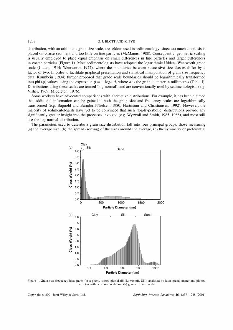
distribution, with an arithmetic grain size scale, are seldom used in sedimentology, since too much emphasis isplaced on coarse sediment and too little on fine particles (McManus, 1988). Consequently, geometric scalingis usually employed to place equal emphasis on small differences in fine particles and larger differencesin coarse particles (Figure 1). Most sedimentologists have adopted the logarithmic Udden–Wentworth gradescale (Udden, 1914; Wentworth, 1922), where the boundaries between successive size classes differ by afactor of two. In order to facilitate graphical presentation and statistical manipulation of grain size frequencydata, Krumbein (1934) further proposed that grade scale boundaries should be logarithmically transformedinto phi (!) values, using the expression ! D ! log2 d, where d is the grain diameter in millimetres (Table I).Distributions using these scales are termed ‘log-normal’, and are conventionally used by sedimentologists (e.g.Visher, 1969; Middleton, 1976).

Some workers have advocated comparisons with alternative distributions. For example, it has been claimedthat additional information can be gained if both the grain size and frequency scales are logarithmicallytransformed (e.g. Bagnold and Barndorff-Nielsen, 1980; Hartmann and Christiansen, 1992). However, themajority of sedimentologists have yet to be convinced that such ‘log-hyperbolic’ distributions provide anysignificantly greater insight into the processes involved (e.g. Wyrwoll and Smith, 1985, 1988), and most stilluse the log-normal distribution.

The parameters used to describe a grain size distribution fall into four principal groups: those measuring(a) the average size, (b) the spread (sorting) of the sizes around the average, (c) the symmetry or preferential

1.5

1.0

0.5

0.0

2.0

2.5

3.0

3.5

4.0

1000 1500 20005000

Cla

ss W

eigh

t (%

)

SandSiltClay

(a)

1.5

1.0

0.5

0.0

2.0

2.5

3.0

3.5

4.0

0.1 1.0 10 100 1000

Cla

ss W

eigh

t (%

)

Clay Silt Sand(b)

Particle Diameter (µm)

Particle Diameter (µm)

Figure 1. Grain size frequency histograms for a poorly sorted glacial till (Lowestoft, UK), analysed by laser granulometer and plottedwith (a) arithmetic size scale and (b) geometric size scale

Copyright ! 2001 John Wiley & Sons, Ltd. Earth Surf. Process. Landforms 26, 1237–1248 (2001)

GRAIN SIZE STATISTICS PROGRAM 1239

Table I. Size scale adopted in the GRADISTAT program, compared with those previously used byUdden (1914), Wentworth (1922) and Friedman and Sanders (1978)

Grain size Descriptive terminology

phi mm/µm Udden (1914) and Friedman and GRADISTAT programWentworth (1922) Sanders (1978)

Very large boulders!11 2048 mm

Large boulders Very large!10 1024

Medium boulders Large!9 512 Cobbles

Small boulders Medium

Boulders!8 256

Large cobbles Small!7 128

Small cobbles Very small!6 64

Very coarse pebbles Very coarse!5 32

Coarse pebbles Coarse!4 16 Pebbles

Medium pebbles Medium

Gravel!3 8

Fine pebbles Fine!2 4

Granules Very fine pebbles Very fine!1 2

Very coarse sand Very coarse sand Very coarse0 1

Coarse sand Coarse sand Coarse1 500 µm

Medium sand Medium sand Medium

Sand2 250

Fine sand Fine sand Fine3 125

Very fine sand Very fine sand Very fine4 63

Very coarse silt Very coarse5 31

Coarse silt Coarse6 16 Silt

Medium silt Medium

Silt7 8

Fine silt Fine8 4

Very fine silt Very fine9 2 Clay

Clay Clay

spread (skewness) to one side of the average, and (d) the degree of concentration of the grains relative tothe average (kurtosis). These parameters can be easily obtained by mathematical or graphical methods. Themathematical ‘method of moments’ (Krumbein and Pettijohn, 1938; Friedman and Johnson, 1982) is the mostaccurate since it employs the entire sample population. However, as a consequence, the statistics are greatlyaffected by outliers in the tails of the distribution, and this form of analysis should not be used unless thesize distribution is fully known (McManus, 1988).



Prior to the availability of modern computers, the calculation of grain size parameters by the method ofmoments was a laborious process. Approximations of the parameters can, however, be obtained by plottingfrequency data as a cumulative frequency curve, extracting prescribed values from the curve and enteringthese into established formulae. Many formulae have been proposed (e.g. Trask, 1932; Krumbein, 1938; Otto,1939; Inman, 1952; McCammon, 1962) although the most widely used are those proposed by Folk and Ward(1957). Such techniques are most appropriate for the analysis of open-ended distributions, since the tails ofthe distribution, which may include extreme outliers, are ignored. With the development of computerized dataanalysis, however, calculation of both method of moments and graphical parameters can be automated, andsome of the original advantages of graphical techniques no longer apply.

THE GRADISTAT PROGRAM

It is with the wide-ranging needs of researchers in geomorphology and sedimentology in mind that theGRADISTAT program has been written. It provides rapid (approximately 50 samples per hour) calculationof grain size statistics by both Folk and Ward (1957) and moments methods. While programs capable ofanalysing grain size data have been published in the past (e.g. Isphording, 1970; Slatt and Press, 1976;McLane, cited in Pye, 1989; Utke, 1997), these are often cumbersome to use or allow little modification forindividual requirements.

The program, written in Microsoft Visual Basic, is integrated into a Microsoft Excel spreadsheet, allowingboth tabular and graphical output. The user is required to input the percentage of sediment present in a numberof size fractions. This can be the weight retained on a series of sieves, or the percentage of sediment detectedin size classes derived from a laser granulometer, X-ray sedigraph or Coulter counter. The following samplestatistics are then calculated: mean, mode(s), sorting (standard deviation), skewness, kurtosis, and a range of

Table II. Statistical formulae used in the calculation of grain size parameters and suggested descriptive terminology,modified from Krumbein and Pettijohn (1938) and Folk and Ward (1957) (f is the frequency in per cent; m is themid-point of each class interval in metric (mm) or phi (m!) units; Px and !x are grain diameters, in metric or phi units

respectively, at the cumulative percentile value of x)

(a) Arithmetic method of moments

Mean Standard deviation Skewness Kurtosis

Nxa D "fmm

100#a D

√

"f$mm ! Nxa%2

100Ska D "f$mm ! Nxa%3

100#a3 Ka D "f$mm ! Nxa%4

100#a4

(b) Geometric method of moments


Nxg D exp"f ln mm

100#g D exp

√

"f$ln mm ! ln Nxg%2

100Skg D "f$ln mm ! ln Nxg%3

100 ln #g3 Kg D "f$ln mm ! ln Nxg%4

100 ln #g4

Sorting (#g) Skewness (Skg) Kurtosis (Kg)

Very well sorted <1"27 Very fine skewed <!1"30 Very platykurtic <1"70Well sorted 1"27–1"41 Fine skewed !1"30 to !0"43 Platykurtic 1"70–2"55Moderately well sorted 1"41–1"62 Symmetrical !0"43 to C0"43 Mesokurtic 2"55–3"70Moderately sorted 1"62–2"00 Coarse skewed C0"43 to C1"30 Leptokurtic 3"70–7"40Poorly sorted 2"00–4"00 Very coarse skewed >C1"30 Very leptokurtic >7"40Very poorly sorted 4"00–16"00Extremely poorly sorted >16"00



(c) Logarithmic method of moments


Nx! D "fm!

100#! D

√

"f$m! ! Nx!%2

100Sk! D "f$m! ! Nx!%3

100#!3 K! D "f$m! ! Nx!%4

100#4!

Sorting (#!) Skewness (Sk!) Kurtosis (K!)

Very well sorted <0"35 Very fine skewed >C1"30 Very platykurtic <1"70Well sorted 0"35–0"50 Fine skewed C0"43 to C1"30 Platykurtic 1"70–2"55Moderately well sorted 0"50–0"70 Symmetrical !0"43 to C0"43 Mesokurtic 2"55–3"70Moderately sorted 0"70–1"00 Coarse skewed !0"43 to !1"30 Leptokurtic 3"70–7"40Poorly sorted 1"00–2"00 Very coarse skewed <!1"30 Very leptokurtic >7"40Very poorly sorted 2"00–4"00Extremely poorly sorted >4"00

(d) Logarithmic (original) Folk and Ward (1957) graphical measures


MZ D !16 C !50 C !84

3#I D !84 ! !16

4C !95 ! !5

6"6SkI D !16 C !84 ! 2!50

2$!84 ! !16%KG D !95 ! !5

2"44$!75 ! !25%

C !5 C !95 ! 2!50

2$!95 ! !5%

Sorting (#1) Skewness (Sk1) Kurtosis (KG)

Very well sorted <0"35 Very fine skewed C0"3 to C1"0 Very platykurtic <0"67Well sorted 0"35–0"50 Fine skewed C0"1 to C0"3 Platykurtic 0"67–0"90Moderately well sorted 0"50–0"70 Symmetrical C0"1 to !0"1 Mesokurtic 0"90–1"11Moderately sorted 0"70–1"00 Coarse skewed !0"1 to !0"3 Leptokurtic 1"11–1"50Poorly sorted 1"00–2"00 Very coarse skewed !0"3 to !1"0 Very leptokurtic 1"50–3"00Very poorly sorted 2"00–4"00 Extremely leptokurtic >3"00Extremely poorly sorted >4"00

(e) Geometric (modified) Folk and Ward (1957) graphical measures

Mean Standard deviation

MG D expln P16 C ln P50 C ln P84

3#G D exp

(

ln P16 ! ln P84

4C ln P5 ! ln P95

6"6

)

Skewness Kurtosis

SkG D ln P16 C ln P84 ! 2$ln P50%2$ln P84 ! ln P16%

C ln P5 C ln P95 ! 2$ln P50%2$ln P25 ! ln P5%

KG D ln P5 ! ln P95

2"44$ln P25 ! ln P75%

Sorting (#G) Skewness (SkG) Kurtosis (KG)

Very well sorted <1"27 Very fine skewed !0"3 to !1"0 Very platykurtic <0"67Well sorted 1"27–1"41 Fine skewed !0"1 to !0"3 Platykurtic 0"67–0"90Moderately well sorted 1"41–1"62 Symmetrical !0"1 to C0"1 Mesokurtic 0"90–1"11Moderately sorted 1"62–2"00 Coarse skewed C0"1 to C0"3 Leptokurtic 1"11–1"50Poorly sorted 2"00–4"00 Very coarse skewed C0"3 to C1"0 Very leptokurtic 1"50–3"00Very poorly sorted 4"00–16"00 Extremely leptokurtic >3"00Extremely poorly sorted >16"00



cumulative percentile values (the grain size at which a specified percentage of the grains are coarser), namelyD10, D50, D90, D90/D10, D90 –D10, D75/D25 and D75 –D25.

In the program, the method of moments is used to calculate statistics arithmetically (based on a normaldistribution with metric size values, seldom used in sedimentology but available with some Coulter sizinginstruments), geometrically (based on a log-normal distribution with metric size values) and logarithmically(based on a log-normal distribution with phi size values), following the terminology and formulae suggestedby Krumbein and Pettijohn (1938). Specified values are then extracted from the cumulative percentage curveusing a linear interpolation between adjacent known points on the curve. These are used to calculate Folk andWard parameters logarithmically (as originally suggested in Folk and Ward (1957), based on a log-normaldistribution with phi size values) and geometrically (based on a log-normal distribution with metric sizevalues). Formulae used in these calculations are presented in Table II.

The statistical parameters are also related to descriptive terms. The mean grain size is described using amodified Udden–Wentworth grade scale (Table I). For terminology to be consistent with the silt and sandfractions, gravel is redefined here as a fraction containing five subclasses ranging from very fine (2 mm) tovery coarse (64 mm). Clasts larger than 64 mm are described as boulders. The terms granule, pebble andcobble have been removed, and it is recommended that their use be reserved for the description of roundedor subrounded clasts. ‘Shingle’ may also be defined simply as rounded gravel. Sorting, skewness and kurtosisare described here using the scheme proposed by Folk and Ward (1957). However, to avoid confusion as towhether skewness terms relate to metric or phi scales, positive skewness is renamed ‘fine skewed’ (indicatingan excess of fines), and negative skewness is renamed ‘coarse skewed’ (indicating a tail of coarser particles).

The program provides a physical description of the textural class (such as ‘muddy sandy gravel’) afterFolk (1954). Also included is a table giving the percentage of grains falling into each size fraction. Forsieving results, the program warns the user if a significant amount (>2 per cent) of sediment has been lostduring analysis. In terms of graphical output, the program provides graphs of the grain size distribution andcumulative distribution of the data in both micrometre and phi units, and displays the sample grain sizeon gravel–sand–mud and sand–silt–clay triangular diagrams. Samples can be analysed individually, or upto 250 samples may be analysed together with all statistics being tabulated. An example printout from theprogram is shown in Figure 2.

TECHNICAL POINTS

To calculate reliably the grain size statistics of a sample, the entire size distribution must be defined. At thecoarse end, there is a requirement to enter at least one size class larger than the largest particles in the sample.At the fine end there is a complication with sediment remaining in the pan after sieving analysis. The largerthe quantity of sediment remaining in the pan, the less accurate the calculation of grain size statistics, withstatistics calculated by the method of moments being most susceptible. Errors in Folk and Ward parametersbecome significant only when the size distribution of more than 5 per cent of the sample is undetermined. If asample contains up to 1 per cent of sediment in the pan the user can either calculate the statistics ignoring thepan fraction, or specify a size which is considered to be representative of the finest particles in the pan, suchas 1 µm (10 !). For samples containing between 1 and 5 per cent of sediment in the pan, it is recommendedthat the pan fraction be ignored and size statistics reported for the sand and gravel fractions only. Samplescontaining more than 5 per cent of sediment in the pan should ideally be further analysed using a differenttechnique, such as sedimentation or laser granulometry, although as noted previously, there are difficulties inmerging data obtained by different methods.

METHOD COMPARISON

Previous studies have compared the statistics derived by moments and graphical methods (e.g. Folk, 1966;Koldijk, 1968; Davis and Ehrlich, 1970; Jaquet and Vernet, 1976; Swan et al., 1978). The ability of GRADI-STAT to analyse rapidly large numbers of samples has allowed the direct comparison of grain size statisticsfor over 800 samples, comprising marine gravels, sands and muds, desert and coastal dune sands, soils and



SAMPLE IDENTITY: Mablethorpe L2D1 ANALYST & DATE: S. Blott, 19/10/2000

SAMPLE TYPE: Unimodal, Well Sorted TEXTURAL GROUP: SandSEDIMENT NAME: Well Sorted Fine Sand

GRAIN SIZE DISTRIBUTION

MODE 1: GRAVEL: COARSE SAND: 0.0%MODE 2: SAND: MEDIUM SAND: 11.0%MODE 3: MUD: FINE SAND: 79.7%

D10: V FINE SAND: 7.7%MEDIAN or D50: V COARSE GRAVEL: V COARSE SILT: 0.5%

D90: COARSE GRAVEL: COARSE SILT: 0.2%(D90 / D10): MEDIUM GRAVEL: MEDIUM SILT: 0.1%(D90 - D10): FINE GRAVEL: FINE SILT: 0.2%(D75 / D25): V FINE GRAVEL: V FINE SILT: 0.3%(D75 - D25): V COARSE SAND: CLAY: 0.2%

Logarithmic"

MEAN : 2.518SORTING (#): 0.670

SKEWNESS (Sk): 5.522KURTOSIS (K ): 48.69

0.523

51.64

SAMPLE STATISTICS

126.1

METHOD OF MOMENTS

"2.432

2.4550.390

$0.1793.852

µm

µm µm µm

185.5

126.8184.1252.91.994

1.9842.4412.9791.5020.996

Geometric

174.8

Arithmetic

186.2

1.43766.79

1.239

1.591$5.52248.69

182.51.311

$0.0911.025

Geometric Logarithmic

SymmetricalMesokurtic

Description

Fine SandWell Sorted

"

0.0901.024

FOLK & WARD METHOD

0.0%98.4%1.6%

0.0%0.0%0.0%0.0%0.0%0.0%

GRAIN SIZE DISTRIBUTION

0.0

2.0

4.0

6.0

8.0

10.0

12.0

14.0

0.01.02.03.04.05.06.07.08.09.010.0Particle Diameter (")

1 10 100 1000Particle Diameter (µm)

)(x

Cla

ss W

eigh

t (%

)

Figure 2. Example GRADISTAT printout, with logarithmic frequency plot, for a coastal dune sand (Lincolnshire, UK)

glacial tills. The relationships between graphical and moment parameters are illustrated in Figures 3 and 4for geometric and logarithmic statistics. While arithmetic statistics have been included in the GRADISTATprogram for reasons of completeness, it is recommended that the more representative geometric or logarithmicstatistics be used to characterize sediments as general practice.

It is clear that relationships between the methods are similar for geometric and logarithmic statistics.Geometric mean and sorting values for either method are related to their logarithmic counterparts by simplelogarithmic relationships. Geometric and logarithmic skewness parameters are inversely related since metricand phi scales operate in opposite directions, while geometric and logarithmic kurtosis values are identical.



1

10

100

1000

10000

1 10 100 1000 10000Geometric Mean by Moments Method (µm) (log scale)

Geom

etric Mean by G

raphicalM

ethod (µm) (log scale)

Gravel

Sand

Silt

Clay

1.0

10.0

1.0 10.08.06.04.02.0

8.06.0

4.0

2.0

Very well sortedWell sorted

Moderately well sortedModerately sorted

Poorly sorted

Very poorly sorted

Geometric Sorting by Moments Method (log scale)

Geom

etric Sorting by

Graphical M

ethod (log scale)

$0.8

$0.4

0.0

0.4

0.8

$6.0 $4.0 $2.0 0.0 2.0 4.0 6.0Geometric Skewness by Moments Method

Geom

etric Skew

ness byG

raphical Method

SymmetricalCoarse skewed

Fine skewed

Very fine skewed

Very coarse skewed

0.4

0.60.81.0

2.0

4.0

6.0

60.040.020.010.08.06.04.02.01.0

Very platykurtic

PlatykurticMesokurticLeptokurtic

Very leptokurtic

Geometric Kurtosis by Moments Method (log scale)

Geom

etric Kurtosis by

Graphical M

ethod (log scale)

Figure 3. Comparison of statistical parameters calculated using the geometric method of moments and Folk and Ward (1957) graphicalmethod. Analysed samples are marine gravels, sands and muds, desert and coastal dune sands, soils and glacial tills

The relationships between graphical and moment parameters can be explained by differences in the emphasiseach method places on different parts of the grain size distribution. The graphical method places more weighton the central portion of the grain size curve and less on the tails. The upper and lower limits of calculations



0.4

0.60.81.0

2.0

4.0

6.0

60.040.020.010.08.06.04.02.01.0

Very platykurtic

PlatykurticMesokurticLeptokurtic

Very leptokurtic

Logarithmic Kurtosis by Moments Method (log scale)

Logarithmic K

urtosis byG

raphical Method (log scale)

$0.8

$0.4

0.0

0.4

0.8

$6.0 $4.0 $2.0 0.0 2.0 4.0 6.0

Logarithmic S

kewness by

Graphical M

ethod

Logarithmic Skewness by Moments Method

SymmetricalFine skewed

Coarse skewed

Very coarse skewed

Very fine skewed

0.0

0.5

1.0

1.5

2.0

2.5

3.0

0.0 0.5 1.0 1.5 2.0 2.5 3.0

Logarithmic S

orting byG

raphical Method

Logarithmic Sorting by Moments Method

Very well sortedWell sorted

Moderately well sortedModerately sorted

Poorly sorted

Very poorly sorted

$4.0

$2.0

0.0

2.0

4.0

6.0

8.0

10.0

$4.0 $2.0 0.0 2.0 4.0 6.0 8.0 10.0

Logarithmic M

ean byG

raphical Method (phi)

Logarithmic Mean by Moments Method (phi)

Gravel

Sand

Silt

Clay

$

Figure 4. Comparison of statistical parameters calculated using the logarithmic method of moments and Folk and Ward (1957) graphicalmethod. Analysed samples are marine gravels, sands and muds, desert and coastal dune sands, soils and glacial tills

are at 95 and 5 per cent of the distribution respectively, and sediment outside these limits is ignored. The firstorder moment measure (mean) also places more emphasis on the central portion of the curve, and consequentlythe graphical mean closely approximates the moment mean (Figures 3 and 4).



With higher order moments, however, parameters become more sensitive to the tails of the distribution.While there is clearly a linear relationship between graphical and moment sorting, there is better agreementfor well sorted sediments (low sorting values), since grains are concentrated in the central portion of thegrain size distribution. For less well sorted sediments, the graphical method generally produces better sortingvalues since sediment in the tails of the distribution is ignored. The difference is greatest for samples thatare well sorted except for a fine or coarse tail representing less than 5 per cent of the sample weight (such asthe dune sand shown in Figure 2). Alternatively, graphical sorting can exceed moment sorting if the centralportion of the distribution is the least sorted, such as for multimodal sediments (Swan et al., 1978).

With the highest order moments of skewness and kurtosis, the differences between the methods becomemuch greater. While skewness values are comparable for log-normally distributed sediments (skewness valueof zero), kurtosis parameters are inherently different, since a log-normal distribution takes a value of 1"0for the graphical method and 3"0 for the method of moments. The convention used by some authors (e.g.Krumbein and Pettijohn, 1938) to subtract 3"0 from the moments value to standardize the measure aroundzero is not followed here. Values higher than 1"0 (or 3"0) indicate a leptokurtic (strongly peaked) distribution,smaller values a platykurtic (relatively flat) distribution. For sediments that are far from log-normal, the higherorder moments of sorting, skewness and kurtosis interact in complicated ways (Swan et al., 1978). The resultis that as skewness and kurtosis increase, the percentage of sediment in the tails of the distribution increases,and the relationships between the graphical and moment parameters break down.

One of the advantages of the Folk and Ward method is the opportunity to convert parameter values todescriptive terms for the sediment. The relationships illustrated in Figures 3 and 4, although unclear in someinstances, have been used to assign corresponding descriptive terms to geometric and logarithmic momentvalues, presented in Table II. These terms are intended as a guide only, since it is clear from the previousdiscussion that higher order parameters can be difficult to interpret. Sorting in particular is known to be asinusoidal function of mean grain size, with medium and fine sands generally exhibiting better sorting thanclays, silts and gravels (Inman, 1949; Folk and Ward, 1957).

OTHER DESCRIPTORS

A variety of alternative parameters can be used to differentiate between different sediments. Engineers com-monly quote the median, or D50 size value, together with a measure of dispersion, such as D90/D10, D90 –D10or D75 –D25 (the interquartile range). For soils work, where the materials in question are commonly multi-modal, it may be most appropriate simply to cite the values for the primary, secondary and tertiary modes,the median, and a measure of distribution spread, such as D90 –D10. These descriptors are provided by theGRADISTAT software and frequently prove to be more reliable than the standard size statistics, especiallywhen sediments are clearly multimodal.

DISCUSSION AND CONCLUSIONS

Although the GRADISTAT program is extremely flexible in terms of input and output, it remains the respon-sibility of the user to interpret the results in a manner appropriate to the questions being addressed. Careshould be taken when interpreting open-ended distributions, or where the sediment is not unimodal. It shouldalso be noted that all methods of particle size analysis are influenced by factors such as grain shape, density,and sometimes optical properties. While some methods specify grain size frequency per unit weight, othersspecify grain size per unit volume. It is therefore not appropriate to compare directly results obtained usingdifferent methods. In some instances, however, it may be possible to apply calibration factors.

Comparison of the Folk and Ward graphical method and the method of moments has indicated that bothmethods have drawbacks. The graphical method is relatively insensitive to sediments containing a largeparticle size range in the tails of the distribution. This can be either an advantage or a disadvantage dependingon the particular problem under study. The moment method can equally overemphasize the importance oflong tails with low frequencies, and in these circumstances the Folk and Ward method is likely to describemore accurately the general characteristics of the bulk of the sample. Previous workers have been divided



about the relative merits of graphical and moment statistics. If only the mean grain size and sorting values arerequired, the graphical and moments methods produce similar results. If, however, the skewness or kurtosisare to be determined, in our experience the Folk and Ward measures provide the most robust basis forroutine comparisons of compositionally variable sediments. Although most sedimentologists have traditionallyworked with phi units, in our opinion statistics expressed geometrically (in metric units) are to be preferredto logarithmic statistics (in phi units), since the phi scale is seldom used amongst biologists, archaeologists,soil scientists or engineers, and results are easier to visualize. Any study incorporating grain size analysismust include a clear statement of the measurement technique and the method used in the calculation of anystatistics. In many circumstances it will be appropriate to employ more than one method, since comparisonof results obtained in different ways may provide additional insight into the processes involved.

ACCESSING THE SOFTWARE

The universal availability of Microsoft Excel should enable use of the GRADISTAT program by many workers,and allow efficient transfer of data and statistics between other applications. The file GRADISTAT.xls is com-patible with Microsoft Excel 97 or 2000 (versions 8.0 and 9.0), and can be downloaded from the Earth SurfaceProcesses and Landforms software web site (URL: http://www.interscience.wiley.com/jpages/0197–9337/sites.html).

ACKNOWLEDGEMENTS

This work was undertaken while S. J. Blott was in receipt of NERC Studentship GT04/97/250/MS. Additionalfunding was provided by a CASE Award with the Environment Agency. The authors would like to thankJ. Jack and D. Thornley at the Postgraduate Research Institute for Sedimentology at the University of Reading,UK, for their encouragement in the creation of the program, and J. Richards and S. Saye who assisted intesting the program.

REFERENCES

Bagnold RA, Barndorff-Nielsen OE. 1980. The pattern of natural grain size distributions. Sedimentology 27: 199–207.Bui EN, Mazullo J, Wilding LP. 1990. Using quartz grain size and shape analysis to distinguish between aeolian and fluvial deposits

in the Dallol Bosso of Niger (West Africa). Earth Surface Processes and Landforms 14: 157–166.Davis MW, Ehrlich R. 1970. Relationships between measures of sediment-size-frequency distributions and the nature of sediments.

Geological Society of America Bulletin 81: 3537–3548.Folk RL. 1954. The distinction between grain size and mineral composition in sedimentary-rock nomenclature. Journal of Geology 62:

344–359.Folk RL. 1966. A review of grain-size parameters. Sedimentology 6: 73–93.Folk RL, Ward WC. 1957. Brazos River bar: a study in the significance of grain size parameters. Journal of Sedimentary Petrology 27:

3–26.Friedman GM. 1979. Differences in size distributions of populations of particles among sands of various origins. Sedimentology 26:

3–32.Friedman GM, Johnson KG. 1982. Exercises in Sedimentology . Wiley: New York.Friedman GM, Sanders JE. 1978. Principles of Sedimentology . Wiley: New York.Hartmann D, Christiansen C. 1992. The hyperbolic shape triangle as a tool for discriminating populations of sediment samples of closely

connected origin. Sedimentology 39: 697–708.Inman DL. 1949. Sorting of sediments in the light of fluid mechanics. Journal of Sedimentary Petrology 19: 51–70.Inman DL. 1952. Measures for describing the size distribution of sediments. Journal of Sedimentary Petrology 22: 125–145.Isphording WC. 1970. FORTRAN IV program for calculation of measures of central tendency and dispersion on IBM 360 computer.

Journal of Geology 78: 626–628.Jaquet JM, Vernet JP. 1976. Moment and graphic size parameters in sediments of Lake Geneva (Switzerland). Journal of Sedimentary

Petrology 46: 305–312.Koldijk WS. 1968. On environment-sensitive grain-size parameters. Sedimentology 10: 57–69.Krumbein WC. 1934. Size frequency distributions of sediments. Journal of Sedimentary Petrology 4: 65–77.Krumbein WC. 1938. Size frequency distribution of sediments and the normal phi curve. Journal of Sedimentary Petrology 8: 84–90.Krumbein WC, Pettijohn FJ. 1938. Manual of Sedimentary Petrography . Appleton-Century-Crofts: New York.McCammon RB. 1962. Efficiencies of percentile measures for describing the mean size and sorting of sedimentary particles. Journal

of Geology 70: 453–465.McManus J. 1988. Grain size determination and interpretation. In Techniques in Sedimentology , Tucker M (ed.). Blackwell: Oxford;

63–85.



Middleton GV. 1976. Hydraulic interpretation of sand size distributions. Journal of Geology 84: 405–426.Otto GH. 1939. A modified logarithmic probability graph for the interpretation of mechanical analyses of sediments. Journal of Sedi-

mentary Petrology 9: 62–75.Pye K. 1989. GRANNY: a package for processing grain size and shape data. Terra Nova 1: 588–590.Pye K. 1994. Properties of sediment particles. In Sediment Transport and Depositional Processes , Pye K (ed.). Blackwell: Oxford;

1–24.Slatt RM, Press DE. 1976. Computer program for presentation of grain-size data by the graphic method. Sedimentology 23: 121–131.Swan D, Clague JJ, Luternauer JL. 1978. Grain size statistics I: evaluation of the Folk and Ward graphic measures. Journal of Sedi-

mentary Petrology 48: 863–878.Trask PD. 1932. Origin and Environment of Source Sediments of Petroleum . Gulf Publishing Company: Houston.Udden JA. 1914. Mechanical composition of clastic sediments. Bulletin of the Geological Society of America 25: 655–744.Utke A. 1997. SediVision 2.0 . Springer-Verlag: Heidelberg.Visher GS. 1969. Grain size distributions and depositional processes. Journal of Sedimentary Petrology 39: 1074–1106.Wentworth CK. 1922. A scale of grade and class terms for clastic sediments. Journal of Geology 30: 377–392.Wyrwoll KH, Smith GK. 1985. On using the log-hyperbolic distribution to describe the textural characteristics of eolian sediments.

Journal of Sedimentary Petrology 55: 471–478.Wyrwoll KH, Smith GK. 1988. On using the log-hyperbolic distribution to describe the textural characteristics of eolian sediments:

reply. Journal of Sedimentary Petrology 58: 161–162.


gradistat

Documents