Graduate Macro Theory II:

The Real Business Cycle Model

Eric Sims

University of Notre Dame

Spring 2011

1 Introduction

This note describes the canonical real business cycle model. A couple of classic references here are

Kydland and Prescott (1982), King, Plosser, and Rebelo (1988), and King and Rebelo (2000).

2 The Decentralized Model

I will set the problem up as a decentralized model, studying first the behavior of households and

then the behavior of firms.

There are two primary ways of setting the model up, which both yield identical solutions. In

both households own the firms, but management and ownership are distinct, and so households

behave as though firm profits are given. In one formulation firms own the capital stock, and issue

both debt and equity to households. In another formulation, households own the capital stock

and rent it to firms; firms still issue debt and equity to households. We will go through both

formulations. Intuitively these set-ups have to be the same because, either way, households own

the capital stock (either directly or indirectly).

In both setups I abstract from trend growth, which, as we have seen, does not really make much

of a difference anyway.

2.1 Firms Own the Capital Stock

Here we assume that firms own the capital stock. We begin with the household problem.

2.1.1 Household Problem

Households discount the future by β < 1. They supply labor (measured in hours), nt and consume,

ct. They get utility from consumption and leisure; with the time endowment normalized to unity,

leisure is 1 − nt. They earn a wage rate, wt, which they take as given. They hold bonds, bt,

which pay interest rate rt. bt > 0 means that the household has a positive stock of savings; bt < 0

1

means the household has a stock of debt. Note that “savings” is a stock; “saving” is a flow. The

households take the interest rate as given. Their budget constraint says that each period, total

expenditure must equal total income. Household earn wage income, wtnt, have profit distributions

in the form of dividends, Πt, and interest income on existing bond holds, rtbt (note this can be

negative, so that there is an interest cost of servicing debt). Household expenditure is composed of

consumption, ct and saving, bt+1 − bt (i.e. the accumulation of new savings). Hence we can write

the constraint:

ct + (bt+1 − bt) = wtnt + Πt + rtbt (1)

Note a timing convention – rt is the interest you have to pay today on existing debt. rt+1 is

what you will have to pay tomorrow, but you choose how much debt to take into tomorrow today.

Hence, we assume that households observe rt+1 in time t. Hence we can treat rt+1 as known from

the perspective of time t. Households choose consumption, work effort, and the new stock of savings

each period to maximize the present discounted value of welfare:

maxct,nt,bt+1

Et

∞∑t=0

βt (u(ct) + v(1− nt))

s.t.

ct + bt+1 = wtnt + Πt + (1 + rt)bt

We can form a current value Lagrangian:

L = E0

∞∑t=0

βt (u(ct) + v(1− nt) + λt(wtnt + Πt + (1 + rt)bt − ct − bt+1))

The first order conditions characterizing an interior solution are:

∂L∂ct

= 0⇔ u′(ct) = λt (2)

∂L∂nt

= 0⇔ v′(1− nt) = λtwt (3)

∂L∂bt+1

= 0⇔ λt = βEtλt+1(1 + rt+1) (4)

These can be combined together to yield:

2

u′(ct) = βEt(u′(ct+1)(1 + rt+1)

)(5)

v′(1− nt) = u′(ct)wt (6)

(5) and (6) have very intuitive, intermediate micro type interpretations. (5) says to equate

the marginal rate of substitution between consumption today and tomorrow (i.e. u′(ct)βu′(ct+1)

) to

the relative price of consumption today (i.e. 1 + rt+1). (6) says to equate the marginal rate of

substitution between leisure and consumption (i.e. v′(1−nt)u′(ct)

) to the relative price of leisure (i.e. wt).

In addition, there is the transversality condition:

limt→∞

βtbt+1u′(ct) = 0 (7)

2.1.2 The Firm Problem

The firm wants to maximize the present discounted value of (real) net revenues (i.e. cash flows). It

discounts future cash flows by the stochastic discount factor. The stochastic discount factor puts

cash flows (measured in goods) in terms of current utils (if we take the current period to be t = 0,

this means . Define the stochastic discount factor as:

Mt = βtE0u′(ct)

The firm discounts by this because this is how consumers value future dividend flows. One unit

of dividends returned to the household at time t generates u′(ct) additional units of utility, which

must be discounted back to the present period (which we take to be 0), by βt. The firm produces

output, yt, according to a constant returns to scale production function, yt = atf(kt, nt), with the

usual properties. It hires labor, purchases new capital goods, and issues debt. I denote its debt as

dt, and it pays interest on its debt, rt. Its revenue each period is equal to output. Its costs each

period are the wage bill, investment in new physical capital, and services costs on its debt. It can

raise its cash flow by issuing new debt (i.e. dt+1 − dt raises cash flow). It discounts future cash

flows by the expected real interest rate. Its problem can be written as:

maxnt,It,dt+1

V0 = E0

∞∑t=0

Mt (atf(kt, nt)− wtnt − It + dt+1 − (1 + rt)dt)

s.t.

kt+1 = It + (1− δ)kt

3

We can re-write the problem by imposing that the constraint hold each period:

maxnt,It,dt+1

V0 = E0

∞∑t=0

Mt (atf(kt, nt)− wtnt − kt+1 + (1− δ)kt + dt+1 − (1 + rt)dt)

The first order conditions are as follows:

∂V0∂nt

= 0⇔ atfn(kt, nt) = wt (8)

∂V0∂kt+1

= 0⇔ u′(c)t = βEt(u′(ct+1)((at+1fk(kt+1, nt+1) + (1− δ)) (9)

∂V0∂dt+1

= 0⇔ u′(ct) = βEt(u′(ct+1)(1 + rt+1)) (10)

(9) and (10) follow from the fact that Mt = βtu′(ct) and EtMt+1 = βt+1u′(ct+1). Note that (10)

is the same as (5), and therefore must hold in equilibrium as long as the household is optimizing.

This means that the amount of debt the firm issues is indeterminate, since the condition will hold

for any choice of dt+1. This is essentially the Modigliani-Miller theorem – it doesn’t matter how

the firm finances its purchases of new capital – debt or equity – and hence the debt/equity mix is

indeterminate.

2.1.3 Closing the Model

To close the model we need to specify a stochastic process for the exogenous variable(s). The only

exogenous variable in the model is at. We assume that it is well-characterized as following a mean

zero AR(1) in the log (we have abstracted from trend growth):

ln at + ρ ln at−1 + εt (11)

2.1.4 Equilibrium

A competitive equilibrium is a set of prices (rt+1, wt) and allocations (ct, nt, kt+1, dt+1, bt+1) taking

kt, dt, bt, at and the stochastic process for at as given; the optimality conditions (5) - (7), (8)-

(10), and the transversality condition holding; the labor and bonds market clearing (ndt = nst and

bt+1 = dt+1); and both budget constraints holding with equality.

Let’s consolidate the household and firm budget constraints:

ct + (bt+1 − bt) = wtnt + rtbt + atf(kt, nt)− wtnt − It + dt+1 − (1 + rt)dt (12)

⇒ (13)

atf(kt, nt) = ct + It (14)

4

In other words, bond market-clearing plus both budget constraints holding just gives the stan-

dard accounting identity that output must be consumed or invested.

2.2 Households Own the Capital Stock

Now we consider a version of the decentralized problem in which the households own the capital

stock and rent it to firms. Otherwise the structure of the problem is the same.

2.2.1 Household Problem

As before, households consume and supply labor. Now they also own the capital stock. They earn

a rental rate for renting out the capital stock to firms each period, Rt. The household budget

constraint is:

ct + kt+1 − (1− δ)kt + bt+1 − bt = wtnt +Rtkt + rtbt + Πt (15)

The household has income comprised of labor income, capital income, interest income, and

profits (again it takes profits as given). It can consume this, accumulate more capital (this is the

kt+1 − (1− δ)kt term), or accumulate more saving. Its problem is:

maxct,nt,kt+1,bt+1

E0

∞∑t=0

βt (u(ct) + v(1− nt))

s.t.

ct + kt+1 − (1− δ)kt + bt+1 − bt = wtnt +Rtkt + rtbt + Πt

Form a current value Lagrangian:

L = E0

∞∑t=0

βt (u(ct) + v(1− nt) + λt(wtnt +Rtkt + (1 + rt)bt + Πt − ct − kt+1 + (1− δ)kt − bt+1))

The first order conditions are:

∂L∂ct

= 0⇔ u′(ct) = λt (16)

∂L∂nt

= 0⇔ v′(1− nt) = λtwt (17)

∂L∂kt+1

= 0⇔ λt = βEtλt+1(Rt+1 + (1− δ)) (18)

∂L∂bt+1

= 0⇔ λt = βEtλt+1(1 + rt+1) (19)

5

These first order conditions can be combined to yield:

v′(1− nt) = u′(ct)wt (20)

u′(ct) = βEtu′(ct+1)(Rt+1 + (1− δ)) (21)

u′(ct) = βEtu′(ct+1)(1 + rt+1) (22)

Note that (20) and (21) are the same as (5) and (9). (22) is the same as (6). One is tempted to

claim that rt+1 + δ = Rt+1 given that (19) and (20) must both hold. This is not quite right. rt+1

is known at time t; Rt+1 is not. Hence one can take 1 + rt+1 outside of the expectations operator

in (23) to get:

1 + rt+1 =u′(ct)

βEtu′(ct+1)

But once cannot do the same for (22). Intuitively, Et(u′(ct+1)(Rt+1+(1−δ) = Et(u

′(ct+1)Et(Rt+1+

(1−δ))+cov(u′(ct+1), Rt+1). In general, that covariance term is not going to be zero. It is likely to

be negative –as we will see, EtRt+1 is the expected marginal product of capital. When the marginal

product of capital is high (so Rt+1 is high), then consumption is likely to be high (because MPK

being high probably means that TFP is high), which means that marginal utility of consumption is

low. To be compensated for holding an asset whose return covaries negatively with consumption,

the household would demand a premium over the safe, riskless return rt+1.

In a linearization of the model, that covariance term would drop out, and we could say that

rt+1 = EtRt+1 − δ, but in general there is another term that is essentially the equity premium.

2.2.2 The Firm Problem

The firm problem is similar to before, but now it doesn’t choose investment. Rather, it chooses

capital today given the rental rate, Rt. Note that the firm can vary capital today even though the

household cannot given that capital is predetermined. The labor choice and debt choice are similar.

Again, the firm wants to maximize the present discounted value of cash flows.

maxnt,kt,dt+1

V0 = (1 + r0)E0

∞∑t=0

Mt (atf(kt, nt)− wtnt −Rtkt + dt+1 − (1 + rt)dt)

The first order conditions are:

6

∂V0∂nt

= 0⇔ atfn(kt, nt) = wt (23)

∂V0∂kt

= 0⇔ atfk(kt, nt) = Rt (24)

∂V0∂dt+1

= 0⇔ u′(ct) = βEtu′(ct+1)(1 + rt+1) (25)

(25) follows from the definition of the stochastic discount factor, and again is automatically

satisfied; so again the amount of debt is indeterminate.

2.2.3 Equivalence to the Other Setup

Plug (24) into (21) and you get:

u′(ct) = βEt(u′(ct+1)(at+1fk(kt+1, nt+1) + (1− δ)) (26)

This is identical to (9). Also, (20) is equivalent to (6); (5) is equivalent to (22); and (23) is the

same as (8). Hence, all the first order conditions are the same. The definition of equilibrium is the

same. Both the firm and household budget constraints holding again give rise to the accounting

identity (14). Hence, these setups give rise to identical solutions. It simply does not matter whether

households own the capital stock and lease it to firms or whether firms own the capital stock. Since

households own firms, these are equivalent ownership structures.

3 Equilibrium Analysis of the Decentralized Model

We can combined first order conditions from the firm and household problems (in either setup) to

yield the equilibrium conditions:

u′(ct) = βEt(u′(ct+1)(at+1fk(kt+1, nt+1) + (1− δ)

)(27)

v′(1− nt) = u′(ct)atfn(kt, nt) (28)

kt+1 = atf(kt, nt)− ct + (1− δ)kt (29)

ln at = ρ ln at−1 + εt (30)

yt = atf(kt, nt) (31)

yt = ct + It (32)

u′(ct) = βEtu′(ct+1)(1 + rt+1) (33)

wt = atfn(kt, nt) (34)

(27) can essentially be interpreted as an investment-saving equilibrium. (28) characterizes

equilibrium in the labor market, since the wage is equal to the marginal product of capital. (29)

7

is just the capital accumulation equation, and (31) is the exogenous process for technology. (31)

defines output and (32) defines investment. (33) and (34) just give us back the equilibrium factor

prices. We have 1 truly forward-looking variable (consumption); two state/exogenous variables

(capital and TFP); and five static variables (hours, output, investment, the real interest rate, and

the real wage). That’s a total of eight variables and we have eight equations.

We need to specify functional forms. For simplicity, assume that u(ct) = ln ct and v(1− nt) =

θ ln(1− nt). Assume that the production function is Cobb-Douglas: yt = atkαt n

1−αt .

Given these parameter values we can analyze the steady state. The steady state is a situation

in which a∗ = 1 (its unconditional mean), kt+1 = kt = k∗, and ct+1 = ct = c∗. Given the steady

state values of these variables, the steady state values of the static variables can be backed out. We

can most easily solve for the steady state by beginning with the dynamic Euler equation, (27).

1 = β(αk∗α−1n∗1−α + (1− δ))

Let’s use this to solve for the steady state capital to labor ratio (life is much easier if you do it

this way):

1

β− (1− δ) = α

(k∗

n∗

)α−1⇒

k∗

n∗=

(α

1β − (1− δ)

) 11−α

(35)

Given the steady state capital-labor ratio, we now have the steady state factor prices:

w∗ = (1− α)

(k∗

n∗

)α(36)

r∗ = α

(k∗

n∗

)α−1− δ (37)

In the steady state, I∗ = k∗. Hence, in terms of the capital-labor ratio:

I∗ = δ

(k∗

n∗

)n∗ (38)

Steady state output is:

y∗ =

(k∗

n∗

)αn∗ (39)

Steady state consumption then comes from the accounting identity:

8

c∗ = n∗((

k∗

n∗

)α− δ

(k∗

n∗

))(40)

Hence, I’ve solved for the steady state of all variables taken n∗ as given. I could do this the

“hard way” and solve for n∗, but I don’t really need to do that. As we saw in the last problem set,

n∗ is a function of θ and other parameters. θ otherwise doesn’t show up in any of the steady state

expressions above. Hence, given other parameters, there will be a one to one mapping between

θ and n∗. It’s easier to just leave it like this, kind of treating n∗ as a parameter (which it is,

effectively, see below).

We next need to specify parameters values. We can undertake a calibration exercise just as

we did in the basic neoclassical model. We can pin down α by looking at average labor’s share

of income. We can pin down β by looking the average real interest rate. We can pin down δ by

looking at the average ratio of investment to output. We can pin down θ by imposing that steady

state hours equal the average fraction of time spent working (typically we impose n∗ = 0.2 to 0.33,

depending on how we defines the time endowment (e.g. 16 hours per day or 24 hours per day,

etc..). It’s in this sense that we can treat n∗ as a parameter (see the above paragraph).

Given the parameter values and steady states, we can solve for the policy function(s). Again,

the system can be reduced to just the forward-looking and state variables, so we can reduce this to

a system of (non-linear) difference equations in three variables (consumption, capital, and TFP).

The policy function is a mapping between capital and TFP into consumption. There are additional

policy functions that can then be backed out for output, investment, and employment. Given all

these policy functions we can then back out the equilibrium prices (real interest rate and real wage

rate). We could find these policy functions either through a dynamic programming approach or

through log-linear approximation. We can then conduct “quantitative analysis” on the model.

Before we do that, let’s try to do some “qualitative analysis” to get an idea of how the model

actually works. To do this, I’m going to log-linearize the first order conditions about the non-

stochastic steady state. Start by taking logs of the static labor supply condition (28):

ln θ − ln(1− nt) = − ln ct + ln(1− α) + ln at + α ln kt − α lnnt

The linearization (here I’m going to ignore the evaluation at steady state, which cancels out)

is:

nt − n∗

1− n∗= −ct − c

∗

c∗+at − a∗

a∗+ α

kt − k∗

k∗− αnt − n

∗

n∗

Simplify into our “tilde” notation:

(n∗

1− n∗

)nt = −ct + at + αkt − αnt

9

So as to economize on notation, let’s denote γ = n∗

1−n∗ > 0. Then we get:

nt = −(

1

γ + α

)ct +

(1

γ + α

)at +

(α

γ + α

)kt (41)

Now let’s linearize the accumulation equation. Begin by taking logs:

ln kt+1 = ln(atkαt n

1−αt − ct + (1− δ)kt)

Now linearize, again ignoring the evaluation at steady state part, which cancels out anyway:

kt+1 − k∗

k∗=

1

k∗(k∗αn∗1−α(at − a∗) + αk∗α−1n∗1−α(kt − k∗) + . . .

+(1− α)k∗αn∗−α(nt − n∗)− (ct − c∗) + (1− δ)(kt − k∗))

Now simplify and use our “tilde” notation to denote the percentage deviation of a variable from

its steady state:

kt+1 =

(k∗

n∗

)α−1 (at + αkt + (1− α)nt

)− c∗

k∗ct + (1− δ)kt

kt+1 =1

βkt +

(k∗

n∗

)α−1at + (1− α)

(k∗

n∗

)α−1nt −

c∗

k∗ct

The last simplification follows from the fact that αk∗α−1n∗1−α + (1 − δ) = 1β . Now substitute

the log-linearized expression for employment into this expression:

kt+1 =

(1

β+

1− αγ + α

α

(k∗

n∗

)α−1)kt +

((k∗

n∗

)α−1( 1 + γ

γ + α

))at −

(c∗

k∗+

1− αγ + α

(k∗

n∗

)α−1)ct

(42)

Now we need to log-linearize the consumption Euler equation. Begin by taking logs:

− ln ct = lnβ − ln ct+1 + ln(αat+1k

α−1t+1 n

1−αt+1 + (1− δ)

)Now linearize, ignoring the evaluation at steady state and making use of the fact that αk∗α−1n∗1−α+

(1− δ) = 1β :

−ct − c∗

c∗= −ct+1 − c∗

c∗+ β

(αk∗α−1n∗1−α(at+1 − a∗) + (α− 1)αk∗α−2n∗1−α(kt+1 − k∗) + . . .

+(1− α)αk∗α−1n∗−α(nt+1 − n∗))

10

This can be simplified using our tilde notation:

−ct = −ct+1 + βα

(k∗

n∗

)α−1 (at+1 + (α− 1)kt+1 + (1− α)nt+1

)(43)

Now eliminate nt+1 using (41):

−ct = −ct+1 + βα

(k∗

n∗

)α−1at+1 + βα(α− 1)

(k∗

n∗

)α−1kt+1 + . . .

· · ·+ βα(1− α)

(k∗

n∗

)α−1(−(

1

γ + α

)ct+1 +

(1

γ + α

)at+1 +

(α

γ + α

)kt+1

)Simplifying:

−ct = −

(1 + βα(1− α)

(k∗

n∗

)α−1( 1

γ + α

))ct+1 +

(βα

(k∗

n∗

)α−1)( 1 + γ

γ + α

)at+1 + . . .

· · · −

(βα(1− α)

(k∗

n∗

)α−1)( γ

γ + α

)kt+1 (44)

Equations (42) and (44) (plus the exogenous process for TFP) define a system of linearized

difference equations. Let’s try to think about this in the context of a phase diagram. The ct+1 = ct

isocline can be solved for from (44):

βα(1− α)

(k∗

n∗

)α−1( 1

γ + α

)ct+1 =

(βα

(k∗

n∗

)α−1)( 1 + γ

γ + α

)at+1 −

(βα(1− α)

(k∗

n∗

)α−1)( γ

γ + α

)kt+1

This simplifies greatly to yield:

ct+1 =

(1 + γ

1− α

)at+1 − γkt+1

To make things easier, evaluate this at t (we gain engage in the abuse of terminology in treating

the two time periods as approximately the same):

ct =

(1 + γ

1− α

)at − γkt (45)

This is the ct+1 = ct = 0 isocline – i.e. the set of (ct, kt) pairs where consumption is constant.

In (ct, kt) space it is downward sloping, and it will shift up if at were to change.

Now go to (42) to find the kt+1 = kt = 0 isocline:

11

(c∗

k∗+

1− αγ + α

(k∗

n∗

)α−1)ct =

(1

β− 1 +

1− αγ + α

α

(k∗

n∗

)α−1)kt +

((k∗

n∗

)α−1( 1 + γ

γ + α

))at

Simplify a bit:

ct =

(c∗

k∗+

1− αγ + α

(k∗

n∗

)α−1)−1(( 1

β− 1 +

1− αγ + α

α

(k∗

n∗

)α−1)kt +

((k∗

n∗

)α−1( 1 + γ

γ + α

))at

)(46)

This is upward-sloping in kt. Furthermore, we actually know that the coefficient on the capital

stock must be less than one. The coefficient can be written as follows:

(c∗

k∗+

1− αγ + α

(k∗

n∗

)α−1)−1(( 1

β− 1 +

1− αγ + α

α

(k∗

n∗

)α−1))

We know that 1−αγ+α > α(1−α)

γ+α since 0 < α < 1. Hence, we can prove that this coefficient is

less than unity if we can show that 1β − 1 is less than c∗

k∗ (because this would be sufficient to show

that the numerator is less than the denominator, and hence the total coefficient is less than unity).

We can find an expression for the consumption-capital ratio in the steady state by looking at the

accounting identity and simplifying:

c∗ = k∗αn∗1−α − δk∗

c∗

k∗=

(k∗

n∗

)α−1− δ

c∗

k∗=

1β − (1− δ)

α− δ

c∗

k∗=

1β − 1

α+ δ

(1− αα

)This has to be great than 1

β − 1, since 0 < α < 1 and δ > 0.

We thus have two isoclines. We want to plot these in a plane with ct on the vertical axis and

kt on the horizontal axis. When at = 0 (i.e. we were at the unconditional mean of technology), it

is clear that the two isoclines cross at the point ct = kt = 0 – i.e. they cross at the non-stochastic

steady state. We have that the ct+1− ct = 0 isocline is downward sloping and that the kt+1− kt = 0

isocline is downward sloping.

We want to examine the dynamics off of the isoclines so as to locate the saddle path. Quite

intuitively, if kt is “too big” relative to what it would be when ct+1 − ct = 0 – i.e. we are to the

right of the ct+1 − ct = 0 iscoline – then consumption will be expected to decline overtime. The

12

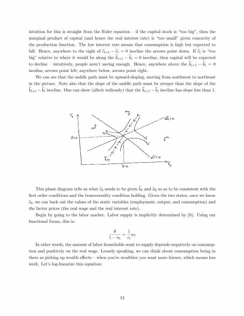
intuition for this is straight from the Euler equation – if the capital stock is “too big”, then the

marginal product of capital (and hence the real interest rate) is “too small” given concavity of

the production function. The low interest rate means that consumption is high but expected to

fall. Hence, anywhere to the right of ct+1 − ct = 0 isocline the arrows point down. If ct is “too

big” relative to where it would be along the kt+1 − kt = 0 isocline, then capital will be expected

to decline – intuitively, people aren’t saving enough. Hence, anywhere above the kt+1 − kt = 0

iscoline, arrows point left; anywhere below, arrows point right.

We can see that the saddle path must be upward-sloping, moving from southwest to northeast

in the picture. Note also that the slope of the saddle path must be steeper than the slope of the

kt+1− kt isocline. One can show (albeit tediously) that the kt+1− kt isocline has slope less than 1.

This phase diagram tells us what c0 needs to be given k0 and a0 so as to be consistent with the

first order conditions and the transversality condition holding. Given the two states, once we know

c0, we can back out the values of the static variables (employment, output, and consumption) and

the factor prices (the real wage and the real interest rate).

Begin by going to the labor market. Labor supply is implicitly determined by (6). Using our

functional forms, this is:

θ

1− nt=

1

ctwt

In other words, the amount of labor households want to supply depends negatively on consump-

tion and positively on the real wage. Loosely speaking, we can think about consumption being in

there as picking up wealth effects – when you’re wealthier you want more leisure, which means less

work. Let’s log-linearize this equation:

13

ln θ − ln(1− nt) = − ln ct + lnwt

−nt − n∗

1− n∗= −ct − c

∗

c∗+wt − w∗

w∗

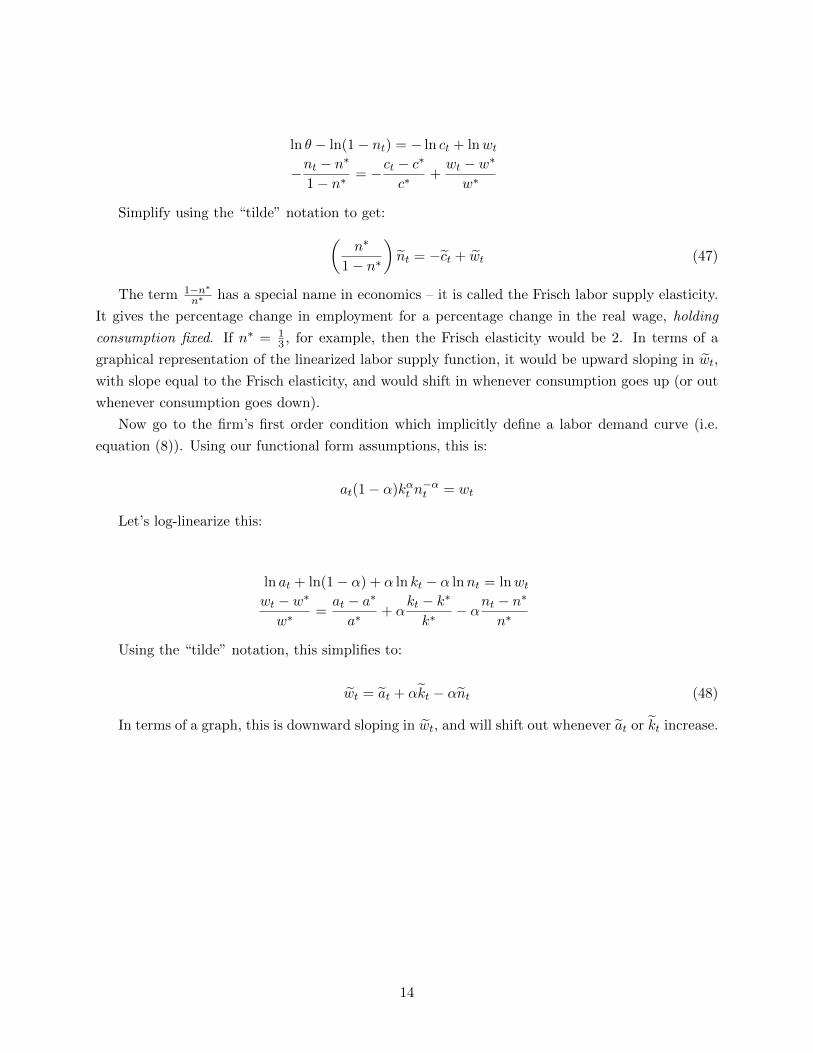
Simplify using the “tilde” notation to get:(n∗

1− n∗

)nt = −ct + wt (47)

The term 1−n∗n∗ has a special name in economics – it is called the Frisch labor supply elasticity.

It gives the percentage change in employment for a percentage change in the real wage, holding

consumption fixed. If n∗ = 13 , for example, then the Frisch elasticity would be 2. In terms of a

graphical representation of the linearized labor supply function, it would be upward sloping in wt,

with slope equal to the Frisch elasticity, and would shift in whenever consumption goes up (or out

whenever consumption goes down).

Now go to the firm’s first order condition which implicitly define a labor demand curve (i.e.

equation (8)). Using our functional form assumptions, this is:

at(1− α)kαt n−αt = wt

Let’s log-linearize this:

ln at + ln(1− α) + α ln kt − α lnnt = lnwtwt − w∗

w∗=at − a∗

a∗+ α

kt − k∗

k∗− αnt − n

∗

n∗

Using the “tilde” notation, this simplifies to:

wt = at + αkt − αnt (48)

In terms of a graph, this is downward sloping in wt, and will shift out whenever at or kt increase.

14

a0 and k0 are given. Once we know c0 from the phase diagram, we can determine the position

of the labor supply curve. The position of the labor demand curve is given once we know capital

and TFP. The intersection of the curves determines the real wage and level of employment.

Next we can determine output, given employment. Using our functional form assumptions,

yt = atkαt n

1−αt . Let’s log-linearize this:

ln yt = ln at + α ln kt + (1− α) lnntyt − y∗

y∗=at − a∗

a∗+ α

kt − k∗

k∗+ (1− α)

nt − n∗

n∗

Using the “tilde” notation, we get:

yt = at + αkt + (1− α)nt (49)

To figure out investment and the real interest rate, go to the condition for the optimal choice

of the future capital stock:

1

ct= βEt

(1

ct+1(αkα−1t+1 n

αt+1 + (1− δ))

)We know that the linearized version of this is given by (43). Linearize the expression for the

stochastic discount factor:

ln(1 + rt+1) = − lnβ + ln ct+1 − ln ct+1

Now linearize:

15

rt+1 − r∗ = Etct+1 − ct

Here I’m actually doing a double approximation, assuming that 1 + r∗ ≈ 0. When dealing with

variables that are already in percentage terms (e.g. interest rates), we just want the deviation from

steady state, not the percentage deviation from steady state (i.e. 0.05 is 0.01 percentage points

higher than 0.04, but 20 percent higher). Hence, define rt+1 = rt+1 − r∗. Then we have:

rt+1 = ct+1 − ct (50)

Substitute this into (43) to get:

rt+1 = βα

(k∗

n∗

)α−1Et

(at+1 + (α− 1)kt+1 + (1− α)nt+1

)So as to write this in terms of investment, look at the capital accumulation equation:

kt+1 = It + (1− δ)kt

Log-linearize this:

ln kt+1 = ln(It + (1− δ)kt)kt+1 − k∗

k∗=

1

k∗((It − I∗) + (1− δ)(kt − k∗))

Simplifying in terms of the “tilde” notation, and noting that I∗

k∗ = δ:

kt+1 = δIt + (1− δ)kt (51)

Now use this in (51) to write it in terms of investment:

rt+1 = βα

(k∗

n∗

)α−1 (at+1 − (1− α)δIt − (1− α)(1− δ)kt + (1− α)nt+1

)(52)

This says that investment demand is decreasing in the real interest rate, increasing in future

TFP, and increasing in future labor input. Graphically, the investment demand curve is downward

sloping.

In equilibrium, yt = ct + It. In log-linear form, we can solve for the equilibrium amount of

investment:

16

yt =c∗

y∗ct +

I∗

y∗It

It =y∗

I∗

(yt −

c∗

y∗ct

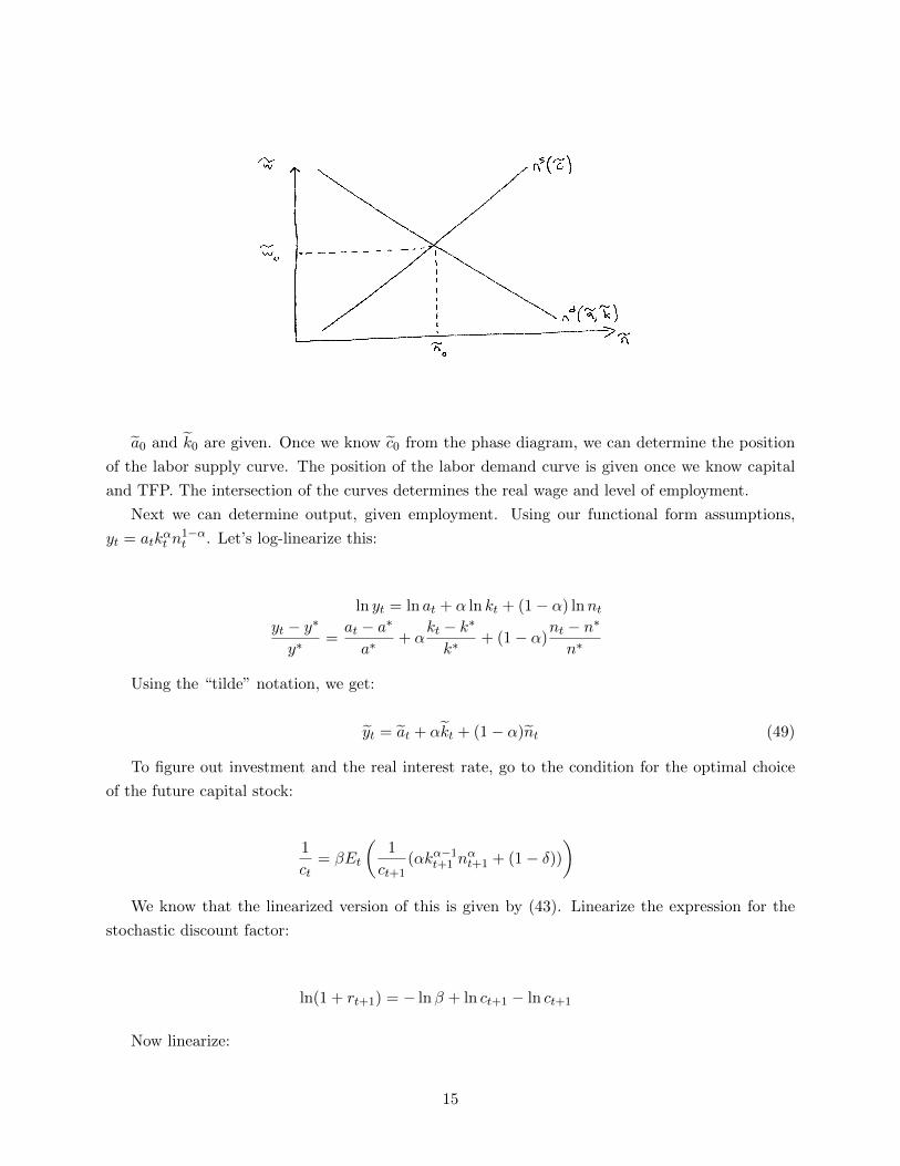
)Since we have already determined output and consumption, reading this point off of the invest-

ment demand curve determines the interest rate. See the figure below:

Hence, one can think about there being a “causal ordering”. Given TFP and capital, determine

consumption from the phase diagram. Given consumption, determine employment and the real

wage. Then given employment, determine output. Then given output and consumption, determine

investment and the real interest rate:

a0 & k0 → c0 → n0 & w0 → y0 → I0 & r1

4 Dynamic Analysis in Response to TFP Shocks

We want to qualitatively characterize the dynamic responses of the endogenous variables of the

model to shocks to TFP (the only source of stochastic variation in the model as it currently

stands).

Consider first an unexpected, permanent increase in at. This means we will end up in a new

steady state, which means that the new steady state of the linearized variables will not be zero,

as we linearized about the old steady state. From (46) and (47), we know that the two isoclines

must both shift “up” when a0 suddenly increases. The new isoclines must cross at a point with a

higher (relative to the initial) steady state capital and consumption (one can show this analytically).

17

There will also be a new saddle path associated with the “new” system. At time 0, consumption

must jump to the new saddle path, from which point it must be expected to “ride” it all the way

to the new steady state. The initial jump in consumption turns out to be ambiguous – it could

increase, decrease, or not change at all (similarly to the basic neoclassical case with fixed labor

input). That being said, for plausible parameterizations, consumption will jump up on impact

(permanent income intuition), and hence that’s how I’m going to draw it. See the phase diagram

below:

We can see from the picture that c jumps up on impact, from its initial steady state (with

c = 0), to c0. From thereafter it must ride the new saddle path to the new steady state, which in

terms of these linearized variables will feature k∗ > 0 and c∗ > 0, since we linearized about the

steady state associated with the old level of TFP.

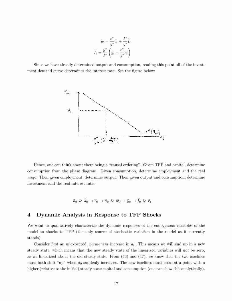
Now that we know consumption, go to the labor market. Higher TFP shifts labor demand

out. Higher consumption shifts labor supply in. The net effect is for the real wage to definitely be

higher, but there is an ambiguous effect on employment – it could go up, down, or not change at

all. I’m going to draw it as going up, as this seems to be the plausible case.

18

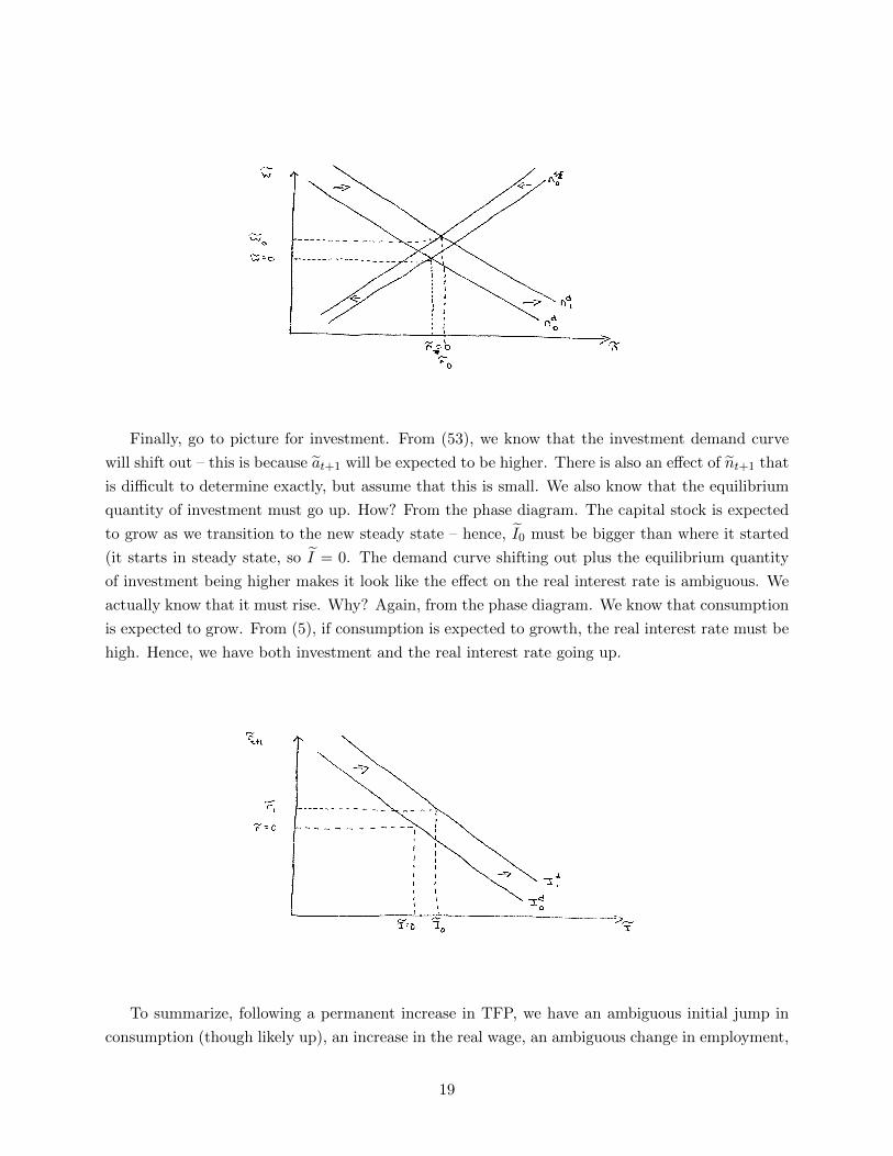
Finally, go to picture for investment. From (53), we know that the investment demand curve

will shift out – this is because at+1 will be expected to be higher. There is also an effect of nt+1 that

is difficult to determine exactly, but assume that this is small. We also know that the equilibrium

quantity of investment must go up. How? From the phase diagram. The capital stock is expected

to grow as we transition to the new steady state – hence, I0 must be bigger than where it started

(it starts in steady state, so I = 0. The demand curve shifting out plus the equilibrium quantity

of investment being higher makes it look like the effect on the real interest rate is ambiguous. We

actually know that it must rise. Why? Again, from the phase diagram. We know that consumption

is expected to grow. From (5), if consumption is expected to growth, the real interest rate must be

high. Hence, we have both investment and the real interest rate going up.

To summarize, following a permanent increase in TFP, we have an ambiguous initial jump in

consumption (though likely up), an increase in the real wage, an ambiguous change in employment,

19

an increase in output, an increase in investment, and an increase in the real interest rate. After

these impact effects, we follow the dynamics of the phase diagram. In particular, consumption and

the capital stock will grow (which means the real interest rate and investment will stay high). The

real wage will continue to grow – this is because, as consumption grows, the labor supply curve

will continue to shift in, and as capital grows, the labor demand curve will continue to shift out.

Employment will end up going back to its original steady state at some point – this is because the

expression for steady state employment is independent of a∗ (more on this later).

Next, consider a completely transitory increase in at. In other words, it only lasts today and

the expected value of at+1 is unchanged. In the phase diagram, this will approximately do nothing.

In reality consumption must jump a little, ride unstable dynamics for one period, and then end up

on the original saddle path, from which point it must be expected to return to its initial steady

state. Since the change is only “in effect” for a very short period of time, we can approximate the

jump in consumption as being zero. Thus, what approximately happens in the phase diagram is

nothing at all.

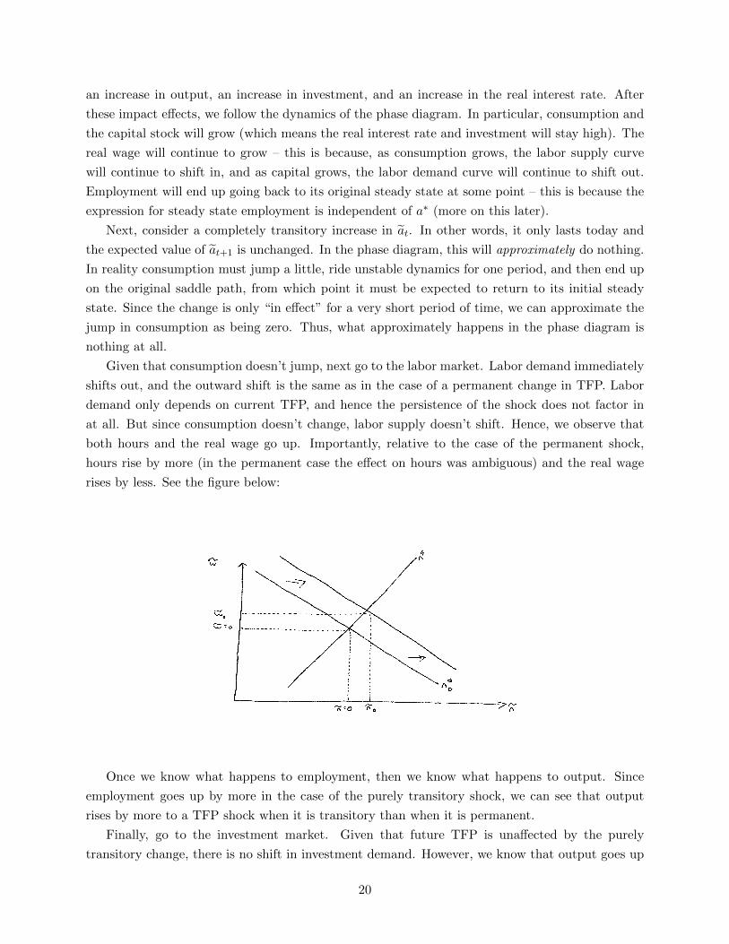
Given that consumption doesn’t jump, next go to the labor market. Labor demand immediately

shifts out, and the outward shift is the same as in the case of a permanent change in TFP. Labor

demand only depends on current TFP, and hence the persistence of the shock does not factor in

at all. But since consumption doesn’t change, labor supply doesn’t shift. Hence, we observe that

both hours and the real wage go up. Importantly, relative to the case of the permanent shock,

hours rise by more (in the permanent case the effect on hours was ambiguous) and the real wage

rises by less. See the figure below:

Once we know what happens to employment, then we know what happens to output. Since

employment goes up by more in the case of the purely transitory shock, we can see that output

rises by more to a TFP shock when it is transitory than when it is permanent.

Finally, go to the investment market. Given that future TFP is unaffected by the purely

transitory change, there is no shift in investment demand. However, we know that output goes up

20

and consumption doesn’t change. This means that the quantity of investment today must increase.

Furthermore, it must increase by more than it does in the case of a permanent change in TFP.

We know this because output increases by more when the change in transitory and consumption

increases by less – thus the difference goes up by more. Going to the figure, this must mean that

the real interest rate falls. See below:

The two cases thus far considered are somewhat knife edge. Most of the time we are interested

in looking at what happens in response to persistent – but transitory – shocks. The above exercises

are helpful because they provided “bounding results”. The more persistent the shock is (e.g. the

bigger is ρ), the more the results look like the permanent case. The less persistent the shock (e.g.

the smaller is ρ), the more the results like the purely transitory case.

We can thus make the following qualitative statements that can be verified quantitatively by

numerically solving the model:

1. The more persistent the increase in TFP, the more consumption increases on impact (or falls

by less). In the limiting case where the change in TFP is just one period, consumption will

approximately not react.

2. The more persistent the increase in TFP, the less hours react and the more real wages increase.

3. The more persistent the increase in TFP, the less output reacts

4. The more persistent the increase in TFP, the less investment reacts and the real interest rate

increases by more (or falls by less).

21