graph optimization using fractal decomposition
TRANSCRIPT
GRAPH OPTIMIZATION USING FRACTAL DECOMPOSITION
JAMES R. RIEHL AND JOAO P. HESPANHA†
Abstract. We introduce a method of hierarchically decomposing graph optimization problemsto obtain approximate solutions with low computation. The method uses a partition on the graphto convert the original problem to a high level problem and several lower level problems. On eachlevel, the resulting problems are in exactly the same form as the original one, so they can be furtherdecomposed. In this way, the problems become fractal in nature. We use best-case and worst-case instances of the decomposed problems to establish upper and lower bounds on the optimalcriteria, and these bounds are achieved with significantly less computation than what is requiredto solve the original problem. We show that as the number of hierarchical levels increases, thecomputational complexity approaches O(n) at the expense of looser bounds on the optimal solution.We demonstrate this method on three example problems: all-pairs shortest path, all-pairs maximumflow, and cooperative search. Large-scale simulations show that this fractal decomposition methodis computationally fast and can yield good results for practical problems.
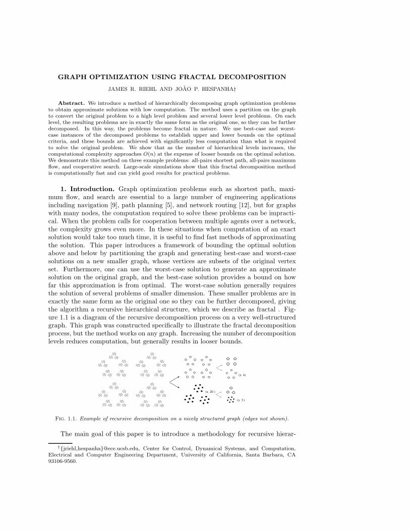
1. Introduction. Graph optimization problems such as shortest path, maxi-mum flow, and search are essential to a large number of engineering applicationsincluding navigation [9], path planning [5], and network routing [12], but for graphswith many nodes, the computation required to solve these problems can be impracti-cal. When the problem calls for cooperation between multiple agents over a network,the complexity grows even more. In these situations when computation of an exactsolution would take too much time, it is useful to find fast methods of approximatingthe solution. This paper introduces a framework of bounding the optimal solutionabove and below by partitioning the graph and generating best-case and worst-casesolutions on a new smaller graph, whose vertices are subsets of the original vertexset. Furthermore, one can use the worst-case solution to generate an approximatesolution on the original graph, and the best-case solution provides a bound on howfar this approximation is from optimal. The worst-case solution generally requiresthe solution of several problems of smaller dimension. These smaller problems are inexactly the same form as the original one so they can be further decomposed, givingthe algorithm a recursive hierarchical structure, which we describe as fractal . Fig-ure 1.1 is a diagram of the recursive decomposition process on a very well-structuredgraph. This graph was constructed specifically to illustrate the fractal decompositionprocess, but the method works on any graph. Increasing the number of decompositionlevels reduces computation, but generally results in looser bounds.
(x 20 )
(x 4)
(x 3 )
Fig. 1.1. Example of recursive decomposition on a nicely structured graph (edges not shown).
The main goal of this paper is to introduce a methodology for recursive hierar-
†{jriehl,hespanha}@ece.ucsb.edu, Center for Control, Dynamical Systems, and Computation,Electrical and Computer Engineering Department, University of California, Santa Barbara, CA93106-9560.
chical decomposition of graph optimization problems and to implement it on threewell-known and practical problems. We will show that this fractal decompositionalgorithm greatly reduces computation, and as the number of decomposition levelsincreases, the computational complexity approaches O(n). Furthermore, for each ofthe three examples, we provide numerical simulations to demonstrate that the ap-proximation can be quite accurate. First, we introduce the three problems along withprevious computational complexity results.
• Shortest path matrix. The shortest path matrix problem, also called all-pairs shortest paths, involves finding the minimum-cost path between everypair of vertices in a graph. There are a great number of applications of thisproblem, including optimal route planning for groups of UAVs [11]. For aweighted directed graph with n vertices and m edges, Karger et al. showedthat the all-pairs shortest path problem can be solved with computationalcomplexity O(nm + n2 log n) [10].
• Maximum flow matrix. The maximum flow matrix problem involves find-ing the flow assigment on the edges of a capacitated graph that yields themaximum flow intensity between every pair of vertices. Applications of thisproblem include stochastic network routing [1] and vehicle routing [2]. Givena directed graph G(V, E) with n vertices and m capacitated edges, Goldbergand Tarjan [6] showed that one can compute the maximum flow between two
vertices in O(nm log n2
m) time. To compute the max-flow between all pairs
of vertices in an undirected graph, Gomory and Hu showed that one onlyneeds to solve n−1 maximum flow problems [7], but since we are considering
directed graphs, we must compute the flow between all n(n−1)2 vertices. This
results in a complexity of O(n3m log n2
m) to generate the complete max-flow
matrix.• Cooperative graph search. The objective of the cooperative graph search
problem is to find paths in a graph that maximize the probability that a teamof cooperating agents will find a hidden target, subject to a cost constraint onthe paths. The computational complexity of the search problem for a singleagent is known to be NP-Hard [17] on the number of vertices n. Reducing thes-agent cooperative search problem to a single-agent search problem with ns
vertices results in a problem that is clearly also NP-Hard. In the worst case,an exhaustive search on a complete graph would have complexity O(ns!).Although there are some more efficient algorithms to solve this problem suchas the branch and bound methods of Eagle and Yee [4], this problem is stillcomputationally infeasible for large values of ns.
There is some previous literature on hierarchical decomposition applied to variousgraph optimization problems, most prevalently the shortest path problem. Romeijnand Smith proposed an algorithm to solve an aggregated all-pairs shortest path prob-lem motivated by minimizing vehicle travel time [14]. Under the assumption thatgraphs in each level of aggregation have the same structure, they showed the compu-tational complexity of their approximation (using parallel processors) to be O(n log n)
for aggregation on two levels of sparse graphs, and O(n2L log n) for aggregation on L
levels. The results of our shortest path decomposition example will closely resem-ble that of [14] with the addition of both upper and lower bounds on the costs ofthe shortest paths. Also related, Shen and Caines presented results on hierarchicallyaccelerated dynamic programming [15]. Using state aggregation methods, they were

able to speed up dynamic programming algorithms for finite state machines by ordersof magnitude at the expense of some sub-optimality, for which they give bounds.
Towards approximating the maximum flow problem, Lim et al. developed atechnique to compute routing tables for stochastic network routing that involves atwo-level hierarchical decomposition of the network. They reduced computationalcomplexity from O(n5) to O(n3.1) with a performance that is in some cases as goodas the general flat max-flow routing problem [12]. Our maximim flow decompositionimproves the two-level computational complexity to O(n3) and adds the capability todecompose on more levels using the fractal framework.
DasGupta et al. presented an approximate solution for the stationary targetsearch based on an aggregation of the search space using a graph partition [3]. Weused a similar approach in [13] while also allowing the partitioning process to beimplemented on multiple levels.
The remainder of this paper is organized as follows. Section 2 presents the ideaof partitions and metagraphs, introducing concepts and notation that will be usedthroughout the paper. Section 3 gives an abstract overview of the fractal decomposi-tion methodology, with generic computation results presented in section 4. Sections5, 6, and 7 define three example problems and give procedures to construct upperand lower bounds on the optimal criteria. These sections also include explicit proce-dures for constructing the approximate shortest path matrix, maximum flow matrix,and cooperative search paths. We include brief numerical examples for shortest pathand maximum flow, and a more extensive simulation study on the cooperative searchproblem. The final section is a discussion of the results with suggestions for futureresearch.
2. Graphs, Metagraphs, and Subgraphs. This section introduces some no-tation and terminology that we will use in the remainder of this paper. Given a graphG := (V, E) with vertex set V and edge set E ⊂ V ×V , a partition V := {v1, v2, . . . , vk}of G is a set of disjoint subsets of V such that v1 ∩ v2 ∩ . . . ∩ vk = V . We call thesesubsets vi metavertices. For a given metavertex vi ∈ V , we define the subgraph of Ginduced by vi to be the subgraph G|vi := (vi, E ∩ vi × vi).
v3
v4
G
v2
v1
G
G|v1G|v2
G|v3G|v4
Fig. 2.1. Example of a graph partitioned into 4 metavertices.
Figure 2.1 shows an example of the graph partitioning process, where the dashedlines through G separate the partitioned subgraphs G|vi, which are represented bymetavertices in G.
Given a partition V of the vertex set V , we define the metagraph of G induced by
the partition V to be the graph G := (V , E) with an edge e ∈ E between metavertices
vi, vj ∈ V if and only if G has at least one edge between vertices v and v′ for somev ∈ vi and v′ ∈ vj . In general, there may exist several such edges e ∈ E and we callthese the edges associated with the metaedge e.

3. Fractal Decomposition Method. We now describe a methodology forbounding and approximating the solution to a graph optimization problem usingfractal decomposition. The ideas presented here will be applied to several exampleproblems in the following sections. The steps of the fractal decomposition method arelisted below.
1. Partition the graph2. Construct bounding metaproblems and solve3. Refine worst-case solution to approximate solution on original graph
3.1. Partition the graph. Although the algorithm will work for any partition,some partitions will result in tighter bounds than others, and some will reduce compu-tation more than others. These factors will depend on the specific problem and shouldbe taken into account in the choice of partitioning algorithm. In general, the first ob-jective of the graph partition is to decompose the problem such that the differencebetween upper and lower bounds is small. For example, in the shortest path problem,this means grouping vertices that are connected by low-cost edges whereas in the max-imum flow problem, this means grouping vertices connected by high-bandwidth edges.The partitioning algorithm we use is the one in [8], which tries to minimize the totalcost of cut edges by clustering the eigenvectors of a (doubly stochastic) modificationof the adjacency matrix around the k most linearly independent eigenvectors.
3.2. Construct bounding metaproblems and solve. We now want to con-struct two metagraphs using the results of the graph partition: a worst-case meta-graph and a best-case metagraph. Both metagraphs share the metavertex set andmetaedge set defined by the partition. Optimization problems on the metagraphsare called metaproblems. The metaproblems should be in the exact same form as theoriginal problem, so that we may apply any algorithm that solves the original problemto the metaproblems. This property allows for recursive decomposition. The mostimportant step in the construction is assigning data (costs, rewards, bandwidths,etc.) to the metavertices and metaedges such that the solutions to the metaprob-lems are guaranteed to bound the solution to the original problem. For the bestcase metaproblem, this step just means assigning the most optimistic values. Forthe worst-case metaproblem, this step generally involves assigning the solution toa smaller problem, defined on the subgraph associated with the metavertex, to themetavertices, and giving a pessimistic assignment to the metaedges. The solution tothe worst-case metaproblem will yield the conservative bound and will facilitate theconstruction of an approximate solution on the original graph. The solution to thebest-case metaproblem will tell us how far our approximate solution is from optimal.
3.3. Refine worst-case solution to approximate solution on original
graph. As mentioned above, the solution to the worst-case metaproblem will in-volve solving a set of smaller subproblems. The approximate solution is generated bya refinement process on the worst-case metagraph, using the solutions to these sub-problems, to generate a feasible solution on the original graph. This is made possiblebecause the worst-case metaproblem is formulated in such a way that the resultingapproximation is guaranteed to be feasible.
4. Computational Complexity. For the purposes of this analysis, let f(n, k)denote the computational complexity of a given graph optimization problem on nvertices decomposed into k metavertices. Without decomposition, the complexity isf(n, 1). Now, let us see what happens with one level of decomposition. Suppose thatwe partition the graph into k subgraphs each containing roughly n
kvertices. The
computational complexity of the worst-case decomposed problem is then
f(n, k) = f(k, 1) + kf(n
k, 1), (4.1)
where the first term comes from solving a problem on the metagraph, and the secondterm comes from solving problems on the k subgraphs. Decomposing on a secondlevel yields
f(n, k0) = f(k0, k1) + k0f(n
k0, k2)
= f(k1, 1) + k1f(k0
k1, 1)
+ k0f(k2, 1) + k0k2f(n
k0k2, 1). (4.2)
A choice of k =√
n in (4.1) makes the computation of the upper-level meta problemequal to that of the k subproblems. For two levels, the analogous choices are k0 =
√n,
and k1 = k2 =√
k0 = 4√
n. Continuing the recursive decomposition in this mannergives the following computational complexity results:
Level 0 : f(n, 1)
Level 1 : (√
n + 1)f(√
n, 1)
Level 2 : (√
n + 1)( 4√
n + 1)f( 4√
n, 1)
...
Level L :
2L−1∑
i=0
ni
2L f(n1
2L , 1)
=
(
n − 1
n1
2L − 1
)
f(n1
2L , 1).
We can limit the number of decomposition levels to Lmax = ⌊log2(log2(n))⌋ becausethere is no advantage to decomposing a graph with only two vertices. It followsthat as L approaches this maximum value, the computational complexity approaches(n − 1)f(2, 1), which is equivalent to O(n) since f(2, 1) is a constant. Hence, as thenumber of decomposition levels increases, the complexity approaches linearity.
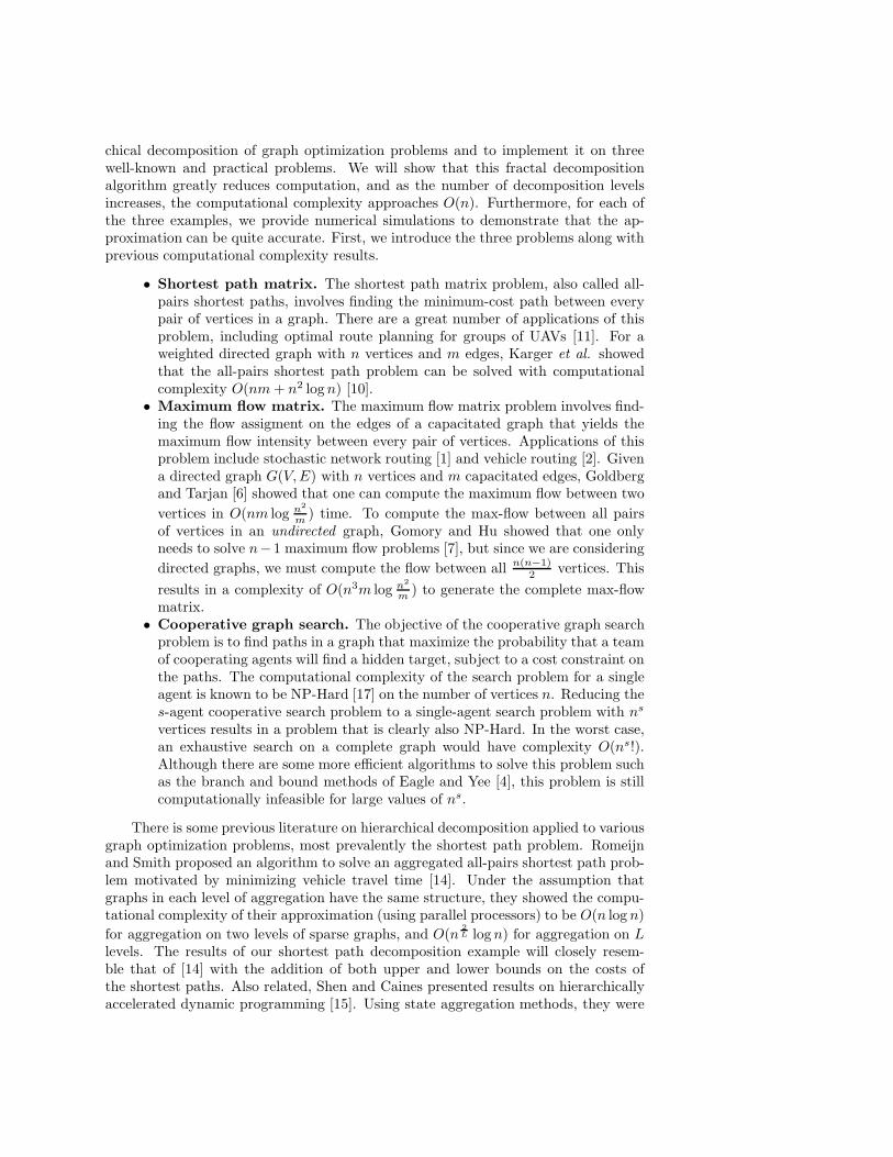
Inherent to this analysis is the assumption that the computational complexity ofa given problem can be expressed solely as a function of the number of vertices inthe graph. This is not generally the case because the complexity of many algorithmsalso depends on the number of edges m. However, we can obtain an upper boundon the computational complexity by analyzing the results for dense graphs, whereO(m) = O(n2). Similarly, setting O(m) = O(n) yields the best-case complexityfor sparse graphs. Table 4.1 shows the computational reduction for various levels ofdecomposition on the three problems presented in this paper.
In the cooperative search column, s is the number of searchers, and the com-plexities listed are for an exhaustive search. For this analysis, we assume that thecomplexity associated with graph partitioning is negligable compared to that of theoptimization problem, which may or may not be the case depending on the specificpartitioning algorithm used.
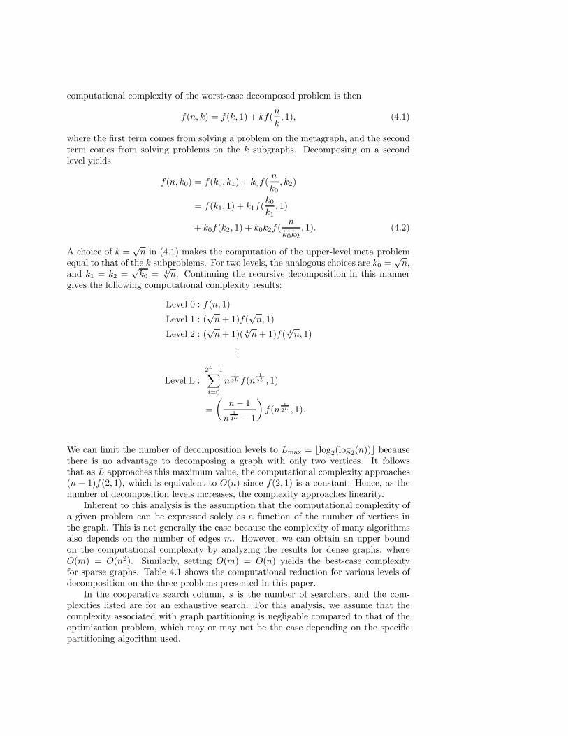
Table 4.1
Computational Complexity of Worst-Case Metaproblems for up to 3 Decomposition Levels onDense Graphs
Levels Shortest Path Matrix Maximum Flow Matrix Cooperative Search
0 O(n3) O(n5) O(ns!)
1 O(n2) O(n3) O(n12 (n
s2 )!)
2 O(n32 ) O(n2) O(n
34 (n
s4 )!)
3 O(n54 ) O(n
32 ) O(n
78 (n
s8 )!)
5. Shortest Path Matrix Problem. The shortest path matrix problem in-volves constructing a n × n matrix of the minimum-cost path between all pairs ofvertices in a graph. Our formulation is a slight variation on the conventional APSPproblem because in addition to assigning a cost to each edge, we also assign a costto each vertex. This is crucial in facilitating the hierarchical decomposition of theproblem, as will be explained in section 5.1. Adding vertex costs does not increasethe computational complexity of the problem.
Data
G := (V, E) directed graph
ce : E → [0,∞) edge cost function
cv : V × O → [0,∞) vertex cost function
Path A path in G from vinit ∈ V to vfinal ∈ V is a sequence of vertices (wherev1 := vinit, vf := vfinal)
p := (v1, v2, . . . , vf−1, vf ), (vi, vi+1) ∈ E.
The path-cost is given by
C(p) :=
f−1∑
i=1
ce(vi, vi+1) +
f∑
i=1
cv(vi).
Objective For every pair of vertices (vinit, vfinal), compute the path p that mini-mizes the path-cost C(p). We denote this path by p∗ and the minimum cost C(p∗)by J∗
G(vinit, vfinal). The largest minimum cost over all possible pairs of vertices(vinit, vfinal) is called the diameter of the graph and is denoted by ‖G‖.
5.1. Worst-case meta-shortest path. Let Gworst := (V , E) be a metagraphof G, with edge cost and vertex cost defined by
ceworst(e) := mine∈e
η(e) cvworst(v) :=∥
∥G|v∥
∥.
Note that to assign the vertex costs of Gworst one needs to compute the diameterof all subgraphs and therefore solve k smaller shortest-path matrix problems. This isthe key step in the hierarchical decomposition of the problem.
5.2. Best-case meta-shortest path. Let Gbest := (V , E) be a metagraph ofG, with edge cost and vertex cost defined by
cebest(e) := min
e∈ece(e) cvbest
(v) := minv∈v
ν(v).
Theorem 1 For every partition V of G
J∗Gbest
(vinit, vfinal) ≤ J∗G(vinit, vfinal) ≤ J∗
Gworst(vinit, vfinal) (5.1)
where vinit ∈ vinit, vfinal ∈ vfinal.
The construction of the upper bound provides a procedure for generating anapproximate shortest path between each pair of vertices in G, and the cost of thispath lies between J∗
G(vinit, vfinal) and J∗Gworst
(vinit, vfinal).
Proof. To verify the upper bound, we will show that one can easily use theshortest path from vinit to vfinal in Gworst to construct an approximate shortest pathfrom vinit to vfinal in G. We do this by sequentially connecting vinit, the endpoints ofthe minimum cost edge between each metavertex in the optimal worst-case path, andvfinal with the shortest path between them in G. The detailed procedure is describedbelow.
Let p∗w be the shortest path from vinit to vfinal in Gworst, and p be the approximateshortest path in G being constructed. To begin, we want p to include the minimumcost edge of each metaedge in p∗w. Call this set of edges E∗
w. From the set of verticesadjacent to these edges, let vjexit
be the exit vertex of vj , that is, the vertex invj adjacent to the edge in E∗
worst associated with the metaedge that connects vj
to vj+1 for j = (1, 2, . . . , f − 1), and let vjentrybe the entry vertex of each vj for
j = (2, 3, . . . , f). The incomplete path is then
p = (vinit, . . . , vexit1 , . . . , ventry2, . . . , vexit2 , . . .
. . . , vexitf−1, . . . , ventryf
, . . . , vfinal).
Now, simply fill in the gaps with the shortest path between the surrounding nodes.Recall that we already computed the shortest paths between all pairs of vertices ina metavertex when we found the diameter of each subgraph G|vj , so this data isavailable without additional computation.
Let pj denote the portion of the path p contained within the metavertex vj . Wecan now compare the costs of the two paths p and p∗w:
C(p∗w) =
f−1∑
j=1
ceworst(vj , vj+1) +
f∑
j=1
∥
∥G|vj
∥
∥ (5.2)
C(p) =
f−1∑
j=1
ceworst(vj , vj+1) +
f∑
j=1
C(pj) (5.3)
Because we have defined each pj to be a shortest path between two nodes in vj ,the cost of this path C(pj) must be no greater than
∥
∥G|vj
∥
∥. Summing over the sameset of metavertices, the last term of (5.3) must be less than or equal to the last termof (5.2). Since the edge cost terms are identical, we conclude that

C(p∗) ≤ C(p) ≤ C(p∗w), (5.4)
where p∗ is the shortest path in G from vinit to vfinal. The left inequality in (5.4)holds because of the optimality of p∗, and the right inequality was discussed above.Therefore, the upper bound in (5.1) holds.
We now check the lower bound by constructing a feasible path from vinit to vfinal
in Gbest from the optimal path p∗ connecting vinit to vfinal in G.The constructed path, which we will call pb, will consist of the sequence of
metavertices that contain vertices of p∗ in order but with no consecutive repetitions.We can construct this path by first setting pbest = p∗ and then replacing each vertexvi with the metavertex vj in which it is contained. Deleting all repeated metaverticesyields the desired path pbest = (v1, v2, . . . , vf ), where f is the length of pbest.
Let Ep∗ denote the set of edges along the path p∗. Define Ep∗
jas the set of these
edges having both endpoints in vj , and Ep∗ as the set of all edges totally containedwithin metavertices, for j ∈ [1, f ]. The remaining edges connecting consecutive vj
along p∗ are contained in the set difference Ep∗
j:= Ep∗\Ep∗ .
We can express the cost of the two paths as follows:
C(pb) =
f−1∑
j=1
cebest(vj , vj+1) +
f∑
j=1
cvbest(vj) (5.5)
C(p∗) =∑
e∈Ep∗
ce(e) +∑
e∈Ep∗
ce(e) +
f∑
i=1
ν(vi), (5.6)
where f is the length of p∗.The first term on the right side of (5.6) is the cost of the edges in p∗ between
metavertices and this is definitely greater than or equal to the sum of the minimumedge costs between the same sequence of metavertices, which is the first term on theright side of (5.5). Using this and the trivial fact that the sum of the minimum vertexcosts in each metavertex, which is the second term on the right of (5.5), is less thanor equal to the sum of total costs incurred by p∗ within metavertices, the second andthird terms on the right of (5.6), we see that the lower bound in 5.1 indeed holds.
5.3. Error Bounds for Simple Graphs. The approximation bounds discussedthus far are problem dependent, that is, varying the graph, graph data, or partitionwill also vary the resulting bounds. A natural question to ask is whether it is possibleto guarantee bounds that do not depend on the particular instance of the problem.While this is quite a difficult problem for arbitrary graphs, we can generate con-stant factor approximation bounds for some simple, highly structured graphs, such aslattices.
To begin, let us consider the shortest-path problem on a two-dimensional rect-angular lattice graph, where each of the edge costs is 1, and all the vertex costs are0. For simplicity of the partition, we look at square lattices of size n = i2 × i2,where i ∈ N. The diameter of such a graph is 2(n
12 − 1). Now, we apply one level
of decomposition to the problem, dividing the graph into n12 blocks each having n
12
vertices, and construct the worst-case metagraph. The diameter of this metagraph is4(n
12 − n
14 ). The ratio of these diameters is
∣
∣
∣
∣Gworst(n)∣
∣
∣
∣
||G(n)|| =4(n
12 − n
14 )
2(n12 − 1)
=2n
14
n14 + 1
Taking the limit as n → ∞ above, we obtain the following constant factor approxi-mation result:
∣
∣
∣
∣Gworst(n)∣
∣
∣
∣ ≤ 2 ||G(n)|| .
It is straightforward to show that the approximation factor is 4 for two levels ofdecomposition, 8 for three, and 2L for L.
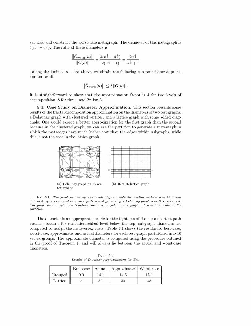
5.4. Case Study on Diameter Approximation. This section presents someresults of the fractal decomposition approximation on the diameters of two test graphs:a Delaunay graph with clustered vertices, and a lattice graph with some added diag-onals. One would expect a better approximation for the first graph than the secondbecause in the clustered graph, we can use the partition to generate a metagraph inwhich the metaedges have much higher cost than the edges within subgraphs, whilethis is not the case in the lattice graph.
(a) Delaunay graph on 16 ver-tex groups
(b) 16 × 16 lattice graph.
Fig. 5.1. The graph on the left was created by randomly distributing vertices over 16 1 unit× 1 unit regions centered in a block pattern and generating a Delaunay graph over this vertex set.The graph on the right is a two-dimensional rectangular lattice graph. Dashed lines indicate thepartition.
The diameter is an appropriate metric for the tightness of the meta-shortest pathbounds, because for each hierarchical level below the top, subgraph diameters arecomputed to assign the metavertex costs. Table 5.1 shows the results for best-case,worst-case, approximate, and actual diameters for each test graph partitioned into 16vertex groups. The approximate diameter is computed using the procedure outlinedin the proof of Theorem 1, and will always lie between the actual and worst-casediameters.
Table 5.1
Results of Diameter Approximation for Test
Best-case Actual Approximate Worst-case
Grouped 9.0 14.1 14.5 15.1
Lattice 5 30 30 48
As expected, the worst-case bounds are fairly tight for the clustered graph, butworse for the lattice graph. The worst-case metagraph diameter of 48 lies withinthe constant factor bound of 2 derived in section 5.3. Although the approximationis exact for the lattice graph, there is a large uncertainty due to the best-case lowerbound. We conclude that using fractal decomposition to approximate the shortestpath matrix problem works best on graph with some inherent clustered structure.
6. Maximum Flow Matrix Problem. In the maximum flow matrix problem,the goal is to construct an n × n matrix containing the maximum flow intensitiesbetween all pairs of vertices in a graph. The flow through each edge is limited by thebandwidth or capacity of that edge. In this formulation, the vertices are also assignedbandwidths. The vertex bandwidth is what allows for the hierarchical decompositionof this problem.
Data
G := (V, E) directed graph
be : E → [0,∞) edge bandwidth function
bv : V × O → [0,∞) vertex bandwidth function
Flow A flow in G from vinit ∈ V to vfinal ∈ V is a function f : E → [0,∞) for whichthere exist some µ ≥ 0 such that
fout(v) − fin(v) =
µ v = vinit
−µ v = vfinal
0 otherwise,
∀v ∈ V, (6.1)
0 ≤ f(e) ≤ be(e), ∀e ∈ E (6.2)
0 ≤ fin(v) ≤ ν(v), ∀v ∈ V (6.3)
0 ≤ fout(v) ≤ ν(v), ∀v ∈ V (6.4)
In the above,
fin(v) :=∑
e∈In[v]
f(e), fout(v) :=∑
e∈Out[v]
f(e), (6.5)
where In[v] denotes the set of edges that enter the vertex v and Out[v] the set of edgesthat exit v. The constant µ is called the intensity of the flow.
Objective For every pair of vertexes (vinit, vfinal), compute the flow f∗ with maxi-mum intensity µ from vinit to vfinal. The maximum intensity is denoted by J∗
G(vinit, vfinal)and is called the maximum flow from vinit to vfinal. The smallest maximum flow overall possible pairs of vertices is called the bandwidth of the graph and is denoted by‖G‖.
6.1. Worst-case meta-max flow. Let Gworst := (V , E) be a metagraph of G,with edge bandwidth and vertex bandwidth defined by
beworst(e) :=∑
e∈e
be(e) bvworst(v) :=∥
∥G|v∥
∥. (6.6)
Note that to construct the graph Gworst one needs to compute the bandwidth ofall subgraphs and therefore solve several smaller max-flow matrix problems.
6.2. Best-case meta-max flow. Let Gbest := (V , E) be a metagraph of G,with edge bandwidth and vertex bandwidth defined by
bebest(e) :=∑
e∈e
be(e) bvbest(v) := +∞. (6.7)
Theorem 2 For every partition V of G
J∗Gworst
(vinit, vfinal) ≤ J∗G(vinit, vfinal) ≤ J∗
Gbest(vinit, vfinal)
where vinit ∈ vinit, vfinal ∈ vfinal.
In the proof of Theorem 2, the construction of the lower bound contains a pro-cedure for generating an approximate maximum flow between each pair of vertices inG, and the intensity of this flow lies between J∗
Gworst(vinit, vfinal) and J∗
G(vinit, vfinal).
To verify the lower bound, the idea is to construct a flow f(e) in G that satisfies(6.1)–(6.4) out of the worst-case maximum flow f∗
worst(e) in Gworst. This is possiblebecause the subgraphs associated with each metavertex are connected and the totalflow into and out of a metavertex is always no greater than the bandwidth of thatmetavertex. The intensity of this approximate maximum flow is bounded below byJ∗
Gworst(vinit, vfinal), and above by J∗
G(vinit, vfinal).
Proof. Let fw(e) be the maximum flow assignment of Gworst. Out of fw(e), wenow construct a flow f(e) in G that satisfies (6.1)–(6.4).
For every e ∈ E, decompose the flow in the worst-case metagraph as a flow in theoriginal graph as follows:
fw(e) = f(e1) + f(e2) + · · · + f(ep), (6.8)
where the notation ei is used to index the edges associated with the metaedge e, andp is the total number of these edges.
Since (6.2) holds for the worst-case metagraph, that is
0 ≤ f∗w(e) ≤ beworst(e) =
∑
e∈e
be(e),
we know that a decomposition (6.8) exists whose flows satisfy condition (6.2) for theoriginal graph.
Now we have assigned flows to the subset of edges of G that connect metaverticesof Gworst, but we still have to consider the edges of G that lie inside metavertices.
For every v ∈ V , there exist sets v′in and v′out defined by
v′in = {v ∈ v : (u, v) ∈ E, u /∈ v, v ∈ v} ∪ ({vinit} ∩ v)
v′out = {v ∈ v : (u, v) ∈ E, u ∈ v, v /∈ v} ∪ ({vfinal} ∩ v)
The set vin consists of all vertices in v to which an edge originating outside themetavertex is directed, plus the source vertex if v = vinit. Similarly, the set vout con-sists of all vertices in v from which an edge directed outside the metavertex originates,plus the sink vertex if v = vfinal. Some vertices may be contained in both vin andvout. To separate these vertices, we define the following disjoint sets:
vin ={
v ∈ v′in : fin(v) − fout(v) > 0}
vout ={
v ∈ v′out : fin(v) − fout(v) < 0}
,
where fin and fout are as defined in (6.5). Recall that we have only assigned f(e) toedges connecting metavertices. For all other edges, f(e) is temporarily set to zero.
We can now define a set of k subproblems, one for each v ∈ V , where the goal isto find a feasible flow from vin to vout.
The following procedure will find such a flow. For simplicity, assume that floworiginating at the source vinit is an inflow, and the flow terminating at the sink vfinal
is an outflow.
1. Enumerate the sets vin ={
vin1, vin2
, . . . , vinp
}
and vout ={
vout1 , vout2 , . . . , voutq
}
2. Initially, i = 1 and j = 1.3. Since each subgraph G|v is connected, there exists at least one path from
vinito voutj
. Assign the flow along one such path to be the minimum of theflow into vini
and the flow out of voutj. Subtract this value from the flow
intensities of both vertices.4. If i = p and j = q then stop. The procedure is complete.5. If the flow into vini
is still greater than the flow out, repeat step 3 for vini
and voutj+1. Otherwise execute step 3 for vini+1
and voutj.
By construction, assigning flows in this manner preserves condition (6.1) becauseat the end of the procedure the net flow is zero at all vertices excluding vinit and vfinal,for which it is µ and −µ, respectively. Also, since the flow through a metavertex vis bounded above by the bandwidth of the subgraph G|v, the flows generated by thisprocedure will satisfy (6.2)-(6.4).
This completes our construction of a feasible flow f(e) in the original graph basedon the worst-case flow f∗
w(e) in the metagraph. Therefore,
J∗G(vinit, vfinal) ≥ J∗
Gworst(vinit, vfinal). (6.9)
The proof for the best-case upper bound is straightforward because we can easilyconstruct a flow in Gbest from an optimal flow f∗(e) in G.
Let fbest(e) be a not necessarily optimal flow in Gbest, where
fbest(e) =∑
e∈e
f∗(e)
Since we know that f∗(e) satisfies (6.1) and (6.2), it follows from (6.7) and the
above equation that fbest(e) satisfies (6.1) and (6.2). Since bvbest(v) = ∞, (6.3) and(6.4) hold also.
Let JGbest(vinit, vfinal) be the intensity of the flow fbest(e).
As expected,
J∗Gbest
(vinit, vfinal) ≥ JGbest(vinit, vfinal) = J∗
G(vinit, vfinal)
The equality on the right holds from our construction of fbest(e). The inequalityon the left holds by definition of optimality. This result combined with (6.9) provesTheorem 2.
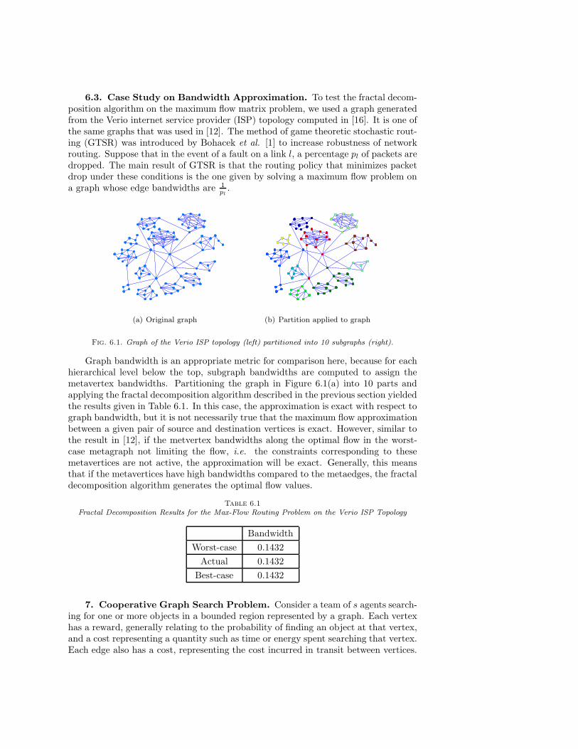
6.3. Case Study on Bandwidth Approximation. To test the fractal decom-position algorithm on the maximum flow matrix problem, we used a graph generatedfrom the Verio internet service provider (ISP) topology computed in [16]. It is one ofthe same graphs that was used in [12]. The method of game theoretic stochastic rout-ing (GTSR) was introduced by Bohacek et al. [1] to increase robustness of networkrouting. Suppose that in the event of a fault on a link l, a percentage pl of packets aredropped. The main result of GTSR is that the routing policy that minimizes packetdrop under these conditions is the one given by solving a maximum flow problem ona graph whose edge bandwidths are 1
pl.
(a) Original graph (b) Partition applied to graph
Fig. 6.1. Graph of the Verio ISP topology (left) partitioned into 10 subgraphs (right).
Graph bandwidth is an appropriate metric for comparison here, because for eachhierarchical level below the top, subgraph bandwidths are computed to assign themetavertex bandwidths. Partitioning the graph in Figure 6.1(a) into 10 parts andapplying the fractal decomposition algorithm described in the previous section yieldedthe results given in Table 6.1. In this case, the approximation is exact with respect tograph bandwidth, but it is not necessarily true that the maximum flow approximationbetween a given pair of source and destination vertices is exact. However, similar tothe result in [12], if the metvertex bandwidths along the optimal flow in the worst-case metagraph not limiting the flow, i.e. the constraints corresponding to thesemetavertices are not active, the approximation will be exact. Generally, this meansthat if the metavertices have high bandwidths compared to the metaedges, the fractaldecomposition algorithm generates the optimal flow values.
Table 6.1
Fractal Decomposition Results for the Max-Flow Routing Problem on the Verio ISP Topology
Bandwidth
Worst-case 0.1432
Actual 0.1432
Best-case 0.1432
7. Cooperative Graph Search Problem. Consider a team of s agents search-ing for one or more objects in a bounded region represented by a graph. Each vertexhas a reward, generally relating to the probability of finding an object at that vertex,and a cost representing a quantity such as time or energy spent searching that vertex.Each edge also has a cost, representing the cost incurred in transit between vertices.
The team’s goal is to find paths on the graph for each searcher that maximize the totalreward collected by the team subject to a cost constraint on the individual agents.
Data
G := (V, E) directed location graph
O := {1, . . . , omax} vertex occupancy set
r : V × O → [0,∞) vertex reward function
cv : V × O → [0,∞) vertex cost function
ce : E → [0,∞) edge cost function
L ∈ [0,∞) cost bound
In the above, omax ∈ {1, 2 . . . , s} is the maximum number of searchers allowed tooccupy a single vertex. Note that the vertex cost and reward functions depend on theoccupancy of the vertex. The reason for this will be made clear in section 7.1.
Search Path A search path in G is a sequence of vertices,
p := (v1, v2, . . . , vf−1, vf ), (vi, vi+1) ∈ E,
where f is the length of the path. The path-cost is given by
C(p) :=
f−1∑
i=1
ce(vi, vi+1) +
f∑
i=1
cv(vi),
and the path-reward is given by
R(p) :=∑
v∈p
r(v), (7.1)
where the sum in (7.1) is taken with no repetitions, that is, if a vertex appears in pmore than once, it is only included in the summation once. This represents the factthat the reward of a vertex can only be collected once.
The search problem for a single agent is to find the path p that maximizes thereward R(p) subject to the cost constraint C(p) ≤ L.
Cooperative Framework As discussed in the introduction, there is significantexisting literature on the single-agent search problem, but the cooperative searchproblem is inherently more complex. One way to approach the multiple-agent problemwould be to set up s identical single-agent search problems on the location graph Gand have the agents start in different strategic positions, but this is not a cooperativesolution and could result in overlapping search paths. For the team to fully cooperate,we must consider the problem as a whole. We can do this by creating a graph in whicha vertex represents the locations of all agents, i.e. the full graph will consist of up tons nodes. We call this new expanded graph the team-graph induced by G and denoteit by G := (V,E) (Bold face notation is used for all data and functions related to theteam-graph).
The team-vertex set V consists of s-length vectors whose entries are the vertexlocations in V of each member of the team. We write the expanded team-vertex asv = (v(1),v(2), . . . ,v(s)), where v(a) ∈ V is the location of agent a when the team isat team-vertex v. We construct the set V by including team-vertices for all possible
configurations of searchers in V such that the vertex occupancy omax is not exceeded.An edge connects vertices v and v′ if there is an edge in E between v(a) and v′(a) foreach agent a. We also allow members of the team to stay at a vertex. This is usefulin the case that some searchers reach their cost limit before others. We can write theteam-edge set as
E := {(v,v′) : ∀a (v(a),v′(a)) ∈ E ∪ (v(a),v(a))} ,
where v,v′ ∈ V.
Team Search Path We now describe how to construct and evaluate paths in theteam-graph based on data for the location graph. A team search path in G is asequence of vertices,
p := (v1,v2, . . . ,vf−1,vf ), (vi,vi+1) ∈ E, (7.2)
where f is the length of the path. Let pa denote the path of agent a, that is pa :=(v1(a), . . . ,vf (a)). The team path-cost is the maximum path-cost of any agent in theteam and is given by
C(p) := maxa
C(pa)
The team path-reward is the total reward collected by the search team on the path,which we can express as
R(p) :=
f∑
i=1
∑
v∈vi
r(v, ovvi
)κ(v, i), (7.3)
where ovvi
is the occupancy of v when the team is at vi. The function
κ(v, i) :=
{
1, v /∈ ⋃i−1j=1 vj
0, otherwise.
encodes the property that the reward for a vertex in G may only be collected once bythe search team.
Objective Given a cost bound L, denote the maximum reward that s searcherscan collect on G by J∗
G(s, L). We can write the objective for the cooperative searchproblem as follows:
J∗G(s, L) := max
p
R(p) s. t. C(p) ≤ L (7.4)
7.1. Fractal Decomposition. We have now formulated the cooperative searchproblem, and although there are known methods to solve it, the computational com-plexity is very high (see Section 4). In this section of the paper, we propose a methodof decomposing the problem to generate lower and upper bounds on the optimal re-ward. Additionally, the method is designed to generate problems that are exactly inthe form described above. Hence, it may be applied recursively on as many levels asthe problem will allow.

7.2. Worst-case cooperative metagraph search. Let Gworst := (V , E) bea metagraph of G. Our goal is to formulate the worst-case problem such that itssolution will be a lower bound on the optimal reward of (7.4).
We first choose a metavertex maximum occupancy omax, yielding the occupancyset O := {1, . . . , omax}, and then choose a cost assignment l : V × O → [0,∞). Thesechoices are a degree of freedom for the user, but they should be chosen carefullyas they may significantly affect the tightness of the bounds on the optimal reward.The best choices will depend on the structure of the graph as well as the number ofdecomposition levels.
The metavertex cost and reward functions are defined by solving cooperativesearch problems on their corresponding subgraphs:
rworst(v, o) := J∗G|v(o, l), (7.5)
cvworst(v, o) := C(p∗(v, o)), ∀o ∈ O, ∀v ∈ V , (7.6)
where p∗(v, o) is the optimal team search path in G|v that generates the maximumreward J∗
G|v(o, l). Let p∗a(v, o, i) denote the ith vertex in agent a’s optimal path on
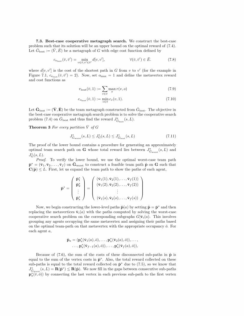
metavertex v, having occupancy o. We define the cost of an edge from v to v′ bypairing all final vertices of paths computed in v with all starting vertices of pathscomputed in v′, computing the costs of the shortest paths between them, and takingthe maximum of these costs. Figure 7.1 diagrams this process for two metavertices forwhich omax = 2. Suppose that the dotted lines represent optimal paths computed onboth metavertices for an occupancy of 1, and the dashed lines are the paths computedfor an occupancy of 2. The highlighted vertices represent the pair of ({final verticesin v}, {starting vertices in v′}) that are farthest apart. The cost of the shortest pathbetween these vertices is 7, hence ceworst
(v, v′) = 7 in this example. We can formally
21 1
7
G|v G|v’
Fig. 7.1. Example showing the worst-case edge-cost between two metavertices. Edge-costs are1 for edges within subgraphs, 2 for edges between subgraphs and all vertex costs are 0.
write the worst case metaedge cost function for all (v, v′) ∈ E, as
ceworst(v, v′) = max
o,o′
maxa,a′
d [p∗a(v, o, f), p∗a′(v′, o′, 1)] , (7.7)
where o, o′ ∈ O, a ∈ {1, . . . , o}, a ∈ {1, . . . , o′}, and d[v, v′] is the cost of the shortestpath in G from v to v′. In implementation, there are ways to make this less conser-vative. For example, one could create a team edge-cost function that depends on theoccupancies of adjacent vertices. However, for simplicity of notation, we choose anedge-cost on the location metagraph that does not depend on the vertex occupancies.
Now let Gworst := (V, E) be the team metagraph induced by Gworst. The teampath-cost and path-reward functions for the metagraph are defined exactly the sameas they were for the original graph in (7.2) and (7.3). The objective in the worst-casecooperative metagraph search problem is to solve the cooperative search problem (7.4)on Gworst and thus find the reward J∗
Gworst(s, L).
7.3. Best-case cooperative metagraph search. We construct the best-caseproblem such that its solution will be an upper bound on the optimal reward of (7.4).Let Gbest := (V , E) be a metagraph of G with edge cost function defined by
cebest(v, v′) = min
v∈v,v′∈v′
d[v, v′], ∀(v, v′) ∈ E. (7.8)
where d[v, v′] is the cost of the shortest path in G from v to v′ (for the example inFigure 7.1, cebest
(v, v′) = 2). Now, set omax = 1 and define the metavertex rewardand cost functions as
rbest(v, 1) :=∑
v∈v
maxo
r(v, o) (7.9)
cvbest(v, 1) := min
v∈vcv(v, 1). (7.10)
Let Gbest := (V, E) be the team metagraph constructed from Gbest. The objective inthe best-case cooperative metagraph search problem is to solve the cooperative searchproblem (7.4) on Gbest and thus find the reward J∗
Gbest(s, L).
Theorem 3 For every partition V of G
J∗Gworst
(s, L) ≤ J∗G(s, L) ≤ J∗
Gbest(s, L) (7.11)
The proof of the lower bound contains a procedure for generating an approximatelyoptimal team search path on G whose total reward lies between J∗
Gworst(s, L) and
J∗G(s, L).
Proof. To verify the lower bound, we use the optimal worst-case team pathp∗ = (v1, v2, . . . , vf ) on Gworst to construct a feasible team path p on G such thatC(p) ≤ L. First, let us expand the team path to show the paths of each agent,
p∗ =
p∗1
p∗2
...
p∗s
=
(v1(1), v2(1), . . . , vf (1))
(v1(2), v2(2), . . . , vf (2))...
(v1(s), v2(s), . . . , vf (s))
Now, we begin constructing the lower-level paths p(a) by setting p = p∗ and thenreplacing the metavertices vi(a) with the paths computed by solving the worst-casecooperative search problem on the corresponding subgraphs G|vi(a). This involvesgrouping any agents occupying the same metavertex and assigning their paths basedon the optimal team-path on that metavertex with the appropriate occupancy o. Foreach agent a,
pa = (p∗a(v1(a), o), . . . ,p∗
a(v2(a), o)), . . . ,
. . . ,p∗a(vf−1(a), o)), . . . ,p∗
a(vf (a), o)),
Because of (7.6), the sum of the costs of these disconnected sub-paths in p isequal to the sum of the vertex costs in p∗. Also, the total reward collected on thesesub-paths is equal to the total reward collected on p∗ due to (7.5), so we know thatJ∗
Gworst(s, L) = R(p∗) ≤ R(p). We now fill in the gaps between consecutive sub-paths
p∗a(v, o)) by connecting the last vertex in each previous sub-path to the first vertex
in the next sub-path with the shortest path in G between them. We know from(7.7) that the cost of these connections is less than or equal to the edge costs in p∗.Hence, C(p) ≤ C(p∗) ≤ L and p is a feasible path in G. Since p∗ is optimal on G,R(p) ≤ J∗
G(s, L), and the lower bound in 7.11 holds.To verify the upper bound, we construct a feasible path p in Gbest out of the
optimal search path p∗ = (v1,v2, . . . ,vf ) in G that generates reward R∗G(s, L). We
begin by setting p equal to p∗ and then replacing each vi(a) with the vi(a) thatcontains it. Now, we remove any consecutive repetitions from each pa, and then padthe end of agent’s paths with repeated metavertices where necessary to make thepaths of all agents the same length. This allows us to form the team-vertices thatmake up p, making a feasible path in Gbest without adding to the path-cost. We inferfrom (7.8) and (7.10) that C(p) ≤ C(p∗), so p meets the cost constraint. Finally,due to (7.9), all reward is collected from each metavertex visited by p, and the upperbound J∗
G(s, L) ≤ J∗Gbest
(s, L) holds.
7.4. Error Bounds for Simple Graphs. Although we can not expect to obtainconstant factor approximation bounds for arbitrary graphs, here we investigate theaccuracy of the fractal decomposition algorithm for the search problem on certainsimple graphs. Suppose a single agent is searching a rectangular lattice of size n =i2×i2, for i ∈ N, with a cost bound γn. The vertices all have zero cost and a reward ofone and all the edge costs are one. On this simple graph, the searcher can collect theoptimal reward of γn+1 in many ways, for example, by moving along the length of thefirst row and then proceeding row-by-row until the cost bound has been reached. Wenow apply the fractal decomposition algorithm by partitioning the graph evenly into√
n square subgraphs each containing√
n metavertices and choosing a meta-vertexcost bound of
√n. The lower bound on the optimal search reward, determined by the
reward collected on the worst-case meta-graph, is
√n
⌊
γn√
n + 3n14 − 3
⌋
,
where the term√
n on the left indicates the reward colected in each meta-vertex, andthe term on the right is the conservative worst-case estimate of the number of meta-vertices the searcher can visit. The resulting ratio of worst-case reward to optimalreward is
√n⌊
γn√
n+3n14 −3
⌋
γn − 1.
Notice that as n gets large, the ratio approaches one. This is because the cost incurredin searching a meta-vertex grows as n2 while the cost incurred in transit betweenmeta-vertices only grows as fast as n. This result extends recursively for multiple de-compostion levels. We conclude that for large graphs, where the transit cost betweenmetavertices is small compared to the cost of searching a metavertex, the lower-boundon the search reward may be very close to optimal.
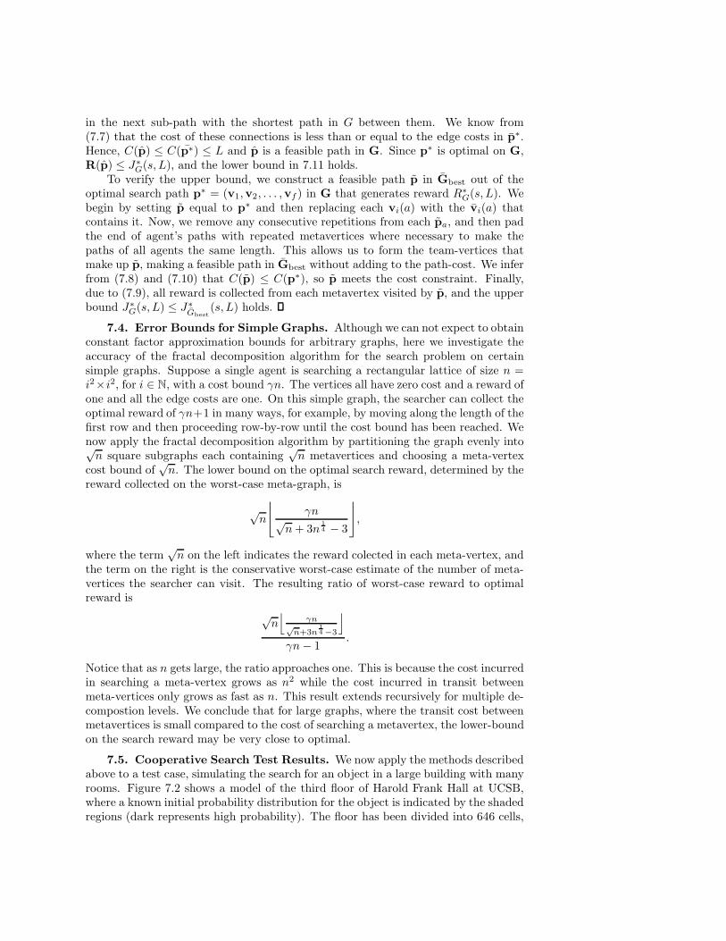
7.5. Cooperative Search Test Results. We now apply the methods describedabove to a test case, simulating the search for an object in a large building with manyrooms. Figure 7.2 shows a model of the third floor of Harold Frank Hall at UCSB,where a known initial probability distribution for the object is indicated by the shadedregions (dark represents high probability). The floor has been divided into 646 cells,
each about 4 square meters in size. There is a graph vertex on each cell and pairs ofvertices lying on adjacent cells are connected by an edge in the graph. We assign eachedge a cost of 1, modeling a one second transit time between cells, and each vertex acost of 2, supposing that it takes 2 seconds to search a cell.
Fig. 7.2. Model of third floor of UCSB’s Harold Frank Hall divided into 646 cells and overlaidwith a graph. Dark cells indicate high target probability.
In this test case, we have 4 searchers and only two minutes to find the object. Thegoal is to find the path for each agent that approximately maximizes the probabilityof finding the object in 120 seconds. To get an idea of the magnitude of computationposed by this problem, consider a solution by total enumeration of feasible paths. Theaverage degree of a vertex in this graph is about 3, meaning that the average degreeof a vertex in the team graph is 34 = 81, that is, there are about 81 possible movesfor the team at each vertex. A cost bound of 120 allows the searchers to visit up to40 vertices along their paths. This translates to roughly 8140 ≈ 1076 paths that mustbe evaluated to find the optimal search path by total enumeration.
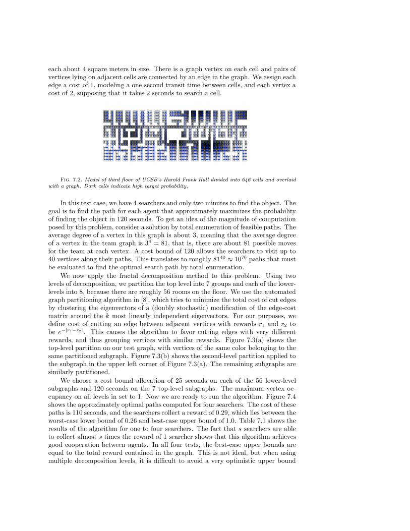
We now apply the fractal decomposition method to this problem. Using twolevels of decomposition, we partition the top level into 7 groups and each of the lower-levels into 8, because there are roughly 56 rooms on the floor. We use the automatedgraph partitioning algorithm in [8], which tries to minimize the total cost of cut edgesby clustering the eigenvectors of a (doubly stochastic) modification of the edge-costmatrix around the k most linearly independent eigenvectors. For our purposes, wedefine cost of cutting an edge between adjacent vertices with rewards r1 and r2 tobe e−|r1−r2|. This causes the algorithm to favor cutting edges with very differentrewards, and thus grouping vertices with similar rewards. Figure 7.3(a) shows thetop-level partition on our test graph, with vertices of the same color belonging to thesame partitioned subgraph. Figure 7.3(b) shows the second-level partition applied tothe subgraph in the upper left corner of Figure 7.3(a). The remaining subgraphs aresimilarly partitioned.
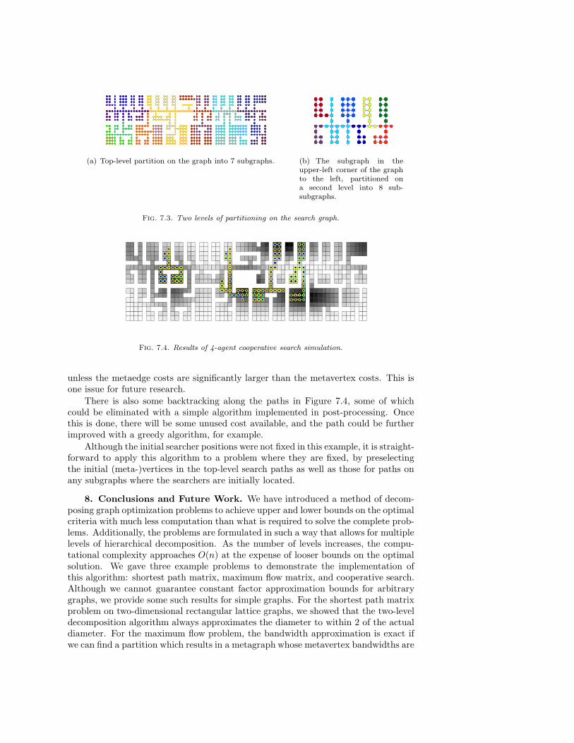
We choose a cost bound allocation of 25 seconds on each of the 56 lower-levelsubgraphs and 120 seconds on the 7 top-level subgraphs. The maximum vertex oc-cupancy on all levels in set to 1. Now we are ready to run the algorithm. Figure 7.4shows the approximately optimal paths computed for four searchers. The cost of thesepaths is 110 seconds, and the searchers collect a reward of 0.29, which lies between theworst-case lower bound of 0.26 and best-case upper bound of 1.0. Table 7.1 shows theresults of the algorithm for one to four searchers. The fact that s searchers are ableto collect almost s times the reward of 1 searcher shows that this algorithm achievesgood cooperation between agents. In all four tests, the best-case upper bounds areequal to the total reward contained in the graph. This is not ideal, but when usingmultiple decomposition levels, it is difficult to avoid a very optimistic upper bound
(a) Top-level partition on the graph into 7 subgraphs. (b) The subgraph in theupper-left corner of the graphto the left, partitioned ona second level into 8 sub-subgraphs.
Fig. 7.3. Two levels of partitioning on the search graph.
Fig. 7.4. Results of 4-agent cooperative search simulation.
unless the metaedge costs are significantly larger than the metavertex costs. This isone issue for future research.
There is also some backtracking along the paths in Figure 7.4, some of whichcould be eliminated with a simple algorithm implemented in post-processing. Oncethis is done, there will be some unused cost available, and the path could be furtherimproved with a greedy algorithm, for example.
Although the initial searcher positions were not fixed in this example, it is straight-forward to apply this algorithm to a problem where they are fixed, by preselectingthe initial (meta-)vertices in the top-level search paths as well as those for paths onany subgraphs where the searchers are initially located.
8. Conclusions and Future Work. We have introduced a method of decom-posing graph optimization problems to achieve upper and lower bounds on the optimalcriteria with much less computation than what is required to solve the complete prob-lems. Additionally, the problems are formulated in such a way that allows for multiplelevels of hierarchical decomposition. As the number of levels increases, the compu-tational complexity approaches O(n) at the expense of looser bounds on the optimalsolution. We gave three example problems to demonstrate the implementation ofthis algorithm: shortest path matrix, maximum flow matrix, and cooperative search.Although we cannot guarantee constant factor approximation bounds for arbitrarygraphs, we provide some such results for simple graphs. For the shortest path matrixproblem on two-dimensional rectangular lattice graphs, we showed that the two-leveldecomposition algorithm always approximates the diameter to within 2 of the actualdiameter. For the maximum flow problem, the bandwidth approximation is exact ifwe can find a partition which results in a metagraph whose metavertex bandwidths are
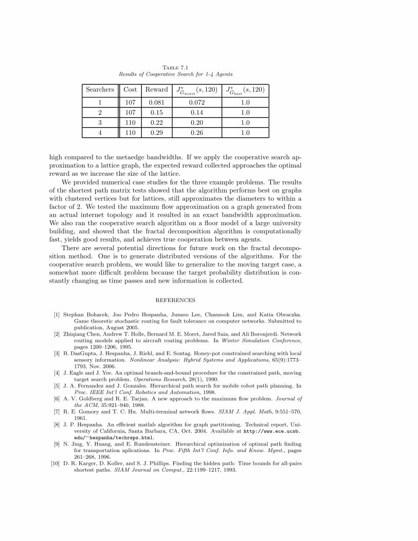
Table 7.1
Results of Cooperative Search for 1-4 Agents
Searchers Cost Reward J∗Gworst
(s, 120) J∗Gbest
(s, 120)
1 107 0.081 0.072 1.0
2 107 0.15 0.14 1.0
3 110 0.22 0.20 1.0
4 110 0.29 0.26 1.0
high compared to the metaedge bandwidths. If we apply the cooperative search ap-proximation to a lattice graph, the expected reward collected approaches the optimalreward as we increase the size of the lattice.
We provided numerical case studies for the three example problems. The resultsof the shortest path matrix tests showed that the algorithm performs best on graphswith clustered vertices but for lattices, still approximates the diameters to within afactor of 2. We tested the maximum flow approximation on a graph generated froman actual internet topology and it resulted in an exact bandwidth approximation.We also ran the cooperative search algorithm on a floor model of a large universitybuilding, and showed that the fractal decomposition algorithm is computationallyfast, yields good results, and achieves true cooperation between agents.
There are several potential directions for future work on the fractal decompo-sition method. One is to generate distributed versions of the algorithms. For thecooperative search problem, we would like to generalize to the moving target case, asomewhat more difficult problem because the target probability distribution is con-stantly changing as time passes and new information is collected.
REFERENCES
[1] Stephan Bohacek, Joo Pedro Hespanha, Junsoo Lee, Chansook Lim, and Katia Obraczka.Game theoretic stochastic routing for fault tolerance on computer networks. Submitted topublication, August 2005.
[2] Zhiqiang Chen, Andrew T. Holle, Bernard M. E. Moret, Jared Saia, and Ali Boroujerdi. Networkrouting models applied to aircraft routing problems. In Winter Simulation Conference,pages 1200–1206, 1995.
[3] B. DasGupta, J. Hespanha, J. Riehl, and E. Sontag. Honey-pot constrained searching with localsensory information. Nonlinear Analysis: Hybrid Systems and Applications, 65(9):1773–1793, Nov. 2006.
[4] J. Eagle and J. Yee. An optimal branch-and-bound procedure for the constrained path, movingtarget search problem. Operations Research, 28(1), 1990.
[5] J. A. Fernandez and J. Gonzales. Hierarchical path search for mobile robot path planning. InProc. IEEE Int’l Conf. Robotics and Automation, 1998.
[6] A. V. Goldberg and R. E. Tarjan. A new approach to the maximum flow problem. Journal ofthe ACM, 35:921–940, 1988.
[7] R. E. Gomory and T. C. Hu. Multi-terminal network flows. SIAM J. Appl. Math, 9:551–570,1961.
[8] J. P. Hespanha. An efficient matlab algorithm for graph partitioning. Technical report, Uni-versity of California, Santa Barbara, CA, Oct. 2004. Available at http://www.ece.ucsb.
edu/∼hespanha/techreps.html.[9] N. Jing, Y. Huang, and E. Rundensteiner. Hierarchical optimization of optimal path finding
for transportation aplications. In Proc. Fifth Int’l Conf. Info. and Know. Mgmt., pages261–268, 1996.
[10] D. R. Karger, D. Koller, and S. J. Phillips. Finding the hidden path: Time bounds for all-pairsshortest paths. SIAM Journal on Comput., 22:1199–1217, 1993.
[11] J. Kim and J. Hespanha. Discrete approximations to continuous shortest-path: Application tominimum-risk path planning for groups of UAVs. In Proc. of the 42nd IEEE Conferenceon Decision and Control, 2003.
[12] C. Lim, S. Bohacek, J. Hespanham, and K. Obraczka. Hierarchical max-flow routing. In Proc.of the IEEE GLOBECOM, 2005.
[13] J. R. Riehl and J. P. Hespanha. Fractal graph optimization algorithms. In Proceedings of the44th Conference on Decision and Control, 2005.
[14] H. E. Romeijn and R. L. Smith. Parallel algorithms for solving aggregated shortest pathproblems. Computers and Operations Research, 26:941–953, 1999.
[15] G. Shen and P. E. Caines. Hierarchically accelerated dynamic programming for finite-statemachines. IEEE Transactions on Automatic Control, 47(2):271–283, 2002.
[16] N. Spring, R. Mahajan, D. Wetherall, and T. Anderson. Measuring isp topologies with rocket-fuel. Transactions on Networking, 12, 2004.
[17] K. E. Trummel and J.R. Weisinger. The complexity of the optimal searcher path problem.Operations Research, 34(2):324–327, 1986.