graph theory notes of new york lviigtn.kazlow.info/gtn57.pdfgraph theory notes of new york lvii...
TRANSCRIPT
GRAPH THEORY NOTESOF NEW YORK
Editors:John W. KennedyLouis V. Quintas
The Metropolitan New York Section of
LVII
(2009)
Dedicated to the memory of
Gary S. Bloom

Graph Theory Notes of New York
Graph Theory Notes of New York
publishes short contributions andresearch articles in graph theory, its related fields, and its applications.
Founding Editors: John W. Kennedy (Queens College, CUNY)
Louis V. Quintas (Pace University)
Editorial Address: Graph Theory Notes of New York
Mathematics Department
Queens College, CUNY
Kissina Boulevard
Flushing, NY 11367, U.S.A.
Editorial Board: Brian R. Alspach (University of Newcastle, AUSTRALIA)
Krystyna T. Bali
ƒ
ska (Technical University of Pozna
ƒ
, POLAND)
Peter R. Christopher (Worcester Polytechnic Institute, Massachusetts)
Edward J. Farrell (University of the West Indies, TRINIDAD)
Ralucca M. Gera (Naval Postgraduate School, California)
Ivan Gutman (University of Kragujevac,YUGOSLAVIA)
Michael Kazlow (Pace University, New York)
Linda Lesniak (Drew University, New Jersey)
Irene Sciriha (University of Malta, MALTA)
Peter J. Slater (University of Alabama at Huntsville, Alabama)
Richard Steinberg (London School of Economics, ENGLAND, U.K.)
Christina M.D. Zamfirescu (Hunter College, CUNY, New York)
Published by: The Metropolitan New York Section of the
Mathematical Association of America
<http://www.maa.org/metrony>
Composit:
K-M Research
50 Sudbury Lane
Westbury, NY 11590, U.S.A.
ISSN 1040-8118
Information for contributors can be found on the inside back cover.

Metropolitan New York Section
GRAPH THEORY NOTES
OF NEW YORK
LVII
(2009)
This issue includes papers presented at
Graph Theory Day 57
held at
The Department of Mathematics, Computer Science, and Information Technology
Nassau Community College, SUNY
Garden City, New York
Saturday, May 16, 2009
Dedicated to the memory of
Gary S. Bloom

Graph Theory Notes of New York LVII The Mathematical Association of America (2009)
CONTENTS
Introductory Remarks [GTN LVII: 5
Graph Theory Day 57 6
:1] Oblong graphs; A. Delgado 10
:2] The nature of graph theory: A visitor kibitzes; W. Meyer 14
:3] The travelling salesperson problem: Let us plan a road trip! I. Klikovac 24
:4] Some questions on graph protection; W.F. Klostermeyer 29
:5] On two conjectures about faulty hypercubes; N. Castañeda, V.S. Gochev, I. Gotchev, and F. Latour 34
:6] An inequality for the signless Laplacian index of a graph using the chromatic number; P. Hansen and C. Lucas 39
:7] The integral sum graph; K. Vilfred and T. Nicholas 43
[GTN LVII] Key-Word Index 48

Graph Theory Notes of New York LVII (2009) 5
INTRODUCTORY REMARKS
This issue of
Graph Theory Notes of New York
is dedicated to Gary S. Bloom (1940–2009). Gary died onSeptember 6, 2009 while hiking in Great Barrington, Massachusetts. He was born in Los Angeles, attendedhigh school in Bexley, Ohio, earned an A.B. in Physics from Oberlin College, Ohio, an M.S. in Astrophysicsfrom the University of Arizona, and in 1976 a Ph.D. in Electrical Engineering from The University of South-ern California. With these widespread interests it is not surprising that his ultimate research activities cen-tered on diverse applications of graph theory. His personal interests were also varied, including, tangodancing, hiking, theater, music, and art, especially art of the Southwest. Always looking at the humorousside of life he enjoyed sharing both good and bad puns. One of his favorite openings lines for seminar andconference talks was to note that a an anagram of G.S. Bloom is S. Golomb (Solomon Golomb was Gary'sPh.D. advisor).
Gary’s teaching career started in 1969 at California State College, Fullerton and then, in 1976, he joined thefaculties of Computer Science at The City College of New York and the Graduate Center of The City Uni-versity of New York. He maintained these as his permanent positions while undertaking visiting teachingand research positions in Australia, Canada, Chile, France, and Spain.
We especially remember Gary as a good friend, always enjoyable to be with, and a creative research col-league. Gary was very involved in the beginnings of Graph Theory Days and
Graph Theory Notes
. He wason the organizing committee of the first Graph Theory Day in 1981 and was a consistent participant andcontributor to many of the Graph Theory Days that followed. His articles in
Graph Theory Notes of NewYork
are among his many publications. His support of the development of the
Notes
is greatly appreciated.
We shall carry on with very good memories of Gary.
JWK/LVQNew York
December 2009

6 Graph Theory Notes of New York LVII (2009)
GRAPH THEORY DAY 57
Organizing Committee
Graph Theory day 57, was sponsored by The Metropolitan New York Section of The Mathematical Associ-ation of America and was hosted by the Department of Mathematics, Computer Science, and InformationTechnology at Nassau Community College, SUNY, Garden City, New York on Saturday May 16, 2009. JayMartin (NCC) opened the event and introduced Sean Fanelli, President of NCC who made the welcomingremarks. Carmine DeSanto, Chair of the hosting department at NCC provided a few more words of welcomeand joined Jay in introducing the featured speakers.
The featured presentations at Graph Theory Day 57 were:
The Nature of Graph Theory: A Visitor Kibitzes
Walter Meyer [See this issue page 14]Department of MathematicsAdelphi UniversityGarden City, New York, U.S.A.
Generalized Dice Games and Their Associated Graphs
Lorenzo Traldi [See issue LIII page 39]Department of MathematicsLafayette CollegeEaston, Pennsylvania, U.S.A.
Participants at Graph Theory Day 57
Alexander Atwood Mathematics DepartmentSuffolk County Community College533 College Road, Selden, NY [email protected]
Chris Atwood Department of Eng/Phys/TechNassau Community CollegeOne Education Drive, Garden City, NY [email protected]
Armen R. Baderian Department of MAT/CSC/ITENassau Community CollegeGarden City, NY [email protected]
Jack-Kang Chan Department of Mathematics and Computer ScienceQueensborough Community College153-16, 58th Avenue, Flushing, NY [email protected]
Robert Cowen Department of MathematicsQueens College, CUNY164-22 75 Avenue, Flushing, NY [email protected]
Anthony Delgado Department of Natural SciencesPurchase College, SUNY82-06 60th Road, Middle Village, NY [email protected]
Co-Chairs: Mohammed Javadi, Lilia Orlova, and Ronald Skurnick(Nassau Community College, SUNY)
Armen Baderian and Jay Martin (Nassau Community College, SUNY)
John W. Kennedy (Queens College, CUNY), Louis V. Quintas (Pace University)

Graph Theory Notes of New York LVII (2009) 7
Carmine DeSanto Department of MAT/CSC/ITENassau Community College, SUNYOne Education Drive, Garden City, NY [email protected]
Kimberly Dwyer Mathematics DepartmentSyosset High School29 Libby Avenue, Hicksville, NY [email protected]
Sean Fanelli PresidentNassau Community College, SUNYOne Education Drive, Garden City, NY [email protected]
Joseph Edward Fields Department of MathematicsSouthern Connecticut State University501 Crescent Street, New Haven, CT [email protected]
Christopher Hanusa Mathematics DepartmentQueens College6530 Kissena Boulevard, Flushing, NY [email protected]
Stephen H. Hechler Department of MathematicsQueens College, CUNY9 Greendale Lane, East Northport, NY [email protected]
David Herscovici Department of Computer Science and Digital DesignQuinnipiac University275 Mount Carmel Avenue, CL-AC1, Hamden, CT [email protected]
Heather Huntington Department of MAT/CSC/ITENassau Community CollegeOne Education Drive, Garden City, NY [email protected]
Mohammad Javadi Department of MAT/CSC/ITENassau Community College, SUNYOne Education Drive, Garden City, NY [email protected]
Art Kalish Mathematics DepartmentSyosset High School6 Rochester Court, Huntington, NY [email protected]
John W. Kennedy Department of MathematicsQueens College, CUNY50 Sudbury Lane, Westbury, NY [email protected]
Myungchul Kim Mathematics DepartmentSuffolk County Community College533 College Road, Selden, NY [email protected]
Ida Klikovac Department of MAT/CSC/ITENassau Community College, SUNYOne Education Drive, Garden City, NY [email protected]
Frederic Latour Department of Mathematical SciencesCentral Connecticut State University1615 Stanley Street, New Britain, CT [email protected]

8 Graph Theory Notes of New York LVII (2009)
Kenneth Lemp Department of MAT/CSC/ITENassau Community College, SUNYOne Education Drive, Garden City, NY [email protected]
Marty Lewinter Division of Natural SciencesPurchase College, SUNY735 Anderson Hill Road, Purchase, NY [email protected]
Lorraine L. Lurie Mathematics DepartmentPace University370 Ocean Parkway, 10C, Brooklyn, NY [email protected]
Joseph Malkevitch Department of MathematicsYork College, CUNY6 Garden City Street, Garden City, NY [email protected]
Dennis Manderino Pace University2151 East 12th Street, Brooklyn, NY [email protected]
Jay Martin Department MAT/CSC/ITENassau Community College, SUNYOne Education Drive, Garden City, NY [email protected]
Rochelle Meyer Department of MAT/CSC/ISENassau Community College, SUNY100 Brook Street, Garden City, NY [email protected]
Walter Meyer Department of MathematicsAdelphi UniversityGarden City, NY [email protected]
Calvin H. Mittman Department of Mathematics and Computer ScienceSt. John's UniversitySt. John Hall, Room 334, Jamaica, NY [email protected]
Lilia Orlova Department of MAT/CSC/ITENassau Community College, SUNYOne Education Drive, Garden City, NY [email protected]
Cheng Qian Department of MathematicsNassau Community College, SUNY35-40 Taft Street, Wantagh, NY [email protected]
Louis V. Quintas Department of MathematicsPace UniversityOne Pace Plaza, New York, NY [email protected]
Sylvester Reese Mathematics and CS DepartmentQueenborough Community CollegeP.O. Box 131, New York, NY [email protected]
Brian Richter SW EngineeringTelephonics [email protected]

Graph Theory Notes of New York LVII (2009) 9
Gabriel Rosenberg Mathematics DepartmentPace University1191 Sylvia Road, Seaford, NY [email protected]
Judie Schwartz Department of MathematicsNassau Community College, SUNYOne Education Drive, Garden City, NY [email protected]
Ronald Skurnick Department of MAT/CSC/ITENassau Community CollegeOne Education Drive, Garden City, NY [email protected]
JoAnne Taormina Department of MAT/CSC/ITENassau Community College, SUNYOne Education Drive, Garden City, NY [email protected]
Lorenzo Traldi Department of MathematicsLafayette CollegeEaston, PA [email protected]
Walter Vohs Mathematics DepartmentNassau Community College, SUNYOne Education Drive, Garden City, NY [email protected]
Jack Winn Department of MathematicsFarmingdale State College, SUNYFarmingdale, NY [email protected]

Graph Theory Notes of New York LVII, 10–13 (2009)The Mathematical Association of America.
[GTN LVII:1] OBLONG GRAPHS
Anthony Delgado
Division of Natural SciencePurchase CollegePurchase, New York 10577, U.S.A.<[email protected]>
1. Introduction
An integer is called
oblong
if it can be written in the form for some integer ,
[1]
. Denote the
n
th
oblong number, , by
O
n
. A graph
G
is an
oblong graph
if
1. The vertices of
G
are labeled by distinct oblong numbers.
2. Each edge of
G
is labeled by the product of the labels of its end vertices.
3. The edge labels are distinct oblong numbers.
(A given vertex and a given edge can share the same oblong label.)
The path graph
P
4
of order 4 is oblong, as can be seen by labeling the vertices by 2, 6, 12, and 20 in that order.The edge labels are then 12, 72, and 240, all of which are oblong integers. The star graph is oblong.Label the center vertex 2, and label the three end-vertices 6, 210, and . The edge labelsare then 12, 420, and . Finally, the cycle graph
C
14
is oblong, as can be seen by labelingthe vertices consecutively 2, 6, 12, 20, 30, 42, 56, 72, 90, 110, 132, 156, 182, and 210. The edge labels are dis-tinct, and they increase monotonically with the exception of the last edge label, 420. However, this last labelis also distinct since the first few edge labels are 12, 72, 240, and 600.
The first theorem states that the product of two consecutive oblong numbers, with indices
n
and is theoblong number with index .
Theorem 1:
For each positive integer
n
, , where .
Proof:
By definition, . Thus,
where .
�
Corollary 1:
The path , of order
n
, is oblong for each .
�
2. Main Results
We now seek pairs of nonconsecutive oblong numbers and , such that the pairwise product isoblong.
Let
λ
be a fixed oblong number. We seek infinitely many pairs of positive integers
n
and
t
, such that; that is,
or ,
which yields the quadratic equation
.
The solution to this quadratic is given by
(1)
,
n n 1+( ) n 1≥n n 1+( )
K1 3,242556 492 493( )=
485112 696 697( )=
n 1+n2 2n+
OnOn 1+ Om= m n2 2n+=
On n n 1+( )=
OnOn 1+ n n 1+( ) n 1+( ) n 2+( )=
n n 2+( )[ ] n 1+( )2=
n2 2n+( ) n2 2n 1+ +( ) Om= =
m n2 2n+=
Pn n 1≥
Ox Oy OxOy
λOn On t+=
λn n 1+( ) n t+( ) n t 1+ +( )= λn2 λn+ n2 2nt t2 n t+ + + +=
λ 1–( )n2 λ 1– 2t–( )n t t 1+( )–+ 0=
n 2t λ– 1 D+ +2 λ 1–( )
--------------------------------------=

A. Delgado: Oblong graphs 11
where the discriminant .
Let to obtain
(2) .
Since D in (1) must be a square, let . A little algebra then yields
(3) .
Now consider the Pell equation (see (1A) in the Appendix),
(4) .
Note that oblong numbers are not squares, thus λ is not a square. Hence (4) has infinitely many solutions. Thesubstitutions
and
yield solutions to (3), as can be seen by substituting them into (3). We obtain
.
On canceling , this becomes (4). We now show that y is even, thereby justifying .
Let , then an initial solution to (4) is and , as can be seen by inserting thesevalues for x and y, to obtain
.
Consulting the Appendix, we see that
.
Now
and
.
Subtracting the second from the first, we obtain
.
Dividing by yields
.
Because appears in every term, y is even for all m. On the other hand, by (4), x is always odd.
Rewriting (1) with several substitutions (including ) yields
(5) ,
which is a (positive) integer since x and y have opposite parity.
We have now proved the following theorem:
Theorem 2: Given the oblong number λ, the equation has infinitely many solutions. �
D λ 1– 2t–( )2 4 λ 1–( )t t 1+( )+=
λ λ 1–=
D λ 2t–( )2 4λt t 1+( )+=
D s2=
s2 4λt2– λ2=
x2 λy2– 1=
s λx= 2t λy=
λx( )2 λ λy( )2– λ2=
λ2 2t λy=
λ j j 1+( )= a 2 j 1+= b 2=
2 j 1+( )2 4 j j 1+( )– 4 j2 4 j 1 4 j2– 4 j–+ + 1= =
y a λb+( )m a λb–( )m–
2 λ---------------------------------------------------------------=
a λb+( )m am m1⎝ ⎠
⎛ ⎞ λ1 2/ am 1– b m2⎝ ⎠
⎛ ⎞ λam 2– b2 m3⎝ ⎠
⎛ ⎞ λ3 2/ am 3– b3 m4⎝ ⎠
⎛ ⎞ λ2am 4– b4 …+ + + + +=
a λb–( )m am m1⎝ ⎠
⎛ ⎞ λ1 2/ am 1– b– m2⎝ ⎠
⎛ ⎞ λam 2– b2 m3⎝ ⎠
⎛ ⎞ λ3 2/ am 3– b3– m4⎝ ⎠
⎛ ⎞ λ2am 4– b4 …–+ +=
a λb+( )m a λb–( )m– 2 m1⎝ ⎠
⎛ ⎞ λ1 2/ am 1– b m3⎝ ⎠
⎛ ⎞ λ3 2/ am 3– b3 m5⎝ ⎠
⎛ ⎞ λ5 2/ am 5– b5 …+ + +=
2λ1 2/
y m1⎝ ⎠
⎛ ⎞ am 1– b m3⎝ ⎠
⎛ ⎞ λam 3– b3 m5⎝ ⎠
⎛ ⎞ λ2am 5– b5 …+ + +=
b 2=
D s2=
n 2t λ– 1 s+ +2 λ 1–( )
-------------------------------- yλ λ– xλ+
2λ---------------------------- y 1– x+
2---------------------= = =
λOn On 1+=

12 Graph Theory Notes of New York LVII (2009)
Now let (so that ) to obtain solutions for , for which an initial solution is and (see the Appendix). Then and . By (5),
and . This yields the solution , or , in which the oblong numbers onthe left are consecutive. To obtain this consecutive solution and infinitely many nonconsecutive solutions (for
), we employ the method detailed in the Appendix. (The consecutive solution is obtained using.)
(6)
By letting , for example, we obtain and . Then from (5) and (6) we obtain .
Observing that , we obtain .
The next theorem yields an infinite class of oblong cycle graphs. We require the following definition andlemma.
Definition: A number is 2-long if it is of the form . �
Remark: The oblong number in Theorem 1 is the nth 2-long number.
Lemma 1: A number is 2-long if and only if it is one less than a square.
Proof: Follows at once from the fact that . �
The proof of the next theorem uses the following observation:
Remark: Using the binomial expansion with and the equations in (6) can be written as
(7)
Theorem 3: The cycle graph is oblong, where ,and and are as defined in (6).
Proof: Label the n vertices of using distinct oblong numbers starting with 2. By Theorem 1, the first edges will be labeled with consecutive oblong numbers. By Theorem 2, the label of the last edge will
be . By (5), . Since , then . Toshow that the label of the last edge is distinct from each of the other edge labels, we show that its index, ,is not 2-long and apply Theorem 1. By Lemma 1, this is equivalent to showing that is not a square,or is not a square. From (7), we obtain
,
in which case, (mod 3). Since (mod 3), it follows that (mod 3), from which it follows that it is not a square, thereby proving the theorem.
�
The following definition is found in [3].
Definition: Given a nonnegative integer k, an integer m is k-long if for some integer . �
Note that when , we obtain the oblong numbers. In [2] k-long graphs are defined in a manner that gen-eralizes oblong graphs. Many new results are derived and various open problems are presented.
Acknowledgements
The author thanks Professors Marty Lewinter, Purchase College, and Lou Quintas, Pace University, for theirgenerous assistance.
λ 2= λ 1= x2 2y2– 1=x a 3= = y b 2= = s 3= t 1= n 2 1– 3+( ) 2⁄ 2= =
n t+ 3= 2O2 O3= 2 2 3×[ ] 3 4×=
λ 2=m 1=
xm3 2 2+( )m 3 2 2–( )m+
2--------------------------------------------------------------- s= =
ym3 2 2+( )m 3 2 2–( )m–
2 2-------------------------------------------------------------- 2t= =
m 2= x2 17= y2 12= n 14=
t y 2⁄ 6= = 2O14 O20=
n n 2+( )On2 2n+
n n 2+( ) n 1+( )2 1–=
a 3= b 2 2=
xm 3m m2⎝ ⎠
⎛ ⎞ 233m 2– m4⎝ ⎠
⎛ ⎞ 263m 4– m6⎝ ⎠
⎛ ⎞ 293m 6– …+ + + +=
ymm1⎝ ⎠
⎛ ⎞ 213m 1– m3⎝ ⎠
⎛ ⎞ 243m 3– m5⎝ ⎠
⎛ ⎞ 273m 5– …+ + +=
Cn n ym 1– xm+( ) 2⁄=xm ym
Cnn 1–
2On1 On t+
1= n ym 1– xm+( ) 2⁄= t ym 2⁄= n t+ 2ym 1– xm+( ) 2⁄=n t+
n t 1+ +2ym 1 xm+ +( ) 2⁄
2ym 1 xm+ +
2-------------------------------- 3m 1+
2---------------- m
1⎝ ⎠⎛ ⎞ 213m 1– m
2⎝ ⎠⎛ ⎞ 223m 2– m
3⎝ ⎠⎛ ⎞ 243m 3– m
4⎝ ⎠⎛ ⎞ 253m 4– m
5⎝ ⎠⎛ ⎞ 273m 5– …+ + + + + +=
2ym 1 xm+ +( ) 2⁄ 3m 1+( ) 2⁄= 3m 1+ 4=3m 1+( ) 2⁄ 2=
m n n k+( )= n 1≥k 1=

A. Delgado: Oblong graphs 13
References
[1] D.M. Burton; Elementary Number Theory, 4th ed., McGraw-Hill (1998).
[2] A. Delgado, M. Gargano, M. Lewinter, and J. Malerba; Introducing k-long numbers, Cong. Num., 189, 15–23 (2008).
[3] A. Delgado, M. Lewinter, and L.V. Quintas; k-long graphs, Cong. Num. (2009) — accepted.
Appendix
An equation of the form
(1A) ,
where and k is not a square, and x and y are positive integers is called a Pell equation. If k is a square,say , (1A) becomes , which has no positive integer solution.
Here is a method for obtaining infinitely many solutions to (1A). The first step is to find a pair of positive inte-gers a and b that satisfy the equation; that is, a and b satisfy . Now suppose that x and y also sat-isfy (1A). Then for any ,
(2A ,
since . The next step is to factor both and as the difference of two squares,even though k might not be a square. Then (2A) becomes
,
which we transform into
To solve for x, add these equations and divide by 2. To solve for y, subtract and divide by . We obtaininfinitely many solutions:
These equations yield positive integers despite the presence of .
Received: July 10, 2008
x2 ky2– 1=
k 2≥k c2= x2 cy( )2– 1=
a2 kb2– 1=m 2 3 4 …, , ,=
x2 ky2– a2 kb2–( )m=
a2 kb2– 1= x2 ky2– a2 kb2–
x ky–( ) x ky+( ) a kb–( )m a kb+( )m=
x ky+ a kb+( )m=
x ky– a kb–( )m=
2 k
x a kb+( )m a kb–( )m+2
--------------------------------------------------------------=
y a kb+( )m a kb–( )m–2
--------------------------------------------------------------=
k

Graph Theory Notes of New York LVII, 14–23 (2009)The Mathematical Association of America.
[GTN LVII:2] THE NATURE OF GRAPH THEORY: A VISITOR KIBITZES
Walter MeyerDepartment of MathematicsAdelphi UniversityGarden City, New York 11791, U.S.A.<[email protected]>
1. Introduction
My title is meant as an exercise in modesty. I call myself a visitor because, although I have done work in graphtheory, I am not primarily a graph theorist—many readers have better credentials in this field than I do. How-ever, my hope is that even a visitor might have interesting perspectives on the big picture of this subject. Call-ing myself a kibitzer1 is meant to signify that I have in mind something much more informal that an exercisein the philosophy of knowledge or in the foundations of mathematics. What I have in mind is to reflect onthree rather different times in my professional life when I have worked in graph theory: First, when it cameup in a pure mathematics investigation; second, when it came up in applied work I did while working in indus-try; last, when my wife, Rochelle Meyer, and I were writing material for a book for general education coursesin mathematics [1].
2. Sylvester’s Problem and Its Dual
In 1893, J.J. Sylvester [2] asked the following question:
If n points in the plane are not colinear, must it be true that at least one linedetermined by pairs of these points has only two of the given points on it?
In this context, a line with only two of the points on it is called an ordinary line. In 1940 it was establishedthat there must be at least one ordinary line. By the time I got interested, in the early 1970s, the best resultasserted that there were always at least ordinary lines [3]. For example, see Figure 1.
1 This recent addition to English come to us from Yiddish where it means an onlooker giving sometimes unsolicited ad-vice—for example, someone watching a chess match. It arrives in Yiddish from the German word kiebitz meaning thebird known in English as the peewit, green plover, or lapwing. I hope to do a bit better in this article than the chatteringof a bird.
3n 7⁄
Figure 1: Sylvester’s problem (the original).

W. Meyer: The nature of graph theory: A visitor kibitzes 15
A dual version of Sylvester’s problem can also be posed:
Given n lines, not all concurrent or parallel, how many ordinary points must there be?
An ordinary point is a point at which just two of the given lines cross.
Again, at the time of my interest in these matters, it was known that there must be ordinary lines (seeFigure 2). However, here is the remarkable part. The lines can be replaced by wiggly versions, called pseudo-lines, and give the same result (see Figure 3). Technically a pseudoline is the image of a line under ahomeomorphism of the plane onto itself. Alternatively, from an inverse point of view, there is a homeomor-phism that turns the pseudoline to a line.
To appreciate the fact that the same result is obtained for both pseudolines and lines, one needs to understandthat in an arrangement of pseudolines, each pseudoline results from its own homeomorphism. Examples showthat there may be no single homeomorphism that simultaneously turns all the pseudolines back to lines. (Ifthere were such a homeomorphism, the result about ordinary points for lines would immediately give thesame result for any arrangement of pseudolines.) A nice discussion of an example where it is impossible tosimultaneously stretch all pseudolines back to straight lines can be found at:
<http://www.ams.org/featurecolumn/archive/oriented4.html>
For more extensive material along these lines see Grünmaum [4] and Ringel [5][6].
This circle of ideas seems to me to be remarkable in that Sylvester’s problem and its dual version seem to beessentially about straightness. If someone had told me that you could prove things about arrangements of lineswith just the axioms of projective geometry, I might have believed that. However, that it came down to topol-ogy, or, as we could also say, planar graph theory, seemed to put Euclid’s geometry into a new light.
In view of these matters about lines and pseudolines, I began to investigate simple closed curves in the planeand their intersection patterns. In an arrangement of curves we assume that we have n simple closed curves
Figure 2: Sylvester’s problem (dual version) n = 6, six ordinary points.
3n 7⁄
3n 7⁄
Figure 3: An arrangement of pseudolines.

16 Graph Theory Notes of New York LVII (2009)
where each pair intersect twice. We also assume that none of the regions in the complement of the set ofcurves is two-sided. Under these circumstances, I was able to prove that there must be at least ordinarypoints—points where just two curves cross. Figure 4 illustrates an example with having 8 ordinarypoints. To my knowledge, this has not been pursued much since and it may still be the best result known.However, I doubt that it is a best possible bound. There is probably a lot to be discovered here.
3. Robotics and Visibility Graphs
Some years later, in the late 1980s and 1990s, I found myself working for the Grumman Corporation on robot
technology. At that time the National Aeronautics and Space Administration (NASA) wanted to put robots inspace to construct—and, later, do repairs on—space stations, and Grumman wanted to help with that. Robotscan broadly be classified into two kinds: Robot arms that have joints where they bend, rather like the humanarm; and mobile robots that move about on a flat surface, like cars or supply carts in a factory. We were inter-ested in arms, but there is much to be learned about robots by starting with the simplest model of a pointmobile robot operating in the plane, as illustrated in Figure 5.
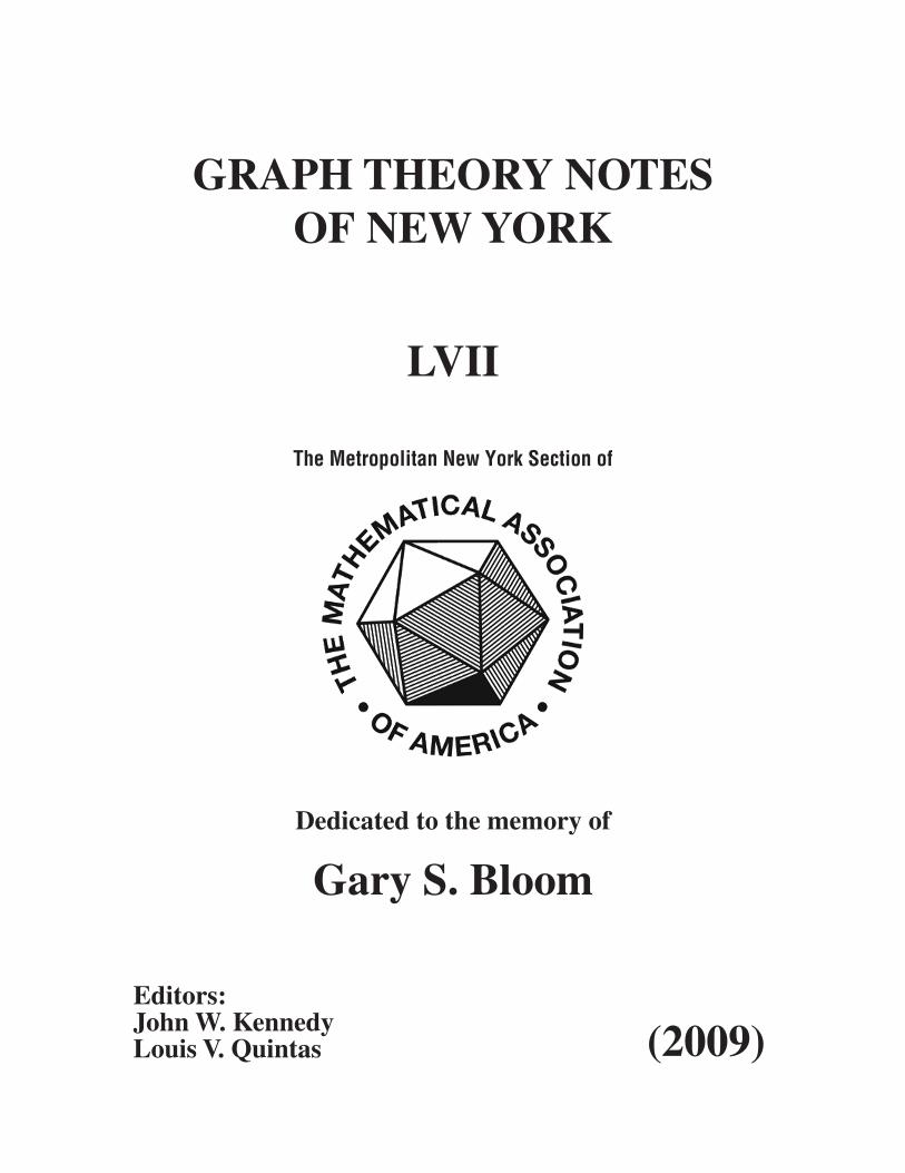
In this figure we have a robot at point S wanting to go to point E, needing to avoid some polygonal obstacles.One such path is shown and it is clear that one could find infinitely many others. Finding the shortest path insuch an infinite set can be much harder than optimizing over a finite set, but in this case we can readily reducethe set of possibilities to a finite one.
Imagine that the path shown in Figure 5 is a string and we pull on both ends of it to make the path shorter (seeSXYE in Figure 6). We arrive at a piecewise linear path whose endpoints and bendpoints are in the set that isthe union of and the set of vertices of the obstacles. This means that the shortest path can be found in
n 2⁄n 12=
Figure 4: An arrangement of curves with no two-sided region.
Figure 5: A mobile robot wants to go from start (S) to end (E).
S E,{ }
W. Meyer: The nature of graph theory: A visitor kibitzes 17
the visibility graph; that is, the graph whose vertices are the points just mentioned and whose edges are all seg-
ments that connect these points provided they do not pierce the interior of an obstacle.
Before we go any further, I should specify that the coordinates of S and E and those of all the obstacle corner
points are known. Furthermore, the sequence of points forming the boundary of each obstacle is also known.
This means that it is a fairly routine problem to compute the adjacency matrix of the visibility graph, and the
lengths of its edges.
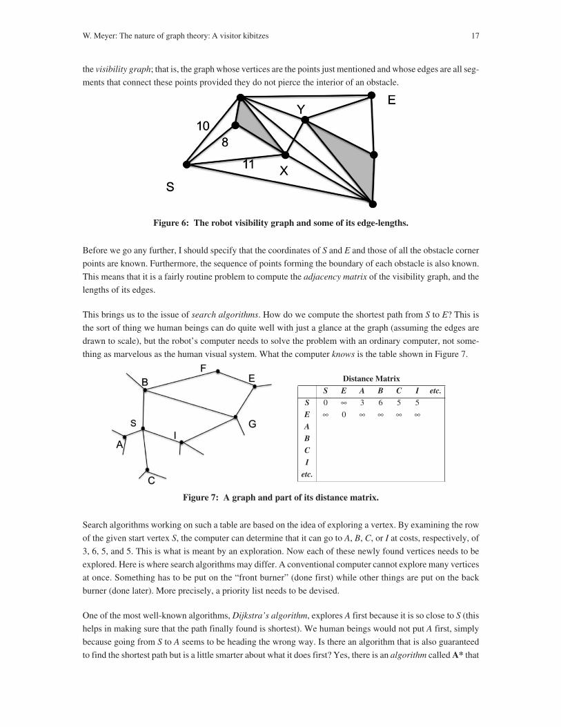
This brings us to the issue of search algorithms. How do we compute the shortest path from S to E? This is
the sort of thing we human beings can do quite well with just a glance at the graph (assuming the edges are
drawn to scale), but the robot’s computer needs to solve the problem with an ordinary computer, not some-
thing as marvelous as the human visual system. What the computer knows is the table shown in Figure 7.
Search algorithms working on such a table are based on the idea of exploring a vertex. By examining the row
of the given start vertex S, the computer can determine that it can go to A, B, C, or I at costs, respectively, of
3, 6, 5, and 5. This is what is meant by an exploration. Now each of these newly found vertices needs to be
explored. Here is where search algorithms may differ. A conventional computer cannot explore many vertices
at once. Something has to be put on the “front burner” (done first) while other things are put on the back
burner (done later). More precisely, a priority list needs to be devised.
One of the most well-known algorithms, Dijkstra’s algorithm, explores A first because it is so close to S (this
helps in making sure that the path finally found is shortest). We human beings would not put A first, simply
because going from S to A seems to be heading the wrong way. Is there an algorithm that is also guaranteed
to find the shortest path but is a little smarter about what it does first? Yes, there is an algorithm called A* that
Figure 6: The robot visibility graph and some of its edge-lengths.
Figure 7: A graph and part of its distance matrix.
Distance Matrix
S E A B C I etc.
S 0 ∞ 3 6 5 5
E ∞ 0 ∞ ∞ ∞ ∞A
B
C
I
etc.
18 Graph Theory Notes of New York LVII (2009)
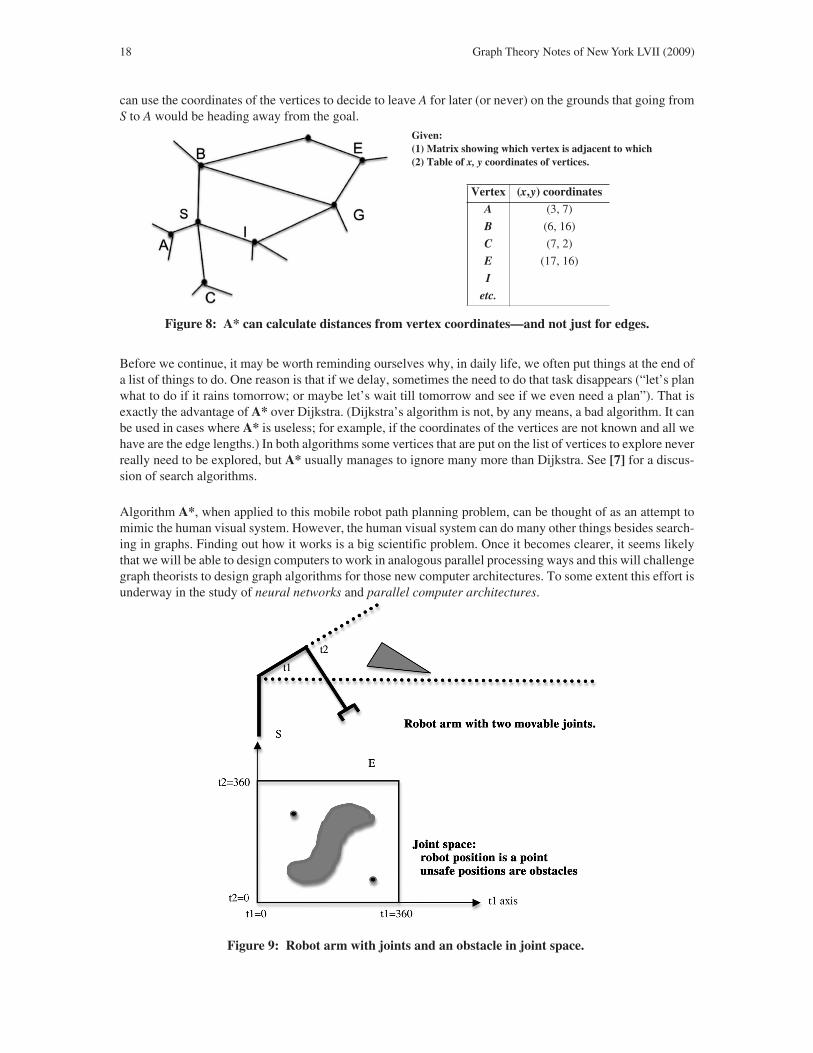
can use the coordinates of the vertices to decide to leave A for later (or never) on the grounds that going fromS to A would be heading away from the goal.
Before we continue, it may be worth reminding ourselves why, in daily life, we often put things at the end ofa list of things to do. One reason is that if we delay, sometimes the need to do that task disappears (“let’s planwhat to do if it rains tomorrow; or maybe let’s wait till tomorrow and see if we even need a plan”). That isexactly the advantage of A* over Dijkstra. (Dijkstra’s algorithm is not, by any means, a bad algorithm. It canbe used in cases where A* is useless; for example, if the coordinates of the vertices are not known and all wehave are the edge lengths.) In both algorithms some vertices that are put on the list of vertices to explore neverreally need to be explored, but A* usually manages to ignore many more than Dijkstra. See [7] for a discus-sion of search algorithms.
Algorithm A*, when applied to this mobile robot path planning problem, can be thought of as an attempt tomimic the human visual system. However, the human visual system can do many other things besides search-ing in graphs. Finding out how it works is a big scientific problem. Once it becomes clearer, it seems likelythat we will be able to design computers to work in analogous parallel processing ways and this will challengegraph theorists to design graph algorithms for those new computer architectures. To some extent this effort isunderway in the study of neural networks and parallel computer architectures.
Figure 8: A* can calculate distances from vertex coordinates—and not just for edges.
Given:(1) Matrix showing which vertex is adjacent to which(2) Table of x, y coordinates of vertices.
Vertex (x,y) coordinates
A (3, 7)
B (6, 16)
C (7, 2)
E (17, 16)
I
etc.
Figure 9: Robot arm with joints and an obstacle in joint space.

W. Meyer: The nature of graph theory: A visitor kibitzes 19
Is there any surprise that graph theory can help a mobile robot find its way? Perhaps not. Our analysis is justa matter of providing a road network (visibility graph) for the vehicle, and the fact that road networks are help-ful to vehicles is something everyone knows. What was surprising to me was that graph theory can help in get-ting an arm safely from one position to another. Suppose the arm in Figure 9 needs to go from a startingposition S (where the angles are t1 and t2) to an ending position E (not shown) without any part of the armbumping into the obstacle. Any position of the arm can be specified by its two joint angles t1 and t2. These twoangular values can be thought of as specifying a point in joint space (bottom of Figure 9), by which we meanthe set of all ordered pairs of these angles. (In this space 0 and 360 signify the same thing, and no valuesgreater than 360 need be considered, so our joint space is a square with opposite ends identified. (Thus jointspace is a torus topologically speaking, but this will not concern us in our high level overview.)
Now the points of joint space fall into two categories: safe points where the angles are such that the arm posi-tion does not intersect the obstacle, and unsafe points where the angles cause an intersection. The startingposition and ending positions correspond to safe points. What is wanted is a path from the starting safe pointto the ending safe point, avoiding all unsafe points. Now this sounds a lot like the mobile robot problem. I amsweeping a lot of interesting and tricky issues under the rug here, but the punch line of this path planning pro-cess is that we are back at the task of finding and analyzing a safe highway system (graph) for the point rep-resenting the arm to move along. I found this surprising when I became aware of it. Meyer and Benedict, in1988 gave a simple discussion of these ideas about robots.
4. DNA Sequencing and Overlap Digraphs
For my final example, I hark back to the 1990s when I was back in academia and my wife Rochelle and I wereteaching mathematics courses for general education audiences (also known as liberal arts mathematics). Wewere willing to try any material that used mathematics less sophisticated than calculus provided it had someinteresting application that might appeal to our often skeptical audience. One of the major scientific chal-lenges of the day was the Human Genome Project, the objective of which was to “read” the sequence of chem-icals making up a DNA (deoxyribonucleic acid) strand of a typical human being (DNA strands differ fromone person to the next—that is why some of us have blue eyes and others have other colors—but mostly wehuman beings are all the same in our DNA). To our surprise, graph theory arises here as well.
There are just four kinds of chemicals (called nucleotides or bases) making a up a DNA strand: they are sym-bolized by G, C, T, and A. It is their sequence that determines the kind of creatures we are biologically. Thesestrands are so long that present day technology makes it impossible to read the entire sequence.
However, shorter strands can be read. In the shotgun method we take a large number of such strands and applya random method of breaking them up. Each strand gets sliced up in its own way. How can we put themtogether? It is helpful to think of a single strand and its fragments. The problem is that we do not know whichfragment comes first, which comes second, and so forth. The problem is a little bit analogous to what youwould face if you had printed out an essay without page numbers and then dropped the pages. The solutionto the biochemical dilemma is a little analogous to what we would do to put our essay back together in properorder. Say you had a page that ended with the words “Napoleon and” and another that started with “Jose-phine”. It is a good guess that they go together. Here is one way to analyze what goes on in our minds—andwhat we will do with the DNA fragments. We have the following overlapping concepts in our minds:
NapoleonFamous couples in historyJosephine.
The middle concept overlaps the first and third and prompts us to think about the concept “Napoleon and Jose-phine”.
Figure 10: Two DNA strands wound around one another.

20 Graph Theory Notes of New York LVII (2009)
Now let us see how this might work with DNA. Before we dive in, it is important to be aware that what weare presenting here is extraordinarily simplified. The Human Genome Project required many millions of dol-lars and years of effort by people in a number of countries. What we are presenting here is the tip of a germof a hint of an idea of how graph theory can narrow down the possibilities for what the original chain sequencewas.
Figure 11 shows just three (normally there would be many) copies of a DNA strand split randomly. In thelower part of the figure we show all splits in one version of the strand. The horizontal bars indicate the frag-ments created by the split. Some of the fragments overlap. These fragments are floating around chaotically ina test tube as in Figure 12.
Even though these fragments are floating randomly we can go fishing and capture them and read the sequenceof each one we find, making a list of the different fragments we find. The next step is to remove from our listany fragment totally contained inside another. (These show no overlap and it is only the overlaps that help us.In fact containment can hinder the work.)
Now we create a table of all possible overlaps as in Figure 13. Some of these overlaps do not appear in theoriginal strand and this is why we call them possible overlaps. Our job is to select the right overlaps and usethem to stitch the strand back together.
Figure 11: Three shotgun splits of copies of the same DNA strand.
Figure 12: Three shotgun splits of copies of the same DNA strand.

W. Meyer: The nature of graph theory: A visitor kibitzes 21
From the overlap table we can make the overlap digraph where the fragments are the vertices and where wedraw an edge from one fragment to another if there is a non-zero entry in the overlap table in the row of thefirst fragment and the column of the second.
The next step is to consider these questions: how should we think about an edge with respect to stitching thefragments together; how should we think about a path? An edge is an overlap and it allows us to stitch togethertwo fragments (the vertices). (Leave aside for a moment whether it is a an erroneous stitching.) Adding a sec-ond edge to make a path of length two allows us to have three fragments stitched together. Since we are goingto need all the fragments, and without duplication, this means we should look for a Hamilton path.
Usually the start and end fragments can be determined. Of course there will usually be many Hamilton pathsfrom that start to that end. Scientists have discovered that the most likely true stitching is the one for whichthe extent of overlap is greatest. Thus we have a version of the travelling salesman problem:
Find the longest length Hamilton path in the overlap digraph.
Figure 13: The overlap table.
Figure 14: The overlap digraph.

22 Graph Theory Notes of New York LVII (2009)
Again, there may be many longest Hamilton paths. Furthermore, the principle about longer paths being morelikely is only a biochemical heuristic, not a guarantee. What it come down to is that finding the longest Hamil-ton path at best narrows the possibilities (but drastically!) and sometimes only points in the right generaldirection. More work, which we do not describe here, has to be done. (We did mention, did we not, that theHuman Genome Project took many years and heaps of money?)
For more on DNA sequencing: from the advanced point of view, see [8]–[10]. A simplified presentation wehave used for general education courses in mathematics may be found in [1].
5. Afterthoughts
So now let us step back and think about the big picture of graph theory. A graph is the most concrete of math-ematical objects. It is true one can think of it as a subset of a Cartesian product of sets, or perhaps as a topo-logical space, but what we always do when we are not being silly is to draw a picture. This concreteness hassometimes led other mathematicians to hold it in low regard. There was a time a few decades ago when oneheard it referred to as “the slums of topology.” This may have appealed to topologists because their subjecthad been the butt of criticism in the 1920s when topology was called “Geometry done by drunkards.”
As an aside, I cannot help mentioning that in the 1950s it was easy to criticize graph theory because there wasnot much of it, especially in relation to topology. However, as Figure 15 shows, things have changed quite abit. Graph theory has overtaken topology in quantity of research.
Now mathematics is not just about the number of papers, no matter what your tenure committee tells you.What my experiences in graph theory, as I have related them here, tell me is that graphs come up in surprisingcircumstances. All the best mathematics is like this, providing a way of thinking about diverse phenomena.(Consider, for example, the way topology provides structure for analysis as well as a new window for geom-etry.) However, you should not take the word of a kibitzer. Here are the words of a master of our subject,I.M. Gelfand, lecturing at the Courant Institute in 1990.
“The older I get, the more I believe that at the bottom of most deep mathematical problems there is a combinatorial problem.”
The importance of connection is also recognized outside of mathematics. The visionary environmentalistJohn Muir (1838–1914) said (well before this sentiment became popular):
“When one tugs at a single thing in nature; he finds it attached to the rest of the world.”
One can see a recognition of graph theory as an organizing idea in popular culture. In the 1980s, a local tele-phone company used a jingle involving the phrase “We’re all connected.” In the 1990s a game appeared basedon this concept, called the Kevin Bacon Game. The object of the game is to start with any actor/performer whohas been in a movie and then seek a path to Kevin Bacon (the well known actor) in the graph whose vertices
Figure 15: Slums versus geometry of drunkards (count of journal articles in Math Reviews.

W. Meyer: The nature of graph theory: A visitor kibitzes 23
are all individuals that have been in a movie and two actors are adjacent if and only if the have been in a movietogether. The smallest number of edges in a path linking an actor with Kevin Bacon is called the Bacon num-ber of the actor (see <http://oracleofbacon.org/help.php>). Of course the game was not described in this wayin popular culture, but it was clearly a shortest path problem in graph theory. I would be remiss if I did notmention that the Kevin Bacon Game has its analogy in the activity of determining the ErdŒs Number of anyindividual that has published a paper. Here one starts with an individual and looks for a shortest path to PaulErdŒs (there is no need to describe this icon of mathematics to readers of Graph Theory Notes of New York)in the graph whose vertices are all individuals that have published a paper and with two authors adjacent if andonly if they are coauthors. This graph is called the ErdŒs collaboration graph. The length of a shortest pathin this graph from an author to ErdŒs is called the ErdŒs number of the author (see <http://www.oak-land.edu/enp>). To illustrate the unbounded creativity of game constructors and graph theorists these twonumbers have been combined in the definition of the ErdŒs–Bacon number (see <http://en.wikipe-dia.org/wiki/Erdos-Bacon_number>), which is simply the sum of the ErdŒs number and the Bacon number.The first number is the collaborative distance relative to the activity of writing a paper and the second numbermeasures how separated relative to appearing in a film an individual is from Kevin Bacon. The ErdŒs–Baconnumber is a little more complex than each of its constituent numbers in that it combines two types of activity.Nevertheless, anyone checking out their three numbers is usually surprised at how small they turn out to beand how small their separations are from these two people.
In conclusion I would like to say that graph theory has many desirable characteristics: it is everywhere youlook and it is concrete enough that it has wide appeal for research and for teaching, even at the most basiclevel.
References
[1] R. Meyer and W. Meyer; Mathematics and the Currents of Change, Pearson Custom Publishing, 2nd ed., (2007).
[2] J.J. Sylvester; Mathematical question 11851, Educational Times, 59, 98 (1893).
[3] L.M. Kelly and W.O.J. Moser; On the number of ordinary lines determined by n points, Canad. J. Math., 10, 210–219 (1958).
[4] B. Grünbaum; Arrangements and Spreads, Conference Board of the Mathematical Sciences, Regional ConferenceSeries in Mathematics, Number 10, AMS (1972).
[5] G. Ringel; Teilungen der Ebene durch Geraden oder Topologische Geraden, Math. Z., 64, 79–102 (1956).
[6] G. Ringel; Über Geraden in Allgemeiner Lage, Elem. Math., 12, 75–82 (1957).
[7] B. Raphael; The Thinking Computer: Mind Inside Matter, W.H. Freeman & Company (1976).
[8] G. Hutchinson; Evaluation of polymer sequence fragment data using graph theory, Bull. Math. Biophysics, 31, 541–562 (1969).
[9] J.P. Hutchinson and H.S. Wilf; On Eulerian circuits and words with prescribed adjacency patterns, J. Comb. Theory(A), 18, 80–87 (1975).
[10] J. Setubal and J. Meidanis; Introduction to Computational Molecular Biology, PWS (1997).
Received: July 13, 2009
Graph Theory Notes of New York LVII, 24–28 (2009)The Mathematical Association of America.
[GTN LVII:3] THE TRAVELLING SALESPERSON PROBLEM: LET US PLAN A ROAD TRIP!
Ida KlikovacDepartment of Mathematics, Computer Science, and Information TechnologyNassau Community College, SUNYOne Education DriveGarden City, New York 11530, U.S.A.<[email protected]>
AbstractThis note offers ideas that are appropriate for exposing high school and freshman college students totopics in graph theory. A small instance of the traveling salesperson problem is introduced and stu-dents are guided to a method for solving this problem. Subsequent discussion is then used to encour-age students to explore broader issues related to larger instances of this kind of problem. Thepedagogical tactics described can be incorporated into a lesson plan, to suggest teaching techniques,or generally to offer suggestions to mathematics educators.
1. Objectives
The lesson “Let Us Plan a Road Trip!” described here is designed to introduce high school and freshman col-lege students to travelling salesperson problems in a way that successfully motivates and excites studentsabout studying a graph theory concept [1]. Students are asked the initial question: Given a small (finite) num-ber of cities together with the cost of travelling between each pair of cities, what is the least expensive wayto visit all the cities and eventually return to the starting city.
“Let Us Plan a Road Trip!” was designed as a three-part presentation. The length of each part can varydepending on the preparation of the students and the style of the instructor. The presentation can be made inas few as one meeting or as many as three sessions.
1. An introduction to tours in graphs in the form of Hamilton cycles and the closely related travelling salesperson problem.
2. A session for students to engage in interactive learning in small groups, through discussion of the content of Part 1 and extending their knowledge of the topic by means of Internet search activities.
3. A class discussion session to obtain feedback from students and their reflections on the lesson content. At this stage the students should be sufficiently prepared to make extensive use of Internet resources to locate and follow up on the vast amount of information that is available on this topic.
2. Introduction to Tours in Graphs
Four cities are suggested: New York (NY), Boston (BOS), Washington D.C. (DC), and Orlando (ORL). Thestudents are then asked to design a road trip to start from NY, visit each of the other three cities, and thenreturn to NY. The goal is to do this in the most efficient way. Specifically, the aim is to determine (1) the jour-ney with the shortest total distance, and (2) the least expensive route that visits all the cities and returns to NY.Clearly, the objectives minimize two closely related quantities: distance and cost.
To guide students toward a procedure (not necessarily the most efficient) for obtaining the optimal four-citysolution, a tree diagram can be used to visually display all the possible ways to visit each city starting in andreturning to NY. The six possible routes are labeled numerically 1–6 to emphasize the number of possibilitiesand to refer to particular route(s) later in the lesson. (See Figure 1.)

I. Klikovac: The travelling salesperson problem: Let us plan a road trip! 25
Since the problem needs to compute the total length of each possible route, a table of distances between pairsof cities is also provided, as shown in Table 1.
For students that have little or no prior knowledge of graphtheory, time needs to be spent to introduce an appropriatetype of graph for these problems; namely, a weighted com-plete graph. Additionally, appropriate terminology must bedeveloped to aid with discussion of the problem and its solu-tion: a vertex to represent each city, an edge to represent thedirect route between the pair of cities it connects, an edgeweight to represent the distance in miles along the route con-necting two cities. For the problem under consideration, thisleads to the weighted complete graph shown in Figure 2.
Table 1: Intercity distances in miles.
NY (NCC) BOS DC ORL
NY (NCC) 183 209 943
BOS 183 392 1113
DC 209 392 758
ORL 943 1113 758
Figure 1: Tree diagram for possible routes.
NY
BOS
ORL
DC
183
1113758
209
392
943
Figure 2: Weighted complete graph.

26 Graph Theory Notes of New York LVII (2009)
The next activity is to get the students to compute the total distance for each of the possible routes shown inFigure 1. Thus, for example, for Route 1 (NY–BOS–DC–ORL–NY) the total distance is
miles.
This leads to the results shown in the second column of Table 2.
To save money a gasoline efficient car should be used to make the journey. We suggested that a hybrid carthat attains 50 m.p.g. Then for Route 1 the gasoline consumption would be gallons. Theresults for each possible route are shown in the third column of Table 2. For each of the possible routes
Finally, to compute the cost of each trip one can use a gasoline price of $3.00/gallon, to obtain the cost foreach possible route as shown in the final column of Table 2.
Table 2 shows that Routes 2 and 4 (shown boldface)are both optimal routes (shortest total distance, leastgasoline consumption, smallest cost). These tworoutes of course result in the smallest cost ($135.78)suggesting that the trip should be planed in one of thetwo ways:
NY–BOS–ORL–DC–NY or
NY–DC–ORL–BOS–NY.
These two solutions, of course, represent the samecycle taken in opposite directions. The optimalroute(s) can be nicely illustrated after removingunused edges from the original weighted graph asshown in Figure 3.
To close the introductory session on graphs and the travelling salesperson problem, I choose to introduceWilliam Rowan Hamilton and his contributions to graph theory; explaining how Hamilton introduced thetopic of what are now called Hamilton cycles in graphs. This topic then involved many subsequent authors toconsider algorithms for locating optimal Hamilton cycles in weighted graphs, a topic known as the travellingsalesperson problem. Although no efficient (that is, polynomial) algorithm for the travelling salespersonproblem is known, the search for efficient algorithms that locate better suboptimal solutions continues.
3. Group Learning
In the second stage of this presentation, students are encouraged to engage in discussion in small groups mak-ing use of the Internet to extend their knowledge of the ideas previously introduced. It is suggested theychoose a (not too large) collection of cities for themselves and calculate optimal Hamilton cycle solutions.They should be encouraged to elaborate on their reasons for selecting a particular collection of destinations,
Table 2: Total distance, gasoline consumption, and cost for each route.
Routenumber
Total distance (miles)
Gasoline consumption(gallons)
Total cost ($)
1 2276 45.52 136.56
2 2263 45.26 135.78
3 2657 53.14 159.42
4 2263 45.26 135.78
5 2657 53.14 159.42
6 2276 45.52 136.56
183 392 758 943+ + + 2276=
2276 50⁄ 45.52=
NY
BOS
ORL
DC
183
1113758
209
Figure 3: Graph of optimal solution.

I. Klikovac: The travelling salesperson problem: Let us plan a road trip! 27
thereby promoting their appreciation of the uses of mathematics [2] . They are asked to draw conclusions andwrite a brief report for later reflection.
4. Discussion
After the period of work in small groups, it is worthwhile to allow students time to reflect on successfullycompleted tasks and to share results with each other, explaining the reasoning they used in obtaining optimaltours and other discoveries they made while working in small groups.
It also seems useful to close the session by posing open questions that could lead students to discover addi-tional facts about the travelling salesperson problem. This stimulates thinking and keeps new material freshin their minds. Among the questions asked, and the student replies, were the following:
Who in real life benefits from the discoveries about the travelling salesperson problem?
One student suggested that this would be useful for musicians who are touring with their bands all over thecountry,
Why is there no formula or “efficient” algorithm that provides an exact solution to the travelling salesperson problem?
What does suggest for large n?
One student (after typing a large number for n in a TI84 graphing calculator said: “I got an overflow!
Even for relatively modest values of n the number Hamilton cycles in a complete graph with n ver-tices (cities) that start and end at a particular city, is too large for a calculator to compute.
Why did we get exact reversals in a complete weighted graph, a mirror image?
One student observed that Route 2 is the exact reverse of Route 4, it is the same city order taken backward.“Is this always the case?”
“The history of graph theory has been closely linked to applications, witness for examplethe importance of computer science, chemistry and electrical networks in the developmentof the subject. It seems reasonable to expect that applied problems will continue to play animportant role, both in stimulating new graph-theoretical work and as areas where graphtheory can be of practical use.” — F.S. Roberts [3]
Discussion of this kind continued for quite a while.
5. Reflection
The travelling salesperson problem has always been one of my personal favorite topics in graph theory. Thefact that mathematicians have not been able to find an efficient method to solve it nor have they been able toprove that one does not exist is as fascinating to me as it is to any mathematics enthusiast. It was for this reasonthat I choose to explore the travelling salesperson problem with my high school students using a rather untra-ditional teaching style I call: learning while having fun.
This session described here could be extended by introducing brute force methods and nearest neighbor algo-rithms. Interactive learning could continue by assigning take home projects, making full use of the Internet,in which students can significantly increase the number of vertices (cities) and make use of approximate algo-rithms that (efficiently) result in suboptimal solutions that are sufficiently close to the exact solution that theycan be used in practical applications.
An additional research project that could be offered (extra credit) could encourage students to explore factsabout the travelling salesperson problem. Having them write a short paper on what they think makes the trav-elling salesperson problem impossible to solve.
Mathematics educators have the power to inspire students by being creative in their teaching styles, connect-ing the material they introduce to the interests of their students, and relate this material to “real world” appli-cations.
The ideas described in this note reflect my notions about one way to accomplish this.
n 1–( )!
n 1–( )!

28 Graph Theory Notes of New York LVII (2009)
References [1] National Research Council; Everybody Counts: A Report to the Nation on the Future of Mathematics Education,
Board on Mathematical Sciences and Mathematical Sciences Education Board, Washington, D.C., National Acad-emy Press (1989).
[2] P.Z. Chinn; Discovery method teaching in graph theory. In Quo Vadis Graph Theory? A Source Book for Challengesand Directions, J. Gimbel, J.W. Kennedy, and L.V. Quintas, Editors; Elsevier Science Publishers, Annals of DiscreteMathematics, 55, 375–384 (1993).
[3] F.S. Roberts; New directions in graph theory (with an emphasis on the role of applications). In Quo Vadis Graph The-ory? A Source Book for Challenges and Directions, J. Gimbel, J.W. Kennedy, and L.V. Quintas, Editors; Elsevier Sci-ence Publishers, Annals of Discrete Mathematics, 55, 13–44 (1993).
Received: August 6, 2009Revised: November 24, 2009

Graph Theory Notes of New York LVII, 29–33 (2009)The Mathematical Association of America.
[GTN LVII:4] SOME QUESTIONS ON GRAPH PROTECTION
William F. KlostermeyerSchool of ComputingUniversity of North FloridaJacksonville, FL 32224-2669, U.S.A.<[email protected]>
1. Introduction
Let be a graph with n vertices. A number of recent papers have considered problems associatedwith using mobile guards to defend G against an infinite sequence of attacks; see for instance [1]–[6].
Denote the open and closed neighborhoods of a vertex by and , respectively. That is,
and
A dominating set of G is a set with the property that, for each , there exists adjacentto u. The minimum cardinality among all dominating sets is the domination number . A total dominatingset of G is a set with the property that, for each , there exists adjacent to u. The minimumcardinality among all total dominating sets is the total domination number . Note that this is onlydefined for graphs with no isolated vertex.
A vertex cover of G is a set such that, for each edge at least one of u or v is in C. Let be the vertex cover number of G; that is, the minimum number of vertices required to cover all edges of G. Atotal vertex cover of G is a vertex cover with the property that, for each , there exists adjacent to u. The minimum cardinality among all total vertex covers is the total vertex cover number .
An independent set of G is a set with the property that no two vertices in I are adjacent. The maximumcardinality amongst all independent sets is the independence number . For all connected graphs G oforder n, it is known that .
Let , , be a set of vertices with one guard located on each vertex of Di; at most one guard can belocated on a vertex. Each problem is modeled as a two-player game: The defender chooses D1 as well as Di,
, and the attacker chooses the locations of the attacks . Thus, the location of an attack can bechosen by the attacker depending on the location of the guards. Each attack is handled by the defender bychoosing the next Di subject to constraints. The defender wins the game if they can successfully defend anyseries of attacks, subject to the constraints of the game; the attacker wins otherwise.
For the eternal dominating set problem, , , is required to be a dominating set, (assume, with-out loss of generality, ), and is obtained from Di by moving one guard to ri from a vertex
, . The size of a smallest eternal dominating set for G is denoted by .
For the m-eternal dominating set problem, Di, , is required to be a dominating set, (assume, with-out loss of generality ), and is obtained from Di by moving guards to neighboring vertices. Thatis, each guard in Di may move to an adjacent vertex. It is required that . The size of a smallest m-eternal dominating set for G is denoted by .
For the m-eternal vertex covering problem, Di, , is required to be a vertex cover, , and isobtained from Di by moving guards to neighboring vertices. That is, each guard in Di may move to an adjacentvertex. It is required that in moving from Di to that a guard move along edge ri. The size of a smallestm-eternal vertex cover for G is denoted .
The total versions of the three parameters defined above are defined in an obvious manner, and denoted by, , and , respectively.
G V E,( )=
x V∈ N x( ) N x[ ]
N x( ) v : xv E∈{ }= N x[ ] N x( ) x{ }.∪=
D V⊆ u V D–∈ x D∈γ G( )
X V⊆ u V∈ x X∈γ t G( )
C V⊆ uv E∈ α G( )
C V⊆ u C∈ x C∈αt G( )
I V⊆β G( )
n β G( )– α G( )=
Di V⊂ 1 i≤
i 1> r1 r2 …, ,
Di 1 i≤ ri V∈ri Di∉ Di 1+
v Di∈ v N ri( )∈ γ ∞ G( )
1 i≤ ri V∈ri Di∉ Di 1+
ri Di 1+∈γm
∞ G( )
1 i≤ ri E∈ Di 1+
Di 1+αm
∞ G( )
γ t∞ G( ) γmt
∞ G( ) αmt∞ G( )

30 Graph Theory Notes of New York LVII (2009)
2. Basic Bounds and Questions
Let be the clique covering number of G; that is, . The following result is from [3].
It is shown in [4] that . Likewise, from [7] we have the following.
It is known that if and only if [5]. A characterization of graphs with was given in [8].
Question 1 [3]: (1) For which graphs is ?(2) For which graphs is ? �
It was proved in [1] that for all series-parallel graphs G. The question remains open for pla-nar graphs.
Theorem 1: For all connected graphs G, , with equality if and only if , .
Proof: Given a minimum vertex cover, C, of G with cardinality k, we form a total vertex cover of size at most2k as follows. For each , if v has no neighbor in C, choose an edge uv that v covers and add u to the newvertex cover. It is clear that and .
For the other direction, assume , which implies . Consider a minimum vertex cover, C, ofG with cardinality k. If there are two adjacent vertices in C, then the process described above will produce atotal vertex cover of size less than 2k. Likewise if there exists a pair of vertices such that
. Otherwise, for all and there exists an edge that is uncovered.�
Question 2: For which graphs G is ? �
A neo-colonization is a partition of the vertex set of graph G such that each Vi induces aconnected graph. A part Vi is assigned a weight of 1 if it induces a clique and otherwise, where
is the size of the smallest connected dominating set in the subgraph induced by Vi. (A connecteddominating set of G is a set D such that D is a dominating set and is connected.) Then is the min-imum weight of any neo-colonization of G. is called the clique-connected cover number of G. Goddardet al. [3] defined this parameter and proved that .
Theorem 2 [5]: Let T be a tree. Then . �
Question 3: For which graphs G is ? �
Although the clique-connected cover number is a sometimes better bound on the m-eternal domination num-ber than the independence number, it is not always. C5 is a simple example. An infinite family of additionalexamples is now constructed. Let G be a connected graph with girth k and chromatic number k (k large). ThusG has clique size equal to two. Then the complement of G, , has independence number two and clique covernumber k. In order for to have clique-connected cover number 2 it must be that it has connected dominationnumber 1; that is, it has a vertex of degree . This is not possible since G is connected.
Theorem 3: Let G be a connected graph with n vertices. Then , with equality for , , and other graphs.
Sketch of Proof: Let T be a spanning tree of a graph G with order n. One can prove by induction that. One way to proceed with the inductive step is to consider two cases: (1) if each leaf u is such
that its only neighbor v is adjacent to exactly one leaf (in which case we can delete u and consider the casesdepending upon what the vertices close to v look like) and (2) if there exists a leaf such that its neighbor isadjacent to at least two leaves (delete the two leaves and proceed by induction). �
θ G( ) θ G( ) χ G( )=
γ G( ) γm∞ G( ) β G( ) γ ∞ G( ).≤ ≤ ≤
γ ∞ G( ) β G( ) 1+2⎝ ⎠
⎛ ⎞≤
γ G( ) α G( ) αm∞ G( ) 2α G( ).≤ ≤ ≤
γ ∞ G( ) γ G( )= γ G( ) θ G( )=γ G( ) α G( )=
γ ∞ G( ) θ G( )=γ ∞ G( ) α G( )=
γ ∞ G( ) θ G( )=
αt G( ) 2α G( )≤G K1 m,= m 1≥
v V∈α K1 m,( ) 1= αt K1 m,( ) 2=
G K1 m,≠ α G( ) 1>
u v, C∈dist u v,( ) 2= dist u v,( ) 2> u v, C∈
αt G( ) α G( )=
V 1 V 2 … V t, , ,{ }1 γ c G V i[ ]( )+
γ c G V i[ ]( )G D[ ] θc G( )
θc G( )γm
∞ G( ) θc G( )≤
θc T( ) γm∞ T( )=
θc G( ) β G( )≤
GG
n 1–
γm∞ G( ) n 2⁄≤
C4 P2n 1+
θc T( ) n 2⁄≤

W.F. Klostermeyer: Some questions on graph protection 31
Question 4: (1) For which graphs G is ?
(2) For which graphs G is ?
(3) For which graphs G is ?
(4) For which graphs G is ? �
Question 5: (1) For which graphs G is ?
(2) For which graphs G is ? [6] �
We initially thought that a graph G must have to satisfy , for example C4 and .However, this is not the case because there are several small graphs having : and . Likewise, has .
3. Edge Protection
Let , or L when the context is clear, denote the number of leaves of a tree T. A stem is a vertex adjacentto a leaf (we assume that stems have degree greater than one, otherwise we have a component of G that is iso-morphic with K2). Let be the set of stems of G. It is shown in [7] that for all graphs Gand the same paper characterized the infinitely many graphs where equality is attained. The next two resultscan be proved using identical techniques to those used in [7] to obtain analogous results about the m-eternalvertex cover.
Theorem 4: For all connected graphs G, . �
Theorem 5: For any tree T, . �
Question 6: For which graphs other than and P5 is the bound in Theorem 4 sharp? �
Question 7: For which graphs G is ? �
Theorem 6: Let G be a connected graph with more than two vertices.Then .
Proof: Let a connected graph G have at least three vertices. Consider a minimum clique cover of G. For eachK1 in this clique cover, attach the K1 as a pendant vertex to an adjacent clique, thereby forming a partition Pof G consisting of cliques and cliques with pendant vertices. Observe that for
and the total m-eternal vertex cover number of a clique with pendant vertices is equal its m-eternal ver-tex cover number (if this graph is not a K2). Place guards on the vertices of a minimum m-eternal vertex coverof G. Add additional guards so that each part in P contains at least two guards; thus the guards induce a totalvertex cover. We can defend attacks with this initial arrangement of guards while maintaining a total vertexcover: basically emulate the movement of guards in a minimum m-eternal vertex cover algorithm (that is,keep a guard at time t at each vertex on which the minimum m-eternal vertex cover algorithm has a guard attime t). Although sometimes guards on opposite ends of an edge must swap locations if that edge is attacked,it is not necessary for us to move a guard from u to v if there is already a guard at v and uv is not the attackededge (in which case the minimum m-eternal vertex cover algorithm might be moving a guard from u to anunoccupied vertex v).
This procedure uses less than guards unless P contains only K2 and , , cliques. If G con-tains a part, then there must be at least two guards in it at some point in time, as well as one guard ineach K2 at all times. On the other hand, if P contains only K2 parts, then G is bipartite with equal-sized partsand it is not hard to show the bound holds for such bipartite graphs. �
Question 8: For which graphs G is ? �
We believe the graphs satisfying Question 8 may fall into three classes: (1) K2, C4, and graphs of the form (that is, the corona of a graph H with K1); (2) trees with ; and (3) certain trees
with some edges or vertices replaced by C4 subgraphs.
γm∞ G( ) γ G( )=
γm∞ G( ) θc G( )=
γm∞ G( ) β G( )=
γm∞ G( ) n 2⁄=
γmt∞ G( ) γ G( )=
γmt∞ G( ) γ t G( )=
γ G( ) 2= γmt∞ G( ) γ G( )= C6
2
γmt∞ G( ) γ G( ) 3= = C3 C3×
P3 C3× P4 C3× γmt∞ G( ) γ G( ) 4= =
L T( )
S G( ) αm∞ G( ) 2α G( )≤
αmt∞ G( ) 2α G( )≤
αmt∞ G( ) V L– 1+=
K1 m,
αm∞ G( ) αmt
∞ G( )=
αmt∞ G( ) 2αm
∞ G( )<
αmt∞ Kn( ) n 1– αm
∞ Kn( )= =n 2>
2αm∞ G( ) K1 m, m 1>
K1 m,
αm∞ G( ) γm
∞ G( )=
H �K1 V L T( )– 1+ θc G( )=

32 Graph Theory Notes of New York LVII (2009)
Question 9 [7]: For which graphs is ?Are the two parameters equal for vertex-transitive graphs? �
Question 10 [7]: Let G and H be graphs such that and .Is it true that ?Does equality hold if we place no restrictions on H? �
Theorem 7: Let G be a connected graph. Then if and only if .
Proof: The equation obviously holds for K2 and C4. Suppose . First, suppose G contains apendant vertex v. Let . Let G be a smallest graph with these properties. If necessary, by attackingedges we can force a guard to be on v. Suppose the configuration of guards, with a guard on v, is a vertexcover, C, of G with size . Then is an eternal vertex cover, and by our assumptions, is also adominating set of , since an eternal vertex cover must always keep a guard on either u or v. If
contains a pendant vertex, we have a smaller counterexample; otherwise the argument belowapplies.
It is known that if G has no pendant vertex and , then G is a bipartite graph with vertex parts Aand B, see [8]. Then . First, suppose . If , G is con-nected and bipartite with no pendant vertices, it is known that . On the other hand, if ,then one can prove by induction on (see (�) below) that any connected bipartite graph G with satisfies . �
(�) Base cases of are easy. Assume and suppose we can protect G with guards. Let uand v be vertices such that is connected: For example, a leaf v from a spanning tree T of G and itsadjacent stem u from T. By the inductive hypothesis, we must have at least guards in at somepoint in time. Since , we must always keep a guard on at least one of . Hence, guardsare needed.
Theorem 8: Let G be a graph with no isolated vertex. Then if and only if Gis formed from a graph H, , by attaching pendant vertices to vertices of H in sucha way that the resulting graph does not contain adjacent vertices that are not stems and suchthat every stem is adjacent to at least one other stem.
Proof: Assume without loss of generality that G is connected. Suppose G is as described in the statement ofthe theorem. It is easy to see that .
Now suppose . It is known that if G is leafless, then if and G is a bipartite graphwith vertex parts A and B [8]. However, in this case, and .Hence, we may assume that G contains leaves. Note that if , then and .
In order for , it must be that has no pendant vertex [8]. Hence, we may focus atten-tion on such graphs. Consider the graph . When deleting stems and their neighbors, an edge uv willbe in the graph if both ends of the edge are not stems (although the vertices u and v may be deleted).For example, in P6, consists of one edge with no end vertex. Then, must not containedges with no end vertices. Furthermore, since is leafless, by the discussion above, mustbe bipartite. It follows that would have to consist only of isolated vertices and that these isolatedvertices are not in any minimum dominating set (and thus not in any minimum total vertex cover). Therefore,it must be that each stem has a neighboring stem, in order for a minimum vertex cover to be a total vertexcover. �
Question 11: For which graphs G is ? �
One might suspect that implies . However, consider C4 with one pendant ver-tex v attached to one of the vertices of the cycle. This graph G has , but and
. On the other hand, and .
αm∞ G( ) α G( )=
αm∞ G( ) α G( )= αm
∞ H( ) α H( )=αm
∞ G H×( ) α G H×( )=
αm∞ G( ) γ G( )=
G C4 K2,{ }∈
αm∞ G( ) γ G( )=
u{ } N v( )=
γ G( ) C v{ }–G u v,{ }–
G u v,{ }–
γ G( ) α G( )=γ G( ) min A B,{ }≤ αm
∞ G( ) A B= = G C4 K2,{ }∉γ G( ) n 2⁄< A B<
A A B<αm
∞ G( ) A 1+≥
1 A 2≤ ≤ A 2> AG u v,{ }–
A G u v,{ }–uv E∈ u v,{ } A 1+
γ G( ) αt G( )=V H( ) 1>
γ G( ) αt G( ) S G( )= =
γ G( ) αt G( )= γ G( ) α G( )=γ G( ) min A B,{ }≤ αt G( ) min A B,{ } 1+≥
V H( ) 1= γ G( ) 1= α G( ) 2=
γ G( ) α G( )= G N S[ ]–G N S[ ]–
G N S[ ]–G N S[ ]– G N S[ ]–
G N S[ ]– G N S[ ]–G N S[ ]–
γ t G( ) αt G( )=
α G( ) γ G( )= γ t G( ) αt G( )=α G( ) γ G( ) 2= = γ t G( ) 2=
αt G( ) 3= γ K3( ) α K3( )< γ t K3( ) αt K3( )=

W.F. Klostermeyer: Some questions on graph protection 33
Theorem 9: For all graphs G with no isolated vertex, .
Proof: By Theorem 8 we need only consider the types of graphs described there. Clearly, ,so we can focus on graphs with pendant vertices and stems. In such a graph, the only way to have is for the minimum total vertex cover to consist of the set of stems. However, if there is an attack on an edgeincident to a pendant vertex, we must move a guard there. �
Acknowledgement
The authors thank an anonymous referee for carefully reading the paper and offering valuable suggestions,including the provision of simplified examples.
References [1] M. Anderson, C. Barrientos, R. Brigham, J. Carrington, R. Vitray, and J. Yellen; Maximum demand graphs for eternal
security, J. Combin. Math. Combin. Comput., 61, 111–128 (2007).
[2] A.P. Burger, E.J. Cockayne, W.R. Gründlingh, C.M. Mynhardt, J.H. van Vuuren, and W. Winterbach; Infinite orderdomination in graphs, J. Combin. Math. Combin. Comput., 50, 179–194 (2004).
[3] W. Goddard, S.M. Hedetniemi, and S.T. Hedetniemi; Eternal security in graphs, J. Combin. Math. Combin. Comput.,52, 169–180 (2005).
[4] W.F. Klostermeyer and G. MacGillivray; Eternal security in graphs of fixed independence number, J. Combin. Math.Combin. Comput., 63, 97–101 (2007).
[5] W.F. Klostermeyer and G. MacGillivray; Eternal dominating sets in graphs, J. Combin. Math. Combin. Comput., 68,97–111 (2009).
[6] W.F. Klostermeyer and C.M. Mynhardt; Eternal total domination in graphs, Ars Comb., (2009) —to appear.
[7] W.F. Klostermeyer and C.M. Mynhardt; Edge protection in graphs, Australisian Journal of Combinatorics, 45, 235–250 (2009).
[8] B. Hartnell and D. Rall; A characterization of graphs in which some minimum dominating set covers all the edges,Czeck. Mathematical Journal, 45, 221–230 (1995).
Received: March 9, 2009Revised: November 12, 2009
γ G( ) αmt∞ G( )<
γ K2( ) αmt∞ K2( )<
γ αmt G( )<
Graph Theory Notes of New York LVII, 34–38 (2009)The Mathematical Association of America.
[GTN LVII:5] ON TWO CONJECTURES ABOUT FAULTY HYPERCUBES
Nelson Castañeda,1 Vasil S. Gochev,2 Ivan Gotchev,1 and Frederic Latour11Department of Mathematical SciencesCentral Connecticut State University1615 Stanley StreetNew Britain, CT 06050, U.S.A.<[email protected]><[email protected]><[email protected]>
2Department of MathematicsTrinity College300 Summit StreetHartford, CT 06106, U.S.A.<[email protected]>
AbstractLet F be a set of vertices in the binary hypercube Qn. A set F′ of vertices in Qn is a disjoint mirror twinof F if F′ has the same cardinality as F, , and the number of even vertices in F is equalto the number of odd vertices in F′. In this paper the following two results are proved. The first (seeTheorem 5), is a weaker version of Locke’s conjecture: The binary hypercube Qn with f deleted ver-tices of each parity is Hamiltonian if . The second (see Theorem 6), is a weaker version ofthe Castañeda–Gotchev conjecture: If , , and F is a set of f even and f odd verti-ces of Qn, then for every pair of vertices with opposite parity there exists a Hamil-tonian path in .
1. Introduction and Definitions
The n-dimensional hypercube Qn is the graph whose vertices correspond with the binary sequences of lengthn and whose edges connect pairs of vertices whose binary sequences differ in exactly one position. A givenvertex is called even if it has an even number of 1 bits in its binary representation; otherwise the vertex iscalled odd.
Given a graph and a set of vertices , the subgraph of G induced by S is the graphwhose vertex set is S and whose edge set consists of all edges in whose endpoints are both in S. Wedenote by the subgraph of G induced by the vertex set . Throughout this paper, we say that avertex u is a neighbor of a vertex v if u and v are adjacent in Qn.
Locke's conjecture [1] states that the binary hypercube Qn with f deleted vertices of each parity is Hamiltonianif . In 2003, S.C. Locke and R. Stong published a proof of this conjecture for the case [2].In [3] Castañeda and Gotchev proved the conjecture for each (for related results see [4]).
In the same paper the following conjecture was stated (see [3], 6.3) and verified for each and each: Let and . If F is a set of f even and f odd vertices of Qn, then for every pair of
vertices with opposite parity there exists a Hamilton path in from u to v.
Here, we formulate and prove weaker forms of the above two conjectures. We need the following definition.
Definition 1: Let F be a set of vertices in Qn. We say that a set F′ of vertices in Qn is amirror twin of F if F′ has the same cardinality as F, the number of even vertices in F is equalto the number of odd vertices in F′, and there is the same number of even and odd verticesin . In the case when , we call F′ a disjoint mirror twin of F. �
Using the terms defined above, Locke's conjecture can be restated as follows.
F F ′∩ ∅=
n f 2+≥n 3≥ 0 f n 3–≤ ≤
u v, V Qn F–( )∈Qn F–
G V E,( )= S V G( )⊂E G( )
G S– V G( )\S
n f 2+≥ f 1=f 4≤
f 2≤n f 3+≥ n 3≥ 0 f n 3–≤ ≤
u v, V Qn F–( )∈ Qn F–
F F′∩ F F′∩ ∅=
N. Castañeda, V.S. Gochev, I. Gotchev, and F. Latour: On two conjectures about faulty hypercubes 35
Conjecture 2 (Locke): Let and F be a set of vertices in Qn of cardinality. Then, for every disjoint mirror twin F′ of F the graph
is Hamiltonian. �
The following conjecture sounds more general than Locke's conjecture but is actually equivalent to it.
Conjecture 3: Let and F be a set of vertices in Qn of cardinality . Then for every mirror twin F′ of F the graph is Hamiltonian. �
Using the same terminology, the Castañeda–Gotchev conjecture can be reformulated as follows.
Conjecture 4: Let and F be a set of vertices in Qn of cardinality .Then for every pair of vertices with opposite parity and every mirror twin F′ of F with , there exists a Hamiltonian path in from u to v. �
It is easy to verify that the conjecture obtained from Conjecture 4 by replacing every mirror twin with everydisjoint mirror twin is equivalent to Conjecture 4.
In this paper, we prove the following theorem, which is weaker than Locke's conjecture since it follows fromit but does not imply Locke’s conjecture.
Theorem 5: Let , , and F be a set of vertices in Qn of cardinality f. Thenthere exists a disjoint mirror twin F′ of F such that the graph is Hamiltonian.
Since Theorem 5 follows from Locke's conjecture, which is true for each and each , we needto prove Theorem 5 only for and . In the proof we use the following theorem, which is aweaker form of the Castañeda–Gotchev conjecture, and therefore, is known to be true for each and each
.
Theorem 6: Let , , and F be a set of vertices in Qn of cardinality f. Thenfor every pair of vertices with opposite parity there exists a disjoint mir-ror twin F′ of F, with such that there exists a Hamiltonian path in
from u to v.
2. Proof of Theorem 6
As mentioned above, Theorem 6 is true for each and each . We continue the proof by induc-tion on f. Let and suppose that the claim is true for each and each . We prove theclaim for and every . Note that since we have .
Let and . Also let F be a set of vertices in Qn of cardinality f and be a pairof vertices with opposite parity.
Since , there must be a coordinate for which not all vertices of F agree. Suppose, without loss of gen-erality, that it is the first coordinate. For , let Vi be the subset of consisting of the verticeswhose first coordinate is i. Then for . Furthermore, since , one of
or must be at least two. Suppose, without loss of generality, that . Then theremust be a coordinate, other than the first, where not all vertices of agree. Without loss of generality,suppose that it is the second coordinate. For , let be the subset of consisting of thevertices whose first two coordinates are ij, and let . Since , , and all contain atleast one vertex of F, then for all .
Now, for , let be the subgraph of Qn induced by . Then each is an -dimen-sional hypercube, and since , we can apply the induction hypothesisfor each pair of vertices of opposite parity in .
Case 1: .
According to the induction hypothesis, applied to , there exists a disjoint mirror twin of , with , such that there exists a Hamiltonian path γ in
from u to v. The length of γ is . Since , then
.
n 2≥0 f n 2–≤ ≤ Qn F F′∪( )–
n 2≥ 0 f n 2–≤ ≤Qn F F′∪( )–
n 3≥ 0 f n 3–≤ ≤u v, V Qn F–( )∈
u v,{ } F′∩ ∅= Qn F F′∪( )–
n 2≥ 0 f n 2–≤ ≤Qn F F′∪( )–
f 4≤ n f 2+≥n 7≥ 5 f n 2–≤ ≤
f 2≤n f 3+≥
n 3≥ 0 f n 3–≤ ≤u v, V Qn F–( )∈u v,{ } F′∩ ∅=
Qn F F′∪( )–
f 2≤ n f 3+≥f 0 3≥ f f 0< n f 3+≥
f f 0= n f 3+≥ f 3≥ n 6≥f f 0= n f 3+≥ u v, V Qn F–( )∈
f 3≥i 0 1,{ }∈ V Qn( )
1 V i F∩ f 1–≤ ≤ i 0 1,{ }∈ f 3≥V 0 F∩ V 1 F∩ V 0 F∩ 2≥
V 0 F∩i j, 0 1,{ }∈ V ij V Qn( )
Fij V ij F∩= V 00 V 01 V 1Fij f 2–≤ i j, 0 1,{ }∈
i j, 0 1,{ }∈ Qnij V ij Qn
ij n 2–( )Fij 3+ f 2–( ) 3+≤ f 1 n 2–≤+=
Qnij Fij–
u v, V Qn00 F00–( )∈
u v, V Qn00 F00–( )∈
F ′00 F00 u v,{ } F ′00∩ ∅= Qn00 F00 F ′00∪( )–
2n 2– 2 F00– 1– n 6≥
2n 2– 2 F00– 1– 2n 2– 2 n 5–( )– 1– 2 n 3–( ) 2 f≥>≥

36 Graph Theory Notes of New York LVII (2009)
Therefore, if we project all vertices from F onto (parallel to the first two coordinates), there will be atleast two consecutive vertices u00 and v00 in γ that are not projections of any vertices from F. Without loss ofgenerality, we can assume that v00 is closer to u in γ than u00. Denote by γ1 the path defined by γ from u to v00and by γ2 the path from u00 to v. Also, denote the neighbors of u00 and v00 in V01 and V10, respectively, by v01,u01 and v10, u10; and their neighbors in V11 by u11 and v11.
Clearly, none of the vertices u01, v01, u10, v10, u11, or v11 belong to F. Therefore, we can apply the inductionhypothesis for to locate a disjoint mirror twin of in such that
and a Hamiltonian path γ3 in from u01 to v01. In the same way,applying the induction hypothesis for we can obtain a disjoint mirror twin of
F10 in such that and a Hamiltonian path γ4 in from u10 tov10. Finally, applying the induction hypothesis for we can obtain a disjoint mirrortw in o f F 1 1 i n such t ha t and a Hami l t on i an pa th γ 5 i n
from u11 to v11. Consequently, is a disjoint mirrortwin of F and the path
is the required Hamiltonian path from u to v in .
Case 2: , .
Since and has dimension , if we project all vertices from F onto (parallel tothe first two coordinates), there will be at least one neighbor of u that will not be a projection ofany vertex from F. Denote the neighbor of v00 in V01 by u01, in V10 by u10, and their neighbor in V11 by v11.For the same reason, if we project all vertices from F onto , there will be at least one neighbor of u01 that will not be a projection of any vertex from F. Denote the neighbor of v01 in V11 by u11.
Clearly, none of the vertices v00, u01, v01, u11, v11, or u10 belong to F. Therefore, we can apply the inductionhypothesis for to obtain a disjoint mirror twin of F00 in such that
and a Hamiltonian path γ1 in from u to v01. In the same way,applying the induction hypothesis for we obtain a disjoint mirror twin of F01in such that and a Hamiltonian path γ2 in from u01 to v01.Also, applying the induction hypothesis for we obtain a disjoint mirror twin of F11 in such that and a Hamiltonian path γ3 in from u11to v11. Finally, applying the induction hypothesis for we obtain a disjoint mirror twin
of F10 in such that and a Hamiltonian path γ4 in from u10 to v. Hence, is a disjoint mirror twin of F and the path
is the required path from u to v in .
Case 3: , .
Since and has dimension , if we project all vertices from F onto (parallel tothe first two coordinates), there will be at least one neighbor of u that will not be a projection ofany vertex from F. Denote the neighbor of v00 in V01 by u01. For the same reason, if we project all verticesfrom F onto (again parallel to the first two coordinates), there will be at least one neighbor of u01 that will not be a projection of any vertex from F. Denote the neighbor of v01 in V11 by u11.
Clearly, none of the vertices v00, u01, v01, or u11 belong to F. Therefore, applying the induction hypothesis for we obtain a disjoint mirror twin of F00 in such that
and a Hamiltonian path γ1 in from u to v01. In the same way, applying the inductionhypothesis for we obtain a disjoint mirror twin of F01 in such that
and a Hamiltonian path γ2 in from u01 to v01. Also, applyingthe induction hypothesis for we obtain a disjoint mirror twin of F11 in such that and a Hamiltonian path γ in from u11 to v11.
The length of γ is . Since then
Qn00
u01 v01, V Qn01 F01–( )∈ F ′01 F01 Qn
01
u01 v01,{ } F ′01∩ ∅= Qn01 F01 F ′01∪( )–
u10 v10, V Qn10 F10–( )∈ F ′10
Qn10 u10 v10,{ } F ′10∩ ∅= Qn
10 F10 F ′10∪( )–u11 v11, V Qn
11 F11–( )∈F ′11 Qn
11 u11 v11,{ } F ′11∩ ∅=Qn
11 F11 F ′11∪( )– F′ F ′00 F ′01 F ′10 F ′11∪ ∪ ∪=
uγ 1 v00 u01
γ 3 v01 u11γ 5 v11 u10
γ 4 v10 u00γ 2 v→ → → → → → → → →
Qn F F′∪( )–
u V Qn00 F00–( )∈ v V Qn
10 F10–( )∈F f n 3–≤= Qn
00 n 2– Qn00
v00 V 00∈
Qn01 v01 V 01∈
u v00, V Qn00 F00–( )∈ F ′00 Qn
00
u v00,{ } F ′00∩ ∅= Qn00 F00 F ′00∪( )–
u01 v01, V Qn01 F01–( )∈ F ′01
Qn01 u01 v01,{ } F ′01∩ ∅= Qn
01 F01 F ′01∪( )–u11 v11, V Qn
11 F11–( )∈ F ′11Qn
11 u11 v11,{ } F ′11∩ ∅= Qn11 F11 F ′11∪( )–
u10 v, V Qn10 F10–( )∈
F ′10 Qn10 u10 v10,{ } F ′10∩ ∅= Qn
10 F10 F ′10∪( )–F′ F ′00 F ′01 F ′10 F ′11∪ ∪ ∪=
uγ 1 v00 u01
γ 2 v01 u11γ 3 v11 u10
γ 4 v→ → → → → → →
Qn F F′∪( )–
u V Qn00 F00–( )∈ v V Qn
11 F11–( )∈F f n 3–≤= Qn
00 n 2– Qn00
v00 V 00∈
Qn01 v01 V 01∈
u v00, V Qn00 F00–( )∈ F ′00 Qn
00 u v00,{ } F ′00∩ ∅=Qn
00 F00 F ′00∪( )–u01 v01, V Qn
01 F01–( )∈ F ′01 Qn01
u01 v01,{ } F ′01∩ ∅= Qn01 F01 F ′01∪( )–
u11 v11, V Qn11 F11–( )∈ F ′11 Qn
11
u11 v11,{ } F ′11∩ ∅= Qn11 F11 F ′11∪( )–
2n 2– 2 F11– 1– n 6≥

N. Castañeda, V.S. Gochev, I. Gotchev, and F. Latour: On two conjectures about faulty hypercubes 37
.
Therefore, if we project all vertices from F onto (parallel to the first two coordinates) there will be atleast two consecutive vertices and in γ that are not projections of any vertices from F. Without lossof generality, assume that is closer to u11 in γ than . Denote by γ3 the path defined by γ from u11 to
and by γ4 the path from to v. Also, denote the neighbors of and in by v10 and u10,respectively.
Since v10 and u10 do not belong to F we can apply the induction hypothesis for toobtain a disjoint mirror twin of F10 in with and a Hamiltonian path γ5 in
from u10 to v10. Hence, is a disjoint mirror twin of Fand the path
is the required path from u to v in . �
3. Proof of Theorem 5
As mentioned above, the claim is true for each and for each . We continue the proof by induc-tion on f. Let and assume that the claim is true for each and each . We prove theclaim for and every . Note that since we have .
Let and . Also, let F be a set of vertices in Qn of cardinality f.
Since , there must be a coordinate for which not all vertices of F agree. Suppose, without loss of gen-erality, that this is the first coordinate. For , let Vi be the subset of consisting of those ver-tices whose first coordinate is i. Then for . Furthermore, since , one of
or must be at least three. Suppose, without loss of generality, that . Thenthere must be a coordinate, other than the first, for which not all vertices of agree. Without loss ofgenerality, suppose that this is the second coordinate. For , let Vij be the subset of consistingof the vertices whose first two coordinates are ij, and let . Since , either or
must be at least two; suppose without loss of generality that . This means that V00 contains atleast two vertices of F, and V01 and V1 each contain at least one. Thus, we conclude that ,
, , and .
Now, for , let be the subgraph of Qn induced by Vij. Then each is an -dimen-sional hypercube, and since , we can apply the induction hypothesis for
to obtain a disjoint mirror twin of F00 and a Hamiltonian cycle γ in . Thelength of γ is and since , then
.
Therefore, if we project all vertices from F onto (parallel to the first two coordinates) there will be atleast two consecutive vertices u00 and v00 in γ that are not projections of any vertices from F. Denote by γ1 thelonger path defined by γ from u00 to v00. Also, denote the neighbors of u00 and v00 in V01 and V10, respec-tively, by v01, u01 and v10, u10, and their neighbors in V11 by u11 and v11.
Clearly, none of the vertices u01, v01, u10, v10, u11, or v11 belong to F. Now, since we know that, we can apply Theorem 6 for to obtain a dis-
joint mirror twin of F01 in such that and a Hamiltonian path γ2 in from u01 to v01. In the same way, applying Theorem 6 for we
obtain a disjoint mirror twin of F11 in such that and a Hamiltonian path γ3in from u11 to v11. Finally, applying Theorem 6 for we obtaina disjoint mirror twin of F10 in such that and a Hamiltonian path γ4 in
from u10 to v10. Thus, is a disjoint mirror twin of Fand the cycle
is the required Hamilton cycle in . �
2n 2– 2 F11– 1– 2n 2– 2 n 5–( )– 1– 2 n 3–( ) 2 f≥>≥
Qn11
u′11 v′11v′11 u′11
v′11 u′11 u′11 v′11 Qn10
u10 v10, V Qn10 F10–( )∈
F ′10 Qn10 u10 v10,{ } F ′10∩ ∅=
Qn10 F10 F ′10∪( )– F′ F ′00 F ′01 F ′10 F ′11∪ ∪ ∪=
uγ 1 v00 u01
γ 2 v01 u11γ 3 v′11 u10
γ 5 v10 u′11γ 4 v→ → → → → → → → →
Qn F F′∪( )–
f 4≤ n f 2+≥f 0 5≥ f f 0< n f 2+≥
f f 0= n f 2+≥ f 5≥ n 7≥f f 0= n f 2+≥
f 5≥i 0 1,{ }∈ V Qn( )
1 V i F∩ f 1–≤ ≤ i 0 1,{ }∈ f 5≥V 0 F∩ V 1 F∩ V 0 F∩ 3≥
V 0 F∩i 0 1,{ }∈ V Qn( )Fij V ij F∩= V 0 F∩ 3≥ F00
F01 F00 2≥F00 f 2–≤
F01 f 3–≤ F10 f 3–≤ F11 f 3–≤i j, 0 1,{ }∈ Qn
ij Qnij n 2–( )
F00 2+ f 2–( ) 2+≤ f n 2–≤=Qn
00 F00– F′00 Qn00 F00 F′00∪( )–
2n 2– 2 F00– n 7≥
2n 2– 2 F00– 2n 2– 2 n 4–( )– 2 n 2–( ) 2 f≥>≥
Qn00
F01 3+ f 3–( ) 3+≤ f n 2–≤= u01 v01, V Qn01 F01–( )∈
F ′01 Qn01 u01 v01,{ } F ′01∩ ∅=
Qn01 F01 F ′01∪( )– u11 v11, V Qn
11 F11–( )∈F ′11 Qn
11 u11 v11,{ } F ′11∩ ∅=Qn
11 F11 F ′11∪( )– u10 v10, V Qn10 F10–( )∈
F ′10 Qn10 u10 v10,{ } F ′10∩ ∅=
Qn10 F10 F ′10∪( )– F′ F ′00 F ′01 F ′10 F ′11∪ ∪ ∪=
u00γ 1 v00 u01
γ 2 v01 u11γ 3 v11 u10
γ 4 v10 u00→ → → → → → → →
Qn F F′∪( )–

38 Graph Theory Notes of New York LVII (2009)
References [1] S.C. Locke; Problem 10892, American Mathematical Monthly, 108, 668 (2001).
[2] S.C. Locke and R. Stong; Spanning cycles in hypercubes, American Mathematical Monthly, 110, 440–441 (2003).
[3] N. Castañeda and I. Gotchev; Path coverings with prescribed ends in faulty hypercubes (2007)—submitted.
[4] N. Castañeda and I. Gotchev; Embedded paths and cycles in faulty hypercubes, J. Combinatorial Optimization, 7 Jan.2009, doi: 10.1007/s10878-008-9205-6 (2009).
Received: February 1, 2009

Graph Theory Notes of New York LVII, 39–42 (2009)The Mathematical Association of America.
[GTN LVII:6] AN INEQUALITY FOR THE SIGNLESS LAPLACIAN INDEX OF A GRAPH USING THE CHROMATIC NUMBER
Pierre Hansen1,2,3 and Claire Lucas1,4
1HEC MontréalMontréal, CANADA
2GERADMontréal, CANADA
3Laboratoire d’informatique de l’École PolytechniqueÉcole PolytechniquePalaiseau, FRANCE
4Département de MathématiquesUniversité Paul SabatierToulouse, FRANCE
<[email protected]> <[email protected]>
AbstractLet denote the signless Laplacian matrix of a graph G with order n, where D is the diag-onal matrix of the vertex degrees and A the adjacency matrix of G. Let q1 denote the index of Q andlet Χ be the chromatic number of G. In this note we prove that .
1. Introduction
The signless Laplacian matrix of a graph G is defined as , where D is the diagonal matrix of thevertex degrees and A is the adjacency matrix of G. Recently, properties of the spectrum of Q have attractedmuch attention, see for example [1]–[5]. Recall that the clique number ω of G is the largest number of pair-wise adjacent vertices of G and the chromatic number χ is the minimum number of colors to be assigned tothe vertices of G such that no two adjacent vertices receive the same color. Obviously, . The systemAutoGraphiX [6]–[8] was used to find extremal graphs for the index q1 of Q, given the number of vertices nand the clique number ω. This led to the following conjecture:
Conjecture 1: Let G be a graph on n vertices with largest signless Laplacian q1 and cliquenumber ω. Then
Moreover, the bound is sharp if and only if G is a complete regular ω-partite graph. �
At present we do not have a proof of this conjecture. However, in this note we prove a weaker result obtainedby replacing ω by χ. This result strengthens a result of Cvetkoviç (see [9] page 92): , whereλ1 is the index of the adjacency matrix A of G.
2. Number of Semi-Edge Walks and Characteristic Polynomial
Let G be a graph with signless Laplacian matrix Q. In this section we establish a relation between the numberof semi-edge walks of G, the characteristic polynomial PG of Q, and the characteristic polynomial of thesignless Laplacian matrix of the complement of G.
First, recall a definition and a result from Cvetkoviç et al. [1].
Q D A+=
q1 2n 1 1 χ⁄–( )≤
Q D A+=
ω χ≤
q1 2n 1 1ω----–⎝ ⎠
⎛ ⎞ .≤
λ1 n 1 1 χ⁄–( )≤
PG
Q G

40 Graph Theory Notes of New York LVII (2009)
Definition 1: A semi-edge walk of length k in an undirected graph G is an alternatingsequence of vertices and edges e1, e2,…, ek, such that for each the vertices vi and are, not necessarily dis-tinct, end-vertices of the edge ei. �
Theorem 2 [1]: Let Q be the signless Laplacian matrix of a graph G with vertices v1, v2, …, vn. Let and denote the number of semi-edge walks of length k starting at vertex vi and terminating at vertex vj. Then
, . �
In the sequel, we denote by the sum of all entries of a matrix M.
Let Nk denote the total number of semi-edge walks of length k in G. Then . Since
, ,
we obtain
, .
Let M be a non-singular square matrix of order n and let J be the square matrix with all entries equal to 1. Thenfor an arbitrary number x, the determinant (see [9], page 92). Applying thisequality to and gives,
Because , we have the following result.
Theorem 3: Let G be a graph with complement , and let be the
generating function for the number of semi-edge walks of length k in G. Then
(1) , .
By setting in (1), we obtain
(2)
for . �
3. Computation of the Characteristic Polynomial of a Complete Multipartite Graph
Let and be two graphs. We denote by the disjoint union of G1 andG2; that is, the graph with vertex set and with edge set . It is obvious that
and that .
For a complete graph Kp on p vertices, the number of semi-edge walks of length k is .Hence,
v1 e1 v2 e2 … vk ek vk 1+, , , , , , , v1 v2 … vk vk 1+, , , ,i 1 2 … k, , ,= vi 1+
Qk qi j,k( )( )= Nk i j,( )
Nk i j,( ) qi j,k( )( )= k 1 2 …, ,=
sumM
Nk sumQk=
Qktk
k 0=
∞
∑ I tQ–( ) 1–= t q11–<( )
Nktk
k 0=
∞
∑ sumQktk
k 0=
∞
∑ sum I tQ–( ) 1–= = t q11–<( )
M xJ+ M x M sumM 1–+=M Q 1 t⁄( )I–= x 1–=
sum Q 1t---I–⎝ ⎠
⎛ ⎞ 1– Q 1 t⁄( )I– Q 1 t⁄( )I– J––Q 1 t⁄( )I–
--------------------------------------------------------------------------=
1 n 2– 1 t⁄–( )I Q–Q 1 t⁄( )I–
-----------------------------------------------–= since Q n 2+( )I J Q–+=( )
1 1–( )nP
Gn 2– 1 t⁄–( )
PG 1 t⁄( )--------------------------------------– .=
sum I tQ–( ) 1– 1 t⁄( )–( ) sum Q 1 t⁄( )I–( ) 1–( )=
G HG t( ) Nktkk 0=∞∑=
HG t( ) 1t--- 1–( )n
PG
n 2– 1 t⁄–( )
PG 1 t⁄( )-------------------------------------- 1–= t q1
1–<( )
λ n 2– 1 t⁄–=
PG λ( ) 1–( )n n 2– λ–( ) 1– HG
1n 2– λ–---------------------⎝ ⎠
⎛ ⎞ 1+ PG
n 2– λ–( )=
λ ∞– n 2– q1–,( ) n 2– q1+ ∞,( )∪∈
G1 V 1 E1,( )= G2 V 2 E2,( )= G1 G2∪V 1 V 2∪ E1 E2∪
HG1 G2∪ HG1HG2
+= PG1 G2∪ PG1PG2
⋅=
Nk p2k p 1–( )k=
P. Hansen and C. Lucas: An inequality for the signless Laplacian index of a graph using the chromatic number 41
Moreover, . Now, since a complete multipartite graph with chromatic number χ is the complement of the disjoint union of the complete graphs ,we can use (2) to compute its characteristic polynomial for . Thus,
(3)
Since both sides of the equality are polynomials, the equality holds for .
It is well known that the signless Laplacian matrix of a graph has at most one eigenvalue greater than .Given and , then attains its maximum value when all the niare equal.
Moreover, for and ,
.
By studying the sign of , we obtain for . Thus,
Now from the interlacing theorem for Q [1], we know that for every graph G on n vertices with largest sign-less Laplacian q1 and chromatic number χ, . This proves the following theorem.
Theorem 4: Let G be a graph on n vertices with largest signless Laplacian eigenvalue q1and chromatic number χ. Then
The equality holds if and only if G is a regular complete χ-partite graph. �
4. Conclusions
We have obtained an upper bound on the index q1 of Q that is sharp for an infinity of values of n and of χ. Weconjecture that a similar bound holds when χ is replaced by ω. However, the proof strategy used in this notedoes not extend to that case. Indeed, although it is easy to find extremal graphs for q1 given n and χ, that is,complete multi-partite graphs, this is not so for given n and ω.
Motzkin and Strauss [10] gave the following result:
,
where S is the simplex in �n. Minimizing on S leads to . Clearly this implies the resultof Cvetkoviç cited in the introduction. However, again the proof technique cannot be easily extended to proveConjecture 1. Indeed , where Δ is the maximum vertex degree of G. Then, minimizing
on S leads to , which is worse than the well known bound .
Acknowledgements
We thank Mustapha Aouchiche for discussions of the results of this note and for suggesting improvements intheir presentation. This research was carried out at LIX, École Polytechnique, Palaiseau, France and sup-ported by the Data Mining Chair, HEC Montréal.
HK pt( ) p
1 2 p 1–( )t–-------------------------------.=
PK pλ( ) 2 p 2– λ–( ) p 2– λ–( )p 1–= Kn1 n2 … nχ, , ,
Kn1Kn2
… Knχ, , ,
λ ∞– n 2– q1–,( ) n 2– q1+ ∞,( )∪∈
PKn1 n2 … nχ, , ,λ( )
ni
n 2ni– λ–--------------------------⎝ ⎠
⎛ ⎞
i 1=
χ
∑ λ n– 2ni+( ) λ n– ni+( )ni 1–[ ]i 1=
χ
∏ .=
λ �∈
n 2–λ n 2–> nii 1=
χ∑ n= ni n 2ni– λ–( )⁄i 1=χ∑
λ 2n 1 1 χ⁄–( )= n1 n2 … nχ n χ⁄= = = =
ni
n 2ni– λ–-------------------------- 1+
i 1=
χ
∑ 0=
PKn1 n2 … nχ, , ,PKn1 n2 … nχ, , ,
λ( ) 0≤ n 2– λ 2n 1 1 χ⁄–( )≤<
q1 Kn1 n2 … nχ, , ,( ) 2n 1 1χ---–⎝ ⎠
⎛ ⎞ .≤
q1 q1 Kn1 n2 … nχ, , ,( )≤
q1 2n 1 1χ---–⎝ ⎠
⎛ ⎞ .≤
maxx S∈ x Ax,{ } 1 1ω----–=
x λ1 n 1 1 ω⁄–( )≤
maxx S∈ x Qx,{ } Δ≥x q1 nΔ≤ q1 2Δ≤

42 Graph Theory Notes of New York LVII (2009)
References [1] D. Cvetkoviç, P. Rowlinson, and S.K. Simiç; Signless Laplacians of finite graphs. Linear Algebra Appl., 423, 155–
171 (2007).
[2] D. Cvetkoviç, P. Rowlinson, and S.K. Simiç; Eigenvalue bounds for the signless Laplacian. Publ. Inst. Math. (Beo-grad) (N.S.), 81, 11–27 (2007).
[3] D.M. Cardoso, D. Cvetkoviç, P. Rowlinson, and S.K. Simiç; A sharp lower bound for the least eigenvalue of the sign-less Laplacian of a nonbipartite graph. Linear Algebra Appl., 429, 2770–2780 (2008).
[4] Y. Chen. Properties of spectra of graphs and line graphs. Appl. Math. J. Ser. B, 17, 371–376 (2002).
[5] P. Hansen and C. Lucas; Bounds and conjectures for the signless Laplacian index of graphs. (2009) — submitted forpublication.
[6] G. Caporossi and P. Hansen; Variable neighborhood search for extremal graphs: 1 The AutoGraphiX system. DiscreteMath., 212, 29–44 (2000).
[7] G. Caporossi and P. Hansen; Variable neighborhood search for extremal graphs: 5. Three ways to automate findingconjectures. Discrete Math., 276, 81–94 (2004).
[8] M. Aouchiche, J. M. Bonnefoy, A. Fidahoussen, G. Caporossi, P. Hansen, L. Hiesse, J. Lacheré, and A. Monhait;Variable neighborhood search for extremal graphs. 14. The AutoGraphiX 2 system. In Global Optimization, FromTheory to Implementation, L. Liberti and N. Maculan, Editors; Nonconvex Optim. Appl., 84, 281–310. Springer, NewYork (2006).
[9] D. Cvetkoviç, M. Doob, and H. Sachs; Spectra of Graphs, Theory and Applications. Johann Ambrosius Barth,Heidelberg, third edition (1995).
[10] T.S. Motzkin and E.G. Straus; Maxima for graphs and a new proof of a theorem of Turán. Canad. J. Math., 17, 533–540, (1965).
Received: October 16, 2009

Graph Theory Notes of New York LVII, 43–47 (2009)The Mathematical Association of America.
[GTN LVII:7] THE INTEGRAL SUM GRAPH
Kamalappan Vilfred and Thadeuse NicholasSt. Jude’s CollegeThoothoorTamil Nadu 629 176, INDIA<[email protected]>
AbstractThe concept of integral sum graph was introduced by Harary. A graph G is an integral sum graph ifthe vertices of G can be labelled with distinct integers so that is an edge of G if and only ifthe sum of the labels on vertices u and v is also a label in G. In this paper, we prove that if f is anintegral sum labeling of a graph G of order with and , where is the set of vertices of G with maximum degree , then (1) there exists a vertex such that ; (2) for every vertex , there exists a vertex
such that ; and (3) for every vertex , ,where and . We prove that graphs G oforder n with and are not integral sum graphs, except K3 and that integralsum graphs G of order n with and exist and are unique up to isomor-phism. This graph of order n is denoted by . It is proved that for , is Hamiltonianand for , , where denotes the floor of x.
1. Introduction
Harary [1][2] introduced the concepts of sum and integral sum graphs. A graph is called a sumgraph if there is a bijective mapping f from onto a set of positive integers S such that if andonly if . An integral sum graph is defined in the same way except that then S is any set of inte-gers. If G is an integral sum graph with respect to a label set S, then the graph is denoted by .
Chen [3][4], Mary Florida, Nicholas, Somasundaram, and Vilfred [5]–[10] studied various properties of inte-gral sum graphs. Chen [3] obtained properties of the integral sum labeling of a graph G with
, where denotes the maximum degree of graph G. This motivated us to investigateintegral sum graphs G with . Such integral sum graphs exist and have the following prop-erties as reported in this paper. If f is an integral sum labeling of a graph G of order with
and , where is the set of vertices of G with maximum degree, then(1) there exists a vertex such that ; (2) for every vertex ,there exists a vertex such that ; and (3) for every vertex ,
, where and . We prove thatgraphs G of order n with and are not integral sum graphs, except K3; and that inte-gral sum graphs G of order n with and exist and are unique up to isomorphism.The integral sum graph G of order n with and is denoted by . It is provedthat for , is Hamiltonian and for , ,where is the floor of x.
All graphs in this paper are simple graphs. For all basic notation and definitions in graph theory, we follow[11]. For additional reading on graph labeling problems we refer to [12].
2. Main Results
Definition 1: Let G be a connected graph with maximum degree .Let . �
Theorem 2 [2]: Let f be an integral sum labeling of a non-trivial graph G. Then for every vertex x of G, if and only if . �
e uv=
n 3≥ Δ G( ) n 1–= V Δ G( ) 2≥ V Δ G( )Δ G( ) x V Δ G( )∈
f x( ) 0= y V Δ G( )\ x : f x( ) 0={ }∈y′ V G( )\V Δ G( )∈ f y( ) f y′( )+ 0= u V G( )∈ f u( ) r f y( )=
y V Δ G( )\ x : f x( ) 0={ }∈ r 0 1 1– 2– … n 2–( )–, , , , ,{ }∈Δ G( ) n 1–= V Δ G( ) 2>
Δ G( ) n 1–= V Δ G( ) 2=GΔn n 1≥ GΔ n 2+( )
n 2≥ E GΔ n 2+( )( ) n2 7n 4+ +( ) 4⁄ n 2⁄ 2⁄–= x
G V E,( )V G( ) xy E G( )∈
f x( ) f y( )+ S∈G+ S( )
Δ G( ) V G( ) 1–< Δ G( )Δ G( ) V G( ) 1–=
n 3≥Δ G( ) V G( ) 1–= V Δ G( ) 2> V Δ G( )
x V Δ G( )∈ f x( ) 0= y V Δ G( )\ x : f x( ) 0={ }∈y′ V G( )\V Δ G( )∈ f y( ) f y′( )+ 0= u V G( )∈
f u( ) r f y( )= y V Δ G( )\ x : f x( ) 0={ }∈ r 0 1 1– 2– … n 2–( )–, , , , ,{ }∈Δ G( ) n 1–= V Δ G( ) 2>
Δ G( ) n 1–= V Δ G( ) 2=Δ G( ) n 1–= V Δ G( ) 2= GΔn
n 1≥ GΔ n 2+( ) n 2≥ E GΔ n 2+( )( ) n2 7n 4+ +( ) 4⁄ n 2⁄ 2⁄–=x
Δ G( )V Δ G( ) x V G( )∈ : deg x( ) Δ G( )={ }=
f x( ) 0≠ Δ G( ) V G( ) 1–<

44 Graph Theory Notes of New York LVII (2009)
Lemma 3: Let G be a connected graph and let . If f is an integral sumlabeling of G with , then for each such that ,either or .
Proof: Let f be an integral sum labeling of a graph G. If , then implies that, which implies , using the definition of integral sum labeling. Hence, the
result. �
Theorem 4: Let f be an integral sum labeling of a graph G of order . If G has at leasttwo vertices each of degree , then(1) there exists a vertex x of degree such that and(2) for every vertex of degree , there exists a vertex y′ with degree
less than such that .
Proof: (1) The result follows directly from Theorem 2.
(2) Let such that and . Now if for all i, , then without loss of generality assume that =
since y is adjacent to all the other vertices of G. Now, , since .This impl ies , o r fo r some j , . Now i f
, then on applying the relation repeatedly, we obtain, =, . This implies, , a contradiction.
Hence, it must be the case that , which implies that for.
We claim that . Assume that . Then is adjacent to every othervertex of G. Now, for , the relations and imply that . Furthermore, since implies . Also, for , , otherwise ,contradicting the fact that f is an integral sum labeling of G. This implies that , whichimplies, . Substituting the above relation repeatedly in ,
, we obtain , which implies that . This implies, , acontradiction. Hence, . By taking we obtain the result. �
Theorem 5: Let f be an integral sum labeling of a connected graph G of order withat least two vertices each with degree . If such that and , then for every vertex , = , where k ∈ {0, 1, –1, –2, …,–(n – 2)}.
Proof: Using Theorem 4(1), there exists a vertex, say, x of degree with .
Let with and let . Without loss of gener-ality, assume that , . Suppose there exists a vertex ,
, such that for every non-zero integer k. Now, for , =, and thus , which implies that the label of every vertex of
is not an integer multiple of , a contradiction to Theorem 4(2). Hence, for every, where k is an integer.
We claim that . We already know that and . Let for some non-zero integer k. Then, using the relation for
, we obtain , . This implies that =, which implies . This implies that , ,
, , and . Thus, for every vertex , ,where . Hence the result. �
x u v w, , , V G( )∈f u( ) f x( )–= v N u( )∈ f u( ) f v( )+ f w( )=
w x= xw E G( )∈
w x≠ f u( ) f v( )+ f w( )=f x( ) f w( )+ f v( )= xw E G( )∈
n 4≥n 1–
n 1– f x( ) 0=y x≠ n 1–
n 1– f y( ) f y′( )+ 0=
V G( ) x y v1 v2 … vn 2–, , , , ,{ }= deg x( ) deg y( ) n 1–= = f x( ) 0=f y( ) f vi( )+ 0≠ i 1 2 … n 2–, , ,= f y( ) f vi( )+f vi 1+( ) f y( ) f vn 2–( )+ f y( )≠ f vn 2–( ) 0≠
f y( ) f vn 2–( )+ 0= f y( ) f vn 2–( )+ f v j( )= 1 j n 3–≤ ≤f y( ) f vn 2–( )+ f v j( )= f y( ) f vi( )+ f vi 1+( )= f v j( )f y( ) f vn 2–( )+ f y( ) n 2– j–( ) f y( ) f v j( )+ += 1 j n 2–≤ ≤ f y( ) 0=
f y( ) f vn 2–( )+ 0= f vn 2–( ) f vi( )+ 0≠i 1 2 … n 3–, , ,=
deg vn 2–( ) n 1–< deg vn 2–( ) n 1–= vn 2–i 1 2 … n 3–, , ,= f y( ) f vn 2–( )+ 0= f y( ) f vi( )+ f vi 1+( )=
f vn 2–( ) f vi 1+( )+ f vi( )= f vn 2–( ) f v1( )+ 0≠ f vn 2–( ) f v1( )+ 0=f v1( ) f y( )= i 1 2 … n 3–, , ,= f vn 2–( ) f v1( )+ f vi( )≠ f v1( ) f vi( )=
f vn 2–( ) f v1( )+ f y( )=f v1( ) 2 f y( )= f y( ) f vi( )+ f vi 1+( )=
1 i n 3–≤ ≤ f vn 2–( ) n 1–( ) f y( )= n f y( ) 0= f y( ) 0=deg vn 2–( ) n 1–< y′ vn 2–=
n 3≥n 1– y V G( )∈ deg y( ) n 1–=
f y( ) 0≠ v V G( )∈ f v( ) k f y( )
n 1– f x( ) 0=
V G( ) x y v1 v2 … vn 2–, , , , ,{ }= deg y( ) n 1–= f y( ) f x( )≠ 0=f y( ) f vi( )+ f vi 1+( )= 1 i n 3–≤ ≤ vi V G( )\ x y,{ }∈
1 i n 2–≤ ≤ f vi( ) k f y( )≠ i 1 2 … n 3–, , ,= f vi 1+( )f y( ) f vi( )+ f vi( ) f y( ) f vi 1+( )–= V G( )\ x y,{ }
f y( ) f v( ) k f y( )=v V G( )∈
n 2–( )– k 1≤ ≤ f x( ) 0 0 f y( )= = f y( ) 1 f y( )=f v1( ) k f y( )= f vi 1+( ) f y( ) f vi( )+=i 1 2 … n 3–, , ,= f v j( ) k j 1–+( ) f y( )= j 1 2 … n 2–, , ,= f vn 2–( )k n 3–+( ) f y( ) k n 3–+ 1–= k n 2–( )–= f v1( ) n 2–( )– f y( )=
f vn 2–( ) f y( )–= f x( ) 0 f y( )= f y( ) 1 f y( )= v V G( )∈ f v( ) k f y( )=k 0 1 1– 2– … n 2–( )–, , , , ,{ }∈

K. Vilfred and T. Nicholas: The integral sum graph 45
Theorem 6: Every integral sum graph G, except K3, has at the most two vertices of degree .
Proof: The graph is an integral sum graph and all three vertices of K3 have degree 2.
Let G be an integral sum graph of order . Suppose the theorem is not true and that G has at least threevertices, each of degree . Let f be an integral sum labeling of G. Then, by Theorem 4, one vertex x of Ghas degree and . Suppose, , , and .Then, by Theorem 5, every vertex label of G must be an integer multiple of , in particular, let
, where . This implies that , a contradiction since mustbe an integer. Hence the result. �
Theorem 7: For each , there is an integral sum graph (denoted by ) of order n with exactly two vertices of degree . This graph is unique up toisomorphism.
Proof: Let G be an integral sum graph of order and with exactly two vertices of degree . Let, where . Let f be an integral sum labeling of G
with and , . Then, using Theorem 5, , and for and , vertices vi and vj are adjacent in G if and only if ; thus, if
and only if . This condition is independent of choice of the integer k. Hence the result.�
Note: K3 is the only integral sum graph having more than two vertices, each with degree .
Harary [2] introduced a family of integral sum graphs over a set of integers
.
Harary also specified the structure of as , where and
.
Vilfred [6] generalized to integral sum graphs and studied their properties.
Definition 9: Let , where ,. �
Clearly, is an integral sum graph of order and without labels the inte-gral sum graphs and are the same. When we say that , then we consider the graphswithout labels. Without loss of generality, we set for the integral sum graph .
Theorem 10: For , and for , has exactly one vertex of degree .
Proof: For , , where . In this graph, the verti-ces with labels 0 and 1 are the only vertices that are adjacent to all of the other vertices and thus each hasdegree . For and , , where .In this graph the vertices with labels 1 and m are not adjacent, whereas the vertex with label 0 is the only ver-tex that is adjacent to every other vertex and thus it has degree . Hence, we obtain the
result. �
The graphs and are shown in Figure 1 and Figure 2, respectively.
V G( ) 1–
K3 G+ 1 0 1–, ,{ }( )≅
n 4≥n 1–
n 1– f x( ) 0= y z, V G( )\ x{ }∈ deg y( ) deg z( ) n 1–= = f y( ) �\ 0{ }∈f y( )
f z( ) k f y( )= k �\ 0 1,{ }∈ f y( ) 1 k⁄( ) f z( )= f y( )
n 4≥ GΔnn 1–
n 4≥ n 1–V G( ) v v0 v1 … vn 2–, , , ,{ }= deg v0( ) deg v( ) n 1–= =
f v0( ) 0= f v( ) k= k �∈ f vi( ) i k⋅–= i 0 1 … n 2–, , ,=i j≠ 0 i j, n 2–≤ ≤ f vi( ) f v j( )+ n 2–( )k–≥
i j+ n 2–=
2 V K3( ) 1–=
Gn n,
n– n 1–( )– … 1– 0 1 … n, , , , , , ,{ }
Gn n, Gn n, K1 Gn Gn+( )+= Gn G+ 1 2 … n, , ,{ }( )=
E Gn( ) 12--- n
2⎝ ⎠⎛ ⎞ n
2---–⎝ ⎠
⎛ ⎞=
Gn n, Gm n,
Gm n, G+ S( )= S m– m 1+( )– … 2– 1– 0 1 2 … n, , , , , , , , ,{ }=m n, � 0{ }∪∈
Gm n, K1 Gm Gn+( )+= m n 1+ +Gm n, Gn m, Gm n, Gn m,≅
m n≤ Gm n,
m n, �∈ G1 n, GΔ n 2+( )≅ 2 m n≤ ≤ Gm n,m n+
n �∈ G1 n, G+ S( ) GΔ n 2+( )= = S 1 0 1– 2– … n–, , , , ,{ }=
n 1+ m n, �∈ 2 m n≤ ≤ Gm n, G+ S( )= S m m 1– … 1 0 1– … n–, , , , , , ,{ }=
m n+ V Gm n,( ) 1–=
GΔ8 GΔ9
Figure 1: GΔ8. Figure 2: GΔ9.
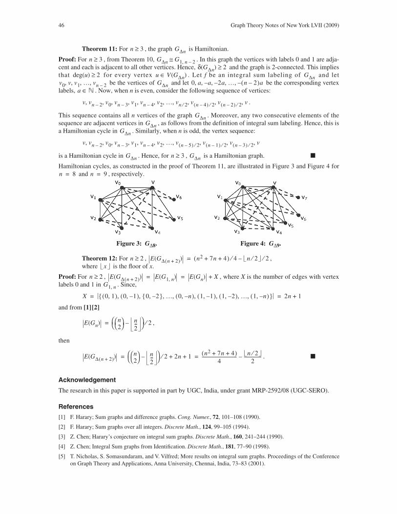
46 Graph Theory Notes of New York LVII (2009)
Theorem 11: For , the graph is Hamiltonian.
Proof: For , from Theorem 10, . In this graph the vertices with labels 0 and 1 are adja-cent and each is adjacent to all other vertices. Hence, and the graph is 2-connected. This impliesthat for every vertex . Let f be an integral sum labeling of and let
be the vertices of and let be the corresponding vertexlabels, . Now, when n is even, consider the following sequence of vertices:
.
This sequence contains all n vertices of the graph . Moreover, any two consecutive elements of thesequence are adjacent vertices in , as follows from the definition of integral sum labeling. Hence, this isa Hamiltonian cycle in . Similarly, when n is odd, the vertex sequence:
is a Hamiltonian cycle in . Hence, for , is a Hamiltonian graph. �
Hamiltonian cycles, as constructed in the proof of Theorem 11, are illustrated in Figure 3 and Figure 4 for and , respectively.
Theorem 12: For , ,where is the floor of x.
Proof: For , , where X is the number of edges with vertexlabels 0 and 1 in . Since,
and from [1][2]
,
then
. �
Acknowledgement
The research in this paper is supported in part by UGC, India, under grant MRP-2592/08 (UGC-SERO).
References
[1] F. Harary; Sum graphs and difference graphs. Cong. Numer., 72, 101–108 (1990).
[2] F. Harary; Sum graphs over all integers. Discrete Math., 124, 99–105 (1994).
[3] Z. Chen; Harary’s conjecture on integral sum graphs. Discrete Math., 160, 241–244 (1990).
[4] Z. Chen; Integral Sum graphs from Identification. Discrete Math., 181, 77–90 (1998).
[5] T. Nicholas, S. Somasundaram, and V. Vilfred; More results on integral sum graphs. Proceedings of the Conferenceon Graph Theory and Applications, Anna University, Chennai, India, 73–83 (2001).
n 3≥ GΔn
n 3≥ GΔn G1 n 2–,≅δ GΔn( ) 2≥
deg u( ) 2≥ u V GΔn( )∈ GΔnv0 v v1 … vn 2–, , , , GΔn 0 a a– 2a– … n 2–( )a–, , , , ,
a �∈
v vn 2– v0 vn 3– v1 vn 4– v2 … vn 2⁄ v n 4–( ) 2⁄ v n 2–( ) 2⁄ v, , , , , , , , , , ,
GΔnGΔn
GΔn
v vn 2– v0 vn 3– v1 vn 4– v2 … v n 5–( ) 2⁄ v n 1–( ) 2⁄ v n 3–( ) 2⁄ v, , , , , , , , , , ,
GΔn n 3≥ GΔn
n 8= n 9=
Figure 3: GΔ8. Figure 4: GΔ9.
n 2≥ E GΔ n 2+( )( ) n2 7n 4+ +( ) 4⁄ n 2⁄ 2⁄–=x
n 2≥ E GΔ n 2+( )( ) E G1 n,( ) E Gn( ) X+= =G1 n,
X 0 1,( ) 0 1–,( ) 0 2–,{ } … 0 n–,( ) 1 1–,( ) 1 2–,( ) … 1 n–,( ), , , , , , , ,{ } 2n 1+= =
E Gn( ) n2⎝ ⎠
⎛ ⎞ n2---–⎝ ⎠
⎛ ⎞ 2⁄=
E GΔ n 2+( )( ) n2⎝ ⎠
⎛ ⎞ n2---–⎝ ⎠
⎛ ⎞ 2⁄ 2n 1+ + n2 7n 4+ +( )4
-------------------------------- n 2⁄2
----------------–= =
K. Vilfred and T. Nicholas: The integral sum graph 47
[6] V. Vilfred; On integral sum graphs. National Seminar on Algebra and Discrete Mathematics, Kerala University,Trivandrum, India (2005).
[7] V. Vilfred and L. Mary Florida; Relation between sum, integer sum, chromatic and edge chromatic numbers of a fewgraphs. (2009) —submitted.
[8] V. Vilfred and L. Mary Florida; Two problems in integral sum labeling. (2009) —submitted.
[9] V. Vilfred and T. Nicholas; Amalgamation of integral sum graphs, fan and dutch m-windmill are integral sum graphs.(2009) —submitted.
[10] V. Vilfred and T. Nicholas; Banana trees and union of stars are integer sum graphs. Ars Combinatoria, (2009) —Accepted for publication.
[11] F. Harary; Graph Theory. Addison Wesley, Reading (1969).
[12] J.A. Gallian; A dynamic survey of graph labeling: 12th Edition. Electronic J. Combinatorics, 16, #DS6 (2009).
Received: October 1, 2007Revised: December 16, 2009

Graph Theory Notes of New York LVII The Mathematical Association of America (2009)
Numerics2-long number, 12
Aadjacency matrix, 39
visibility graph, 17algorithm
A*, 17Dijkstra, 17search, 17
AutoGraphiX, 39
BBacon number, 23brute force method, 27
Ccharacteristic polynomial, 39chromatic number, 39clique
connected cover number, 30covering number, 30number, 39
closed neighborhood, 29conjecture, Locke, 34connected dominating set, 30corona, 31cover, vertex, 29
Ddefending a graph, 29degree matrix, 39deoxyribonucleic acid, 19diagonal degree matrix, 39digraph, overlap, 21Dijkstra algorithm, 17disjoint mirror twin, 34dominating set, 29
connected, 30problem
eternal, 29m-eternal, 29
total, 29domination number, 29dual, Sylvester problem, 15
EErdös
collaboration graph, 23number, 23
eternal dominating set problem, 29even vertex, 34
HHamilton
cycle, 24path, 21, 34
Hamiltonian, 43hypercube, 34
Human Genome Project, 19hypercube, 34
Hamiltonian, 34
Iindependence number, 29independent set, 29induced subgraph, 34integer
k-long, 12oblong, 10
integral sum graph, 43
Jjoint space, 19
KKevin Bacon game, 22k-long integer, 12
LLaplacian matrix
signless, 39spectrum, 39
line, ordinary, 14Locke conjecture, 34
Mmatrix
adjacency, 39diagonal degree, 39signless Laplacian, 39
m-eternaldominating set problem, 29vertex covering problem, 29
mirror twin, 34disjoint, 34
Nnearest neighbor algorithm, 27neighbor vertex, 34neighborhood
closed, 29open, 29
neo-colonization, 30neural network, 18nucleotide, 19number
2-long, 12Bacon, 23chromatic, 39clique, 39clique covering, 30clique-connected cover, 30domination, 29Erdös, 23independence, 29total domination, 29vertex cover, 29
total, 29
Ooblong
graph, 10integer, 10
odd vertex, 34
KEY-WORD INDEX

Graph Theory Notes of New York LVII (2009) 49
open neighborhood, 29
ordinary
line, 14
point, 15
overlap digraph, 21
P
parallel computer architecture, 18
path, Hamilton, 21, 34
Pell equation, 13
planar graph theory, 15
point, ordinary, 15
polynomial, characteristic, 39
problem, 21
eternal dominating set, 29
m-eternal
dominating set, 29
vertex covering, 29
travelling salesperson, 24
projective geometry, 15
pseudoline, 15
Q
question, Sylvester, 14
R
robot technology, 16
S
search algorithm, 17
semi-edge walk, 40
series-parallel graph, 30
shotgun method, 19
signless Laplacian matrix, 39
spectrum, 39
spectrum, signless Laplacian matrix, 39
stem, 31
subgraph, induced, 34
sum graph, 43
integral, 43
Sylvester
problem, dual, 15
question, 14
T
topology, 15
total
dominating set, 29
domination number, 29
vertex cover, 29
number, 29
travelling
salesman problem, 21
salesperson problem, 24
travelling salesman, 21
tree diagram, 24
V
vertex
cover, 29
number, 29
problem, m-eternal, 29
total, 29
even, 34
neighbor, 34
odd, 34
visibility graph, 17
adjacency matrix, 17
W
walk, semi-edge, 40
weighted complete graph, 25

Graph Theory Notes of New York LVII The Mathematical Association of America (2009)
Subscription Request and Address Update Form
Please update/add the following information to the distribution list for future issues of
Graph Theory Notes of New York.
My/library mailing information is as follows:
Individual/Library Name:
Mailing Address:
Attention of (if Library):
Telephone Number:
e-mail address:
Date: Please check if this is an address update: ■
Please check if you are currently a member of the Mathematical Association of America ■
____________________________________________________
RETURN FORM TO: The Editors, Graph Theory Notes of New York:
Graph Theory Notes of New YorkMathematics DepartmentQueens College, CUNYKissena BoulevardFlushing, NY 11367, U.S.A.
For further informatione-mail: [email protected]

Graph Theory Notes of New York LVII The Mathematical Association of America (2009)
Order Form
Printed Copies of Back Issues ofGraph Theory Notes of New York
To obtain printed copies of back issues please use the form below. When ordering clearlyindicate in the table provided the issue(s) and number(s) of copies required. Complete thetotal cost for back issues according to the following fee schedule:
Single copies of issues I through IV $2.00 eachV through IX 3.00 eachX through XIX 4.00 eachXX through LVII 5.00 each
A 10% discount may be applied on orders for 10 issues or more.
Please send:
Back Issues: GTN Issue Number Number of Copies
Total cost for back issues (see schedule above) ______
Donation to MAA Graph Theory Fund ______
Total ______
To: Name:
Mailing Address:
Please make your total payable to the “MAA GRAPH THEORY FUND”and send it to: The Editors
John W. Kennedy and Louis V. QuintasGraph Theory Notes of New YorkMathematics DepartmentQueens College, CUNYKissena BoulevardFlushing, NY 11367, U.S.A.
Thank you.

Graph Theory Notes of New York
Instructions for Contributors
Articles published in Graph Theory Notes of New York are of the following types:
(1) Short contributions, surveys, and research articles in graph theory, related fields, and applications.
(2) Graph theory problems (clean or dirty), partial solutions to problems.
(3) Information about availability of graph theory information such as, preprints and technical reports.
(4) Developments on articles in previous Graph Theory Notes of New York.
Graph Theory Notes of New York is intended to provide for informal exchange of ideas within the graphtheory community. Thus, a good selection of references should be included in each submission.
Please submit contributions to the Editors following the format of a recent issue.
All manuscripts submitted to Graph Theory Notes of New York are refereed. Acceptance is the responsi-bility of the Editors. Accepted articles will not necessarily be published in the order they are received butwith the objective of balancing the content of each issue with respect to diversity of topics and authors.
Preferred articles should be concise, self-contained with respect to definitions, provide adequate back-ground to the subject matter. In general, proofs should be in outline form rather than detailed. Papers con-taining open problems or partial solutions are especially welcome.
Excessive use of figures is discouraged. If used, art work must be submitted in camera ready form (goodquality ink drawings or 1200 dpi laser printer output are acceptable). Text used as items contained in theart work should be in Times Roman and variables used should be italicized. Please note that figures maybe subjected to considerable size reduction and this should be allowed for when preparing the originals.
Electronic submissions are welcome but must be accompanied by a printed copy of the manuscript.
Material from articles published in Graph Theory Notes of New York may be reproduced in publicationselsewhere provided proper acknowledgement is given, for example, by citing the original article.