graphic lambda calculus - wolfram researchgraphic lambda calculus, a visual language that can be...

Graphic Lambda Calculus

Marius Buliga

Institute of Mathematics of the Romanian Academy P.O. Box 1-764, RO 014700Bucharest, [email protected]

Graphic lambda calculus, a visual language that can be used for repre-senting untyped lambda calculus, is introduced and studied. It can alsobe used for computations in emergent algebras or for representing Rei-demeister moves of locally planar tangle diagrams.

1. Introduction

Graphic lambda calculus consists of a class of graphs endowed withmoves between them. It might be considered a visual language in thesense of Erwig [1]. The name comes from the fact that it can be usedfor representing terms and reductions from untyped lambda calculus.Its main move is called the graphic beta move for its relation to thebeta reduction in lambda calculus. However, the graphic beta movecan be applied outside the “sector” of untyped lambda calculus, andthe graphic lambda calculus can be used for other purposes than thatof visually representing lambda calculus.

For other visual, diagrammatic representations of lambda calculussee the VEX language [2], or Keenan’s website [3].

The motivation for introducing graphic lambda calculus comesfrom the study of emergent algebras. In fact, my goal is to eventuallybuild a logic system that can be used for the formalization of certain“computations” in emergent algebras. The system can then be appliedfor a discrete differential calculus that exists for metric spaces with di-lations, comprising Riemannian manifolds and sub-Riemannianspaces with very low regularity.

Emergent algebras are a generalization of quandles; namely, anemergent algebra is a family of idempotent right quasigroups indexedby the elements of an Abelian group, while quandles are self-distribu-tive idempotent right quasigroups. Tangle diagrams decorated byquandles or racks are a well-known tool in knot theory [4, 5].

In Kauffman [6] knot diagrams are used for representing combina-tory logic, thus forming a graphical notation for untyped lambda cal-

Complex Systems, 22 © 2013 Complex Systems Publications, Inc.https://doi.org/10.25088/ComplexSystems.22.4.311

y g g g p ypculus terms. Also, Meredith and Snyder [7] associate to any knot dia-gram a process in pi-calculus.

Is there any common ground between these three apparently sepa-rate fields, namely, differential calculus, logic, and tangle diagrams?As a first attempt for understanding this, I proposed l-scale calculus[8], which is a formalism containing both untyped lambda calculusand emergent algebras. Also, in [9] I proposed a formalism of deco-rated tangle diagrams for emergent algebras and I called “computingwith space” the various manipulations of these diagrams with geomet-ric content. Nevertheless, in that paper I was not able to give a precisesense of the use of the word “computing.” I speculated, by usinganalogies from studies of the visual system, especially the “brain as ageometry engine” paradigm of Koenderink [10], that, in order for thevisual front end of the brain to reconstruct the visual space in thebrain, there should be a kind of “geometrical computation” in theneural network of the brain akin to the manipulation of decorated tan-gle diagrams described in this paper.

I hope to convince the reader that graphic lambda calculus gives arigorous answer to this question, being a formalism that contains, in asense, lambda calculus, emergent algebras, and tangle diagrams.

2. Graphs and Moves

An oriented graph is a pair HV, EL, with V the set of nodes and

E Õ V äV the set of edges. Let us denote by a : V Ø 2E the map thatassociates to any node N œ V the set of adjacent edges aHNL. In thispaper we work with locally planar graphs with decorated nodes; thatis, we shall attach supplementary information to a graph HV, EL.

† A function f : V Ø A that associates to any node N œ V an element ofthe “graphical alphabet” A (see Definition 1).

† A cyclic order of aHNL for any N œ V, which is equivalent to giving a lo-cal embedding of the node N and edges adjacent to it into the plane.

We shall construct a set of locally planar graphs with decoratednodes, starting from a graphical alphabet of elementary graphs. Weshall define local transformations, or moves, on the set of graphs.Global moves or conditions will then be introduced.

Definition 1. The graphical alphabet contains the elementary graphs, orgates, denoted by l, U, !, !, and for any element ! of the commuta-tive group G, a graph denoted by !. Here are the elements of thegraphical alphabet:

312 M. Buliga


l graph , U graph

! graph , ! graph

! graph

With the exception of the ! graph, all other elementary graphs havethree edges. The ! graph has only one edge.

There are two types of “fork” graphs: l and U, and two types of“join” graphs: ! and !. I now briefly explain what they are supposedto represent and why they are needed in this graphic formalism.

The l gate corresponds to the lambda abstraction operation fromuntyped lambda calculus. This gate has one input (the entry arrow)and two outputs (the exit arrows); therefore, at first view, it cannotbe a graphical representation of an operation. In untyped lambda cal-culus the l abstraction operation has two inputs, namely a variablename x and a term A, and one output, the term l x.A. An algorithm ispresented in Section 3 to transform a lambda calculus term into agraph made by elementary gates, such that to any lambda abstractionthat appears in the term there is a corresponding l gate.

The U gate corresponds to a fan-out gate. It is needed because thegraphic lambda calculus described in this paper does not have vari-able names. U gates appear in the process of eliminating variablenames from lambda terms, as described in Section 3.

Another justification for the existence of two fork graphs is thatthey are subjected to different moves: the l gate appears in thegraphic beta move, together with the ! gate, while the U gate appearsin the fan-out moves. Thus, even if the l and U gates have the sametopology, they are subjected to different moves, which in fact charac-terizes their lambda abstraction and fan-out qualities. The alternative,consisting of only one generic fork gate, leads to identifying, in asense, lambda abstraction with fan-out, which would be confusing.

The ! gate corresponds to the application operation from lambdacalculus. The algorithm from Section 3 associates a ! gate to any ap-plication operation used in a lambda calculus term.

Graphic Lambda Calculus 313


The ! gate corresponds to an idempotent right quasigroup opera-tion, which appears in emergent algebras as an abstraction of the geo-metrical operation of taking a dilation (of coefficient !), based at apoint and applied to another point.

The existence of two join gates, with the same topology, is justifiedby the fact that they appear in different moves.

2.1 The Set of GraphsWe now construct the set of graphs graph over the graphical alphabet.

Definition 2. The set of graphs graph is obtained by grafting edges froma finite number of copies of the elements of the graphical alphabet.During the grafting procedure, we start from a set of gates and add afinite number of gates one at a time, such that, at any step, any edgeof any elementary graph is grafted on any other free edge (i.e., not al-ready grafted to another edge) of the graph, with the condition thatthey have the same orientation.

For any node of the graph, the local embedding into the plane isgiven by the element of the graphical alphabet that decorates it.

The set of free edges of a graph G œ graph is named the set ofleaves LHGL. Technically, imagine that we complete the graphG œ graph by adding to the free extremity of any free edge a deco-rated node, called a “leaf,” with decoration “in” or “out,” dependingon the orientation of the respective free edge. The set of leaves LHGLthus decomposes into a disjoint union LHGL ! inHGL ‹ outHGL of in orout leaves.

Moreover, we admit into graph arrows without nodes,

called wires or lines, and loops (without either nodes from the elemen-tary graphs or leaves):

Graphs in graph can be disconnected. Any graph that is a finite re-union of lines, loops, and assemblies of the elementary graphs is ingraph.

2.2 Local MovesThese are transformations of graphs in graph that are local, in thesense that any of the moves apply to a limited part of a graph, keep-ing the rest of the graph unchanged.

314 M. Buliga

Complex Systems, 22 © 2013 Complex Systems Publications, Inc. https://doi.org/10.25088/ComplexSystems.22.4.311

We may define a local move as a rule transforming a graph into an-other of the following form.

First, a subgraph of graph G in graph is any collection of nodesand/or edges of G. It is not supposed that the mentioned subgraphmust be in graph. Also, a collection of some edges of G, without anynode, counts as a subgraph of G. Thus, a subgraph of G might beimagined as a subset of the reunion of nodes and edges of G.

For any natural number N and any graph G in graph, let "HG, NLbe the collection of subgraphs P of the graph G with the sum of thenumber of their edges and nodes less than or equal to N.

Definition 3. A local move has the following form: there is a number Nand a condition C that is formulated in terms of graphs with the sumof the number of their edges and nodes less than or equal to N, suchthat for any graph G in graph and for any P œ "HG, NL, if C is truefor P then transform P into P£, where P£ is also a graph with the sumof the number of its edges and nodes less than or equal to!N.

We may graphically group the elements of the subgraph, subjectedto the application of the local rule, into a region encircled with adashed, closed, simple curve. The edges that cross the curve (thus con-necting the subgraph P with the rest of the graph) will be numberedclockwise. The transformation will affect only the part of the graphthat is inside the dashed curve (inside meaning the bounded connectedpart of the plane that is bounded by the dashed curve) and, after thetransformation is performed, the edges of the transformed graph willconnect to the graph outside the dashed curve by respecting the num-bering of the edges that cross the dashed line.

However, the grouping of the elements of the subgraph has no in-trinsic meaning in graphic lambda calculus. It is just a visual aid andis not a part of the formalism. Sometimes colors are used in the fig-ures as a visual aid. The colors, as well, do not have any intrinsicmeaning in the graphic lambda calculus.

2.2.1 Graphic b Move

This is the most important move, inspired by the b-reduction fromlambda calculus; see Theorem 1, part (d):

The labels “1, 2, 3, 4” are used only as guides for correctly gluingthe new pattern, after removing the old one. As with the encircling



p g g

dashed curve, they have no intrinsic meaning in graphic lambda calcu-lus.

This “sewing braids” move will also be used in contexts outside oflambda calculus! It is the most powerful move in this graphic calcu-lus. A primitive form of this move appears as the rewiring move (W1)[9, pp. 20, 21].

Here is an alternative notation for the sewing braids move:

A move that looks very much like the graphic beta move is the un-zip operation from the formalism of knotted trivalent graphs; see, forexample, [11, Section 3]. In order to see this, we draw the graphicbeta move again, this time without labeling the arrows:

The unzip operation acts only from left to right in the followingfigure. Remarkably, it acts on trivalent graphs (but not oriented):

Let us go back to the graphic beta move and remark that it doesnot depend on the particular embedding in the plane. For example,the intersection of the 1,3 arrow with the 4,2 arrow is an artifact ofthe embedding; there is no node there. Intersections of arrows haveno meaning, since we are working with graphs that are locally planar,not globally planar.

The graphic beta move goes in both directions. In order to applythe move, pick a pair of arrows and label them with 1,2,3,4, suchthat, according to the orientation of the arrows, 1 points to 3 and 4points to 2. There are no nodes or labels between 1 and 3 or between4 and 2. Then, a graphic beta move will replace the portions of thetwo arrows that are between 1 and 3 and between 4 and 2 with thepattern from the left-hand side of the figure, which describes thegraphic beta move.

316 M. Buliga


As an illustration of this, the graphic beta move may be appliedeven to a single arrow or to a loop. The next figure shows three appli-cations of the graphic beta move that illustrate the need to considerloops and wires as members of graph:

We can apply a graphic beta move in different ways to the samegraph and in the same place, simply by using different labels 1, … 4(here A, B, C, D are graphs in graph):

A particular case of the previous figure is yet another justificationfor having loops as elements in graph:



The two previous applications of the graphic beta move may be rep-resented alternatively like this:

2.2.2 Coassociativity Move

This is the coassociativity move involving the U graphs. Consider theU graph as corresponding to a fan-out gate:

318 M. Buliga


By using coassociativity moves, we can move between any two bi-nary trees formed only with U gates, with the same number of outputleaves.

2.2.3 Cocommutativity Move

This is the cocommutativity move involving the U gate. It will be notused until Section 6 concerning knot diagrams:

2.2.3a R1a Move

This move is imported from emergent algebras. Explanations aregiven in Section 5. It involves an U graph and a ! graph, with ! œ G:



2.2.3b R1b Move

Here is the R1b move (also related to emergent algebras):

2.2.4 R2 Move

This corresponds to the Reidemeister II move for emergent algebras.It involves an U graph and two others: a ! and a m graph, with!, m œ G:

The R2 move appears in [9, p. 21], with the supplementary name“triangle move.”

2.2.5 Ext2 Move

This corresponds to the rule (ext2) from l-scale calculus. It expressesthe fact that in emergent algebras the operation indexed with the neu-tral element 1 of the group G has the property x È1 y ! y:

320 M. Buliga


2.2.6 Local Pruning

Local pruning moves are local moves that eliminate dead edges. Notethat, unlike the previous moves, these are one way (you can eliminatedead edges, but not add them to graphs):



2.3 Global Moves or ConditionsGlobal moves are not local either because the condition C applies toparts of the graph that may have an arbitrarily large sum of edgesplus nodes or because after the move the graph P£ that replaces thegraph P has an arbitrarily large sum of edges plus nodes.

2.3.1 Ext1 Move

This corresponds to the rule (ext1) from l-scale calculus, or to h-re-duction in lambda calculus (see Theorem 1, part (e) for details). Itinvolves a l graph (similar to the l abstraction operation in lambdacalculus) and a ! graph (similar to the application operation inlambda calculus).

The rule is: if there is no oriented path from 2 to 1, then the ext1move can be performed:

2.3.2 Global Fan-Out Move

This is a global move that consists of replacing (under certain circum-stances) a graph by two copies of that graph.

The rule is: if a graph in G œ graph has an U bottleneck, that is, if

we can find a subgraph A œ graph connected to the rest of the graphG only through an U gate, then we can perform the move depicted inthe next figure, from the left to the right:

322 M. Buliga


Conversely, if in the graph G we can find two identical subgraphs(denoted by A) that are in graph and have no edge connecting onewith another and that are connected to the rest of G only through oneedge, as in the right-hand side of the figure, then we can perform themove from the right to the left.

Note that global fan-out trivially implies cocommutativity. As a lo-cal rule alternative to the global fan-out, we might consider the follow-ing. Fix a number N and consider only graphs A that have at most N(nodes + arrows). The N local fan-out move is the same as the globalfan-out move, except it only applies to such graphs A. This local fan-out move does not imply cocommutativity.

2.3.3 Global Pruning

This a global move to eliminate dead edges.

The rule is: if a graph in G œ graph has a ! ending, that is, if we

can find a subgraph A œ graph connected only to a ! gate, with noedges connecting to the rest of G, then we can erase this graph andthe respective ! gate:

The global pruning may be needed because of the l gates that can-not be removed only by local pruning.



2.3.4 Elimination of Loops

It is possible that after using a local or global move, we obtain agraph with an arrow that closes itself, without being connected to anynode. For example, if a loop appears after the application of a graphicbeta move, then it can be erased by the elimination of loops move.

2.4 l-graphsThe edges of an elementary graph l can be numbered unambiguously,clockwise, by 1, 2, 3, such that 1 is the number of the entrant edge.

Definition 4. A graph G œ graph is a l-graph, denoted as G œ l graph,if:

† it does not have any ! gates,

† for any node l any oriented path in G starting at edge 2 of this nodecan be completed to a path that either terminates in a graph !, or elseterminates at edge 1 of this node.

The condition G œ l graph is global, in the sense that in order to

decide if G œ l graph, we have to examine parts of the graph thatmay have an arbitrarily large sum of edges plus nodes.

3. Conversion of Lambda Terms

This section describes how to associate a lambda term to a graph ingraph that is then used to show that b-reduction in lambda calculus

transforms into the b rule for graph.Indeed, to any term A œ THXL (where THXL is the set of lambda

terms over the variable set X) we associate its syntactic tree. The syn-tactic tree of any lambda term is constructed by using two gates, onecorresponding to the l abstraction and the other corresponding to theapplication. We draw syntactic trees with the leaves (elements of X)at the bottom and the root at the top. We shall use the following nota-tion for the two gates: at the left is the gate for the l abstraction andat the right is the gate for the application:

Notice that these two gates are from the graphical alphabet ofgraph, but the syntactic tree is decorated: at the bottom we have

324 M. Buliga


leaves from X. Also, notice the peculiar orientation of the edge fromthe left (in tree notation convention) of the l gate. For the moment,this orientation is in contradiction with the implicit orientation (fromdown-up) of edges of the syntactic tree, but soon this matter will be-come clear.

We shall remove all leaf decorations, with the price of introducingnew gates, namely U and !. This will be done in a sequence of steps,detailed later. Take the syntactic tree of A œ THXL, drawn with thementioned conventions (concerning gates and the positioning ofleaves and root, respectively).

We take as examples the following five lambda terms:

I ! lx.xK ! lx.Hly.xLS ! lx.Hly.Hlz.HHxzL HyzLLLLW ! Hlx.HxxLL Hlx.HxxLLT ! Hlx.HxyLL Hlx.HxyLL

3.1 Step 1: List Bound VariablesAny leaf of the tree is connected to the root by a unique path. Startfrom the leftmost leaf, perform the algorithm explained next, then goto the right and repeat until all leaves are exhausted. We also initializea list B ! « of bound variables.

Take a leaf, say decorated with x œ X. To this leaf is associated aword (a list) that is formed by the symbols of gates on the path con-necting (from the bottom up) the leaf with the root, together with in-formation about which way, left (L) or right (R), the path passes

through the gates. Such a word is formed by the letters lL, lR,

!L, !R.

If the first letter is lL, then add to the list B the pair Hx, wHxLLformed by the variable name x and the associated word (describingthe path to follow from the respective leaf to the root). Then pass to anew leaf.

Otherwise, continue along the path to the root. If we arrive at a lgate, which can happen only coming from the right leg of the l gate,

we can find only the letter lR. In such a case look at the variable ythat decorates the left leg of the same l gate. If x ! y, then add a newedge to the syntactic tree from y to x and proceed farther along thepath; otherwise proceed farther. If the root is attained, then pass tothe next leaf.

Here are some examples of graphs associated to the mentionedlambda terms, together with the list of bound variables.



† I ! l x.x has B ! 9Ix, lLM=, K ! lx.Hly.xL has B ! 9Ix, lLM, Iy, lL lRM=, and S ! l x.Hl y.Hl z.HHx zL Hy zLLLL has

B ! 9Ix, lLM, Iy, lL lRM, Iz, lL lR lRM=:

† W ! Hl x.Hx xLL Hl x.Hx xLL has B ! 9Ix, lL !LM, Ix, lL !RM= and

T ! Hl x.Hx yLL Hl x.Hx yLL has B ! 9Ix, lL !LM, Ix, lL !RM=:

3.2 Step 2: Eliminate Bound VariablesWe now have a list B of bound variables. If the list is empty, then goto the next step. Otherwise, do the following, starting from the first el-ement of the list, until the list is finished.

An element, say Hx, wHxLL, of the list is either connected to otherleaves by one or more edges added at step 1 or not. If it is not con-nected, then erase the variable name with the associated path wHxLand replace it with a ! gate. If it is connected, then erase it and re-place it with a tree formed by U gates, starting at the place where theelements of the list were before the erasure and stopping at the leaves

326 M. Buliga


pp g that were connected to x. Erase all decorations that were joined to xand also erase all edges added at step 1 to leaf x from the list.

Here are examples showing the graphs associated to the mentionedlambda terms after step 2.

† The graphs of I ! l x.x, K ! lx.Hly.xL, and S ! l x.Hl y.Hl z.HHx zL Hy zLLLL:

† The graphs of W ! Hl x.Hx xLL Hl x.Hx xLL and T ! Hl x.Hx yLL Hl x.Hx yLL:

Notice that at this step the necessity of having the peculiar orientationof the left leg of the l gate becomes clear.

Note also that there may be more than one possible tree of gates U,for example, at each elimination of a bound variable (in cases when abound variable has at least three occurrences). One may use any treeof U that is fit. The problem of multiple possibilities is the reason forintroducing the coassociativity move.

3.3 Step 3: Remove Leaf DecorationsThere may still be leaves decorated with free variables. Starting fromthe left to the right, group them together in case some of them occurin multiple places, then replace the multiple occurrences of a free vari-able by a tree of U gates with a free root ending exactly at the occur-rences of the respective variables. Again, there are multiple ways of



p g p y doing this, but we may pass from one to another by a sequence ofcoassociativity moves.

Here are examples after step 3. All the graphs associated to thementioned lambda terms, except the last one, are left unchanged. Thegraph of the last term changes.

† The graph of W ! Hl x.Hx xLL Hl x.Hx xLL, left unchanged by step 3, andthe graph of T ! Hl x.Hx yLL Hl x.Hx yLL:

Theorem 1. Let A # @AD be a transformation of a lambda term A into agraph @AD as described previously (multiple transformations are possi-ble because of the choice of U trees). Then:

(a) For any term A the graph @AD is in l graph.

(b) If @AD£ and @AD££ are transformations of the term A, then we may passfrom @AD£ to @AD££ by using a finite number (exponential in the number ofleaves of the syntactic tree of A) of coassociativity moves.

(c) If B is obtained from A by a-conversion, then we may pass from @AD to@BD by a finite sequence of coassociativity moves.

(d) Let A, B œ THXL be two terms and x œ X be a variable. Consider theterms l x.A and A@x := BD, where A@x := BD is the term obtained by sub-stituting in A the free occurrences of x by B. We know that b reductionin lambda calculus consists of passing from Hl x.ALB to A@x := BD. Then,by one b move in graph applied to @Hl x.ALBD we pass to a graph that canbe further transformed into one of A@x := BD, via global fan-out, coasso-ciativity, and pruning moves.

(e) With the notations from (d), consider the terms A and l x.A x withx – FVHAL; then the h reduction, consisting of passing from l x.A x to A,corresponds to the ext1 move applied to the graphs @l x.A xD and @AD.

Proof. (a) We have to prove that, for any node l, any oriented path in@AD starting at the left exiting edge of the l node can be completed as

328 M. Buliga


g g g p

a path that either terminates in a ! graph, or else terminates at theentry peg of the l node, but this is clear. Indeed, either the bound vari-able (of this l node in the syntactic tree of A) is fresh and gets re-placed by a ! gate, or else the bound variable is replaced by a tree ofU gates. No matter which path we choose, we may complete it as acycle passing by the said l node.

(b) Clear also, because the coassociativity move is designed forpassing from a tree of U gates to another tree with the same numberof leaves.

(c) Indeed, the names of bound variables of A do not affect the con-struction of @AD, therefore if B is obtained by a-conversion of A, then@BD differs from @AD only by the particular choice of trees of U gates.But this is solved by coassociativity moves.

(d) This may be the surprising part of the theorem. There are twocases: x is fresh for A or not. If x is fresh for A, then in the graph@Hl x.ALBD the named variable x is replaced by a ! gate. If not, thenall the occurrences of x in A are connected by an U tree with its rootat the left peg of the l gate where x appears as a bound variable.

In the case when x is not fresh for A, the left-hand side of the fig-ure has the graph @Hl x.ALBD (with a remaining decoration of “x”).We perform a graphic b move and obtain the graph on the right:

This graph can be transformed into a graph of A@x := BD via globalfan-out and coassociativity moves. Here is the case when x is freshfor!A:



We see that the graph obtained by performing the graphic b moveis the union of the graph of A and the graph of B with a ! gate addedat the root. After pruning we are left with the graph of A, consistentwith the fact that when x is fresh for A then Hl x.ALB transforms by breduction into A.

(e) In the next figure the left-hand side is the graph @l x.A xD andthe right-hand side is the graph @AD:

The red asterisk marks the arrow that appears in the construction@l x.A xD from the variable x, taking into account the hypothesisx – FVHAL. We have a pattern where we can apply the ext1 move andobtain @AD, as claimed. ·

As an example, let us manipulate the graph of W ! Hl x.Hx xLLHlx.Hx xLL:

330 M. Buliga


We can pass from the left-hand side of the figure to the right-handside by using a graphic b move. Conversely, we can pass from theright-hand side of the figure to the left-hand side by using a global fan-out move. These manipulations correspond to the well-known factthat W remains unchanged after b reduction: let U ! l x.Hx xL, thenW ! U U ! Hl x.Hx xLLU ¨ U U ! W.

3.4 Example: Combinatory LogicThe combinators I ! l x.x, K ! lx.Hly.xL, and S ! l x.Hly.Hlz.

HHx zL Hy zLLLL have the following correspondents in graph, denoted bythe same letters:

Proposition 1. (a) By one graphic b move, I ! A transforms into A, forany A œ graph with one output.

(b) By two graphic b moves followed by a global pruning, for anyA, B œ graph with one output, the graph HK ! AL! B transforms in-to!A.

(c) By five graphic b moves followed by one local pruning move,the graph HS ! KL! K transforms into I.

(d) By three graphic b moves followed by a global fan-out move,for any A, B, C œ graph with one output, the graph HHS ! AL! BL! Ctransforms into the graph HA ! CL! HB ! CL. Proof. The proof of (b) is given as this figure:



The proof of (c) is given as this figure:

(a) and (d) are left to the interested reader. ·

4. Using Graphic Lambda Calculus

The graph manipulations presented in this section can be applied forgraphs that represent lambda terms. However, they can also be ap-plied for graphs that do not represent lambda terms.

4.1 Fixed PointsLet us start with a graph A œ graph that has one distinguished inputand one distinguished output represented as follows:

332 M. Buliga


For any graph B with one output, we denote by AHBL the graph ob-tained by grafting the output of B to the input of A.

I want to find B such that AHBL ¨ B, where ¨ means any finite se-quence of moves in graphic lambda calculus. Such a graph B is calleda fixed point of A.

The solution of this problem is the same as in usual lambda calcu-lus. We start from the following succession of moves:

This is very close to the solution; we only need a small modifica-tion:



4.2 Grafting: Application or Abstraction?If the A, B from the previous paragraph represent lambda terms, thenthe natural operation between them is not grafting, but the applica-tion. Or, in graphic lambda calculus the application is represented byan elementary graph, therefore A B (seen as the term in lambda cal-culus obtained as the application of A to B) is not represented as agrafting of the output of B to the input of A.

We can easily transform grafting into the application operation:

Suppose that A and B are graphs representing lambda terms. Moreprecisely, suppose that A is representing a term (also denoted by A)and its input represents a free variable x of the term A. Then, thegrafting of B to A is the term A@x := BD and the graph from the rightis representing Hl x.ALB; therefore, both graphs are representing termsfrom lambda calculus.

334 M. Buliga


We can transform grafting into something else:

This has no meaning in lambda calculus, but it looks as if the ab-straction gate (the l gate) plays the role of an application operation,except for the orientation of one of the arrows of the graph from theright.

4.3 Zippers and Combinators as Half-ZippersLet us take n ¥ 1 to be a natural number and let us consider the fol-lowing graph in graph, called the n-zipper:

At the left is the n-zipper graph; at the right is a notation for it, or a“macro.” The zipper graph is interesting because it allows performing(nontrivial) graphic beta moves in a fixed order. In the following fig-ure, red depicts the place where the first graphic beta move is applied:



This graphic beta move has the following appearance in zippernotation:

We see that an n-zipper transforms into an Hn-1L-zipper plus an ar-row. This move may be repeated as long as possible. This proceduredefines a zipper move:

We may consider the 1-zipper move the same as the graphic betamove, transforming the 1-zipper into two arrows.

336 M. Buliga


The combinator I ! l x.x satisfies the relation I A ! A. The nextfigure shows that I (in green), when applied to A, is just a half of the1-zipper, with an arrow added (in blue):

By opening the zipper we obtain A, as we should. The combinator K ! l x y.x satisfies K A B ! HK ALB ! A. In the

next figure the combinator K (in green) appears as half of the 2-zip-per, with one arrow and one termination gate added (in blue):

After opening the zipper we obtain a pair made by A and B that getsthe termination gate on top of it. A global pruning move sends B tothe trash bin.

Finally, the combinator S ! l x y z.HHx zL Hy zLL satisfiesS A B C ! HHS ALBLC ! HA CL HB CL. The combinator S (in green) ap-pears to be made by half of the 3-zipper, with some arrows and alsowith a “diamond” added (all in blue). Interestingly, the diamondlooks similar to the ones from Definition 8 in Section 5.



Expressed with the help of zippers, the relation S K K ! I appearslike this:

338 M. Buliga


4.4 Lists and CurryingWith the help of zippers, we may enhance the procedure of turninggrafting into the application operation. We have a graph A œ graphthat has one output and several inputs:



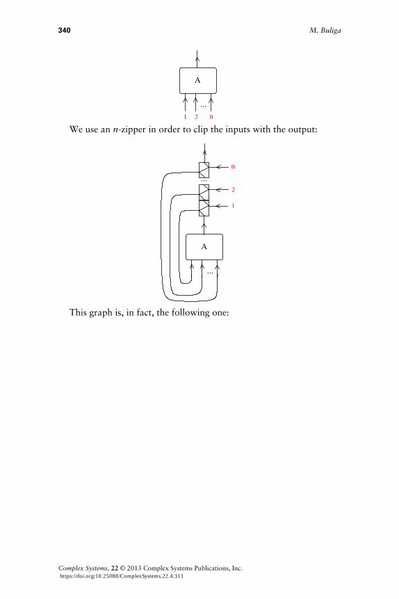
We use an n-zipper in order to clip the inputs with the output:

This graph is, in fact, the following one:

340 M. Buliga


We may interpret the graph inside the green dotted rectangle as thecurrying of A, called curryHAL. This graph has only one output and noinputs. The graph inside the red dotted rectangle is almost a list. Weshall transform it into a list by again using a zipper and one graphicbeta move:



4.5 Packing ArrowsWe may pack several arrows into one. The case of two arrows is de-scribed first. We start from the following sequence of three graphicbeta moves:

342 M. Buliga


This figure means: we pack the 1,2 entries into a list, pass it throughone arrow, then unpack the list into the outputs 3,4. Of course, thispacking/unpacking trick may be used for more than a pair of arrows,in obvious ways; therefore, it is not a restriction of generality to writeonly about two arrows.

We may apply the trick to a pair of graphs A and B that are con-nected by a pair of arrows, as in the following figure:

With the added packing/unpacking triples of gates, the graphs A, Bare interacting only by the intermediary of one arrow.

In particular, we may use this trick for the elementary gates of ab-straction and application, transforming them into graphs with one in-put and one output, like this:

If we use the elementary gates transformed into graphs with oneinput and one output, the graphic beta move becomes this almost-algebraic, one-dimensional rule:



With such procedures, we may transform any graph in graph into aone-dimensional string of graphs, consisting of transformed elemen-tary graphs and packers/unpackers of arrows, which could be used, inprinciple, for transforming graphic lambda calculus into a text pro-gramming language.

5. Emergent Algebras

Emergent algebras [12, 13] are a distillation of differential calculus inmetric spaces with dilations [14]. This class of metric spaces containsthe “classical” Riemannian manifolds, as well as fractal-like spacessuch as Carnot groups or, more generally, sub-Riemannian or Carnot–Carathéodory spaces (see Bellaïche [15] or Gromov [16]), endowedwith an intrinsic differential calculus based on some variant of thePansu derivative [17].

In [14, Section 4] I proposed a formalism for making various calcu-lations easier with dilation structures. This formalism works withmoves acting on binary decorated trees, with the leaves decoratedwith elements of a metric space.

Here is an example of the formalism. The moves are (with thesame names as those used in graphic lambda calculus; see the explana-tion below):

344 M. Buliga


Define the following graph (consider it as the graphical representa-tion of an operation u + v with respect to the basepoint!x):

Then, in the binary trees formalism the following “approximate”associativity relation can be proved, by using the moves R1a, R2a (itis approximate because a basepoint appears that is different from x,but is close to x in the geometric context of spaces with dilations):

It was puzzling that the formalism worked without needing toknow which metric space is used. Moreover, reasoning with movesacting on binary trees gave proofs of generalizations of results fromsub-Riemannian geometry, while classical proofs involve elaborate cal-culations with pseudo-differential operators. At a close inspection itlooked like somewhere in the background there is an abstract non-sense machine that is applied just to the particular case of sub-Rieman-nian spaces.



In this paper I shall take the following pure algebraic definition ofan emergent algebra (compare with [12, Definition 5.1]), which is astronger version of [13, Definition 4.2] of a G idempotent right quasi-group, in the sense that I define a G idempotent quasigroup here.

Definition 5. Let G be a commutative group with neutral elements de-noted by 1 and operation denoted multiplicatively. A G idempotentquasigroup is a set X endowed with a family of operationsÈ! : XäX Ø X, indexed by ! œ G, such that:

1. For any ! œ G\81< the pair HX, È!L is an idempotent quasigroup; that is,for any a, b œ X the equations x È! a ! b and a È! x ! b have uniquesolutions, and moreover x È! x ! x for any x œ X.

2. The operation È1 is trivial: for any x, y œ X we have x È1 y ! y.

3. For any x, y œ X and any !, m œ G we have: x È! Ix Èm yM ! x È!m y.

Here are some examples of G idempotent quasigroups.

Example 1. Real (or complex) vector spaces: let X be a real (complex)vector space, G ! H0, +¶L (or G ! C*), with multiplication as the op-eration. We define for any ! œ G the following quasigroup operation:x È! y ! H1 - !L x + ! y. These operations give to X the structure of a Gidempotent quasigroup. Note that x È! y is the dilation, based at x, ofcoefficient !, applied to y.

Example 2. Contractible groups: let G be a group endowed with agroup morphism f : G Ø G. Let G ! ! with the operation of integeraddition (thus we may adapt Definition 5 to this example by using“! + m” instead of “!m” and “0” instead of “1” as the name of the

neutral element of G). For any ! œ ! let x È! y ! x f! Ix-1 yM. This is a! idempotent quasigroup. The most interesting case is the one when fis a uniformly contractive automorphism of a topological group G.The structure of these groups is an active exploration area; see, for ex-ample, [18] and the bibliography therein. A fundamental result here isSiebert [19], which gives a characterization of topologically con-nected, contractive, locally compact groups as being nilpotent Liegroups endowed with a one-parameter family of dilations, that is, al-most Carnot groups.

Example 3. A group with an invertible self-mapping f : G Ø G suchthat fHeL ! e, where e is the identity of the group G. It looks likeExample 2 but shows that there is no need for f to be a group mor-phism.

5.1 Local VersionsWe may accept that there is a way (definitely needing a careful formu-lation, but intuitively clear) to define a local version of the notion of a

346 M. Buliga


y

G idempotent quasigroup. With such a definition, for example, a con-vex subset of a real vector space gives a local H0, +¶L idempotentquasigroup (as in Example 1) and a neighborhood of the identity of atopological group G. An identity-preserving, locally-defined, invert-ible self map (as in Example 3) gives a ! local idempotent quasigroup.

Example 4. A particular case of Example 3 is a Lie group G with the op-

erations defined for any ! œ H0, +¶L by x È! y ! x exp I! log Ix-1 yMM. Example 5. A less-symmetric example is the one of X’s being a Rieman-nian manifold, with associated operations defined for any ! œ H0, +¶Lby x È! y ! expxI! logxHyLM, where exp is the metric exponential.

Example 6. More generally, any metric space with dilations is a localidempotent (right) quasigroup.

Example 7. One-parameter deformations of quandles. A quandle is aself-distributive quasigroup. Now, take a one-parameter family ofquandles (indexed by ! œ G) that also satisfies points 2 and 3 fromDefinition 5. What is interesting about this example is that quandlesappear as decorations of knot diagrams [4, 5], which are preserved bythe Reidemeister moves (more on this in Section 6). At closer examina-tion, Examples 1 and 2 are particular cases of one-parameter quandledeformations!

The operations of approximate sum and approximate difference as-sociated to a G idempotent quasigroup are defined next.

Definition 6. For any ! œ G we give the following names to several com-binations of operations of emergent algebras:

† The approximate sum operation is S!x Hu, vL ! x •! HHx È! uL È! vL.

† The approximate difference operation is D!x Hu, vL ! Hx È! uL •! Hx È! vL.

† The approximate inverse operation is inv!x u ! Hx È! uL •! x.

Here is the approximate sum operation for Example 1:

‚!

x Hu, vL ! uH1 - !L - x + v.

It is clear that, as ! converges to 0, this becomes the operation of addi-tion in the vector space with x as a neutral element. It might be saidthat it is the operation of addition of vectors in the tangent space at x,where x is seen as an element of the affine space constructed over thevector space from Example 1.

This is a general phenomenon that becomes really interesting innoncommutative situations, as in the examples from the end of theprovided list.



These approximate operations have many algebraic properties thatcan be found by the abstract nonsense of manipulating binary trees.

Another construction that can be done in emergent algebras is tak-ing finite differences (at a high level of generality, not bound to vectorspaces).

Definition 7. Let A : X Ø X be a function (from X to itself, for simplic-ity). Here is the finite difference function associated to A, with respectto the emergent algebra over X, at a point x œ X:

T!x A : X Ø X , T!

x AHuL ! A HxL •! HA Hx È! uLL.For Example 1, the finite difference has the expression:

T!x A Hu - xL ! A HxL + 1

!HA Hx + ! uL - AHxLL,

which is a finite difference indeed. In more generality, for Example 2this definition leads to the Pansu derivative [17].

Finite differences as defined here behave like discrete versions ofderivatives. Again, the proofs consist of manipulating well-chosen bi-nary trees.

All this can be formalized in graphic lambda calculus, thus trans-forming the proofs into computations inside graphic lambda calculus.

I shall not stress this further, with the exception of describing theemergent algebra sector of graphic lambda calculus.

Definition 8. For any ! œ G, the following graphs in graph areintroduced.

† The approximate sum graph S!:

348 M. Buliga


† The approximate difference graph D!:

† The approximate inverse graph inv!:

Let A be a set of symbols a, b, c, … (these symbols will play therole of scale parameters going to 0). With A and with the Abelian

group G we construct a larger Abelian group G that is generated by Aand by G.

Now we introduce the emergent algebra sector (over the set A).

Definition 9. The subset of graph emerHAL (over the group G) is gener-ated by the following list of gates.

† Arrows and loops.

† The U and ! gates for any ! œ G.

† The approximate sum gate Sa and the approximate difference gate Da,for any a œ A.

The operations of linking output to input arrows need the followinglist of moves.

† Fan-out moves.

† Emergent algebra moves for the group G.

† Pruning moves.

The set emerHAL with the given list of moves is called the emergent al-gebra sector over the set A.



The approximate inverse is not included in the list of generatinggates because we can easily prove that for any a œ A we haveinva œ emerHAL. (If ! œ G then we trivially have inv! œ emerHAL be-cause it is constructed from emergent algebra gates decorated by ele-ments in G that are in the list of generating gates.) Here is the proof:we start with the approximate difference Da and an U gate. We arriveat the approximate inverse inva by the following sequence of moves:

We proved the following relation for emergent algebras:Da

x Hu, xL ! invax u. This relation appears as a computation in graphic

lambda calculus. For the finite differences, we proceed as in Definition 10.

Definition 10. A graph A œ graph, with one input and one output distin-

guished, is computable with respect to the group G if the followinggraph

350 M. Buliga


can be transformed by the moves from graphic lambda calculus into agraph made by assembling:

† graphs from emerHAL† gates l, !, and !

It would be interesting to mix the emergent algebra sector with thelambda calculus sector (in a sense this is already suggested in Defini-tion 10). At first view, it seems that the emergent algebra ! gates areoperations that are added to the lambda calculus operations, the lat-ter being more basic than the former. I think this is not the case. Inthe formalism of lambda-scale calculus [8, Theorem 3.4] (of whichgraphic lambda calculus is a visual variant), I show to the contrarythat emergent algebra gates could be applied to lambda terms and theresult would be a collection, or hierarchy, of lambda calculi, orga-nized into an emergent algebra structure. This is surprising, at leastfor the author, because the initial goal of introducing lambda-scalecalculus was to mimic lambda calculus with emergent algebraoperations.

6. Crossings

In this section we discuss tangle diagrams and graphic lambdacalculus.

An oriented tangle is a collection of wires in three-dimensionalspace; more precisely it is an embedding of an oriented one-dimen-sional manifold in three-dimensional space. Two tangles are the sameup to topological deformation of the three-dimensional space. An ori-ented tangle diagram is, visually, a projection of a tangle, in generalposition, on a plane. More specifically, an oriented tangle diagram isa globally planar oriented graph with 4-valent nodes representingcrossings of wires (as seen in the projection), along with supplemen-tary information about which wire passes over the respective crossing.A locally planar tangle diagram is an oriented graph that satisfies theprevious description, with the exception that it is only locally planar.Visually, a locally planar tangle diagram looks like an ordinary one,except that there may be crossings of edges of the graph that are nottangle crossings (i.e., nodes of the graph).

The purpose of this section is to show that we can “simulate” tan-gle diagrams with graphic lambda calculus. This can be expressedmore precisely in two ways. The first way is to define “crossingmacros,” which are certain graphs that play the role of crossings in atangle diagram (i.e., we can express the Reidemeister moves, de-scribed later, as compositions of moves from graphic lambda calculus



p g p

between such graphs). The second way is to associate a graph ingraph to any tangle diagram such that a certain composition of movesfrom graphic lambda calculus is associated to any Reidemeister move.

Meredith and Snyder [7] achieve this goal using pi-calculus insteadof graphic lambda calculus. Kauffman, in the second part of [6], asso-ciates tangle diagrams to combinators and writes about “knotlogic.”

6.1 Oriented Reidemeister MovesTwo tangles are the same, up to topological equivalence, if and only ifany tangle diagram of one tangle can be transformed by a finite se-quence of Reidemeister moves into a tangle diagram of the second tan-gle. Here are the oriented Reidemeister moves (using the same namesas Polyak [20], but with the letter W replaced by the letter!R).

† Four oriented Reidemeister moves of type 1:

† Four oriented Reidemeister moves of type 2:

352 M. Buliga


† Eight oriented Reidemeister moves of type 3:

6.2 Crossings from Emergent AlgebrasSection 5, Example 7 mentions that there is a connection between tan-gle diagrams and emergent algebras, via the notion of a quandle.Quandles are self-distributive idempotent quasigroups that were in-vented as decorations for the arrows of a tangle diagram, which are in-variant with respect to the Reidemeister moves.

Here are the emergent algebra crossing macros:

We can choose to neglect the ! decorations of the crossings, or, onthe contrary, we can do as in Definition 9 and add a set A to thegroup G and use even more nuanced decorations for the crossings.



In [9, Sections 3 through 6] the use of these crossings for exploringemergent algebras and spaces with dilations is presented. All construc-tions and reasonings from there can be put into the graphic lambdacalculus formalism. Here I shall explain only some introductory facts.

Let us associate to any locally planar tangle diagram T a graph in@TD œ graph, called the translation of T, which is obtained by replac-ing the crossings with the emergent crossing macros (for a fixed !).Also, to any Reidemeister move we associate its translation in graphiclambda calculus, consisting of a local move between the translationsof the left- and right-hand side tangles that appear in the respectivemove. (Note: these translations are not added to the moves that de-fine graphic lambda calculus.)

Theorem 2. The translations of all oriented Reidemeister moves oftypes 1 and 2 can be realized as sequences of the following movesfrom graphic lambda calculus: emergent algebra (i.e., R1a, R1b, R2,ext2), fan-out (i.e., cocommutativity, coassociativity, global fan-out),and pruning. More precisely, the translations of the Reidemeistermoves R1a, R1b are, respectively, the graphic lambda calculus movesR1a, R1b, modulo fan-out moves. Moreover, all translations of Reide-meister moves of type 2 can be expressed in graphic lambda calculuswith the R2, fan-out, and pruning moves.

The proof is left to the interested reader; see however [9, Sec-tion!3.4].

The fact that Reidemeister moves of type 3 are not true for (thealgebraic version of) the emergent algebras, that is, that the transla-tions of the type 3 moves cannot be expressed as a sequence of movesfrom graphic lambda calculus, is a feature of the formalism and not aweakness. This is explained in detail in [9, Sections 5 and 6], but un-fortunately at the moment of writing that paper, the graphic lambdacalculus was not available. It would be interesting to express the con-structions from the mentioned sections in [9] as statements aboutcomputability in the sense of Definition 10 with translations of cer-tain tangle diagrams.

As a justification for this point of view, let us remark that all tanglediagrams that appear in the Reidemeister moves of type 3 have trans-lations that are related to the approximate difference or approximatesum graphs from Definition 8. For example, let us take the translationof the graph from the right-hand side of the move R3d and call it D.This graph has three inputs and three outputs. Let us then consider agraph formed by grafting three graphs A, B, and C at the inputs of D,such that A, B, and C are not otherwise connected. Then we can per-form the following sequence of moves:

354 M. Buliga


The lower-left graph is formed by an approximate difference, a ! gate,and several U gates. Therefore, if A, B, and C are computable in thesense of Definition 8, then the initial graph (the translation of the left-hand side of R3d with A, B, and C grafted at the inputs) is alsocomputable.

6.3 Graphic Beta Move as BraidingWe now construct crossings, in the sense previously explained, usinggates from lambda calculus:

As previously, we define translations of (locally planar) tangle dia-grams into graphs in graph. There is a one-to-one correspondence be-tween the class of locally planar tangle diagrams and a class of graphsin graph. We call this the l-tangle class.

We could proceed in the inverse direction; namely, consider theclass of l-tangle graphs, along with graphic beta moves and elimina-



g g p g g p

tion of loops. Then, we make the (inverse) translation of graphs inl-tangle into locally planar tangle diagrams and the (inverse) transla-tion of the graphic beta move and the elimination of loops. Proposi-tion 2 explains what we obtain.

Proposition 2. The class of l-tangle graphs is closed with respect to theapplication of the graphic beta move and elimination of loops. Thetranslations of the graphic beta and elimination of loops moves arethe Splice 1, 2 (translation of the graphic beta move) and Loop 1, 2(translation of the elimination of loops) moves:

Proof. The proposition becomes obvious if we find the translation ofthe graphic beta move. There is one translation for each crossing:

356 M. Buliga


Likewise, there are two translations for the elimination of loops, de-pending on the orientation of the loop that is added/erased. ·

Theorem 3 clarifies which oriented Reidemeister moves can be ex-pressed as sequences of graphic lambda calculus moves applied tographs in a l-tangle. Among these moves, some are more powerfulthan others, as witnessed by the following.

Theorem 3. All the translations of an oriented Reidemeister move intomoves between graphs in a l-tangle, except R2c, R2d, R3a, and R3h,can be realized as sequences of graphic beta and elimination of loopsmoves. Moreover, the translations of moves R2c, R2d, R3a, and R3hare equivalent up to graphic beta and elimination of loops moves (i.e.,any of these moves, together with graphic beta and elimination ofloops, generate the other moves in this list).

Proof. It is easy, but tedious, to verify that all the mentioned movescan be realized as sequences of splice and loop moves. It is easy to ver-ify that the moves R2c, R2d, R3a, and R3h are equivalent up to spliceand loop moves. It is not obvious that the moves R2c, R2d, R3a, andR3h cannot be realized as a sequence of splice and loop moves. In or-



q p p

der to do this, we prove that R2d cannot be generated by splice andloop. Thanks are due to Peter Kravchuk for the idea of the proof,given in an answer to a question I asked on mathoverflow [21], whereI described the moves splice and loop.

To any locally planar tangle diagram A associate its reduced dia-gram RHAL, which is obtained by the following procedure: first usesplice 1,2 from left to right for all crossings, then use loop 1,2 fromright to left in order to eliminate all loops present at this stage. Notethe following.

† The order of applying splice moves does not matter, because they areapplied only once per crossing. There is a finite number of splices,equal to the number of crossings. Define the bag of splices spliceHAL tobe the set of splice moves applied.

† The same is true for the order of loop elimination by loop 1,2. There isa finite number of loop eliminations, because the number of loops (atthis stage) cannot be bigger than the number of edges of the initial dia-gram. Define the bag of loops loopHAL to be the set of all loops presentafter all splices are done.

Let us now check that the reduced diagram does not change if oneof the four moves is applied to the initial diagram.

Apply a splice 1,2 move to the initial diagram A, from left to right,and get B. Then spliceHBL is what is left in the bag spliceHAL after tak-

ing out the respective splice. Also, loopHBL ! loopHAL because of thedefinition of bags of loops. Therefore, RHAL ! RHBL.

Apply a splice 1,2 from right to left to A and get B. Then,RHAL ! RHBL by the same proof, with A, B switching places.

Apply a loop 1,2 move from left to right to A and get B. The newloop introduced in the diagram does not participate in any crossing(therefore, spliceHAL ! spliceHBL), so we find it in the bag of loops of B

made by all the elements of loopHAL and this new loop. Therefore,RHAL ! RHBL. The same goes for loop 1,2 applied from right to left.

Finally, the reduced diagram of the left-hand side of the move R2dis different from the reduced diagram of the right-hand side of themove R2d; therefore, the move R2d cannot be achieved with a se-quence of splices and loop addition/elimination. ·

Acknowledgments

This work was supported by a grant of the Romanian NationalAuthority for Scientific Research, CNCS UEFISCDI, project numberPN-II-ID-PCE-2011-3-0383.

358 M. Buliga


References

[1] M. Erwig, “Abstract Syntax and Semantics of Visual Languages,” Jour-nal of Visual Languages and Computing, 9(5), 1998 pp. 461–483.doi:10.1006/jvlc.1998.0098.

[2] W. Citrin, R. Hall, and B. Zorn, “Programming with Visual Expres-sions,” Proceedings of the 11th IEEE Symposium on Visual Languages,Darmstadt, 1995 pp. 294–301. doi:10.1109/VL.1995.520822.

[3] D. C. Keenan. “To Dissect a Mockingbird: A Graphical Notation forthe Lambda Calculus with Animated Reduction.” (Oct 2, 2013)http://dkeenan.com/Lambda.

[4] R. Fenn and C. Rourke, “Racks and Links in Codimension Two,” Jour-nal of Knot Theory and its Ramifications, 1(4), 1992 pp. 343–406.

[5] D. Joyce, “A Classifying Invariant of Knots; the Knot Quandle,” Jour-nal of Pure and Applied Algebra, 23(1), 1982 pp. 37–65.doi:10.1016/0022-4049(82)90077-9.

[6] L. Kauffman (ed.), Knot Logic: Knots and Applications (Series on Knotsand Everything, Vol. 6), River Edge, NJ: World Scientific, 1995.

[7] L. G. Meredith and D. F. Snyder, “Knots as Processes: A New Kind ofInvariant.” http://arxiv.org/abs/1009.2107.

[8] M. Buliga, “l-Scale, a Lambda Calculus for Spaces with Dilations.”http://arxiv.org/abs/1205.0139.

[9] M. Buliga, “Computing with Space: A Tangle Formalism for Chora andDifference.” http://arxiv.org/abs/1103.6007.

[10] J. J. Koenderink, “The Brain a Geometry Engine,” Psychological Re-search, 52(2–3), 1990 pp. 122–127.

[11] D. P. Thurston, “The Algebra of Knotted Trivalent Graphs and Tu-raev’s Shadow World.” http://arxiv.org/abs/math/0311458.

[12] M. Buliga, “Emergent Algebras.” http://arxiv.org/abs/0907.1520.

[13] M. Buliga, “Braided Spaces with Dilations and sub-Riemannian Symmet-ric Spaces,” in Geometry. Exploratory Workshop on Differential Ge-ometry and its Applications (D. Andrica and S. Moroianu, eds.),Cluj-Napoca, Romania: Cluj University Press, 2011 pp. 21–35.http://arxiv.org/abs/1005.5031.

[14] M. Buliga, “Dilatation Structures I. Fundamentals,” Journal of General-ized Lie Theory and Applications, 1(2), 2007 pp. 65–95.http://arxiv.org/abs/math/0608536.

[15] A. Bellaïche, “The Tangent Space in sub-Riemannian Geometry,” in Sub-Riemannian Geometry (A. Bellaïche and J.-J. Risler, eds.), Progress inMathematics, 144, Boston: Birkhäuser, 1996 pp. 4–78.

[16] M. Gromov, “Carnot-Carathéodory Spaces Seen from Within,” in Sub-Riemannian Geometry (A. Bellaïche and J.-J. Risler, eds.), Progress inMathematics, 144, Boston: Birkhäuser, 1996 pp. 79–323.



[17] P. Pansu, “Métriques de Carnot-Carathéodory et quasi-isométries des es-paces symétriques de rang un,” Annals of Mathematics, 129(2), 1989pp. 1–60.

[18] H. Glöckner, “Contractible Lie Groups over Local Fields,” Mathema-tische Zeitschrift, 260(4), 2008 pp. 889–904.doi:10.1007/s00209-008-0305-x.

[19] E. Siebert, “Contractive Automorphisms on Locally Compact Groups,”Mathematische Zeitschrift, 191(1), 1986 pp. 73–90.doi:10.1007/BF01163611.

[20] M. Polyak, “Minimal Generating Sets of Reidemeister Moves.”http://arxiv.org/abs/0908.3127.

[21] M. Buliga. “Oriented Reidemeister Move R2d by Splices and LoopAdding/Erasing?” MathOverflow. (Oct 2, 2013)mathoverflow.net/questions/128511.

360 M. Buliga


graphic lambda calculus - wolfram researchgraphic lambda calculus, a visual language that can be...

Documents