Graphical Modeling and Animation of Brittle Fracture

James F. O’Brien Jessica K. Hodgins

GVU Center and College of ComputingGeorgia Institute of Technology

Abstract

In this paper, we augment existing techniques for simulating flex-ible objects to include models for crack initiation and propagationin three-dimensional volumes. By analyzing the stress tensors com-puted over a finite element model, the simulation determines wherecracks should initiate and in what directions they should propagate.We demonstrate our results with animations of breaking bowls,cracking walls, and objects that fracture when they collide. Byvarying the shape of the objects, the material properties, and theinitial conditions of the simulations, we can create strikingly dif-ferent effects ranging from a wall that shatters when it is hit by awrecking ball to a bowl that breaks in two when it is dropped onedge.

CR Categories: I.3.5 [Computer Graphics]: ComputationalGeometry and Object Modeling—Physically based modeling;I.3.7 [Computer Graphics]: Three-Dimensional Graphics andRealism—Animation; I.6.8 [Simulation and Modeling]: Types ofSimulation—Animation

Keywords: Animation techniques, physically based modeling,simulation, dynamics, fracture, cracking, deformation, finite ele-ment method.

1 Introduction

With the introduction in 1998 of simulated water inAntz [5, 14]and clothing inGeri’s Game[4, 15], passive simulation was clearlydemonstrated to be a viable technique for commercial animation.The appeal of using simulation for objects without an internalsource of energy is not surprising, as passive objects tend to havemany degrees of freedom, making keyframing or motion capturedifficult. Furthermore, while passive objects are often essential tothe plot of an animation and to the appearance or mood of the piece,they are not characters with their concomitant requirements for con-trol over the subtle details of the motion. Therefore, simulations inwhich the motion is controlled only by initial conditions, physicalequations, and material parameters are often sufficient to produceappealing animations of passive objects.

College of Computing, Georgia Institute of Technology, Atlanta, GA 30332.job@acm.org, jkh@cc.gatech.edu.

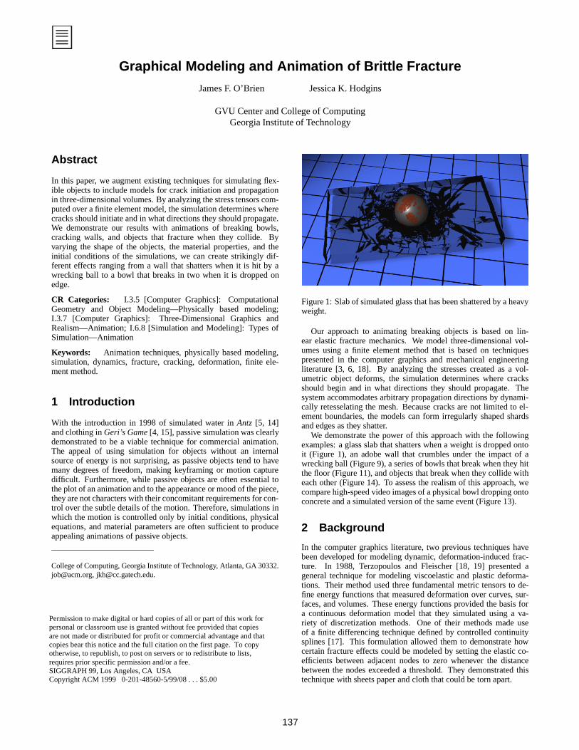
Figure 1: Slab of simulated glass that has been shattered by a heavyweight.

Our approach to animating breaking objects is based on lin-ear elastic fracture mechanics. We model three-dimensional vol-umes using a finite element method that is based on techniquespresented in the computer graphics and mechanical engineeringliterature [3, 6, 18]. By analyzing the stresses created as a vol-umetric object deforms, the simulation determines where cracksshould begin and in what directions they should propagate. Thesystem accommodates arbitrary propagation directions by dynami-cally retesselating the mesh. Because cracks are not limited to el-ement boundaries, the models can form irregularly shaped shardsand edges as they shatter.

We demonstrate the power of this approach with the followingexamples: a glass slab that shatters when a weight is dropped ontoit (Figure 1), an adobe wall that crumbles under the impact of awrecking ball (Figure 9), a series of bowls that break when they hitthe floor (Figure 11), and objects that break when they collide witheach other (Figure 14). To assess the realism of this approach, wecompare high-speed video images of a physical bowl dropping ontoconcrete and a simulated version of the same event (Figure 13).

2 Background

In the computer graphics literature, two previous techniques havebeen developed for modeling dynamic, deformation-induced frac-ture. In 1988, Terzopoulos and Fleischer [18, 19] presented ageneral technique for modeling viscoelastic and plastic deforma-tions. Their method used three fundamental metric tensors to de-fine energy functions that measured deformation over curves, sur-faces, and volumes. These energy functions provided the basis fora continuous deformation model that they simulated using a va-riety of discretization methods. One of their methods made useof a finite differencing technique defined by controlled continuitysplines [17]. This formulation allowed them to demonstrate howcertain fracture effects could be modeled by setting the elastic co-efficients between adjacent nodes to zero whenever the distancebetween the nodes exceeded a threshold. They demonstrated thistechnique with sheets paper and cloth that could be torn apart.

Permission to make digital or hard copies of all or part of this work forpersonal or classroom use is granted without fee provided that copiesare not made or distributed for profit or commercial advantage and thatcopies bear this notice and the full citation on the first page. To copyotherwise, to republish, to post on servers or to redistribute to lists,requires prior specific permission and/or a fee.SIGGRAPH 99, Los Angeles, CA USACopyright ACM 1999 0-201-48560-5/99/08 . . . $5.00

137

In 1991, Norton and his colleagues presented a technique foranimating 3D solid objects that broke when subjected to largestrains [12]. They simulated a teapot that shattered when droppedonto a table. Their technique used a spring and mass system tomodel the behavior of the object. When the distance betweentwo attached mass points exceeded a threshold, the simulation sev-ered the spring connection between them. To avoid having flexi-ble strings of partially connected material hanging from the object,their simulation broke an entire cube of springs at once.

Two limitations are inherent in both of these methods. First,when the material fails, the exact location and orientation of thefracture are not known. Rather the failure is defined as the entireconnection between two nodes, and the orientation of the fractureplane is left undefined. As a result, these techniques can only re-alistically model effects that occur on a scale much larger than theinter-node spacing.

The second limitation is that fracture surfaces are restricted to theboundaries in the initial mesh structure. As a result, the fracture pat-tern exhibits directional artifacts, similar to the “jaggies” that occurwhen rasterizing a polygonal edge. These artifacts are particularlynoticeable when the discretization follows a regular pattern. If an ir-regular mesh is used, then the artifacts may be partially masked, butthe fractures will still be forced onto a path that follows the elementboundaries so that the object can break apart only along predefinedfacets.

Other relevant work in the computer graphics literature includestechniques for modeling static crack patterns and fractures inducedby explosions. Hirota and colleagues described how phenomenasuch as the static crack patterns created by drying mud can be mod-eled using a mass and spring system attached to an immobile sub-strate [8]. Mazarak et al. use a voxel-based approach to modelsolid objects that break apart when they encounter a spherical blastwave [9]. Neff and Fiume use a recursive pattern generator to di-vide a planar region into polygonal shards that fly apart when actedon by a spherical blast wave [10].

Fracture has been studied more extensively in the mechanics lit-erature, and many techniques have been developed for simulatingand analyzing the behavior of materials as they fail. A number oftheories may be used to describe when and how a fracture will de-velop or propagate, and these theories have been employed withvarious numerical methods including finite element and finite dif-ference methods, boundary integral equations, and molecular parti-cle simulations. A comprehensive review of this work can be foundin the book by Anderson [1] and the survey article by Nishioka [11].

Although simulation is used to model fracture both in computergraphics and in engineering, the requirements of the two fields arevery different. Engineering applications require that the simulationpredict real-world behaviors in an accurate and reliable fashion. Incomputer animation, what matters is how the fracture looks, howdifficult it was to make it look that way, and how long it took. Al-though the technique presented in this paper was developed usingtraditional engineering tools, it is an animation technique and relieson a number of simplifications that would be unacceptable in anengineering context.

3 Deformations

Fractures arise in materials due to internal stresses created as thematerial deforms. Our goal is to model these fractures. In orderto do so, however, we must first be able to model the deformationsthat cause them. To provide a suitable framework for modelingfractures, the deformation method must provide information aboutthe magnitude and orientation of the internal stresses, and whetherthey are tensile or compressive. We would also like to avoid defor-mation methods in which directional artifacts appear in the stresspatterns and propagate to the resulting fracture patterns.

V

U

W

Y

X

Z

u

u’

x(u)

x(u’)

u’’ x(u’’)

Figure 2: The material coordinates define a 3D parameterization ofthe object. The functionx(u) maps points from their location in thematerial coordinate frame to their location in the world coordinates.A fracture corresponds to a discontinuity inx(u).

We derive our deformation technique by defining a set of differ-ential equations that describe the aggregate behavior of the materialin a continuous fashion, and then using a finite element method todiscretize these equations for computer simulation. This approachis fairly standard, and many different deformation models can bederived in this fashion. The one presented here was designed to besimple, fast, and suitable for fracture modeling.

3.1 Continuous Model

Our continuous model is based on continuum mechanics, and an ex-cellent introduction to this area can be found in the text by Fung [7].The primary assumption in the continuum approach is that thescale of the effects being modeled is significantly greater than thescale of the material’s composition. Therefore, the behavior of themolecules, grains, or particles that compose the material can bemodeled as a continuous media. Although this assumption is oftenvalid for modeling deformations, macroscopic fractures can be sig-nificantly influenced by effects that occur at small scales where thisassumption may not be valid. Because we are interested in graph-ical appearance rather than rigorous physical correctness, we willput this issue aside and assume that a continuum model is adequate.

We begin the description of the continuous model by definingmaterial coordinates that parameterize the volume of space occu-pied by the object being modeled. Letu = [u, v, w]T be a vectorin <3 that denotes a location in the material coordinate frame asshown in Figure 2. The deformation of the material is defined bythe functionx(u) = [x, y, z]T that maps locations in the materialcoordinate frame to locations in world coordinates. In areas wherematerial exists,x(u) is continuous, except across a finite numberof surfaces within the volume that correspond to fractures in thematerial. In areas where there is no material,x(u) is undefined.

We make use of Green’s strain tensor,�, to measure the localdeformation of the material [6]. It can be represented as a3 × 3symmetric matrix defined by

εij =

(∂x

∂ui· ∂x∂uj

)− δij (1)

whereδij is the Kronecker delta:

δij =

{1 : i = j0 : i 6= j .

(2)

This strain metric only measures deformation; it is invariant with re-spect to rigid body transformations applied tox and vanishes whenthe material is not deformed. It has been used extensively in theengineering literature. Because it is a tensor, its invariants do notdepend on the orientation of the material coordinate or world sys-tems. The Euclidean metric tensor used by Terzopoulos and Fleis-cher [18] differs only by theδij term.

In addition to the strain tensor, we make use of the strain ratetensor,�, which measures the rate at which the strain is changing.

138

It can be derived by taking the time derivative of (1) and is definedby

νij =

(∂x

∂ui· ∂x∂uj

)+

(∂x

∂ui· ∂x∂uj

)(3)

where an over dot indicates a derivative with respect to time suchthatx is the material velocity expressed in world coordinates.

The strain and strain rate tensors provide the raw informationthat is required to compute internal elastic and damping forces, butthey do not take into account the properties of the material. Thestress tensor,�, combines the basic information from the strain andstrain rate with the material properties and determines forces inter-nal to the material. Like the strain and strain rate tensors, the stresstensor can be represented as a3 × 3 symmetric matrix. It has twocomponents: the elastic stress due to strain,�(ε), and the viscousstress due to strain rate,�(ν). The total internal stress, is the sumof these two components with

� = �(ε) + �

(ν) . (4)

The elastic stress and viscous stress are respectively functions ofthe strain and strain rate. In their most general linear forms, theyare defined as

σ(ε)ij =

3∑k=1

3∑l=1

Cijkl εkl (5)

σ(ν)ij =

3∑k=1

3∑l=1

Dijkl νkl (6)

whereC is a set of the81 elastic coefficients that relate the ele-ments of� to the elements�(ε), andD is a set of the81 dampingcoefficients.1

Because both� and�(ε) are symmetric, many of the coefficientsin C are either redundant or constrained, andC can be reduced to36 independent values that relate the six independent values of� tothe six independent values of�(ε). If we impose the additional con-straint that the material is isotropic, thenC collapses further to onlytwo independent values,µ andλ, which are the Lam´e constants ofthe material. Equation (5) then reduces to

σ(ε)ij =

3∑k=1

λεkkδij + 2µεij . (7)

The material’s rigidity is determined by the value ofµ, and theresistance to changes in volume (dilation) is controlled byλ.

Similarly,D can be reduced to two independent values,φ andψand (6) then reduces to

σ(ν)ij =

3∑k=1

φνkkδij + 2ψνij . (8)

The parametersµ andλ will control how quickly the material dis-sipates internal kinetic energy. Since�(ν) is derived from the rateat whichε is changing,�(ν) will not damp motions that are locallyrigid, and has the desirable property of dissipating only internal vi-brations.

Once we have the strain, strain rate, and stress tensors, we cancompute the elastic potential density,η, and the damping potentialdensity,κ, at any point in the material using

η =1

2

3∑i=1

3∑j=1

σ(ε)ij εij , (9)

1ActuallyC andD are themselves rank four tensors, and (5) and (6) arenormally expressed in this form so thatC andD will follow the standardrules for coordinate transforms.

@@@@

n

tdV

dS

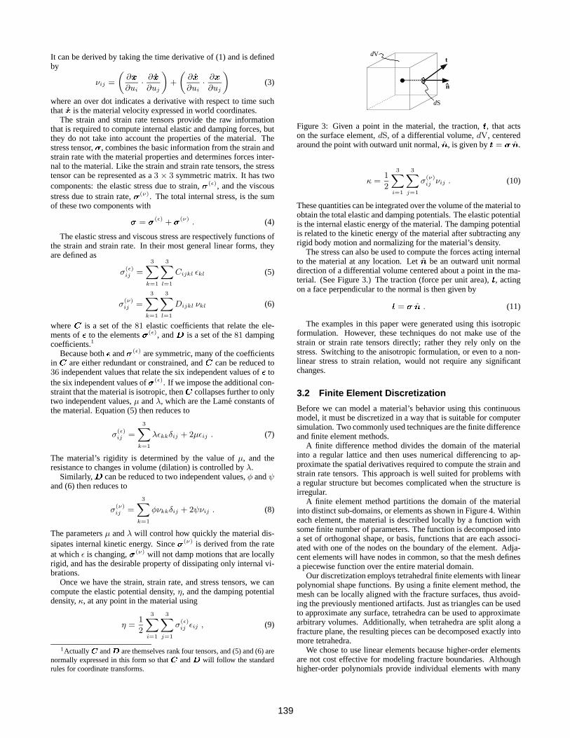
Figure 3: Given a point in the material, the traction,t, that actson the surface element,dS, of a differential volume,dV, centeredaround the point with outward unit normal,n, is given byt = � n.

κ =1

2

3∑i=1

3∑j=1

σ(ν)ij νij . (10)

These quantities can be integrated over the volume of the material toobtain the total elastic and damping potentials. The elastic potentialis the internal elastic energy of the material. The damping potentialis related to the kinetic energy of the material after subtracting anyrigid body motion and normalizing for the material’s density.

The stress can also be used to compute the forces acting internalto the material at any location. Letn be an outward unit normaldirection of a differential volume centered about a point in the ma-terial. (See Figure 3.) The traction (force per unit area),t, actingon a face perpendicular to the normal is then given by

t = � n . (11)

The examples in this paper were generated using this isotropicformulation. However, these techniques do not make use of thestrain or strain rate tensors directly; rather they rely only on thestress. Switching to the anisotropic formulation, or even to a non-linear stress to strain relation, would not require any significantchanges.

3.2 Finite Element Discretization

Before we can model a material’s behavior using this continuousmodel, it must be discretized in a way that is suitable for computersimulation. Two commonly used techniques are the finite differenceand finite element methods.

A finite difference method divides the domain of the materialinto a regular lattice and then uses numerical differencing to ap-proximate the spatial derivatives required to compute the strain andstrain rate tensors. This approach is well suited for problems witha regular structure but becomes complicated when the structure isirregular.

A finite element method partitions the domain of the materialinto distinct sub-domains, or elements as shown in Figure 4. Withineach element, the material is described locally by a function withsome finite number of parameters. The function is decomposed intoa set of orthogonal shape, or basis, functions that are each associ-ated with one of the nodes on the boundary of the element. Adja-cent elements will have nodes in common, so that the mesh definesa piecewise function over the entire material domain.

Our discretization employs tetrahedral finite elements with linearpolynomial shape functions. By using a finite element method, themesh can be locally aligned with the fracture surfaces, thus avoid-ing the previously mentioned artifacts. Just as triangles can be usedto approximate any surface, tetrahedra can be used to approximatearbitrary volumes. Additionally, when tetrahedra are split along afracture plane, the resulting pieces can be decomposed exactly intomore tetrahedra.

We chose to use linear elements because higher-order elementsare not cost effective for modeling fracture boundaries. Althoughhigher-order polynomials provide individual elements with many

139

!!!!!!!!!!!!!!!!!!!!!!!!!!!!!!!!!!!!!!!!!!!!!!!!!!!!!!!!!!!!!!!!!!!!!!!!!!!!!!!!!!!!!!!!!!!!!!!!!!!!!!!!!!!!!!!!!!!!!!!!!!!!!!!!!!!!!!!!!!!!!!!!!!!!!!!!!!

!!!!!!!!!!!!!!!!!!!!!!!!!!!!!!!!!!!!!!!!!!!!!!!!!!!!!!!!!!!!!!!!!!!!!!!!!!!!!!!!!!!!!!!!!!!!!!!!!!!!!!!!!!!!!!!!!!!!!!!!!!!!!!!!!!!!!!!!!!!!!!!!!!!!!!!!!!

(a) ( b)

Figure 4: Tetrahedral mesh for a simple object. In(a), only the ex-ternal faces of the tetrahedra are drawn; in(b) the internal structureis shown.

(a) ( b)m [2]

m [1]

m [3]

m [4]

p [1]

p [2]p [3]

p [4]

v [1]

v [2]

v [3]

v [4]

Figure 5: A tetrahedral element is defined by its four nodes. Eachnode has(a) a location in the material coordinate system and(b) aposition and velocity in the world coordinate system.

degrees of freedom for deformation, they have few degrees of free-dom for modeling fracture because the shape of a fracture is definedas a boundary in material coordinates. In contrast, with linear tetra-hedra, each degree of freedom in the world space corresponds to adegree of freedom in the material coordinates. Furthermore, when-ever an element is created, its basis functions must be computed.For high-degree polynomials, this computation is relatively expen-sive. For systems where the mesh is constant, the cost is amortizedover the course of the simulation. However, as fractures developand parts of the object are remeshed, the computation of basis ma-trices can become significant.

Each tetrahedral element is defined by four nodes. A node hasa position in the material coordinates,m, a position in the worldcoordinates,p, and a velocity in world coordinates,v. We will referto the nodes of a given element by indexing with square brackets.For example,m[2] is the position in material coordinates of theelement’s second node. (See Figure 5.)

Barycentric coordinates provide a natural way to define the linearshape functions within an element. Letb = [b1, b2, b3, b4]T bebarycentric coordinates defined in terms of the element’s materialcoordinates so that[

u

1

]=[m[1]

1

m[2]

1

m[3]

1

m[4]

1

]b . (12)

These barycentric coordinates may also be used to interpolate thenode’s world position and velocity with[

x

1

]=[p[1]

1

p[2]

1

p[3]

1

p[4]

1

]b (13)[

x

1

]=[v[1]

1

v[2]

1

v[3]

1

v[4]

1

]b . (14)

To determine the barycentric coordinates of a point within theelement specified by its material coordinates, we invert (12) andobtain

b = �

[u

1

](15)

where� is defined by

� =[m[1]

1

m[2]

1

m[3]

1

m[4]

1

]−1

. (16)

Combining (15) with (13) and (14) yields functions that interpolatethe world position and velocity within the element in terms of thematerial coordinates:

x(u) = P �

[u

1

](17)

x(u) = V �

[u

1

](18)

whereP andV are defined as

P =[p[1] p[2] p[3] p[4]

](19)

V =[v[1] v[2] v[3] v[4]

]. (20)

Note that the rows of� are the coefficients of the shape functions,and� needs to be computed only when an element is created or thematerial coordinates of its nodes change. For non-degenerate ele-ments, the matrix in (16) is guaranteed to be non-singular, howeverelements that are nearly co-planar will cause� to be ill-conditionedand adversely affect the numerical stability of the system.

Computing the values of� and� within the element requires thefirst partials ofx with respect tou:

∂x

∂ui= P � �i (21)

∂x

∂ui= V � �i (22)

where�i = [δi1 δi2 δi3 0]T . (23)

Because the element’s shape functions are linear, these partials areconstant within the element.

The element will exert elastic and damping forces on its nodes.The elastic force on theith node,f (ε)

[i] , is defined as the partial of theelastic potential density,η, with respect top[i] integrated over the

volume of the element. Given�(ε), �, and the positions in worldspace of the four nodes we can compute the elastic force by

f(ε)

[i] =vol

2

4∑j=1

p[j]

3∑k=1

3∑l=1

βjlβikσ(ε)kl (24)

where

vol =1

6[(m[2]−m[1])× (m[3]−m[1])] · (m[4]−m[1]) . (25)

Similarly, the damping force on theith node,f (ν)

[i] , is defined asthe partial of the damping potential density,κ, with respect tov[i]

integrated over the volume of the element. This quantity can becomputed with

f(ν)

[i] =vol

2

4∑j=1

p[j]

3∑k=1

3∑l=1

βjlβikσ(ν)kl . (26)

Summing these two forces, the total internal force that an elementexerts on a node is

fel[i] =

vol

2

4∑j=1

p[j]

3∑k=1

3∑l=1

βjlβikσkl , (27)

140

and the total internal force acting on the node is obtained by sum-ming the forces exerted by all elements that are attached to the node.

As the element is compressed to less than about30% of its ma-terial volume, the gradient ofη andκ start to vanish causing theresisting forces to fall off. We have not found this to be a problemas even the more squishy of the materials that we have modeledconserve their volume to within a few percent.

Using a lumped mass formulation, the mass contributed by anelement to each one of its nodes is determined by integrating thematerial density,ρ, over the element shape function associated withthat node. In the case of tetrahedral elements with linear shapefunctions, this mass contribution is simplyρ vol/4.

The derivations above are sufficient for a simulation that uses anexplicit integration scheme. Additional work, including computingthe Jacobian of the internal forces, is necessary for implicit integra-tion scheme. (See for example [2] and [3].)

3.3 Collisions

In addition to the forces internal to the material, the system com-putes collision forces. The collision forces are computed using apenalty method that is applied when two elements intersect or if anelement violates another constraint such as the ground. Althoughpenalty methods are often criticized for creating stiff equations, wehave found that for the materials we are modeling the internal forcesare at least as stiff as the penalty forces. Penalty forces have theadvantage of being very fast to compute. We have experimentedwith two different penalty criteria: node penetration and overlapvolume. The examples presented in this paper were computed withthe node penetration criteria; additional examples on the conferenceproceedings CD-ROM were computed with the overlap volume cri-teria.

The node penetration criteria sets the penalty force to be pro-portional to the distance that a node has penetrated into anotherelement. The penalty force acts in the direction normal to the pene-trated surface. The reaction force is distributed over the penetratedelement’s nodes so that the net force and moment are the negation ofthe penalty force and moment acting at the penetrating node. Thistest will not catch all collisions, and undetected intersecting tetra-hedra may become locked together. It is however, fast to compute,easy to implement, and adequate for situations that do not involvecomplex collision interactions.

The overlap volume criteria is more robust than the node pene-tration method, but it is also slower to compute and more complexto implement. The intersection of two tetrahedral elements is com-puted by clipping the faces of each tetrahedron against the other.The resulting polyhedron is then used to compute the volume andcenter of mass of the intersecting region. The area weighted nor-mals of the faces of the polyhedron that are contributed by one ofthe tetrahedra are summed to compute the direction that the penaltyforce acts in. A similar computation can be performed for the othertetrahedra, or equivalently the direction can be negated. Providedthat neither tetrahedra is completely contained within the other, thiscriteria is more robust than the node penetration criteria. Addition-ally, the forces computed with this method do not depend on theobject tessellation.

Computing the intersections within the mesh can be very expen-sive, and we use a bounding hierarchy scheme with cached traver-sals to help reduce this cost.

4 Fracture Modeling

Our fracture model is based on the theory of linear elastic fracturemechanics [1]. The primary distinction between this and other the-

!!!!!!!!!!!!!!!!!!!!!!!!!!!!!!!!!!!!

I !!!!!!!!!!!!!!!!!!!!!!!!!!!!!!

IIIII!!!!!!!!!!!!!!!!!!!!!!!!!!!!!!

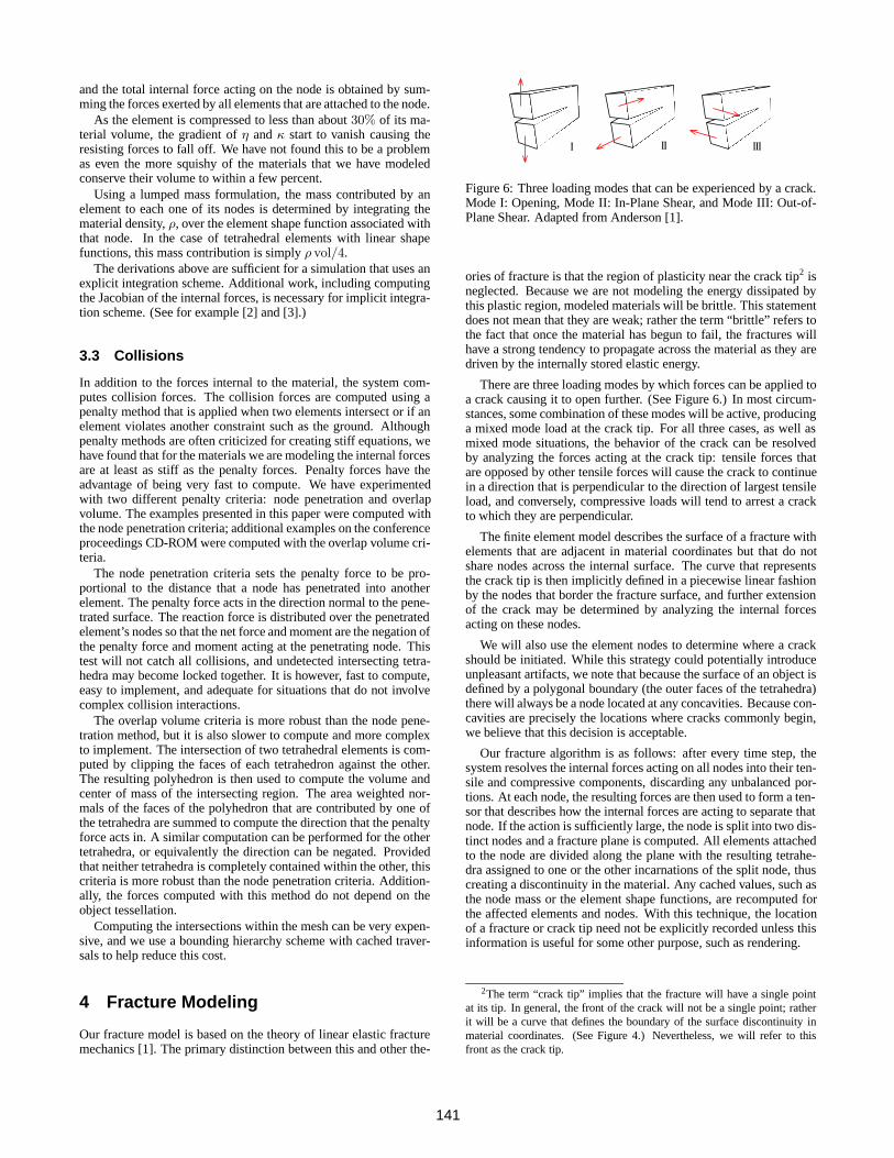
Figure 6: Three loading modes that can be experienced by a crack.Mode I: Opening, Mode II: In-Plane Shear, and Mode III: Out-of-Plane Shear. Adapted from Anderson [1].

ories of fracture is that the region of plasticity near the crack tip2 isneglected. Because we are not modeling the energy dissipated bythis plastic region, modeled materials will be brittle. This statementdoes not mean that they are weak; rather the term “brittle” refers tothe fact that once the material has begun to fail, the fractures willhave a strong tendency to propagate across the material as they aredriven by the internally stored elastic energy.

There are three loading modes by which forces can be applied toa crack causing it to open further. (See Figure 6.) In most circum-stances, some combination of these modes will be active, producinga mixed mode load at the crack tip. For all three cases, as well asmixed mode situations, the behavior of the crack can be resolvedby analyzing the forces acting at the crack tip: tensile forces thatare opposed by other tensile forces will cause the crack to continuein a direction that is perpendicular to the direction of largest tensileload, and conversely, compressive loads will tend to arrest a crackto which they are perpendicular.

The finite element model describes the surface of a fracture withelements that are adjacent in material coordinates but that do notshare nodes across the internal surface. The curve that representsthe crack tip is then implicitly defined in a piecewise linear fashionby the nodes that border the fracture surface, and further extensionof the crack may be determined by analyzing the internal forcesacting on these nodes.

We will also use the element nodes to determine where a crackshould be initiated. While this strategy could potentially introduceunpleasant artifacts, we note that because the surface of an object isdefined by a polygonal boundary (the outer faces of the tetrahedra)there will always be a node located at any concavities. Because con-cavities are precisely the locations where cracks commonly begin,we believe that this decision is acceptable.

Our fracture algorithm is as follows: after every time step, thesystem resolves the internal forces acting on all nodes into their ten-sile and compressive components, discarding any unbalanced por-tions. At each node, the resulting forces are then used to form a ten-sor that describes how the internal forces are acting to separate thatnode. If the action is sufficiently large, the node is split into two dis-tinct nodes and a fracture plane is computed. All elements attachedto the node are divided along the plane with the resulting tetrahe-dra assigned to one or the other incarnations of the split node, thuscreating a discontinuity in the material. Any cached values, such asthe node mass or the element shape functions, are recomputed forthe affected elements and nodes. With this technique, the locationof a fracture or crack tip need not be explicitly recorded unless thisinformation is useful for some other purpose, such as rendering.

2The term “crack tip” implies that the fracture will have a single pointat its tip. In general, the front of the crack will not be a single point; ratherit will be a curve that defines the boundary of the surface discontinuity inmaterial coordinates. (See Figure 4.) Nevertheless, we will refer to thisfront as the crack tip.

141

4.1 Force Decomposition

The forces acting on a node are decomposed by first separatingthe element stress tensors into tensile and compressive components.For a given element in the mesh, letvi(�), with i ∈ {1, 2, 3}, be theith eigenvalue of�, and letni(�) be the corresponding unit lengtheigenvector. Positive eigenvalues correspond to tensile stresses andnegative ones to compressive stresses. Since� is real and symmet-ric, it will have three real, not necessarily unique, eigenvalues. Inthe case where an eigenvalue has multiplicity greater than one, theeigenvectors are selected arbitrarily to orthogonally span the appro-priate subspace [13].

Given a vectora in<3, we can construct a3× 3 symmetric ma-trix, m(a) that has|a| as an eigenvalue witha as the correspondingeigenvector, and with the other two eigenvalues equal to zero. Thismatrix is defined by

m(a) =

{aaT/|a| : a 6= 0

0 : a = 0 .(28)

The tensile component,�+, and compressive component,�−,of the stress within the element can now be computed by

�+ =

3∑i=1

max(0, vi(�)) m(ni(�)) (29)

�− =

3∑i=1

min(0, vi(�)) m(ni(�)) . (30)

Using this decomposition, the force that an element exerts on anode can be separated into a tensile component,f+

[i], and a com-

pressive component,f−[i]. This separation is done by reevaluating

the internal forces exerted on the nodes using (27) with�+ or �−

substituted for�. Thus the tensile component is

f+[i] =

vol

2

4∑j=1

p[j]

3∑k=1

3∑l=1

βjlβikσ+kl . (31)

The compressive component can be computed similarly, but be-cause� = �+ + �−, it can be computed more efficiently usingf [i] = f+

[i] + f−[i].Each node will now have a set of tensile and a set of compressive

forces that are exerted by the elements attached to it. For a givennode, we denote these sets as{f+} and{f−} respectively. Theunbalanced tensile load,f+ is simply the sum over{f+}, and theunbalanced compressive load,f−, is the sum over{f−}.

4.2 The Separation Tensor

We describe the forces acting at the nodes using a stress variant thatwe call the separation tensor,&. The separation tensor is formedfrom the balanced tensile and compressive forces acting at eachnode and is computed by

& =1

2

−m(f+)+∑

f∈{f+}

m(f) + m(f−)−∑

f∈{f−}

m(f)

. (32)

It does not respond to unbalanced actions that would produce a rigidtranslation, and is invariant with respect to transformations of boththe material and world coordinate systems.

The separation tensor is used directly to determine whether afracture should occur at a node. Letv+ be the largest positive eigen-value of&. If v+ is greater than the material toughness,τ , then the

(a) (c)( b)

Figure 7: Diagram showing how an element is split by the fractureplane. (a) The initial tetrahedral element.(b) The splitting nodeand fracture plane are shown in blue.(c) The element is split alongthe fracture plane into two polyhedra that are then decomposed intotetrahedra. Note that the two nodes created from the splitting nodeare co-located, the geometric displacement shown in(c) only illus-trates the location of the fracture discontinuity.

(a) ( b) (c)

Figure 8: Elements that are adjacent to an element that has beensplit by a fracture plane must also be split to maintain mesh consis-tency. (a) Neighboring tetrahedra prior to split.(b) Face neighborafter split.(c) Edge neighbor after split.

material will fail at the node. The orientation in world coordinatesof the fracture plane is perpendicular ton+, the eigenvalue of&that corresponds tov+. In the case where multiple eigenvalues aregreater thanτ , multiple fracture planes may be generated by firstgenerating the plane for the largest value, remeshing (see below),and then recomputing the new value for& and proceeding as above.

4.3 Local Remeshing

Once the simulation has determined the location and orientation ofa new fracture plane, the mesh must be modified to reflect the newdiscontinuity. It is important that the orientation of the fracture bepreserved, as approximating it with the existing element boundarieswould create undesirable artifacts. To avoid this potential difficulty,the algorithm remeshes the local area surrounding the new fractureby splitting elements that intersect the fracture plane and modifyingneighboring elements to ensure that the mesh stays self-consistent.

First, the node where the fracture originates is replicated so thatthere are now two nodes,n+ andn− with the same material posi-tion, world position, and velocity. The masses will be recalculatedlater. The discontinuity passes “between” the two co-located nodes.The positive side of the fracture plane is associated withn+ and thenegative side withn−.

Next, all elements that were attached to the original node are ex-amined, comparing the world location of their nodes to the fractureplane. If an element is not intersected by the fracture plane, thenit is reassigned to eithern+ or n− depending on which side of theplane it lies.

If the element is intersected by the fracture plane, it is split alongthe plane. (See Figure 7.) A new node is created along each edgethat intersects the plane. Because all elements must be tetrahedra, ingeneral each intersected element will be split into three tetrahedra.One of the tetrahedra will be assigned to one side of the plane andthe other two to the other side. Because the two tetrahedra thatare on the same side of the plane both share eithern+ or n−, thediscontinuity does not pass between them.

In addition to the elements that were attached to the originalnode, it may be necessary to split other elements so that the mesh

142

Figure 9: Two adobe walls that are struck by wrecking balls. Both walls are attached to the ground. The ball in the second row has50×the mass of the first. Images are spaced apart133.3 ms in the first row and66.6 ms in the second. The rightmost images show the finalconfigurations.

a b

dc

Figure 10: Mesh for adobe wall.(a) The facing surface of the initialmesh used to generate the wall shown in Figure 9.(b) The mesh af-ter being struck by the wrecking ball, reassembled.(c) Same as (b),with the cracks emphasized.(d) Internal fractures shown as wire-frame.

stays consistent. In particular, an element must be split if the face oredge between it and another element that was attached to the orig-inal node has been split. (See Figure 8.) To prevent the remeshingfrom cascading across the entire mesh, these splits are done so thatthe new tetrahedra use only the original nodes and the nodes cre-ated by the intersection splits. Because no new nodes are created,the effect of the local remeshing is limited to the elements that areattached to the node where the fracture originated and their imme-diate neighbors. Because the tetrahedra formed by the secondarysplits do not attach to eithern+ or n−, the discontinuity does notpass between them.

Finally, after the local remeshing has been completed, anycached values that have become invalid must be recomputed. Inour implementation, these values include the element basis matrix,�, and the node masses.

Two additional subtleties must also be considered. The firstsubtlety occurs when an intersection split involves an edge thatis formed only by tetrahedra attached to the node where the crackoriginated. When this happens, the fracture has reached a boundaryin the material, and the discontinuity should pass through the edge.Remeshing occurs as above, except that two nodes are created onthe edge and one is assigned to each side of the discontinuity.

Second, the fracture plane may pass arbitrarily close to an exist-ing node producing arbitrarily ill-conditioned tetrahedra. To avoidthis, we employ two thresholds, one the distance between the frac-

ture plane and an existing node, and the other on the angle betweenthe fracture plane and a line from the node where the split origi-nated to the existing node. If either of these thresholds are not met,then the intersection split is snapped to the existing node. In ourresults, we have used thresholds of5 mm and0.1 radians.

5 Results and Discussion

To demonstrate some of the effects that can be generated with thisfracture technique, we have animated a number of scenes that in-volve objects breaking. Figure 1 shows a plate of glass that has hada heavy weight dropped on it. The area in the immediate vicinityof the impact has been crushed into many small fragments. Furtheraway from the weight, a pattern of radial cracks has developed.

Figure 9 shows two walls being struck by wrecking balls. Inthe first sequence, the wall develops a network of cracks as it ab-sorbs most of the ball’s energy during the initial impact. In the sec-ond sequence, the ball’s mass is50× greater, and the wall shatterswhen it is struck. The mesh used to generate the wall sequences isshown in Figure 10. The initial mesh contains only338 nodes and1109 elements. By the end of the sequence, the mesh has grownto 6892 nodes and8275 elements. These additional nodes and el-ements are created where fractures occur; a uniform mesh wouldrequire many times this number of nodes and elements to achieve asimilar result.

Figure 11 shows the final frames from four animations of bowlsthat were dropped onto a hard surface. Other than the toughness,τ , of the material, the four simulations are identical. The first bowldevelops only a few cracks; the weakest breaks into many pieces.

Because this system works with solid tetrahedral volumes ratherthan with the polygonal boundary representations created by mostmodeling packages, boundary models must be converted beforethey can be used. A number of systems are available for creatingtetrahedral meshes from polygonal boundaries. The models thatwe used in these examples were generated either from a CSG de-scription or a polygonal boundary representation using NETGEN,a publicly available mesh generation package [16].

Although our approach avoids the “jaggy” artifacts in the frac-ture patterns caused by the underlying mesh, there remain ways inwhich the results of a simulation are influenced by the mesh struc-ture. The most obvious is that the deformation of the material islimited by the degrees of freedom in the mesh, which in turn limitshow the material can fracture. This limitation will occur with anydiscrete system. The technique also limits where a fracture may ini-

143

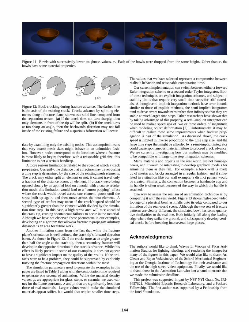
Figure 11: Bowls with successively lower toughness values,τ . Each of the bowls were dropped from the same height. Other thanτ , thebowls have same material properties.

θopen

θturn θturn

θopen

(a) ( b)

Figure 12: Back-cracking during fracture advance. The dashed lineis the axis of the existing crack. Cracks advance by splitting ele-ments along a fracture plane, shown as a solid line, computed fromthe separation tensor.(a) If the crack does not turn sharply, thenonly elements in front of the tip will be split.(b) If the crack turnsat too sharp an angle, then the backwards direction may not fallinside of the existing failure and a spurious bifurcation will occur.

tiate by examining only the existing nodes. This assumption meansthat very coarse mesh sizes might behave in an unintuitive fash-ion. However, nodes correspond to the locations where a fractureis most likely to begin; therefore, with a reasonable grid size, thislimitation is not a serious handicap.

A more serious limitation is related to the speed at which a crackpropagates. Currently, the distance that a fracture may travel duringa time step is determined by the size of the existing mesh elements.The crack may either split an element or not; it cannot travel onlya fraction of the distance across an element. If a crack were beingopened slowly by an applied load on a model with a coarse resolu-tion mesh, this limitation would lead to a “button popping” effectwhere the crack would travel across one element, pause until thestress built up again, and then move across the next element. Asecond type of artifact may occur if the crack’s speed should besignificantly greater than the element width divided by the simula-tion time step. In this case, a high stress area will race ahead ofthe crack tip, causing spontaneous failures to occur in the material.Although we have not observed these phenomena in our examples,developing an algorithm that allows a fracture to propagate arbitrarydistances is an area for future work.

Another limitation stems from the fact that while the fractureplane’s orientation is well defined, the crack tip’s forward directionis not. As shown in Figure 12, if the cracks turns at an angle greaterthan half the angle at the crack tip, then a secondary fracture willdevelop in the opposite direction to the crack’s advance. While thiseffect is likely present in some of our examples, it does not appearto have a significant impact on the quality of the results. If the arti-facts were to be a problem, they could be suppressed by explicitlytracking the fracture propagation directions within the mesh.

The simulation parameters used to generate the examples in thispaper are listed in Table 1 along with the computation time requiredto generate one second of animation. While the material densityvalues,ρ, are appropriate for glass, stone, or ceramic, we used val-ues for the Lam´e constants,λ andµ, that are significantly less thanthose of real materials. Larger values would make the simulatedmaterials appear stiffer, but would also require smaller time steps.

The values that we have selected represent a compromise betweenrealistic behavior and reasonable computation time.

Our current implementation can switch between either a forwardEuler integration scheme or a second order Taylor integrator. Bothof these techniques are explicit integration schemes, and subject tostability limits that require very small time steps for stiff materi-als. Although semi-implicit integration methods have error boundssimilar to those of explicit methods, the semi-implicit integratorstend to drive errors towards zero rather than infinity so that they arestable at much larger time steps. Other researchers have shown thatby taking advantage of this property, a semi-implicit integrator canbe used to realize speed ups of two or three orders of magnitudewhen modeling object deformation [2]. Unfortunately, it may bedifficult to realize these same improvements when fracture prop-agation is part of the simulation. As discussed above, the crackspeed is limited in inverse proportion to the time step size, and thelarge time steps that might be afforded by a semi-implicit integratorcould cause spontaneous material failure to proceed crack advance.We are currently investigating how our methods may be modifiedto be compatible with large time step integration schemes.

Many materials and objects in the real world are not homoge-neous, and it would be interesting to develop graphical models foranimating them as they fail. For example, a brick wall is madeup of mortar and bricks arranged in a regular fashion, and if simu-lated in a situation like our wall example, a distinct pattern wouldbe created. Similarly, the connection between a handmade cup andits handle is often weak because of the way in which the handle isattached.

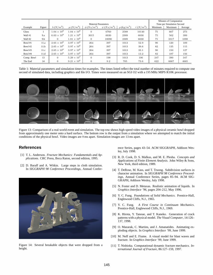
One way to assess the realism of an animation technique is bycomparing it with the real world. Figure 13 shows high-speed videofootage of a physical bowl as it falls onto its edge compared to ourimitation of the real-world scene. Although the two sets of fracturepatterns are clearly different, the simulated bowl has some qualita-tive similarities to the real one. Both initially fail along the leadingedge where they strike the ground, and subsequently develop verti-cal cracks before breaking into several large pieces.

Acknowledgments

The authors would like to thank Wayne L. Wooten of Pixar Ani-mation Studios for lighting, shading, and rendering the images formany of the figures in this paper. We would also like to thank AriGlezer and Bojan Vukasinovic of the School Mechanical Engineer-ing at the Georgia Institute of Technology for their assistance andthe use of the high-speed video equipment. Finally, we would liketo thank those in the Animation Lab who lent a hand to ensure thatwe made the submission deadline.

This project was supported in part by NSF NYI Grant No. IRI-9457621, Mitsubishi Electric Research Laboratory, and a PackardFellowship. The first author was supported by a Fellowship fromthe Intel Foundation.

144

Minutes of ComputationMaterial Parameters Time per Simulation Second

Example Figure λ (N/m2) µ (N/m2) φ (Ns/m2) ψ (Ns/m2) ρ (kg/m3) τ (N/m2) Minimum Maximum Average

Glass 1 1.04× 108 1.04 × 108 0 6760 2588 10140 75 667 273

Wall #1 9.a 6.03× 108 1.21 × 108 3015 6030 2309 6030 75 562 399

Wall #2 9.b 0 1.81 × 108 0 18090 2309 6030 75 2317 1098

Bowl #1 11.a 2.65× 106 3.97 × 106 264 397 1013 52.9 90 120 109

Bowl #2 11.b 2.65× 106 3.97 × 106 264 397 1013 39.6 82 135 115

Bowl #3 11.c 2.65× 106 3.97 × 106 264 397 1013 33.1 90 150 127

Bowl #4 11.d 2.65× 106 3.97 × 106 264 397 1013 13.2 82 187 156

Comp. Bowl 13 0 5.29 × 107 0 198 1013 106 247 390 347

The End 14 0 9.21 × 106 0 9.2 705 73.6 622 6667 4665

Table 1: Material parameters and simulation times for examples. The times listed reflect the total number of minutes required to compute onesecond of simulated data, including graphics and file I/O. Times were measured on an SGI O2 with a195 MHz MIPS R10K processor.

Figure 13: Comparison of a real-world event and simulation. The top row shows high-speed video images of a physical ceramic bowl droppedfrom approximately one meter onto a hard surface. The bottom row is the output from a simulation where we attempted to match the initialconditions of the physical bowl. Video images are8 ms apart. Simulation images are13 ms apart.

References

[1] T. L. Anderson.Fracture Mechanics: Fundamentals and Ap-plications. CRC Press, Boca Raton, second edition, 1995.

[2] D. Baraff and A. Witkin. Large steps in cloth simulation.In SIGGRAPH 98 Conference Proceedings, Annual Confer-

Figure 14: Several breakable objects that were dropped from aheight.

ence Series, pages 43–54. ACM SIGGRAPH, Addison Wes-ley, July 1998.

[3] R. D. Cook, D. S. Malkus, and M. E. Plesha.Concepts andApplications of Finite Element Analysis. John Wiley & Sons,New York, third edition, 1989.

[4] T. DeRose, M. Kass, and T. Truong. Subdivision surfaces incharacter animation. InSIGGRAPH 98 Conference Proceed-ings, Annual Conference Series, pages 85–94. ACM SIG-GRAPH, Addison Wesley, July 1998.

[5] N. Foster and D. Metaxas. Realistic animation of liquids. InGraphics Interface ’96, pages 204–212, May 1996.

[6] Y. C. Fung. Foundations of Solid Mechanics. Prentice-Hall,Englewood Cliffs, N.J., 1965.

[7] Y. C. Fung. A First Course in Continuum Mechanics.Prentice-Hall, Englewood Cliffs, N.J., 1969.

[8] K. Hirota, Y. Tanoue, and T. Kaneko. Generation of crackpatterns with a physical model.The Visual Computer, 14:126–137, 1998.

[9] O. Mazarak, C. Martins, and J. Amanatides. Animating ex-ploding objects. InGraphics Interface ’99, June 1999.

[10] M. Neff and E. Fiume. A visual model for blast waves andfracture. InGraphics Interface ’99, June 1999.

[11] T. Nishioka. Computational dynamic fracture mechanics.In-ternational Journal of Fracture, 86:127–159, 1997.

145

[12] A. Norton, G. Turk, B. Bacon, J. Gerth, and P. Sweeney. An-imation of fracture by physical modeling.The Visual Com-puter, 7:210–217, 1991.

[13] W. H. Press, B. P. Flannery, S. A. Teukolsky, and W. T. Vet-terling. Numerical Recipes in C. Cambridge University Press,second edition, 1994.

[14] B. Robertson. Antz-piration. Computer Graphics World,21(10), 1998.

[15] B. Robertson. Meet Geri: The new face of animation.Com-puter Graphics World, 21(2), 1998.

[16] J. Schoberl. NETGEN – An advancing front 2D/3D–meshgenerator based on abstract rules.Computing and Visualiza-tion in Science, 1:41–52, 1997.

[17] D. Terzopoulos. Regularization of inverse visual problems in-volving discontinuities.IEEE Transactions on Pattern Analy-sis and Machine Intelligence, 8(4):413–424, July 1986.

[18] D. Terzopoulos and K. Fleischer. Deformable models.TheVisual Computer, 4:306–331, 1988.

[19] D. Terzopoulos and K. Fleischer. Modeling inelastic deforma-tion: Viscoelasticity, plasticity, fracture. InComputer Graph-ics (SIGGRAPH ’88 Proceedings), volume 22, pages 269–278, August 1988.

146