graphical presentation and numerical modelling of ...janousek/rkurz/pdf_eng/r_prague... · (visual...
TRANSCRIPT
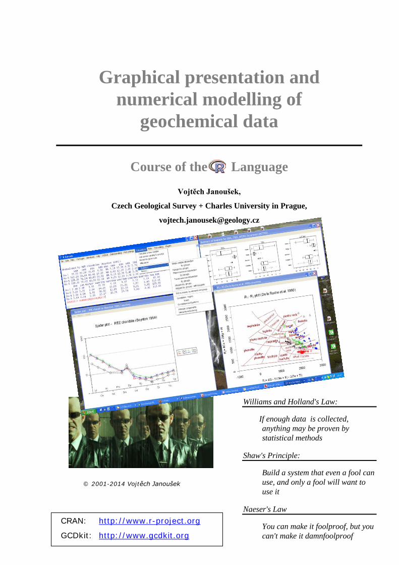
Graphical presentation and numerical modelling of
geochemical data
Course of the Language
Vojtěch Janoušek,
Czech Geological Survey + Charles University in Prague,
Williams and Holland's Law:
If enough data is collected, anything may be proven by statistical methods
Shaw's Principle:
Build a system that even a fool can use, and only a fool will want to use it
Naeser's Law
You can make it foolproof, but you can't make it damnfoolproof
© 2001-2014 Vojtěch Janoušek
CRAN: http://www.r-project.org
GCDkit: http://www.gcdkit.org
1/2
CRAN: http://www.r-project.org
Web of this course: http://petrol.natur.cuni.cz/~janousek/Rkurz/
Selected references
CLARKE D. 1994. NewPet for DOS. Accessed November 11, 2003, at URL ftp://www.esd.mun.ca/pub/geoprogs/np940107.exe.
JANOUŠEK V. 2000. NORMAN, a QuickBasic programme for petrochemical re-calculation of whole-rock major-element analyses on IBM PC. J. Czech Geol. Soc., 46: 9–13.
MELÍN M. & KUNST M. 1992. MinCalc development kit 2.1. Geol. ústav Akad. věd, Prague. PETRELLI M., POLI G., PERUGINI D. & PECCERILLO A. 2005. PetroGraph: A new
software to visualize, model, and present geochemical data in igneous petrology. Geochemistry Geophysics Geosystems 6: 15 pp.
RICHARD L.R. 1995. MinPet: Mineralogical and petrological data processing system, version 2.02. MinPet Geological Software, Québec, Canada.
SIDDER G. B. 1994. Petro.calc.plot, Microsoft Excel macros to aid petrologic interpretation: Computers & Geosciences, 20: 1041–1061.
STORMER J. C. & NICHOLLS J. 1978. XLFRAC: a program for the interactive testing of magmatic differentiation models. Computers & Geosciences 4: 143–159.
SU Y. J., LANGMUIR C. H. & ASIMOW P. D. 2003. PetroPlot: A plotting and data mana-gement tool set for Microsoft Excel. Geochemistry Geophysics Geosystems 4: 14 pp.
WANG X., MA W., GAO, S. & KE, L. 2008. GCDPlot: An extensible Microsoft Excel VBA program for geochemical discrimination diagrams. Computers & Geosciences, 34: 1964–1969.
ZHOU J. & LI X. 2006. GeoPlot: An Excel VBA program for geochemical data plotting. Computers Geosciences 32: 554–560.
1.1 Spreadsheets (MS Excel, Quattro Pro …) Advantages:
Widespread Easy to use Zero extra costs
Disadvantages: Scarcity of dedicated geochemical applications (but see Sidder, 1994; Su et al., 2003; Zhou & Li, 2006) Low quality of graphic output Limited protection of the primary data Complex, prone to errors Low efficiency for repeated tasks
SW for geochemical recalculations and graphics
1/3
1.2 Dedicated software
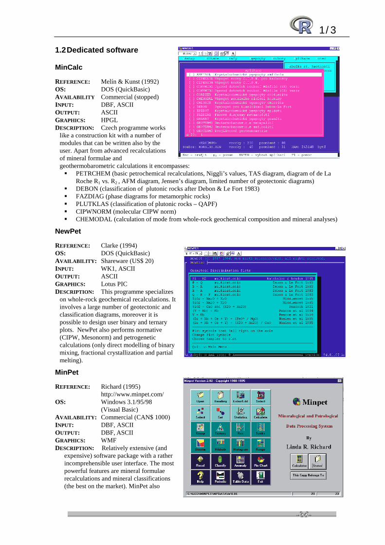
MinCalc
REFERENCE: Melín & Kunst (1992) OS: DOS (QuickBasic) AVAILABILITY Commercial (stopped) INPUT: DBF, ASCII OUTPUT: ASCII GRAPHICS: HPGL DESCRIPTION: Czech programme works
like a construction kit with a number of modules that can be written also by the user. Apart from advanced recalculations of mineral formulae and geothermobarometric calculations it encompasses: PETRCHEM (basic petrochemical recalculations, Niggli’s values, TAS diagram, diagram of de La
Roche R1 vs. R2 , AFM diagram, Jensen’s diagram, limited number of geotectonic diagrams) DEBON (classification of plutonic rocks after Debon & Le Fort 1983) FAZDIAG (phase diagrams for metamorphic rocks) PLUTKLAS (classification of plutonic rocks – QAPF) CIPWNORM (molecular CIPW norm) CHEMODAL (calculation of mode from whole-rock geochemical composition and mineral analyses)
NewPet
REFERENCE: Clarke (1994) OS: DOS (QuickBasic) AVAILABILITY: Shareware (US$ 20) INPUT: WK1, ASCII OUTPUT: ASCII GRAPHICS: Lotus PIC DESCRIPTION: This programme specializes
on whole-rock geochemical recalculations. It involves a large number of geotectonic and classification diagrams, moreover it is possible to design user binary and ternary plots. NewPet also performs normative (CIPW, Mesonorm) and petrogenetic calculations (only direct modelling of binary mixing, fractional crystallization and partial melting).
MinPet
REFERENCE: Richard (1995) http://www.minpet.com/
OS: Windows 3.1/95/98 (Visual Basic)
AVAILABILITY: Commercial (CAN$ 1000) INPUT: DBF, ASCII OUTPUT: DBF, ASCII GRAPHICS: WMF DESCRIPTION: Relatively extensive (and
expensive) software package with a rather incomprehensible user interface. The most powerful features are mineral formulae recalculations and mineral classifications (the best on the market). MinPet also
1/4
STANDARD MODULES
The Main menu
NORMAN.EXEInitialization
module
SAVE.EXEFile output
module
INSTALL.EXEInstallation
module
(External graphic programme)
DIRECT.EXEFile manager
module
CALC.EXECalculation
module
oad data filedit/enter dataalculationsisplay resultsrint all/selectedave resultsptions changeuit to DOS
LECDPSOQ
* *****
**x
y
USER-DEFINED FUNCTIONS
dBASENewPetASCII
dBASENewPetASCII
dBASENewPetASCII
NORMANNORMAN
MAIN.EXECore module
involves many whole-rock classification and geotectonic plots. Advanced are spiderplots. Apart from that it is possible to obtain simple descriptive statistics characterizing distribution of individual major and trace elements. This programme performs no petrogenetic or normative calculations, with a sole exception of the CIPW norm.
IgPet
REFERENCE: http://www.aist.go.jp/GSJ/~jdehn/vpetro/igpet.htm OS: Windows 3.1/95/98 (Visual
Basic) AVAILABILITY: Commercial
(Individual: US$ 199, Site: US$ 398/498)
INPUT: DBF, ASCII OUTPUT: DBF, ASCII GRAPHICS: WMF DESCRIPTION: Relatively short and elegant
programme with intuitive user interface. Involves a limited number of classification and geotectonic diagrams, somewhat larger is the selection of spiderplots. Besides that, it is possible to design user-defined binary and ternary plots. A speciality is interactive identification of the individual data points as well as plotting of regression lines and trends caused by a variety of petrogenetic processes (e.g., fractional crystallization, AFC, binary mixing, zone refining…). An independent module serves for a major-element based inverse modelling of fractional crystallization (input: composition of parental and fractionated melts, mineral analyses of the presumed crystallizing phases; output: their proportions in cumulate and degree of fractional crystallization). The only norm IgPet is capable of calculating is CIPW.
Norman
REFERENCE: Janoušek (1999, 2000) OS: DOS (QuickBasic) AVAILABILITY: Freeware INPUT: DBF, ASCII OUTPUT: DBF, ASCII GRAPHICS: – DESCRIPTION: Norman focuses solely on
normative recalculations of the whole-rock major-element analyses. In this respect it offers by far the most extensive list of calculation schemes. E.g. CIPW norm (including its variation with amphibole and biotite), Catanorm, Improved Granite Mesonorm, Niggli’s values, multicationic parameters of Debon & Le Fort, De la Roche et al. etc. Modular design makes Norman extensible by user additions; the new modules can be either simple text scripts or full-blown QuickBasic programmes. Its development is long stopped in favour of the GCDkit package (see below).
1/5
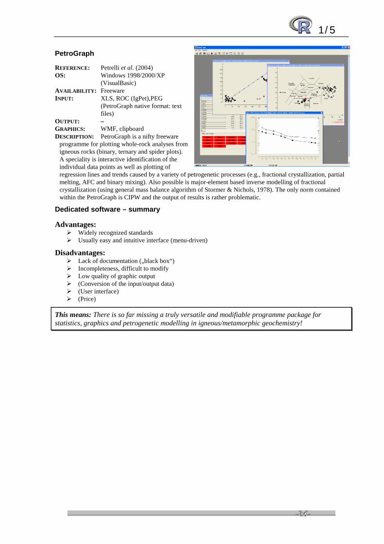
PetroGraph
REFERENCE: Petrelli et al. (2004) OS: Windows 1998/2000/XP
(VisualBasic) AVAILABILITY: Freeware INPUT: XLS, ROC (IgPet),PEG
(PetroGraph native format: text files)
OUTPUT: – GRAPHICS: WMF, clipboard DESCRIPTION: PetroGraph is a nifty freeware
programme for plotting whole-rock analyses from igneous rocks (binary, ternary and spider plots). A speciality is interactive identification of the individual data points as well as plotting of regression lines and trends caused by a variety of petrogenetic processes (e.g., fractional crystallization, partial melting, AFC and binary mixing). Also possible is major-element based inverse modelling of fractional crystallization (using general mass balance algorithm of Stormer & Nichols, 1978). The only norm contained within the PetroGraph is CIPW and the output of results is rather problematic.
Dedicated software – summary
Advantages: Widely recognized standards Usually easy and intuitive interface (menu-driven)
Disadvantages: Lack of documentation („black box“) Incompleteness, difficult to modify Low quality of graphic output (Conversion of the input/output data) (User interface) (Price)
This means: There is so far missing a truly versatile and modifiable programme package for statistics, graphics and petrogenetic modelling in igneous/metamorphic geochemistry!
1/6
Selected references:
BECKER R.A., CHAMBERS J.M. & WILKS A.R. 1988. The New S Language. Chapman & Hall, London.
GRUNSKY, E. C., 2002. R: a data analysis and statistical programming environment – an emerging tool for the geosciences: Computers & Geosciences, 28: 1219–1222.
HORNIK K. 2012. The R FAQ. Accessed October 17, 2012, at URL http://cran.r-project.org/doc/FAQ/R-FAQ.html.
IHAKA R. & GENTLEMAN R. 1996. R: A language for data analysis and graphics. Journal of Computational and Graphical Statistics, 5: 299–344.
JANOUŠEK V., FARROW C. M. & ERBAN V., 2006. Interpretation of whole-rock geochemical data in igneous geochemistry: introducing Geochemical Data Toolkit (GCDkit). Journal of Petrology 47: 1255–1259.
VENABLES, W.N. & RIPLEY, B.D. 1999. Modern Applied Statistics with S-PLUS. Springer, New York.
VENABLES W.N., SMITH D. M. & R DEVELOPMENT CORE TEAM 2012. An Introduction to R. Notes on R: A Programming Environment for Data Analysis and Graphics. Version 2.15.1 (22 June 2012). Accessed October 17, 2012, at URL http://cran.r-project.org/doc/manuals/R-intro.pdf.
1.3 R = a viable alternative to dedicated geochemical software/spreadsheets
R is a programming language/environment for statistical calculations and computer graphics: Ihaka & Gentleman (1996), Dept. Statistics, Auckland, New Zealand;
Since 1997 is developed by R Core Team “of about a dozen people”, Internet cooperation + CRAN Syntax is based on commercially successful S language by Becker, Chambers & Wilks, developed in
AT&T Bell Laboratories (Becker et al. 1988); now distributed as S Plus by Insightful Free and open-sourced software distributed under the GNU copyleft Available for Windows, Unix and Mac OS. Current version 2.15.1
(1.0 was published on 29 February 2000)
Advantages:
Price (= zero), painless installation Easy data input (no fixed data structure, allowed are missing values = NA) Built-in arithmetic, database and a statistical functions High-quality graphical output (PostScript, WMF, HPGL, BMP…) Power, lucidity (structured, high-level language) Interactive as well as batch regime Expandability (StatLib) Portability of the code
Disadvantages:
New SW – not yet widespread Unusual and complex syntax (“steep learning curve”) For serious work is necessary a programming knowledge (= psychological barrier to most of our
colleagues)
Fundamentals of R
1/7
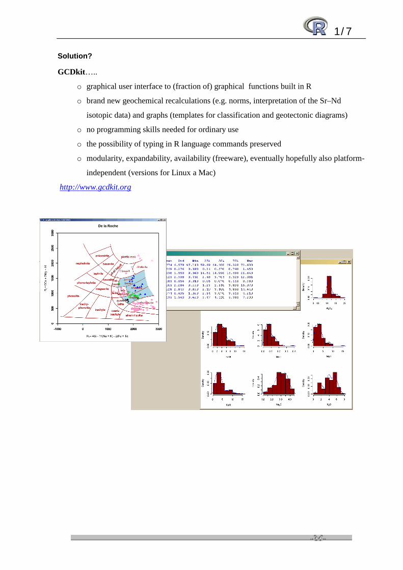
Solution?
GCDkit…..
o graphical user interface to (fraction of) graphical functions built in R
o brand new geochemical recalculations (e.g. norms, interpretation of the Sr–Nd
isotopic data) and graphs (templates for classification and geotectonic diagrams)
o no programming skills needed for ordinary use
o the possibility of typing in R language commands preserved
o modularity, expandability, availability (freeware), eventually hopefully also platform-
independent (versions for Linux a Mac)
http://www.gcdkit.org
1/8
1.4 Installation of R Download the current version of R from the CRAN site (http://cran.r-project.org/), the name contains a
version number, for 2.2 it was R-2.2.0-win32.exe Run the file R-XXX-win32.exe and select the required items as well as the target directory.
1.5 Starting and terminating the R session After double clicking the file RGUI.EXE opens “R Console”, a text window serving for entry of commands and display of textual output. The system prints a number of messages, the most important of which is the last line with a prompt, showing that the R environment is awaiting your commands. Apart from the R Console, one or more windows for graphical output can be active. To end a R session one can invoke a menu item File|Exit or type:
> q()
1.6 Help and documentation The R environment provides help in several forms – pure text (ASCII), Windows Help File (HLP), HTML (to be viewed using the WWW browser), Latex and newly also Wiki. Apart from that, R comes with several manuals in PDF (Adobe Acrobat) or HTML formats.
Text help
> help(plot)
> ?plot
Related commands:
> apropos(plot)
Examples of correct usage of the given command:
> example(plot)
HTML Help The HTML help can be obtained by the menu item Help|R language (html) or entering:
> help.start()
Manuals To display manuals in PDF format a freeware Acrobat Reader is needed (http://www.adobe.com). The manuals can be invoked via the menu item Help|Manuals.
1.7 Commands The R environment can be utilized in direct mode, typing commands straight into the Console and getting immediate response. Alternatively, the whole R program can be prepared in advance as a plain text file and run in batch mode. The commands (functions) in R are entered either individually, each on a single line, or are separated by semicolon; more complex statements consisting of several rows are to be enclosed in braces ({ and }). Each command is to be followed by brackets with parameters (or empty, if no parameters are required). Likewise in Unix, the R language is case sensitive; the commands are typed in lowercase and the environment distinguishes between lower and upper case letters in variable names.
Direct mode
The simplest and most instructive is the interactive use of R; the results are shown right on:
> 1+1
1/9 [1] 2
> (15+6)*3
[1] 63
The numerical values can be also assigned to a variable using the “<–” operator:
> x<-5
In the direct mode, the content of a variable is displayed simply by typing its name:
> x
[1] 5
If an incomplete command is entered, R displays a prompt “+”giving a chance to add what is needed.
> (15+6 > + )*3
[1] 63
The R environment records automatically a command history. Hence the previous commands can be recalled using the vertical arrow keys, edited and re-used, as desired.
Batch mode
The program in R language (R-script) can be also prepared beforehand in a form of a plain text (ASCII) file. For this purpose can be used practically any text editor, even though for longer scripts it is useful if it offers line numbering, syntax checking and parentheses matching (like freeware PSPad, http://www.pspad.com/ or shareware WinEdt, http://www.winedt.com). Commonly used suffixes for R program scripts are “r” or “R”. The script can be run by invoking the menu item File|Source R code or using a command source:
> source("myprogram.r")
The running program can be stopped hitting Esc key or from menu (Misc|Stop current computation). Program can contain comments starting with hash mark “#”:
> # My comment
1.8 Objects
Handling objects in memory
The R is an object-oriented language, encompassing a variety of different object types. Of these crucial are vectors, arrays, matrices (two-dimensional arrays), factors, data frames, lists and functions. To display the list of user objects which are currently stored within R, one can use the command (Misc|List objects).
> ls()
Removal of unnecessary objects is done by function rm:
> rm(x,y,junk)
Attributes
Every object possesses several properties, called attributes. Two most important of these are length and mode(s) (some object types can have more modes): logical, numeric, complex or character. It can be found out using the command mode.
> mode(10)
[1] "numeric"
1/10
1.9 Numeric vectors
Assignment
Assignment of several items to a vector is done by the function c:
> x <- c(10.4, 5.6, 3.1, 6.4, 21.7) > y <- c(x, 0, x) > y
[1] 10.4 5.6 3.1 6.4 21.7 0.0 10.4 5.6 3.1 6.4 21.7
Vector arithmetic
For vector calculations can be used basic arithmetic operators:
+ - * / ^
Names
Each vector may have an attribute names that can be set as in the following example (the lengths of the vector itself and its names must be matching!):
> x<-c(3,15,27) > names(x)<-c("Peter","Paul","Mary") > names(x)
[1] "Peter" "Paul" "Mary"
> x
Peter Paul Mary 3 15 27
Generating regular sequences
Regular sequences with step 1 or -1 can be generated using the colon operator (“:”)
> 1:10
[1] 1 2 3 4 5 6 7 8 9 10
> 10:1
[1] 10 9 8 7 6 5 4 3 2 1
More general form is represented by the function seq:
seq (from, to, by)
> seq(from=30,to=-15,by=-2) > seq(30, -15, -2)
[1] 30 28 26 24 22 20 18 16 14 12 10 8 6 4 2 0 -2 -4 -6 [20] -8 -10 -12 –14
rep (x, times) Repeats the argument x specified number of times
> x<-c(3,9) > rep(x, 5)
[1] 3 9 3 9 3 9 3 9 3 9
1/11
Functions
The R language contains a number of functions for manipulation of numeric vectors. The most important are: abs(x) absolute value sqrt(x) square root log(x) natural logarithm log10(x) common logarithm log(x,base) logarithm of base base exp(x) exponential function sin(x) cos(x) tan(x)
trigonometric functions
min(x) minimum max(x) maximum range(x) total range of elements in x; equals to c(min(x),max(x)) length(x) number of elements (= length) of a vector rev(x) reverses the order of elements in a vector sort(x) sorts elements of a vector (ascending) rev(sort(x)) sorts elements of a vector (descending) round(x,n) rounds elements of the vector x to n decimal places sum(x) sum of the elements of x mean(x) mean of the elements of x
1.10 Character vectors
paste (x, y, sep="") Merges two character vectors into one, the elements being separated by sep
> paste("Richard","Lionheart",sep=" the ")
[1] "Richard the Lionheart"
substring (x, first, last) Extracts a part of vector x starting at position first and ending at last
> x<-c("Utah","Vermont","Washington") > substring(x,1,4)
[1] "Utah" "Verm" "Wash"
1.11 Logical vectors Logical vectors consist of elements that can have only two values:
TRUE (T), FALSE (F)
Logical operators
< <= > >= == (equals to) != (does not equal to)
> x<-c(1,12,15,16,13,0) > x > 13 [1] FALSE FALSE TRUE TRUE FALSE FALSE
The result can be assigned to a vector of the mode logical:
> x<-c(1,12,15,16,13,0) > temp<-x > 13 > temp
[1] FALSE FALSE TRUE TRUE FALSE FALSE
Combination of two or more logical conditions: and (&), or (|), not (!) and/or brackets:
> x<-c(1,12,15,16,13,0) > c1<-x>10
1/12
> c2<-x<15 > c1
[1] FALSE TRUE TRUE TRUE TRUE FALSE
> c2
[1] TRUE TRUE FALSE FALSE TRUE TRUE
> c1 & c2 # logical "and"
[1] FALSE TRUE FALSE FALSE TRUE FALSE
> c1 | c2 # logical "or"
[1] TRUE TRUE TRUE TRUE TRUE TRUE
> !c1 # negation
[1] TRUE FALSE FALSE FALSE FALSE TRUE
1.12 Missing values (NA, NaN) R assigns the missing data a special value NA (not available). Some operations yielding under given circumstances no meaningful results in R are represented by a value NaN (not a number)
> sqrt(-15)
[1] NaN
Division by zero gives +∞ (Inf).
> 1/0
[1] Inf
is.na (x) Tests availability of individual elements of the vector x (i.e. whether they equal to NA/NaN):
> x<-c(5,9,-4,12,-6,-7) > is.na(sqrt(x))
[1] FALSE FALSE TRUE FALSE TRUE TRUE
1.13 Vector indexing
1. logical vector > x[x>10] # all elements of x higher than 10 > x[!is.na(x)] # all elements of x that are available
2. numeric vector with positive values > x[1:10] # the first ten elements > x[c(1,5,15)] # 1st, 5th and 15th elements
3. numeric vector with negative values > x[-(1:5)] # all elements except for the first five
4. character vector (specifying the element names) > x[c("Peter","Paul","Mary")] # elements with given names
1/13
R involves numerous built in datasets that can be used to demonstrate its capabilities. The object islands is a vector with areas of islands and continents exceeding 10 000
sq. miles. Before we can start working, we need to attach the data object using the command:
> data(islands)
• Display the whole vector. What is the area of Luzon? • What is the average value of the whole vector? • Which continent is the largest and what is its area? • Which continents/islands have an area larger than 5000 sq. miles? • Display the names of 15 smallest and largest continents/islands. • Assuming that these are British miles, recalculate the data to km2 (1 sq mi = 2.59 km2).
> islands > islands["Luzon"]
Luzon 42
> mean(islands)
[1] 1252.729
> names(islands)[islands==max(islands)]
[1] "Asia"
> max(islands)
[1] 16988
> names(islands)[islands>5000]
[1] "Africa" "Antarctica" "Asia" "North America" [5] "South America"
> z<-sort(islands) > z[1:15]
Vancouver Hainan Prince of Wales Timor 12 13 13 13 Kyushu Taiwan New Britain Spitsbergen 14 14 15 15 Axel Heiberg Melville Southampton Tierra del Fuego 16 16 16 19 Devon Banks Celon 21 23 25
> z[(length(z)-14):length(z)] # Or, alternatively: > rev(sort(islands))[1:15] Britain Honshu Sumatra Baffin Madagascar 84 89 183 184 227 Borneo New Guinea Greenland Australia Europe 280 306 840 2968 3745 Antarctica South America North America Africa Asia 5500 6795 9390 11506 16988
> islands*2.59
Africa Antarctica Asia Australia 29800.54 14245.00 43998.92 7687.12 Axel Heiberg Baffin Banks Borneo 41.44 476.56 59.57 725.20 … etc
Exercise 1.1
1/14
1.14 Matrices Matrices are two-dimensional arrays and principally differ from the data frames in that all their elements can be of only one type (i.e. mode). A matrix can be created by:
matrix (data, nrow, ncol, byrow=F) CAUTION! – as a default the matrix will be filled along columns, if it is not specified an extra parameter byrow=T). For instance:
> x<-matrix(1:12,3,4) > x
[,1] [,2] [,3] [,4] [1,] 1 4 7 10 [2,] 2 5 8 11 [3,] 3 6 9 12
Useful functions for matrix manipulations are summarized in the following table. Worth noting is that the matrix multiplication is performed using an %*% operator. nrow(x) number of rows ncol(x) number of columns rownames(x) row names colnames(x) column names
rbind(x,y) binds two matrices of the same ncol (or vectors of the same length) as rows
cbind(x,y) As above but as columns t(x) matrix transposition
apply (x, margin, fun) applies function fun on matrix x along the rows (margin = 1) or columns (margin = 2)
x%*%y matrix multiplication
Matrix indexing
Elements of a matrix are presented in the order [row, column]. If nothing is given for a row or column it means no restriction. Some examples:
> x[1,] # (all columns)of the first row > x[,c(1,3)] # (all rows)of the first and third columns > x[1:3,-2] # all columns (apart from the 2nd) of the rows 1–3
Object state summarizes information about the individual states in the USA. In the data matrix state.x77 with 50 rows are stored the following eight columns.
o Population: population estimate as of July 1, 1975 o Income: per capita income (1974) o Illiteracy: illiteracy (1970, percent of population) o Life Exp: life expectancy in years (1969–71) o Murder: murder and non-negligent manslaughter rate per 100,000 population (1976) o HS Grad: percent high-school graduates (1970) o Frost: mean number of days with minimum temperature below freezing (1931–1960) in capital or
large city o Area: land area in square miles
• Find out the names of available variables (= column names). • What is the area of Nevada? • Show all available data for Nevada and Texas. • Calculate the total population of the USA in 1975. • Display names of five states with the lowest and highest population. • Calculate averages of all variables.
Exercise 1.2
1/15
> data(state) # to make the matrix state.x77 available > colnames(state.x77)
[1] "Population" "Income" "Illiteracy" "Life Exp" "Murder" [6] "HS Grad" "Frost" "Area"
> state.x77["Nevada","Area"]
[1] 109889
> state.x77[c("Nevada","Texas"),]
Population Income Illiteracy Life Exp Murder HS Grad Frost Area Nevada 590 5149 0.5 69.03 11.5 65.2 188 109889 Texas 12237 4188 2.2 70.90 12.2 47.4 35 262134
> sum(state.x77[,"Population"])
[1] 212321
> sort(state.x77[,"Population"])[1:5]
Alaska Wyoming Vermont Delaware Nevada 365 376 472 579 590
> rev(sort(state.x77[,"Population"]))[1:5]
California New York Texas Pennsylvania Illinois 21198 18076 12237 11860 11197
> apply(state.x77,2,mean)
Population Income Illiteracy Life Exp Murder HS Grad Frost 4246.4200 4435.8000 1.1700 70.8786 7.3780 53.1080 104.4600 Area 70735.8800
1.15 Lists Lists are ordered collections of other objects known as the components. These components do not have to be of the same mode or type. Thus the lists can be viewed as very loose groupings of R objects, involving various types of vectors, data frames, arrays, functions and other lists. Components are numbered and hence can be referred to by their order given in double square brackets “[[]]”. Moreover, each component may be named and then referred to also by an expression of the form list_name$component_name. The component names can be abbreviated down to the minimum number of letters needed for unique identification. The lists are built using:
list.name<-list (component1=,component2=…) The best would be to demonstrate a simple real-life example of a list:
> x1<-c("Lučkovice","9 km E of Blatná","disused quarry") > x2<-"Lučkovice melamonzonite" > x3<-c(47.31,1.05,14.94,2.23,7.01, 8.46,10.33) > names(x3)<-c("SiO2","TiO2","Al2O3","Fe2O3","FeO","MgO","CaO") > WR<-list(ID="Gbl-4",Locality=x1,Rock=x2,major=x3) > WR
$ID [1] "Gbl-4"
$Locality [1] "Lučkovice" "9 km E of Blatná" "disused quarry"
$Rock [1] "Lučkovice melamonzonite"
$major SiO2 TiO2 Al2O3 Fe2O3 FeO MgO CaO 47.31 1.05 14.94 2.23 7.01 8.46 10.33
1/16
As well as some examples of its subsetting:
> WR[[1]]
[1] "Gbl-4"
> WR$Rock # or WR$Roc, WR$R, WR[[3]] etc.
[1] "Lučkovice melamonzonite"
> WR[[2]][3]
[1] "disused quarry"
> WR$major[c("SiO2","Al2O3")]
SiO2 Al2O3 47.31 14.94
1.16 Factors Factors are vector objects used to specify a discrete classification (grouping) of the components of other vectors of the same length. Hence they are, in statistical trends, categorical variables.
Basic usage of factors
factor (x) where x is a vector of data, usually taking a small number of discrete values
The utility of factors can be best shown on an example. The data frame ToothGrowth portrays response in the teeth length of 10 guinea pigs to each of three dose levels of Vitamin C (0.5, 1, and 2 mg) supplied by two delivery methods (orange juice or ascorbic acid). It contains 60 observations on 3 variables:
[,1] len Tooth length
[,2] supp Supplement type (VC or OJ)
[,3] dose Dose in milligrams
We can define a factor method that shows the Vitamin C supplement method.
> data(ToothGrowth) > method<-factor(ToothGrowth[,"supp"])
Possible values of the factor method (so-called levels) are displayed using the function:
> levels(method)
[1] "OJ" "VC"
The factor can be now used for instance to calculate the mean tooth length for each group (“OJ” and “VC”) separately. This is done using the function:
tapply (x, index, fun): where x is a vector, index a factor (or list of two factors) and fun a function to be applied
> tapply(ToothGrowth[,"len"],method,mean) OJ VC 20.66333 16.96333
> dose<-factor(ToothGrowth[,"dose"]) > tapply(ToothGrowth[,"len"],list(method=method,dose=dose),mean)
dose method 0.5 1 2 OJ 13.23 22.70 26.06 VC 7.98 16.77 26.14
1/17
Continuing the guinea pig example from the text above, we can now examine in a further detail the dependance of their teeth length on Vitamin C dose.
• What were the possible doses of Vitamin C? • Calculate averages of teeth lengths for given doses of Vitamin C — can you observe any relation? • How many guinea pigs received individual doses?
> data(ToothGrowth) > dose<-factor(ToothGrowth[,"dose"]) > levels(dose)
[1] "0.5" "1" "2"
> tapply(ToothGrowth[,"len"],dose,mean)
0.5 1 2 10.605 19.735 26.100
> tapply(ToothGrowth[,"dose"],y,length)
0.5 1 2 20 20 20
Conversion of numeric vectors to factors
cut (x, breaks, labels) The function cut splits numeric vector x into given number of ranks and codes its items according to the rank they fall into. The parameter breaks either defines the cut off points or specifies the desired number of intervals. Parameter labels may provide names for individual ranks.
> data(ToothGrowth) > max(ToothGrowth[,"len"])
[1] 33.9
> # So let's split into 4 groups, 0-10, 10-20, 20-30, 30-40 > tooth.length<-cut(ToothGrowth[,"len"],breaks=10*(0:4),
labels=c("Short","Normal","Long","Superlong")) > tooth.length
[1] Short Normal Short Short Short Short Normal [8] Normal Short Short Normal Normal Normal Normal [15] Long Normal Normal Normal Normal Normal Long [22] Normal Superlong Long Long Superlong Long Long [29] Long Long Normal Long Normal Short Normal [36] Short Short Short Normal Short Normal Long [43] Long Long Normal Long Long Long Normal [50] Long Long Long Long Long Long Superlong [57] Long Long Long Long
Levels: Short Normal Long Superlong
Frequency tables
table (f1,f2) The function table allows frequency tables to be calculated from equal length factors f1, f2.
We can now define a factor method, reflecting the Vitamin C supplement type:
> method<-factor(ToothGrowth[,"supp"])
Exercise 1.3
1/18
and a factor teeth, classifying the teeth length:
> teeth<-factor(tooth.length)
Finally we can generate a frequency table showing the distribution of teeth lengths depending on the Vitamin C supplement method:
> table(method,teeth)
teeth method Short Normal Long Superlong OJ 5 7 17 1 VC 7 13 8 2
• Set up a frequency table showing the dependence of guinea pig teeth lengths on the Vitamin C dose
> dose<-factor(cut(ToothGrowth[,"dose"],breaks=seq(0,2,by=0.5))) > table(dose,teeth)
teeth dose Short Normal Long Superlong (0,0.5] 12 7 1 0 (0.5,1] 0 12 8 0 (1.5,2] 0 1 16 3
Exercise 1.4