Graphically Driven Interactive Stress Reanalysis for Machine Elements

in the Early Design Stage by

Sachin Sharad Terdalkar

A Thesis

Submitted to the Faculty

of the

WORCESTER POLYTECHNIC INSTITUTE

in partial fulfillment of the requirements for the

Degree of Master of Science

in

Mechanical Engineering

by

____________________________ Sachin Sharad Terdalkar

August 2003

APPROVED:

_________________________ __________________________ Prof. Joseph J. Rencis Prof. Raymond R. Hagglund Advisor Thesis Committee

_______________________ __________________________ Prof. Zikun Hou Prof. John M. Sullivan, Jr. Thesis Committee Graduate Committee Representative

Abstract

In this work a new graphically driven interactive stress reanalysis finite element technique has been developed so that an engineer can easily carry out manual geometric changes in a machine element during the early design stage. The interface allow an engineer to model a machine element in the commercial finite element code ANSYS® and then modify part geometry graphically to see instantaneous graphical changes in the stress and displacement contour plots. A reanalysis technique is used to enhance the computational performance for solving the modified problem; with the aim of obtaining results of acceptable accuracy in as short a period of time in order to emphasize the interactive nature of the design process.

Three case studies are considered to demonstrate the effectiveness of the

prototype graphically driven reanalysis finite element technique. The finite element type considered is a plane stress four-node quadrilateral based on a homogenous, isotropic, linear elastic material. The first two problems consider a plate with hole and plate with fillets. These two examples demonstrate that by changing the hole and fillet size/shape, an engineer can manually obtain an optimum design based on the stress concentration factor, i.e. engineer-driven optimization process. Each case study considered multiple redesigns. A combined approximation reanalysis method is used to solve each redesigned problem. The third case study considers a support bracket. The goal is to design the cantilever portion of the bracket to have uniform strength and to minimize the stress concentration at the fillet.

The major beneficiaries of the work will be engineers working in product

development and validation of components and structures, which are subjected to mechanical loads. The scientific and technological relevance of this work applies not only to the early stage of design, but to a number of other applications areas in which benefits may accrue. A company may have needs for a rapid analysis and re-analysis tool for fatigue assessment of components manufactured slightly out of tolerance. Typically this needs to be carried out under a very restrictive time scale.

i

Table of Contents

Section Page Abstract i Table of Contents ii List of Figures v List of Tables vii List of Symbols viii Acknowledgement ix 1. Introduction 1 1.1 Design 1 1.2 Machine Design 1 1.3 Design Process 1 1.4 Computer-Aided Engineering and Finite Element Analysis 5 1.5 Overview of Traditional Finite Element Analysis 6 1.6 Current Status of FEA in Design Process 6 1.7 Rapid Product Development Process 7 1.8 Early Analysis: The New Engineering Paradigm 12 1.9 Goal and Objectives 13 1.10 Significance of Work 14 2. Structural Reanalysis 15 2.1 Design Optimization 15 2.2 Design Variables 15 2.3 Structural Reanalysis 15 2.4 Combined Approximations Method and its Cost Analysis 22 2.4.1 Problem Formulation 22 2.4.2 Combined Approximation Reanalysis 23 2.5 Comments on Combined Approximation in Finite Element Analysis 27 3. ANSYS Interface and Supporting Routines 29 3.1 Introduction 29 3.2 ANSYS Interface 29 3.2.1 ANSYS Program Organization 29 3.2.2 Graphical User Interface 30 3.2.3 ANSYS Database and Files 32 3.2.4 ANSYS Parametric Design Language 33 3.3 Development Platform 33 3.3.1 Initial Design 34 3.3.2 Analysis and Post-processing 35 3.3.3 Re-modeling 35 3.3.4 Reanalysis 35 3.3.5 Repeated Analysis 38

ii

4. Examples and Results 39 4.1 Overview 39 4.2 Case Study # 1: Plate with a Hole 39

4.2.1 Finite Element Model of Initial Problem 40 4.2.2 Redesign Option # 1: Plate with Circular Hole 43 4.2.3 Redesign Option # 2: Plate with Horizontal Elliptical Hole 50 4.2.4 Redesign Option # 2: Plate with Horizontal Vertical Hole 54 4.2.5 Conclusion of Problem # 1 58 4.3 Case Study # 2: Optimal Shape of Shoulder Fillet in Flat Plate under Tension 59 4.3.1 Initial Design 61 4.3.2 Redesign Option # 1: Plate with Free-form Fillet 64 4.3.3 Redesign Option # 2: Plate with Circular Arc Fillet 68 4.3.4 Redesign Option # 3: Plate with Two Circular Arc Fillet 70 4.3.5 Conclusion for Case Study # 2 71 4.4 Case Study # 3: Support Bracket Redesign 72 4.4.1 FEM Model and ANSYS Analysis 73 4.4.2 Redesign Option # 1: Optimum Thickness for Uniform Stress Distribution 75 4.4.3 Redesign Option # 2: Fillet Radius of 5 mm 77 4.4.4 Redesign Option # 3: Fillet Radius of 7.5 mm 79 4.4.5 Conclusion for Case Study # 3 81 5. Conclusion 83 6. Future Work 84 References 88 Appendices A ANSYS Result File (file.rst) Overview 98 A.1 Overview 98 A.2 Result File Structure 98 A.3 Accessing ANSYS Binary Files 102 B. ANSYS Parametric Design Language (APDL) 104 B.1 Introduction 104 B.2 Setting Material Properties 104 B.3 Changing Toolbar 105 C. Advantages of using Combined Approximation Reanalysis 110 C.1 Introduction 110 C.2 Comparison 111 C.2.1 Method # 1: Direct Analysis with Cholesky Decomposition Method 111 C.2.2 Method # 2: Combined Approximation Reanalysis Method 111

iii

iv

D. User Interface Design Language 114 D.1 Introduction 114 D.2 The Structure of UIDL 114 D.2.1 Control Files 114 D.2.1.1 Control File Header 115 D.2.1.2 Building Block 115 D.3 Overview of Building Block 116 D.3.1 Block Header Section 117 D.3.2 Data Control Section 117 D.3.3 Ending Line 117 D.4 The menulist57.ans File 117 E. Hand Calculations for Example Problems 119 E.1 Case Study # 1: Plate with a Hole 119 E.2 Case Study # 2: Circular Arc Fillet 123 F. Thesis Defense Presentation Slides 125

List of Figures

Figure Page 1.1 Design Purpose 2 1.2 Design Process 4 1.3 Relative acceptance and age of three enabling technologies 8 1.4 Traditional product development process 9 1.5 Difficulties and cost in design changes 10 1.6 Cost spent versus product knowledge 10 1.7 Product development using early analysis 11 1.8 Improved cost spent versus product knowledge with early analysis 11 1.9 Product Development Cycle 13 2.1 Combined Approximation Reanalysis Flowchart 26 3.1 Organization of ANSYS 5.7 30 3.2 Regions of the ANSYS 5.7 Graphical User Interface 31 3.3 ANSYS PLANE42 Element Type 34 3.4 FEM Meshes 37 4.1 Initial Design Geometry 40 4.2 Quarter symmetry initial geometry 40 4.3 Initial design and three redesign options for hole 41 4.4 ANSYS Reanalysis Toolbar 41 4.5 ANSYS GUI for initial mesh 42 4.6 ANSYS Stress contour results of plate with square hole 42-43 4.7 Re-modeling prompts 44 4.8 Plate with a circular hole (Redesign Option # 1) 45 4.9 ANSYS Reanalysis Toolbar with result menu 45 4.10 Redesign Option # 1 contour plots for plate with circular hole 46 4.11(a) Maximum displacement (UX) versus # of reduced basis vectors 48 4.11(b) % Error in maximum displacement versus # of reduced basis vectors 48 4.11(c) Maximum stress (σx) variation versus # of reduced basis vectors 49 4.11(d) % Error in maximum stress (σx) versus # of reduced basis vectors 49 4.12 Redesign Option # 2 contour results for plate with horizontal elliptical hole 50 4.13(a) Maximum displacement (UX) variation versus # of reduced basis vectors

52

4.13(b) % Error in maximum displacement variation versus # of reduced basis vectors

52

4.13(c) Maximum stress (σx) variation versus # of reduced basis vectors 53 4.13(d) % Error in maximum stress (σx) variation versus # of reduced basis vectors

53

4.14 Redesign option # 3 contour results for plate with vertical elliptical hole

55

4.15(a) Maximum displacement (UX) variation versus # of reduced basis vectors

56

v

4.15(b) % Error in maximum displacement versus # of reduced basis vectors

57

4.15(c) Maximum stress (σx) variation versus # of reduced basis vectors 57 4.15(d) % Error in maximum stress (σx) variation versus # of reduced basis vectors

59

4.16 Geometry and notation for plate with fillet subjected to tension 60 4.17 Initial mesh used by Waldman 61 4.18(a) Geometry for initial design and redesign cases 62 4.18(b) FEM mesh for initial design 62 4.19 Contour plot of results for initial design 63 4.20 Contour plot of results for Redesign Option # 1 64 4.21(a) Maximum displacement (UX) variation versus # of reduced basis vectors

66

4.21(b) % Error in Maximum displacement versus # of reduced basis vectors

66

4.21(c) Maximum stress (σx) variation versus # of reduced basis vectors 67 4.21(d) % Error in maximum stress (σx) variation versus # of reduced basis vectors

67

4.22 Contour plot of results for Redesign Option # 2 69 4.23 Contour Plot of results for Redesign Option # 3 70 4.24 Support Geometry 73 4.25 Initial Design and Redesign Options 73 4.26 FEM Mesh for Initial Design 74 4.27 Contour Plot of results 74 4.28 Contour Plots for Redesign Option # 1 76 4.29 Contour Plots for Redesign Option # 2 78 4.30 Contour Plots for Redesign Option # 3 80 B.1 ANSYS Toolbar before and after making a change 105 D.1 Control File with ANSYS Main Menu building block 116 E.1 Plate with a square hole 119 E.2 Cut Section 120 E.3 Plate with circular hole 120 E.4 Plate with a horizontal elliptical hole 121 E.5 Plate with a vertical elliptical hole 122 E.6 Circular arc Fillet 123

vi

List of Tables

Table Page 2.1 Comparison of Static Reanalysis Techniques 20 2.2 Combined Approximation Cost Analysis 27 4.1 Maximum Deflection (mm) 43 4.2 Minimum and Maximum stress components (N/mm2) 43 4.3 Maximum Deflection (mm) 46 4.4 Minimum and Maximum stress components (N/mm2) 46 4.5 Comparison of results for plate with circular hole 47 4.6 Maximum Deflection (mm) 51 4.7 Minimum and Maximum stress components (N/mm2) 51 4.8 Comparison of results for plate with horizontal elliptical hole 51 4.9 Maximum Deflection (mm) 54 4.10 Minimum and Maximum stress components (N/mm2) 54 4.11 Comparison of results for Redesign option # 3 plate with vertical elliptical hole 56 4.12 Comparison redesign options 59 4.13 Maximum Deflections (mm) 63 4.14 Minimum and Maximum stress components (N/mm2) 63 4.15 Maximum Deflections (mm) 64 4.16 Minimum and Maximum stress components (N/mm2) 65 4.17 Comparison of results for Redesign Option # 1 65 4.18 Maximum Deflections (mm) 68 4.19 Minimum and Maximum stress components (N/mm2) 68 4.20 Comparison of results for Redesign option # 2 70 4.21 Maximum Deflections (mm) 71 4.22 Minimum and Maximum stress components (N/mm2) 71 4.23 Comparison of results for Redesign Option # 3 71 4.24 Comparison of results for the three redesign options 72 4.25 Maximum Deflections (mm) 75 4.26 Minimum and Maximum stress components (N/mm2) 75 4.27 Maximum Deflections (mm) 76 4.28 Minimum and Maximum stress components at fillet (N/mm2) 76 4.29 Comparison of maximum results for Redesign Option # 1. 77 4.30 Maximum Deflections (mm) 77 4.31 Minimum and Maximum stress components (N/mm2) 78 4.32 Comparison of maximum results at fillet for Redesign Option # 2. 79 4.33 Maximum Deflections (mm) 79 4.34 Minimum and Maximum stress components (N/mm2) 79 4.35 Comparison of maximum results for Redesign Option # 3. 81 4.36 Comparison of results for the three redesign options. 82 C.1 Method 2 Cost Analysis 112

vii

List of Symbols n Total Number of Degrees of Freedom for the Problem (with condition that the

total number of degrees of freedom remains same in both designs) F External Nodal Force Vector

0u Displacement vector for initial design

0K Initial Stiffness Matrix K Modified Stiffness Matrix u Displacement vector for modified design

K∆ Change in the Stiffness Matrix where, KKK ∆+= 0

Upper Triangular Matrix where, 000 UUK T=

m Number of Rows Changed in the Stiffness Matrix s Number of Reduced Basis Vectors υ Poisson’s ratio E Young’s Modulus Ux Vector for X – directional displacement UY Vector for Y – directional displacement σX X – directional stress σY Y – directional stress σVM vonMises stress t Thickness for the Plane Stress Problem RBV Number of reduced basis vectors

viii

ix

Acknowledgement

It gives me immense pleasure to thank all of those who have helped me, directly

or indirectly in completion of this thesis. First of all I would like to thank Prof. Rencis for

his extensive support as an advisor on this thesis, without which this thesis would have

being nothing. Throughout these two years he was less like an advisor and more like a

father. His office door was always open and he was always ready to help even the time

when he was too busy in his work. I am extremely thankful for his support.

There are many people in ANSYS technical support whom I would like to thank

for their extensive technical assistance in ANSYS 5.7. I really appreciate their efforts in

answering my bombarding list of questions. Davis Rea, John Thompson, John Doyle,

Dave Looman, Bill Baker, Jim Pasquerell are few names.

I would like to thank my roommates and my friends: Jayant, Gana, Praveen,

Souvik, Murali, Viren, Rohit, Mandeep, Abhijeet, Sagar, Siju, Daniel for their help,

directly or indirectly. I would also like to thank Mr. Sia Najafi for his help in using

ANSYS in design studio. I would like to express my gratitude to my thesis committee

Prof Hagglund, Prof. Hou and Prof. Sullivan for being in the committee and helping me

to complete my thesis. I can’t stop myself expressing my appreciation to ladies in ME

office, Barbara Furhman, Pam and especially Janice and Barbara Edilberti. I would like

to thank them all for their kindness and cooperation. Finally I would like to thank my

family especially my mother and my brother for being an inspiration to me and their

encouragement in whatever I do.

1. Introduction 1.1 Design

Design is defined as the process of applying various techniques and scientific

principles for the purpose of defining a device, a process or a system in sufficient detail to permit its realization [1.1]. This is the broad definition of the design. Engineering Design is the process of devising a system, components, or a process to meet the desired needs. It is a decision making process (often iterative) in which the basic sciences, mathematics and engineering sciences are applied to convert the resources optimally to meet the stated objective [1.2]. 1.2 Machine Design

In this work the focus is on Machine Design. A machine is a combination of mechanisms and other components that transforms, transmits, or uses energy, load, or motion for specific purpose. The critical concern is that machines create motion and develops forces. It is the engineer’s task to define and calculate those motions, forces and changes in energy in order to determine the sizes, shapes, and materials needed for each of the interrelated parts in the machine. This is the essence of the machine design. A machine comprises several different machine elements properly designed and arranged to work together as a whole. Fundamental decisions regarding loading, kinematics and choice of materials must be made during the design of machine. Other factors such as strength, reliability, deformation, tribology (friction, wear and lubrication), cost, and space requirements also need to be considered [1.12]. The objective is to produce a machine that not only is sufficiently rugged to function properly for the reasonable time but is also economically feasible. Further, non-engineering decisions regarding marketability, product liability, ethics, politics, etc., must be integrated into the design process early. Since few people have the necessary tools to make all these decisions, machine design in practice is a discipline-blending human behavior. The ultimate goal in machine design is to size and shape the parts (machine elements) and choose appropriate materials and manufacturing processes so that the resulting machine can be expected to perform its intended function without failure. This requires that the engineer be able to calculate and predict the mode and conditions of failure for each element and then design it to prevent failure. This in turn requires that a stress and deflection analysis be done for each part. This is the part of the design process [1.1]. 1.3 Design Process

A mechanical system is a synergistic collection of machine elements. It is synergistic because as a design it represents an idea or concept greater than the sum of the individual parts. For example, a wristwatch, although merely a collection of gears, springs, and cams, also represents the physical realization of a time-measuring device. Mechanical system design requires considerable flexibility and creativity to obtain good solutions. Creativity seems to be aided by familiarity with know successful designs, and

1

mechanical systems are often collections of well-designed components from a finite number of proven classes [1.12].

Machine design is a systematic process. Even if a new machine was conceived by

invention, systematic machine design is needed to transform the invented concept into a working system that users will appreciate. The machine design process is subject to a large number of variations. In every text on the subject of engineering design, a different division of design process in distinct stages is proposed. They all make sense, although they seem very different from one another. This reflects the complex nature of the design process and the fact that every design problem requires a special treatment. This process cannot be exactly specified by an equation or an algorithm. A systematic approach is useful only to the extent that the designer is presented with a strategy that he can use as a basis for planning the required design strategy for the problem at hand [1.3].

The process of design is essentially an exercise in applied creativity. Various

“design processes” have been defined to help solve “unstructured problems”, i.e., one from which the problem definition is vague and for which many possible solution exists. Some of these design process definitions contains only a few steps and others up to twenty-five detailed steps [1.1].

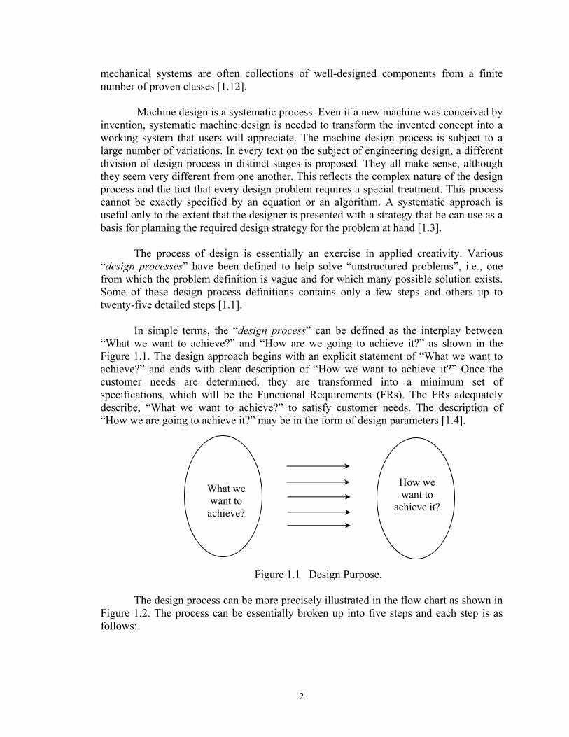
In simple terms, the “design process” can be defined as the interplay between

“What we want to achieve?” and “How are we going to achieve it?” as shown in the Figure 1.1. The design approach begins with an explicit statement of “What we want to achieve?” and ends with clear description of “How we want to achieve it?” Once the customer needs are determined, they are transformed into a minimum set of specifications, which will be the Functional Requirements (FRs). The FRs adequately describe, “What we want to achieve?” to satisfy customer needs. The description of “How we are going to achieve it?” may be in the form of design parameters [1.4].

How we want to

achieve it?

What we want to

achieve?

Figure 1.1 Design Purpose.

The design process can be more precisely illustrated in the flow chart as shown in Figure 1.2. The process can be essentially broken up into five steps and each step is as follows:

2

1. Pre-design Process. Sometimes, but not always, design begins when an engineer recognizes a need and decides to do something about it. Recognition of the need and phrasing the need often constitute a highly creative act, because the need may be only a vague discontent, a feeling of uneasiness, or a sensing that something is not right. The need is often not evident at all; recognition is usually triggered by a particular adverse circumstance or a set of random circumstances, which arise almost simultaneously. For example, the need to do something about a food-packaging machine may be indicated by the noise level, by the variation in package weight, and by slight but perceptible variations in the quality of the packaging or wrap. It is then followed by the definition of the problem. Definition of the problem must include all the specifications for the things to be designed. The specifications are the input and output quantities, the characteristics and dimensions of the space the thing must occupy, and all limitations on these quantities. We can regard the thing to be designed as something in a black box. In this case we must specify the inputs and outputs of the box, together with their characteristics and limitations. The specifications define the cost, the number to be manufactured the expected life, the range, the operating temperature and the reliability [1.13]. The problem definition also consists of the constraints, such as e.g. environmental constraints, dimensional constraints etc.

2. Synthesis and Analysis. The synthesis scheme connecting possible systems

elements is sometimes called the invention of the concept. This is the first step in the synthesis task. In Synthesis as many alternative designs are sought, usually without regards (at this stage) for their value and quality [1.13]. This is also referred to as ideation and invention step in which as many creative solutions as possible are generated. Here creativity plays an important role. In the next step, analysis must be performed to assess whether the system performance is satisfactory or better and, if satisfactory, just how well it will perform. This is an analysis task. System schemes that do not survive analysis are revised, improved, or discarded. Those with potential are optimized to determine the best performance of which the scheme is capable. Competing schemes are compared so that the path leading to the most competitive product can be chosen. Synthesis draws heavily on talent. In this iteration the specification set is formed.

3. Detailed Design and Design Analysis. The intent of the detailed design phase of

the design process is to develop a set of drawings, and geometric models that completely describes the design [1.2]. The proposed design needs to be analyzed and here the analysis techniques come into picture. In the past a stress analysis of individual components was carried out by either using mechanics of materials principles or experimentation [1.3]. The former is inadequate for the analysis of complex shapes, since it is too lengthy and costly. Experimentation requires too much time to make prototype parts and then test them individually. If the part fails then it is redesigned, manufactured and tested again. Finite element analysis plays an important role in this phase. Virtual models can be immediately analyzed for stresses. The process helps in design perfection so that a part may not be rejected in further testing. After the part is designed, it can be analyzed so that its

3

acceptability in that application is determined. The process takes very little time as compared to experimentation and can be used to analyze more complex shapes. We will discuss the use of Finite Element Analysis (FEM) in section 1.5.

4. Prototype Testing. The prototype parts are made from the final design; they are

assembled and tested for various loading conditions, including the durability test. The prototype is tested in actual conditions and its failure mode is predicted. Making the prototype part is the most time consuming part in the entire design process. But, with the advent of tools like Rapid Prototyping has helped the design engineers to make the prototype parts rapidly and try them for assembly. Rapid Prototyping will be more discussed in the section 1.7.

5. Production and Marketing. After the part has passed the testing phase, the

production parts are manufactured. The role of the design engineer does not necessarily end after beginning of the production. This is the most important process in the whole design process as the product is being sold to the customer and the engineer is the one who approves the final design.

Production and Marketing

Prototype / Testing

Is Design OK?

Detailed Design and Design Analysis

Synthesis and Analysis

Pre- Design Process -Recognition of Need -Background Research -Problem Definition

Yes

No

Figure 1.2 Design Process.

4

1.4 Computer-Aided Engineering and Finite Element Analysis The computer has created a true revolution in engineering design and analysis.

Problems whose solution methods have literally been known for centuries but that only a generation ago were practically unsolvable due to their high computational demands can now be solved in minutes on inexpensive microcomputers. One can no longer “do engineering” without using its latest and most powerful tool, the computer.

As the design progresses, the crude freehand sketches made at the earliest stages

will be supplanted by formal drawings made either with conventional drafting equipment or as is increasingly common, with computer-aided design (CAD) and computer-aided drafting software. Present versions of CAD software packages allow (and sometimes require) that the geometry of the parts be encoded in a 3-D database as solid models. In the solid models the edges and the faces of the part are defined. From this 3-D information, the conventional 2-D orthographic views can be automatically generated if desired. Solid modeling systems usually provide an interface to one or more commercial Finite Element Analysis (FEA) programs and allows direct transfer of the model’s geometry to the FEA package for stress, vibration, and heat transfer analyses.

The techniques referred above along with the CAD are a subset of the more

general topic of Computer-Aided Engineering (CAE), which term implies that more than just the geometry of the parts is being dealt with [1.1]. However, the distinction between CAD and CAE continues to blur as more sophisticated software packages become available. In fact, the description of the use of solid modeling CAD system and an FEA package together is an example of CAE. When some analysis of forces, stresses, deflections, or other aspects of the physical behavior of the design is included, with or without the solid geometry aspects, the process is called CAE [1.1].

During the design process, the main concern of a design engineer is the stress

analysis. Although Castingliano’s method computes elastic deflections and forces for more difficult problems, the finite element method will solve problems when the component geometry and loading are complex and cannot be modeled accurately with standard strength of materials techniques. In these complex cases, the determination of stresses, strains, deformations, and loads favors the finite element method, an approach that has broad applicability to different types of analyses (deformations, stress, plasticity, stability, vibration, impact, fracture etc.), as well as to different classes of structures (shells, trusses, frames - and components - gears, bearings, and shafts, for example) [1.5].

In general, the finite element method is based on a theory whereby the body is

viewed as an assembly of discrete building blocks. The application of the method involves dividing the body into an optimum number of blocks (elements) and using them as basis for computations; These blocks are considered severed from each other and joined only at specific points (nodes), forming a network. The number of elements is determined by two factors: the capabilities of the computer being used and the desired accuracy.

5

1.5 Overview of Traditional Finite Element Analysis Traditionally, FEA is one of the most widely used engineering tools to determine

deflection, stress and failure of mechanical parts under service loads. FEA can be thought of as an approximation technique for analyzing complex structures which, handled as a whole, would represent a mathematical model much too complicated to set up and solve. Instead, FEA uses a three-step approximation technique to tackle manageable pieces of the problem, and then combine the results into an overall solution. In the first step, called Pre-processing, a mathematical model is constructed by dividing the structure into elements connected at nodes to form mesh. Next, the solver performs the numerical analysis on a computer to determine the behavior of structure. This is referred as the Processing phase. In the last step, called Post-processing, the computer converts the analysis results from raw number into graphical form of display [1.7].

Earlier, FEA was used mainly a research tool, but was seldom used in daily

engineering practice. It found acceptance primarily in the research center of large corporations, particularly in the aerospace industry. There, large, complex structures such as airplanes were analyzed to verify design performance [1.8].

In a workshop, a panel of leading users discussed the problem of computer-aided

engineering (CAE) in the design cycle. Their consensus was that, due to time limitations, and lack of confidence in the results, FEA was not being used in the early stage of the design phase where it would be most beneficial. A similar situation exists in Japan: in a state-of-art report on Japanese Computer-Aided-Design (CAD) methodologies for mechanical products Whitney states, “Everyone I visit says it takes too long to prepare data for FEA. Even those who have ‘automatic meshers’ say so.”[1.9].

1.6 Current Status of FEA in Design Process

The design of machine part may be done in two different ways – either choosing a

standard form and material that fits the requirements; or creating a new form, that is, planning the geometry and choosing the materials to fit the requirements. The first alternative is called the direct, or check problem, and the second alternative is called the inverse, or design problem. For simple parts, both check and design problems can be solved relatively easily using available strength formulas. With complex machine parts, seeking a solution is a more difficult process as the geometric variables become too numerous and stress computation becomes mathematically indeterminate. The design problem approach is therefore different from the direct problem [1.6].

Design is an iterative process of improvement. It starts with a certain assumption

of the geometric form, dimensions, and materials. Through the computational process, arrives at a solution, finding the distribution and the magnitude of stresses, thus identifying the weakest spot for design changes. And then improves the assumption of form, dimensions and materials, and repeat the solution step-by-step until a satisfactory design is obtained. At times, the design may require several iterations involving geometry changes with repeated analyses. At other times, the first analysis is sufficient. Again, the

6

designer may use the same geometric form and simply revise the design by changing material [1.6].

As FEA began to enter in daily engineering activities, its scope was limited as far

as the design is concerned. Analysis was done by the dedicated analyst with the knowledge and experience to properly apply the technology. Traditionally, engineers designs parts independently and then throw them “over the wall” to analyst, who assigns a priority to the project and then performs a stress analysis when they can. Engineers may provide CAD models from which analyst can build the FEA model. But in many cases, part geometry is conveyed as two-dimensional that must be interpreted and translated by the analyst. It may take days or even weeks before the analysis is completed [1.9].

In most organizations, this exchange is so inefficient that FEA typically is applied

only in the final design phases. Often it happens that the part fails in the prototype-testing phase. The designer then redesigns the part and sends it back though testing analysis cycle. The design-test-redesign cycle adds considerable time and expense to the product development cycle. 1.7 Rapid Product Development Process

Three enabling technologies have emerged to provide the communication,

visualization, and simulation capabilities required by Rapid Product Development (RPD). These technologies are 3D solid modeling, FEA, and rapid prototyping [1.14].

Solid models of the parts and assemblies, as discussed earlier, have allowed

designers to quickly represent their ideas in an ambiguous manner (visualization and communication). Team members can qualify assembly techniques, manufacturability, and “look and feel” (simulation).

Rapid prototyping has bridged the virtual and physical worlds. The technology has progressed to the point where an engineer can literally make a “3-D print” of part in matter of hours. Engineering and marketing can test subtle variations of a concept and incorporate suggestions into prototypes in near “real time” (simulation). While the solid model can convey much data about a part using shaded, dynamic, on-screen manipulation, it is very difficult to pass a monitor and mouse around to meeting participants. In contrast, a physical part can answer many questions.

Although, the resultant deformations calculated by an analysis can often shed

light on form and fit, FEA focuses on the function part of the form-fit-function equation. Understanding stress levels, deformation, temperatures, and response to vibration or fluid flow characteristics up-front in the design process is clearly the embodiment of simulation. Multiple design iterations on conceptual geometry can easily lead to a radical new design or a significant reduction in the number of prototypes. Today’s analysis tools also greatly enhance an engineer’s ability to visualize and communicate with rendered and animated color contour plots of parts under test.

7

Most engineers also have recognized the value of RPD and the importance of all the enabling technologies contributing to that process. However corporations have accepted these technologies to varying degrees. It is interesting to note that the acceptance of these technologies is not proportional to their maturity. The illustration in Figure 1.3 shows the relative age and acceptance level in product design of the core tools. Solid modeling tools were invented in mid 80s and it is used in 90% of the industries. Rapid prototyping concept was also invented in mid 80s and its use is 60%. But though invented in mid 60s and its use is in only 30 %.

Figure 1.3 Relative acceptance and age of three enabling technologies [1.14]. The different level of acceptance of these tools sheds light on the reluctance of

traditional design organizations to break away from familiar processes. Drawings and prototypes have been the mainstay of design groups throughout history while actual engineering has often been a small part of the overall process. In traditional product design process used at most companies, increasingly shorter time lines preclude lengthy engineering evaluations of the performance of chosen configurations. Even today, many engineering companies would prefer to take the chance that a “best guess” design will work, thereby risking possible redesign. This seems more attractive due to that instant gratification alluded to earlier than delaying the creation of initial prototypes through expanding early analysis in order to reduce testing and prototyping. Figure 1.4 depicts the traditional product design process used at most companies.

8

Figure 1.4 Traditional product development process [1.14]. Conceptual designs are rushed through the system. Here, the primary task of engineering is to develop layouts and drawings. When structural functionality is clearly an issue up-front, it may be addressed by calculations, analysis, or over-design during the drawing creation stage. The true performance of a part or system is typically not understood until the prototyping and testing phase. If no issue arises during these phases, the design is often deemed acceptable and considered finished. If time and budget permit, some degree of optimization is performed on a trial and error basis until schedule and costs dictate the end. If the part fails the testing phase, companies typically scramble to resolve the problem with as little change as possible. FEA is often brought in at this stage. However, the engineer’s hands are somewhat tied by the design envelope dictated by other released and in-process components. True optimization is very difficult at this stage. And the changes required may not be the most cost effective due to these restrictions. Figure 1.5 indicates the relative cost and the difficulty in design changes at various stages of the design phases. The longer it takes to make these changes the more difficult it is to make modification and costs significantly increase [1.14].

9

Product Development

Diff

icul

ty a

nd C

ost I

nvol

ved

In D

esig

n C

hang

es

Concept Design Prototype Pilot-Production Production Installation Market

Design ProcessFigure 1.2

Figure 1.5 Difficulties and cost in design changes [1.11].

One of the reasons for the relative cost of change later in the process can be better understood by studying Figure 1.6, which indicates the disparity of a company’s investment in a design compared to their level of understanding. The “build and break” cycle controls the area between the curves in Figure 1.6. The more cycles required, the greater the gap in knowledge versus cost. In fact, experienced manufacturers from different industries have shown that 90% of the project cost is determined at the initial stage of the design, where 10% of the total cost of the project is spent [1.1].

Figure 1.6 Cost spent versus product knowledge [1.14].

10

It should be clear that the value of the early analysis lies in the reduction of

knowledge gap and in the potential for saving in later stages of the product development cycle. The next Figure (Figure 1.7) shows the ideal predictive engineering enabled design process where the test / redesign cycle is performed on software prototypes. Not only can planned testing then be done more quickly and with less cost, simulation can allow the engineer to explore design options or loading scenarios, which would be too costly to address in physical world. The revised design process results in rapid closure of the knowledge graph of the disparity between investment and understanding as shown in the Figure 1.8.

Figure 1.7 Product Development using early analysis [1.14].

Figure 1.8 Improved Cost spent versus product knowledge with Early Analysis [1.14].

11

1.8 Early Analysis: The New Engineering Paradigm Clearly, if analysis can be carried out earlier in the design process, the benefits

will be significant, including shortened time to market, improved product design and reduced product development cost. The way to accomplish this is by re-orienting the process itself so that the analysis is performed much earlier in product development. This moves CAE forward into the conceptual phase. This step involves synthesis and analysis (Phase 2 in Figure 1.2), where changes are much easier and more economical to correct a poor design.

A major benefit of early analysis is the ability to perform a “what-if?” simulation.

This helps the designer to consider and evaluate alternate approaches and to explore options in the early design cycle. Through this process, engineers and designers can quickly investigate many design variations and evaluate numerous ideas that would not be practical to test in hardware. Moreover, the computer analysis helps them find troubled spots that otherwise will be extremely difficult to isolate in the mess of complex interrelated variables. Also, “what-if?” studies can show engineer the effect of making a design modification to correct a problem in an isolated area, so that such changes do not adversely affect overall product performance [1.10].

Since more resources are focused in the initial design stages, costs during this phase will be higher than the traditional approach. Also design may take somewhat longer to release as concepts are being virtually proven upfront rather than later by repetitive and expensive testing. However this added time and cost is offset later through savings in prototype testing and fewer engineering changes.

In short, the use of analysis in the early design phases design phase supports the

compression of the product develop cycle by changing the manner in which errors are found and the design is refined. Earlier without CAE, the design to get finalized it has to be gone through the repetitive stages of design, prototyping and testing. But now there is no need of this repetitive process when using CAE. This is summarized in Figure 1.9. In using analysis in early design phases, Computer Aided Design (CAD) and FEM are jointly conducted in the initial stages of the Product Development Cycle. As soon as a CAD model is configured, a preliminary FE analysis is run and the CAD model modified and reanalyzed until it performs optimally. Ideally, the resulting prototype design passes all qualifying tests the first time [1.10].

12

Figure 1.9 Product Development Cycle [1.10].

1.9 Goal and Objectives

The goal of this work is to develop a methodology to carry out finite element analysis in the early design stage to achieve the advantage of introducing early-analysis in the product development cycle. The approach is evolutionary in the sense that the design is evolving, being guided by the analyst and the analyst is responding at every stage during the evolution of the design. The four objectives of this work are as follows:

1. Instantaneous Stress and Displacement Results. This work will enable an engineer to

obtain instantaneous stress and displacement information following a design change in a mechanical component. An engineer can first input an initial design of a component and then carry out a complete finite element analysis, i.e. pre-processing, processing and post-processing. If after post-processing it is felt that the stresses/displacements are too large, s/he can modify the component geometry graphically and the system will generate the results for the changed geometry based on the displacement results of the initial design (mesh). The work will allow an engineer to model a mechanical component using the commercial finite element code ANSYS 5.7, and will update the stress and displacement results with each geometric change. The process will continue until the engineer feels that the design is acceptable based on strength and stiffness requirements.

2. Enhanced Computational Performance. Various techniques were used to improve the

computational performance; with the aim of producing results of acceptable accuracy in shorter period of time in order to emphasize the interactive nature of the design process. In this way a design may be optimized, though not in a mathematical sense. Instead, the optimization uses the experience of the engineer, who is very much aware of the possible effects of design changes on stress and displacement results.

13

Techniques of re-analysis for structural optimization will be used in this work. Significant research on re-analysis has been done from the early 60s until recently [1.15, 1.16].

3. User Friendly. The system will be developed using the commercial finite element

code ANSYS 5.7. The reason why ANSYS is used is that its customizable features allow easy development of the system. Furthermore, the user-friendly features will help an engineer to carry out an analysis and reanalysis more easily.

This work is original and can be termed as evolutionary because it modifies the old trend and methodology of design process. Also the techniques used in this work to improve the computational effort such as, combined approximation reanalysis, were first developed only for structural optimization. During structural optimization the problem under consideration is repeatedly analyzed to assess changes in behavior due to geometric and structural modifications of the part. However, this method has never been applied to complex finite element types, though the concept is the same. 1.10 Significance of Work

The major beneficiaries of the work will be engineers working in product development and validation of components and structures, which are subjected to mechanical loads. It has long been accepted that the conceptual stage of mechanical product design development is of prime importance. It is at this stage that the fundamental geometry of a design is set, and as the evolution process continues it becomes significantly more expensive, more technically and organizationally challenging, to bring about a radical change to the design laid out at the conceptual stage. Conventional Finite Element software packages have also been found to have limited use to an engineer in the early design stage. The analysis model defined in a commercial software package is contrary to the idea process of conceptual design evolution since it forces the numerical model to be a detailed design. Furthermore, it is also well known that modifications to analysis models can become time-consuming even for simple geometric perturbations.

The scientific and technological relevance of this work applies not only to the

early stage of design, but to a number of other applications areas in which benefits may accrue. A company may have needs for a rapid analysis and re-analysis tool to carry out fatigue assessment of components manufactured slightly out of tolerance. Typically this needs to be carried out under a very restrictive time scale. Furthermore, although the approach described here represents an engineer-driven optimization, it is clear that a rapid re-analysis solution would be valuable in a mathematical optimization procedure. Whether sensitivity information, hill climbing, or some more sophisticated scheme drives the optimization, it is clear that a stress analysis would often be performed on a model slightly perturbed from previous design iteration. Therefore, a solution of the type described in this work would have widespread relevance.

14

2. Structural Reanalysis 2.1 Design Optimization The design process is divided in five distinct steps (shown in Figure 1.2) as discussed in the Section 1.3. The second step in the process is the Synthesis and Analysis. During the pre-design process within a selected concept there may be many possible designs that satisfy the functional requirements, and a “trial-and-error” procedure may be employed to choose the optimal design. Selection of best geometry or the cross-sections of the member are examples of the optimal design procedure. The procedure is referred to as the optimization process. Thus, optimization in the present context is an automated design procedure giving the optimal design values of certain design quantities, considering desired criteria and constraints. 2.2 Design Variables A structural system can be described by a set of quantities, some of which are viewed as variables during the design optimization process. Those quantities defining a structural system that are fixed during the automated design are called pre-assigned parameters and they are not varied by the optimization algorithm. Those quantities that are not pre-assigned are called design variables. The pre-assigned parameters, together with the design variables, will completely describe a design. From a physical point of view, the design variables that are varied by the optimization procedure may represent the following structural properties [2.1]: 1. The mechanical and physical properties of the material. 2. The topography of the structure, i.e., the pattern of connection of the members or

the number of the elements in the structure. 3. The configuration or the geometric layout of the structure. 4. The cross-sectional dimensions or member sizes.

Even though the properties described above are related to the Structural

Optimization, they are more or less related to the properties in finite element analysis. In this work to be presented we will address the third property i.e. the geometric layout of the structure in context to finite element analysis. In structural system this property means the structural layout of the truss members to achieve certain support conditions. In finite element it means the nodal coordinates and element shapes. 2.3 Structural Reanalysis Since design is an iterative process, the introduction of analysis in the design process, demands repetitive analysis of the design concepts. Typically a sequence of design and redesign is carried out until certain features such as weight, natural frequency, mode shape or stress magnitudes attain suitable values [2.2]. Therefore, the design optimization process becomes iterative and requires repeated analysis of structures obtained by progressive modification in design variable [2.3]. This operation, which

15

involves much computation effort, is one of the major obstacles when applying optimization methods to large systems. Because of the large number of analysis required, it very important to develop efficient reanalysis techniques, especially for structures analyzed by finite element method, for only a small number of elements that are modified at each design step [2.4]. Reanalysis methods are intended to analyze efficiently modifications in a design using information from the previous design [2.3].

The definition of the structural static reanalysis is stated as follows: Find the response under the static load of a structure after modifications using the original response of the structure such that the computational time of reanalysis is less than the complete analysis time [2.4]. At the same time, reanalysis techniques allow one to efficiently compute the design sensitivity coefficients required for optimization methods. Reanalysis techniques are particularly important for large structures, especially in finite element analysis where only a small part of the structure / mesh is progressively modified. Such reanalysis techniques may be easily implemented in computer codes with minimal difficulty [2.6].

The finite element method in general requires the solution of the set of linear equilibrium equations,

(2.1)00uKF =

where, is the mesh stiffness matrix, is the column vector of unknown nodal displacements, and is the column vector of externally applied loads. Consider a design problem in which the design variables represent only the geometry of the structure and the loadings are fixed. The elements of are the functions of the design variables, and the elements of are assumed to be fixed.

0K 0uF

0KF

This chapter deals with different types of reanalysis methods in which changes are made in the design variables. As a result, we have corresponding change in the stiffness matrix K∆ and in the displacement vector u∆ . The objective is to find new displacement vector u .

uuu ∆+= 0 corresponding to new stiffness matrix K .

KKK ∆+= 0 One possibility is to analyze the new design by solving the new set of equations

KuF = this might be the best way in some cases where large modifications are made to a large part of the structure. However, in many cases when either a relatively small proportion of the structure is modified, or minor modifications are made to a large part of the structure, reanalysis methods might prove to be more efficient. Instead of performing a complete new analysis of the modified design by solving equations from a force-displacement relationship, it is often advantageous to use known values of u from the previous analyses.

0

(2.2)

No single method of reanalysis is superior in all cases. To solve a particular problem, a method should be selected which is easy to apply and which requires a

16

relatively small computational effort. Furthermore, it might be sometimes more efficient to employ a combined technique which based on more than a single method.

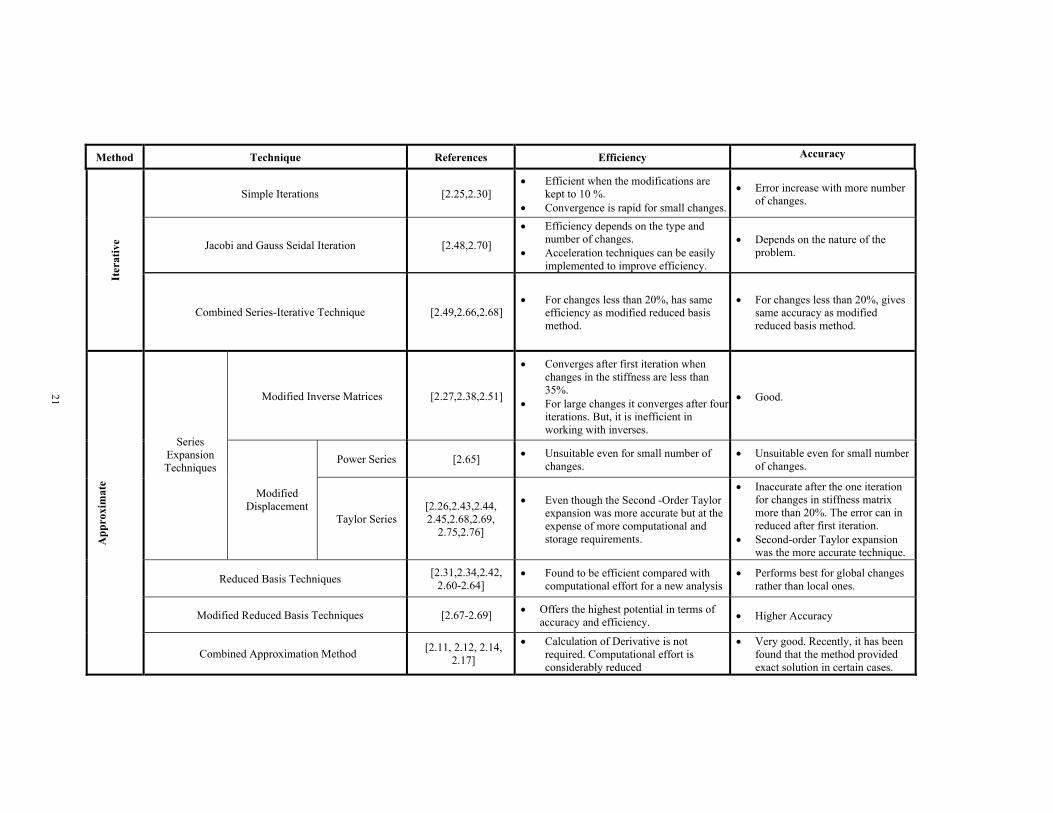
Reanalysis techniques may be broadly classified as, 1. Direct (Exact) 2. Iterative 3. Approximate These methods will now be discussed and are shown in Table 2.1.

Direct (Exact) methods are most efficient if the number of modified elements in

the stiffness matrix is limited. This is the case, for example, if the coordinates of very small number of nodes are changed. The incremental stiffness matrix K∆ in this case could be compressed, by eliminating zero columns and rows, to form a reduced incremental matrix of size equal to the number of changed columns (or rows) in matrix . The relation between

RK∆

0K K∆ and RK∆ is given by, bKbK R

T ∆=∆ where is a Boolean matrix with linearly independent rows, each of which contains all zeros except for one unit value, located at the column numbers where the change in occurs. For example, if

b0K

K∆ is given by,

∆∆∆∆∆

∆∆

=∆

000000000000000000

3332

232221

1211

KKKKK

KK

K

we define matrix b by,

=

001000001000001

b

and the reduced matrix, is, RK∆

∆∆∆∆∆

∆∆=∆

3332

232221

1211

0

0

KKKKK

KKK R

One direct method to reanalyze the structure is to compute the inverse of the modified stiffness matrix 1−K , using the known inverse of the original matrix. This algorithm is based on Sherman-Morrison identity [2.5] which can be written for the incremental matrix or, alternatively, for its single elements or columns. There are many Direct RK∆

17

Methods which can be used for reanalysis. Table 2.1 gives different types of the direct methods.

We can observe from the above illustration, Direct Method gives exact, closed-

form solution that has the same effect of solving the modified system of equations from beginning without using any reanalysis technique. In general, direct methods are efficient if the number of modified elements is small, because for larger number of changes, the calculations become so high that solving the system with direct method becomes inefficient.

Iterative methods for reanalysis might be more suitable for minor modifications to a large part of a structure [2.1]. These methods apply successive correction to the initial solution and may converge to the most accurate solution for the modified structure. In these methods solution accuracy and rate of convergence are important. In iterative methods of reanalysis, the displacement vector u can be used as an initial solution for the iteration process [2.1]. One inherent drawback of these methods is that the entire process must be repeated for each loading condition. However, in view of the fact that stiffness matrices are banded and may possess a large number of zeros even within the band, an iterative scheme using only the nonzero elements of K and K∆ is advantageous from a storage point of view and may require less algebraic operations. One major difficulty which might be encountered during solution is concerned with convergence which is not always ensured, or might be slow. Computational effort and efficiency has to offset accuracy. These two factors can rarely be satisfied simultaneously, because to get near exact solution, the efficiency decreases and vice versa. Therefore some compromise must be made such that “run-time” is not excessive and that solution accuracy is sufficient [2.6].

For simple iteration techniques the force displacement relationship for the

changed finite element model can be written as,

(2.2) FuKK =∆+ )( 0 or

(2.3) )1()(0

−∆−= kk KuFuK where, is the value of u after the k)(ku th iteration, and u is the initial vector known from initial analysis.

)0(

0)0( uu =

Equation (2.3) represents simple iteration, similar to conventional matrix iterative methods for solving linear systems. For solving the equations, if Choleski decomposition is used, then only one triagularization of is needed for any specific modification. Successive cycles of iterations then require only forward and back substitution. Various iterative methods for reanalysis, such as, Jacobi, Gauss-Seidal etc. their efficiency and accuracy are listed in Table 2.1.

0K

18

Approximate methods are generally sufficient to be employed for intermediate designs, which require less computational efforts. While approximate algorithms might be most efficient in many cases, the basic difficulty is usually associated with solution accuracy. Approximate methods are most efficient than direct (exact) methods, and are usually suitable for moderate changes in the whole structure. In general, the calculation efficiency and solution quality are conflicting factors that should be considered. Improved solution accuracy is often achieved at the expense of increased computational effort. Approximate methods can be divided into the following three classes (the details of which are given in Table 2.1):

(a) Global Approximations. Global approximations are also called multipoint and are

based on polynomial fitting or reduced basis methods [2.7-2.9]. These approximations are obtained by analyzing the structure at a number of design points, and they are valid for whole design space (or at least large portions of it). However, Global Approximations may require significant computational effort in problems with a large number of design modifications.

(b) Local Approximations. Local approximations are also called single point

approximations and are based on first order Taylor series expansion or binomial series expansion about a given design point. In other words Local approximations are based on information calculated at a single point. These methods are most efficient, but they are effective only in the case of small changes in design variables. For large changes in design, accuracy of approximations often deteriorates and they may become meaningless. That is, the approximations are valid only in vicinity of a design point. A possibility to improve the quality of the results is to consider second-order approximations [2.10], but this might increase considerably the computational effort.

(c) Combined Approximations (CA). Combined approximations attempts to give

global qualities to local approximations. Similar to local approximations, the calculations are based on results of single exact analysis. Each subsequent reanalysis involves the solution of only a small system of equations. Thus, the computational effort is significantly reduced. Calculations of derivatives are not required, and the method can be used with general finite element program. Recently, it has been found that this method provides exact solution in certain cases [2.11 - 2.13]. This is reason why the method is used for this work.

The next section describes the Combined Approximation Method in-depth and shows the cost analysis of the method.

19

Table 2.1 Comparison of Static Reanalysis Techniques [2.6]

Method Technique References Efficiency Accuracy

Parallel Element Technique [2.73, 2.74] • Very Efficient for a large number of

modifications. • More Efficient than Initial Strain.

• Accuracy is not affected by the magnitude of modifications.

Initial Strain/Stress [2.20, 2.22] • Found Inefficient when compared with the fresh analysis [2.86, 2.87]. • Good.

Mathematical Approach [2.24,2.33,2.35, 2.36,2.83] Modified

Decomposed Matrices Structural Analysis [2.32,2.50,2.53,

2.54,2.71, 2.84]

• Efficient only when the number of modifications is at minimum level. • Good.

Mathematical Approach [2.37,2.39,2.40, 2.41,2.21,2.52,

2.55,2.85] Modified Inverse of Matrices

Modified Inverse of [K] [2.46,2.47,2.65, 2.72]

• Found to be efficient in comparison with Gauss Elimination when the modifications were are small.

• But overall found to be expensive in comparison with the other methods.

• Good.

Modified Displacement Vector [2.21,2.23,2.46,2.47,2.79-2.82]

• More efficient than the Modified Inverse method.

• Expensive in comparison with the complete reanalysis except for small modifications.

• Good.

Linear Combination [2.60-2.64]

Dir

ect

Superposition Technique

Direct Superposition, Theorems of Structural and Geometric

Variation

[2.29,2.56-2.59, 2.77,2.78]

• Inefficient than the method of complete reanalysis. • Good.

20

21

Simple Iterations [2.25,2.30] • Efficient when the modifications are

kept to 10 %. • Convergence is rapid for small changes.

• Error increase with more number of changes.

Jacobi and Gauss Seidal Iteration [2.48,2.70]

• Efficiency depends on the type and number of changes.

• Acceleration techniques can be easily implemented to improve efficiency.

• Depends on the nature of the problem.

Iter

ativ

e

Combined Series-Iterative Technique [2.49,2.66,2.68] • For changes less than 20%, has same

efficiency as modified reduced basis method.

• For changes less than 20%, gives same accuracy as modified reduced basis method.

Modified Inverse Matrices [2.27,2.38,2.51]

• Converges after first iteration when changes in the stiffness are less than 35%.

• For large changes it converges after four iterations. But, it is inefficient in working with inverses.

• Good.

Power Series [2.65] • Unsuitable even for small number of changes.

• Unsuitable even for small number of changes.

Series Expansion Techniques

Modified Displacement

Taylor Series [2.26,2.43,2.44, 2.45,2.68,2.69,

2.75,2.76]

• Even though the Second -Order Taylor expansion was more accurate but at the expense of more computational and storage requirements.

• Inaccurate after the one iteration for changes in stiffness matrix more than 20%. The error can in reduced after first iteration.

• Second-order Taylor expansion was the more accurate technique.

Reduced Basis Techniques [2.31,2.34,2.42, 2.60-2.64]

• Found to be efficient compared with computational effort for a new analysis

• Performs best for global changes rather than local ones.

Modified Reduced Basis Techniques [2.67-2.69] • Offers the highest potential in terms of accuracy and efficiency. • Higher Accuracy

App

roxi

mat

e

Combined Approximation Method [2.11, 2.12, 2.14, 2.17]

• Calculation of Derivative is not required. Computational effort is considerably reduced

• Very good. Recently, it has been found that the method provided exact solution in certain cases.

Method Technique References Efficiency Accuracy

21

2.4 Combined Approximations (CA) Method and its Cost Analysis We have seen in the previous section that, for the Combined Approximation method the calculations that are based on results of a single exact analysis. Because of reduced computation effort, the method can be applied to a general finite element program. Several studies in early eighties have shown [2.14] that combined approximations can be introduced by scaling the initial stiffness matrix such that the changes related to the scaled design are reduced. The advantage of this approach is that the solution is based on results of a single exact analysis. It has been demonstrated that the scaling procedure is useful for various types of design variables and behavior functions. Several criteria for selecting the scaling multiplier have been proposed, based on geometrical and mathematical considerations [2.13]. In early nineties, it has been found [2.15, 2.16] that scaling both the designs and the modified approximate displacements can be expressed in reduced basis form. Extending the concept of scaling to include also the approximate displacements significantly improved the results. It has been shown also that high quality approximations can be achieved for very large changes in the design variables by considering only two basis vectors. 2.4.1 Problem Formulation The reanalysis problem considered for this study can be stated as follows [2.14]:

a) We start with given initial design. For FEA we construct a mesh and find corresponding square stiffness matrix , and the column vector for nodal forces

, the corresponding displacement column vector u are computed by solving the force-displacement relationship of the mesh:

0KF 0

00uKF = (2.4)

It is assumed the mesh stiffness matrix is given from the initial analysis in the decomposed form:

0K

000 UUK T= (2.5)

where U is upper triangular matrix. 0

b) Assume changes in the geometry (coordinates of nodes) so that the modified

square stiffness matrix K is given by

KKK ∆+= 0 (2.6) where K∆ is the change in the stiffness, due to changes in the geometry.

22

c) The goal is to find efficient and accurate approximations of the modified displacements due to various changes in the geometry, without solving the complete set of modified analysis equations.

u

FuKKKu =∆+= )( 0 (2.7)

Once the displacements are evaluated, the explicit stress-displacement relations can be used to determine the stresses. Thus, the presented approximations of are intended only to replace the set of implicit analysis Equation (2.7).

uu

The above formulation is general and can be applied to different types of design variables and structures. For illustrative purposes, discrete structures are considered in this study, but the approach presented is suitable for the shape changes in continuum structures. 2.4.2 Combined Approximation Reanalysis In Combined Approximation Reanalysis (CA), the computed terms of the binomial series expansion are used as high quality basis vectors in reduced basis approximations. The unknown coefficients of the reduced basis expression are determined by solving a reduced set of analysis equations. For completeness of presentation, evaluation of the displacements by the combined approximation method is briefly described in this section. Given the initial stiffness matrix in the decomposed form of Equation (2.5), the initial loads and the initial displacements u , calculation of the modified displacements for any assumed changes

0K

0F 0 uK∆ , F∆ , in the stiffness matrix and in the load vector,

respectively involves the following steps:

a) The modified stiffness matrix K and the modified load vector are first introduced. Since and are given, this step involves only introduction of

F0K 0F

K∆ and . F∆ b) The basis vector is calculated. Define square matrix iu B as

KKB ∆= −1

0 (2.8) Pre-multiplying Equation (2.7) by , substituting Equations (2.4) and (2.8) and pre-multiplying the resulting equation by , yields the following expression for the displacements:

10−K

1)( −+ BI

0

1)( uBIu −+= (2.9) For small changes in K∆ , this expression can be approximated by the binomial series,

23

0

12 ),,( uBBBIu s−+−+−= K (2.10) Equation (2.10) in the series of basis vectors, defined as

FKu 101−= (2.11)

1−−= ii Buu (2.12) si ,,2 L=

where is the number of vectors considered (it is assumed that number of degrees of freedom), the matrix of the basis vectors u is defined by

s <<sB

][ 21 sB uuuu K= (2.13)

In the case where , the first basis vector is simply 0=∆F 01 uu = . Calculation of the basis vectors by Equation (2.12) involves only forward and backward substitutions in cases where is available in the form of Equation (2.5) from the initial analysis of the structure. For example, assuming that u is given, the column vector u is calculated by

0K

1

2

120 KuuK ∆−= (2.14)

We solve first for the vector of unknowns t by the forward substitution

10 KutU T ∆−= (2.15) The vector is then calculated by the backward substitution 2u

tuU =20 (2.16) Similarly, is calculated by 3u

230 KuuK ∆−= (2.17)

c) The reduced square matrix and the reduced column vector , are calculated by

RK RF

B

TBR KuuK = (2.18) FuF T

BR =

d) The column vector of unknown coefficients is calculated by solving the set of equations [2.17],

y)( ss ×

24

RR FyK = (2.19)

e) The modified displacements u are evaluated by

Bss uyuyuyuyu ⋅=⋅++⋅+⋅= K2211 (2.20) The flowchart in Figure 2.1 outlines this entire process of the combined approximation reanalysis. Table 2.2 shows the cost analysis of the algorithm used.

25

Solve 10 −∆−= s

T KutU

Solve tuU s =0

][ 21 sB uuuu K=

Solve RR FyK =

BTBR KuuK =

FuF TBR =

yuuyuyuyu Bss =⋅++⋅+⋅= K2211

No need to find explicitly.

K∆ Change in the Geometry

0U Upper Triangular Matrix

0K Initial Stiffness Matrix

0u Initial Nodal Displacements

0F External Nodal Forces

Solve, 000 uKF =

Solve 10 KutU T ∆−=

Solve tuU =20

Solve 20 KutU T ∆−=

Solve tuU =30

KKK ∆+= 0

000 UUK T=

Modified Design

KKB ∆= −10

01 uu =

Initial Design

Figure 2.1 Combined Approximation Reanalysis Flowchart

26

Table 2.2 Combined Approximation Cost Analysis

Step No. Operation Approximate

Multiplications Comments

Initial Design

1 Solve

00uKF =

+ 2

3

6nn [2.18] Solution based on Cholesky

decomposition.

Modified Design

2 Find

KKK −=∆ 0 n (subtractions)

3 01 uu = -

4 1Ku∆− 3m mK

is the number of rows changed in because of change in geometry. 0

5 Solve

10 KutU T ∆−= 2n Forward Substitution.

6 Solve

tuU =20 2n Backward Substitution.

7 2Ku∆− 3m

8 Solve

20 KutU T ∆−= 2n Forward Substitution.

9 Solve

tuU =30 2n Backward Substitution.

M M M Continue till finding u . s

10 ][ 21 sB uuuu K=

- sn × matrix (only m non-zero

terms) 11 KuT

B 2sm ))(( nnns ×× 12 RB

TB KuKu =)( ms 2 )())(( sssnns ×=××

13 FuF TBR = sm )1)(()1( ××=× nnss

14 Solve

RR FyK = 2

3

3ss

+ Based on Gauss elimination with partial pivoting.

15 yuu B= sn Note: Assume the stiffness matrix contains n0K n× terms. For the changed geometry, only elements in the stiffness matrix out of are changed. Generally for good accuracy,

mm ×

0K nn × 3=s so 33× matrix has to be solved [2.19]. 2.5 Comments on Combined Approximation in Finite Element Analysis

The Combined Approximation procedure discussed in Section 2.4 is used in this work for analyzing a plane stress problem using four-node quadrilateral elements. Kirsch [2.3,2.11,2.12,2.14,2.17] introduced the Combined Approximation method by coupling

27

the accuracy of Global Approximation (GA) with the efficiency of Single Point Approximations (SA). This has been mainly used in the past for structural optimization. Very few research efforts have been carried out using CA with more complex element types other than the truss and beam. Gullickson and Averill [2.19] used the CA method to show its use with general finite element procedures. The accuracy and efficiency of CA was demonstrated with a one-dimensional bar element for stress analysis and the two-dimensional four-node quadrilateral element for heat transfer. The authors found that as the number of basis vectors (shown as ‘s’ in Table 2.2) is increased; the CA reanalysis method results converge quickly to the reference solution for all problems tested. The relative number of basis vectors necessary for an accurate approximation decreases as the number of degrees of freedom in the problem increases.

28

3. ANSYS Interface and Supporting Routine 3.1 Introduction The previous chapter discussed the combined approximations (CA) method that is used for reanalysis. In this work CA was integrated into the commercial finite element code ANSYS 5.7. A mechanical component can be developed by creating the two-dimension model in ANSYS using four-node quadrilateral elements. The analysis problem is then solved using the ANSYS solver. If the engineer decides that the stress and displacement results are not acceptable, then ANSYS can be used to change the geometry of the component. The modified problem is solved using the combined approximation reanalysis method in this work. ANSYS was used in this work due to its open architecture since routines and subroutines can be written in C or FORTRAN and either linked to ANSYS or used with external commands. In fact, some of the ANSYS features seen today as “standard” offerings originated as user programmable features (UPFs). The user programmable feature is an ANSYS capability where one can write his/her own routines. Even a design optimization algorithm can be written that calls the entire ANSYS program as a subroutine. UPFs provide the following capabilities [3.1]:

• To read or retrieve information from the ANSYS database. One can create subroutines and either links them to the ANSYS program or use them as external command features.

• ANSYS provides a set of routines that can be used to specify loading types that include body forces, pressures, etc.

In this work the finite element problem is solved using reanalysis methods, the user programmable features and other ANSYS features. UPFs are mainly used to read files generated by ANSYS, details of which are discussed later in this chapter. Although, UPFs allows programming in C and FORTRAN, FORTRAN is used. FORTRAN can interact with ANSYS directly as ANSYS itself uses FORTRAN to solve finite element problem. Many readymade FORTRAN subroutines are provided by ANSYS to obtain information from the database. Using C requires a converter to access those subroutines as functions in C. 3.2 ANSYS Interface ANSYS 5.7 is used to develop the platform for solving the reanalysis problem. Before discussing details of the development platform, some ANSYS basics and its GUI will be first discussed. 3.2.1 ANSYS Program Organization Before introducing the Graphical User Interface (GUI), some basic concepts of ANSYS program will be discussed. The ANSYS program is organized into two levels:

29

1) the BEGIN Level and (2) the PROCESSOR Level. Upon first entering the program, the user starts in the BEGIN level and can then enter the ANSYS processors shown in Figure 3.1.

Enter ANSYS Exit ANSYS

BEGIN LEVEL

PREP7 POST1 POST26 Etc. SOLUTION General General Time-History

Processor Preprocessor Postprocessor Postprocessor

PROCESSOR LEVEL

Figure 3.1 Organization of ANSYS 5.7 [3.2].

One may have more or fewer processors available than those shown in Figure 3.1. The actual processors available depend on the particular ANSYS product you have. The Begin level acts as a gateway into and out of ANSYS. It is also used to access certain global program controls. At the PROCESSOR level, several routines (processors) are available; each accomplishes a specific task. Most analyses will be done at the PROCESSOR level. A typical analysis in ANSYS involves the following three steps [3.2]:

1. Preprocessing. The PREP7 processor is where the user defines geometric, materials, and element types to ANSYS.

2. Solution. The SOLUTION processor is used to define the analysis type, set boundary conditions, apply loads, and initiate the finite element solution.

3. Postprocessing. POST1 (for static or steady-state problems) or POST26 (for transient problems), can be used to review the analysis results in the graphical user interface and tabular listings.

Only PREP7, SOLUTION and POST1 processors will be used in this work since static stress analysis considered. These processors are denoted by the shaded boxes in Figure 3.1. The next section presents a brief overview of the Graphical User Interface.

3.2.2 Graphical User Interface The simplest way to communicate with ANSYS is by using the ANSYS menu system, called the Graphical User Interface (GUI). The GUI provides an interface

30

between the user and ANSYS. The program is internally driven by ANSYS commands. However, by using the GUI, an analysis with little or no knowledge of ANSYS commands can be performed. This process works because each GUI function ultimately produces one or more ANSYS commands that are automatically executed by the program. The ANSYS GUI consists of the following six main regions [3.3] as shown in Figure 3.2:

Utility Menu. This menu contains utility functions that are available throughout the ANSYS session, such as file controls, selecting and graphic controls. One can exit ANSYS through this menu.

Main Menu. This menu contains the primary ANSYS functions organized by processors. These functions include preprocessor, solution, general postprocessor, design optimizer, etc.

A

B

A

CD

B

E

F

Figure 3.2 Regions of the ANSYS 5.7 Graphical User Interface

31

Toolbar. The toolbar contains push buttons that execute commonly used ANSYS commands and functions. The user can add his/her own pushbuttons by defining abbreviations.

Input Window. The input window displays program prompt messages and allows one to type in commands directly. All previously typed-in commands also appear in this window for easy reference and access.

Graphics Window. The graphic window is where graphics displays are drawn.

Output Window. This window receives text output from the program. It is usually positioned behind the other windows.

C

D

E

F

The User Interface Design Language (UIDL) can be used to modify the Main Menu. Furthermore, user specific Menu Items can be added by using the UIDL. UIDL and how it was used in this work will be discussed later in Appendix D. Furthermore, ANSYS customization features allow changing the Toolbar as per the user’s requirements. 3.2.3 ANSYS Database and Files The previous section explained how ANSYS is organized. This section discusses the ANSYS database and how ANSYS reads and writes various file types during a typical analysis. The information the user inputs when modeling a problem, e.g., element type, material property, dimensions, geometry, etc. is stored as input data. During the solution phase ANSYS computes various results, such as displacements, stresses, etc. and this information is stored as results data. The input data and results data are stored in the ANSYS database. The database can be accessed from anywhere in the ANSYS program. The database resides in memory (RAM of the computer) until the user saves the database to a database file Jobname.DB, where Jobname is the file name. The input and output files that ANSYS reads and writes, respectively, are of the form Jobname.Ext, where the default jobname is file. Files used in this work include the following [3.5]:

• Log File (Jobname.LOG). This file is opened when ANSYS is first entered. Every command issued in ANSYS is copied to a log file. This is very helpful when creating the APDL code for processes which need to be repeated.

• Database File (Jobname.DB). This file is one of the most important ANSYS files because it contains all input data and some results. This is a file where the ANSYS analysis model is stored.

• Output File (Jobname.OUT). This file is opened when the user first enters ANSYS. This file saves responses given by ANSYS to every command executed by the user. It also records warning and error messages and some results.

32

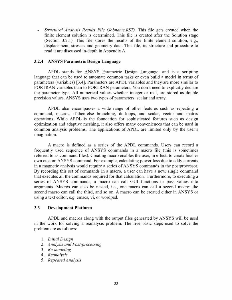
• Structural Analysis Results File (Jobname.RST). This file gets created when the finite element solution is determined. This file is created after the Solution stage (Section 3.2.1). This file stores the results of the finite element solution, e.g., displacement, stresses and geometry data. This file, its structure and procedure to read it are discussed in-depth in Appendix A.

3.2.4 ANSYS Parametric Design Language APDL stands for ANSYS Parametric Design Language, and is a scripting language that can be used to automate common tasks or even build a model in terms of parameters (variables) [3.4]. Parameters are APDL variables and they are more similar to FORTRAN variables than to FORTRAN parameters. You don’t need to explicitly declare the parameter type. All numerical values whether integer or real, are stored as double precision values. ANSYS uses two types of parameters: scalar and array. APDL also encompasses a wide range of other features such as repeating a command, macros, if-then-else branching, do-loops, and scalar, vector and matrix operations. While APDL is the foundation for sophisticated features such as design optimization and adaptive meshing, it also offers many conveniences that can be used in common analysis problems. The applications of APDL are limited only by the user’s imagination. A macro is defined as a series of the APDL commands. Users can record a frequently used sequence of ANSYS commands in a macro file (this is sometimes referred to as command files). Creating macro enables the user, in effect, to create his/her own custom ANSYS command. For example, calculating power loss due to eddy currents in a magnetic analysis would require a series of ANSYS commands in the postprocessor. By recording this set of commands in a macro, a user can have a new, single command that executes all the commands required for that calculation. Furthermore, to executing a series of ANSYS commands, a macro can call GUI functions or pass values into arguments. Macros can also be nested, i.e., one macro can call a second macro; the second macro can call the third, and so on. A macro can be created either in ANSYS or using a text editor, e.g. emacs, vi, or wordpad. 3.3 Development Platform APDL and macros along with the output files generated by ANSYS will be used in the work for solving a reanalysis problem. The five basic steps used to solve the problem are as follows:

1. Initial Design 2. Analysis and Post-processing 3. Re-modeling 4. Reanalysis 5. Repeated Analysis

33

3.3.1 Initial Design During the design process, the designer comes up with some fundamental geometric changes in the component to satisfy design requirements. As discussed in the previous chapter, the methodology generated in ANSYS will allow a designer to check the feasibility of his/her design concept in terms of allowable displacements and stresses. The problem in this work will be limited to two-dimensions in ANSYS. The element type must be defined before starting the analysis problem in ANSYS. The ANSYS element library contains more than 150 different types. Each element type has a unique number and a prefix that identifies the element category. The element type determines, among other things [3.6]: • The degree-of-freedom set (which in turn implies the discipline – structural, thermal,

magnetic, electric, quadrilateral, brick, etc.) • Whether the element lies in two-dimensional or three-dimensional space. The plane stress/strain four node quadrilateral elements will be used as discussed in previous sections. This element type is referred as PLANE42 in the ANSYS material type library. PLANE42 is used for 2-D modeling of solid structures. The element is defined by four nodes having two degrees of freedom at each node: translations in the cartesian X and Y directions. The geometry, node locations, and the coordinate system for this element are shown in Figure 3.3.

K L

Element Coordinate System Y

y x I J

X

Figure 3.3 ANSYS PLANE42 Element Type

The element input data includes four nodes, a thickness (for the plane stress option only) and orthotropic material properties. Orthotropic material directions correspond to the element coordinate system. The element type is defined using the command [3.6, 3.7]. ET, ITYPE, Ename, KOP1, KOP2, KOP3, KOP4, KOP5, KOP6, INOPR

34

where, ET is the command which defines element type, ITYPE is arbitrary element type number and it starts with 1, Ename - actual element type given in element library, e.g., PLANE42, and KOPn are element option keys. These keys (referred to as KEYOPT (n)) are used to turn on certain options for this element. This is used to change many options for the element type. Only the following options will be considered: KEYOPT (2)

1 -- Suppress extra displacement shapes.

KEYOPT (3) 0 -- Plain stress. 2 -- Plain strain (Z strain = 0.0). 3 -- Plain stress with thickness input.

The next step is to define real constants are properties of the element type and depend on the element type and option key selected. If the option key for the PLANE42 is set to a Plain Stress with thickness input, then real constant asks for the element thickness. Also material properties for the element type needs to be defined and include Young’s Modulus and Poisson’s ratio. All element type and material property definition are written in a form of an APDL code. In this code the program will select the element type as PLAN42 with the above required option keys. Then it will ask the user to enter the element thickness and other material properties. 3.3.2 Analysis and Post-processing The designer will then mesh the model using the finite element mesher in ANSYS 5.7 and solve the two-dimension problem using the ANSYS solver. ANSYS generates the displacement and stress results for the solved analysis problem. The next step, post-processing, involves analyzing the displacement and stress results generated by ANSYS for known acceptability. 3.3.3 Re-modeling If the stresses (or displacements) are not acceptable the designer can make changes to the mesh boundary geometry. In this work APDL is used which allows the user to make changes in the mesh geometry interactively on the screen. The user can select nodes graphically and change the nodal location. A loop is created so that user can change the node coordinates until the desired geometry is achieved. The changed geometric data is stored in a separate file using APDL. 3.3.4 Reanalysis After the mesh geometry is changed, instead of using the ANSYS solver, the user can use the reanalysis approach developed in this work. Section 2.4.2 and Appendix C demonstrated that the combined approximation reanalysis approach is more cost effective compared with solving the problem again. In absence of reanalysis, the designer would

35

have to remodel the whole problem, mesh it and then solve the problem again. This is very time consuming whereas, the reanalysis approach will yield very accurate results in a shorter period of time. At this stage of reanalysis the displacement results generated by the analysis of initial design mesh will be used. The solution files generated by ANSYS (discussed in Section 3.2.2) for the initial design will be used. The important thing in combined reanalysis is to determine the change in the mesh stiffness matrix due to the change in nodal locations. The changes in mesh stiffness matrix K∆ is defined (Equation 2.6 in Chapter 2) as,

0KKK −=∆ (3.1) where is the stiffness matrix for the initial mesh (design) and 0K K is the stiffness matrix for the modified mesh (design). Now to find K∆ by Equation 3.1, the modified stiffness matrix K must be found. But finding the stiffness matrix K will require determining the element stiffness matrix of all the elements and then adding them to obtain the global stiffness matrix. This is not different than creating and solving another analysis problem, and we don’t want to do that. Furthermore the problem types we are dealing with, the changes in geometry are relatively in small area.. This means not all nodes are undergoing changes in coordinates. And subsequently few elements and their corresponding element stiffness matrices undergoing change. Therefore, the modified stiffness matrix does not have to be calculated explicitly. Using this idea a methodology was developed to find out the change in the global stiffness matrix. Consider a finite element four node quadrilateral mesh for the initial design as shown in Figure 3.4(a). The numbers in the figure shows the node numbers and the circled numbers denote element numbers. Consider a mesh consisting of 9 quadrilateral elements shown in Figure 3.4. The global stiffness matrix for the original design can be constructed by adding the element stiffness matrices. If represents the element stiffness matrices for the original design corresponding to the elements 1, 2, 3,…,9 respectively, where the matrix elements in the element stiffness matrix are arranged according to their positions in the global stiffness matrix. The global stiffness matrix is obtained by adding the element stiffness matrices in accordance to the direct assembly procedure as follows,

93210000

,,,, eeee KKKK L

9321

0 0000 eeee KKKKK ++++= L

36

Figure 3.4 FEM Meshes Now consider Figure 3.4(b) where geometric locations of nodes 2 and 3 are modified. This modification causes changes in elements , and . Due to the modification in coordinates the element stiffness matrix for these elements changes. The global stiffness matrix of the changed geometry is given by,

954321000 eeeeee KKKKKKK ++++++= L

The change in the global stiffness matrix is given by,

37

0KKK −=∆ Thus yielding,

)()()( 332211

000 eeeeee KKKKKKK −+−+−=∆ where,

=∆K

Sum of the differences in element stiffness matrices of those elements whose at least one node has undergone a change in coordinates.

By using this methodology, the change in the global stiffness matrix K∆ is generated. Using this K∆ and the above mentioned information, an algorithm was developed applying the Combined Approximation reanalysis method to obtain the stress and displacement results of the changed design. 3.3.5 Repeated Analysis. The process will continue until the acceptable stress (or displacement) results are obtained.

38

4. Case Studies and Results 4.1 Overview

The system developed in this work is used by a designer as discussed in Section 1.8. When the designer is in the early design phase, stress analysis of the concept needs to be done time to time until s/he finalizes a particular idea and go into detail design phase. Using the work discussed here, designer can consider various design option and analyze them. S/he can modify the concept graphically and check the new design options for acceptable values of stress and displacements. The main objective of this chapter is to demonstrate how this reanalysis algorithm can be used to solve a redesign problem. Three case studies are considered here and their complexity increases. The chapter also explains the steps used to solve each redesign case study. The first case study explores the optimum number of reduced basis vectors that can be used for the reanalysis. 4.2 Case Study # 1: Plate with a Hole Figure 4.1 shows a rectangular plate with a hole. The plate has dimensions 100 mm × 50 mm with a square central hole 8 mm × 8 mm with a fillet of radius 1 mm at its corners. The design decision is to determine what type of hole will yield the smallest stress concentration factor? Initially the designer selects a square hole with some radius at the four corners.

Using the reanalysis tool developed in this work, the problem is modified with circular and elliptical holes. It is good practice before starting any finite element analysis to carry out a hand analysis. Hand analysis for the initial and redesign problems are performed to determine the maximum stress in the plate and is discussed in Appendix E. The problem with sharp corners for the rectangular hole is not considered since the stress at the sharp corner is infinite according to the theory of elasticity. Though finite element analysis gives some finite value of the final stress at these corners, the results will not converge. Furthermore, a rectangular plate with sharp corner is practically impossible to manufacture and there will always be a small radius at the corners. The problem is considered with a radius at the corners.

39

8 mm

8 mm

50 mm

100 mm

R=1 mm

X

Y

60 N

/mm

²

νy

Carbon Steel (SAE1010 Hot Rolled)t = 1.5 mmE = 200 GPa = 0.28S = 179 N/mm²

Figure 4.1 Initial design geometry.

4.2.1 Finite Element Model of Initial Problem A quarter symmetry of the problem was used as shown in Figure 4.2. To apply a pressure of 60 N/mm2, work equivalent nodal forces are calculated based on the number of the elements at that face.

Figure 4.2 Quarter symmetry initial geometry.

40

Figure 4.3 shows the hole geometry for the initial design and each redesign case study. In each case, the hole-geometry is modified to explore the change in stress and displacement. The hole that minimizes stresses will be selected. As discussed earlier, the problem of plate with the square hole will be analyzed first and is denoted as the ‘Initial Design’ in Figure 4.3. Procedure for solving this problem will be discussed in details hereafter.

Figure 4.3 Initial design and three redesign options for hole.

Before starting to make the finite element model, it is required to define the problem type to be solved, e.g., what is the element type? Whether the problem is plane stress or plane strain, etc. The above mentioned problem is solved with plane stress element type. As described in Appendix A, an APDL code is written to set the element type and element type properties. Figure 4.4 shows the ANSYS toolbar modified for reanalysis.

Figure 4.4 ANSYS Reanalysis Toolbar

By clicking on ELM_PROP the element type will be set as PLANE42 a four-node

quadrilateral element, plane stress with thickness problem. This will ensure that the user always uses the element type as PLANE42 since the algorithm developed only allows solving reanalysis problem for element type PLANE42. A window will open asking the user to enter the thickness for the plane stress problem. Thickness is set as 1.5 mm. Subsequent windows will prompt the user to input the material properties such as Young’s Modulus and Poisson’s ratio as shown in Figure 4.1. The next step is modeling

41

the geometry. This is done by choosing ANSYS main menu options for modeling. The modeling procedure is not discussed here. The mesh considered is coarse except in the vicinity of the fillet due to the stress concentration. Figure 4.5 shows a snapshot of ANSYS GUI, displays the mesh and the mesh characteristics. The boundary conditions are set such that the Y – DOF for the nodes on the bottom line surface is constrained to zero, and for the nodes on the left line surface X – DOF is constrained. After applying the boundary conditions and the nodal forces, this problem is first solved using ANSYS solver. Figure 4.6 shows contour plots of displacement and stress results using ANSYS with no reanalysis.

Figure 4.5 ANSYS GUI for initial mesh.

Mesh Characteristics ments

e

104 Four-node Quad Ele130 Nodes 2 DOF/Nod260 Total DOF Plane Stress

ontour result

(a) Ux – displacement (mm) (b) σx – Normal Stress (N/mm2)

Figure 4.6 ANSYS stress c s of plate with square hole.

42

(c) σx – Normal stress at fillet (N/mm2). (d) σVM – von Mises stress at fillet (N/mm2).

Figure 4.6 ANSYS stress contour results of plate with square hole. As expected the maximum normal stress σx was observed to be near the fillet. The FEA result of maximum stress was found to be 159.73 N/mm2 compared to analytical value of 158.57 N/mm2 (Appendix E) and a maximum deflection of 0.15939 × 10-1 mm. The stresses are very high yielding a factor of safety of 1.12. The resultant absolute maximum values are shown in Tables 4.1 and 4.2 for deflection and stress, respectively.

Table 4.1 Maximum Deflection (mm) UX UY

Node # 17 22 Value 0.15939 × 10-1 -0.2634 × 10-2

Table 4.2 Minimum and Maximum stress components (N/mm2)

σx σy σxy σVM

Node # 40 1 102 4 Minimum Value -3.2847 -50.418 -39.466 19.517 Node # 37 37 52 37 Maximum Value 159.73 29.524 2.3933 155.92

4.2.2 Redesign Option # 1: Plate with Circular Hole The initial square hole geometry is modified to a circular hole as shown in Figure 4.3. Instead of creating the new geometry, nodes of the earlier finite element model (Section 4.2.1) are moved to create a circular hole. This can be achieved by clicking the RE_MODEL button on the ANSYS toolbar shown in Figure 4.7(a), as discussed in Appendix Section B.3. This creates a prompt to the user asking “Enter to change node. Do you want to continue? Press ‘N’ for No, DEFAULT – YES” as shown in Figure 4.7(b). Upon entering, the ANSYS pick-up menu appears as shown in Figure 4.7(c). This menu allows graphical selection of the node to be moved and then prompts the user to choose the final nodal location. The loop of changing the node coordinates until the user

43

is satisfied with the geometry. By entering N in the prompt as shown in Figure 4.7(b), the RE_MODEL stage is completed. This entire procedure is written in APDL (Appendix A). After finishing the modeling, a required circular geometry is achieved as shown in Figure 4.8. To determine the exact dimension for the radius, a temporary arc with the required radius is drawn and the nodes are moved to that line.

(a) ANSYS Reanalysis Toolbar

(b) Prompt for re–modeling

(c) Pick-up Menu Figure 4.7 Re-modeling prompts.

44

Mesh Characteristics 104 Four – Node Quad Elements 130 Nodes 2 DOF/Node 260 Total DOF Plane Stress

Figure 4.8 Plate with a circular hole (Redesign Option # 1).

After re-modeling, the next step is to solve the redesigned finite element model in Figure 4.8 using the reanalysis method. This is done by clicking on the RUN_REAN button on the toolbar shown in Figure 4.7(a). This will run the combined approximation reanalysis algorithm to solve the modified finite element problem (plate with circular hole). The results of reanalysis can be seen by clicking on the RESULT button shown in Figure 4.7(a). This creates a new menu as shown in Figure 4.9

Figure 4.9 ANSYS Reanalysis Toolbar with result menu. Each button whose name begins with “PLT” creates a contour plot of results on the screen, whereas “LIST” produces a text list of the results. Figure 4.10 shows contour plots of results produced by reanalysis of design option # 1. The stress is maximum at the top left–hand corner of circular arc. The maximum stress and displacement results are as shown in Tables 4.3 and 4.4, respectively. Table 4.3 shows the deflection results UX and UY. The table shows exactly at which node the deflection is maximum. Table 4.4 shows the maximum and minimum normal stress in X – direction (σx), in Y – direction (σy), σxy and von Mises stress (σVM) with the node number. It can be seen that σx is 179.03 N/mm2 which is higher than the case when the plate with square hole and circular fillets (initial design). The factor of safety is less than one.

45

(b) σx – Normal Stress (N/mm2) (a) Ux – Displacement (mm)

(d) σVM – von Mises stress at circular hole (N/mm2)

(c) σx – Normal stress at circular hole (N/mm2)

Figure 4.10 Redesign Option # 1 contour results for plate with circular hole.

Table 4.3 Maximum Deflection (mm) UX UY

Node # 17 22 Value 0.1583 × 10-1 -0.25617 × 10-2

Table 4.4 Minimum and Maximum stress components (N/mm2)

σx σy σxy σVM

Node # 1 1 1 3 Minimum Value -3.9486 -54.329 -24.293 20.186 Node # 32 32 108 32 Maximum Value 179.03 27.045 4.0545 167.18

As discussed in Chapter 2, the number of reduced basis vectors determines the accuracy of the displacement results based on the combined approximation reanalysis method. Good accuracy is obtained by setting the number of reduced basis vectors to three [4.1]. In this problem, a study is carried out to analyze the stress and displacement

46

result by varying the number of reduced basis vectors from 1 to 5. The same problem was also solved using ANSYS directly (without using reanalysis) to produce displacement and stress results as denoted by the ANSYS Direct Analysis column in Table 4.5. Table 4.5 provides a comparison for stress and displacements varying the number of reduced basis vectors and the theoretical result.

Table 4.5 Comparison of maximum results for plate with circular hole. Reanalysis Reduced Basis Vectors

Maximum Quantities Theoretical ANSYS Direct

Analysis 1 2 3 4 5

Value 183.584 176.33 200.25 169.19 179.03 180.25 180 σx N/mm2 Node # - 32 37 32 32 32 32

Value 183.584 164.40 196.58 159.11 167.18 167.92 167.61 σVM N/mm2 Node # - 32 37 32 32 32 32

Value 0.15518* 0.15829 0.15744 0.15824 0.1583 0.15830 0.15829 UX ×10-1 mm Node # - 17 17 17 17 17 17

Note: * - Theoretical value of displacement, is based on a very fine mesh of four – node quadrilateral elements. (# of Elements = 13800, # of Nodes = 14043).

Since the combined approximation reanalysis method only calculates

displacement values, it can be observed that as the number of reduced basis vectors increases, the maximum displacement values approaches the ANSYS direct analysis result. This demonstrates that as the number of reduced basis vectors is increased the accuracy of the reanalysis method increases. However, increasing the number of reduced basis vectors increases computational effort. Figure 4.11 shows the variation in maximum displacement when the number of reduced basis vectors is increased. A comparison is made with respect to the ANSYS direct analysis. The theoretical value of the maximum displacement results of very fine mesh (# of Elements = 13800 and # of Nodes = 14043) are presented since there is no known analytical method to find the displacement results for the plate with a circular hole.

47

0.15

0.152

0.154

0.156

0.158

0.16

1 2 3 4

# of Reduced Basis Vectors

Max

imum

Dis

plac

emen

t Res

ult (

× 1

0-1 m

m) ANSYS Direct Analysis

Reanalysis

Very Fine Mesh

5

Figure 4.11 (a) Maximum displacement (UX) versus # of reduced basis vectors.

-0.1

0

0.1

0.2

0.3

0.4

0.5

0.6

1 2 3 4 5

# of Reduced Basis Vector

% E

rror

in M

axim

um D

ispl

acem

ent

Figure 4.11 (b) % Error in maximum displacement versus # of reduced basis vectors.

48

160

170

180

190

200

210

1 2 3 4 5

# of Reduced Basis Vectors

Max

imum

Stre

ss ( σ

x) in

N/m

m2

Reanalysis

Theoretical

ANSYS Direct Analysis

Figure 4.11 (c) Maximum stress (σx) variation versus # of reduced basis vectors.

-20

-15

-10

-5

0

5

10

15

20

1 2 3 4 5

# of Reduced Basis Vectors

% E

rror

in M

axim

um S

tress

( σx)

Figure 4.11 (d) % Error in maximum stress (σx) versus # of reduced basis vectors. From Figure 4.11 (b) it can be observed that the % error in displacement with three reduced basis vectors is only 0.006% and is considered negligible. Therefore, per

49

Gullickson [4.1] the number of reduced basis vector can be set at three for all reanalysis in this work. This reanalysis method also yields very good accuracy with regards to stress. When the number of RBV is three, the error in stress σx with respect to ANSYS direct analysis is only 1.53% whereas, with respect to the theoretical value the error is 2.48%, as shown in Figure 4.11(d). 4.2.3 Redesign Option # 2: Plate with Horizontal Elliptical Hole Redesign Option # 2 changes Redesign Option # 1 from a plate with a circular hole to horizontal elliptical hole as shown in Figure 4.3. Similar to # 1, the nodes near the circular arc are moved graphically to form a horizontal elliptical arc. A horizontal elliptical arc is first drawn and then the nodes are moved to match the geometry. The result contour plots for displacement and stress are shown in the Figure 4.12. This figure shows the X – directional displacement and von Mises stresses at the elliptical arc. In this case the maximum stress occurs at the top corner of the elliptical arc. Maximum displacement and stress results are shown in Tables 4.6 and 4.7, respectively. It is found that the maximum stress is 137.94 yielding the factor of safety of 1.3.

(a) Ux – Displacement (mm).

(b) σx – Normal Stress at fillet (N/mm2). (c) σVM – von Mises Stress at fillet (N/mm2).

Figure 4.12 Redesign Option # 2 contour results for plate with horizontal elliptical hole.

50

Table 4.6 Maximum Deflection (mm) UX UY

Node # 17 22 Value 0.15705 × 10-1 -0.2466 × 10-2

Table 4.7 Minimum and Maximum stress components (N/mm2)

σx σy σxy σVM

Node # 1 1 39 4 Minimum Value -2.5830 -52.199 -26.364 23.419 Node # 32 99 108 32 Maximum Value 137.94 19.435 2.8567 129.53

The stress and displacement result variation for reduced basis vectors was also considered. As discussed in Appendix E, the theoretical solution for stress is known. The same problem is solved varying with different number of reduced basis vectors from 1 to 5. An ANSYS solution is also obtained by solving the same problem in ANSYS using the ANSYS solver. Table 4.8 compares the stress and displacement results versus the number of degrees of freedom.

Table 4.8 Comparison of results for plate with horizontal elliptical hole Reanalysis Reduced Basis Vectors Maximum Quantities Theoretical

ANSYS Direct

Analysis 1 2 3 4 5

Value 132.273 134.28 232.47 161.23 137.94 139.74 142.43 σx N/mm2 Node # - 32 102 32 32 32 32

Value 132.273 126.44 230.36 150.51 129.53 131.24 133.62 σVM N/mm2 Node # - 32 102 32 32 32 32

Value 0.15359* 0.15704 0.15542 0.15693 0.15705 0.15705 0.15704 UX ×10-1 mm Node # - 17 17 17 17 17 17 Note:

* Theoretical value of displacement, is based on a very fine mesh of four – node quadrilateral elements (# of Elements – 13500, # of Nodes – 13741).

It can be seen from Table 4.6 that the variation in displacement results are similar to Redesign Option # 1. Based on three or greater reduced basis vectors, the results exactly match the ANSYS direct analysis results. The theoretical value of displacement is based on the results of very fine mesh (# of Elements = 13500, # of Nodes = 13741) are presented since there is no known theoretical method to find the displacement results for the plate with an elliptical hole. Figure 4.13 (c) shows a comparison of the stress results with the theoretical and ANSYS direct analysis results.

51

0.15

0.152

0.154

0.156

0.158

0.16

1 2 3 4 5

# of Reduced Basis Vectors

Max

imum

Dis

plac

emen

t ( ×

10-1

mm

)

Very Fine Mesh

ANSYS Direct Analysis

Reanalysis

Figure 4.13 (a) Maximum displacement (UX) variation versus # of reduced basis vectors.

-0.2

0

0.2

0.4

0.6

0.8

1

1.2

1 2 3 4 5

# of Reduced Basis Vectors

% E

rror

in M

axim

um D

ispl

acem

ent

Figure 4.13 (b) % Error in maximum displacement variation versus # of reduced basis

vectors.

52

100

120

140

160

180

200

220

240

1 2 3 4 5

# of Reduced Basis Vectors

Max

imum

Stre

ss ( σ

x) in

N/m

m2 Reanalysis

ANSYS Direct Analysis

Theoretical

Figure 4.13 (c) Maximum stress (σx) variation versus # of reduced basis vectors.

0

10

20

30

40

50

60

70

80

1 2 3 4

# of Reduced Basis Vectors

% E

rror

in M

axim

um S

tress

( σx)

5

Figure 4.13 (d) % Error in maximum stress (σx) variation versus # of reduced basis

vectors. It can be observed that there is almost zero % error in displacement when the number of reduced basis vectors equals three as shown in Figure 4.13(b). However, the %

53

error in stress is 4.28 % when compared with the theoretical solution and is 2.73 % when compared with the ANSYS direct results. In Section 4.2.3 it is observed that the stress results converge to a value for a large number of reduced basis vectors. However, it did not converge to the theoretical value. This may be due to the following reasons:

1. The mesh is not fine enough in the vicinity of the hole to yield accurate results. 2. The exact value of theoretical stress concentration factor, which is the basis of

comparison here, is not known. 4.2.4 Redesign Option # 3: Plate with Vertical Elliptical Hole It is seen from Redesign Option # 2 that with the horizontal elliptical hole yield a smaller stress concentration compared to the plate with square and circular holes. However, for elliptical hole only one case was considered where the major axis of the ellipse is parallel to the direction of application of the load (horizontal ellipse). In Redesign Option # 3 the case when major axis is perpendicular to the direction of application of force (vertical ellipse) will now be considered. In Redesign Option # 3 the major axis of the elliptical hole is perpendicular to the direction of application of the force. Values for theoretical stress concentration factor are also known. The FEM model for this problem is compared to the other geometries discussed above and is shown in Figure 4.3. This figure only shows the enlarged view of all alternate geometries used for the hole. Similar to the discussion in Section 4.2.3, a reanalysis is carried out for this problem. Figure 4.14 shows the contour plot of the displacement Ux, stress σx and von Mises stress result σVM at an elliptical arc. As seen in Figure 4.14, maximum stress occurs at the top of the vertical elliptical hole. The results of displacement and stress are given in Tables 4.9 and 4.10, respectively. It is seen that the maximum stress is 314.27 yielding a factor of safety of 0.5 and therefore resulting in a poor design.

Table 4.9 Maximum Deflection (mm) UX UY

Node # 17 22 Value 0.15956 × 10-1 -0.25558 × 10-2

Table 4.10 Minimum and Maximum stress components (N/mm2).

σx σy σxy σVM

Node # 1 1 101 3 Minimum Value -2.1249 -47.029 -38.598 17.479 Node # 32 32 33 32 Maximum Value 314.27 61.198 9.4840 288.70

54

(a) Displacement Ux (mm).

(b) σx (N/mm2)at elliptical arc. (c) σVM (N/mm2) at elliptical arc.

Figure 4.14 Redesign option # 3 contour results for plate with vertical elliptical hole.

The stress and displacement result variation for the reduced basis vectors was also considered in this problem. As discussed in Appendix E, the theoretical solution is known. The same is solved varying the number of reduced basis vectors from 1 to 5. An ANSYS solution is also obtained by solving the same problem in ANSYS using ANSYS solver, i.e., no reanalysis. Table 4.11 shows the results in tabular form. The table shows the results of the theoretical solution. The theoretical stress is found in Appendix E. Very fine mesh was used to find displacement since no theoretical solution exists. The fourth column in Table 4.11 shows the ANSYS direct analysis results. The fifth column onwards, results as the number of reduced basis vectors varies form 1 to 5. These variations are then plotted similar to Redesign Options # 1 and 2.

55

Table 4.11 Comparison of maximum results for Redesign Option # 3. Reanalysis Reduced Basis Vectors

Maximum Quantities Theoretical ANSYS Direct

Analysis 1 2 3 4 5

Value 309.9 298.75 191.98 294.29 314.27 315.91 312.55 σx N/mm2 Node # - 32 32 32 32 32 32

Value 309.9 274.29 194.36 274.13 288.70 289.19 286.39 σVM N/mm2 Node # - 32 32 32 32 32 32

Value 0.15661* 0.15958 0.15808 0.1594 0.15956 0.15958 0.15958 UX ×10-1 mm Node # - 17 17 17 17 17 17 Note: * - For Theoretical value of displacement, is based on a very fine mesh of four – node quadrilateral elements (# of elements = 14250, # of nodes = 14496).

0.15

0.154

0.158

0.162

1 2 3 4

# of Reduced Basis Vectors

Max

imum

Dis

plac

emen

t Res

ult (

× 1

0-1 m

m)

Very Fine Mesh

Reanalysis

ANSYS Direct Analysis

5

Figure 4.15 (a) Maximum displacement (UX) variation versus # of reduced basis vectors.

56

-0.2

0

0.2

0.4

0.6

0.8

1

1 2 3 4 5

# of Reduced Basis Vectors

% E

rror

in M

axim

um D

ispl

acem

ent

Figure 4.15 (b) % Error in maximum displacement versus # of reduced basis vectors.

0

50

100

150

200

250

300

350

1 2 3 4 5

# of Reduced Basis Vectors

Max

imum

Stre

ss ( σ

x) in

N/m

m2

Theoretical

ANSYS Direct analysis

Reanalysis

Figure 4.15 (c) Maximum stress (σx) variation versus # of reduced basis vectors.

57

-10

0

10

20

30

40

1 2 3 4 5

# of Reduced Basis Vectors

% E

rror

in M

axim

um S

tress

( σx)

Figure 4.15 (d) % Error in maximum stress (σx) variation versus # of reduced basis

vectors. It can be observed that there is 0.0125% error in displacement for three reduced basis vectors. However, the % error in stress is 1.41% for three number of reduced basis vectors when compared with the ANSYS Direct solution and it is 5.19% when compared with theoretical solution. By changing the ellipse orientation such that the major axis is perpendicular to the direction of application of force, the stress concentration increases significantly. The displacement results were obtained based on very fine mesh (# of Elements = 14250, # of Nodes = 14496) since there is no known analytical method. 4.2.5 Conclusion for Case Study # 1

For the design problem solved in Case Study # 1 different hole types were explored and they include the square, circle, and ellipse. The result shows that the stresses were higher in circular hole when compared with a square hole with circular fillet. Furthermore, it is observed that the stresses are still lower in the case of a horizontal elliptical hole. Whereas, stresses increase when vertical elliptical hole is used. Reanalysis methodology can be used very conveniently to change the geometries easily and can be used to explore how stress results vary with each change. Table 4.12 shows the comparison of stress, safety factor and displacement results for all geometric shapes. These are the results when the number of reduced basis vectors is three. The comparison shows for each geometric shape, the ANSYS Direct Analysis result and the Reanalysis algorithm results.

58

Table 4.12 Comparison redesign options for plate with hole. Redesign Options

# 1: Circular Hole # 2: Horizontal Ellipse # 3: Vertical Ellipse Maximum Quantities ANSYS

Direct Analysis

Reanalysis+ ANSYS Direct

AnalysisReanalysis+

ANSYS Direct

Analysis Reanalysis+

σx N/mm2 176.33 179.03 134.28 137.94 298.75 314.27

σVM N/mm2 164.40 167.18 126.44 129.53 274.29 288.70

Safety Factor 1.01 1 1.335 1.317 0.599 0.57 Ux

(× 10-1 mm) 0.15829 0.15830 0.15704 0.15705 0.15958 0.15956 + Based on three reduced basis vectors One more observation is in regard to the number of reduced basis vectors used. As discussed by Gullickson [4.1], the displacement results are accurate when the number of reduced basis vectors is three. No past work has considered the stress results. This problem demonstrates that with three reduced basis vectors the stress results are near accurate (less than 2 % of error). The accuracy of results increases when the number of reduced basis vectors is increased. More test cases need to be considered to obtain the optimum number of reduced basis vectors to be used to obtain accurate stresses. 4.3 Case Study # 2: Optimal Shape of Shoulder Fillet in Flat Plate under Tension

Fillets are common features of many load bearing structural components, and as a result, the analysis of stress concentrations at the fillets has been of particular interest. The general geometry and the notation for symmetric flat plate with shoulder fillets, subjected to uniaxial tension loading is shown in Figure 4.16 [4.2]. Here the transition length of the fillet is given as l, the maximum plate width is 2a, over a length la, and the minimum plate width is 2b over a length lb. Therefore the height of the shoulder fillet is h=a-b.

59

Figure 4.16 Geometry and notation for plate with fillet subjected to tension.

Wh selecting a suitable fillet, designers often rely on circular or elliptical shapes, for

the paper by Waldman [4.2], finite element solutions are presented for free-form sh

en

which the stress concentration factors, Kt, are given for some standardized geometries [4.3]. However, as compared to optimal fillet geometry, such circular profiles can be poor in terms of associated Kt, since optimal fillet profiles minimize the peak stress along the fillet contour resulting in large increases in fatigue life for cyclically loaded components. Nevertheless, there have been a number of reasons why circular fillets have historically continued to be common: (i) ease of visualization, drawing and manufacture; (ii) no analytical solutions for true optimal shapes of shoulder fillets in tension available in literature; and (iii) accurate numerical and or experimental methods are needed to determine optimal fillet profiles [4.2].

Inapes tension fillets, for a range of constrained shapes. The general approach that

is used here is based on an analogy with the growth behavior of biological structures [4.4], where material is added at the region of high stress and removed where the stresses are low. The typical finite element mesh for initial analysis used by Waldman [4.2] is shown in Figure 4.17. Eight-node quadrilateral elements under the plane stress condition were used. The material considered was aluminium alloy with Young’s Modulus E = 72.4 GPa and Poisson’s ration υ = 0.33. Since the geometry shown in Figure 4.16 is symmetric, half-symmetry was used to construct the finite element model.

60

Figure 4.17 Initial mesh used by Waldman [4.2]

sing the mesh shown in Figure 4.17 a finite element analysis is used to solve the

problem

he work considered by Waldman [4.2] was used as the Case Study # 2 for evaluat

4.3.1 Initial Design

Figure 4.18 (a) shows the geometries used for the initial design and three redesign options

U. Using the tangential stress results generated and using the approach described

above, adding material at highly stressed area and removing material from low stress region, the FEM problem is solved repeatedly. The results are produced in the paper including the final geometry for the fillet. It gives the optimal free form shape of the fillets which produces the lower stress concentration factor. The fact that the optimal fillet profile needs to be reproduced accurately in order to deliver the full optimal Kt value is not considered to be a problem, as the modern machining techniques can readily meet the precision requirement.

Ting the reanalysis methodology developed in this work. The same problem of the

flat plate with fillet is solved using the reanalysis techniques. The process is started using the initial geometry used by Waldman [4.2] and Figure 4.18 (b) shows the FEM mesh used for the initial problem. The results of the above work are compared with the result using reanalysis. For reanalysis the fillet geometry is modified to the geometry obtained by Waldman [4.2]. Alternative fillet geometries are also considered which includes, (i) the circular arc fillet and (ii) two circular arcs at two locations. These geometries are described further in Sections 4.3.3 and 4.3.4, respectively.

. Figure 4.18 (b) shows the FEM mesh used to solve the initial design. Since the half symmetry of the entire model is used, the displacement UX of the left vertical face is restrained and displacement UY is restrained for the bottom horizontal face. The stress applied at the end is kept as 1 N/mm2 so that assuming it to be the nominal stress, the maximum stress value obtained will be the stress concentration factor for the particular geometry.

61

Figure 4.18 (a) Geometry for initial design and redesign cases.

Similar to the C rried out

using the ANSYS solver. Figure 4.19 shows the contour plot for the stress and the displac

Figure 4.18 (b) FEM mesh for initial design.

lements

e

Mesh Characteristics 125 # Four-node Quad E156 Nodes 2 DOF/Nod312 Total DOF Plane Stress

ase Study # 1, first the analysis of the initial design is ca

ement results. The maximum values of displacement and the stress results are presented in Tables 4.13 and 4.14, respectively. As expected the maximum stress is observed to be at the bottom part of the notch.

62

Mesh Characteristics 125 Four-node Quad Elements 156 Nodes 2 DOF/Node 312 Total DOF Plane Stress

(a) Ux – displacement (mm)

(c) σvM – von Mises Stress (N/mm2) (b) σx – Normal Stress (N/mm2)

Figure 4.19 Contour plot of results for initial design.

Table 4.13 Maximum Deflections (mm) UX UY

Node # 12 1 Value 0.17647×10-3 -0.36526×10-4

Table 4.14 Minimum and Maximum stress components (N/mm2)

σx σy σxy σVM

Node # 52 11 51 52 Minimum Value -0.1537×10-1 -0.17352 -0.36426 0.1414×10-1

Node # 32 32 1 32 Maximum Value 1.5184 0.29364 0.1044×10-1 1.5167 It is observed that the maximum value of displacement Ux is 0.176×10-3 mm. But

the point of concern here is the stress σx. Since the nominal stress is 1 N/mm2, the solution is the stress concentration factor for this geometry. The stress concentration factor is found to be Kt = 1.5184. There is no way to check this value therefore, no hand analysis was performed. The focus in this case study is the stress concentration factor for

63

the modified geometry. Furthermore, reanalysis methods are applied and the above geometry is changed to different shape to check the accuracy of the reanalysis algorithm.

4.3.2 Redesign Option # 1: Plate with Free-form Fillet

A similar process as discussed in Section 4.2.2 (Redesign Option # 1 of Case

Study # 1) is applied for solving the reanalysis of this problem. Here the geometry is changed to optimum shape geometry as quoted by Waldman [4.2]. His paper gives the coordinates of the optimum shape for the free-form fillet. The coordinates are used to create the “Key-points” in the above geometry. A “Spline” is generated which goes through these points. This “Spline” is used as the reference to create the modified geometry. During the “RE_MODEL” (Section B.3), the boundary nodes at the fillet are repositioned to the “Spline” such that the final geometry obtained is the free-form optimum fillet. Figure 4.20 shows contour plots of the displacement and stress.

Mesh Characteristics 125 Four-node Quad Elements 156 Nodes 2 DOF/Node 312 Total DOF

(a) Ux – Displacement (mm)

(b) σx – Normal Stress (N/mm2) (c) σVM – von Mises Stress (N/mm2)

Figure 4.20 Contour plot of results for Redesign Option # 1.

Table 4.15 Maximum Deflections (mm) UX UY

Node # 27 1 Value 0.18524×10-3 -0.35971×10-4

64

Table 4.16 Minimum and Maximum Stress Components (N/mm2) σx σy σxy σVM

Node # 58 10 46 64 Minimum Value -0.40992×10-1 -0.18609 -0.37165 0.54336×10-2

Node # 49 46 1 49 Maximum Value 1.2241 0.31196 0.14363×10-1 1.2180 In this case the maximum stress concentration was found to be at the bottom of

the fillet. The value of stress concentration factor is much less than the initial design. After the reanalysis, when keeping the number of reduced basis vectors to be three, the stress concentration factor is Kt = 1.224. Whereas, Waldman [4.2] has commented on it to be Kt = 1.242. Thus there is 1.44% difference in the result. The obtained value of Kt after reanalysis is less. Since, the mesh used in this work is not as fine as used by Waldman.

Furthermore, to check the variation of the stresses and the displacements,

additional reanalysis were carried out by changing the number of reduce basis vectors. For checking purpose the number of reduced basis vectors varied form 1 to 5. The results are presented in Table 4.17.

Table 4.17 Comparison of maximum results for Redesign Option # 1.

Reanalysis Reduced Basis Vectors Maximum Quantities Theoretical

ANSYS Direct

Analysis 1 2 3 4 5

Value 1.242 † 1.214 1.520 1.197 1.224 1.205 1.201 σx N/mm2 Node # - 51 32 33 49 51 51

Value 1.242 † 1.213 1.521 1.203 1.218 1.211 1.198 σVM N/mm2 Node # - 49 32 46 49 49 49

Value 0.1861∗ 0.1856 0.1823 0.1848 0.1852 0.1852 0.1852 UX ×10-3 mm Node # - 27 12 12 27 27 27 Note:

* Theoretical value of displacement, is based on very fine mesh of four–node quadrilateral elements (# of Elements = 12500, # of Nodes = 12801). † Stress results from Waldman’s [4.2].

Table 4.17 summarizes the results obtained by reanalysis. The three different

rows shows the (i) the maximum value of the stress in X – direction, i.e., σx in N/mm2, (ii) maximum value of von Mises stress, i.e., σVM in N/mm2 and (iii) maximum value of displacement in X – direction, i.e. Ux in × 10-3 mm. The first column shows the theoretical value, however for stress and displacements theoretical value is not known. The stresses the values provided by Waldman [4.2] were used as a reference. The theoretical value for displacement was obtained using a fine mesh and the results are compared to the reanalysis solutions. The column with heading ANSYS shows the ANSYS direct analysis solution. The same mesh that is used in the reanalysis was solved by the ANSYS solver i.e., no reanalysis solver was used for comparing the results. Next five columns show the reanalysis results with the number of reduced basis vectors

65

varying from 1 to 5. Figure 4.21 shows the variation of the results when increasing the number of reduced basis vectors.

0.18

0.181

0.182

0.183

0.184

0.185

0.186

0.187

1 2 3 4

# of Reduced Basis Vectors

Max

imum

Dis

plac

emen

t (×

10-3

mm

)

ANSYS Direct Analysis

Very Fine Mesh

Reanalysis

5

Figure 4.21 (a) Maximum displacement (UX) variation versus # of reduced basis vectors.

0.4

0.6

0.8

1

1.2

1.4

1.6

1.8

2

1 2 3 4

# of Reduced Basis Vectors

% E

rror

in M

axim

um D

ispl

acem

ent

5

Figure 4.21 (b) % Error in Maximum displacement versus # of reduced basis vectors.

66

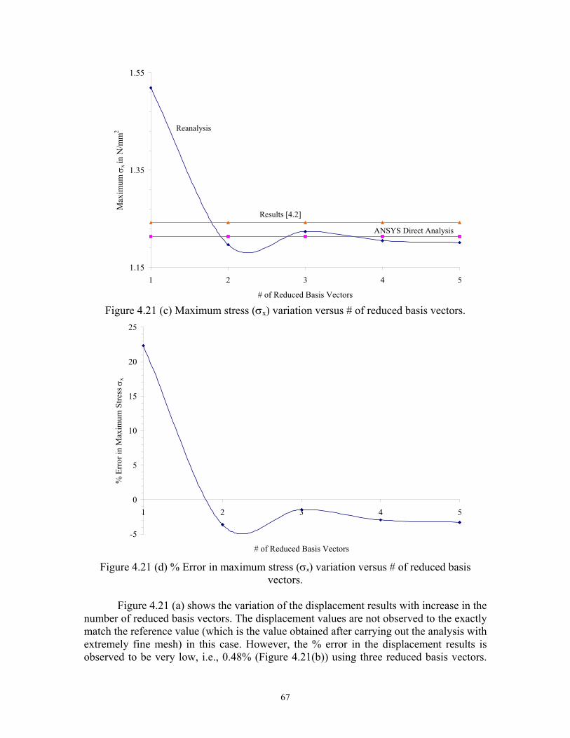
1.15

1.35

1.55

1 2 3 4

# of Reduced Basis Vectors

Max

imum

σx in

N/m

m2

Results [4.2]

ANSYS Direct Analysis

Reanalysis

5

Figure 4.21 (c) Maximum stress (σx) variation versus # of reduced basis vectors.

-5

0

5

10

15

20

25

1 2 3 4

# of Reduced Basis Vectors

% E

rror

in M

axim

um S

tress

σx

5

Figure 4.21 (d) % Error in maximum stress (σx) variation versus # of reduced basis

vectors. Figure 4.21 (a) shows the variation of the displacement results with increase in the

number of reduced basis vectors. The displacement values are not observed to the exactly match the reference value (which is the value obtained after carrying out the analysis with extremely fine mesh) in this case. However, the % error in the displacement results is observed to be very low, i.e., 0.48% (Figure 4.21(b)) using three reduced basis vectors.

67

Thus the results are acceptable. As far as the stress results are concerned, the % error in the stress when compared with the theoretical value (values given by Waldman [4.2] in his paper) is only 3.2 % with five reduced basis vectors. However, when the number of reduced basis vector equals to three the % error in the stress value is 1.44 %. This value of reduced basis vectors will be used in this work. As discussed by Gullickson [4.1], for fairly good accuracy and less computational efforts the number of reduced basis vectors should be kept as three.

4.3.3 Redesign Option # 2: Plate with Circular Arc Fillet

In this Redesign Option and the next, even though it is observed that the stress

concentration factor in Option # 1 is found to be lower, different geometric options for the fillet are explored to check the stress concentration factor. In this case the geometry is changed to a circular fillet at the corner as shown in Figure 4.18. Here a circular arc is added to reduce the stress concentration. A similar method of reanalysis is used and Figure 4.22 shows the contour plot of the stress and displacement results. The reanalysis will use the solution for the initial design discussed in Section 4.3.1 as the base for generating results for the new design option. The results are also presented in tabular form for displacement and stress in Tables 4.18 and 4.19, respectively.

Table 4.18 Maximum Deflections (mm)

UX UY Node # 27 1 Value 0.18024×10-3 -0.36539×10-4

Table 4.19 Minimum and Maximum stress components (N/mm2)

σx σy σxy σVM

Node # 52 10 48 60 Minimum Value -0.81206×10-2 0.18712 -0.4085 0.10157×10-1

Node # 50 49 1 50 Maximum Value 1.3890 0.30406 0.1×10-1 1.4096

68

Mesh Characteristics 125 Four-node Quad Elements 156 Nodes 2 DOF/Node 312 Total DOF Plane Stress

(a) Ux – Displacement (mm)

(b) σx – Normal Stress (N/mm2) (c) σVM – von Mises Stress (N/mm2)

Figure 4.22 Contour plot of results for Redesign Option # 2. In this problem, the number of reduced basis vectors is equal to three. The

analysis for varying the number of reduced basis vectors is not considered. Table 4.20 shows a comparison of these results with respect to the theoretical answer and also with respect to ANSYS solution when the same problem is solved using the ANSYS solver.

The results in Table 4.20 show that for displacements, % error is 0.68 % when

compared with the theoretical value. The theoretical value is based on the ANSYS solution for a very fine mesh (# of elements = 12500 and # of nodes = 12801). If the same is compared with the ANSYS direct analysis solution for the same mesh, then the % error is found to be 0.19%. For comparing stresses, (i.e., the stress concentration factor in this problem) when compared with the theoretical value, the % error is found to be 1.1%. The theoretical value is calculated in Appendix E. When compared with ANSYS direct analysis result for the same mesh yields 0.27 %.

69

Table 4.20 Comparison of results for Redesign Option # 2 Maximum Quantities Theoretical ANSYS Direct

Analysis Reanalysis +

Value 1.3734 1.3852 1.3890 σx N/mm2 Node # - 51 50

Value 1.3734 1.3932 1.4096 σVM N/mm2 Node # - 50 50

Value 0.18148∗ 0.18058 0.18024 Ux ×10-3 mm Node # - 27 27

Note: * Theoretical value of displacement is based on very fine mesh of four-node quadrilateral elements (# of elements = 12500, # of nodes = 12801). + Reanalysis based on initial design using three basis vectors.

4.3.4 Redesign Option # 3: Plate with Two Circular Arc Fillets

Redesign Option # 3 considers a small circular arc that is added at the two corners

of the fillet. The dimensions of the arcs can be found in Figure 4.18. The reanalysis results are shown in Figure 4.23 as contour plots and Tables 4.21 and 4.22 shows the displacement and stress results, respectively.

Mesh Characteristics 125 Four-node quadrilateral Elements 156 Nodes 2 DOF/Node 312 Total DOF Plane Stress

(a) Ux – Displacement (mm)

(b) σx – Normal Stress (N/mm2) (c) σvM – von Mises Stress (N/mm2)

Figure 4.23 Contour Plot of results for Redesign Option # 3.

70

Table 4.21 Maximum Deflections (mm) UX UY

Node # 12 1 Value 0.17517×10-3 -0.36403×10-4

Table 4.22 Minimum and Maximum stress components (N/mm2)

σx σy σxy σVM

Node # 52 11 50 60 Minimum Value -0.111×10-1 0.1759 -0.31285 0.13267×10-1

Node # 33 32 11 33 Maximum Value 1.2913 0.20431 0.10479 1.2749 The number of reduced basis vectors is equal to three in this redesign option. The

analysis for varying the number of reduced basis vectors from one to five is not considered. Table 4.23 shows the comparison of these results with respect to the theoretical answer and also with respect to ANSYS solution when the same problem is solved using the ANSYS solver. The theoretical value of stress concentration factor for this geometry is not available therefore, a very fine mesh was used.

Table 4.23 Comparison of maximum results for Redesign Option # 3. Maximum Quantities Theoretical ANSYS Reanalysis+

Value 1.3224∗ 1.288 1.2913 σx N/mm2 Node # - 33 33

Value 1.3408∗ 1.2727 1.2749 σvM N/mm2 Node # 33 33

Value 0.17591∗ 0.17543 0.17517 UX ×10-3 mm Node # - 12 12

Note: * Theoretical value of displacement is based on a very fine mesh of four-node quadrilateral elements (# of elements = 12500, # of nodes = 12801) + Reanalysis based on initial design using three basis vectors.

The results in Table 4.23 show that for displacements, % error is 0.42 % when

compared with the theoretical value and is 0.15 % when compared with the ANSYS direct analysis solution for the same mesh. When comparing stresses (i.e., the stress concentration factor in this problem) with the theoretical value, the % error is found to be 2.35% whereas, when compared with ANSYS direct analysis result for the same mesh it is found to be 0.26 %.

4.3.5 Conclusion for Case Study # 2

The main objective in this problem was to use the reanalysis method to verify

whether the same results are obtained for Kt using the free-form geometry of the fillet as discussed by Waldman [4.2]. The stress concentration factor values obtained by

71

reanalysis for the free-form geometry were observed to be consistent with the values obtained by Waldman resulting in an error of 1.44%. By keeping the number of reduced basis vectors to be equal to three, fairly accurate results were obtained for stresses. Therefore, in future case studies only three reduced basis vectors will be used. Table 4.24 provides a comparison of results for all fillet shapes.

Table 4.24 Comparison of maximum results for the three redesign options.

Redesign Options

# 1: Free-form Fillet # 2: Circular Arc Fillet # 3: Two Circular ArcsMaximum Quantities ANSYS

Direct Analysis

Reanalysis+ ANSYS Direct

Analysis Reanalysis+

ANSYS Direct

Analysis Reanalysis+

σx N/mm2 1.2138 1.2241 1.3852 1.3892 1.288 1.2913

σVM N/mm2 1.2127 1.2180 1.3932 1.4096 1.2727 1.2749

Ux (× 10-3 mm) 0.18562 0.18524 0.18058 0.18024 0.17543 0.17517

+ Reanalysis results are based on three reduced basis vectors. 4.4 Case Study # 3: Support Bracket Redesign Case Study # 3 considers the redesign of support. The idea is to design a support which will act as a cantilever beam, will support a load at the end and will be fixed on two pin holes. Figure 4.24 shows the geometry of the initial design and three redesign options considered. Figure 4.25 shows the dimensions for the initial design and the three redesign options. The finite element models have the same geometry. The pins are represented by nodes lying on the circle that are constrained in X and Y translational DOFs. A point load of 50 N is applied at the free end. The following items are considered by the engineer in the redesign process:

1. The support shown in Figure 4.24 is loaded such that the maximum stress will be at the fillet due to a compressive bending stress.

2. The stress varies linearly with the distance from the load application point. The area in the vicinity of the point force is under-stressed. Therefore, the cross-sectional thickness can be reduced in this region.

3. The maximum stress will reduced by increasing the fillet radius.

72

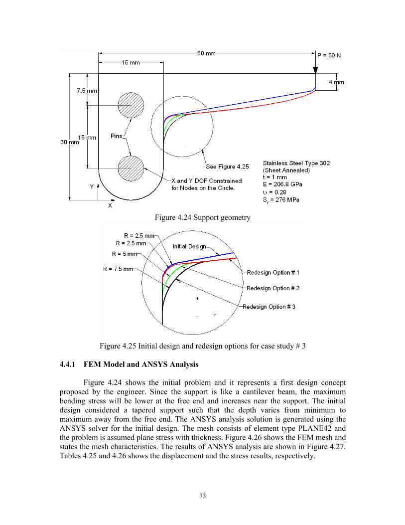
Figure 4.24 Support geometry

.4.1 FEM Model and ANSYS Analysis

Figure 4.24 shows the initial problem and it represents a first design concept propos

Figure 4.25 Initial design and redesign options for case study # 3

4

ed by the engineer. Since the support is like a cantilever beam, the maximum bending stress will be lower at the free end and increases near the support. The initial design considered a tapered support such that the depth varies from minimum to maximum away from the free end. The ANSYS analysis solution is generated using the ANSYS solver for the initial design. The mesh consists of element type PLANE42 and the problem is assumed plane stress with thickness. Figure 4.26 shows the FEM mesh and states the mesh characteristics. The results of ANSYS analysis are shown in Figure 4.27. Tables 4.25 and 4.26 shows the displacement and the stress results, respectively.

73

Figure 4.26 FEM Mesh for Initial Design of Case Study # 3.

ments Mesh Characteristics 349 Four-node Quad Ele415 Nodes 2 DOF/Node 830 Total DOF Plane Stress

Con l

(b) USUM– Displacement vector sum (mm) (a) Ux – Displacement (mm)

(c) σx – Normal Stress (N/mm2) (d) σVM – von Mises Stress at Fillet (N/mm2)

Figure 4.27 tour p ot of results.

74

Table 4.25 Maximum Deflections (mm) UX UY

Node # 43 43 Value 0.18767 × 10-1 -0.9685 × 10-1

Table 4.26 Minimum and Maximum stress components (N/mm2)

σx σy σxy σvM

Node # 2 43 5 176 Minimum Value -129.61 -121.55 -62.146 0.27448 Node # 56 192 179 5 Maximum Value 108.30 19.739 33.690 152.59

One can observe that the absolute maximum stress is at the fillet and is

compressive. The von Mises stress at the fillet is 152.6 N/mm2. The material has yield strength of 276 N/mm2 resulting in a safety factor of 1.81. The aim in this redesign process is to have an optimum shape with a safety factor of about 2.

4.4.2 Redesign Option # 1: Optimum thickness for uniform stress distribution

The tapered shape is designed to have a uniform stress distribution as discussed earlier. From Figure 4.27 (d) it can be seen that the von Mises stress distribution is approximately uniform at the outer fiber. A straight taper is not the optimum shape for a uniform stress distribution. For the cantilever beam with point load we know that the bending stress varies linearly. The maximum at the support end and minimum, i.e., zero at the end where the load is getting applied. Therefore, at any distance x from the load, the maximum bending stress is,

3max

121

2)(

hb

hxP

IyM

x⋅⋅

⋅⋅=

⋅=σ

where, maxxσ = Maximum bending stress allowable.

P = Applied load. h = Height of cross-sectional area b = Width of cross section (it is the thickness for the plane stress problem which is 1.) Using this information the variation of height h with respect to x is given as,

xPh ⋅⋅

=σ

6

This equation shows that for uniform bending stress distribution, the height h must be function of x . Thus, for Redesign Option # 1 the geometry is modified to be the function of x as shown in Figure 4.28(a). Tables 4.27 and 4.28 state the displacement and stress results for the reanalysis, respectively. The contour plots of the results are shown in Figure 4.28.

75

Table 4.27 Maximum Deflections (mm) UX UY

Node # 43 43 Value 0.15196 × 10-1 -0.74779 × 10-1

Table 4.28 Minimum and Maximum stress components at fillet (N/mm2)

σx σy σxy σVM

Node # 2 43 5 176 Minimum Value -142.37 -124.86 -62.044 0.25278 Node # 51 192 179 5 Maximum Value 96.196 19.546 33.477 159.40

(a) FE Mesh for the Model (b) USUM– Displacement Vector Sum (mm)

(c) σx – Normal Stress (N/mm2) (d) σVM – von Mises Stress (N/mm2)

Figure 4.28 Contour plots for Redesign Option # 1. The von Mises Stress contour plot shows that the stress is approximately uniform

throughout the length of the support. To compare the reanalysis results, the same mesh is solved using the ANSYS solver (ANSYS Direct Analysis) and a fine mesh (# of elements

76

= 1508, # of nodes = 1654) to obtain the displacement and the stress results at the fillet. Table 4.29 shows a comparison of all these results. The reanalysis is based on three reduced basis vectors.

Table 4.29 Comparison of maximum results for Redesign Option # 1. Maximum Quantities Fine Mesh* ANSYS Direct

Analysis Reanalysis +

Value -152.47 -138.77 -142.37 Compressive σx

N/mm2 Node # - 2 2

Value 165.71 152.39 159.40 σVM N/mm2 Node # - 5 5

Value −0.74888 -0.74787 -0.74779 UY ×10-1 mm Node # - 43 43

* Theoretical value of displacement is based on a very fine mesh of four-node quadrilateral elements (# of elements = 1508, # of nodes = 1654) + Reanalysis based on initial design using three basis vectors. The result demonstrates that for three reduced basis vectors yields a % error in

maximum displacement UY of 0.01% when compared to the ANSYS Direct Analysis. Being higher in absolute value, UY is considered as the basis of comparison. The % error in the maximum compressive stress σx is 2.6 % compared with ANSYS direct analysis results and is 6.6% when compared with the fine mesh. The von Mises stress yields the % error of 4.6 % compared with the ANSYS direct analysis and 3.8 % when compared with the fine mesh. Overall, the von Mises stresses the safety factor of 1.73. However, this value is too low since a factor of safety of 2 is required. Therefore, the fillet must be changed.

4.4.3 Redesign Option # 2: Fillet Radius of 5 mm

Keeping the optimum shape of the taper, the fillet radius is increased from 2.5 to

5 mm in Redesign Option # 2 as shown in Figure 4.25. The reason why the fillet size is increased is to reduce the stress level at the fillet in turn increasing the safety factor. After performing the reanalysis the results are presented in Tables 4.30 and 4.31 for displacement and stresses, respectively. Figure 4.29 shows the contour plots of results.

Table 4.30 Maximum Deflections (mm)

UX UY Node # 43 43 Value 0.14729 × 10-1 -0.70830× 10-1

77

Table 4.31 Minimum and Maximum stress components (N/mm2) σx σy σxy σVM

Node # 38 43 5 83 Minimum Value -122.11 -122.09 -45.530 0.24185 Node # 53 192 179 43 Maximum Value 94.405 16.467 30.070 140.95

Figure 4.29 Contour Plots for Redesign Option # 2

The maximum von Mises stress at the fillet has been reduced due to increase in

fillet size. Comparing the reanalysis results, the same mesh is solved using the ANSYS solver a very fine mesh (# of elements =1430, # of nodes = 1572). Table 4.32 shows a comparison of all these results. The reanalysis is based on three number of reduced basis vectors.

(b) USUM– displacement vector sum (mm)(a) FE Mesh for the Model

(c) σx – Normal Stress (N/mm2) (d) σVM – vonMises Stress (N/mm2)

78

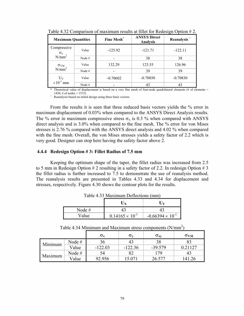
Table 4.32 Comparison of maximum results at fillet for Redesign Option # 2. Maximum Quantities Fine Mesh* ANSYS Direct

Analysis Reanalysis +

Value -125.92 -121.71 -122.11 Compressive

σx N/mm2 Node # - 38 38

Value 132.29 123.55 126.96 σVM N/mm2 Node # - 39 39

Value −0.70602 -0.70850 -0.70830 UY ×10-1 mm Node # - 43 43

* Theoretical value of displacement is based on a very fine mesh of four-node quadrilateral elements (# of elements = 1430, # of nodes = 1572) + Reanalysis based on initial design using three basis vectors.

From the results it is seen that three reduced basis vectors yields the % error in

maximum displacement of 0.03% when compared to the ANSYS Direct Analysis results. The % error in maximum compressive stress σx is 0.3 % when compared with ANSYS direct analysis and is 3.0% when compared to the fine mesh. The % error for von Mises stresses is 2.76 % compared with the ANSYS direct analysis and 4.02 % when compared with the fine mesh. Overall, the von Mises stresses yields a safety factor of 2.2 which is very good. Designer can stop here having the safety factor above 2.

4.4.4 Redesign Option # 3: Fillet Radius of 7.5 mm

Keeping the optimum shape of the taper, the fillet radius was increased from 2.5

to 5 mm in Redesign Option # 2 resulting in a safety factor of 2.2. In redesign Option # 3 the fillet radius is further increased to 7.5 to demonstrate the use of reanalysis method. The reanalysis results are presented in Tables 4.33 and 4.34 for displacement and stresses, respectively. Figure 4.30 shows the contour plots for the results.

Table 4.33 Maximum Deflections (mm)

UX UY Node # 43 43 Value 0.14165 × 10-1 -0.66394 × 10-1

Table 4.34 Minimum and Maximum stress components (N/mm2)

σx σy σxy σVM

Node # 36 43 38 83 Minimum Value -122.03 -122.36 -39.579 0.21127 Node # 54 82 179 43 Maximum Value 92.956 15.071 26.577 141.26

79

(a) FE Mesh (b) USUM– Displacement Vector Sum (mm)

(c) σx – Normal Stress (N/mm2) (d) σVM – von Mises Stress (N/mm2)

Figure 4.30 Contour plots for Redesign Option # 3 The reanalysis results, are compared to the ANSYS direct analysis solution and

also for a very fine mesh (# of elements = 1447, # of nodes = 1587). Table 4.35 shows a comparison of these results. The reanalysis is based on three reduced basis vectors.

80

Table 4.35 Comparison of maximum results for Redesign Option # 3. Maximum Quantities Fine Mesh* ANSYS Direct

Analysis Reanalysis +

Value -113.74 -118.58 -122.03 Compressive σx

N/mm2 Node # - 36 36 Value 117.98 118.40 121.79 σvM

N/mm2 Node # - 36 36 Value -0.60665 -0.66519 -0.66394 UY

×10-1 mm Node # - 43 43 * Theoretical value of displacement is based on a very fine mesh of four-node quadrilateral elements (# of elements = 1447, # of nodes = 1587) + Reanalysis based on initial design using three basis vectors. From the results it is seen that based on three reduced basis vectors the % error in

maximum displacement is 0.2 when compared to the ANSYS Direct Analysis results. The % error in maximum compressive stress σx is 2.9 % when compared with ANSYS direct analysis and it is 7.29% when compared with the fine mesh. The % error in is higher when compared with respect to the fine mesh but it is lower with respect to the ANSYS direct analysis which is really our base of comparison since it is the solution for the same mesh. The von Mises stresses the % error is 2.9 % compared with the ANSYS direct analysis results and 3.2 % when compared with fine mesh. Overall, the maximum von Mises stress yields a safety factor of 2.3 which is very high. Thus, it is good to use the redesign option # 2 which yields the safety factor of only 2.02 and it should be selected as the final design.

4.4.5 Conclusion for Case Study # 3

This problem demonstrates using reanalysis in design process to improve a

design. As shown, the initial design concept of the support is tried with three different design options and the finite element analysis of each was carried easily. In the initial design considered a tapered beam and the safety factor was 1.8. The shape was then modified to be optimum in Redesign Option # 1. It was found that besides yielding a uniform stress distribution, the fillet geometry reduced safety factor to 1.73. Thus, further modifications of the fillet radius were considered. In redesign Option # 2 the fillet radius was changed to 5 mm yielding a safety factor of 2.2. Furthermore, increasing the fillet radius to 7.5 yielded a larger safety factor of 2.3 providing the designer more design options. Table 4.36 provides a comparison of the results for initial and three redesign options. It can be observed that each design option reduced the von Mises stress at the fillet and also the displacement. This is also a criterion to be considered while reducing the cross section area.

81

Table 4.36 Comparison of results for the three redesign options. Design Options

Initial Design: Fillet Radius

2.5 mm

# 1: Optimum Shape of Taper

# 2: Fillet Radius 5 mm

# 3: Fillet Radius 7.5 mm

Maximum Quantities

ANSYS Direct Analysis

ANSYS Direct

Analysis Reanalysis+

ANSYS Direct

Analysis Reanalysis+

ANSYS Direct

Analysis Reanalysis+

Compressive σx

N/mm2 -129.61 -138.77 -142.37 -121.71 -122.11 -118.58 -122.03

σVM N/mm2 152.59 152.39 159.40 123.55 126.96 118.40 121.79

Safety Factor 1.8 1.8 1.7 2.2 2.2 2.3 2.3

UY (× 10-1 mm) -0.9685 -0.7479 -0.74779 -0.7085 0.7083 0.6652 0.66394

+ Based on three reduced basis vectors.

82

5. Conclusion A prototype graphically driven finite element reanalysis technique has been

developed for machine elements that can be used by an engineer/company in the initial design stage. A prototype has been integrated into the commercial finite element code ANSYS. The finite element system allows an engineer to modify part geometry and instantaneously view the results due to geometric changes. This means that the optimization process is engineer-driven as opposed to mathematically-driven. The anticipated advantages of using the technique in the initial design stage could result in a shortened time to market, improved product design and reduced product development cost for a company.

Three case studies were presented to demonstrate the usability, accuracy and

reliability of the prototype software system. The first case study considered a plate with a hole subjected to a tensile distributed load. Different hole geometries were explored to determine their effect on the stress concentration factor in a plate. An engineer can modify the geometry of a given hole and displacement and stress results can be instantaneously viewed. A reanalysis method is used to solve each modified problem and the same problem was solved using the ANSYS Direct solver to verify reanalysis accuracy. This was also done for the other two case studies. The numbers of reduced basis vectors used in the reanalysis were varied from one to five to explore displacement and stress solution accuracy. It was determined from the three case studies that as the number of reduced basis vectors increases, solution accuracy increased. Therefore, three reduced basis vectors should be used to reduce computational effort while maintaining accuracy.

The second case study considered a plate with a fillet under tension loading. The

goal was to obtain a fillet geometry that would minimize the stress concentration factor. In this case study the engineer, instead of trying traditional circular or elliptical fillets, can obtain better results by creating an optimum free-form fillet reducing the stress concentration.

The third case study considered a more practical problem then the first two which

are commonly found in undergraduate mechanics of materials textbooks. The problem considered redesigning a cantilever L-shaped support bracket subjected to a concentrated force at its free end. The optimum shape of the cantilever support was first determined by the engineer with the goal of obtaining a uniform stress distribution. After the optimum cantilever shape was obtained then different fillet sizes were explored at the intersection of the L-shaped bracket to obtain an optimum shape for a high safety factor.

83

6. Future Work

In the case studies in Chapter 4 it was shown how the combined approximation reanalysis method described in Section 2.4 can be used to solve a reanalysis finite element problem. The advantages of implementing the reanalysis method during the early design process are as follows:

1. Helps designer to consider and evaluate alternate approaches and explore design

options. 2. Reduces product development cost. 3. Helps in formulating an improved design. 4. Shortens the time to market. 5. Reduces the knowledge gap.

In spite of these advantages, the following five items are proposed as future work:

1. Improved ANSYS Output Environment. The system developed in this work is based on ANSYS 5.7. The new version of ANSYS is 6.1. Some portions of this work, such as accessing the ANSYS result file (file.rst), is not supported in version 6.1. Initially the idea was to use ANSYS 6.1, however, ANSYS technical support notified me that there are few bugs when reading the result file. They have modified the entire structure of result file. The newer and corrected method of reading and writing the result file will be implemented by ANSYS in their newest version that is currently being released. That is why this work used the older version, i.e., ANSYS 5.7. The FORTRAN code to read the result file need to be modified slightly depending on the structure of the result file for the newer release coupled with the advantage of the improved user friendly interface of ANSYS 6.1. Furthermore, since the GUI of ANSYS 6.1 has changed, especially the “Main Menu,” the current method developed in UIDL to modify the main menu must be modified to be compatible with ANSYS 6.1.

2. Use of Combined Approximation Method for Changing the Number of

DOFs. There are three types of changes which can be made to the finite element mesh as follows:

(a) When the nodes or elements are deleted, i.e., when the total number of DOFs is reduced.

(b) When the nodes and elements are added in the mesh, i.e., when the total number of DOF is increased. This is more analogous to mesh refinement.

(c) When the geometric positions of the nodes are changed keeping the total number of DOFs unchanged (considered in this work).

The combined approximation reanalysis method used in this work applies when there is a change in nodal coordinates, i.e., case (c) above. Thus, the method is applicable only when the total number of DOFs in the mesh remains the same and only when the nodal coordinates are changed. Reanalysis methods have also been developed when the total number of DOFs in the mesh is changed [5.1, 5.2],

84

i.e., case (b) above. Although such a method is available, no effort has been made in any literature to solve the finite element problem for stress applications. Kirsch [5.1] has used this method for structural reanalysis where he considered the optimization of structures. For layout optimization, this method is typically helpful when the members and joints are added or deleted during the solution process. Gullickson [5.2] has used this method in solving a one-dimensional finite element problem. However, he used this method for generating the displacement results and not stresses. The reanalysis method is very useful especially when there is a need to refine the mesh. Usage of combined approximation method to solve the mesh refinement problem will now be discussed. In order to utilize the CA method, a problem must be stated as follows. Consider the initial stiffness matrix K0, let F0 be the initial force vector and let u0 be the displacement solution for the system obtained after solving the force-displacement relationship,

(5.1) 000 uKF = Changes in the initial stiffness matrix are represented by K∆ , so the new stiffness matrix can be written as,

(5.2) KKK ∆+= 0 and the new analysis equation can be written as,

00 )( FuKKKu =∆+= (5.3) where u is the resulting new displacement solution vector. Consider refinement of the initial mesh and this means that K may be of a different size than K0. Thus, after the solution of the initial problem for u0, K0 must be expanded in order to allow the addition of K∆ . This is accompanied as follows,

=⇒

IK

KK0

0000 (5.4)

where I is the identity matrix. Also note that,

=

−−

IKK

001

010 (5.5)

in order to avoid re-solving the original analysis equation after each mesh refinement and/or change in the K matrix, the CA method will be used (similar to

85

Section 2.4.1) to approximate the solution to the new problem. As discussed the CA method, as discussed, uses a linear combination of s linearly independent basis vectors to approximate the displacement vector u associated with the new design or mesh. For a reduced basis approximation, the displacement are approximated by,

Bss uyuyuyuyu ⋅=⋅++⋅+⋅= K2211 (5.6) where uB is an array containing s vectors u as defined below, and ysuu K21, i are coefficients to be determined.

01 uu = 02 Buu −=(5.7)

02

1 uBu = … 01)( uBu s

s−−=

where u is the initial displacement vector and B is defined as, 0

(5.8) KKB ∆= −1

0 Substituting the expression for u in Equation (5.6) into Equation (5.3) and then pre-multiplying by u results in the equation of following form, T

B

(5.9) 0)( FuyKuu T

BBTB =

using, and . )( B

TBR KuuK = 0FuF T

BR = So similar to the expression derived in Section 2.4.2, Equation (5.9) reduces to,

RR FyK = (5.10) vector y can be determined by solving Equation (5.10). Thus remaining portion of this process is similar to the CA method explained in Section 2.4.2. Therefore, the CA method can be used for the case when not only the nodal coordinates are changed, but also when the total number of DOFs is changed.

3. Three-dimensional Problems. In this work, the reanalysis method was applied to only two-dimensional element types. The element type used here is ANSYS PLANE42. The method can be extended to three-dimensional element types, i.e., SOLID45, which has 8 nodes per element and 3 DOF per node and also plate and shell elements.

4. Contour Plot of Factor of Safety. ANSYS Parametric Design Language (APDL)

can be used to obtain a contour plot of the factor of safety for the component

86

being analyzed. The plot of the contour shape is similar to the stress contour plot. The designer will have to enter the yield stress for the material and ANSYS will generate a safety factor contour plot.

5. Fatigue Analysis. The method can also be extended to perform fatigue analysis

of the design problem. The designer will be able to obtain a contour plot regarding the safety of the design in fatigue.

6. Boundary Element Analysis. The combined approximation reanalysis method

can also be applied to boundary elements. In boundary elements only the boundary of the geometry is discretized. In stress analysis the maximum stresses almost all the time occurs on the boundary. Furthermore, in case of two-dimensional problems the boundary elements are only lines rather than areas in finite elements [5.3-5.4]. therefore, only nodes on the boundary are moved whereas nodes on the boundary and inside the boundary need to be changed. The reanalysis method can be combined with boundary elements should result in an analysis that is faster and more accurate.

Figure 6.1 shows the similar form of boundary element mesh for the FE mesh shown in Figure 3.4. Same nodes are moved to show the similarity between two problems.

1 2 3 4

5 8

9

13 14 15 16

NodeNumbers

12

14 15

1 4

5 8

9

13 16

2 3

12

b) Modified Mesha) Initial Mesh

Node Coordinates Changed

Figure 6.1 BE Mesh

87

References

[1.1] Norton, R.L., MACHINE DESIGN An Integrated Approach, Second Edition, Prentice-Hall, Upper Saddle River, NJ (2000).

[1.2] Ertas, A. and Jones, J.C., The Engineering Design Process, John Wiley & Sons,

Inc., New York, NY (1993). [1.3] Dimarogonas, A.D., Machine Design A CAD Approach, John Wiley & Sons, Inc.,

New York, NY (2000).

[1.4] Suh, N.P., AXIOMATIC DESIGN Advances and Applications, Oxford University Press, New York, NY (2001).

[1.5] Juvinall, R.C. and Marshek, K.M., Fundamentals of Machine Component Design, Third Edition, Jon Wiley & Sons, Inc., New York, NY (1999).

[1.6] Zahavi, E., The Finite Element Method in Machine Design, A Solomon Press Book, Prentice Hall, Englewood Cliffs, NJ (1992).

[1.7] “Enterprise-wide Solutions: Product Design, Analysis and Management through Engineering Teamwork,” ANSYS White Paper, ANSYS Inc. Houston, PA (2002),

http://www.ansys.com/customer_stories/white_papers.htm

[1.8] Berry, D.T. and Leewood, A.R., “FEA for Production Design,” Machine Design, pp. 66-67, (September 21, 1989).

[1.9] Szabo, B.A. and Actis, R.L., “Finite Element Analysis in Professional Practice”, Computer Methods in Applied Mechanics and Engineering, v.133 pp. 209-228 (1996).

[1.10] Roth, G., “The Value of Early Analysis (Part 1),” NAFEMS Publications, East

Kilbride, G750 QD, UK (July 2000), http://www.nafems.org/publications/downloads/Article2.pdf.

[1.11] Cotnoir, P., MFE 540 Design For Manufacturability, Worcester Polytechnic

Institute, Worcester MA, Class Notes for Spring (2002). [1.12] Hamrock, B.J., Jacobson, B. and Schmid S.R., Fundamentals of Machine

Elements, WCB McGraw-Hill, Boston, MA (1999). [1.13] Shigley, J. E. and Mischke, C. R., Mechanical Engineering Design, McGraw Hill

Boston, MA (2001). [1.14] Adams, V. and Askenazi, A., Building Better Products with Finite Element

Analysis, Onward Press, Santa Fe, NM (1999).

88

[1.15] Kirsch, U., Optimum Structural Design-Concepts, Methods and Applications, McGraw-Hill, New York, NY (1981).

[1.16] Kirsch U. and Papalambros P.Y., “Exact and Accurate Reanalysis of Structures

for geometrical Changes,” Engineering with Computers, v. 17, pp. 363-372 (2001).

[2.1] Kirsch, U., Optimum Structural Design-Concepts, Methods and Applications,

McGraw-Hill, New York, NY, (1981).

[2.2] Whitesell, J.E., “Rational Approximation in Structural Design Reanalysis,”

Journal of Mechanism Transmissions and Automation in Design, v. 106, pp. 114-118, (March 1984).

[2.3] Kirsch, U. and Toledano G., “Approximate Reanalysis for Modifications of

Structural Geometry,” Computers and Structures, v. 16, n. 1-4, pp. 269-277, (1983).

[2.4] Huang, C. and Verchery, G., “An Exact Structural Reanalysis,” Communications

in Numerical Methods in Engineering, v. 103, pp. 103-112, (1997). [2.5] Householder, A.S., “A Survey of Some Closed Methods for Inverting Matrices,”

SIAM Journal, v. 5, n. 3, pp. 155-169, (September 1957). [2.6] Abu Kassim A.M. and Topping B.H.V., “Static Reanalysis: A Review,” ASCE

Journal of Structural Division, v. 113, n. 5, pp. 1029-1045, (1987). [2.7] Sobieszezanski-Sobieski, J. and Haftka, R.T., “Multidisciplinary Aerospace

Design Optimization: Survey and Recent Development,” Structural Optimization, v. 14, pp. 1-23, (1997).

[2.8] Fox, R.L. and Miura, H., “An Approximate Analysis Technique for Design

Calculations,” AIAA Journal, v. 9, pp. 177-179, (1971). [2.9] Noor, A.K., “Recent Advances and Applications of Reduced Methods,” Applied

Mechanical Reviews, v. 47, pp. 125-146, (1994). [2.10] Feury, C., “Efficient Approximation Concepts Using Second Order Information,”

International Journal of Numerical Methods in Engineering, v. 28, pp. 2041-2058 (1989).

[2.11] Kirsch, U. and Liu, S., “Exact Structural Reanalysis by First Order Reduced Basis

Approach,” Structural Optimization, v. 10, pp. 153-158, (1995). [2.12] Kirsch, U. and Liu, S., “Structural Reanalysis for General Layout Modifications,”

AIAA Journal, v. 35, n. 2, pp. 382-388, (February 1997).

89

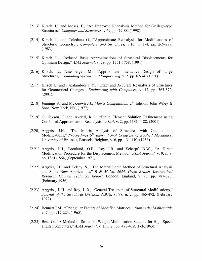
[2.13] Kirsch, U. and Moses, F., “An Improved Reanalysis Method for Grillage-type Structures,” Computer and Structures, v.69, pp. 79-88, (1998).

[2.14] Kirsch U. and Toledano G., “Approximate Reanalysis for Modifications of

Structural Geometry”, Computers and Structures, v.16, n. 1-4, pp. 269-277, (1983).

[2.15] Kirsch U., “Reduced Basis Approximations of Structural Displacements for

Optimum Design,” AIAA Journal, v. 29, pp. 1751-1758, (1991). [2.16] Kirsch, U., Aisenberger, M., “Approximate Interactive Design of Large

Structures,” Computing Systems and Engineering, v. 2, pp. 67-74, (1991). [2.17] Kirsch U. and Papalambros P.Y., “Exact and Accurate Reanalysis of Structures

for Geometrical Changes,” Engineering with Computers, v. 17, pp. 363-372, (2001).

[2.18] Jennings A. and McKeown J.J., Matrix Computation, 2nd Edition, John Wiley &

Sons, New York, NY, (1977). [2.19] Gullickson, J. and Averill, R.C., “Finite Element Solution Refinement using

Combined Approximation Reanalysis,” AIAA, v. 2, pp. 1181-1188, (2001). [2.20] Argyris, J.H., “The Matrix Analysis of Structures with Cutouts and

Modifications,” Proceedings 9th International Congress of Applied Mechanics, University of Brussels, Brussels, Belgium, v. 6, pp. 131-140, (1956).

[2.21] Argyris, J.H., Bronlund, O.E., Roy J.R. and Scharpf, D.W., “A Direct

Modification Procedure for the Displacement Method,” AIAA Journal, v. 9, n. 9, pp. 1861-1864, (September 1971).

[2.22] Argyris, J.H. and Kelsey, S., “The Matrix Force Method of Structural Analysis

and Some New Applications,” R & M No. 3034, Great British Aeronautical Research Council Technical Report, London, England, v. 93, pp. 787-828, (February 1956).

[2.23] Argyris , J. H. and Roy, J. R., “General Treatment of Structural Modifications,”

Journal of the Structural Division, ASCE, v. 98, n. 2, pp. 465-492, (February 1972).

[2.24] Bennett J.M., “Triangular Factors of Modified Matrices,” Numerishe Mathematik,

v. 7, pp. 217-221, (1965). [2.25] Best, G., “A Method of Structural Weight Minimization Suitable for High-Speed

Digital Computers,” AIAA Journal, v. 1, n. 2., pp. 478-479, (Feb.1963).

90

[2.26] Best, G.C., “The Stress-Area Method of Designing Beams,” Journal of Aeronautical Science, v.12, n. 3, pp. 298-304, (July 1945).

[2.27] Bhatia, K.G., “Rapid Iterative Reanalysis for Automated Design,” NASA TN D-

7357, NASA, Washington, D.C., (1973). [2.28] Celik, T., “Nonlinear Moment curvature Analysis by Means of Theorems of

Structural Variation,” Istanbul Devlet Muhendislik ve Mimarlik Akademisi Dergisi, v. 6, pp. 81-103, (1981).

[2.29] Celik, T., “The Theorems of Structural Variation and Their Application in the

Elastic-plastic Analysis of Frames,” Istanbul Devlet Muhendislik ve Mimarik Akademisi Dergisi, v. 5, pp. 125-138, (1979).

[2.30] Das, P.C., “Reanalyzing Structures with Small Modifications,” Computer Aided

Design, v. 10, n. 6, pp. 371-374, (November 1978). [2.31] Ding. H. and Gallagher, R.H., “Approximate Force Method Reanalysis

Techniques in Structural Optimization,” International Journal for Numerical Methods in Engineering, v. 21, pp. 1253-1267, (1985).

[2.32] Ertas, R. and Fenves, S.J., “Automatic Analyzer for Iterative Design,” Civil

Engineering Studies, Structural Research Series No. 352, University of Illinois, Urban, IL, (1969).

[2.33] Fetcher, R. and Powell, M.J.D., “On the Modification of LDLT Factorization,”

Mathematics of Computation, v. 28, n. 128, pp. 1067-1087, (October 1974). [2.34] Fox. R.L. and Miura, H., “An Approximate Analysis Technique for Design

Calculations,” AIAA Journal, v. 9, n. 1, pp. 177-179, (January 1971). [2.35] Gill, P.E., Golub, G.H. Murray, W. and Saunders, M. A., “Methods for Modifying

Matrix Factorizations,” Mathematics of Computation, v. 28, n.126, pp. 505-535, (April 1974).

[2.36] Gill, P.E., Murray, W. and Saunders, M. A., “Methods for Computing and

Modifying the LDV Factors of a Matrix,” Mathematics of Computation, v. 29, n. 132, pp. 1051-1077, (October 1975,).

[2.37] Goodey, W.J., “Solution of Modified Linear Simultaneous Equations,” Air-craft

Engineering, v. 31, pp. 358-359 and 364, (December 1959). [2.38] Hoerner, S.V., “Homologous Deformations of Tiltable Telescopes,” Journal of

the Structural Division, ASCE, v. 93, n. 5, pp. 461-485, (October 1967).

91

[2.39] Householder, A.S., Principles of Numerical Analysis, McGraw-Hill Book Company, New York, NY, (1953).

[2.40] Householder, A.S., “A Survey of Some Closed Methods for Inverting Matrices,”

SIAM Journal, v. 5, n. 3, pp. 155-169 (September, 1957). [2.41] Householder, A.S., The Theory of Matrices in Numerical Analysis, Blaisdell

Publishing Company, New York, NY, (1964). [2.42] Kavanagh, K.T., “An Approximate Algorithm for the Reanalysis of Structures by

the Finite Element Method,” Computers and Structures, v. 2, pp. 713-722, (1972). [2.43] Kirsch, U., “Approximate Structural Reanalysis Based on Series Expansion,”

Computer Methods in Applied Mechanics and Engineering, v. 26, pp. 205-223, (1981).

[2.44] Kirsch, U., “Approximate Structural Reanalysis for Optimization Along a

Lines,” International Journal for Numerical Methods in Engineering, v. 18, pp. 635-651, (1982).

[2.45] Kirsch, U. and Hoffman, B., “Approximate Behavior Models for Optimum

Structural Designs,” Proceedings International Symposium on Optimum Structural Design, Tuscan, AZ, pp. 7.17-7.26, (1981).

[2.46] Kirsch, U. and Rubinstein, M.F., “Modification of Structural Analysis by the

Solution of a Reduced Set of Equations,” UCLA Paper ENG-0570, University of California, Los Angeles, CA, (1970).

[2.47] Kirsch, U. and Rubinstein, M.F., “Reanalysis for Limited Structural Design

Modifications,” Journal of the Engineering Mechanics Division, ASCE, v. 98, n. 1, pp. 61-70, (February 1972).

[2.48] Kirsch, U. and Rubinstein, M.F., “Structural Reanalysis by Iteration,” Computers

and Structures, v. 2, pp. 497-510, (1972). [2.49] Kirsch, U. and Toledano, G., “Approximate Reanalysis for Modifications of

Structural Geometry,” Computers and Structures, v. 16, pp. 269-277, (1983). [2.50] Kleiber, M. and Lutoborski, A., “Modified Triangular Factors in the Incremental

Finite Element Analysis with Non-symmetric Stiffness Change,” Computers and Structures, v. 9, pp. 599-602, (1978).

[2.51] Kosko, E., “Effect of Local Modifications in Redundant Structures,” Journal of

the Aerospace Science, v. 21, n. 3, pp. 206-207, (March 1954).

92

[2.52] Kosko, E., “Matrix Inversion by Partitioning,” Aeronautical Quarterly, v. 8, pp. 157-184, (May 1957).

[2.53] Law, K.H., “Sparse Matrix Factor Modification in Structural Reanalysis,”

International Journal for Numerical Methods in Engineering, v. 21, pp. 37-63, (1985).

[2.54] Law, K.H. and Fenves, S.J., “Sparse Matrices, Graph Theory, and Reanalysis,”

Proceedings of the International Conference in Civil Engineering, ASCE, New York, NY, pp. 234-249, (May 12-14 1981).

[2.55] McNeal, R.H., “Application of the Compensation Theorem to the Modification of

Redundant Structures,” Journal of the Aeronautic Scientist, v. 20, n. 10, pp. 726-727, (October 1953).

[2.56] Majid, K.I., and Elliott, D.W.C., “Forces and Deflections in Changing

Structures,” The Structural Engineer, v. 51, n. 3, pp. 93-101, (March 1973). [2.57] Majid, K.I. and Elliott, D.W.C., “Topological Design of Pin Jointed Structures by

Non-linear Programming,” Proceedings of the Institution of Civil Engineers, v. 55, n. 2, pp. 129-149, (March 1973).

[2.58] Majid, K.I. and Saka, M.P., “Optimum Shape Design of Rigidly Jointed Frames,”

Proceedings of the Symposium on the Application of Computer Methods in Engineering, v. 1, University of Southern California, Los Angeles, CA, pp. 521-531.

[2.59] Majid, K.I., Saka, M.P. and Celik, T., “The Theorems of Structural Variation

Generalized for Rigidity Jointed Frames,” Proceedings of the Institution of Civil Engineering, v. 65, n. 2, pp. 839-856, (December 1978).

[2.60] Melosh, R.J., “Structural Analysis, Frailty Evaluation and Redesign,” Tech Report

No. TR-70-15, v. 1, Air Force Flight Dynamics Lab., Wright-Patterson Air Force Base, Dayton, OH (1970).

[2.61] Melosh, R.J., Johnson, J.R. and Luik, R., “Survivability Analysis of Structure,”

Proceedings of the 2nd, Conference on Matrix Methods in Structural Mechanics, AFFDL-TR-68-150, Wright-Patterson Air Force Base, Dayton, OH (December 1969).

[2.62] Melosh, R.J. and Luik, R., “Approximate Multiple Configuration Analysis and

Allocation for Least Weight Structural Design,” AFFDL-TR-67-59, Wright-Patterson Air Force Base, Dayton, OH (1967).

93

[2.63] Melosh, R.J. and Luik, R., “Multiple Configuration Analysis of Structures,” Journal of the Structural Division, ASCE, v. 94, n. 11, pp. 2581-2596, (November 1968).

[2.64] Melosh, R.J. and Luik, R., “Closure on Multiple Configuration Analysis of

Structures,” Journal of the Structural Division, ASCE, v. 96, n. 6, pp. 1239-1241, (June 1970).

[2.65] Mohraz, B. and Wright, R.N., “Solving Topologically Modified Structures,”

Computers and Structures, v. 3, pp. 341-353, (1973). [2.66] Noor, A.K., “Multiple Configuration Analysis via Mixed Method,” Journal of the

Structural Division, ASCE, v. 100, n. 9, pp. 1991-1997, (September 1974). [2.67] Noor, A.K. and Lowder, H.E., “Approximate Reanalysis Techniques with Sub

structuring,” Journal of the Structural Division, ASCE, v. 101, n. 8, pp. 1687-1698, (August 1975).

[2.68] Noor, A.K. and Lowder, H.E., “Approximate Techniques of Structural

Reanalysis,” Computers and Structures, v. 4, pp. 801-812, (1974). [2.69] Noor, A.K. and Lowder, H.E., “Structural Reanalysis via a Mixed Method,”

Computers and Structures, v. 5, pp. 9-12, (1975). [2.70] Phansalkar, S.R., “Matrix Iterative Methods for Structural Reanalysis,”

Computers and Structures, v. 4, pp. 779-800, (1974). [2.71] Row, D.G., Powell, G.H. and Mondkar, D.P., “Solution of Progressively

Changing Equilibrium Equations for Nonlinear Structures,” Computers and Structure, v. 7, pp. 659-665, (1977).

[2.72] Sack, R.L., Carpenter, W.C. and Hatch, G.L., “Modification of Elements in the

Displacement Method,” AIAA Journal, v.5, n. 9, pp. 1708-1710, (September 1967).

[2.73] Sobieszczanski, J., “Evaluation of Algorithms for Structural Modification,”

Proceedings of the Conference on Finite Element Methods in Civil Engineering, Vanderbilt University, Nashville, TN, pp. 129-153, (1969).

[2.74] Sobieszczanski, J., “Structural Modification by Perturbation Method,” Journal of

the Structural Division ASCE, v. 94, n. 12, pp. 2799-2816, (December 1968). [2.75] Storaasli, O.O. and Sobieszczanski, J., “Design Oriented Structural Analysis,”

AIAA Paper, pp. 73-538, Williamsburg, VA, (1973).

94

[2.76] Storaasli, O.O. and Sobieszczanski, J., “On the Accuracy of Taylor Approximation,” AIAA Journal, v. 12, n. 2, pp. 231-233, (February 1974).

[2.77] Topping, B.H.V., “The Application of the Theorems of Structural Variation to

Finite Element Problems,” International Journal for Numerical Methods in Engineering, v. 19, pp. 141-144, (1983).

[2.78] Topping, B.H.V. and Chan, H.F., “An Exact Formulation of the Theorems of

Geometric Variation for Statically Indeterminate Trusses,” Report, Department of Civil Engineering, University of Edinburgh, Edinburgh, UK, (1983).

[2.79] Wang, B.P. and Pilkey, W.D., “Efficient Reanalysis of Locally Modified

Structures,” Proceedings 1st, Chautagua on Finite Element Modeling, Schaeffer Analysis, pp. 37-61, (1980).

[2.80] Wang, B.P. and Pilkey, W.D., “Efficient Reanalysis of Locally Modified

Structures,” Department of Mechanical and Aerospace Engineering, Virginia University, Charlottesville, VA, (1980).

[2.81] Wang, B.P. and Pilkey, W.D., “Parameterization in Finite Element Analysis,”

Proceedings International Symposium on Optimum Structural Design, Tuscan, AZ, pp. 7.1-7.7, (1981).

[2.82] Wang, B.P., Pilkey, W.D. and Palazzaolo, A.R., Discussion on “Reanalysis

Modal Synthesis and Dynamic Design,” State-of-Art Surveys on Finite Element Technology, A. K. Noor, and W. D. Pickey, Eds., American Society of Mechanical Engineers, New York, NY, pp. 225-295 (1983).

[2.83] Weiner, B.L., “Variation of Coefficients of Simultaneous Linear Equations,”

Transaction of ASCE, v. 113, pp. 1349-1390, (1948). [2.84] Yang, W.H., “A Method for Updating Cholesky Factorization of a Band Matrix,”

Computer Methods in Applied Mechanics and Engineering, v. 12, pp. 281-288, (1977).

[2.85] Zielke, G., “Inversion of Modified Symmetric Matrices,” Journal of the

Association for Computing Machinery, v. 15, n. 3, pp. 402-408, (July 1968). [2.86] Kavlie, D. and Powell, G.H., “Efficient Reanalysis of Modified Structures,”

Journal of Structural Division, ASCE, v. 97, n. 1, pp. 377-392, (January 1971). [2.87] Wiberg, N.E., Discussion of “Efficient Reanalysis of Modified Structures,” by

Kavlie, D., and Powell, G. H., Journal of Structural Division ASCE, v. 97, n. 10, pp. 2612-2619, (October 1971)

95

[3.1] “Guide to ANSYS User Programmable Features,” ANSYS Release 5.6, ANSYS Inc., Canonsburg, PA (February 2000).

[3.2] Moaveni S., FINITE ELEMENT ANALYSIS Theory and Application with ANSYS,

Prentice Hall, Upper Saddle River, NJ (1999). [3.3] “Introduction to ANSYS 5.7 Part 1,” Training Manual, ANSYS Inc., Canonsburg,

PA (January 2001). [3.4] “APDL Programmer’s Guide,” ANSYS Release 5.6, ANSYS Inc., Canonsburg, PA

(February 2000). [3.5] “Guide to Interfacing with ANSYS,” ANSYS Release 5.6, ANSYS Inc.,

Canonsburg, PA (February 2000). [3.6] “Basic Analysis Procedures Guide,” ANSYS Release 5.6, ANSYS Inc.,

Canonsburg, PA (2003) http://www1.ansys.com/customer/content/documentation /60/Hlp_G_BAS1.html

[3.7] “ANSYS Command Reference,” ANSYS Release 5.6, ANSYS Inc., Canonsburg,

PA (2003) http://www1.ansys.com/customer/content/documentation/60/ Hlp_C_CmdTOC.html

[4.1] Gullickson, J. and Averill, R.C., “Finite Element Solution Refinement using

Combined Approximation Reanalysis,” American Institute of Aeronautics and Astronautics, v. 2, pp. 1181-1188, (2001).

[4.2] Waldman W., Heller M. and Chen G. X., “Optimal Free-form Shapes for

Shoulder Fillets in Flat Plates under Tension and Bending,” International Journal of Fatigue, v. 23, pp. 509-523, (2001).

[4.3] Pilkey, W.D., Peterson’s Stress Concentration Factors, Second Edition, John

Wiley & Sons Inc., New York, NY (1997). [4.4] Thompson, D.W., On Growth and Form Vol. 2, Second Edition, Cambridge

University Press, New York, NY (1963).

[5.1] Kirsch, U. and Liu, S., “Structural Reanalysis for General Layout Modifications,” American Institute of Aeronautics and Astronautics Journal, v. 35, n. 2, pp. 382-388, (February 1997).

[5.2] Gullickson, J. and Averill, R.C., “Finite Element Solution Refinement using

Combined Approximation Reanalysis,” American Institute of Aeronautics and Astronautics Journal, v. 2, pp. 1181-1188, (2001).

96

[5.3] Brebia, C. A. and Dominguez J., Boundary Elements An Introductory Course, McGraw-Hill Book Company, New York, NY (1989)

[5.4] Banerjee, P. K., The Boundary Element Method in Engineering, McGraw-Hill

Book Company, New York, NY (1993) [A.1] “Guide to Interfacing with ANSYS,” ANSYS Release 5.6, ANSYS Inc.,

Canonsburg, PA (February 2000). [B.1] “APDL Programmer’s Guide,” ANSYS Release 5.6, ANSYS Inc., Canonsburg, PA

(February 2000). [B.2] “ANSYS Command Reference,” ANSYS Release 5.6, ANSYS Inc., Canonsburg,

PA, http://www1.ansys.com/customer/content/documentation/60/ Hlp_C_CmdTOC.html

[C.1] Ciarlet, P.G., Introduction to Numerical Linear Algebra and Optimization, English Edition, Cambridge University Press, New York, NY (1988). [C.2] Jennings A. and McKeown, J.J., Matrix Computation, Second Edition, John

Wiley and Sons, New York, NY (1992). [C.3] Golub, G.H. and Van Loan, C.F., Matrix Computations, Second Edition, The John

Hopkins University Press, Baltimore, MD (1989). [E.1] Norton, R.L., MACHINE DESIGN An Integrated Approach, Second Edition, Prentice-Hall, Upper Saddle River, NJ (2000). [E.2] Pilkey, W.D., Peterson’s Stress Concentration Factors, Second Edition, John

Wiley & Sons Inc., New York, NY (1997).

97

A. ANSYS Result File (file.rst) Overview A.1 Overview A brief description of the result file generated by ANSYS [A.1] is presented in this appendix. ANSYS writes several binary files to store data created by an analysis. These files are named Jobname.Ext, where Jobname is the name of analysis file that caused the file to be generated and .Ext is an extension indicating the type of data in the file. Characteristics of ANSYS binary files are as follows:

1. An ANSYS binary file is a direct access, unformatted file. The record can be read or written by specifying (as a number) what location to read or write.

2. Before ANSYS actually writes data to a file on disk, it uses a buffer to store data in memory until those buffers become full. A block number designates these buffers. Most access routines use this block number.

3. By default, ANSYS files are external files. The file uses a standardized “external” format that enables transfer across different computer systems.

4. In addition to the file names, ANSYS uses file numbers to identify the files. File handles and other information are associated with the file numbers.

5. Some binary files contain data values that point to the start of certain data (for example, the start of the data steps index table record). Both the ANSYS program and external binary files access routines use these pointers to locate data on the various binary files.

A.2 Result File Structure The result file has an extension .rst. if specific name is not given to an ANSYS analysis job then the default name is file and the result file generated after the analysis is called file.rst. File.rst is the result file when a structural or coupled field analysis is performed by ANSYS. The result file is used to obtain input from ANSYS about the analysis problem. Information regarding the finite element model that is created in ANSYS is required to carry out reanalysis. The reanalysis requires the following information from the result file,

• Number of Degrees of Freedom per Element (NDOFN) • Total Number of Nodes (NNODE) • Total Number of Elements (NELE) • Nodal Constraints (IFIX) • Element and Node Relation Data (NODE) • Nodal Coordinate Data (X and Y) • Nodal Force Data (FORCE)

A complete description of the file.rst can be found in reference [A.1]. The manual uses following convention to describe the binary file,

98

1. Record ID (recid) is the identifier for the particular record. Not all records will have record identifiers; they are indicated only for the records whose record pointers are stored in a header.

2. Type (type) indicates the type of information the record stores. The types are, i – integer. dp – double precision. cmp – complex. 3. Number of records (nrec) indicates how many records of this description are

found here. It is the number by which the concerned ‘recid’ is repeated. 4. Record length (lrec) indicates the number of items stored in the record.

Below is the description of a few initial records in file.rst. Only records that are used in this work will be discussed. recid type nrec lrec Content

--- i 1 100 Standard ANSYS file header.

--- i 1 40 .RST FILE HEADER fun12, maxn, nnod, resmax, numdof, maxe, nelm, kan, nsets, ptrend, ptrDSI, ptrTIM, ptrLSP, ptrELM, ptrNOD, ptrGEO, 0, 0, 0, units nSector 0, ptrend8, 0, 0, 0, 0, 0, 0, 0, 0, 0, 0, 0, 0, 0, 0, 0, 0, 0 few items in header which are used, are

described below, fun12 – unit number (it is 12 for .rst file) maxn – maximum node number of the model nnod – the actual # of nodes used in the

solution phase resmax – the maximum # of data sets allowed

on the file (default to 1000; minimum allowed is 10)

numdof – number of DOFs per node maxe – maximum element number of the finite

element model nelm – number of finite elements kan – analysis type ptrGEO – pointer to the beginning of the

geometry information units – unit system used = 0 – user defined units = 1 – SI = 2 – CSG = 3 – British, using feet = 4 – British, using inches

99

--- i 1 numdof Degress of freedom per node DOF reference numbers are: UX = 1, UY = 2, UZ = 3, ROTX = 4, ROTY = 5, ROTZ = 6

NOD i 1 nnod Nodal equivalence table. This table equates the number used for storage to the actual node number (baclast(i), i = 1,nnod)

As described above the variable ptrGEO is the pointer to the beginning of the geometry information. This is nothing but the record identifier (recid) for the geometry information. This pointer can be used to jump directly to the geometry information and results in saving CPU time in reading unnecessary data from the result file. In this way, the pointers provided in these files are very helpful. The above discussed record identifiers (recids) gives the first three values out of the list discussed in Section A.1 which are required further in reanalysis. As described, ptrGEO is used to access geometry information. The record identification Geo contains the following information, GEO i 1 20 Geometry data header. 0, maxety, maxrl, ndnod, nelm, maxcsy, ptrETY, ptrREL, ptrNLC, ptrSYS, ptrEID, 0, 0, 0, 0, ptrMAS, csysiz, elemsiz, etysiz, rlsiz, few items in header which are used, are

described below, ptrNLC – pointer to nodal point locations ptrEID – pointer to element index table

The nodal point location contains the coordinate data,

NLC Dp 1 7*ndnod This group contains the node number and

coordinates (in the order X, Y, Z, THXY, THYZ, THZX) of each node.

The record ID NLC contains the coordinate data and the record is stored as double precision. The storage sequence is node number, X coordinate, Y coordinate, Z coordinate, rotation XY, rotation YZ, and rotation ZX.

ptrEID obtained from the previous data set, is used to find the element node

connectivity. The record ID ‘EID’ and its next recids (repeated until the number of elements) gives the node numbers associated with each element in the sequence I, J, K, L,… with I, J, K, L,… forming an anticlockwise sequence. EID i 1 nelm Element description table. This record

contains the record pointer for each element description.

100

--- i nelm 10+nodelm Element description. Each of these records is pointed to by a record pointer given in record labeled EID. The length of these records varies for each element. nodelm shown here is the number of nodes for this element.

The items stored in each record: mat, type, real, secnum, esys, Death, solidm, shape, elnum, 0, NODES few items in header which are used, are

described below, NODES – node numbers defining the elements.

From the next record ID solution information is stored starting with the solution

header which describes initial data before starting the solution data. --- i 1 100 Solution data header 0, nelm, nnod, mask, itime, iter, ncumit, nrf, maxesz, nmast, ptrNSL, ptrESL, ptrRF, ptrMST, ptrBC rxtrap, mode, isym, kcmplx, numdof, DOFS, Description: ptrBC – pointer to the boundary conditions.

The pointer to the boundary condition data is used to access further data regarding the boundary conditions and nodal force data. The record identification ‘BC’ contains pointers to this data. The boundary condition data is stored as follows: BC i 1 40 Boundary condition index table numdis, ptrDIX, ptrDIS, numfor, ptrFIX, ptrFOR, 0, 0, 0, 0, 0, 0, 0, 0, 0, 0, 0, 0, 0, 0, 0, 0, 0, 0, 0, 0, 0, 0, 0, 0, 0, 0, 0, 0, 0, numdis – number of nodal constraints ptrDIX – pointer to the table of nodes

having nodal constraints. numfor – number of nodal input force

loadings ptrFIX – pointer to the table of nodes

having nodal forces ptrFOR – pointer to nodal force values

101

DIX i 1 numdis Nodal constraint DOF. This index is calculated as N*32+DOF, where N is the node number and DOF is the DOF reference number. Values are in the same order as the DOF number reference table.

FIX i 1 numfor Nodal input force DOFs. This index is calculated as N*32+DOF, where N is the node number and DOF is the DOF reference number. Values are in the same order as the DOF number reference table.

FOR dp 1 4*numfor Nodal forces. This record contains present and previous values of the nodal input force loading at each DOF.

This way all the required data is obtained from the ANSYS result file. Before solving any finite element analysis problem two more items required are the Young’s Modulus (EY) and Poisson’s Ratio (PR). ANSYS does not store this information in any of the binary files. So this can’t be obtained from the ANSYS output file. A different methodology is adapted to obtain this information. This will be discussed in the Appendix B for description on APDL, the ANSYS Parametric Design Language. A.3 Accessing ANSYS Binary Files ANSYS binary files are blocked binary files and are difficult to access using simple FORTRAN file access subroutines. ANSYS provides some specific subroutines to read, write from and modify the ANSYS binary file. This collection of routines is called the BINLIB. It is nothing but a shared library which is located in /ansys57/customize/misc/<platform>/libbin.so (where <platform> is a directory that uniquely identifies the hardware platform version. It is sun64 for the SUN Solaris machines used in this work). The FORTRAN source code for these programs is located in /ansys57/customize/misc and the files are named rdresu.F, wrtres.F, rdsubs.F and wrtsub.F. To link these programs to ANSYS use, /ansys57/customize/misc/rdrwrt.link procedure file and specify the program to be built on command line. Valid command line options are rdresu, wrtres, rdsubs, wrtsub, and userprog. For example to build the program to read the result file, /ansys57/customize/misc/rdrwrt.link rdresu Appropriate files will then be copied from /ansys57/customize/misc to the working directory compiled and linked. For reading the information stated in Section A.1 a FORTRAN code is written using the file access subroutines located in above mentioned directory and the program is named userprog.F and the program is compiled by typing /ansys57/customize/misc/rdrwrt.link userprog

102

The resulting userprog.o file and the executable get created in the working directory. Procedure files available in /asnsys57/bin are used to run the program. After compiling userprog.F the resulting executable is userprog.e57. This runs by just running userprog57.

103

B. ANSYS Parametric Design Language B.1 Introduction APDL stands for ANSYS Parametric Design Language (Section 3.2.4), and is a scripting language that can be used to automate common tasks or even, build a model in terms of parameters [B.1]. APDL also encompasses a wide range of other features such as repeating a command, macros, if-then-else branching, do-loops, and scalar, vector and matrix operations. In this work APDL is not only used for defining the parameters, it is used to make the reanalysis process user friendly so that the user can make the geometric modifications to the finite element model interactively. This appendix provides brief overview of the using APDL for this purpose. B.2 Defining Element and Material Properties The reanalysis algorithm was developed only for the four node quadrilateral plane stress / plane strain element type in this work. This element type is defined in the pre-processing phase of ANSYS, as a series of commands. This along with the other material properties including the Young’s modulus and Poisson’s ratio, are defined using an APDL macro. The reason behind this is, the reanalysis algorithm developed in this work is applicable only for PLANE42 element type with some specific thickness. This method will ensure that the element type is always PLANE42 before starting the reanalysis problem with user option to input the Young’s modulus and Poisson’s ratio. The commands, ET, 1, PLANE42 KEYOPT, 1, 1, 0 KEYOPT, 1, 2, 1 KEYOPT, 1, 3, 3 KEYOPT, 1, 5, 0 KEYOPT, 1, 6, 0 sets the element type to PLANE42, which is four-node quadrilateral element. The KEYOPT (key options) defines the element type as plane stress with the option for user to input the element thickness. Only KEYOPT(2) and KEYOPT(3) are changed while the remaining are used with the default values. These options are, KEYOPT(2)

0 -- Include Extra Displacement Shapes 1 -- Suppress Extra Displacement Shapes

KEYOPT(3) 0 -- Plane Stress 1 -- Axisymmetric 2 -- Plane Strain (Z strain = 0.0) 3 -- Plane Stress with Thickness Input

104

One more significant change in the key option is to suppress the extra displacement shapes. The material properties are assigned to the model in an interactive way, asking the user to input the values of element thickness, Young’s modulus and Poisson’s ratio have the optional default values of 1, and 0 , respectively. This is done using *ASK command in APDL, e.g., asking the user to input the value of Young’s modulus with the optional default value of is done using the following command,

61030×

61030×

3.

*ASK, YM, YOUNGS MODULUS, 30E6 where YM is the parameter which stores value of Young’s modulus for further analysis. B.3 Changing a User Defined Toolbar ANSYS customization features allow the toolbar to be changed. Frequently used ANSYS functions or macros can be added to the ANSYS toolbar and this is done by defining abbreviations. An abbreviation is an alias (up to eight characters long). A complete new customized toolbar can also be stored in a file and the toolbar buttons can be set in the file. Figure B.1 (a) shows the ANSYS default toolbar. Figure B.1 (b) shows the modified toolbar. For the computer on which the reanalysis procedure files developed in this work are copied, the modified toolbar will be visible as soon as the user opens ANSYS. This toolbar contains the necessary buttons to carry out a reanalysis.

(a) ANSYS Default Toolbar before making change.

(b) ANSYS Toolbar after making change.

(c) Reanalysis Sub - Menu visible after clicking on REANAL.

(d) Reanalysis Sub - Menu visible after clicking on RESULT.

Figure B.1 ANSYS Toolbar before and after making a change. The “REANAL” button consists of a toolbar for the reanalysis menus. After clicking the REANAL button on the ANSYS toolbar, the reanalysis sub-menu appears as shown in Figure B.1(c). The significance of each button is as follows:

105

• ELM_PROP. Sets the element type and material properties as discussed in Section

B.2. • RE_MODEL. Is the button used to modify the geometry. As explained in Section 3.3,

after carrying out the analysis if the stresses and displacements are not acceptable, then the mesh geometry is modified. After clicking on the button ANSYS will run an

which will detach the nodes and elements from the area. As described in the

B.2] this command releases all associativity between the current solid model and finite element model. ANSYS deletes any attribute assigned to the

n exiting, nodal coordinates of the modified geometry are written in a file. The nodal coordinates are read during the reanalysis. The command

Y (I) = NY (I) NODE, I, F, FX NODE, I, F, FY

cified entity and stores it into a user ay F is created to store X and Y

directional forces applied at each node. One-dimensional arrays X and Y store the x

here this command can write ten parameters at a time in the output file. The next he format of the parameter to be written in the

e, i.e., it must specify if the number is integer, float or character. It is similar to the

APDL code which allows user to change the coordinate location of nodes graphically. After carrying out the initial analysis ANSYS does not allow the user to change the node coordinates since they are tied down to the areas (solid model) created. So before doing any mesh modifications, the user needs to detach the nodes from the area. The following command is used:

MODMSH, DETACH

command reference [

solid model. However, attributes such as nodes and element assigned to finite element model, are not deleted.

After modifying the nodal coordinates and when the user is satisfied with the modified geometry, upo

NX(I), NY(I) gives the X and Y coordinates of node I, respectively. APDL also allows a DO loop to run the same command again and again. The loop is used to retrieve nodal coordinates and nodal forces as follows, *DO, I, 1, NNODE X (I) = NX (I) *GET, F (I, 1), *GET, F (I, 2), *ENDDO

where the *GET command retrieves the speparameter. A two-dimensional arrspecified

and y coordinated of the node, respectively.

The *VWRITE command is used to write the obtained parametric data in an external file. The command is,

*VWRITE, Par1, Par2… Par10 wline of this command must indicate tfil

106

FORMAT command used in FORTRAN. Before using this command, the file with a specific name needs to be created using the *CFOPEN command. and the file is closed by using *CFCLOS command at the end of session.

RUN_REAN. Runs the FORTRAN code for reanalysis. The executable created after compiling the FORTRAN code (Section A.3) is directly ru

•

n from ANSYS using the /SYS command. The command used is,

where link.link is the batch file (which is *.link file in SUN Solaris machines) which

mmand line arguments to run the userprog57 program.

• ts of

odal solutions. Figure B.1 (d) shows the result toolbar. All the operations in this

his is extremely important in obtaining the graphical display of the reanalysis results. *VPUT command is used to replace the

where DISP is an two-dimensional array which stores the X and Y directional

value in the array. It is not required to have a DO loop to read consecutive values

because the *VPUT command can only read one-dimensional array. The *VPUT command is used as

where NODE denotes the nodal parameters are being changed, 1 is the initial node ent values being changed, and X stands for

/SYS, ‘link.link’

contains a series of the co

RESULT. Opens another toolbar window which contains many options to display the displacement and the stress results. This includes graphical contour plots and lisntoolbar discussed hereafter,

1. UPDATE. Updates the displacement and the stress results in ANSYS database by the reanalysis results. T

displacement values in ANSYS by the displacement values obtained from the reanalysis code. Before using this command, the displacement results are written in a file from the reanalysis program. The file is then accessed using the *VREAD command. The usage of this command is as follows,

*VREAD, DISP(1), ANSYS_DISPL, DAT, adfemcopy, IJK, 2, NNODE

displacement results for each node from the reanalysis. DISP(1) denotes the first

in the file. ANSYS_DISPL.DAT is the file that contains the displacement results which is in a folder named adfemcopy. IJK denotes the sequence in which the data from the file is to be stored in the array. The maximum size of array DISP is 2xNNODE where NNODE is the maximum number of nodes.

After storing the displacement results in the array DISP(2xNNODE, they are then stored into two different arrays UX and UY. This is done

follows

*VPUT, UX(1), NODE, 1, U, X

number, U denotes the nodal displacem

107

the nodal displacements in X direction. In a similar manner, the Y displacement values are changed. The stress values are also update in this operation. The stress results are written in a file outside the reanalysis program. Since only two-dimensional problems are considered in this work, the stress components are xσ , yσ and xyσ . These stresses are calculated at the nodal locations. These values are then read from the APDL code and the stress values in the ANSYS databas re place n similar manner as the displacements. However, this time instead of using the *VPUT command, a different procedure is used. The reason why the *VPUT command cannot be used is that this command can be used to update the nodal stress values globally, i.e., at each node regardless of which element it is associated with. It is obvious that local nodal stresses at the same node but at different elements will be different. Therefore, DESOL command is used. This command modifies solution results at a node of an element. Command usage is as follows, DESOL,

e a re d, i

ELEM, NODE, Item, Comp, V1, V2, V3, V4, V5, V6

e. NODE the node number. Item is the label identifying results. For stress results it is

where, ELEM is the element number for which modifications are to be madis‘S’, and Comp is the component of the item. Its value depends on which directional stress that need to be updated. It is X for xσ , Y for yσ and XY for

xyσ . Also, V1 is the value of the particular stress.

disadvantage of using DESOL compared withThe *VPUT is that for updating the ress results for all elements, a *DO loop has to be used to repeat the command.

2. s. LNSOL command is used to obtain this contour plot. The command usage is as

U, X, 0, 1

the displacement results, X defines the direction and ber 0 defines the undisplaced shape key, which shows only the deformed

3. for Y – directional displacement values. Again

PLNSOL command is used.

4. lot for vector sum of displacement values.

stThere is no need to update the von Mises stress value explicitly. ANSYS calculates the von Mises stresses automatically from the stress values provided. PLT_UX. Gives the contour plot for X – directional displacement valuePfollows. PLNSOL,

where U corresponds to Numshape and does not overlays the undeformed structure display. The last item defines the scale factor for 2D display for contact items. Since there is no contact item, a default value of 1 is used.

PLT_UY. Gives the contour plot

PLT_US. Gives the contour p

108

5. PLT_SIGX. Gives the contour plot of the xσ stress values. 6. PLT_SIGY. Gives the contour plot of the stress values. yσ

7. PLT_VONM. Gives the contour plot of the on Mises stress.

v

L command is used to develop a list of nodal displacement values. For listing the displacement results,

s to listing all displacement results.

9. OL is used to get the quired results.

10. he toolbar back to as shown in Figure B.1 (c).

igure B.1 (b).

• e NSYS solver instead of the reanalysis. Whenever a user feels that the final

• returns the ANSYS toolbar to ANSYS default

toolbar, i.e., the toolbar shown in Figure B.1 (b).

8. LIST_DIS. Gives the list of displacement results. The PRNSO

the usage is as follows,

PRNSOL, DOF

where, DOF correspond

LIST_STR. Gives the list of all stress results. Again PRNSre

BACK. Changes t

11. MAIN. Changes the toolbar to the original one, e.g., as shown in F

ANS_SOLN. This allows the user to solve the analysis problem directly using thAgeometry obtained is what meets all the design requirements, then this will allow solving the same problem using ANSYS solver. This can also be helpful to compare the ANSYS and last reanalysis results.

RETURN. Is a command button which

109

C. Cost Advantage of Combined Approximation Reanalysis C.1 Introduction This appendix describes the cost effectiveness of using the combined approximation (CA) reanalysis solution technique over a traditional finite element solution using a direct method. The redesign problem will be solved using the following five steps as demonstrated in Section 3.3:

1. Initial Design. Design the initial geometry. 2. Analysis and Post-Processing. Model the new design problem and carry out the

finite element analysis. Determine if the stress and the displacement results are acceptable.

3. Re-modeling. If the stresses and/or displacements in the step 2 are not acceptable then make changes in geometry.

4. Reanalysis. Use the combined reanalysis method developed in this work to solve the finite element problem for the changed geometry.

5. Repeated Analysis. Continue carrying out steps 3 and 4 until satisfactory results for the stress and/or displacements are achieved.

In absence of the reanalysis method, the designer will have to model the changed geometry, then mesh it and solve a conventional finite element problem. What is the advantage of using the reanalysis method over a conventional finite element solution approach? Some advantages include:

i. No need to re-model the whole geometry again. ii. No need to go in re-meshing the whole geometry.

iii. For small changes in geometry the method is more efficient compared with direct analysis.

The advantages of no remodeling and no re-meshing are easily understood. But what is considered to be a small modification? This answer can be obtained by comparing the cost of the combined approximation method versus a new separate conventional analysis. The criterion generally used for comparing numerical methods is the number of multiplications. The arithmetic operation count in a numerical method is a very important criterion for deciding its acceptability. The arithmetic operations are addition, subtraction, multiplication and division. Generally the count is used to decide the rounding errors. But, it is equally important for the evaluation of the time required for a given set of calculations or a numerical method. It is often a deciding factor for selecting a numerical method for a particular application. Although ‘time’ for the operation is a relative term, since the CPU speed is increasing nowadays with tremendous amount with inventions of faster and faster processors, it is a good tool to compare the numerical method. In this regard, it will be important to keep in mind the following orders of magnitude (which are valid for the more recent computers); the time required for one multiplication is approximately four times that required for an addition (or subtraction),

110

while the time required for division is approximately ten times that required for an addition (or subtraction) [C.1]. Therefore, only multiplications and divisions will be considered in this work. C.2 Comparison In this section basically, two methods will be compared. These are the methods by which the problem under consideration can be solved. Clearly, one way of solving the redesign problem is to solve again. Cholesky decomposition method is generally used to solve the system of linear equations. This is referred to as Method # 1 in this comparison. Method # 2 is the combined approximation reanalysis method. However, before comparing the methods lets first define the following variables:

=n Total Number of Degrees of Freedom for the Problem (with condition that the total number of degrees of freedom remains same in both designs)

=m Number of Rows Changed in the Stiffness Matrix =s Number of Reduced Basis Vectors

=0K Initial Stiffness Matrix =0u Initial Displacement Solution =K Modified Stiffness Matrix

=∆K Change in the Stiffness Matrix 000 UUK T=

=0U Upper Triangular Matrix C.2.1 Method # 1: Direct Analysis with Cholesky Decomposition Method This method is called direct analysis since the modified geometry is created, it is re-meshed and the problem is completely re-solved. An assumption has been made that the total number of degrees of freedom are same. Also if the Cholesky decomposition method is used for solving the analysis problem than the total number or multiplications and divisions is determined from the following relationship [C.2],

(C.1)

+ 2n

3

6n

C.2.2 Method # 2: Combined Approximation Reanalysis Method This method is the combined approximation reanalysis method described in Section 2.4. Table 2.2 gives a detailed list of the steps used and the total number of the multiplications and divisions in each step. The number of reduced basis vectors is assumed to be 3. A portion of Table 2.2 is reproduced in Table C.1.

111

Table C.1 Method # 2 Cost Analysis

Step No. Operation Approximate Number of Multiplications and Divisions

1 1Ku∆− 3m

2 Solve

10 KutU T ∆−= 2n

3 Solve

tuU =20 2n

4 2Ku∆− 3m

5 Solve

20 KutU T ∆−= 2n

6 Solve

tuU =30 2n

7 ][ 21 sB uuuu K= - 8 KuT

B 23m 9 RB

TB KuKu =)( m9

10 FuF TBR = m3

11 Solve

RR FyK = 18

12 yuu B= n3

Total Number of multiplications or divisions ( )3 2 22 4 3 3 12 18m n n m m + + + + +

Thus, the total number of multiplications and divisions in Method # 2 is,

( )3 2 22 4 3 3 12 18m n n m m + + + + +

Since m is less than n, the terms in parenthesis are relatively very small compared to value of n in the entire expression and, therefore, can be neglected. The total number of multiplications and divisions for Method # 2 are,

nnm 342 23 ++ (C.2) The comparison to be carried out is to determine a criterion for Method # 2 to be better than Method # 1. An essential criterion is to have less total number of multiplications and divisions that will result in less CPU time to carry out Method # 2. Using Equations (C.1) and (C.2), the following condition must be satisfied,

23

23

6342 nnnnm +≤++

112

nnnm 336

2 23

3 −−≤

−−≤ 2

33 18181

62

nnnm

since the value of n (the total number of degrees of freedom) is very large then these terms can be neglected and one can assume,

118182 <<

−

nn

therefore, Method # 2 can be considered efficient if,

62

33 nm ≤

121

3

3

≤nm

3

121

≤nm

yielding,

4368.0≤nm (C.3)

Thus, when the total number of degrees of freedom changed in the redesigned problem is less than approximately 43%, only then using the combined approximate method is more efficient than re-solving the problem again. In other words, if the total allowable geometrically changed nodes in the modified mesh is less than 43% of the total number of nodes (assuming the total number nodes in both designs are same).

113

D. User Interface Design Language D.1 Introduction The ANSYS User Interface Design Language (UIDL) is a programming language that lets the user customize many components of the ANSYS Graphical User Interface. The configurable components include:

• Items on the ANSYS Main Menu • Dialogues, including Picking Dialogue • Online Help

Customizing the GUI lets the user modify many ANSYS menus and dialogs and also integrate locally developed programs into the ANSYS environment. D.2 UIDL Structure Each UIDL program consists of a control file header and a series of “building blocks.” A building block is a series of UIDL commands, used to create components of the GUI. There are two types of building blocks:

• Menu Blocks, for Creating Menus • Function Blocks, for Creating Dialogs

The UIDL processor reads the control file, inserts ANSYS indexing information (which relates the building blocks to the ANSYS GUI) into the control file, and builds the GUI. The UIDL was used to customize the ANSYS GUI to include the reanalysis menu and the subsequent procedures for doing reanalysis using the following three steps:

1. A control file named REANAL.GRN is created and saved in a subdirectory named MENUITEMS.

2. All the remaining control files used by ANSYS are copied in the same folder from /ansys_inc/ansys57/docu/English/UIDL.

3. The file named menulist57.ans, which contains the pointer to the ANSYS UIDL control files, is copied to the working directory. The name of the new created control file is added in menulist57.ans.

D.2.1 Control Files A control file consists of a control file header and at least one building block menu. A control file name always ends with extension .GRN. ANSYS uses control files to build all the standard dialogs and menus. Here is a list of the standard ANSYS control files and the components of GUI they build: UIFUNC1.GRN GUI Function UIFUNC2.GRN GUI Function

114

UIMENU.GRN ANSYS Menus D.2.1.1 Control File Header A control file header is set of specific UIDL commands that define information about the control file for the UIDL processor. A line in a control file cannot exceed 80 characters in length. All header commands begin with colon (:). A control file header contains the following four commands in this order: :F NEMENU.GRN :D Modified on %E%, defines new menus for ANSYS GUI :I 0, 0, 0 :!

where a brief descriptions of these commands is: :F Filename Required; name of the control file, must appear in line 1. :D String Required; control file description, must appear in line 2. ANSYS writes

the date at location (%E%) automatically. :I 0, 0, 0 Required; space holder for ANSYS indexing, must appear on line 3. The

0s (zeros) must be in columns 9, 18, and 27 and must be separated by commas.

:! Optional; separates the control file header from the blocks. When UIDL processes an edited control file, the 0s are placed with indexing information. Each time a control file is modified, the (:I) command line must be reinserted with 0s at their proper places. Once ANSYS is started after creating new control file, ANSYS adds additional information to the end of the control file. ANSYS inserts :X INDEX ADDED BY ANSYS at the end of each control file. The name of each block appears, followed by an index number. After each modification in the control file, everything after final :E END command must be deleted. D.2.1.2 Building Blocks Building blocks follow the control file header in the control file. Building blocks can be menu blocks or function blocks as follows: 1. Menu Blocks. The menu block controls the organization and content of the ANSYS Main Menu in

the GUI. The standard ANSYS menu blocks are all contained in the UIMENU.GRN file.

2. Function Blocks. The function block controls the following:

• Layout and content of the configurable dialogs and prompts. • Picking operation.

115

• Hidden operations which build and pass command.

The standard ANSYS dialogs are stored in the UIFUNC1.GRN and UIFUNC2.GRN files. D.3 Overview of Building Blocks Each building block consists of the following three sections: • Header Section • Data Controls Section • Ending Section Each type of building block has different data controls. Each control file typically contains multiple building blocks. Figure D.1 shows a sample control file containing a menu block for an ANSYS GUI menu. This menu block builds the ANSYS Main Menu.

Control File Header

:F NEWMENU.GRN :D Menu Control File

Figure D.1 Co

:I 0, 0, 0 :!

Block Header Section

:N MenuRoot :S 0, 0, 0 :T Menu :A Main Menu

Data Controls Section

:D ANSYS ROOT MENU Fnc_Preferences Sep_ Men_Preproc Men_Solution Men_GenlPost Men_TimePost Sep_ Men_Topo

K_LN(alpha) Men_DesOpt K_LN(ALPHA) Men_DesOpt_al Men_ProbDesign Men_Aux12 Men_RunStat Sep_ Fnc_UNDO Sep_ Fnc_FINISH K_LN(UTILMENU) Men_UtilMenu

Ending :E END

ntrol File with ANSYS Main Menu building block.

116

The structure of control file header is discussed in Section D.2.1.1. The details of the building block are discussed below. D.3.1 Block Header Section All header commands begin with a colon (:). Each header section must begin with a :N command which defines the unique, internal name of the building block. The next command, :S, is a space holder for the index line. This command must have zeros, separated by commas, in columns 9, 16, and 23. The :T indicates the type of building block: Menu, or Cmd. Optional UIDL commands, such as :A (menu heading) and :D (block description), can also be in the header. The header section is processed as soon as the building block is entered by the UIDL processor. D.3.2 Data Controls Section This section must include at least one data control. The data controls used depend on the type of building block defined by the :T line. In the menu blocks, the data control section contains calls to existing menu blocks (Men_String) and to function blocks (Fnc_String). In function blocks, the data control section defines the contents of a dialog. D.3.3 Ending Line A block must always end with the :E END command. At least one separator (:! command) should appear between blocks. D.4 The menulist57.ans File In order for ANSYS to incorporate the changes made in the GUI, the name of the new control file needs to be added to the menulist57.ans file. This file contains pointers to all ANSYS control files, which in turn contains the GUI building blocks. ANSYS looks for the menulist57.ans using the following search path order:

1. The current working directory 2. The users home login directory 3. /ansys_inc/ansys57/docu/directory on the server.

For current work this file is copied into the working directory. All control files including the newly generated file are copied in a separate folder (MenuItems) to the working directory. The data in modified menulist57.ans file is, /users/projects/sachint/MenuItems/MYMENU.GRN /users/projects/sachint/MenuItems/MYFUNC1.GRN /users/projects/sachint/MenuItems/MYFUNC2.GRN /users/projects/sachint/MenuItems/REANAL.GRN

117

The modified ANSYS GUI information is defined by REANAL.GRN. This file takes precedence over the GUI information defined in the standard ANSYS control files because it appears last in the menulist57.ans file.

118

E. Hand Calculation for Example Problems This appendix provides the hand solution of the problems solved in Chapter 4 using the reanalysis approach. It is good practice before starting any finite element analysis, to carry out a hand analysis of the problem. E.1 Problem # 1: Plate with a Hole. Hand analysis for the initial problem and the redesign problems is performed to determine the maximum stress in the plate. Plate with a Square Hole. Figure E.1 shows the plate with a square hole and its geometric details applicable to the problem

8 mm

8 mm

50 mm

100 mm

R=1 mm

X

Y

60 N

/mm

²

ν6

y

Material: Carbon Steel (SAE1010 Hot rolled)t = 1.5 mmE = 0.2 x 10 N/mm² = 0.28S = 179 N/mm²

Figure E.1 Plate with a square hole.

Due to the square hole and a fillet there is stress concentration at the fillet. A stress concentration factor is needed to find out the theoretical stress at the fillet. From Norton [E.1] the stress concentration factor for the concerned problem is determined to be 2.22, i.e., . The maximum nominal stress without the fillet will be at the central axis of the part. And it is the force acting over the smallest area (as shown in Figure E.2) resisting the force.

22.2=tK

119

Amin = 1.5 × (50 − 8) = 63 mm2. P = 4500 N Maximum nominal stress is,

2

min428571.71

63500 mmN

AP

o ⋅===σ

Kt = 2.22 Maximum theoretical stress at the fillet is,

otK σσ ⋅=max = 158.57 2mmN Thus, the maximum stress is 158.57 N/mm2. Figure E.2 Cut Section Using the reanalysis tools discussed in Chapter 3, this geometry was modified to three different geometries (1) Plate with the circular hole, (2) Plate with a horizontal elliptical hole and (3) Plate with a vertical elliptical hole. Keeping all the other material and the geometric properties constant (including the thickness, Young’s Modulus and Poisson’s ratio) a hand analysis for the stress concentration can also be performed using the stress concentration factors. Plate with a Circular Hole. Figure E.3 shows a plate with the circular hole. For this geometry the nominal stress will remain same as the previous one since the is the same.

50

100

ø860

N/m

m²

Figure E.3 Plate with circular hole

From Norton [E.1] the stress concentration factor for this problem is Kt = 2.57017. from Peterson’s Stress Concentration factors handbook [E.2] Kt = 2.5975, The maximum stress in the plate is calculated as,

otK σσ ⋅=max = 183.58 2mmN Thus, the maximum stress is 183.58 N/mm2.

120

Plate with a Horizontal Elliptical Hole. Figure E.4 shows the problem of plate with an elliptical hole. All the dimensions of the problem are shown in the figure. The nominal stress in this problem will be different than the previous two since the area Amin is greater reducing the nominal stress.

50

100

3

4

60 N

/mm

²

Figure E.4 Plate with a horizontal elliptical hole.

The minimum area resisting is, Amin = 1.5 × (50 − 6) = 66 mm2. Nominal stress is,

2

min182.68

664500 mmN

AP

o ⋅===σ

The stress concentration factor = Kt = 1.94 [E.2] Maximum theoretical stress at the fillet is,

otK σσ ⋅=max = 132.27 2mmN Plate with a Vertical Elliptical Hole. Figure E.5 shows the problem of plate with a vertical elliptical hole. All the dimensions of the problem are shown in the figure. The nominal stress in this problem will be different than the previous three since the area Amin is smaller reducing the nominal stress.

121

50

100

5

10

60 N

/mm

²

Figure E.5 Plate with a vertical elliptical hole.

For hand analysis, the minimum cross sectional area resisting the force is, Area = A min = (50 − 10) × 1.5 = 60 mm2 Total force acting = P = 4500 N Nominal Stress,

2

min75

604500 mmN

AP

o ⋅===σ

Stress concentration factor for this type of elliptical hole was found to be Kt= 4.132 [E.2]. Using this, the actual maximum stress will be,

otK σσ ⋅=max = 309.9 2mmN Thus the maximum stress in the case when the elliptical hole is vertical is more than the case when elliptical hole is horizontal and the value is 309.9 N/mm2. Displacement Results. The theoretical solution for displacement result for each different case cannot be determined. So the problem is solved neglecting the effect of the hole inside the geometry. Assume that the plate is without any hole, the total displacement in X – direction is given by,

EALPU x ⋅

⋅=

where, L = Total Length in X – direction = 100 mm A = Total Cross-sectional Area = 50 × 1.5 = 75 mm2 E = Young’s Modulus = 0.2 × 106 N/mm2

122

Producing,

mmU x ⋅=××

×= 03.0

102.0751004500

6

Thus, when the quarter symmetry model is considered for the plate, then the displacement result will be Ux = 0.15 × 10-1 mm.

E.2 Problem # 2: Circular arc fillet.

In Problem # 2, a free-form fillet for optimum value of stress concentration factor

is solved. The theoretical value of the stress for the free-form fillet is not known. But in reanalysis # 2, same problem is solved with circular arc fillet. Figure E.6 shows the circular arc fillet.

Figure E.6 Circular arc Fillet

The stress concentration factor for this geometry and this type of loading

condition can be found out from Norton [E.1]. The notations for this geometry are, mmD 20= ,

mmd 10= , mmr 5= ,

Thickness, mmh 1=

From Norton [E.1] the stress concentration factor is given as,

123

124

b

t drAK

⋅=

For D/d = 2.0 we get A = 1.09960 b = -0.32077 Using this the stress concentration factor for circular arc fillet, Kt = 1.3734

So if the nominal stress applied at the end is 1 N/mm2 then the maximum stress at the fillet will be 1.3734 N/mm2.

Graphically Driven Interactive Stress Reanalysis for Machine Elements in the

Early Design Stage

M.S. Thesis Defense Presentationby

Sachin S. TerdalkarAdvisor: Prof. Joseph J. Rencis

Presentation OutlinePresentation OutlineGoal and Objectives

Introduction

Structural Reanalysis

Combined Approximation Reanalysis

ANSYS GUI

Development Platform

Case Studies

Cost Analysis

Conclusion

Future Work

Goal and ObjectivesGoal and ObjectivesGoal:

Develop a methodology to carry out FEA in the early design stage achieving the advantage of introducing early-analysis in the product development cycle.

Objectives:Instantaneous Stress and Displacement ResultsEnhanced Computational PerformanceUser Friendly

IntroductionIntroductionDesign Process Stages Pre- Design Process

-Recognition of Need-Background Research-Problem Definition

Synthesis and Analysis

Detailed Design andDesign Analysis

Is Design OK?

Prototype / Testing

Production and Marketing

No

Yes

IntroductionIntroduction

Current Status of FEA in Design Process

Seldom Used in Daily Engineering Practice

Design Engineer Works Independent of Analyst

Many Still Apply FEA in Final Design Stage

IntroductionIntroduction

Traditional Product Development Cycle

IntroductionIntroduction

Difficulties and Cost in Design Changes

Product development

Diff

icul

ty a

nd C

ost i

n D

esig

n C

hang

es

Concept Design Prototype Pilot-Production Production Installation Service

Design Process

IntroductionIntroduction

Product Development Cycle using Early Analysis

Finite Element AnalysisFinite Element AnalysisFinite Element Analysis

IntroductionIntroduction

Advantages of Early AnalysisHelps designer to consider and evaluate alternate approaches and to explore options

Reduced Product Development Cost

Improved Product Design

Shortened Time to Market

Reduction in Knowledge Gap

Structural ReanalysisStructural ReanalysisDefinition

Find the response under the static load of a

structure after modifications using the original

response of the structure.

Structural ReanalysisStructural ReanalysisClassifications

Direct (Exact)IterativeApproximate

Global ApproximationsLocal ApproximationsCombined (Hybrid) Approximations (Will be used)

Combined Approximation ReanalysisCombined Approximation ReanalysisInitial Design Problem

Initial Stiffness MatrixExternal Force ArrayInitial Displacement

Initial Stiffness MatrixInitial Stiffness MatrixExternal Force ArrayExternal Force ArrayInitial DisplacementInitial Displacement

0KF

0u000 UUK T=

Upper Triangular MatrixUpper Triangular MatrixUpper Triangular Matrix0UModified Design Problem

KKK ∆+= 0

Modified Stiffness MatrixChanges in Stiffness MatrixModified Stiffness MatrixModified Stiffness MatrixChanges in Stiffness MatrixChanges in Stiffness Matrix

KK∆

KuF =

00uKF =

01 uu =DefineDefineDefine

Solve,Solve,Solve, 120 KuuK ∆−=

10 KutUT ∆−=Forward substitutionForward substitutionForward substitution

Backward substitutionBackward substitutionBackward substitution tuU =20

Combined Approximation ReanalysisCombined Approximation ReanalysisThe matrix of the basis vectors uB is defined by,The matrix of the basis vectors The matrix of the basis vectors uuBB is defined by,is defined by,

[ ]sB uuuu L21=

Reduced square matrixReduced square matrixReduced square matrix

BTBR KuuK = andandand FuF T

BR =

Solving,Solving,Solving,

RR FyK =

Bss yuuyuyuyu =+++= L2211

Combined Approximation ReanalysisCombined Approximation ReanalysisFinding Change in Stiffness MatrixFinding Change in Stiffness MatrixFinding Change in Stiffness Matrix

93210 0000 eeee KKKKK ++++= L

Initial Stiffness MatrixInitial Stiffness MatrixInitial Stiffness Matrix

93210000

,, eeee KKKK L

are element stiffness matrices for element numbers 1,2,3,…,9

are element stiffness are element stiffness matrices for element matrices for element numbers 1,2,3,…,9numbers 1,2,3,…,9

Combined Approximation ReanalysisCombined Approximation ReanalysisFinding Change in Stiffness MatrixFinding Change in Stiffness MatrixFinding Change in Stiffness Matrix

Modified Stiffness MatrixModified Stiffness MatrixModified Stiffness Matrix954321000 eeeeee KKKKKKK ++++++= L

Combined Approximation ReanalysisCombined Approximation ReanalysisFinding Change in Stiffness MatrixFinding Change in Stiffness MatrixFinding Change in Stiffness Matrix

Change in the Stiffness MatrixChange in the Stiffness MatrixChange in the Stiffness Matrix

0KKK −=∆

i.e.i.e.i.e.

)()()( 332211000 eeeeee KKKKKKK −+−+−=∆

=∆KSum of the differences in element stiffness matrices of those elements whose at least one node has undergone a change in coordinates.

ANSYS® GUIANSYS® GUI

A

D

B

C

E

F

Utility MenuUtility MenuUtility Menu

Main MenuMain MenuMain Menu

ToolbarToolbarToolbar

Input WindowInput WindowInput Window

Graphic WindowGraphic WindowGraphic Window

Output WindowOutput Output WindowWindow

Development PlatformDevelopment Platform

Steps for Solving Reanalysis Problem

1. Initial Problem2. Analysis and Post-processing3. Re–modeling4. Reanalysis5. Repeated Analysis

Development PlatformDevelopment Platform1. Initial Design

First Design Concept during Design ProcessCheck Stresses and Displacements

2. Analysis and Post-processing

ANSYS FEA for Design ConceptPost-processing of Analysis Results

3. Re–modelingModify Current Geometry

Development PlatformDevelopment Platform

Use Reanalysis AlgorithmUpdate Stress and Displacement Results

5. Repeated Analysis

Unacceptable Results, repeat Re-modeling and Reanalysis

4. Reanalysis

Development PlatformDevelopment Platform

(d) Reanalysis Sub - Menu visible after clicking on RESULT.

(a) ANSYS Default Toolbar before making change.

(b) ANSYS Toolbar after making change.

(c) Reanalysis Sub - Menu visible after clicking on REANAL.

Case StudiesCase StudiesCase Study # 1: Plate with a Hole

8 mm

8 mm

50 mm

100 mm

R=1 mm

X

Y

6.67

N/m

m²

Initial Problem:Initial Problem:Initial Problem:

Case StudiesCase StudiesCase Study # 1

Initial Problem: FE modelInitial Problem: FE modelInitial Problem: FE model

Case StudiesCase StudiesCase Study # 1Initial Problem: FE ModelInitial Problem: FE ModelInitial Problem: FE Model

Case StudiesCase StudiesCase Study # 1

Mesh Characteristics:104 Four-node Quad Elements130 Nodes2 DOF/node260 Total DOF

Element and Material Properties:Material: Carbon Steel

(SAE 1010 – hot rolled)PLANE42 – Four Node QuadPlane Stress with ThicknessPoisson’s Ratio – 0.28 Young’s Modulus – 0.2×106 N/mm2

Thickness – 1.5 mmYield Stress (Sy)– 179 N/mm2

Initial Problem: FE ModelInitial Problem: FE ModelInitial Problem: FE Model

Case StudiesCase StudiesCase Study # 1Initial Problem: Analysis and Post-processingInitial Problem: Analysis and PostInitial Problem: Analysis and Post--processingprocessing

Ux – DisplacementUUxx –– DisplacementDisplacement σx – Normal Stress at filletσσxx –– Normal Stress at filletNormal Stress at fillet

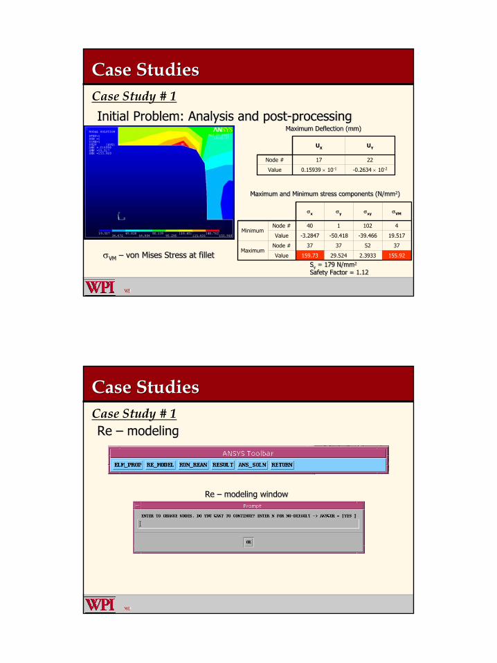
Case StudiesCase StudiesCase Study # 1Initial Problem: Analysis and post-processingInitial Problem: Analysis and postInitial Problem: Analysis and post--processingprocessing

σVM – von Mises Stress at filletσσVMVM –– von Mises Stress at filletvon Mises Stress at fillet

Maximum Deflection (mm)Maximum Deflection (mm)Maximum Deflection (mm)

-0.2634 × 10-20.15939 × 10-1Value

2217Node #

UYUX

Maximum and Minimum stress components (N/mm2)Maximum and Minimum stress components (N/mmMaximum and Minimum stress components (N/mm22))

155.922.393329.524159.73Value

37523737Node #Maximum

19.517-39.466-50.418-3.2847Value

4102140Node #Minimum

σVMσxyσyσx

Sy = 179 N/mm2

Safety Factor = 1.12SSyy = 179 N/mm= 179 N/mm22

Safety Factor = 1.12Safety Factor = 1.12

Case StudiesCase StudiesCase Study # 1Re – modelingRe Re –– modelingmodeling

Re – modeling windowRe Re –– modeling windowmodeling window

Case StudiesCase StudiesCase Study # 1Redesign Option # 1: Plate with Circular HoleRedesign Option # 1: Plate with Circular HoleRedesign Option # 1: Plate with Circular Hole

Case StudiesCase StudiesCase Study # 1Reanalysis ResultsReanalysis ResultsReanalysis Results

Ux – DisplacementUUxx –– DisplacementDisplacement σx – Normal Stress at Filletσσxx –– Normal Stress at FilletNormal Stress at Fillet

Case StudiesCase StudiesCase Study # 1Reanalysis ResultsReanalysis ResultsReanalysis Results

Maximum Deflection (mm)Maximum Deflection (mm)Maximum Deflection (mm)

-0.25617 × 10-20.1583 × 10-1Value

2217Node #

UYUX

Maximum and Minimum stress components (N/mm2)Maximum and Minimum stress components (N/mmMaximum and Minimum stress components (N/mm22))

167.184.054527.045179.03Value

321083232Node #Maximum

20.186-24.293-54.329-3.9486Value

3111Node #Minimum

σvMσxyσyσx

Sy = 179 N/mm2

Safety Factor = 1.00SSyy = 179 N/mm= 179 N/mm22

Safety Factor = 1.00Safety Factor = 1.00

Case StudiesCase StudiesCase Study # 1Reanalysis ResultsReanalysis ResultsReanalysis Results

171717171717-Node #

0.158390.158300.158300.158240.157440.158290.15518ValueMaximum Displacement

×10-1 mm

323232323732-Node #

167.61167.92167.18159.11196.58164.40183.584ValueMaximum σVM

N/mm2

323232323732-Node #

180180.25179.03169.19200.25176.33183.584ValueMaximum σx

N/mm2

RBV – 5RBV – 4RBV – 3RBV – 2RBV – 1

ReanalysisANSYS Direct

AnalysisTheoretical

RBV – Number of Reduced Basis Vectors used for ReanalysisRBV RBV –– Number of Reduced Basis Vectors used for ReanalysisNumber of Reduced Basis Vectors used for Reanalysis

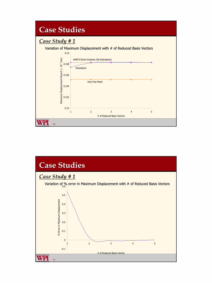
Case StudiesCase StudiesCase Study # 1

Variation of Maximum Displacement with # of Reduced Basis VectorsVariation of Maximum Displacement with # of Reduced Basis VectorVariation of Maximum Displacement with # of Reduced Basis Vectorss

0.15

0.152

0.154

0.156

0.158

0.16

1 2 3 4 5

# of Reduced Basis Vectors

Max

imum

Dis

plac

emen

t R

esul

t ( ×

10-1

mm

)ANSYS Direct Analysis (No Reanalysis)

Reanalysis

Very Fine Mesh

Case StudiesCase StudiesCase Study # 1

Variation of % error in Maximum Displacement with # of Reduced Basis VectorsVariation of % error in Maximum Displacement with # of Reduced BVariation of % error in Maximum Displacement with # of Reduced Basis Vectorsasis Vectors

-0.1

0

0.1

0.2

0.3

0.4

0.5

0.6

1 2 3 4 5

# of Reduced Basis Vector

% E

rror

in M

axim

um D

ispl

acem

ent

Case StudiesCase StudiesCase Study # 1

Variation of Maximum Normal Stress (σx) with # of Reduced Basis VectorsVariation of Maximum Normal Stress (Variation of Maximum Normal Stress (σσxx) with # of Reduced Basis Vectors) with # of Reduced Basis Vectors

160

170

180

190

200

210

1 2 3 4 5

# of Reduced Basis Vectors

Max

imum

Str

ess

(σx)

in N

/mm

2

Reanalysis

Theoretical

ANSYS Direct Analysis (No Reanalysis)

Case StudiesCase StudiesCase Study # 1

Variation of Maximum Normal Stress (σx) with # of Reduced Basis VectorsVariation of Maximum Normal Stress (Variation of Maximum Normal Stress (σσxx) with # of Reduced Basis Vectors) with # of Reduced Basis Vectors

-20

-15

-10

-5

0

5

10

15

20

1 2 3 4 5

# of Reduced Basis Vectors

% E

rror

in M

axim

um S

tres

s (σ

x)

Case StudiesCase StudiesCase Study # 1Redesign Option # 2: Plate with Horizontal Elliptical HoleRedesign Option # 2: Plate with Horizontal Elliptical HoleRedesign Option # 2: Plate with Horizontal Elliptical Hole

Case StudiesCase StudiesCase Study # 1Redesign Option # 3: Plate with Vertical Elliptical HoleRedesign Option # 3: Plate with Vertical Elliptical HoleRedesign Option # 3: Plate with Vertical Elliptical Hole

Case StudiesCase StudiesCase Study # 1Displacement ResultsDisplacement ResultsDisplacement Results

Plate with horizontal elliptical holePlate with horizontal elliptical holePlate with horizontal elliptical hole Plate with vertical elliptical holePlate with vertical elliptical holePlate with vertical elliptical hole

0.15

0.152

0.154

0.156

0.158

0.16

1 2 3 4 5

# of Reduced Basis Vectors

Max

imum

Dis

plac

emen

t (

× 10

-1 m

m)

Very Fine Mesh

ANSYS Direct Analysis (No Reanalysis)

Reanalysis

0.15

0.154

0.158

0.162

1 2 3 4 5

# of Reduced Basis Vectors

Max

imum

Dis

plac

emen

t R

esul

t ( ×

10-1

mm

)

Very Fine Mesh

Reanalysis

ANSYS Direct Analysis (No Reanalysis)

Case StudiesCase StudiesCase Study # 1Stress ResultsStress ResultsStress Results

Plate with horizontal elliptical holePlate with horizontal elliptical holePlate with horizontal elliptical hole Plate with vertical elliptical holePlate with vertical elliptical holePlate with vertical elliptical hole

100

120

140

160

180

200

220

240

1 2 3 4 5

# of Reduced Basis Vectors

Max

imum

Str

ess

( σx)

in N

/mm

2 Reanalysis

ANSYS Direct Analysis

Theoretical

0

50

100

150

200

250

300

350

1 2 3 4 5

# of Reduced Basis Vectors

Max

imum

Str

ess

(σx)

in N

/mm

2

Theoretical

ANSYS Direct analysis (No Reanalysis)

Reanalysis

Case StudiesCase StudiesCase Study # 1Reanalysis Result ComparisonReanalysis Result ComparisonReanalysis Result Comparison

-0.570.6-1.31.33-11.02Safety Factor

Redesign Options

0.15958

274.29

298.75

ANSYS Direct

Analysis

0.0063

2.44

2.72

% Error

0.15829

164.40

176.33

ANSYS Direct

Analysis

0.0130.159560.157050.157040.00630.15830Displacement

Ux(× 10-1 mm)

5.25288.70129.53126.441.69167.18σVM N/mm2

5.19314.27137.94134.281.53179.03σxN/mm2

% ErrorReanalysisReanalysisANSYS Direct

Analysis% ErrorReanalysis

# 3: Vertical Ellipse# 2: Horizontal Ellipse# 1: Circular HoleMaximum Quantities

Case StudiesCase StudiesCase Study # 1Conclusion:Conclusion:Conclusion:

1. Three different geometries explored2. Horizontal elliptical hole shows lower stress

results3. The displacement results are very accurate

for three reduced basis vectors4. Stress results are near to the ANSYS Direct

Analysis results5. Accuracy increases as the number of reduced

basis vectors is increased

1.1. Three different geometries exploredThree different geometries explored2.2. Horizontal elliptical hole shows lower stress Horizontal elliptical hole shows lower stress

resultsresults3.3. The displacement results are very accurate The displacement results are very accurate

for three reduced basis vectorsfor three reduced basis vectors4.4. Stress results are near to the ANSYS Direct Stress results are near to the ANSYS Direct

Analysis resultsAnalysis results5.5. Accuracy increases as the number of reduced Accuracy increases as the number of reduced

basis vectors is increasedbasis vectors is increased

Case StudiesCase StudiesCase Study # 2 : Optimal Free-Form Fillet under Tension

Initial Problem:Initial Problem:Initial Problem: Mesh Characteristics:125 Four-node Quad Elements156 Nodes2 DOF/node312 Total DOF

Element and Material Properties:PLANE42 – Four node quadPlane Stress with thicknessPoisson’s ratio – 0.3 Young’s Modulus – 72400 N/mm2

Thickness – 1 mma/b = 2l/h = 1

Case StudiesCase StudiesCase Study # 2

Initial Problem: FEM Mesh used by Waldman [4.2]Initial Problem: FEM Mesh used by Waldman [4.2]Initial Problem: FEM Mesh used by Waldman [4.2]

Case StudiesCase StudiesCase Study # 2

Initial Problem: FE ModelInitial Problem: FE ModelInitial Problem: FE Model

Case StudiesCase StudiesCase Study # 2

Initial Problem: FE ModelInitial Problem: FE ModelInitial Problem: FE Model Mesh Characteristics:125 Four-node Quad Elements156 Nodes2 DOF/node312 Total DOF

Element and Material Properties:PLANE42 – Four node quadPlane Stress with thicknessPoisson’s ratio – 0.3 Young’s Modulus – 72400 N/mm2

Thickness – 1 mma/b = 2l/h = 1

Case StudiesCase StudiesCase Study # 2

Initial Problem: Analysis and Post-processingInitial Problem: Analysis and PostInitial Problem: Analysis and Post--processingprocessing

σVM – von Mises StressσσVMVM –– von Mises Stressvon Mises Stress

-0.36526×10-40.17647×10-3Value

112Node #

UYUX

Maximum Deflection (mm)Maximum Deflection (mm)Maximum Deflection (mm)

Maximum and Minimum stress components (N/mm2)Maximum and Minimum stress components (N/mmMaximum and Minimum stress components (N/mm22))

1.51670.104×10-10.29361.5184Value

3213232Node #Maximum

0.1414×10-1-0.3643-0.1735-0.154×10-1Value

52511152Node #Minimum

σvMσxyσyσx

Case StudiesCase StudiesCase Study # 2

Redesign Option # 1: Optimum Shape of filletRedesign Option # 1: Optimum Shape of filletRedesign Option # 1: Optimum Shape of fillet

Ux – DisplacementUUxx –– DisplacementDisplacement σx – Normal Stressσσxx –– Normal StressNormal Stress

Case StudiesCase StudiesCase Study # 2

σVM – von Mises StressσσVMVM –– von Mises Stressvon Mises Stress

-0.35971×10-40.18524×10-3Value

127Node #

UYUX

1.2180.144×10-10.3121.2241Value

4914649Node #Maximum

0.544×10-2-0.372-0.186-0.41×10-1Value

64461058Node #Minimum

σVMσxyσyσx

Maximum Deflection (mm)Maximum Deflection (mm)Maximum Deflection (mm)

Maximum and Minimum stress components (N/mm2)Maximum and Minimum stress components (N/mmMaximum and Minimum stress components (N/mm22))

Redesign Option # 1: ResultsRedesign Option # 1: ResultsRedesign Option # 1: Results

Case StudiesCase StudiesCase Study # 2

0.18

0.181

0.182

0.183

0.184

0.185

0.186

0.187

1 2 3 4 5

# of Reduced Basis Vectors

Max

imum

Dis

plac

emen

t (

10-3

mm

)

ANSYS Direct Analysis

Very Fine Mesh

Reanalysis

1.15

1.35

1.55

1 2 3 4 5

# of Reduced Basis Vectors

Max

imum

σx

in N

/mm

2

Results [4.2]

ANSYS Direct Analysis

Reanalysis

Redesign Option # 1: Displacement and StressRedesign Option # 1: Displacement and StressRedesign Option # 1: Displacement and Stress

Case StudiesCase StudiesCase Study # 2

Redesign Option # 2 and 3:Redesign Option # 2 and 3:Redesign Option # 2 and 3:

Case StudiesCase StudiesCase Study # 2

Reanalysis Results:Reanalysis Results:Reanalysis Results:

0.17543

1.2727

1.288

ANSYS Direct

Analysis

# 3: Two Circular Arcs

0.17517

1.2749

1.2913

Reanalysis

0.19

1.1

0.29

% Error

0.15

0.17

0.25

% Error

0.18024

1.4096

1.3892

Reanalysis

0.18058

1.3932

1.3852

ANSYS Direct

Analysis

# 2: Circular Arc Fillet

0.20

0.44

0.84

% Error

0.18524

1.2180

1.2241

Reanalysis

0.18562

1.2127

1.2138

ANSYS Direct

Analysis

# 1: Free-form Fillet

Redesign Options

Ux(× 10-3 mm)

σVMN/mm2

σxN/mm2

Maximum Quantities

Case StudiesCase StudiesCase Study # 3 : Support Bracket Redesign

Initial Problem: FE ModelInitial Problem: FE ModelInitial Problem: FE Model

Case StudiesCase StudiesCase Study # 3 : Support Bracket Redesign

Initial Problem: FE ModelInitial Problem: FE ModelInitial Problem: FE ModelMesh Characteristics:349 Four-node Quad Elements415 Nodes2 DOF/node830 Total DOF

Element and Material Properties:Material: Stainless Steel Type 302PLANE42 – Four node quadPlane Stress with thicknessPoisson’s ratio – 0.28 Young’s Modulus – 206.8 GPaThickness – 1 mmYield Stress (Sy)– 276 N/mm2

Case StudiesCase StudiesCase Study # 3 : Support Bracket Redesign

Initial Problem: Analysis and post-processingInitial Problem: Analysis and postInitial Problem: Analysis and post--processingprocessing

USUM – Displacement Vector SumUUSUMSUM –– Displacement Vector SumDisplacement Vector Sum σx – Normal Stressσσxx –– Normal StressNormal Stress

Case StudiesCase StudiesCase Study # 3 : Support Bracket Redesign

Initial Problem: Analysis and post-processingInitial Problem: Analysis and postInitial Problem: Analysis and post--processingprocessing

σVM – von Mises StressσσVMVM –– von Mises Stressvon Mises Stress

Maximum Deflection (mm)Maximum Deflection (mm)Maximum Deflection (mm)

Maximum and Minimum stress components (N/mm2)Maximum and Minimum stress components (N/mmMaximum and Minimum stress components (N/mm22))

-0.9685 × 10-10.18767 × 10-1Value

4343Node #

UYUX

152.5933.69019.739108.30Value

517919256Node #Maximum

0.27448-62.146-121.55-129.61Value

1765432Node #Minimum

σvMσxyσyσx

Sy = 276 N/mm2

Safety Factor = 1.8SSyy = 276 N/mm= 276 N/mm22

Safety Factor = 1.8Safety Factor = 1.8

Case StudiesCase StudiesCase Study # 3 : Support Bracket RedesignRedesign Option # 1: Optimum thicknessRedesign Option # 1: Optimum thicknessRedesign Option # 1: Optimum thickness

For the support under point load, the maximum bending stress is,For the support under point load, the maximum bending stress is,For the support under point load, the maximum bending stress is,

312

12)(maxhb

hxPIyM

x ⋅⋅

⋅⋅=

⋅=σ

maxxσ

Phb

= Maximum bending stress= Maximum bending stress= Maximum bending stress

= Applied Load= Applied Load= Applied Load

= Height= Height= Height

= Width = thickness for plane stress problem

= Width = thickness for plane = Width = thickness for plane stress problemstress problemxPh

x⋅

⋅= max

6σ

Thus,Thus,Thus,

Case StudiesCase StudiesCase Study # 3 : Support Bracket RedesignRedesign Option # 1: Optimum ThicknessRedesign Option # 1: Optimum ThicknessRedesign Option # 1: Optimum Thickness

Mesh Characteristics:349 Four-node Quad Elements415 Nodes2 DOF/node830 Total DOF

Element and Material Properties:Material: Stainless Steel Type 302PLANE42 – Four node quadPlane Stress with thicknessPoisson’s ratio – 0.28 Young’s Modulus – 206.8 GPaThickness – 1 mmYield Stress (Sy)– 276 N/mm2

Case StudiesCase StudiesCase Study # 3 : Support Bracket RedesignRedesign Option # 1: ResultsRedesign Option # 1: ResultsRedesign Option # 1: Results

USUM – Displacement Vector SumUUSUMSUM –– Displacement Vector SumDisplacement Vector Sum σx – Normal Stressσσxx –– Normal StressNormal Stress

Case StudiesCase StudiesCase Study # 3 : Support Bracket RedesignRedesign Option # 1: ResultsRedesign Option # 1: ResultsRedesign Option # 1: Results

-0.74779 × 10-10.15196 × 10-1Value

4343Node #

UYUX

Maximum Deflection (mm)Maximum Deflection (mm)Maximum Deflection (mm)

Maximum and Minimum stress components (N/mm2)Maximum and Minimum stress components (N/mmMaximum and Minimum stress components (N/mm22))

159.4033.47719.54696.196Value

517919251Node #Maximum

0.2528-62.044-124.86-142.37Value

1765432Node #Minimum

σVMσxyσyσx

Sy = 276 N/mm2

Safety Factor = 1.7SSyy = 276 N/mm= 276 N/mm22

Safety Factor = 1.7Safety Factor = 1.7

Case StudiesCase StudiesCase Study # 3 : Support Bracket Redesign

Redesign Option # 2 and 3: Increasing the Fillet RadiusRedesign Option # 2 and 3: Increasing the Fillet RadiusRedesign Option # 2 and 3: Increasing the Fillet Radius

Case StudiesCase StudiesCase Study # 3 : Support Bracket RedesignReanalysis ResultsReanalysis ResultsReanalysis Results

0.6652

2.3

118.40

-118.58

ANSYS Direct

Analysis

# 3: Fillet Radius 7.5 mm

Design Options

0.028

2.7

0.33

% Error

0.7083

2.2

126.96

-122.11

Reanalysis

0.19

2.8

2.9

% Error

0.66394

2.3

121.79

-122.03

Reanalysis

-0.7085

2.2

123.55

-121.71

ANSYS Direct

Analysis

# 2: Fillet Radius 5 mm

0.015

4.6

2.59

% Error

-0.74779

1.7

159.40

-142.37

Reanalysis

-0.7479

1.8

152.39

-138.77

ANSYS Direct

Analysis

# 1: Optimum Shape of Taper

-0.9685

1.8

152.59

-129.61

ANSYS Direct Analysis

Initial Design:Fillet Radius

2.5 mm

UY(× 10-1 mm)

Safety Factor

σVMN/mm2

Compressive σx

N/mm2

Maximum Quantities

Cost AnalysisCost Analysis1m 10 KutU ∆n 20n 2m 20 KutU ∆n 30n ][ 21 sB KuB3m RBB KuKu )( FuF BR RR y yB ( )2 4 3 3 12 18m n n m m + + + + +

Total number of multiplications and divisions in case of Direct Analysis using Cholesky Decomposition MethodTotal number of multiplications and divisions in case of Direct Total number of multiplications and divisions in case of Direct Analysis using Analysis using Cholesky Decomposition MethodCholesky Decomposition Method

+ 2

3

6nn

Total number of multiplications and divisions in case of Combined Approximation Reanalysis MethodTotal number of multiplications and divisions in case of CombineTotal number of multiplications and divisions in case of Combined Approximation d Approximation Reanalysis MethodReanalysis Method

( )3 2 22 4 3 3 12 18m n n m m + + + + + where,m = Total number of DOFs changedn = Total number of DOFs of the systemSince m << n

where,where,m = Total number of DOFs changedm = Total number of DOFs changedn = Total number of DOFs of the systemn = Total number of DOFs of the systemSince m << nSince m << n

nnm 342 23 ++

Total number of multiplications and divisions in case of Combined Approximation Reanalysis MethodTotal number of multiplications and divisions in case of CombineTotal number of multiplications and divisions in case of Combined Approximation d Approximation Reanalysis MethodReanalysis Method

Cost AnalysisCost Analysis1m 10 utUn 20n 2m 20 utUn 30n ][ 21 sB KuB3m RBB KuKu )( FuF BR RR y yB ( )2 4 3 3 12 18m n n m m + + + + +

For Reanalysis method to be faster than the Direct analysis methodFor Reanalysis method to be faster than the Direct analysis methFor Reanalysis method to be faster than the Direct analysis methodod

nnm 342 23 ++ should be less thanshould be less thanshould be less than

+ 2

3

6nn

23

23

6342 nnnnm +≤++

nnnm 336

2 23

3 −−≤

4368.0≤nm

Yielding,Yielding,Yielding,

CA method is most efficient when the coordinates of less than 43% of node out of total number of nodes is changed.CA method is most efficient when the coordinates of less than 43CA method is most efficient when the coordinates of less than 43% of node % of node out of total number of nodes is changed.out of total number of nodes is changed.

Total # of DOFs changedTotal # of DOFs changedTotal # of DOFs changed

Total # of DOFs of the systemTotal # of DOFs of the systemTotal # of DOFs of the system===

ConclusionConclusion

Reanalysis method coupled with the design process offers many advantages for improving the design

CA method can be effectively used in reanalysis

Three reduced basis vectors are sufficient for better accuracy for displacement and stress

Reanalysis algorithm using CA method is more efficient up to 43 % of change in node locations

Future WorkFuture Work

Improved ANSYS Output EnvironmentUsing Combined Approximation Method for Change in # of DOF3-Dimensional ProblemsFactor of Safety PlotsFatigue Analysis PlotsBoundary Elements