graphing calculator - sharp global the unique features of the sharp graphing calculator. this book,...
TRANSCRIPT
A P P L Y I N G
U S I N G T H E
E L - 9 6 0 0D A V I D P . L A W R E N C E
STATISTICS
SHARP
Graphing Calculator
SHARP STAT COVER 02.2.19 11:09 AM Page 3
STATISTICS USING THE SHARP EL-9600 i
ApplyingSTATISTICS
using theSHARP EL-9600
GRAPHING CALCULATOR
David P. LawrenceSouthwestern Oklahoma State University
This Teaching Resource has been developed specifically for use with theSharp EL-9600 graphing calculator. The goal for preparing this book wasto provide mathematics educators with quality teaching materials thatutilize the unique features of the Sharp graphing calculator.
This book, along with the Sharp graphing calculator, offers you and yourstudents 10 classroom-tested, topic-specific lessons that build skills.Each lesson includes Introducing the Topic, Calculator Operations, Methodof Teaching, explanations for Using Blackline Masters, For Discussion, and Additional Problems to solve. Conveniently located in the back of the book are 34 reproducible Blackline Masters. You’ll find them ideal for creating handouts, overhead transparencies, or to use as studentactivity worksheets for extra practice. Solutions to the Activities are also included.
We hope you enjoy using this resource book and the Sharp EL-9600 graphing calculator in your classroom.
Other books are also available:
Applying TRIGONOMETRY using the SHARP EL-9600 Graphing CalculatorApplying PRE-ALGEBRA and ALGEBRA using the SHARP EL-9600 Graphing CalculatorApplying PRE-CALCULUS and CALCULUS using the SHARP EL-9600 Graphing CalculatorGraphing Calculators: Quick & Easy! The SHARP EL-9600
ii STATISTICS USING THE SHARP EL-9600
Dedicated to members of First Baptist Church, Okarche, Oklahoma
Special thanks to Ms. Marina Ramirez and Ms. Melanie Drozdowski for their comments
and suggestions.
Developed and prepared by Pencil Point Studio.
Copyright © 1998 by Sharp Electronics Corporation.All rights reserved. This publication may not be reproduced, stored in a retrieval system, or transmitted in any form or by any means, electronic, mechanical, photocopying, recording, or otherwise without written permission.
The blackline masters in this publication are designed to be used with appropriate duplicating equipment to reproduce for classroom use.
First printed in the United States of America in 1998.
STATISTICS USING THE SHARP EL-9600 iii
CONTENTS
CHAPTER TOPIC PAGE
1 Creation of a One-Variable Data Set 1
2 Numerical Description of a One-Variable Data Set 6
3 Histogram Representation of a One-Variable Data Set 11
4 Other Graphical Portrayals of a One-Variable Data Set 16
5 Creation of a Two-Variable Data Set 21
6 Numerical Description of a Two-Variable Data Set 26
7 Graphical Portrayal of a Two-Variable Data Set 32
8 Linear Regressions 38
9 Other Regressions and Model of "Best Fit" 44
10 Statistical Tests 49
Blackline Masters 55
Solutions to the Activities 90
Creation of a One-Variable Data Set/STATISTICS USING THE SHARP EL-9600 1
CREATION OF A ONE-VARIABLE DATA SET
Chapter one
Introducing the TopicIn this chapter, you and your students will learn how to delete an old data set,
create a one-variable data set, save and retrieve data.
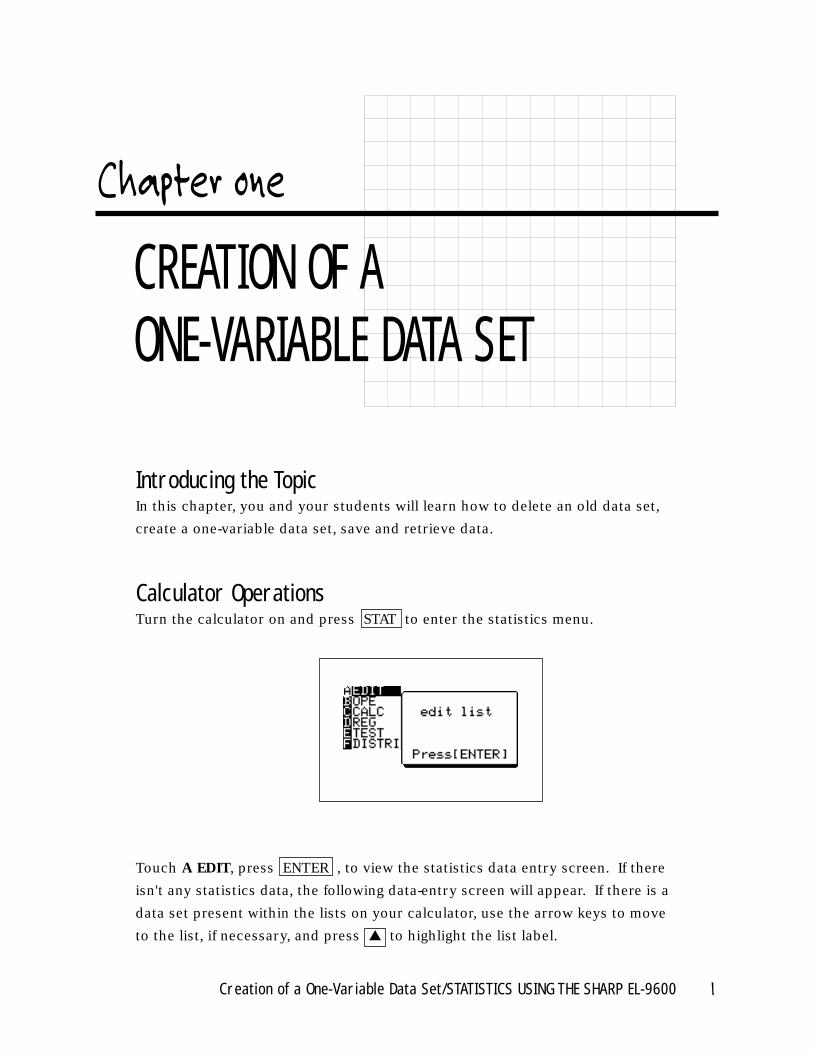
Calculator OperationsTurn the calculator on and press STAT to enter the statistics menu.
Touch A EDIT, press ENTER , to view the statistics data entry screen. If there
isn't any statistics data, the following data-entry screen will appear. If there is a
data set present within the lists on your calculator, use the arrow keys to move
to the list, if necessary, and press ▲ to highlight the list label.
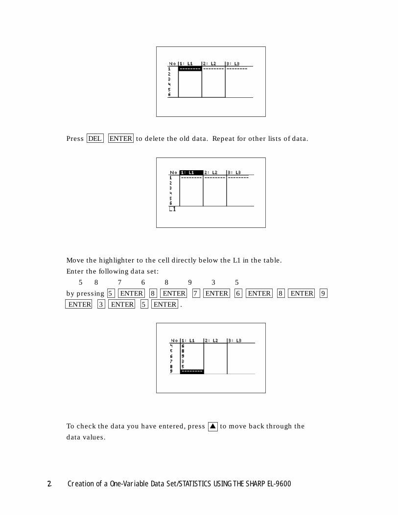
Press DEL ENTER to delete the old data. Repeat for other lists of data.
Move the highlighter to the cell directly below the L1 in the table.
Enter the following data set:
5 8 7 6 8 9 3 5
by pressing 5 ENTER 8 ENTER 7 ENTER 6 ENTER 8 ENTER 9
ENTER 3 ENTER 5 ENTER .
To check the data you have entered, press ▲ to move back through the
data values.
2 Creation of a One-Variable Data Set/STATISTICS USING THE SHARP EL-9600
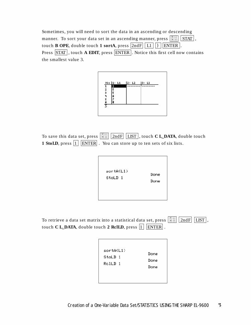
Sometimes, you will need to sort the data in an ascending or descending
manner. To sort your data set in an ascending manner, press STAT ,
touch B OPE, double touch 1 sortA, press 2ndF L1 ) ENTER .
Press STAT , touch A EDIT, press ENTER . Notice this first cell now contains
the smallest value 3.
To save this data set, press 2ndF LIST , touch C L_DATA, double touch
1 StoLD, press 1 ENTER . You can store up to ten sets of six lists.
To retrieve a data set matrix into a statistical data set, press 2ndF LIST ,
touch C L_DATA, double touch 2 RclLD, press 1 ENTER .
Creation of a One-Variable Data Set/STATISTICS USING THE SHARP EL-9600 3
×+ –
÷
×+ –
÷
×+ –
÷
Method of TeachingUse the Blackline Masters 1.1 and 1.2 to create overheads for entering one
variable data sets that are non-weighted and weighted. Go over in detail how
to save data sets to and retrieve data sets.
Next, use the Blackline Masters 1.3 to create worksheets for the students.
Have the students enter and save the non-weighted and weighted data
sets for one variable. Use the topics For Discussion to supplement the
worksheets.
Using Blackline Master 1.2The creation of a non-weighted one-variable data set discussed above under
Calculator Operations is presented on Blackline Master 1.1. The entering of a
weighted one-variable data set appears on Blackline Master 1.2.
Turn the calculator on and press STAT to enter the statistics menu.
Touch A EDIT, press ENTER , to view the statistics data entry screen. Remove
old data by using the arrow keys to move to the list of data, and press ▲ to
highlight the list label. Press DEL ENTER to delete the old data. Repeat for
other lists of data.
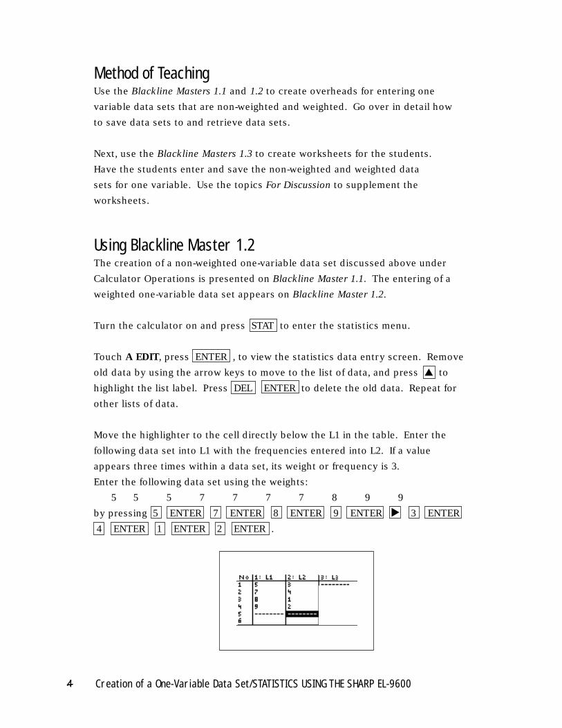
Move the highlighter to the cell directly below the L1 in the table. Enter the
following data set into L1 with the frequencies entered into L2. If a value
appears three times within a data set, its weight or frequency is 3.
Enter the following data set using the weights:
5 5 5 7 7 7 7 8 9 9
by pressing 5 ENTER 7 ENTER 8 ENTER 9 ENTER 3 ENTER
4 ENTER 1 ENTER 2 ENTER .
4 Creation of a One-Variable Data Set/STATISTICS USING THE SHARP EL-9600
▼
To save this data set, press 2ndF LIST , touch C L_DATA,
double touch 1 StoLD, press 2 ENTER .
For DiscussionYou and your students can discuss:
1. Why you would want to sort in an ascending manner?
2. Why you would want to sort in a descending manner?
3. Why you would want to save a data set?
Creation of a One-Variable Data Set/STATISTICS USING THE SHARP EL-9600 5
×+ –
÷
Introducing the TopicIn this chapter, you and your students will learn how to use the Sharp graphing
calculator to find the numerical descriptions of a one-variable data set.
Calculator OperationsTurn the calculator on and press STAT to enter the statistics menu.
Touch A EDIT, press ENTER , to view the statistics data entry screen. If there
is a data set present within the lists on your calculator, use the arrow keys to
move to the list, if necessary, and press ▲ to highlight the list label. Press
DEL ENTER to delete the old data. Repeat for other lists of data.
Move the highlighter to the cell directly below the L1 in the table.
Enter the following data set:
25 32 28 33 31 27 40 38 29 30
Use the non-weighted format for entering the data since no entry occurs more
than once. Refer to Chapter 1 for information on how to enter a non-weighted
one-variable data set.
6 Numerical Description of a One-Variable Data Set/STATISTICS USING THE SHARP EL-9600
NUMERICAL DESCRIPTION OF A0NE-VARIABLE DATA SET
Chapter two
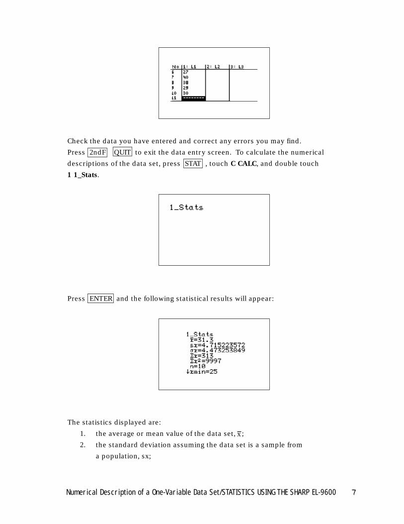
Check the data you have entered and correct any errors you may find.
Press 2ndF QUIT to exit the data entry screen. To calculate the numerical
descriptions of the data set, press STAT , touch C CALC, and double touch
1 1_Stats.
Press ENTER and the following statistical results will appear:
The statistics displayed are:
1. the average or mean value of the data set, ;
2. the standard deviation assuming the data set is a sample from
a population, sx;
Numerical Description of a One-Variable Data Set/STATISTICS USING THE SHARP EL-9600 7
x
3. the standard deviation assuming the data set represents the
entire population, σx;
4. the sum of the data values, ∑x;
5. the sum of the squared data values, ∑x2;
6. the number of values in the data set, n;
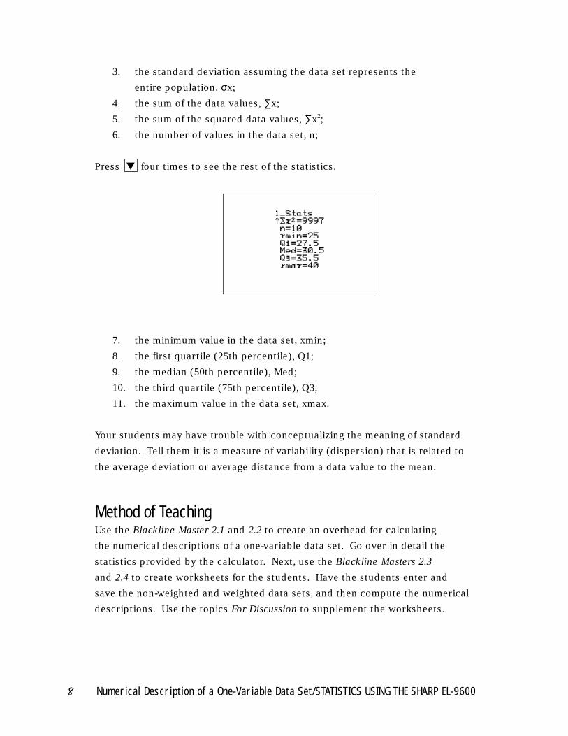
Press ▼ four times to see the rest of the statistics.
7. the minimum value in the data set, xmin;
8. the first quartile (25th percentile), Q1;
9. the median (50th percentile), Med;
10. the third quartile (75th percentile), Q3;
11. the maximum value in the data set, xmax.
Your students may have trouble with conceptualizing the meaning of standard
deviation. Tell them it is a measure of variability (dispersion) that is related to
the average deviation or average distance from a data value to the mean.
Method of TeachingUse the Blackline Master 2.1 and 2.2 to create an overhead for calculating
the numerical descriptions of a one-variable data set. Go over in detail the
statistics provided by the calculator. Next, use the Blackline Masters 2.3
and 2.4 to create worksheets for the students. Have the students enter and
save the non-weighted and weighted data sets, and then compute the numerical
descriptions. Use the topics For Discussion to supplement the worksheets.
8 Numerical Description of a One-Variable Data Set/STATISTICS USING THE SHARP EL-9600
Using Blackline Master 2.2Calculation of one-variable statistics for a non-weighted data set is covered
above under Calculator Operations and is presented on Blackline Master 2.1.
Turn the calculator on and press STAT to enter the statistics menu. Touch
A EDIT, press ENTER , to view the statistics data entry screen. If there is a
data set present within the lists on your calculator, use the arrow keys to
move to the list, if necessary, press ▲ to highlight the list label. Press DEL
ENTER to delete the old data. Repeat for other lists of data.
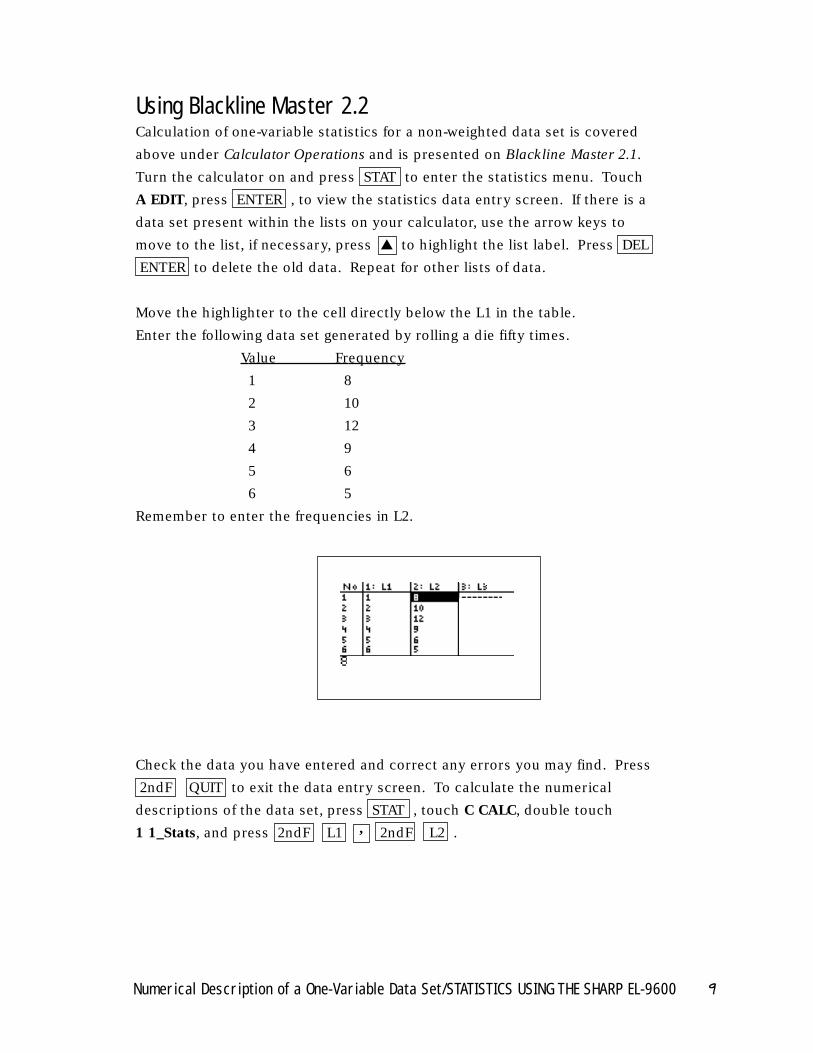
Move the highlighter to the cell directly below the L1 in the table.
Enter the following data set generated by rolling a die fifty times.
Value Frequency
1 8
2 10
3 12
4 9
5 6
6 5
Remember to enter the frequencies in L2.
Check the data you have entered and correct any errors you may find. Press
2ndF QUIT to exit the data entry screen. To calculate the numerical
descriptions of the data set, press STAT , touch C CALC, double touch
1 1_Stats, and press 2ndF L1 , 2ndF L2 .
Numerical Description of a One-Variable Data Set/STATISTICS USING THE SHARP EL-9600 9
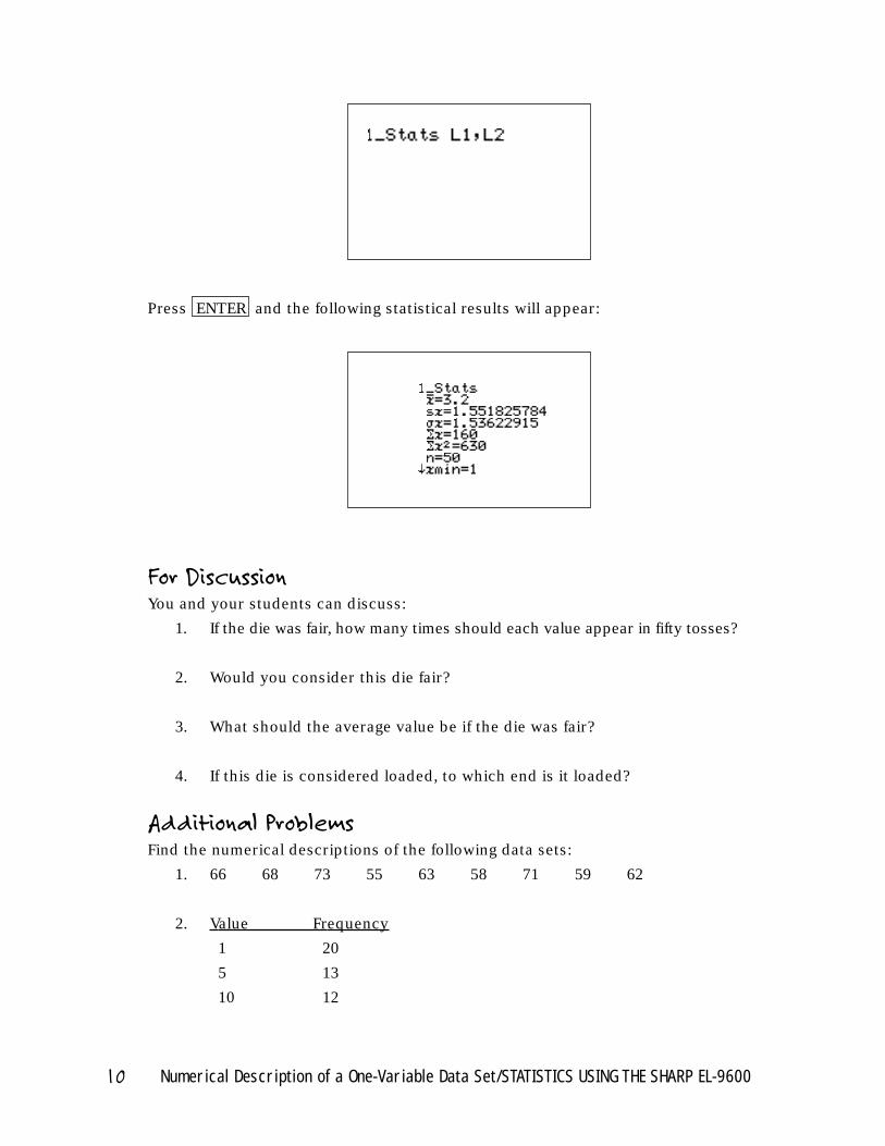
Press ENTER and the following statistical results will appear:
For DiscussionYou and your students can discuss:
1. If the die was fair, how many times should each value appear in fifty tosses?
2. Would you consider this die fair?
3. What should the average value be if the die was fair?
4. If this die is considered loaded, to which end is it loaded?
Additional ProblemsFind the numerical descriptions of the following data sets:
1. 66 68 73 55 63 58 71 59 62
2. Value Frequency
1 20
5 13
10 12
10 Numerical Description of a One-Variable Data Set/STATISTICS USING THE SHARP EL-9600
Introducing the TopicIn this chapter, you and your students will learn how to use the Sharp graphing
calculator to represent a one-variable data set as a histogram. Typically, a
histogram is represented on a horizontal (x) axis scaled according to the data,
with a vertical (y) axis scaled according to the data's frequency individually
(discrete) or within an interval (continuous). In each case, a bar is drawn with
its width determined by an interval on the x-axis, and its height determined by
the frequency of data within the interval.
Normally, you should seek between 5 and 7 intervals or bars; however, there
will be times you will need more or less intervals. Interval widths can be
determined logically or mathematically. Remember, the object of viewing a
histogram is to obtain or portray characteristics of the data's distribution,
therefore the number of intervals may vary.
Calculator OperationsTurn the calculator on and press STAT to enter the statistics menu.
Touch A EDIT, press ENTER , to view the statistics data entry screen.
If there is a data set present within the lists on your calculator, use the
Histogram Representation of a One-Variable Data Set/STATISTICS USING THE SHARP EL-9600 11
HISTOGRAM REPRESENTATION OF A ONE-VARIABLE DATA SET
Chapter three
arrow keys to move to the list, if necessary, and press ▲ to highlight the list
label. Press DEL ENTER to delete the old data. Repeat for other lists of data.
Move the highlighter to the cell directly below the L1 in the table and enter the
following data set:
15 28 17 36 38 19 13 25 27 41
by pressing 1 5 ENTER 2 8 ENTER 1 7 ENTER 3 6 ENTER
3 8 ENTER 1 9 ENTER 1 3 ENTER 2 5 ENTER 2 7
ENTER 4 1 ENTER .
Check the data you have entered by pressing ▲ to move back through the data.
Save this data set by pressing 2ndF LIST , touch C L_DATA, double
touch 1 StoLD, press 1 ENTER .
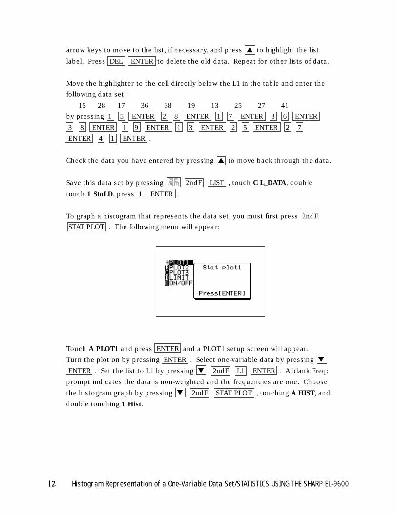
To graph a histogram that represents the data set, you must first press 2ndF
STAT PLOT . The following menu will appear:
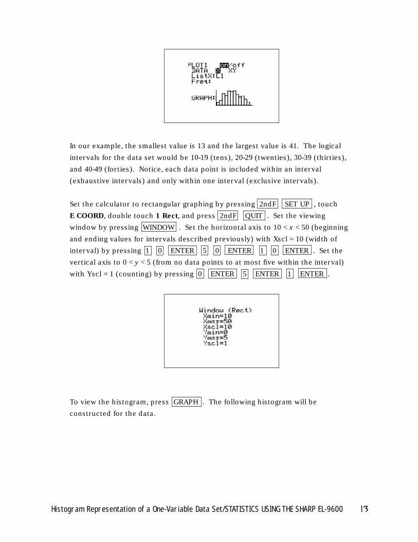
Touch A PLOT1 and press ENTER and a PLOT1 setup screen will appear.
Turn the plot on by pressing ENTER . Select one-variable data by pressing ▼
ENTER . Set the list to L1 by pressing ▼ 2ndF L1 ENTER . A blank Freq:
prompt indicates the data is non-weighted and the frequencies are one. Choose
the histogram graph by pressing ▼ 2ndF STAT PLOT , touching A HIST, and
double touching 1 Hist.
12 Histogram Representation of a One-Variable Data Set/STATISTICS USING THE SHARP EL-9600
×+ –
÷
In our example, the smallest value is 13 and the largest value is 41. The logical
intervals for the data set would be 10-19 (tens), 20-29 (twenties), 30-39 (thirties),
and 40-49 (forties). Notice, each data point is included within an interval
(exhaustive intervals) and only within one interval (exclusive intervals).
Set the calculator to rectangular graphing by pressing 2ndF SET UP , touch
E COORD, double touch 1 Rect, and press 2ndF QUIT . Set the viewing
window by pressing WINDOW . Set the horizontal axis to 10 < x < 50 (beginning
and ending values for intervals described previously) with Xscl = 10 (width of
interval) by pressing 1 0 ENTER 5 0 ENTER 1 0 ENTER . Set the
vertical axis to 0 < y < 5 (from no data points to at most five within the interval)
with Yscl = 1 (counting) by pressing 0 ENTER 5 ENTER 1 ENTER .
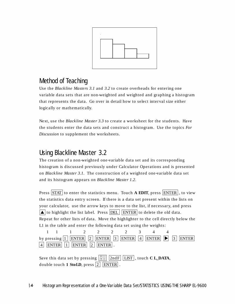
To view the histogram, press GRAPH . The following histogram will be
constructed for the data.
Histogram Representation of a One-Variable Data Set/STATISTICS USING THE SHARP EL-9600 13
Method of TeachingUse the Blackline Masters 3.1 and 3.2 to create overheads for entering one
variable data sets that are non-weighted and weighted and graphing a histogram
that represents the data. Go over in detail how to select interval size either
logically or mathematically.
Next, use the Blackline Master 3.3 to create a worksheet for the students. Have
the students enter the data sets and construct a histogram. Use the topics For
Discussion to supplement the worksheets.
Using Blackline Master 3.2The creation of a non-weighted one-variable data set and its corresponding
histogram is discussed previously under Calculator Operations and is presented
on Blackline Master 3.1. The construction of a weighted one-variable data set
and its histogram appears on Blackline Master 1.2.
Press STAT to enter the statistics menu. Touch A EDIT, press ENTER , to view
the statistics data entry screen. If there is a data set present within the lists on
your calculator, use the arrow keys to move to the list, if necessary, and press
▲ to highlight the list label. Press DEL ENTER to delete the old data.
Repeat for other lists of data. Move the highlighter to the cell directly below the
L1 in the table and enter the following data set using the weights:
1 1 1 2 2 2 2 3 4 4
by pressing 1 ENTER 2 ENTER 3 ENTER 4 ENTER 3 ENTER
4 ENTER 1 ENTER 2 ENTER .
Save this data set by pressing 2ndF LIST , touch C L_DATA,
double touch 1 StoLD, press 2 ENTER .
14 Histogram Representation of a One-Variable Data Set/STATISTICS USING THE SHARP EL-9600
▼
×+ –
÷
Press 2ndF STAT PLOT , touch A PLOT1, and press ENTER and a PLOT1
setup screen will appear. Turn the plot on by pressing ENTER . Select
one-variable data by pressing ▼ ENTER Set the list to L1 by pressing ▼
2ndF L1 ENTER . Set the frequencies to L2 by pressing 2ndF L2 ENTER .
Choose the histogram graph by pressing 2ndF STAT PLOT , touching A HIST,
and double touching 1 Hist.
In our example, the smallest value is 1 and the largest value is 4. The logical
intervals for the data set would be 1 (0.5 to 1.5), 2 (1.5 to 2.5), 3 (2.5 to 3.5), and
4 (3.5 to 4.5). Notice, the mutually exclusive and exhaustive intervals.
To set this viewing window, press WINDOW and set the horizontal axis to -.5 < x
< 5.5 (one below the smallest endpoint and one above the largest endpoint) with
Xscl = 1 (width of interval) by pressing (–) • 5 ENTER 5 • 5 ENTER
1 ENTER . Next, set the vertical axis to -1 < y < 5 (from one less than no data
points to at most five within the interval, which is one more than the largest
weight) with Yscl = 1 (counting) by pressing (–) 1 ENTER 5 ENTER 1
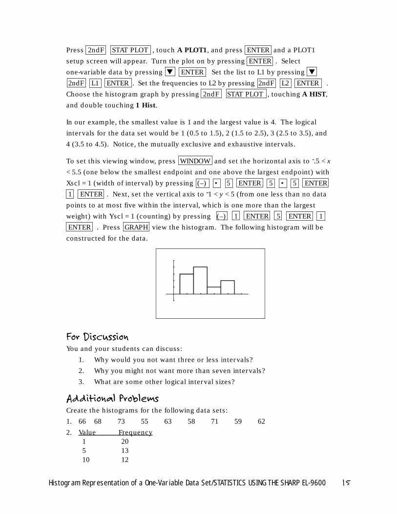
ENTER . Press GRAPH view the histogram. The following histogram will be
constructed for the data.
For DiscussionYou and your students can discuss:
1. Why would you not want three or less intervals?
2. Why you might not want more than seven intervals?
3. What are some other logical interval sizes?
Additional ProblemsCreate the histograms for the following data sets:
1. 66 68 73 55 63 58 71 59 62
2. Value Frequency1 205 1310 12
Histogram Representation of a One-Variable Data Set/STATISTICS USING THE SHARP EL-9600 15
Introducing the TopicIn this chapter, you and your students will learn how to use the Sharp
graphing calculator to represent a one-variable data set with a broken-line
graph (frequency polygon) and a box-and-whisker chart.
Typically, a broken-line graph is represented on a horizontal (x) axis scaled
according to the data, with a vertical (y) axis scaled according to the data's
frequency individually (discrete) or within an interval (continuous). In each case, a
point is plotted at the coordinates (x, frequency) for a discrete distribution or the
coordinates (interval right-point, interval frequency). Lines are then drawn from one
of these points to the next one. Remember, when using intervals, you should seek
between 5 and 7 intervals. Once again, there will be times you will need more or less
intervals. Interval widths can be determined logically or mathematically. Remember,
the object of viewing a broken-line graph is to obtain or portray characteristics of the
data's distribution. Therefore, the number of intervals may vary.
A box-and-whisker chart is a graph that consists of five points of interest. The
25th percentile, 50th percentile, and 75th percentiles are each indicated with a
vertical line. The three vertical lines are then connected together in order to
form a box. Next, vertical lines are extended away from the box to the minimum
and maximum. These are called the whiskers of the chart.
16 Other Graphical Portrayals of a One-Variable Data Set/STATISTICS USING THE SHARP EL-9600
OTHER GRAPHICAL PORTRAYALS OF A ONE-VARIABLE DATA SET
Chapter four
Calculator OperationsTurn the calculator on and press STAT to enter the statistics menu.
Delete old data and enter the following data set for L1:
15 28 17 36 38 19 13 25 27 41
by pressing 1 5 ENTER 2 8 ENTER 1 7 ENTER 3 6 ENTER
3 8 ENTER 1 9 ENTER 1 3 ENTER 2 5 ENTER 2 7 ENTER
4 1 ENTER .
Check the data you have entered by pressing ▲ to move back through the data.
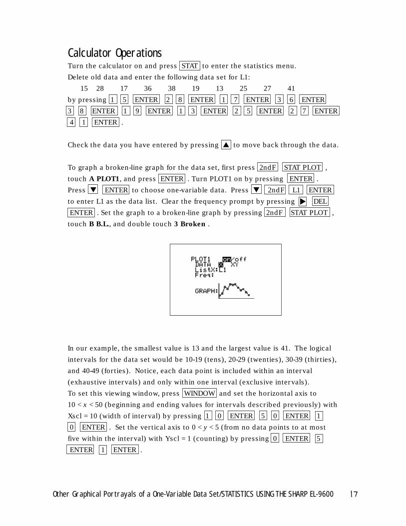
To graph a broken-line graph for the data set, first press 2ndF STAT PLOT ,
touch A PLOT1, and press ENTER . Turn PLOT1 on by pressing ENTER .
Press ▼ ENTER to choose one-variable data. Press ▼ 2ndF L1 ENTER
to enter L1 as the data list. Clear the frequency prompt by pressing DEL
ENTER . Set the graph to a broken-line graph by pressing 2ndF STAT PLOT ,
touch B B.L., and double touch 3 Broken .
In our example, the smallest value is 13 and the largest value is 41. The logical
intervals for the data set would be 10-19 (tens), 20-29 (twenties), 30-39 (thirties),
and 40-49 (forties). Notice, each data point is included within an interval
(exhaustive intervals) and only within one interval (exclusive intervals).
To set this viewing window, press WINDOW and set the horizontal axis to
10 < x < 50 (beginning and ending values for intervals described previously) with
Xscl = 10 (width of interval) by pressing 1 0 ENTER 5 0 ENTER 1
0 ENTER . Set the vertical axis to 0 < y < 5 (from no data points to at most
five within the interval) with Yscl = 1 (counting) by pressing 0 ENTER 5
ENTER 1 ENTER .
Other Graphical Portrayals of a One-Variable Data Set/STATISTICS USING THE SHARP EL-9600 17
▼
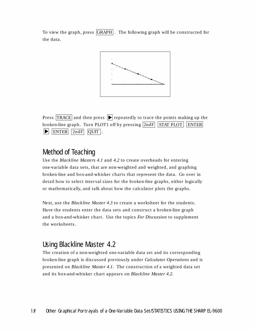
To view the graph, press GRAPH . The following graph will be constructed for
the data.
Press TRACE and then press repeatedly to trace the points making up the
broken-line graph. Turn PLOT1 off by pressing 2ndF STAT PLOT ENTER
ENTER 2ndF QUIT .
Method of TeachingUse the Blackline Masters 4.1 and 4.2 to create overheads for entering
one-variable data sets, that are non-weighted and weighted, and graphing
broken-line and box-and-whisker charts that represent the data. Go over in
detail how to select interval sizes for the broken-line graphs, either logically
or mathematically, and talk about how the calculator plots the graphs.
Next, use the Blackline Master 4.3 to create a worksheet for the students.
Have the students enter the data sets and construct a broken-line graph
and a box-and-whisker chart. Use the topics For Discussion to supplement
the worksheets.
Using Blackline Master 4.2The creation of a non-weighted one-variable data set and its corresponding
broken-line graph is discussed previously under Calculator Operations and is
presented on Blackline Master 4.1. The construction of a weighted data set
and its box-and-whisker chart appears on Blackline Master 4.2.
18 Other Graphical Portrayals of a One-Variable Data Set/STATISTICS USING THE SHARP EL-9600
▼
▼
Press STAT to enter the statistics menu. Delete old data and enter the
following data set in L1 using weights in L2:
1 1 1 2 2 2 2 3 4 4
Move the highlighter to the cell directly below L1. Enter the data by pressing
1 ENTER 2 ENTER 3 ENTER 4 ENTER 3 ENTER 4 ENTER
1 ENTER 2 ENTER .
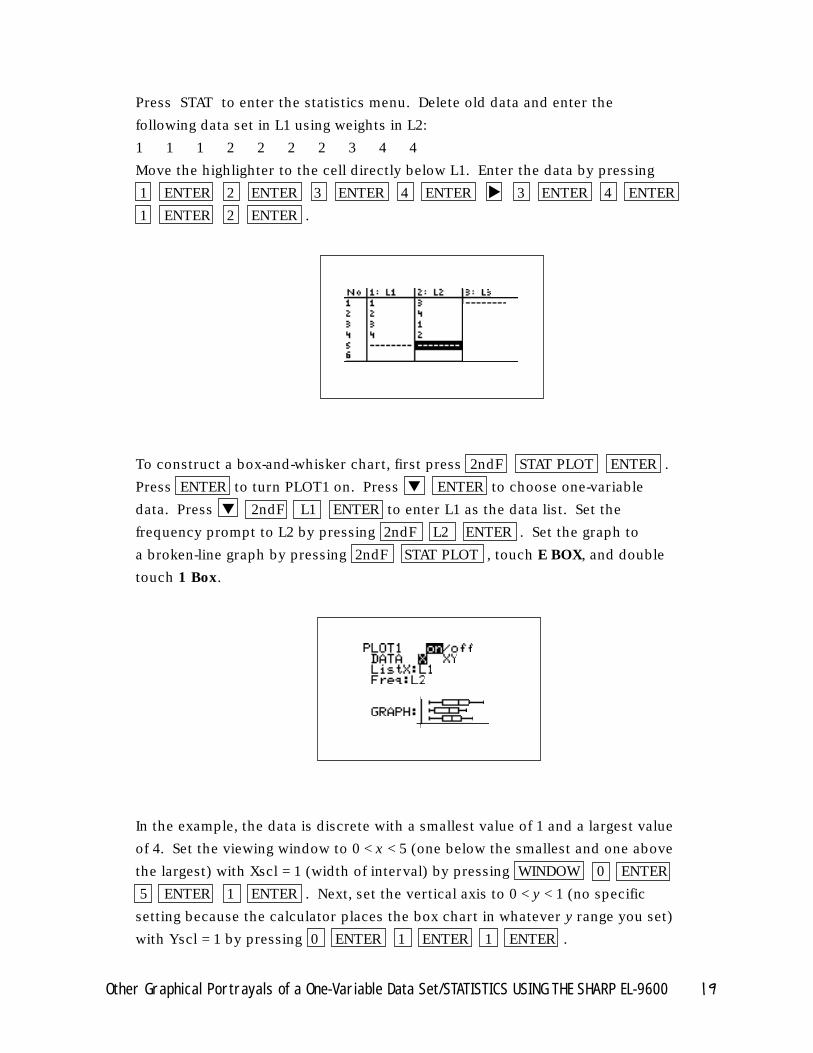
To construct a box-and-whisker chart, first press 2ndF STAT PLOT ENTER .
Press ENTER to turn PLOT1 on. Press ▼ ENTER to choose one-variable
data. Press ▼ 2ndF L1 ENTER to enter L1 as the data list. Set the
frequency prompt to L2 by pressing 2ndF L2 ENTER . Set the graph to
a broken-line graph by pressing 2ndF STAT PLOT , touch E BOX, and double
touch 1 Box.
In the example, the data is discrete with a smallest value of 1 and a largest value
of 4. Set the viewing window to 0 < x < 5 (one below the smallest and one above
the largest) with Xscl = 1 (width of interval) by pressing WINDOW 0 ENTER
5 ENTER 1 ENTER . Next, set the vertical axis to 0 < y < 1 (no specific
setting because the calculator places the box chart in whatever y range you set)
with Yscl = 1 by pressing 0 ENTER 1 ENTER 1 ENTER .
Other Graphical Portrayals of a One-Variable Data Set/STATISTICS USING THE SHARP EL-9600 19
▼
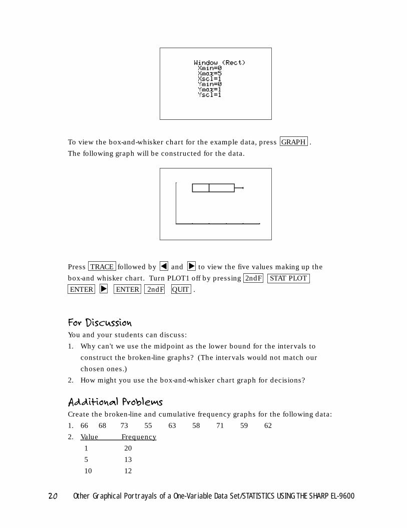
To view the box-and-whisker chart for the example data, press GRAPH .
The following graph will be constructed for the data.
Press TRACE followed by and to view the five values making up the
box-and whisker chart. Turn PLOT1 off by pressing 2ndF STAT PLOT
ENTER ENTER 2ndF QUIT .
For DiscussionYou and your students can discuss:
1. Why can't we use the midpoint as the lower bound for the intervals to
construct the broken-line graphs? (The intervals would not match our
chosen ones.)
2. How might you use the box-and-whisker chart graph for decisions?
Additional ProblemsCreate the broken-line and cumulative frequency graphs for the following data:
1. 66 68 73 55 63 58 71 59 62
2. Value Frequency
1 20
5 13
10 12
20 Other Graphical Portrayals of a One-Variable Data Set/STATISTICS USING THE SHARP EL-9600
▼
▼
▼
Introducing the TopicIn this chapter, you and your students will learn how to create a two-variable
data set.
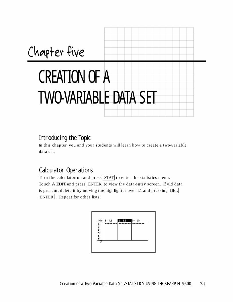
Calculator OperationsTurn the calculator on and press STAT to enter the statistics menu.
Touch A EDIT and press ENTER to view the data-entry screen. If old data
is present, delete it by moving the highlighter over L1 and pressing DEL
ENTER . Repeat for other lists.
Creation of a Two-Variable Data Set/STATISTICS USING THE SHARP EL-9600 21
CREATION OF A TWO-VARIABLE DATA SET
Chapter five
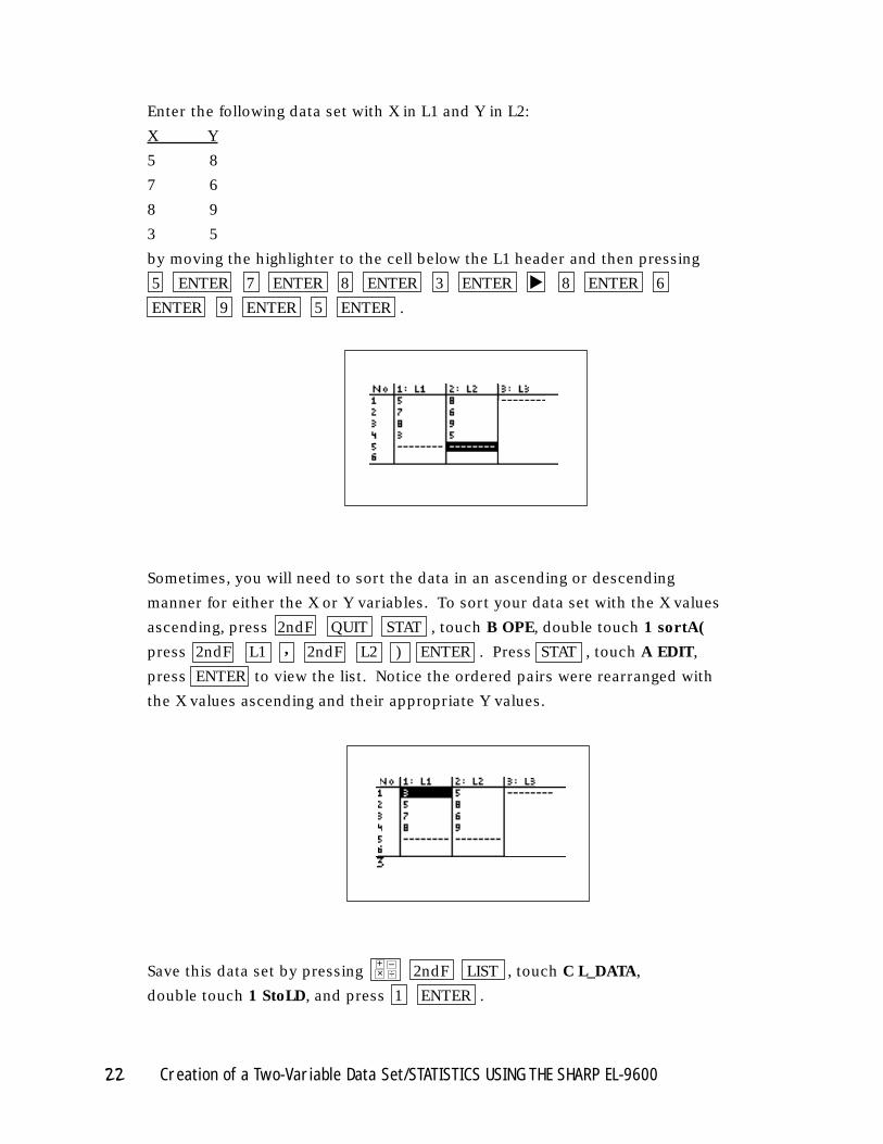
Enter the following data set with X in L1 and Y in L2:
X Y
5 8
7 6
8 9
3 5
by moving the highlighter to the cell below the L1 header and then pressing
5 ENTER 7 ENTER 8 ENTER 3 ENTER 8 ENTER 6
ENTER 9 ENTER 5 ENTER .
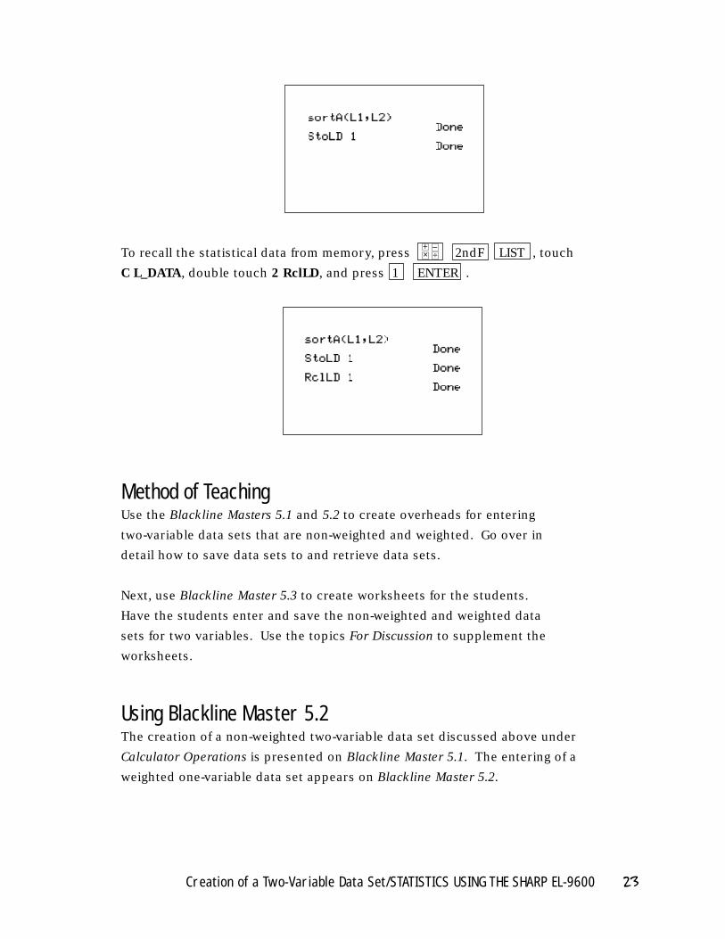
Sometimes, you will need to sort the data in an ascending or descending
manner for either the X or Y variables. To sort your data set with the X values
ascending, press 2ndF QUIT STAT , touch B OPE, double touch 1 sortA(
press 2ndF L1 , 2ndF L2 ) ENTER . Press STAT , touch A EDIT,
press ENTER to view the list. Notice the ordered pairs were rearranged with
the X values ascending and their appropriate Y values.
Save this data set by pressing 2ndF LIST , touch C L_DATA,
double touch 1 StoLD, and press 1 ENTER .
22 Creation of a Two-Variable Data Set/STATISTICS USING THE SHARP EL-9600
▼
×+ –
÷
To recall the statistical data from memory, press 2ndF LIST , touch
C L_DATA, double touch 2 RclLD, and press 1 ENTER .
Method of TeachingUse the Blackline Masters 5.1 and 5.2 to create overheads for entering
two-variable data sets that are non-weighted and weighted. Go over in
detail how to save data sets to and retrieve data sets.
Next, use Blackline Master 5.3 to create worksheets for the students.
Have the students enter and save the non-weighted and weighted data
sets for two variables. Use the topics For Discussion to supplement the
worksheets.
Using Blackline Master 5.2The creation of a non-weighted two-variable data set discussed above under
Calculator Operations is presented on Blackline Master 5.1. The entering of a
weighted one-variable data set appears on Blackline Master 5.2.
Creation of a Two-Variable Data Set/STATISTICS USING THE SHARP EL-9600 23
×+ –
÷
Turn the calculator on and press STAT to enter the statistics menu.
Touch A EDIT and press ENTER to view the data-entry screen. If old data is
present, delete it by moving the highlighter over L1 and pressing DEL ENTER .
Repeat for other lists.
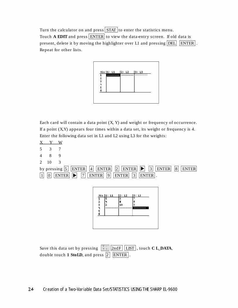
Each card will contain a data point (X, Y) and weight or frequency of occurrence.
If a point (X,Y) appears four times within a data set, its weight or frequency is 4.
Enter the following data set in L1 and L2 using L3 for the weights:
X Y W
5 3 7
4 8 9
2 10 3
by pressing 5 ENTER 4 ENTER 2 ENTER 3 ENTER 8 ENTER
1 0 ENTER 7 ENTER 9 ENTER 3 ENTER .
Save this data set by pressing 2ndF LIST , touch C L_DATA,
double touch 1 StoLD, and press 2 ENTER .
24 Creation of a Two-Variable Data Set/STATISTICS USING THE SHARP EL-9600
▼
▼
×+ –
÷
For DiscussionYou and your students can discuss:
1. What kind of data would come in pairs?
2. What kind of data would possibly come in weighted pairs? (Pairs
occur more than once.)
Creation of a Two-Variable Data Set/STATISTICS USING THE SHARP EL-9600 25
Introducing the TopicIn this chapter, you and your students will learn how to use the Sharp graphing
calculator to find the numerical descriptions of a two-variable data set.
Calculator OperationsTurn the calculator on and press STAT to enter the statistics menu. Touch
A EDIT and press ENTER to access the data entry screen. Delete old data by
highlighting L1 and pressing DEL ENTER . Repeat for other lists.
Enter the following data set:
X Y
25 32
28 33
31 27
40 38
29 30
Please refer to Chapter 5 for discussion on entering a non-weighted two-variable
data set.
26 Numerical Description of a Two-Variable Data Set/STATISTICS USING THE SHARP EL-9600
NUMERICAL DESCRIPTION OF A TWO-VARIABLE DATA SET
Chapter six
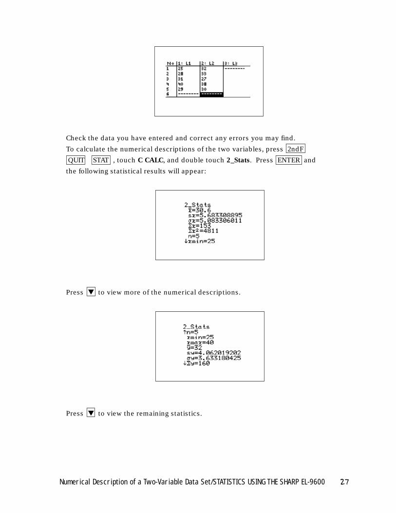
Check the data you have entered and correct any errors you may find.
To calculate the numerical descriptions of the two variables, press 2ndF
QUIT STAT , touch C CALC, and double touch 2_Stats. Press ENTER and
the following statistical results will appear:
Press ▼ to view more of the numerical descriptions.
Press ▼ to view the remaining statistics.
Numerical Description of a Two-Variable Data Set/STATISTICS USING THE SHARP EL-9600 27
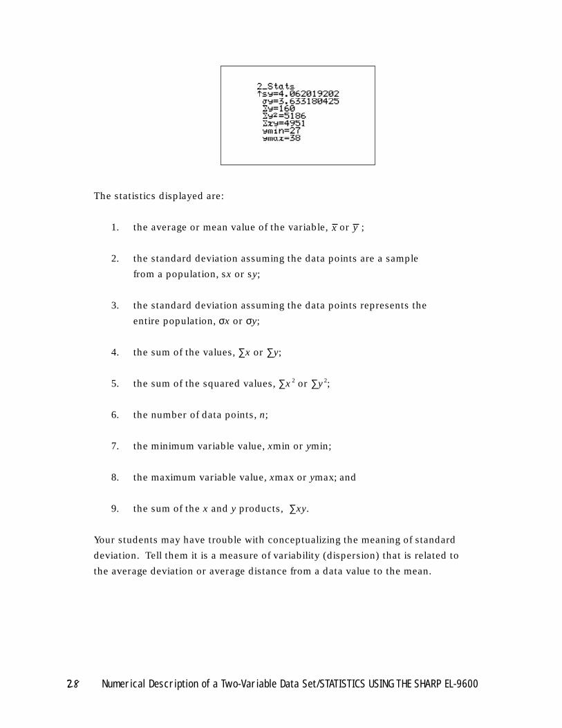
The statistics displayed are:
1. the average or mean value of the variable, or ;
2. the standard deviation assuming the data points are a sample
from a population, sx or sy;
3. the standard deviation assuming the data points represents the
entire population, σx or σy;
4. the sum of the values, ∑x or ∑y;
5. the sum of the squared values, ∑x 2 or ∑y 2;
6. the number of data points, n;
7. the minimum variable value, xmin or ymin;
8. the maximum variable value, xmax or ymax; and
9. the sum of the x and y products, ∑xy.
Your students may have trouble with conceptualizing the meaning of standard
deviation. Tell them it is a measure of variability (dispersion) that is related to
the average deviation or average distance from a data value to the mean.
28 Numerical Description of a Two-Variable Data Set/STATISTICS USING THE SHARP EL-9600
x y
Method of TeachingUse Blackline Master 6.1 to create an overhead for calculating the numerical
descriptions of a two-variable data set. Go over in detail the statistics provided
by the calculator.
Next, use Blackline Masters 6.2 and 6.3 to create work sheets for the students.
Have the students enter and save the non-weighted and weighted two-variable
data sets, and then compute the numerical descriptions. Use the topics For
Discussion to supplement the worksheets.
Using Blackline Master 6.2Turn the calculator on and press STAT to enter the statistics menu. Delete old
data set by highlighting L1 and pressing DEL ENTER . Repeat for other lists.
Enter the following data set which represents the frequency of observing
doubles with a particular pair of dice. The dice were rolled until fifty doubles
were observed.
X Y W
1 1 8
2 2 10
3 3 12
4 4 9
5 5 6
6 6 5
Each row will contain a data pair and the frequency of occurrence.
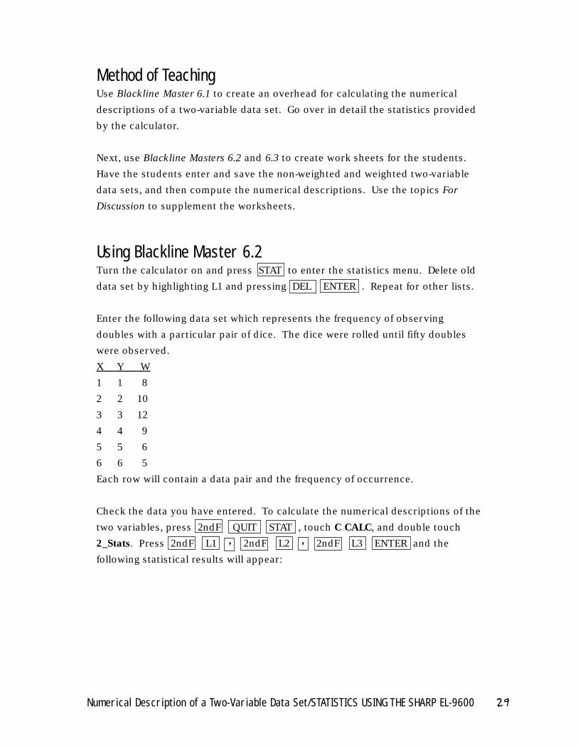
Check the data you have entered. To calculate the numerical descriptions of the
two variables, press 2ndF QUIT STAT , touch C CALC, and double touch
2_Stats. Press 2ndF L1 , 2ndF L2 , 2ndF L3 ENTER and the
following statistical results will appear:
Numerical Description of a Two-Variable Data Set/STATISTICS USING THE SHARP EL-9600 29
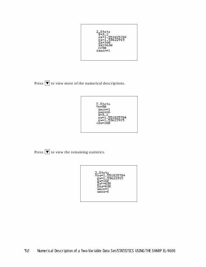
Press ▼ to view more of the numerical descriptions.
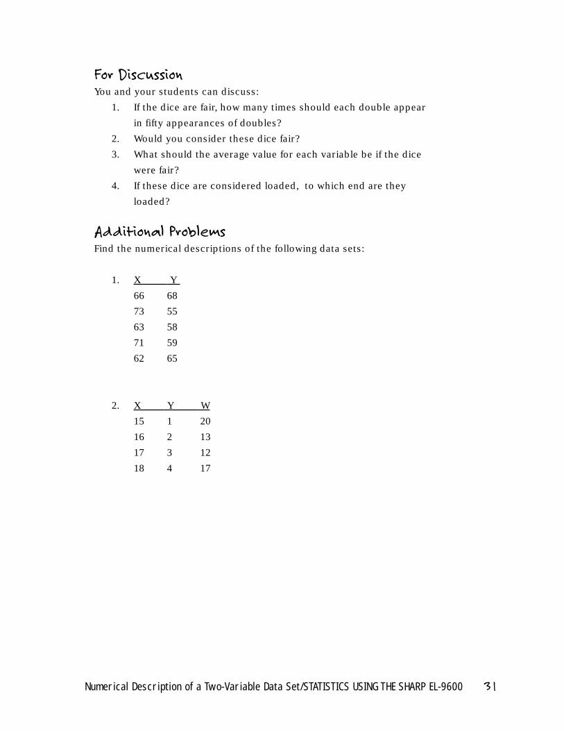
Press ▼ to view the remaining statistics.
30 Numerical Description of a Two-Variable Data Set/STATISTICS USING THE SHARP EL-9600
For DiscussionYou and your students can discuss:
1. If the dice are fair, how many times should each double appear
in fifty appearances of doubles?
2. Would you consider these dice fair?
3. What should the average value for each variable be if the dice
were fair?
4. If these dice are considered loaded, to which end are they
loaded?
Additional ProblemsFind the numerical descriptions of the following data sets:
1. X Y
66 68
73 55
63 58
71 59
62 65
2. X Y W
15 1 20
16 2 13
17 3 12
18 4 17
Numerical Description of a Two-Variable Data Set/STATISTICS USING THE SHARP EL-9600 31
Introducing the TopicIn this chapter, you and your students will learn how to use the Sharp graphing
calculator to graphically portray a two-variable data set with a statistical graph
called a scatter diagram or scatter plot.
Calculator OperationsBefore drawing a scatter diagram, data must be entered on the statistics data
entry screen. You can either enter new data or recall a data set that has been
stored within a matrix. (Refer to Chapter 5 for discussion on entering, storing
and/or recalling a two-variable data set.) Consider the following table listing the
revenue for a large corporation:
Year Revenue (in millions of dollars)
1990 48.63
1991 48.86
1992 48.91
1993 49.69
1994 51.10
1995 52.00
1996 52.03
32 Graphical Portrayal of a Two-Variable Data Set/STATISTICS USING THE SHARP EL-9600
GRAPHICAL PORTRAYAL OF A TWO-VARIABLE DATA SET
Chapter seven
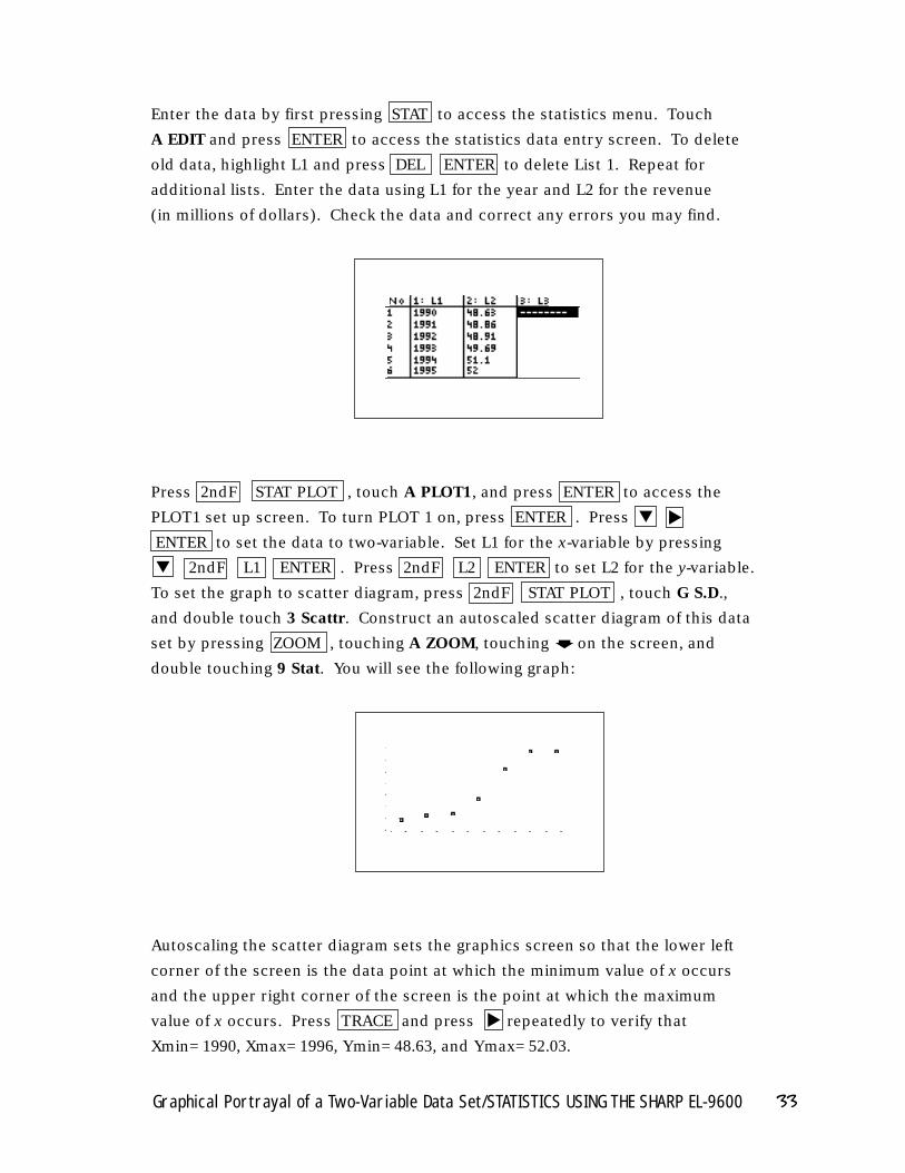
Enter the data by first pressing STAT to access the statistics menu. Touch
A EDIT and press ENTER to access the statistics data entry screen. To delete
old data, highlight L1 and press DEL ENTER to delete List 1. Repeat for
additional lists. Enter the data using L1 for the year and L2 for the revenue
(in millions of dollars). Check the data and correct any errors you may find.
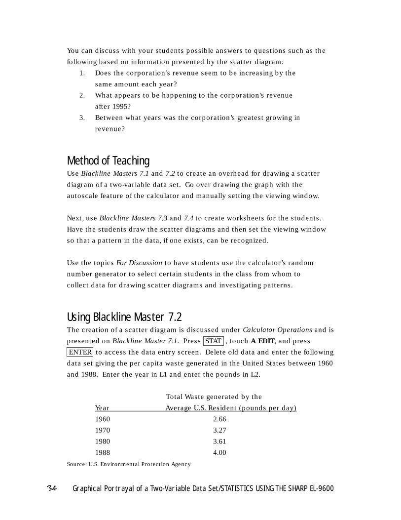
Press 2ndF STAT PLOT , touch A PLOT1, and press ENTER to access the
PLOT1 set up screen. To turn PLOT 1 on, press ENTER . Press ▼
ENTER to set the data to two-variable. Set L1 for the x-variable by pressing
▼ 2ndF L1 ENTER . Press 2ndF L2 ENTER to set L2 for the y-variable.
To set the graph to scatter diagram, press 2ndF STAT PLOT , touch G S.D.,
and double touch 3 Scattr. Construct an autoscaled scatter diagram of this data
set by pressing ZOOM , touching A ZOOM, touching on the screen, and
double touching 9 Stat. You will see the following graph:
Autoscaling the scatter diagram sets the graphics screen so that the lower left
corner of the screen is the data point at which the minimum value of x occurs
and the upper right corner of the screen is the point at which the maximum
value of x occurs. Press TRACE and press repeatedly to verify that
Xmin= 1990, Xmax= 1996, Ymin= 48.63, and Ymax= 52.03.
Graphical Portrayal of a Two-Variable Data Set/STATISTICS USING THE SHARP EL-9600 33
▼
▼
➧
You can discuss with your students possible answers to questions such as the
following based on information presented by the scatter diagram:
1. Does the corporation’s revenue seem to be increasing by the
same amount each year?
2. What appears to be happening to the corporation’s revenue
after 1995?
3. Between what years was the corporation’s greatest growing in
revenue?
Method of TeachingUse Blackline Masters 7.1 and 7.2 to create an overhead for drawing a scatter
diagram of a two-variable data set. Go over drawing the graph with the
autoscale feature of the calculator and manually setting the viewing window.
Next, use Blackline Masters 7.3 and 7.4 to create worksheets for the students.
Have the students draw the scatter diagrams and then set the viewing window
so that a pattern in the data, if one exists, can be recognized.
Use the topics For Discussion to have students use the calculator’s random
number generator to select certain students in the class from whom to
collect data for drawing scatter diagrams and investigating patterns.
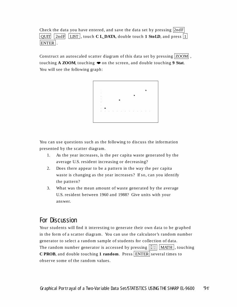
Using Blackline Master 7.2The creation of a scatter diagram is discussed under Calculator Operations and is
presented on Blackline Master 7.1. Press STAT , touch A EDIT, and press
ENTER to access the data entry screen. Delete old data and enter the following
data set giving the per capita waste generated in the United States between 1960
and 1988. Enter the year in L1 and enter the pounds in L2.
Total Waste generated by the
Year Average U.S. Resident (pounds per day)
1960 2.66
1970 3.27
1980 3.61
1988 4.00
Source: U.S. Environmental Protection Agency
34 Graphical Portrayal of a Two-Variable Data Set/STATISTICS USING THE SHARP EL-9600
Check the data you have entered, and save the data set by pressing 2ndF
QUIT 2ndF LIST , touch C L_DATA, double touch 1 StoLD, and press 1
ENTER .
Construct an autoscaled scatter diagram of this data set by pressing ZOOM ,
touching A ZOOM, touching on the screen, and double touching 9 Stat.
You will see the following graph:
You can use questions such as the following to discuss the information
presented by the scatter diagram.
1. As the year increases, is the per capita waste generated by the
average U.S. resident increasing or decreasing?
2. Does there appear to be a pattern in the way the per capita
waste is changing as the year increases? If so, can you identify
the pattern?
3. What was the mean amount of waste generated by the average
U.S. resident between 1960 and 1988? Give units with your
answer.
For DiscussionYour students will find it interesting to generate their own data to be graphed
in the form of a scatter diagram. You can use the calculator’s random number
generator to select a random sample of students for collection of data.
The random number generator is accessed by pressing MATH , touching
C PROB, and double touching 1 random. Press ENTER several times to
observe some of the random values.
Graphical Portrayal of a Two-Variable Data Set/STATISTICS USING THE SHARP EL-9600 35
➧
×+ –
÷
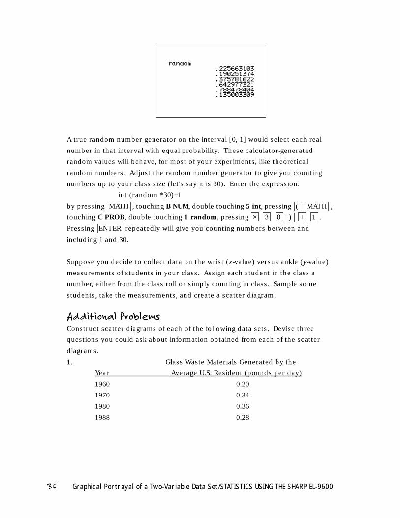
A true random number generator on the interval [0, 1] would select each real
number in that interval with equal probability. These calculator-generated
random values will behave, for most of your experiments, like theoretical
random numbers. Adjust the random number generator to give you counting
numbers up to your class size (let's say it is 30). Enter the expression:
int (random *30)+1
by pressing MATH , touching B NUM, double touching 5 int, pressing ( MATH ,
touching C PROB, double touching 1 random, pressing × 3 0 ) + 1 .
Pressing ENTER repeatedly will give you counting numbers between and
including 1 and 30.
Suppose you decide to collect data on the wrist (x-value) versus ankle (y-value)
measurements of students in your class. Assign each student in the class a
number, either from the class roll or simply counting in class. Sample some
students, take the measurements, and create a scatter diagram.
Additional ProblemsConstruct scatter diagrams of each of the following data sets. Devise three
questions you could ask about information obtained from each of the scatter
diagrams.
1. Glass Waste Materials Generated by the
Year Average U.S. Resident (pounds per day)
1960 0.20
1970 0.34
1980 0.36
1988 0.28
36 Graphical Portrayal of a Two-Variable Data Set/STATISTICS USING THE SHARP EL-9600
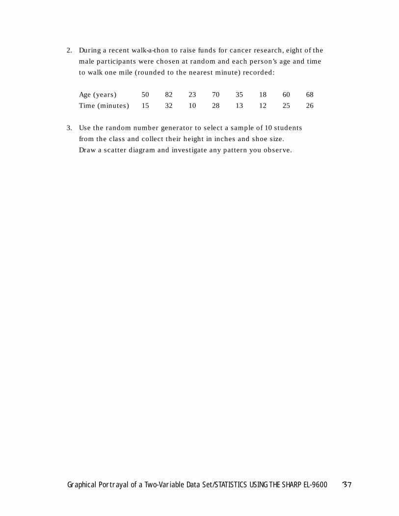
2. During a recent walk-a-thon to raise funds for cancer research, eight of the
male participants were chosen at random and each person’s age and time
to walk one mile (rounded to the nearest minute) recorded:
Age (years) 50 82 23 70 35 18 60 68
Time (minutes) 15 32 10 28 13 12 25 26
3. Use the random number generator to select a sample of 10 students
from the class and collect their height in inches and shoe size.
Draw a scatter diagram and investigate any pattern you observe.
Graphical Portrayal of a Two-Variable Data Set/STATISTICS USING THE SHARP EL-9600 37
Introducing the TopicIn this chapter, you and your students will learn how to use the Sharp graphing
calculator to find the linear regression (best-fitting line) for a set of data points.
A regression line is a linear model of the relationship between the dependent
variable Y and the independent variable X. The model is denoted as Y = a + bX,
where a is the Y-intercept and b is the slope of the regression line.
A third value, r, is calculated for each regression. The r value is the correlation
coefficient, which is a measure of how well the line fits the data points, and it
will range from -1 to 1. If r = -1 or 1, then the line intersects all the data points,
and the data points are said to be in perfect-linear correlation. A positive sign
indicates a direct relationship (as X increases, the Y increases), whereas a
negative sign indicates an indirect relationship (as X increases, the Y decreases).
Values of r close to -1 or 1 are said to reflect a strong linear correlation, and
values close to 0 are said to reflect the absence of linear correlation.
38 Linear Regressions/STATISTICS USING THE SHARP EL-9600
LINEAR REGRESSIONSChapter eight
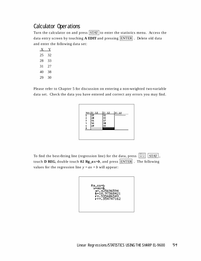
Calculator OperationsTurn the calculator on and press STAT to enter the statistics menu. Access the
data entry screen by touching A EDIT and pressing ENTER . Delete old data
and enter the following data set:
X Y
25 32
28 33
31 27
40 38
29 30
Please refer to Chapter 5 for discussion on entering a non-weighted two-variable
data set. Check the data you have entered and correct any errors you may find.
To find the best-fitting line (regression line) for the data, press STAT ,
touch D REG, double touch 02 Rg_ax+b, and press ENTER . The following
values for the regression line y = ax + b will appear:
Linear Regressions/STATISTICS USING THE SHARP EL-9600 39
×+ –
÷
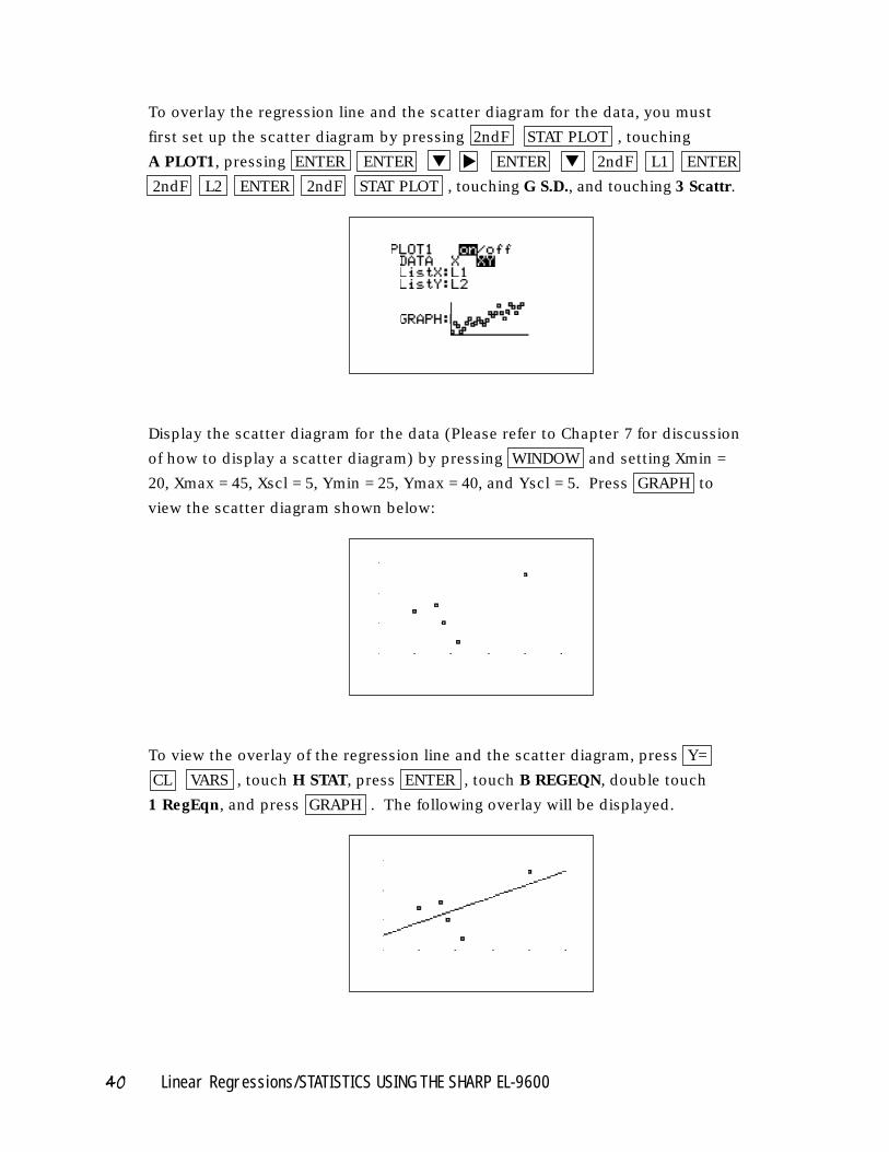
To overlay the regression line and the scatter diagram for the data, you must
first set up the scatter diagram by pressing 2ndF STAT PLOT , touching
A PLOT1, pressing ENTER ENTER ▼ ENTER ▼ 2ndF L1 ENTER
2ndF L2 ENTER 2ndF STAT PLOT , touching G S.D., and touching 3 Scattr.
Display the scatter diagram for the data (Please refer to Chapter 7 for discussion
of how to display a scatter diagram) by pressing WINDOW and setting Xmin =
20, Xmax = 45, Xscl = 5, Ymin = 25, Ymax = 40, and Yscl = 5. Press GRAPH to
view the scatter diagram shown below:
To view the overlay of the regression line and the scatter diagram, press Y=
CL VARS , touch H STAT, press ENTER , touch B REGEQN, double touch
1 RegEqn, and press GRAPH . The following overlay will be displayed.
40 Linear Regressions/STATISTICS USING THE SHARP EL-9600
▼
Method of TeachingUse Blackline Masters 8.1 and 8.2 to create overheads for demonstrating the
calculation of a regression line for a set of data points, and the display of an
overlay of the scatter diagram for the data points and the regression line. Go over
in detail the significance of the a, b, and r values generated by the calculator.
Next, use Blackline Master 8.3 to create a worksheet for the students. Have
the students enter the data points, compute the regression line, and display
the overlay of the scatter diagram and regression line. Use the topics For
Discussion to supplement the worksheets.
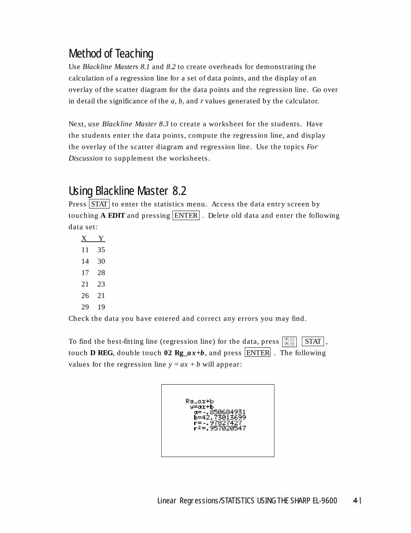
Using Blackline Master 8.2Press STAT to enter the statistics menu. Access the data entry screen by
touching A EDIT and pressing ENTER . Delete old data and enter the following
data set:
X Y
11 35
14 30
17 28
21 23
26 21
29 19
Check the data you have entered and correct any errors you may find.
To find the best-fitting line (regression line) for the data, press STAT ,
touch D REG, double touch 02 Rg_ax+b, and press ENTER . The following
values for the regression line y = ax + b will appear:
Linear Regressions/STATISTICS USING THE SHARP EL-9600 41
×+ –
÷
To overlay the regression line and the scatter diagram for the data, you must
first set up the scatter diagram by pressing 2ndF STAT PLOT , touching
A PLOT1, pressing ENTER ENTER ▼ ENTER ▼ 2ndF L1 ENTER
2ndF L2 ENTER 2ndF STAT PLOT , touching G S.D., and double touching
3 Scattr.
Display the scatter diagram for the data by pressing WINDOW and setting
Xmin = 10, Xmax = 30, Xscl = 5, Ymin = 15, Ymax = 40, and Yscl = 5. Press Y=
CL to clear any previously entered expressions. Press GRAPH to view the
scatter diagram.
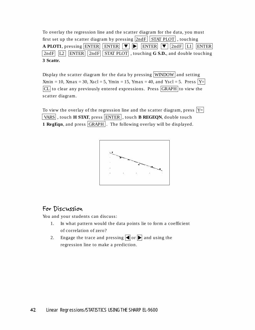
To view the overlay of the regression line and the scatter diagram, press Y=
VARS , touch H STAT, press ENTER , touch B REGEQN, double touch
1 RegEqn, and press GRAPH . The following overlay will be displayed.
For DiscussionYou and your students can discuss:
1. In what pattern would the data points lie to form a coefficient
of correlation of zero?
2. Engage the trace and pressing or and using the
regression line to make a prediction.
42 Linear Regressions/STATISTICS USING THE SHARP EL-9600
▼▼
▼
Additional ProblemsFind the equation for the regression lines, and construct the overlays of the
scatter diagram and regression lines for the following data sets:
X Y
1. 66 68 60 < X < 75, scale of 1
73 55 50 < Y < 70, scale of 5
63 58
71 59
62 65
2. X Y
1500 99 1400 < X < 1900, scale of 100
1600 201 0 < Y < 500, scale of 100
1700 295
1800 403
Linear Regressions/STATISTICS USING THE SHARP EL-9600 43
Introducing the TopicIn this chapter, you and your students will learn how to use the Sharp graphing
calculator to find several regression equations for a set of data points and then
determine the model of "best fit." A regression equation is a model of the
relationship between the dependent variable Y and the independent variable X.
Other regression models include y = ax 2 + bx + c (quadratic), y = ax 3 + bx 2 + cx +
d (cubic), y = ax4 + bx 3 + cx 2 + dx + e (quartic), y = a + b ln x (natural logarithm),
y = a + b log x (common logarithm), y = a*bx (exponential), y = a*ebX (natural
exponential), y = a + bx-1 (inverse), and Y = a*Xb (power). The a, b, c, d and e are
calculated for each model in order to find the best-fitting curve (minimized error).
A third value, r 2, is calculated for each regression and is a measure of how well
the equation fits the data points, and it will range from 0 to 1. If r 2 = 1, then the
equation intersects all the data points, and the model is said to have perfect fit.
Values of r 2 close to 1 are said to reflect a good fit, and values close to 0 are said
to reflect a poor fit.
44 Other Regressions and Model of “Best Fit”/STATISTICS USING THE SHARP EL-9600
OTHER REGRESSIONS AND MODEL OF “BEST FIT”
Chapter nine
Calculator OperationsTurn the calculator on and press STAT to enter the statistics menu. Touch
A EDIT and press ENTER to access the data entry screen. Delete old data
and enter the following data set:
X Y
6 10
22 19
34 31
42 39
45 47
48 58
47 66
Please refer to Chapter 5 for discussion on entering a non-weighted two-variable
data set. Check the data you have entered and correct any errors you may find.
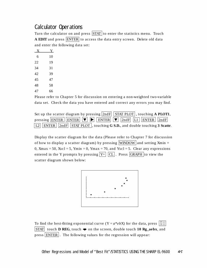
Set up the scatter diagram by pressing 2ndF STAT PLOT , touching A PLOT1,
pressing ENTER ENTER ▼ ENTER ▼ 2ndF L1 ENTER 2ndF
L2 ENTER 2ndF STAT PLOT , touching G S.D., and double touching 3 Scattr.
Display the scatter diagram for the data (Please refer to Chapter 7 for discussion
of how to display a scatter diagram) by pressing WINDOW and setting Xmin =
0, Xmax = 50, Xscl = 5, Ymin = 0, Ymax = 70, and Yscl = 5. Clear any expressions
entered in the Y prompts by pressing Y= CL . Press GRAPH to view the
scatter diagram shown below:
To find the best-fitting exponential curve (Y = a*ebX) for the data, press
STAT touch D REG, touch on the screen, double touch 10 Rg_aebx, and
press ENTER . The following values for the regression will appear:
▼
×+ –
÷
➧
Other Regressions and Model of “Best Fit”/STATISTICS USING THE SHARP EL-9600 45
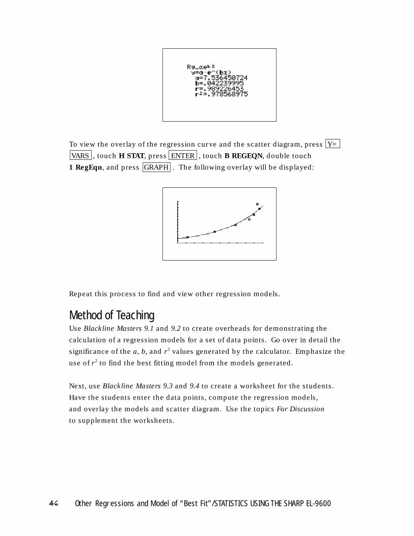
To view the overlay of the regression curve and the scatter diagram, press Y=
VARS , touch H STAT, press ENTER , touch B REGEQN, double touch
1 RegEqn, and press GRAPH . The following overlay will be displayed:
Repeat this process to find and view other regression models.
Method of TeachingUse Blackline Masters 9.1 and 9.2 to create overheads for demonstrating the
calculation of a regression models for a set of data points. Go over in detail the
significance of the a, b, and r 2 values generated by the calculator. Emphasize the
use of r 2 to find the best fitting model from the models generated.
Next, use Blackline Masters 9.3 and 9.4 to create a worksheet for the students.
Have the students enter the data points, compute the regression models,
and overlay the models and scatter diagram. Use the topics For Discussion
to supplement the worksheets.
46 Other Regressions and Model of “Best Fit”/STATISTICS USING THE SHARP EL-9600
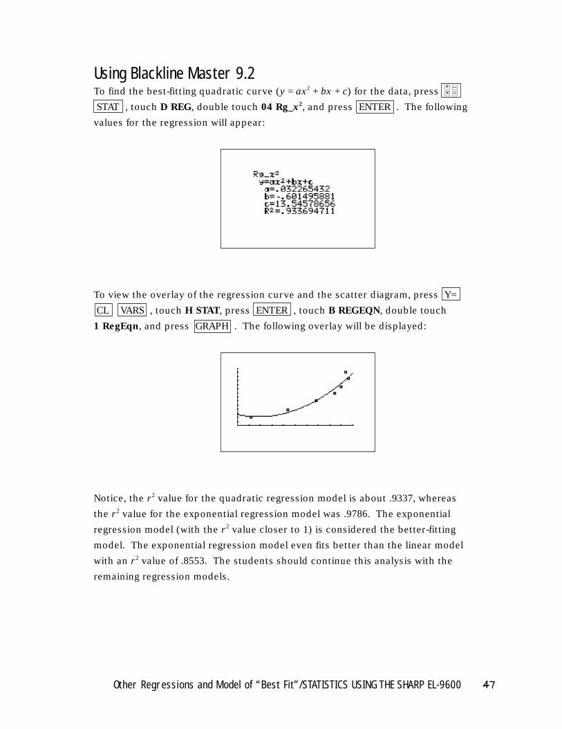
Using Blackline Master 9.2To find the best-fitting quadratic curve (y = ax2 + bx + c) for the data, press
STAT , touch D REG, double touch 04 Rg_x2, and press ENTER . The following
values for the regression will appear:
To view the overlay of the regression curve and the scatter diagram, press Y=
CL VARS , touch H STAT, press ENTER , touch B REGEQN, double touch
1 RegEqn, and press GRAPH . The following overlay will be displayed:
Notice, the r 2 value for the quadratic regression model is about .9337, whereas
the r 2 value for the exponential regression model was .9786. The exponential
regression model (with the r 2 value closer to 1) is considered the better-fitting
model. The exponential regression model even fits better than the linear model
with an r 2 value of .8553. The students should continue this analysis with the
remaining regression models.
Other Regressions and Model of “Best Fit”/STATISTICS USING THE SHARP EL-9600 47
×+ –
÷
For DiscussionYou and your students can discuss:
1. Can you tell from the graphs which model fits the best?
2. Engage the trace and press or to move the tracer along the
curve, or from data point to data point. Press ▲ or ▼ to move from
the curve to the data points, or vice versa. Use this mechanism to find
the error between a predicted Y value (on the regression curve) and a
known Y value for a given X (one of the known points).
Additional ProblemFind the best-fitting regression model for the following data set:
X Y
66 68 60 < X < 75, scale of 1
73 55 50 < Y < 70, scale of 5
63 58
71 59
62 65
69 61
74 60
65 60
63 60
79 49
48 Other Regressions and Model of “Best Fit”/STATISTICS USING THE SHARP EL-9600
▼▼
Introducing the TopicIn this chapter, you and your students will learn how to use the Sharp graphing
calculator to perform several statistical tests. A statistical test assists in making
a decision between two hypotheses. A statistical test contains five components:
a null hypothesis, an alternate hypothesis, an observed statistic from the
sample, a rejection statistic for making a decision, and the decision itself.
The null hypothesis is generally a statement of equality, whereas the alternate
hypothesis is a statement of inequality (≠, <, or >). Each of the five components
of the statistical test will be identified in each problem addressed.
Calculator OperationsTurn the calculator on and press STAT to enter the statistics menu.
Touch A EDIT and press ENTER to access the data entry screen.
Delete old data and enter the following data set for L1:
7 10 7 6 8 10 15 14 11
12 6 11 11 5 7 9 9 7
Check the data you have entered and correct any errors you may find.
Statistical Tests/STATISTICS USING THE SHARP EL-9600 49
STATISTICAL TESTSChapter ten
The data shown above reflects the number of wins for the Chicago Bears in each
season since 1978 when the NFL went to a 16 game season. The only season left
out was the 1982 strike shortened season. Test the alternate hypothesis that
"da Bears" are a winning football team against the null hypothesis that "da
Bears" are merely a .500 ball club.
Set up the statistical test by pressing 2ndF QUIT STAT , touching E TEST,
and double touching 03 Ttest1samp. The one-sample T test was chosen
because we have one small sample and we do not know the standard deviation.
If we had a sample larger than 30 or knew the standard deviation, then we could
use the Ztest1samp command. If we had two small samples or did not know the
standard deviations, then we would use Ttest2samp. If we had two large
samples or knew the standard deviations, then we could use the Ztest2samp.
All of these tests are for testing equality of a mean to a number (one sample
test) or equality of two means (two sample).
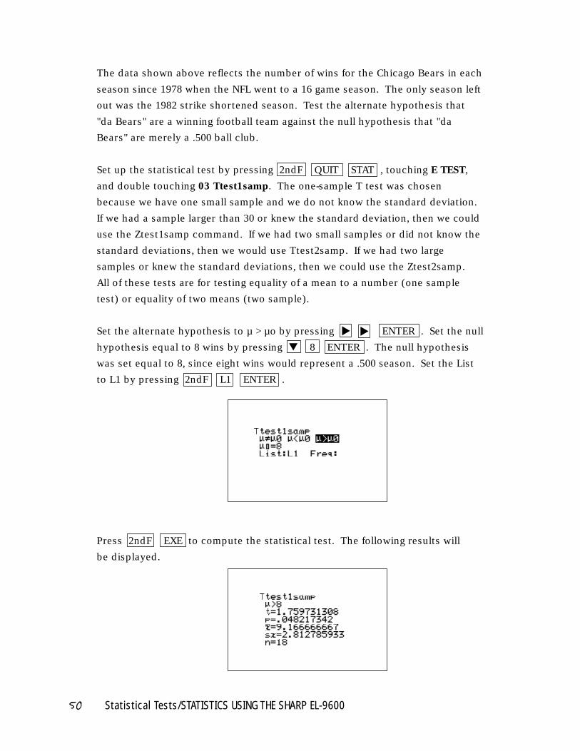
Set the alternate hypothesis to µ > µo by pressing ENTER . Set the null
hypothesis equal to 8 wins by pressing ▼ 8 ENTER . The null hypothesis
was set equal to 8, since eight wins would represent a .500 season. Set the List
to L1 by pressing 2ndF L1 ENTER .
Press 2ndF EXE to compute the statistical test. The following results will
be displayed.
50 Statistical Tests/STATISTICS USING THE SHARP EL-9600
▼ ▼
The first item on the screen, µ>8, is the alternate hypothesis of the statistical
test. Supporting the alternate hypothesis in this case would mean "da Bears," on
the average, win more than 8 games in a season and thus are a winning ball team.
The null hypothesis is not shown on the screen because it is always the same as
the alternate except it is an equality (µ=8). The second item on the screen is the
observed statistic from the sample (observed t ). From it, the third item on
the screen is calculated and it represents the decision statistic (p value).
Typically in science, the .05 level of significance is used in making decisions.
Deviation from this level of significance would need to be defended in a report.
A .05 level of significance means that if our observed statistic from the sample
falls in the rare 5%, we will reject the null hypothesis and support the alternate
hypothesis.
Therefore, if your p value is less than .05 you will reject the null hypothesis and
support the alternate hypothesis. In our problem, the p value is .0482 which
is less than .05. Our decision is to reject the null hypothesis that µ=8 and
support the alternate hypothesis that µ>8. This test clearly shows that "da
Bears" average more than 8 wins a season and thus are a winning football team.
If the p value is greater than .05 you would support the null hypothesis that µ=8.
The fourth, fifth and sixth items on the screen show the sample average,
sample standard deviation and sample size. On the average, "da Bears"
win approximately 9 games a season.
Method of TeachingUse Blackline Masters 10.1 and 10.2 to create overheads for performing statistical
tests. Go over in detail the five parts of a statistical test and the items generated
by the calculator.
Next, use Blackline Master 10.3 to create a worksheet for the students. Have the
students enter the data points, compute the regression models, and overlay the
models and scatter diagram. Use the topics For Discussion to supplement the
worksheets.
Statistical Tests/STATISTICS USING THE SHARP EL-9600 51
Using Blackline Master 10.2Press STAT to enter the statistics menu. Touch A EDIT and press ENTER to
access the data entry screen. Enter the additional data for L2:
L1 Bears 7 10 7 6 8 10 15 14 11
12 6 11 11 5 7 9 9 7
L2 Packers 8 5 5 8 8 8 8 4 5
4 10 6 4 9 9 9 11 13
Check the data you have entered and correct any errors you may find.
The data shown above reflects the number of wins for the Chicago Bears and
Green Bay Packers in each season since 1978 when the NFL went to a 16 game
season. The only season left out was the 1982 strike shortened season. Test
the alternate hypothesis that "da Bears" are a better (on the average won more
games) football team than the Packers during these recent years. Each won one
Super Bowl during this time. The null hypothesis would be that "da Bears" are
merely equal to the Packers.
Set up the statistical test by pressing 2ndF QUIT STAT , touching E TEST,
and double touching 04 Ttest2samp. The two-sample T test was chosen
because we have two small samples.
Set the alternate hypothesis to µ1 > µ2 by pressing ENTER . Pool the
standard deviations in the calculation by pressing ▼ ENTER . We pool
the standard deviations for the statistical test when the standard deviations are
approximately equal. Statistical analysis of each data set showed they were
nearly the same. Do not pool the standard deviations when they are subjectively
unequal. Set the List1 to L1 by pressing ▼ 2ndF L1 ENTER . Set List2 to
L2 by pressing 2ndF L2 ENTER .
52 Statistical Tests/STATISTICS USING THE SHARP EL-9600
▼ ▼▼
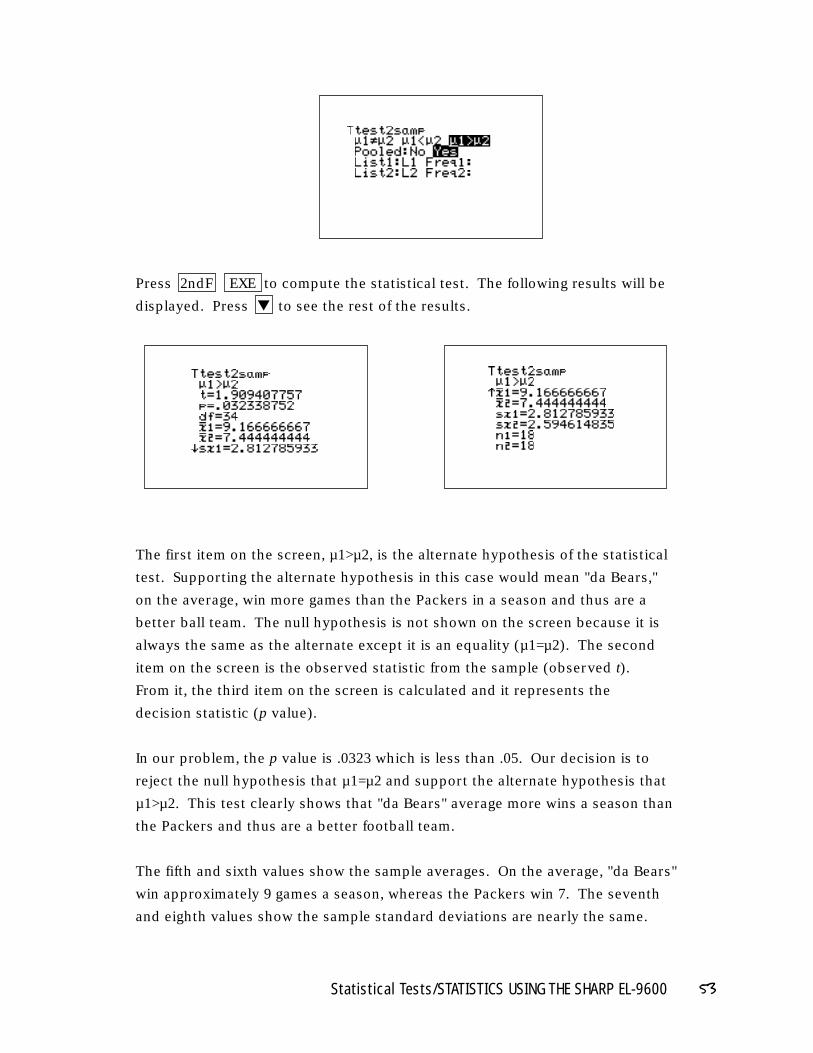
Press 2ndF EXE to compute the statistical test. The following results will be
displayed. Press ▼ to see the rest of the results.
The first item on the screen, µ1>µ2, is the alternate hypothesis of the statistical
test. Supporting the alternate hypothesis in this case would mean "da Bears,"
on the average, win more games than the Packers in a season and thus are a
better ball team. The null hypothesis is not shown on the screen because it is
always the same as the alternate except it is an equality (µ1=µ2). The second
item on the screen is the observed statistic from the sample (observed t).
From it, the third item on the screen is calculated and it represents the
decision statistic (p value).
In our problem, the p value is .0323 which is less than .05. Our decision is to
reject the null hypothesis that µ1=µ2 and support the alternate hypothesis that
µ1>µ2. This test clearly shows that "da Bears" average more wins a season than
the Packers and thus are a better football team.
The fifth and sixth values show the sample averages. On the average, "da Bears"
win approximately 9 games a season, whereas the Packers win 7. The seventh
and eighth values show the sample standard deviations are nearly the same.
Statistical Tests/STATISTICS USING THE SHARP EL-9600 53
For DiscussionYou and your students can discuss:
1. using the Ztest1samp and Ztest2samp for large samples (n>30)
or when the standard deviation(s) is/are known.
2. using the Ftest2samp for testing the standard deviations for
two samples.
Additional Problem1. The length of stay in days for 20 randomly selected hospital patients
are provided below. Enter the data in L1 and test the alternate
hypothesis that the average length of stay is less than 5 days.
2 3 8 6 4 4 6 4 2 5
3 5 2 3 3 2 10 2 4 2
2. The reading scores for two separate classes are provided below.
Enter Class 1's scores into L1 and Class 2's scores into L2. Test
the alternative hypothesis that Class 1 reads better than Class 2.
Pool the standard deviations for the test.
Class 1 87 84 92 83 97 79 76 90
Class 2 82 78 86 78 94 78 71 86
54 Statistical Tests/STATISTICS USING THE SHARP EL-9600
Blackline Masters/STATISTICS USING THE SHARP EL-9600 55
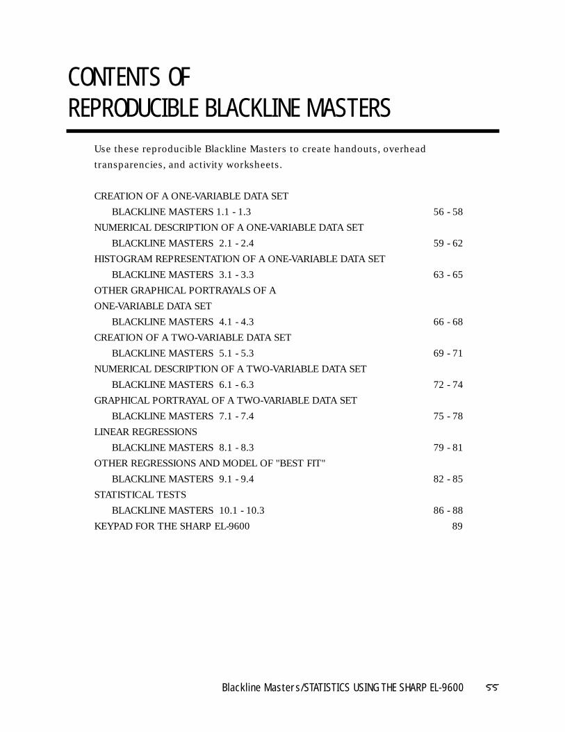
CONTENTS OF REPRODUCIBLE BLACKLINE MASTERS
Use these reproducible Blackline Masters to create handouts, overhead
transparencies, and activity worksheets.
CREATION OF A ONE-VARIABLE DATA SET
BLACKLINE MASTERS 1.1 - 1.3 56 - 58
NUMERICAL DESCRIPTION OF A ONE-VARIABLE DATA SET
BLACKLINE MASTERS 2.1 - 2.4 59 - 62
HISTOGRAM REPRESENTATION OF A ONE-VARIABLE DATA SET
BLACKLINE MASTERS 3.1 - 3.3 63 - 65
OTHER GRAPHICAL PORTRAYALS OF A
ONE-VARIABLE DATA SET
BLACKLINE MASTERS 4.1 - 4.3 66 - 68
CREATION OF A TWO-VARIABLE DATA SET
BLACKLINE MASTERS 5.1 - 5.3 69 - 71
NUMERICAL DESCRIPTION OF A TWO-VARIABLE DATA SET
BLACKLINE MASTERS 6.1 - 6.3 72 - 74
GRAPHICAL PORTRAYAL OF A TWO-VARIABLE DATA SET
BLACKLINE MASTERS 7.1 - 7.4 75 - 78
LINEAR REGRESSIONS
BLACKLINE MASTERS 8.1 - 8.3 79 - 81
OTHER REGRESSIONS AND MODEL OF "BEST FIT"
BLACKLINE MASTERS 9.1 - 9.4 82 - 85
STATISTICAL TESTS
BLACKLINE MASTERS 10.1 - 10.3 86 - 88
KEYPAD FOR THE SHARP EL-9600 89
56 Blackline Masters/STATISTICS USING THE SHARP EL-9600Cop
yrig
ht ©
1998
, S
harp
Ele
ctro
nics
Cor
pora
tion.
Per
mis
sion
is g
rant
ed t
o ph
otoc
opy
for
educ
atio
nal u
se o
nly.
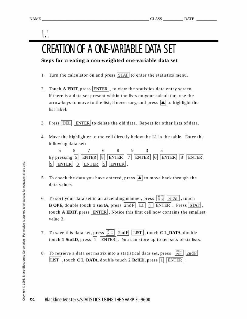
Steps for creating a non-weighted one-variable data set
1. Turn the calculator on and press STAT to enter the statistics menu.
2. Touch A EDIT, press ENTER , to view the statistics data entry screen.
If there is a data set present within the lists on your calculator, use the
arrow keys to move to the list, if necessary, and press ▲ to highlight the
list label.
3. Press DEL ENTER to delete the old data. Repeat for other lists of data.
4. Move the highlighter to the cell directly below the L1 in the table. Enter the
following data set:
5 8 7 6 8 9 3 5
by pressing 5 ENTER 8 ENTER 7 ENTER 6 ENTER 8 ENTER
9 ENTER 3 ENTER 5 ENTER .
5. To check the data you have entered, press ▲ to move back through the
data values.
6. To sort your data set in an ascending manner, press STAT , touch
B OPE, double touch 1 sortA, press 2ndF L1 ) ENTER . Press STAT ,
touch A EDIT, press ENTER . Notice this first cell now contains the smallest
value 3.
7. To save this data set, press 2ndF LIST , touch C L_DATA, double
touch 1 StoLD, press 1 ENTER . You can store up to ten sets of six lists.
8. To retrieve a data set matrix into a statistical data set, press 2ndF
LIST , touch C L_DATA, double touch 2 RclLD, press 1 ENTER .
CREATION OF A ONE-VARIABLE DATA SET 1.1
NAME _____________________________________________________ CLASS __________ DATE __________
×+ –
÷
×+ –
÷
×+ –
÷
Blackline Masters/STATISTICS USING THE SHARP EL-9600 57 Cop
yrig
ht ©
1998
, S
harp
Ele
ctro
nics
Cor
pora
tion.
Per
mis
sion
is g
rant
ed t
o ph
otoc
opy
for
educ
atio
nal u
se o
nly.
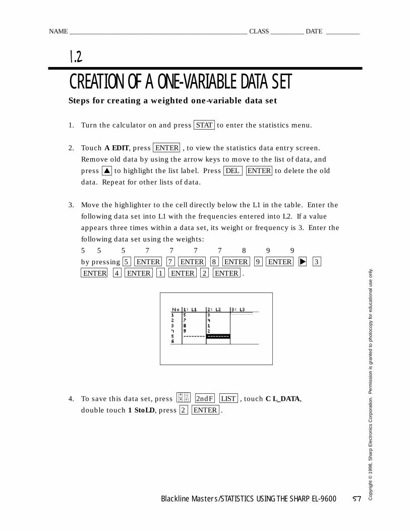
Steps for creating a weighted one-variable data set
1. Turn the calculator on and press STAT to enter the statistics menu.
2. Touch A EDIT, press ENTER , to view the statistics data entry screen.
Remove old data by using the arrow keys to move to the list of data, and
press ▲ to highlight the list label. Press DEL ENTER to delete the old
data. Repeat for other lists of data.
3. Move the highlighter to the cell directly below the L1 in the table. Enter the
following data set into L1 with the frequencies entered into L2. If a value
appears three times within a data set, its weight or frequency is 3. Enter the
following data set using the weights:
5 5 5 7 7 7 7 8 9 9
by pressing 5 ENTER 7 ENTER 8 ENTER 9 ENTER 3
ENTER 4 ENTER 1 ENTER 2 ENTER .
4. To save this data set, press 2ndF LIST , touch C L_DATA,
double touch 1 StoLD, press 2 ENTER .
CREATION OF A ONE-VARIABLE DATA SET1.2
NAME _____________________________________________________ CLASS __________ DATE __________
▼
×+ –
÷
58 Blackline Masters/STATISTICS USING THE SHARP EL-9600Cop
yrig
ht ©
1998
, S
harp
Ele
ctro
nics
Cor
pora
tion.
Per
mis
sion
is g
rant
ed t
o ph
otoc
opy
for
educ
atio
nal u
se o
nly.
Activity 1 Creating a non-weighted one-variable data set
1. Turn the calculator on and press STAT to enter the statistics menu.
2. Touch A EDIT, press ENTER , to view the statistics data entry screen.
If there is a data set present within the lists on your calculator, use the
arrow keys to move to the list, if necessary, and press ▲ to highlight the
list label.
3. Enter the following data set:
6 9 8 7 5 10 4 6
4. Check the data you have entered.
5. Sort the data in an ascending manner by pressing STAT , touch
B OPE, double touch 1 sortA, press 2ndF L1 ) ENTER . Press STAT ,
touch A EDIT, press ENTER .
6. Save this data set within L_DATA 3.
Activity 2 Creating a weighted one-variable data set
1. Enter the STAT menu and delete the old data set.
2. Enter the data values and frequency of occurrence.
Enter the following data set using the frequencies.
6 6 8 8 8 9 9 9 9
3, Check the data you have entered.
4. Save this data set within L_DATA 4.
CREATION OF A ONE-VARIABLE DATA SET 1.3
NAME _____________________________________________________ CLASS __________ DATE __________
×+ –
÷
Blackline Masters/STATISTICS USING THE SHARP EL-9600 59 Cop
yrig
ht ©
1998
, S
harp
Ele
ctro
nics
Cor
pora
tion.
Per
mis
sion
is g
rant
ed t
o ph
otoc
opy
for
educ
atio
nal u
se o
nly.
Steps for calculating numerical descriptions of a one-variable non-weighted data set1. Turn the calculator on and press STAT to enter the statistics menu.
Touch A EDIT, press ENTER , to view the statistics data entry screen.
If there is a data set present within the lists on your calculator, use the
arrow keys to move to the list, if necessary, and press ▲ to highlight the
list label. Press DEL ENTER to delete the old data. Repeat for other lists
of data.
2. Move the highlighter to the cell directly below the L1 in the table.
Enter the following data set:
25 32 28 33 31 27 40 38 29 30
3. Check the data you have entered and correct any errors you may find.
Press 2ndF QUIT to exit the data entry screen. To calculate the numerical
descriptions of the data set, press STAT , touch C CALC, and double touch
1 1_Stats. Press ENTER and the statistical results will appear.
4. The statistics displayed are:
1. the average or mean value of the data set, ;
2. the standard deviation assuming the data set is a sample from a
population, sx;
3. the standard deviation assuming the data set represents the entire
population, σx;
4. the sum of the data values, ∑x;
5. the sum of the squared data values, ∑x2;
6. the number of values in the data set, n;
Press ▼ four times to see the rest of the statistics.
7. the minimum value in the data set, xmin;
8. the first quartile (25th percentile), Q1;
9. the median (50th percentile), Med;
10. the third quartile (75th percentile), Q3; and
11. the maximum value in the data set, xmax.2.2
NUMERICAL DESCRIPTION OF A ONE-VARIABLE DATA SET
2.1
NAME _____________________________________________________ CLASS __________ DATE __________
x
60 Blackline Masters/STATISTICS USING THE SHARP EL-9600Cop
yrig
ht ©
1998
, S
harp
Ele
ctro
nics
Cor
pora
tion.
Per
mis
sion
is g
rant
ed t
o ph
otoc
opy
for
educ
atio
nal u
se o
nly.
Steps for calculating numerical descriptions of a one-variableweighted data set
1. Turn the calculator on and press STAT to enter the statistics menu.
Touch A EDIT, press ENTER , to view the statistics data entry screen.
If there is a data set present within the lists on your calculator, use the
arrow keys to move to the list, if necessary, and press ▲ to highlight the
list label. Press DEL ENTER to delete the old data. Repeat for other
lists of data.
2. Move the highlighter to the cell directly below the L1 in the table. Enter the
following data set generated by rolling a die fifty times.
Value Frequency
1 8
2 10
3 12
4 9
5 6
6 5
Remember to enter the frequencies in L2.
3. Check the data you have entered and correct any errors you may find.
Press 2ndF QUIT to exit the data entry screen. To calculate the numerical
descriptions of the data set, press STAT , touch C CALC, double touch
1 1_Stats, and press 2ndF L1 , 2ndF L2 . Press ENTER and the
statistical results will appear.
NUMERICAL DESCRIPTION OF A ONE-VARIABLE DATA SET
2.2
NAME _____________________________________________________ CLASS __________ DATE __________
Blackline Masters/STATISTICS USING THE SHARP EL-9600 61 Cop
yrig
ht ©
1998
, S
harp
Ele
ctro
nics
Cor
pora
tion.
Per
mis
sion
is g
rant
ed t
o ph
otoc
opy
for
educ
atio
nal u
se o
nly.
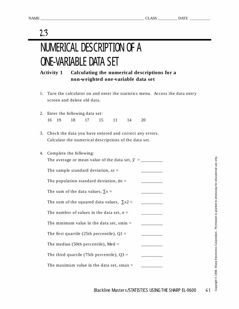
Activity 1 Calculating the numerical descriptions for a non-weighted one-variable data set
1. Turn the calculator on and enter the statistics menu. Access the data entry
screen and delete old data.
2. Enter the following data set:
16 19 18 17 15 11 14 20
3. Check the data you have entered and correct any errors.
Calculate the numerical descriptions of the data set.
4. Complete the following:
The average or mean value of the data set, = __________
The sample standard deviation, sx = __________
The population standard deviation, σx = __________
The sum of the data values, ∑x = __________
The sum of the squared data values, ∑x2 = __________
The number of values in the data set, n = __________
The minimum value in the data set, xmin = __________
The first quartile (25th percentile), Q1 = __________
The median (50th percentile), Med = __________
The third quartile (75th percentile), Q3 = __________
The maximum value in the data set, xmax = __________
NUMERICAL DESCRIPTION OF A ONE-VARIABLE DATA SET
2.3
NAME _____________________________________________________ CLASS __________ DATE __________
x
62 Blackline Masters/STATISTICS USING THE SHARP EL-9600Cop
yrig
ht ©
1998
, S
harp
Ele
ctro
nics
Cor
pora
tion.
Per
mis
sion
is g
rant
ed t
o ph
otoc
opy
for
educ
atio
nal u
se o
nly.
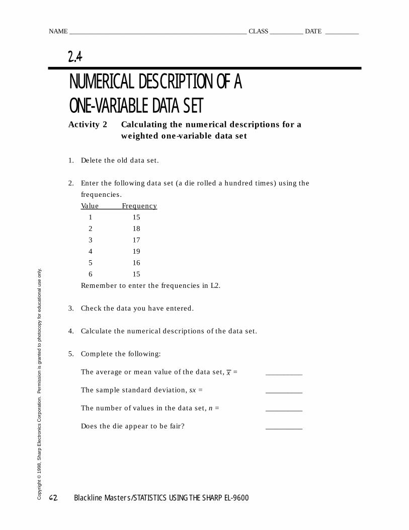
Activity 2 Calculating the numerical descriptions for a weighted one-variable data set
1. Delete the old data set.
2. Enter the following data set (a die rolled a hundred times) using the
frequencies.
Value Frequency
1 15
2 18
3 17
4 19
5 16
6 15
Remember to enter the frequencies in L2.
3. Check the data you have entered.
4. Calculate the numerical descriptions of the data set.
5. Complete the following:
The average or mean value of the data set, = __________
The sample standard deviation, sx = __________
The number of values in the data set, n = __________
Does the die appear to be fair? __________
NUMERICAL DESCRIPTION OF A ONE-VARIABLE DATA SET
2.4
NAME _____________________________________________________ CLASS __________ DATE __________
x
Blackline Masters/STATISTICS USING THE SHARP EL-9600 63 Cop
yrig
ht ©
1998
, S
harp
Ele
ctro
nics
Cor
pora
tion.
Per
mis
sion
is g
rant
ed t
o ph
otoc
opy
for
educ
atio
nal u
se o
nly.
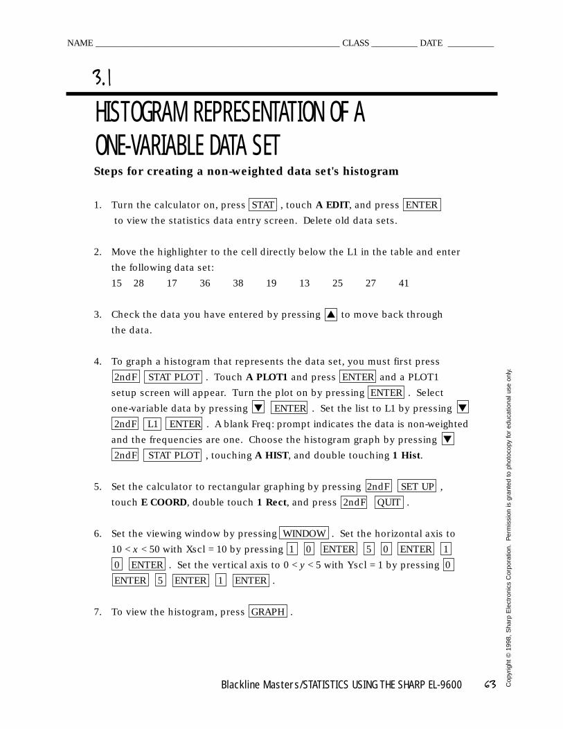
Steps for creating a non-weighted data set's histogram
1. Turn the calculator on, press STAT , touch A EDIT, and press ENTER
to view the statistics data entry screen. Delete old data sets.
2. Move the highlighter to the cell directly below the L1 in the table and enter
the following data set:
15 28 17 36 38 19 13 25 27 41
3. Check the data you have entered by pressing ▲ to move back through
the data.
4. To graph a histogram that represents the data set, you must first press
2ndF STAT PLOT . Touch A PLOT1 and press ENTER and a PLOT1
setup screen will appear. Turn the plot on by pressing ENTER . Select
one-variable data by pressing ▼ ENTER . Set the list to L1 by pressing ▼
2ndF L1 ENTER . A blank Freq: prompt indicates the data is non-weighted
and the frequencies are one. Choose the histogram graph by pressing ▼
2ndF STAT PLOT , touching A HIST, and double touching 1 Hist.
5. Set the calculator to rectangular graphing by pressing 2ndF SET UP ,
touch E COORD, double touch 1 Rect, and press 2ndF QUIT .
6. Set the viewing window by pressing WINDOW . Set the horizontal axis to
10 < x < 50 with Xscl = 10 by pressing 1 0 ENTER 5 0 ENTER 1
0 ENTER . Set the vertical axis to 0 < y < 5 with Yscl = 1 by pressing 0
ENTER 5 ENTER 1 ENTER .
7. To view the histogram, press GRAPH .
HISTOGRAM REPRESENTATION OF A ONE-VARIABLE DATA SET
3.1
NAME _____________________________________________________ CLASS __________ DATE __________
64 Blackline Masters/STATISTICS USING THE SHARP EL-9600Cop
yrig
ht ©
1998
, S
harp
Ele
ctro
nics
Cor
pora
tion.
Per
mis
sion
is g
rant
ed t
o ph
otoc
opy
for
educ
atio
nal u
se o
nly.
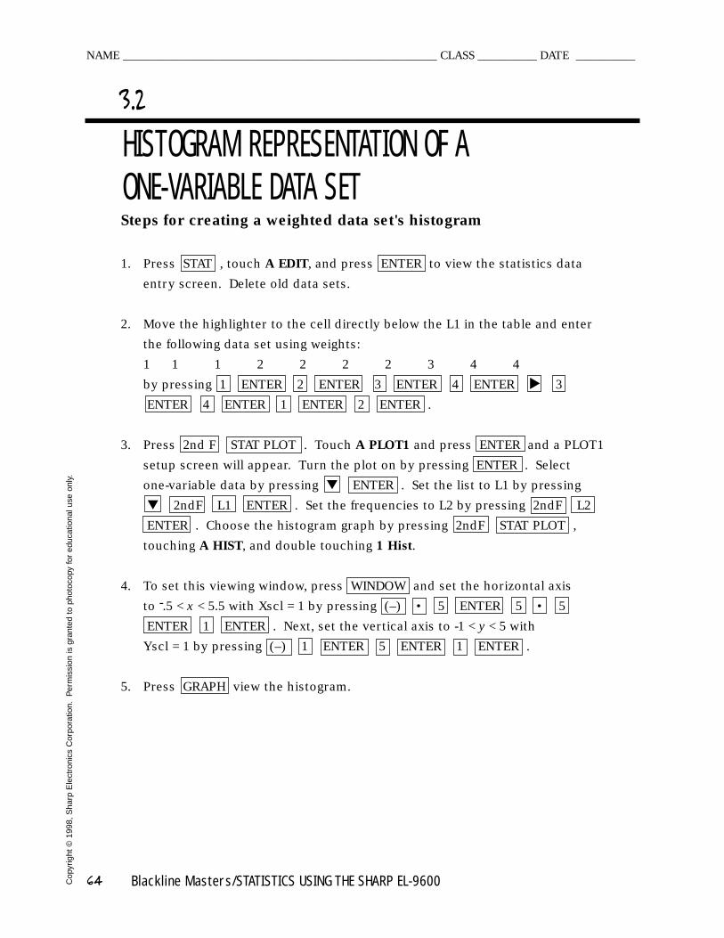
Steps for creating a weighted data set's histogram
1. Press STAT , touch A EDIT, and press ENTER to view the statistics data
entry screen. Delete old data sets.
2. Move the highlighter to the cell directly below the L1 in the table and enter
the following data set using weights:
1 1 1 2 2 2 2 3 4 4
by pressing 1 ENTER 2 ENTER 3 ENTER 4 ENTER 3
ENTER 4 ENTER 1 ENTER 2 ENTER .
3. Press 2nd F STAT PLOT . Touch A PLOT1 and press ENTER and a PLOT1
setup screen will appear. Turn the plot on by pressing ENTER . Select
one-variable data by pressing ▼ ENTER . Set the list to L1 by pressing
▼ 2ndF L1 ENTER . Set the frequencies to L2 by pressing 2ndF L2
ENTER . Choose the histogram graph by pressing 2ndF STAT PLOT ,
touching A HIST, and double touching 1 Hist.
4. To set this viewing window, press WINDOW and set the horizontal axis
to -.5 < x < 5.5 with Xscl = 1 by pressing (–) • 5 ENTER 5 • 5
ENTER 1 ENTER . Next, set the vertical axis to -1 < y < 5 with
Yscl = 1 by pressing (–) 1 ENTER 5 ENTER 1 ENTER .
5. Press GRAPH view the histogram.
HISTOGRAM REPRESENTATION OF A ONE-VARIABLE DATA SET
3.2
NAME _____________________________________________________ CLASS __________ DATE __________
▼
Blackline Masters/STATISTICS USING THE SHARP EL-9600 65 Cop
yrig
ht ©
1998
, S
harp
Ele
ctro
nics
Cor
pora
tion.
Per
mis
sion
is g
rant
ed t
o ph
otoc
opy
for
educ
atio
nal u
se o
nly.
Activity 1 Creating a non-weighted data set's histogram
1. Turn the calculator on and enter the statistics menu.
2. Delete old data.
3. Enter the following data set:
113 126 115 134 136 117 111 123 125 139
4. Set the STAT PLOT for a histogram.
5. Set the viewing window to 110 < x < 140 with Xscl = 10, and setting the
vertical axis to 0 < y < 5 with Yscl = 1.
6. Press GRAPH to view the histogram.
Activity 2 Creating a weighted data set's histogram
1. Enter the statistics menu.
2. Delete old data.
3. Enter the following data set using the weights:
11 11 12 12 12 13 13 13 13 14
4. Set the STAT PLOT for a histogram with frequencies in L2.
5. Set the viewing window to 9.5 < x < 15.5 with Xscl = 1, and
set the Y range to -1 < y < 5 with Yscl = 1.
6. Press GRAPH to view the histogram.
HISTOGRAM REPRESENTATION OF A ONE-VARIABLE DATA SET
3.3
NAME _____________________________________________________ CLASS __________ DATE __________
66 Blackline Masters/STATISTICS USING THE SHARP EL-9600Cop
yrig
ht ©
1998
, S
harp
Ele
ctro
nics
Cor
pora
tion.
Per
mis
sion
is g
rant
ed t
o ph
otoc
opy
for
educ
atio
nal u
se o
nly.
Steps for creating a non-weighted data set's broken-line graph
1. Turn the calculator on and press STAT to enter the statistics menu.
Delete old data and enter the following data set for L1:
15 28 17 36 38 19 13 25 27 41
2. Check the data you have entered by pressing ▲ to move back through
the data.
3. To graph a broken-line graph for the data set, first press 2ndF STAT PLOT ,
touch A PLOT1, and press ENTER . Turn PLOT1 on by pressing ENTER .
Press ▼ ENTER to choose one-variable data. Press ▼ 2ndF L1
ENTER to enter L1 as the data list. Clear the frequency prompt by pressing
DEL ENTER . Set the graph to a broken line graph by pressing 2ndF
STAT PLOT , touch B B.L., and double touch 3 Broken .
4. In our example, the smallest value is 13 and the largest value is 41.
The logical intervals for the data set would be 10-19 (tens), 20-29 (twenties),
30-39 (thirties), and 40-49 (forties). To set this viewing window, press
WINDOW and set the horizontal axis to 10 < x < 50 with Xscl = 10.
Set the vertical axis to 0 < y < 5 with Yscl = 1.
5. To view the graph, press GRAPH .
6. Press TRACE and then press repeatedly to trace the points making up
the broken-line graph.
7. Turn PLOT1 off by pressing 2ndF STAT PLOT ENTER ENTER
2ndF QUIT .
OTHER GRAPHICAL PORTRAYALS OF A ONE-VARIABLE DATA SET
4.1
NAME _____________________________________________________ CLASS __________ DATE __________
▼
▼
▼
Blackline Masters/STATISTICS USING THE SHARP EL-9600 67 Cop
yrig
ht ©
1998
, S
harp
Ele
ctro
nics
Cor
pora
tion.
Per
mis
sion
is g
rant
ed t
o ph
otoc
opy
for
educ
atio
nal u
se o
nly.
Steps for creating a weighted data set's box-and-whisker chart
1. Press STAT to enter the statistics menu. Delete old data and enter the
following data set in L1 using weights in L2:
1 1 1 2 2 2 2 3 4 4
2. To construct a box-and-whisker chart, first press 2ndF STAT PLOT
ENTER . Press ENTER to turn PLOT1 on. Press ▼ ENTER to choose
one-variable data. Press ▼ 2ndF L1 ENTER to enter L1 as the data
list. Set the frequency prompt to L2 by pressing 2ndF L2 ENTER .
Set the graph to a broken-line graph by pressing 2ndF STAT PLOT ,
touch E BOX, and double touch 1 Box.
3. In the example, the data is discrete with a smallest value of 1 and a largest
value of 4. Set the viewing window to 0 < x < 5 with Xscl = 1. Next, set the
vertical axis to 0 < y < 1 with Yscl = 1.
4. To view the box-and-whisker chart for the data, press GRAPH .
5. Press TRACE followed by and to view the five values making up the
box-and whisker chart.
6. Turn PLOT1 off by pressing 2ndF STAT PLOT ENTER ENTER
2ndF QUIT .
OTHER GRAPHICAL PORTRAYALS OF A ONE-VARIABLE DATA SET
4.2
NAME _____________________________________________________ CLASS __________ DATE __________
▼
▼
▼
68 Blackline Masters/STATISTICS USING THE SHARP EL-9600Cop
yrig
ht ©
1998
, S
harp
Ele
ctro
nics
Cor
pora
tion.
Per
mis
sion
is g
rant
ed t
o ph
otoc
opy
for
educ
atio
nal u
se o
nly.
Activity 1 Creating a non-weighted data set's broken-line graph
1. Turn the calculator on and enter the statistics menu.
2. Delete the old data set.
3. Enter the following data set in L1:
113 126 115 134 136 117 111 123 125 139
4. Set PLOT1 to a broken-line graph.
5. Set the viewing window with a horizontal axis of 110 < x < 140 and Xscl = 10.
Set the vertical axis to 0 < y < 5 with Yscl = 1.
6. Press GRAPH to display the broken line graph.
Activity 2 Creating a weighted data set's box-and-whisker chart
1. Enter the statistics menu.
2. Delete the old data set.
3. Enter the following data set in L1 with the weights in L2:
11 11 12 12 12 13 13 13 13 14
4. Set PLOT1 to a box-and-whisker chart.
5. Set the viewing window to 10 < x < 15 with Xscl = 1, and 0 < y < 1 with Yscl = 1.
6. Press GRAPH to display the box-and-whisker chart.
OTHER GRAPHICAL PORTRAYALS OF A ONE-VARIABLE DATA SET
4.3
NAME _____________________________________________________ CLASS __________ DATE __________
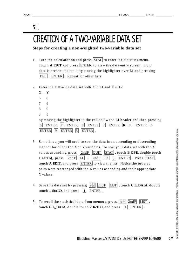
Blackline Masters/STATISTICS USING THE SHARP EL-9600 69 Cop
yrig
ht ©
1998
, S
harp
Ele
ctro
nics
Cor
pora
tion.
Per
mis
sion
is g
rant
ed t
o ph
otoc
opy
for
educ
atio
nal u
se o
nly.
Steps for creating a non-weighted two-variable data set
1. Turn the calculator on and press STAT to enter the statistics menu.
Touch A EDIT and press ENTER to view the data-entry screen. If old
data is present, delete it by moving the highlighter over L1 and pressing
DEL ENTER . Repeat for other lists.
2. Enter the following data set with X in L1 and Y in L2:
X Y
5 8
7 6
8 9
3 5
by moving the highlighter to the cell below the L1 header and then pressing
5 ENTER 7 ENTER 8 ENTER 3 ENTER 8 ENTER 6
ENTER 9 ENTER 5 ENTER .
3. Sometimes, you will need to sort the data in an ascending or descending
manner for either the X or Y variables. To sort your data set with the X
values ascending, press 2ndF QUIT STAT , touch B OPE, double touch
1 sortA(, press 2ndF L1 , 2ndF L2 ) ENTER . Press STAT ,
touch A EDIT, and press ENTER to view the list. Notice the ordered
pairs were rearranged with the X values ascending and their appropriate
Y values.
4. Save this data set by pressing 2ndF LIST , touch C L_DATA, double
touch 1 StoLD, and press 1 ENTER .
5. To recall the statistical data from memory, press 2ndF LIST ,
touch C L_DATA, double touch 2 RclLD, and press 1 ENTER .
CREATION OF A TWO-VARIABLE DATA SET 5.1
NAME _____________________________________________________ CLASS __________ DATE __________
▼
×+ –
÷
×+ –
÷
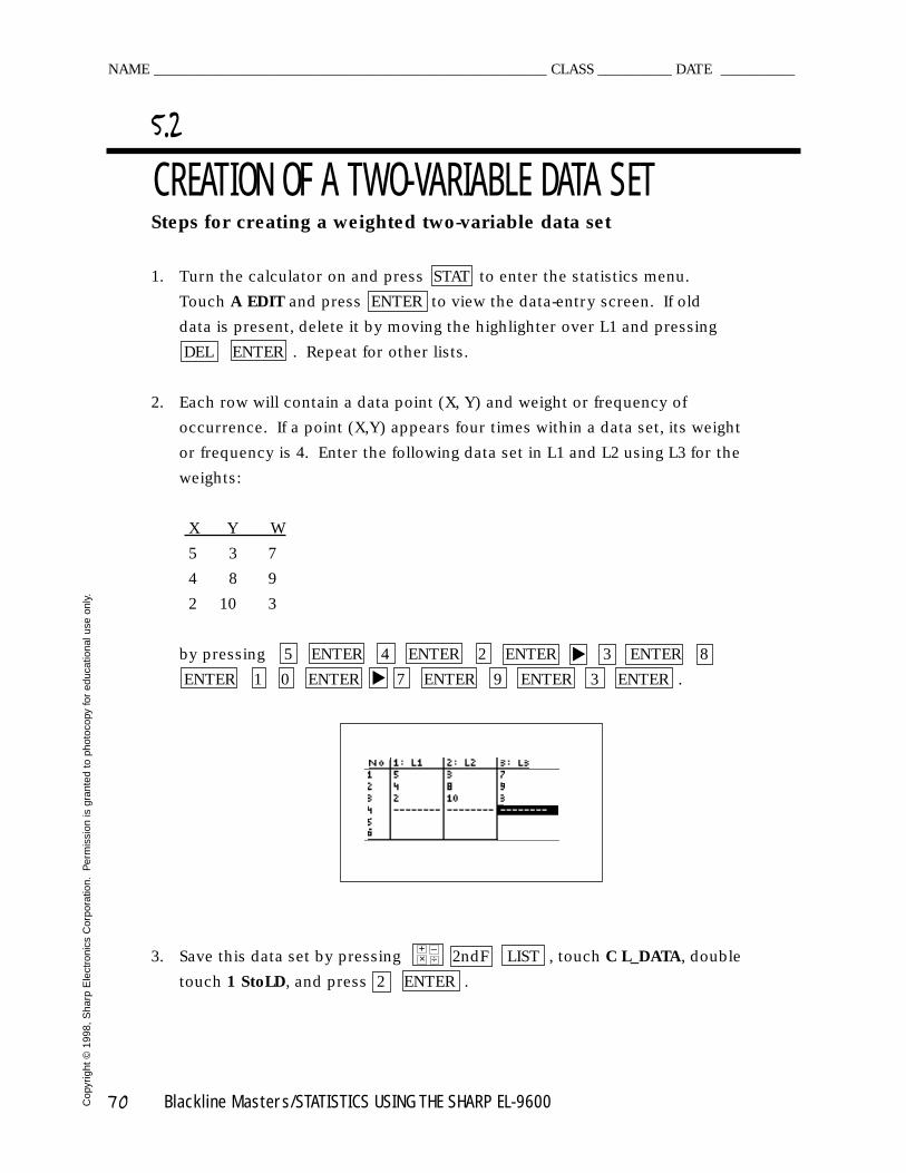
70 Blackline Masters/STATISTICS USING THE SHARP EL-9600Cop
yrig
ht ©
1998
, S
harp
Ele
ctro
nics
Cor
pora
tion.
Per
mis
sion
is g
rant
ed t
o ph
otoc
opy
for
educ
atio
nal u
se o
nly.
Steps for creating a weighted two-variable data set
1. Turn the calculator on and press STAT to enter the statistics menu.
Touch A EDIT and press ENTER to view the data-entry screen. If old
data is present, delete it by moving the highlighter over L1 and pressing
DEL ENTER . Repeat for other lists.
2. Each row will contain a data point (X, Y) and weight or frequency of
occurrence. If a point (X,Y) appears four times within a data set, its weight
or frequency is 4. Enter the following data set in L1 and L2 using L3 for the
weights:
X Y W
5 3 7
4 8 9
2 10 3
by pressing 5 ENTER 4 ENTER 2 ENTER 3 ENTER 8
ENTER 1 0 ENTER 7 ENTER 9 ENTER 3 ENTER .
3. Save this data set by pressing 2ndF LIST , touch C L_DATA, double
touch 1 StoLD, and press 2 ENTER .
CREATION OF A TWO-VARIABLE DATA SET 5.2
NAME _____________________________________________________ CLASS __________ DATE __________
▼
▼
×+ –
÷
Blackline Masters/STATISTICS USING THE SHARP EL-9600 71 Cop
yrig
ht ©
1998
, S
harp
Ele
ctro
nics
Cor
pora
tion.
Per
mis
sion
is g
rant
ed t
o ph
otoc
opy
for
educ
atio
nal u
se o
nly.
Activity 1 Creating a non-weighted two-variable data set
1. Turn the calculator on and enter the statistics menu.
2. Delete old data.
3. Enter the following data set:
X Y
6 9
8 7
5 10
4 6
4. Check the data you have entered.
5. Sort the data in an ascending manner.
6. Save this data set within list data 1.
Activity 2 Creating a weighted two-variable data set
1. Delete the old data set.
2. Enter the following data set using the frequencies.
X Y W
6 6 8
8 8 9
9 9 10
3. Check the data you have entered.
4. Save this data set within list data 2.
CREATION OF A TWO-VARIABLE DATA SET 5.3
NAME _____________________________________________________ CLASS __________ DATE __________
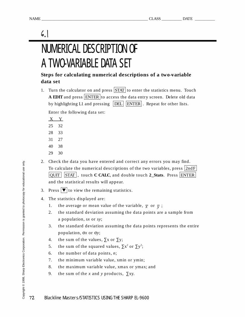
72 Blackline Masters/STATISTICS USING THE SHARP EL-9600Cop
yrig
ht ©
1998
, S
harp
Ele
ctro
nics
Cor
pora
tion.
Per
mis
sion
is g
rant
ed t
o ph
otoc
opy
for
educ
atio
nal u
se o
nly.
Steps for calculating numerical descriptions of a two-variable data set
1. Turn the calculator on and press STAT to enter the statistics menu. Touch
A EDIT and press ENTER to access the data entry screen. Delete old data
by highlighting L1 and pressing DEL ENTER . Repeat for other lists.
Enter the following data set:
X Y
25 32
28 33
31 27
40 38
29 30
2. Check the data you have entered and correct any errors you may find.
To calculate the numerical descriptions of the two variables, press 2ndF
QUIT STAT , touch C CALC, and double touch 2_Stats. Press ENTER
and the statistical results will appear.
3. Press ▼ to view the remaining statistics.
4. The statistics displayed are:
1. the average or mean value of the variable, or ;
2. the standard deviation assuming the data points are a sample from
a population, sx or sy;
3. the standard deviation assuming the data points represents the entire
population, σx or σy;
4. the sum of the values, ∑x or ∑y;
5. the sum of the squared values, ∑x2 or ∑y2;
6. the number of data points, n;
7. the minimum variable value, xmin or ymin;
8. the maximum variable value, xmax or ymax; and
9. the sum of the x and y products, ∑xy.
NUMERICAL DESCRIPTION OF A TWO-VARIABLE DATA SET
6.1
NAME _____________________________________________________ CLASS __________ DATE __________
x y
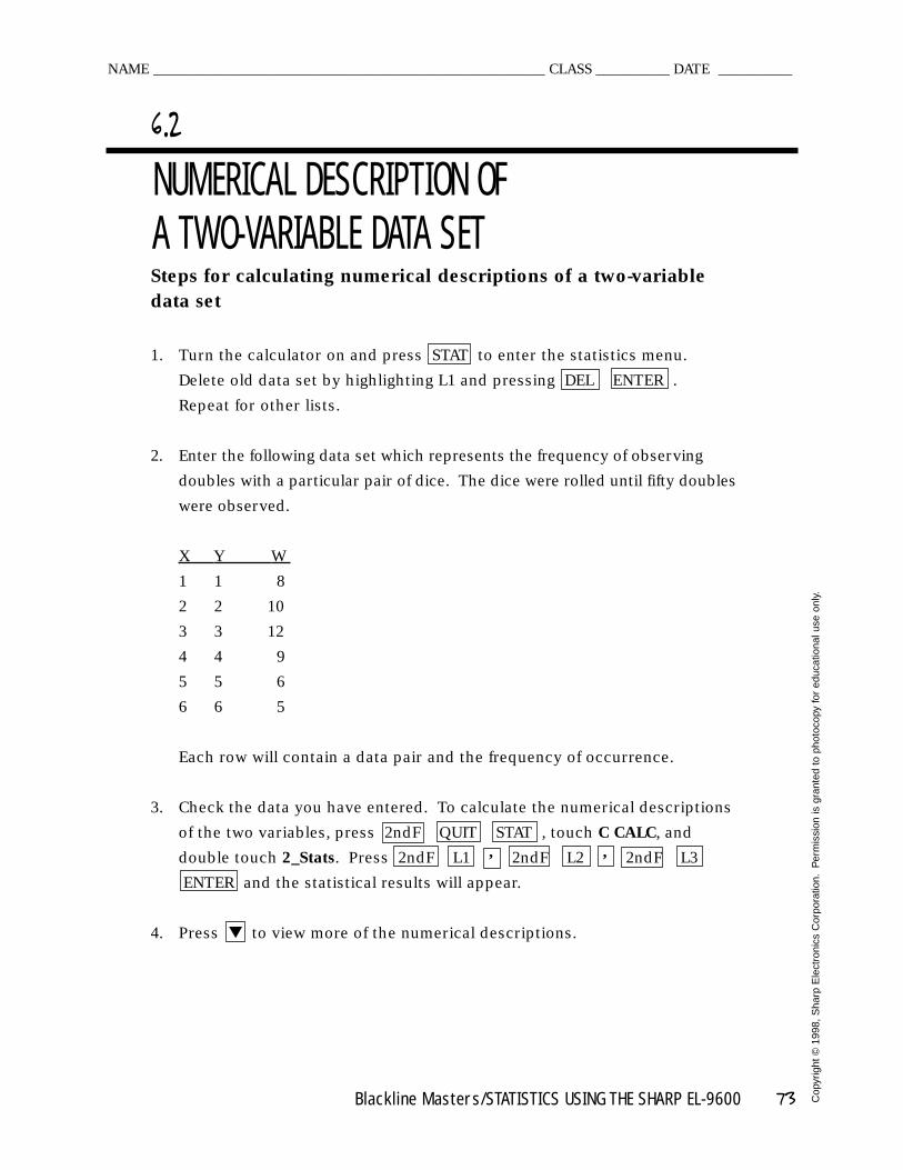
Blackline Masters/STATISTICS USING THE SHARP EL-9600 73 Cop
yrig
ht ©
1998
, S
harp
Ele
ctro
nics
Cor
pora
tion.
Per
mis
sion
is g
rant
ed t
o ph
otoc
opy
for
educ
atio
nal u
se o
nly.
Steps for calculating numerical descriptions of a two-variable data set
1. Turn the calculator on and press STAT to enter the statistics menu.
Delete old data set by highlighting L1 and pressing DEL ENTER .
Repeat for other lists.
2. Enter the following data set which represents the frequency of observing
doubles with a particular pair of dice. The dice were rolled until fifty doubles
were observed.
X Y W
1 1 8
2 2 10
3 3 12
4 4 9
5 5 6
6 6 5
Each row will contain a data pair and the frequency of occurrence.
3. Check the data you have entered. To calculate the numerical descriptions
of the two variables, press 2ndF QUIT STAT , touch C CALC, and
double touch 2_Stats. Press 2ndF L1 , 2ndF L2 , 2ndF L3
ENTER and the statistical results will appear.
4. Press ▼ to view more of the numerical descriptions.
NUMERICAL DESCRIPTION OF A TWO-VARIABLE DATA SET
6.2
NAME _____________________________________________________ CLASS __________ DATE __________
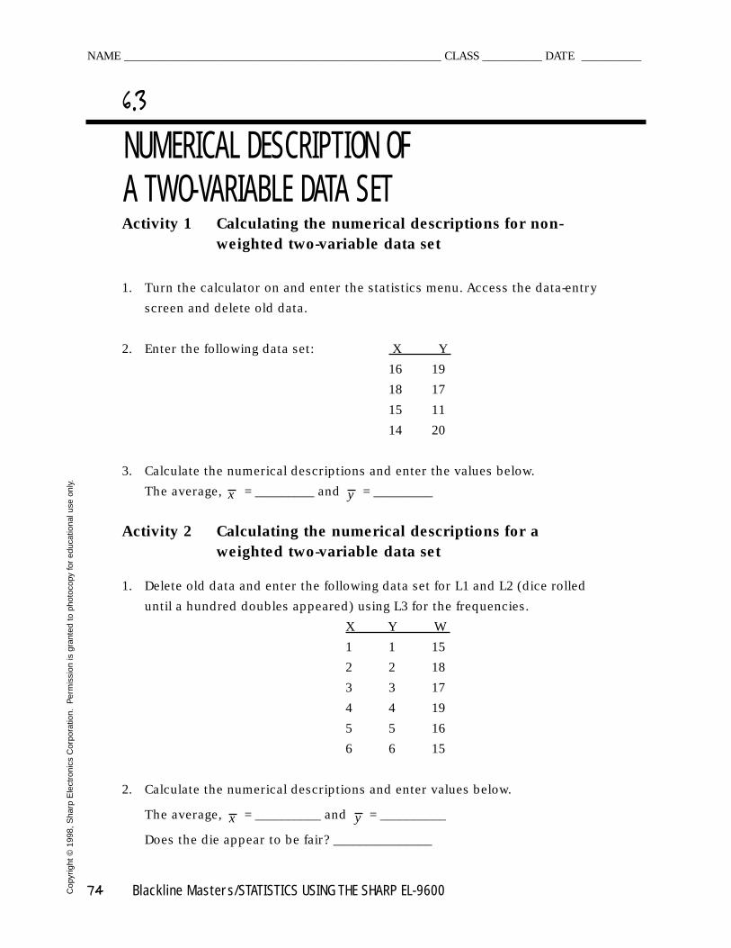
74 Blackline Masters/STATISTICS USING THE SHARP EL-9600Cop
yrig
ht ©
1998
, S
harp
Ele
ctro
nics
Cor
pora
tion.
Per
mis
sion
is g
rant
ed t
o ph
otoc
opy
for
educ
atio
nal u
se o
nly.
Activity 1 Calculating the numerical descriptions for non-weighted two-variable data set
1. Turn the calculator on and enter the statistics menu. Access the data-entry
screen and delete old data.
2. Enter the following data set: X Y
16 19
18 17
15 11
14 20
3. Calculate the numerical descriptions and enter the values below.
The average, = _________ and = _________
Activity 2 Calculating the numerical descriptions for a weighted two-variable data set
1. Delete old data and enter the following data set for L1 and L2 (dice rolled
until a hundred doubles appeared) using L3 for the frequencies.
X Y W
1 1 15
2 2 18
3 3 17
4 4 19
5 5 16
6 6 15
2. Calculate the numerical descriptions and enter values below.
The average, = __________ and = __________
Does the die appear to be fair? _______________
NUMERICAL DESCRIPTION OF A TWO-VARIABLE DATA SET
6.3
NAME _____________________________________________________ CLASS __________ DATE __________
x y
x y
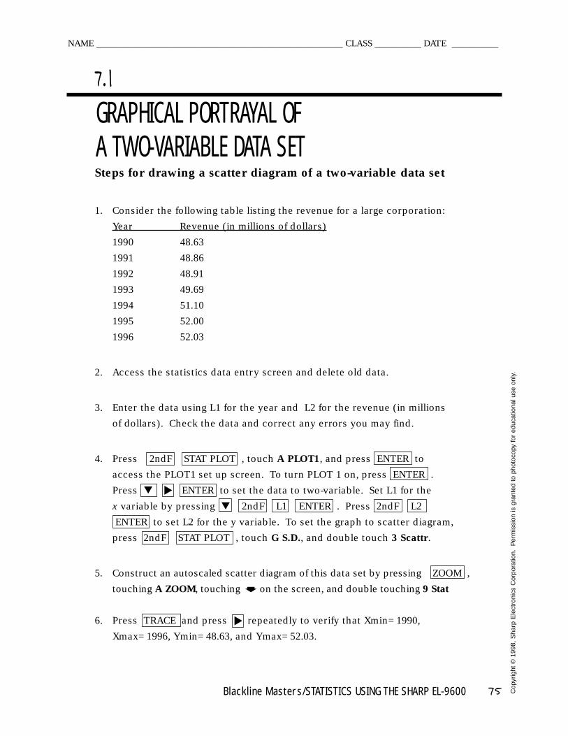
Blackline Masters/STATISTICS USING THE SHARP EL-9600 75 Cop
yrig
ht ©
1998
, S
harp
Ele
ctro
nics
Cor
pora
tion.
Per
mis
sion
is g
rant
ed t
o ph
otoc
opy
for
educ
atio
nal u
se o
nly.
Steps for drawing a scatter diagram of a two-variable data set
1. Consider the following table listing the revenue for a large corporation:
Year Revenue (in millions of dollars)
1990 48.63
1991 48.86
1992 48.91
1993 49.69
1994 51.10
1995 52.00
1996 52.03
2. Access the statistics data entry screen and delete old data.
3. Enter the data using L1 for the year and L2 for the revenue (in millions
of dollars). Check the data and correct any errors you may find.
4. Press 2ndF STAT PLOT , touch A PLOT1, and press ENTER to
access the PLOT1 set up screen. To turn PLOT 1 on, press ENTER .
Press ▼ ENTER to set the data to two-variable. Set L1 for the
x variable by pressing ▼ 2ndF L1 ENTER . Press 2ndF L2
ENTER to set L2 for the y variable. To set the graph to scatter diagram,
press 2ndF STAT PLOT , touch G S.D., and double touch 3 Scattr.
5. Construct an autoscaled scatter diagram of this data set by pressing ZOOM ,
touching A ZOOM, touching on the screen, and double touching 9 Stat
6. Press TRACE and press repeatedly to verify that Xmin= 1990,
Xmax= 1996, Ymin= 48.63, and Ymax= 52.03.
GRAPHICAL PORTRAYAL OF A TWO-VARIABLE DATA SET
7.1
NAME _____________________________________________________ CLASS __________ DATE __________
▼
➧
▼
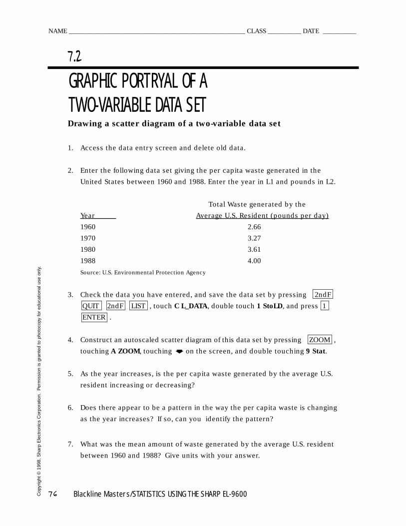
76 Blackline Masters/STATISTICS USING THE SHARP EL-9600Cop
yrig
ht ©
1998
, S
harp
Ele
ctro
nics
Cor
pora
tion.
Per
mis
sion
is g
rant
ed t
o ph
otoc
opy
for
educ
atio
nal u
se o
nly.
Drawing a scatter diagram of a two-variable data set
1. Access the data entry screen and delete old data.
2. Enter the following data set giving the per capita waste generated in the
United States between 1960 and 1988. Enter the year in L1 and pounds in L2.
Total Waste generated by the
Year Average U.S. Resident (pounds per day)
1960 2.66
1970 3.27
1980 3.61
1988 4.00
Source: U.S. Environmental Protection Agency
3. Check the data you have entered, and save the data set by pressing 2ndF
QUIT 2ndF LIST , touch C L_DATA, double touch 1 StoLD, and press 1
ENTER .
4. Construct an autoscaled scatter diagram of this data set by pressing ZOOM ,
touching A ZOOM, touching on the screen, and double touching 9 Stat.
5. As the year increases, is the per capita waste generated by the average U.S.
resident increasing or decreasing?
6. Does there appear to be a pattern in the way the per capita waste is changing
as the year increases? If so, can you identify the pattern?
7. What was the mean amount of waste generated by the average U.S. resident
between 1960 and 1988? Give units with your answer.
GRAPHIC PORTRYAL OF A TWO-VARIABLE DATA SET
7.2
NAME _____________________________________________________ CLASS __________ DATE __________
➧
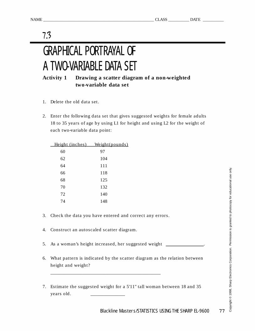
Blackline Masters/STATISTICS USING THE SHARP EL-9600 77 Cop
yrig
ht ©
1998
, S
harp
Ele
ctro
nics
Cor
pora
tion.
Per
mis
sion
is g
rant
ed t
o ph
otoc
opy
for
educ
atio
nal u
se o
nly.
Activity 1 Drawing a scatter diagram of a non-weighted two-variable data set
1. Delete the old data set.
2. Enter the following data set that gives suggested weights for female adults
18 to 35 years of age by using L1 for height and using L2 for the weight of
each two-variable data point:
Height (inches) Weight(pounds)
60 97
62 104
64 111
66 118
68 125
70 132
72 140
74 148
3. Check the data you have entered and correct any errors.
4. Construct an autoscaled scatter diagram.
5. As a woman’s height increased, her suggested weight .
6. What pattern is indicated by the scatter diagram as the relation between
height and weight?
________________________________________________
7. Estimate the suggested weight for a 5'11" tall woman between 18 and 35
years old. _______________
GRAPHICAL PORTRAYAL OF A TWO-VARIABLE DATA SET
7.3
NAME _____________________________________________________ CLASS __________ DATE __________
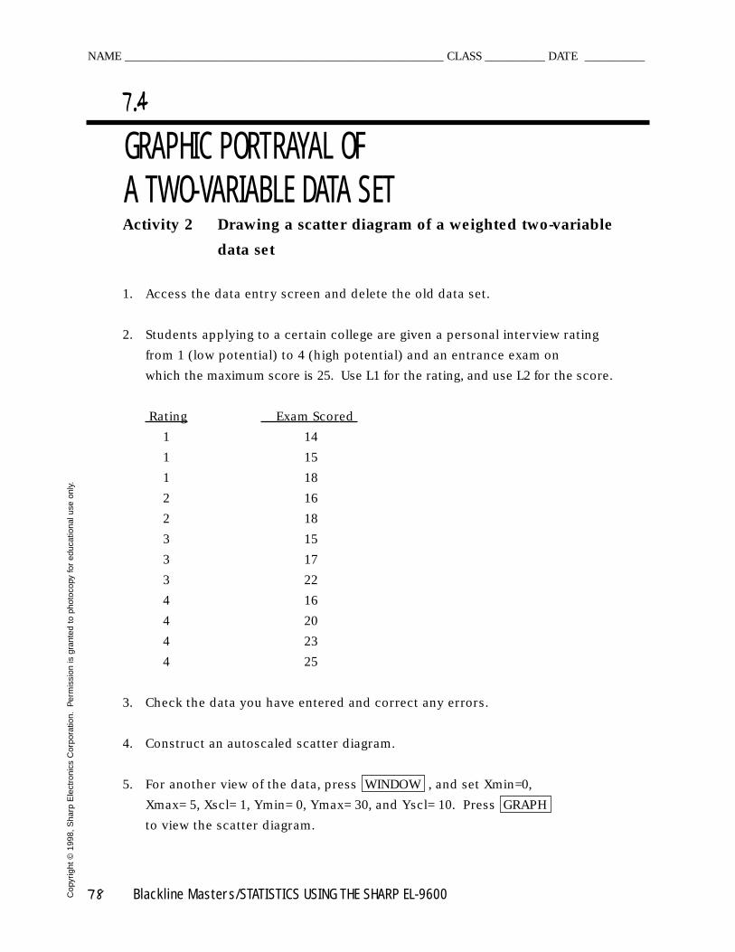
78 Blackline Masters/STATISTICS USING THE SHARP EL-9600Cop
yrig
ht ©
1998
, S
harp
Ele
ctro
nics
Cor
pora
tion.
Per
mis
sion
is g
rant
ed t
o ph
otoc
opy
for
educ
atio
nal u
se o
nly.
Activity 2 Drawing a scatter diagram of a weighted two-variable
data set
1. Access the data entry screen and delete the old data set.
2. Students applying to a certain college are given a personal interview rating
from 1 (low potential) to 4 (high potential) and an entrance exam on
which the maximum score is 25. Use L1 for the rating, and use L2 for the score.
Rating Exam Scored
1 14
1 15
1 18
2 16
2 18
3 15
3 17
3 22
4 16
4 20
4 23
4 25
3. Check the data you have entered and correct any errors.
4. Construct an autoscaled scatter diagram.
5. For another view of the data, press WINDOW , and set Xmin=0,
Xmax= 5, Xscl= 1, Ymin= 0, Ymax= 30, and Yscl= 10. Press GRAPH
to view the scatter diagram.
GRAPHIC PORTRAYAL OF A TWO-VARIABLE DATA SET
7.4
NAME _____________________________________________________ CLASS __________ DATE __________
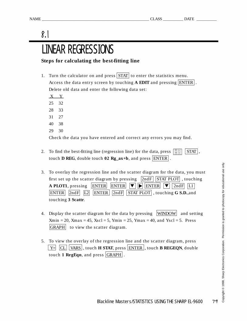
Blackline Masters/STATISTICS USING THE SHARP EL-9600 79 Cop
yrig
ht ©
1998
, S
harp
Ele
ctro
nics
Cor
pora
tion.
Per
mis
sion
is g
rant
ed t
o ph
otoc
opy
for
educ
atio
nal u
se o
nly.
Steps for calculating the best-fitting line
1. Turn the calculator on and press STAT to enter the statistics menu.
Access the data entry screen by touching A EDIT and pressing ENTER .
Delete old data and enter the following data set:
X Y
25 32
28 33
31 27
40 38
29 30
Check the data you have entered and correct any errors you may find.
2. To find the best-fitting line (regression line) for the data, press STAT ,
touch D REG, double touch 02 Rg_ax+b, and press ENTER .
3. To overlay the regression line and the scatter diagram for the data, you must
first set up the scatter diagram by pressing 2ndF STAT PLOT , touching
A PLOT1, pressing ENTER ENTER ▼ ENTER ▼ 2ndF L1
ENTER 2ndF L2 ENTER 2ndF STAT PLOT , touching G S.D.,and
touching 3 Scattr.
4. Display the scatter diagram for the data by pressing WINDOW and setting
Xmin = 20, Xmax = 45, Xscl = 5, Ymin = 25, Ymax = 40, and Yscl = 5. Press
GRAPH to view the scatter diagram.
5. To view the overlay of the regression line and the scatter diagram, press
Y= CL VARS , touch H STAT, press ENTER , touch B REGEQN, double
touch 1 RegEqn, and press GRAPH .
LINEAR REGRESSIONS8.1
NAME _____________________________________________________ CLASS __________ DATE __________
×+ –
÷
▼
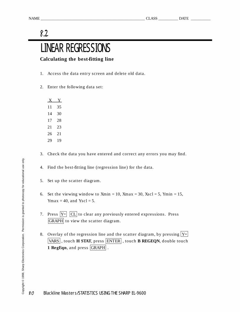
80 Blackline Masters/STATISTICS USING THE SHARP EL-9600Cop
yrig
ht ©
1998
, S
harp
Ele
ctro
nics
Cor
pora
tion.
Per
mis
sion
is g
rant
ed t
o ph
otoc
opy
for
educ
atio
nal u
se o
nly.
Calculating the best-fitting line
1. Access the data entry screen and delete old data.
2. Enter the following data set:
X Y
11 35
14 30
17 28
21 23
26 21
29 19
3. Check the data you have entered and correct any errors you may find.
4. Find the best-fitting line (regression line) for the data.
5. Set up the scatter diagram.
6. Set the viewing window to Xmin = 10, Xmax = 30, Xscl = 5, Ymin = 15,
Ymax = 40, and Yscl = 5.
7. Press Y= CL to clear any previously entered expressions. Press
GRAPH to view the scatter diagram.
8. Overlay of the regression line and the scatter diagram, by pressing Y=
VARS , touch H STAT, press ENTER , touch B REGEQN, double touch
1 RegEqn, and press GRAPH .
LINEAR REGRESSIONS 8.2
NAME _____________________________________________________ CLASS __________ DATE __________
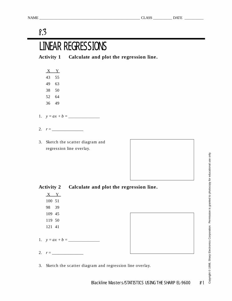
Blackline Masters/STATISTICS USING THE SHARP EL-9600 81 Cop
yrig
ht ©
1998
, S
harp
Ele
ctro
nics
Cor
pora
tion.
Per
mis
sion
is g
rant
ed t
o ph
otoc
opy
for
educ
atio
nal u
se o
nly.
Activity 1 Calculate and plot the regression line.
X Y
43 55
49 63
38 50
52 64
36 49
1. y = ax + b = _______________
2. r = _______________
3. Sketch the scatter diagram and
regression line overlay.
Activity 2 Calculate and plot the regression line. X Y
100 51
98 39
109 45
119 50
121 41
1. y = ax + b = _______________
2. r = _______________
3. Sketch the scatter diagram and regression line overlay.
LINEAR REGRESSIONS8.3
NAME _____________________________________________________ CLASS __________ DATE __________
82 Blackline Masters/STATISTICS USING THE SHARP EL-9600Cop
yrig
ht ©
1998
, S
harp
Ele
ctro
nics
Cor
pora
tion.
Per
mis
sion
is g
rant
ed t
o ph
otoc
opy
for
educ
atio
nal u
se o
nly.
Steps for calculating other regression models
1. Access the data entry screen and delete old data. Enter the following data set:
X Y
6 10
22 19
34 31
42 39
45 47
48 58
47 66
2. Check the data you have entered and correct any errors you may find.
3. Set up the scatter diagram.
4. Display the scatter diagram for the data by pressing WINDOW and
setting Xmin = 0, Xmax = 50, Xscl = 5, Ymin = 0, Ymax = 70, and Yscl = 5.
Press GRAPH to view the scatter diagram.
5. To find the best-fitting exponential curve (Y = a•ebX) for the data, press
STAT , touch D REG, touch on the screen, double touch 10 Rg_aebx,
and press ENTER .
6. To view the overlay of the regression curve and the scatter diagram, press
Y= CL VARS , touch H STAT, press ENTER , touch B REGEQN,
double touch 1 RegEqn, and press GRAPH .
7. Repeat this process to find and view other regression models.
OTHER REGRESSIONS9.1
NAME _____________________________________________________ CLASS __________ DATE __________
×+ –
÷
➧
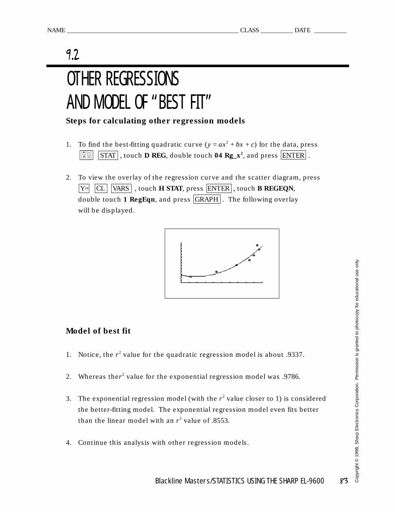
Blackline Masters/STATISTICS USING THE SHARP EL-9600 83 Cop
yrig
ht ©
1998
, S
harp
Ele
ctro
nics
Cor
pora
tion.
Per
mis
sion
is g
rant
ed t
o ph
otoc
opy
for
educ
atio
nal u
se o
nly.
Steps for calculating other regression models
1. To find the best-fitting quadratic curve (y = ax2 + bx + c) for the data, press
STAT , touch D REG, double touch 04 Rg_x2, and press ENTER .
2. To view the overlay of the regression curve and the scatter diagram, press
Y= CL VARS , touch H STAT, press ENTER , touch B REGEQN,
double touch 1 RegEqn, and press GRAPH . The following overlay
will be displayed.
Model of best fit
1. Notice, the r 2 value for the quadratic regression model is about .9337.
2. Whereas ther 2 value for the exponential regression model was .9786.
3. The exponential regression model (with the r 2 value closer to 1) is considered
the better-fitting model. The exponential regression model even fits better
than the linear model with an r 2 value of .8553.
4. Continue this analysis with other regression models.
OTHER REGRESSIONS AND MODEL OF “BEST FIT”
9.2
NAME _____________________________________________________ CLASS __________ DATE __________
×+ –
÷
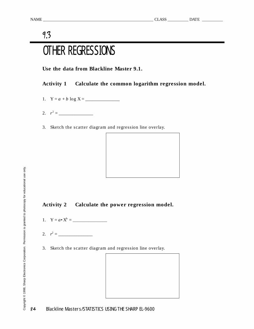
84 Blackline Masters/STATISTICS USING THE SHARP EL-9600Cop
yrig
ht ©
1998
, S
harp
Ele
ctro
nics
Cor
pora
tion.
Per
mis
sion
is g
rant
ed t
o ph
otoc
opy
for
educ
atio
nal u
se o
nly.
Use the data from Blackline Master 9.1.
Activity 1 Calculate the common logarithm regression model.
1. Y = a + b log X = _______________
2. r 2 = _______________
3. Sketch the scatter diagram and regression line overlay.
Activity 2 Calculate the power regression model.
1. Y = a•Xb = _______________
2. r2 = _______________
3. Sketch the scatter diagram and regression line overlay.
OTHER REGRESSIONS9.3
NAME _____________________________________________________ CLASS __________ DATE __________
Blackline Masters/STATISTICS USING THE SHARP EL-9600 85 Cop
yrig
ht ©
1998
, S
harp
Ele
ctro
nics
Cor
pora
tion.
Per
mis
sion
is g
rant
ed t
o ph
otoc
opy
for
educ
atio
nal u
se o
nly.
Use the data from Blackline Master 9.1.
Activity 3 Calculate the inverse regression model.
1. Y = a + bX-1 = _______________
2. r 2 = _______________
3. Sketch the scatter diagram and regression line overlay.
Activity 4 Which regression model fits the best?
1. r 2 for linear regression = _______________
2. r 2 for quadratic regression = _______________
3. r 2 for exponential regression = _______________
4. r 2 for common logarithm regression = _______________
5. r 2 for power regression = _______________
6. r 2 for inverse regression = _______________
7. Which model fits the best according to r 2? ____________
8. Which model fits the best graphically? _______________
OTHER REGRESSIONS AND MODEL OF “BEST FIT”
9.4
NAME _____________________________________________________ CLASS __________ DATE __________
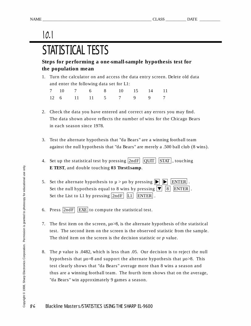
86 Blackline Masters/STATISTICS USING THE SHARP EL-9600Cop
yrig
ht ©
1998
, S
harp
Ele
ctro
nics
Cor
pora
tion.
Per
mis
sion
is g
rant
ed t
o ph
otoc
opy
for
educ
atio
nal u
se o
nly.
Steps for performing a one-small-sample hypothesis test for the population mean1. Turn the calculator on and access the data entry screen. Delete old data
and enter the following data set for L1:
7 10 7 6 8 10 15 14 11
12 6 11 11 5 7 9 9 7
2. Check the data you have entered and correct any errors you may find.
The data shown above reflects the number of wins for the Chicago Bears
in each season since 1978.
3. Test the alternate hypothesis that "da Bears" are a winning football team
against the null hypothesis that "da Bears" are merely a .500 ball club (8 wins).
4. Set up the statistical test by pressing 2ndF QUIT STAT , touching
E TEST, and double touching 03 Ttest1samp.
5. Set the alternate hypothesis to µ > µo by pressing ENTER .
Set the null hypothesis equal to 8 wins by pressing ▼ 8 ENTER .
Set the List to L1 by pressing 2ndF L1 ENTER .
6. Press 2ndF EXE to compute the statistical test.
7. The first item on the screen, µo>8, is the alternate hypothesis of the statistical
test. The second item on the screen is the observed statistic from the sample.
The third item on the screen is the decision statistic or p value.
8. The p value is .0482, which is less than .05. Our decision is to reject the null
hypothesis that µo=8 and support the alternate hypothesis that µo>8. This
test clearly shows that "da Bears" average more than 8 wins a season and
thus are a winning football team. The fourth item shows that on the average,
"da Bears" win approximately 9 games a season.
STATISTICAL TESTS10.1
NAME _____________________________________________________ CLASS __________ DATE __________
▼ ▼
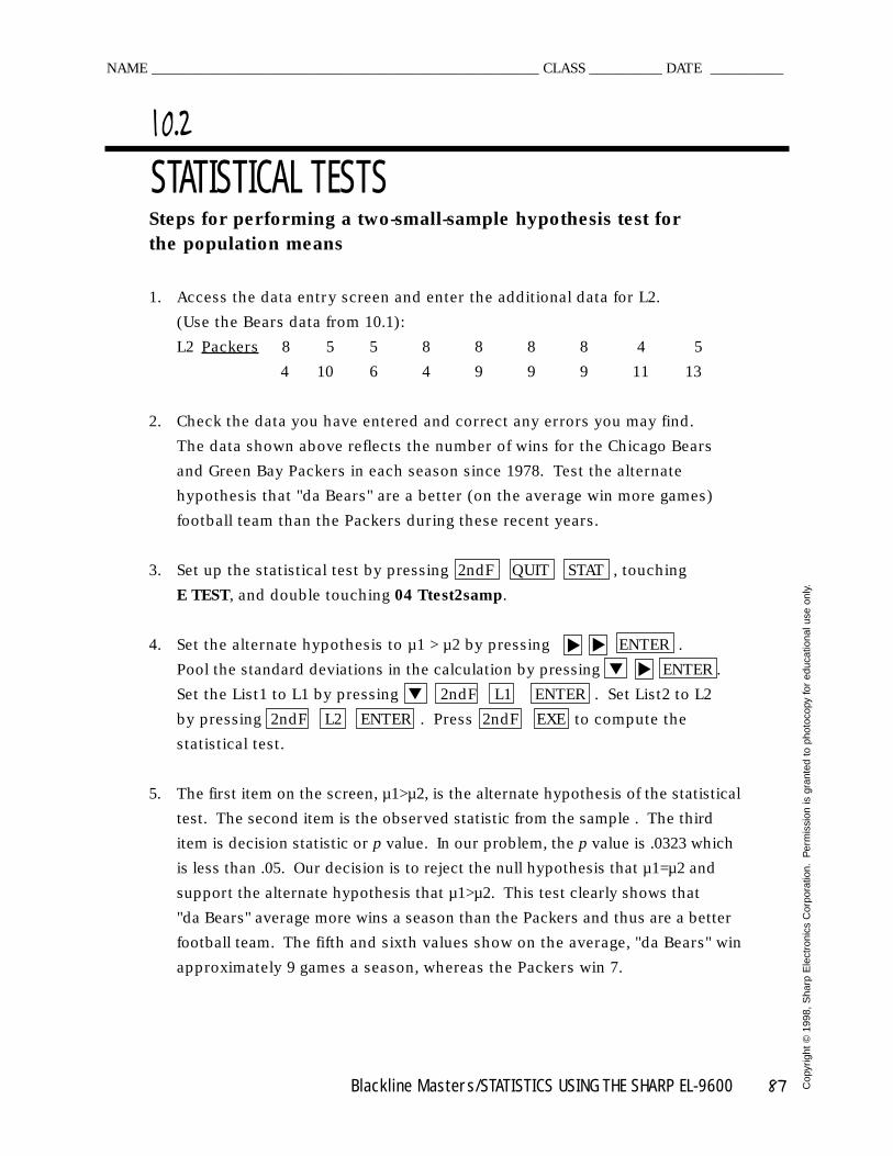
Blackline Masters/STATISTICS USING THE SHARP EL-9600 87 Cop
yrig
ht ©
1998
, S
harp
Ele
ctro
nics
Cor
pora
tion.
Per
mis
sion
is g
rant
ed t
o ph
otoc
opy
for
educ
atio
nal u
se o
nly.
Steps for performing a two-small-sample hypothesis test for the population means
1. Access the data entry screen and enter the additional data for L2.
(Use the Bears data from 10.1):
L2 Packers 8 5 5 8 8 8 8 4 5
4 10 6 4 9 9 9 11 13
2. Check the data you have entered and correct any errors you may find.
The data shown above reflects the number of wins for the Chicago Bears
and Green Bay Packers in each season since 1978. Test the alternate
hypothesis that "da Bears" are a better (on the average win more games)
football team than the Packers during these recent years.
3. Set up the statistical test by pressing 2ndF QUIT STAT , touching
E TEST, and double touching 04 Ttest2samp.
4. Set the alternate hypothesis to µ1 > µ2 by pressing ENTER .
Pool the standard deviations in the calculation by pressing ▼ ENTER .
Set the List1 to L1 by pressing ▼ 2ndF L1 ENTER . Set List2 to L2
by pressing 2ndF L2 ENTER . Press 2ndF EXE to compute the
statistical test.
5. The first item on the screen, µ1>µ2, is the alternate hypothesis of the statistical
test. The second item is the observed statistic from the sample . The third
item is decision statistic or p value. In our problem, the p value is .0323 which
is less than .05. Our decision is to reject the null hypothesis that µ1=µ2 and
support the alternate hypothesis that µ1>µ2. This test clearly shows that
"da Bears" average more wins a season than the Packers and thus are a better
football team. The fifth and sixth values show on the average, "da Bears" win
approximately 9 games a season, whereas the Packers win 7.
STATISTICAL TESTS10.2
NAME _____________________________________________________ CLASS __________ DATE __________
▼ ▼
▼
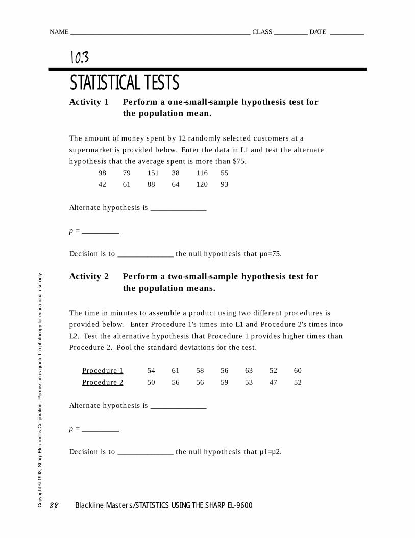
88 Blackline Masters/STATISTICS USING THE SHARP EL-9600Cop
yrig
ht ©
1998
, S
harp
Ele
ctro
nics
Cor
pora
tion.
Per
mis
sion
is g
rant
ed t
o ph
otoc
opy
for
educ
atio
nal u
se o
nly.
Activity 1 Perform a one-small-sample hypothesis test forthe population mean.
The amount of money spent by 12 randomly selected customers at a
supermarket is provided below. Enter the data in L1 and test the alternate
hypothesis that the average spent is more than $75.
98 79 151 38 116 55
42 61 88 64 120 93
Alternate hypothesis is _______________
p = __________
Decision is to _______________ the null hypothesis that µo=75.
Activity 2 Perform a two-small-sample hypothesis test forthe population means.
The time in minutes to assemble a product using two different procedures is
provided below. Enter Procedure 1's times into L1 and Procedure 2's times into
L2. Test the alternative hypothesis that Procedure 1 provides higher times than
Procedure 2. Pool the standard deviations for the test.
Procedure 1 54 61 58 56 63 52 60
Procedure 2 50 56 56 59 53 47 52
Alternate hypothesis is _______________
p = __________
Decision is to _______________ the null hypothesis that µ1=µ2.
STATISTICAL TESTS10.3
NAME _____________________________________________________ CLASS __________ DATE __________
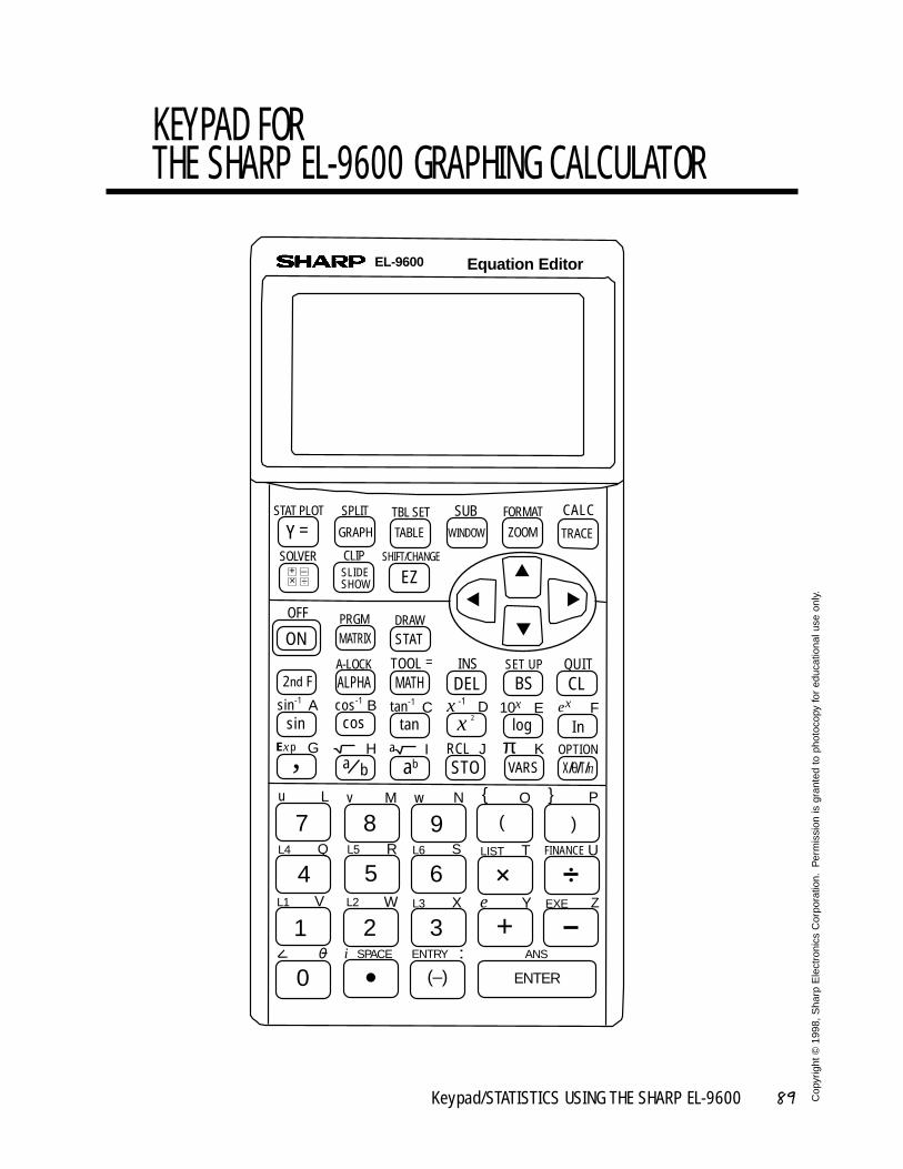
Keypad/STATISTICS USING THE SHARP EL-9600 89 Cop
yrig
ht ©
1998
, S
harp
Ele
ctro
nics
Cor
pora
tion.
Per
mis
sion
is g
rant
ed t
o ph
otoc
opy
for
educ
atio
nal u
se o
nly.
KEYPAD FOR THE SHARP EL-9600 GRAPHING CALCULATOR
CALCFORMATTBL SETSPLIT
CLIP
PRGM DRAW
INS
RCL
SET UP
OPTION
exx -1 10x F
P
)
}O
(
{N
9wM
8vL
7u
Q
4L4 R
5L5 S
6
+
+L6
X
:3
(–)
W
2L3L2V
1L1
O
0<
TLIST
SPACE ENTRY ANS
ENTER
Ye
i
ZEXE
UFINANCE
E
K
D
J π
C
QUIT
Inlog
VARS X/θ/T/n
tan
ab
tan-1
a
Bcos
cos-1
H Ia b
Asin
sin-1
G,Exp
x 2
A-LOCK TOOL =STAT
ALPHA MATH2nd F
MATRIX
OFF
ON
STAT PLOT
SOLVER
Y =
DEL
STO
BS CL
EZ
GRAPH TABLE
SUBTRACEZOOMWINDOW
SHIFT/CHANGESLIDESHOW×
+ –÷
▼
▼
▼
▼
Equation EditorEL-9600
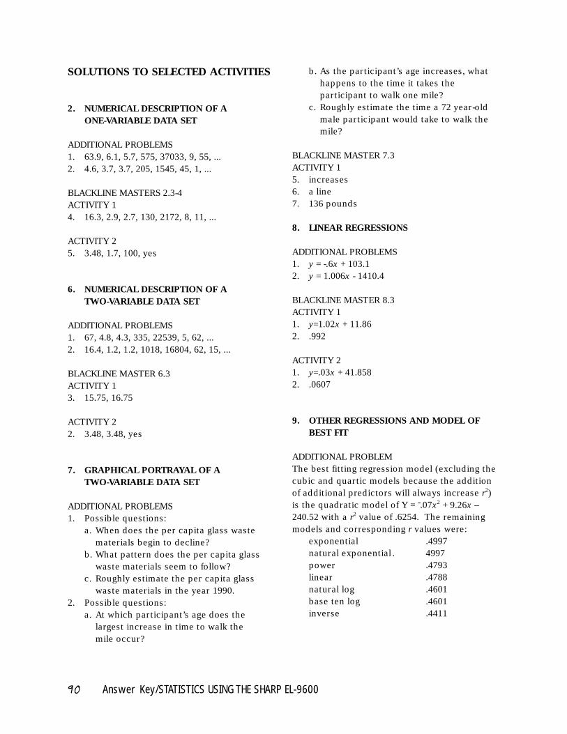
90 Answer Key/STATISTICS USING THE SHARP EL-9600
SOLUTIONS TO SELECTED ACTIVITIES
2. NUMERICAL DESCRIPTION OF A ONE-VARIABLE DATA SET
ADDITIONAL PROBLEMS1. 63.9, 6.1, 5.7, 575, 37033, 9, 55, ...2. 4.6, 3.7, 3.7, 205, 1545, 45, 1, ...
BLACKLINE MASTERS 2.3-4ACTIVITY 14. 16.3, 2.9, 2.7, 130, 2172, 8, 11, ...
ACTIVITY 25. 3.48, 1.7, 100, yes
6. NUMERICAL DESCRIPTION OF A TWO-VARIABLE DATA SET
ADDITIONAL PROBLEMS1. 67, 4.8, 4.3, 335, 22539, 5, 62, ...2. 16.4, 1.2, 1.2, 1018, 16804, 62, 15, ...
BLACKLINE MASTER 6.3ACTIVITY 13. 15.75, 16.75
ACTIVITY 22. 3.48, 3.48, yes
7. GRAPHICAL PORTRAYAL OF A TWO-VARIABLE DATA SET
ADDITIONAL PROBLEMS1. Possible questions:
a. When does the per capita glass waste materials begin to decline?
b. What pattern does the per capita glass waste materials seem to follow?
c. Roughly estimate the per capita glass waste materials in the year 1990.
2. Possible questions:a. At which participant’s age does the
largest increase in time to walk the mile occur?
b. As the participant’s age increases, what happens to the time it takes the participant to walk one mile?
c. Roughly estimate the time a 72 year-old male participant would take to walk the mile?
BLACKLINE MASTER 7.3ACTIVITY 15. increases6. a line7. 136 pounds
8. LINEAR REGRESSIONS
ADDITIONAL PROBLEMS1. y = -.6x + 103.12. y = 1.006x - 1410.4
BLACKLINE MASTER 8.3ACTIVITY 11. y=1.02x + 11.862. .992
ACTIVITY 21. y=.03x + 41.8582. .0607
9. OTHER REGRESSIONS AND MODEL OF BEST FIT
ADDITIONAL PROBLEMThe best fitting regression model (excluding the cubic and quartic models because the additionof additional predictors will always increase r2)is the quadratic model of Y = -.07x2 + 9.26x –240.52 with a r2 value of .6254. The remainingmodels and corresponding r values were:
exponential .4997natural exponential . 4997power .4793linear .4788natural log .4601base ten log .4601inverse .4411
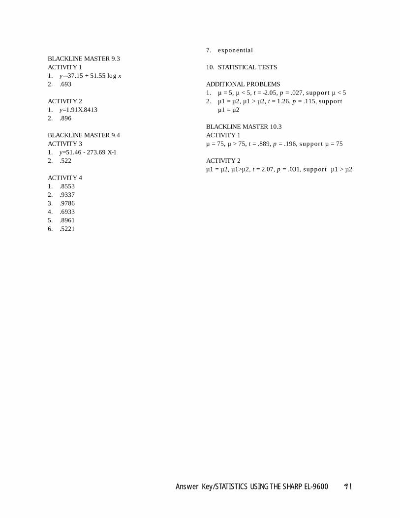
Answer Key/STATISTICS USING THE SHARP EL-9600 91
BLACKLINE MASTER 9.3ACTIVITY 11. y=-37.15 + 51.55 log x2. .693
ACTIVITY 21. y=1.91X.84132. .896
BLACKLINE MASTER 9.4ACTIVITY 31. y=51.46 - 273.69 X-12. .522
ACTIVITY 41. .85532. .93373. .97864. .69335. .89616. .5221
7. exponential
10. STATISTICAL TESTS
ADDITIONAL PROBLEMS1. µ = 5, µ < 5, t = -2.05, p = .027, support µ < 52. µ1 = µ2, µ1 > µ2, t = 1.26, p = .115, support
µ1 = µ2
BLACKLINE MASTER 10.3ACTIVITY 1µ = 75, µ > 75, t = .889, p = .196, support µ = 75
ACTIVITY 2µ1 = µ2, µ1>µ2, t = 2.07, p = .031, support µ1 > µ2

TEACHING NOTES
92 Teaching Notes/STATISTICS USING THE SHARP EL-9600

SHARP STAT COVER 02.2.19 11:09 AM Page 2