graphlab: a distributed abstraction for large...
TRANSCRIPT
GraphLab: A Distributed Abstraction for Large Scale Machine Learning
Yucheng Low
June 2013CMU-ML-13-104


GraphLab: A Distributed Abstractionfor Large Scale Machine Learning
Yucheng Low
June 2013CMU-ML-13-104
Machine Learning DepartmentSchool of Computer ScienceCarnegie Mellon University
Pittsburgh, PA 15213
Thesis Committee:Carlos Guestrin (Chair)
Guy E. BlellochDavid Andersen
Andrew Y. Ng (Stanford University)Joseph M. Hellerstein (University of California, Berkeley)
Submitted in partial fulfillment of the requirementsfor the degree of Doctor of Philosophy.
Copyright c© 2013 Yucheng Low
This research was sponsored by the Army Research Office under grant number W911NF0710287, the Office of Naval Researchunder grant numbers N000140710747, N000140810752, N000141010672, the National Science Foundation under grant numbersCNS0721591, IIS0803333, the Air Force Research Laboratory under grant number FA87500910141, and a fellowship from theIntel Science and Technology Center for Cloud Computing.
Abstract
Machine Learning methods have found increasing applicability and relevance to the realworld, finding applications in a broad range of fields in robotics, data mining, physics andbiology, among many others. However, with the growth of the World Wide Web, and withimprovements in data collection technology, real world datasets have been rapidly increasingin size and complexity, necessitating comparable scaling of Machine Learning algorithms.
However, designing and implementing efficient parallel Machine Learning algorithmsis challenging. Existing high-level parallel abstractions like MapReduce are insufficientlyexpressive while low-level tools such as MPI are difficult to use, and leave Machine Learningexperts repeatedly solving the same design challenges.
In this thesis, we trace the development of a framework called GraphLab which aims toprovide an expressive and efficient high level abstraction to satisfy the needs of a broad rangeof Machine Learning algorithms. We discuss the initial GraphLab design, including detailsof a shared memory and distributed memory implementation. Next, we discuss the scalinglimitations of GraphLab on real-world power-law graphs and how that informed the designof PowerGraph. By placing restrictions on the abstraction, we are able to improve scalability,demonstrating state of the art performance on a variety of benchmarks. Finally, we end withthe WarpGraph abstraction which improves usability of PowerGraph by combining featuresof GraphLab and PowerGraph to achieve an abstraction that is easy to use, scalable, and fast.
We demonstrate in this thesis, that by designing a domain specific abstraction for MachineLearning, we are able to provide a system that is both easy to use, and provides exceptionalscaling and performance on real world datasets.
Acknowledgments
I would like to thank my advisor, Carlos Guestrin, who provided crucial research guid-ance, without which this thesis would not have been possible. Carlos’s constant emphasisand guidance on the importance of writing and presentation skills has been invaluable to mydevelopment as a better communicator. Carlos had also put together a wonderful researchgroup of talented people who I would like to thank for their friendship and collaboration.
I began working with Joseph Gonzalez right from the beginning of graduate school andnearly all of my papers are coauthored with him. I thank Joseph for his continuous encour-agement and perseverance during difficult times. Our frequent discussions were crucial inthe formation of this thesis, and his development skills were essential to bring GraphLab tofruition. I also thank Joseph for his patience; his seek for perfection in writing quality, andhis truly amazing ability with PowerPoint animations.
The GraphLab project was developed by a small team consisting of Joseph Gonzalez,Danny Bickson, Aapo Kyrola and Haijie Gu. I collaborated with Joseph for the entirety ofthe GraphLab project and he has helped shape, develop and implement all versions of theabstraction. Danny Bickson has been instrumental emphasizing the importance of the sparsematrix factorization task and built the open source community around GraphLab. Aapo tooka different view of the abstraction, challenging the in-memory requirement of GraphLab,and built GraphChi, demonstrating that high performance computation on disk can be a real-ity. Haijie developed the graph partitioning heuristics in PowerGraph, which was pivotal forPowerGraph’s performance and success. Additionally, I would also like to thank Alex Smola,Joseph Hellerstein, Seth Goldstein and Guy Blelloch for their advice throughout the processof the GraphLab project.
I would also like to thank the Machine Learning Department at Carnegie Mellon Univer-sity which fostered a wonderful, friendly, collaborative environment for research.
Finally, I would like to thank all family and friends for their support.
Contents
1 Introduction 11.1 Design Goals . . . . . . . . . . . . . . . . . . . . . . . . . . . . . . . . . . . . . . . . . 2
1.1.1 Common Properties . . . . . . . . . . . . . . . . . . . . . . . . . . . . . . . . . 21.2 Thesis Statement . . . . . . . . . . . . . . . . . . . . . . . . . . . . . . . . . . . . . . . 31.3 Notation . . . . . . . . . . . . . . . . . . . . . . . . . . . . . . . . . . . . . . . . . . . . 3
2 GraphLab 1Graph As Computation 52.1 Graph-Parallel Abstractions . . . . . . . . . . . . . . . . . . . . . . . . . . . . . . . . . . 52.2 GraphLab Abstraction . . . . . . . . . . . . . . . . . . . . . . . . . . . . . . . . . . . . 7
2.2.1 Data Graph . . . . . . . . . . . . . . . . . . . . . . . . . . . . . . . . . . . . . . 72.2.2 Update Functions . . . . . . . . . . . . . . . . . . . . . . . . . . . . . . . . . . . 72.2.3 The GraphLab Execution Model . . . . . . . . . . . . . . . . . . . . . . . . . . . 82.2.4 Ensuring Serializability . . . . . . . . . . . . . . . . . . . . . . . . . . . . . . . . 92.2.5 Sync Operation and Global Values . . . . . . . . . . . . . . . . . . . . . . . . . . 92.2.6 Abstraction Summary . . . . . . . . . . . . . . . . . . . . . . . . . . . . . . . . 10
2.3 Shared Memory Implementation . . . . . . . . . . . . . . . . . . . . . . . . . . . . . . . 112.3.1 Engine . . . . . . . . . . . . . . . . . . . . . . . . . . . . . . . . . . . . . . . . 112.3.2 Schedulers . . . . . . . . . . . . . . . . . . . . . . . . . . . . . . . . . . . . . . 112.3.3 Evaluation . . . . . . . . . . . . . . . . . . . . . . . . . . . . . . . . . . . . . . 13
2.4 Distributed Implementation . . . . . . . . . . . . . . . . . . . . . . . . . . . . . . . . . . 222.4.1 The Data Graph . . . . . . . . . . . . . . . . . . . . . . . . . . . . . . . . . . . . 222.4.2 Engines . . . . . . . . . . . . . . . . . . . . . . . . . . . . . . . . . . . . . . . . 242.4.3 Fault Tolerance . . . . . . . . . . . . . . . . . . . . . . . . . . . . . . . . . . . . 262.4.4 Evaluation . . . . . . . . . . . . . . . . . . . . . . . . . . . . . . . . . . . . . . 28
2.5 Conclusion . . . . . . . . . . . . . . . . . . . . . . . . . . . . . . . . . . . . . . . . . . 34
3 PowerGraphRestricting the Abstraction for Performance 353.1 GraphLab 1 Limitations . . . . . . . . . . . . . . . . . . . . . . . . . . . . . . . . . . . . 35
3.1.1 Gather vs Scatter . . . . . . . . . . . . . . . . . . . . . . . . . . . . . . . . . . . 363.1.2 Natural Graphs . . . . . . . . . . . . . . . . . . . . . . . . . . . . . . . . . . . . 363.1.3 Serializability Frequently Unnecessary . . . . . . . . . . . . . . . . . . . . . . . 39
3.2 Characterization . . . . . . . . . . . . . . . . . . . . . . . . . . . . . . . . . . . . . . . . 393.3 PowerGraph Abstraction . . . . . . . . . . . . . . . . . . . . . . . . . . . . . . . . . . . 40
3.3.1 GAS Vertex-Programs . . . . . . . . . . . . . . . . . . . . . . . . . . . . . . . . 41
iv
3.3.2 Delta Caching . . . . . . . . . . . . . . . . . . . . . . . . . . . . . . . . . . . . . 433.3.3 Scheduling . . . . . . . . . . . . . . . . . . . . . . . . . . . . . . . . . . . . . . 433.3.4 Comparison with GraphLab 1 and Pregel . . . . . . . . . . . . . . . . . . . . . . 45
3.4 Distributed Graph Placement . . . . . . . . . . . . . . . . . . . . . . . . . . . . . . . . . 453.4.1 Balanced p-way Vertex-Cut . . . . . . . . . . . . . . . . . . . . . . . . . . . . . 473.4.2 Greedy Vertex-Cuts . . . . . . . . . . . . . . . . . . . . . . . . . . . . . . . . . . 49
3.5 Abstraction Comparison . . . . . . . . . . . . . . . . . . . . . . . . . . . . . . . . . . . 513.5.1 Computation Imbalance . . . . . . . . . . . . . . . . . . . . . . . . . . . . . . . 523.5.2 Communication Imbalance . . . . . . . . . . . . . . . . . . . . . . . . . . . . . . 533.5.3 Runtime Comparison . . . . . . . . . . . . . . . . . . . . . . . . . . . . . . . . . 53
3.6 Implementation and Evaluation . . . . . . . . . . . . . . . . . . . . . . . . . . . . . . . . 543.6.1 Graph Loading and Placement . . . . . . . . . . . . . . . . . . . . . . . . . . . . 543.6.2 Synchronous Engine (Sync) . . . . . . . . . . . . . . . . . . . . . . . . . . . . . 543.6.3 Asynchronous Engine (Async) . . . . . . . . . . . . . . . . . . . . . . . . . . . . 563.6.4 Async. Serializable Engine (Async+S) . . . . . . . . . . . . . . . . . . . . . . . 563.6.5 Fault Tolerance . . . . . . . . . . . . . . . . . . . . . . . . . . . . . . . . . . . . 583.6.6 Applications . . . . . . . . . . . . . . . . . . . . . . . . . . . . . . . . . . . . . 58
3.7 Conclusion . . . . . . . . . . . . . . . . . . . . . . . . . . . . . . . . . . . . . . . . . . 59
4 WarpGraphFine Grained Data-Parallelism for Usability 614.1 PowerGraph Limitations . . . . . . . . . . . . . . . . . . . . . . . . . . . . . . . . . . . 61
4.1.1 Expressiveness . . . . . . . . . . . . . . . . . . . . . . . . . . . . . . . . . . . . 624.1.2 Usability . . . . . . . . . . . . . . . . . . . . . . . . . . . . . . . . . . . . . . . 62
4.2 WarpGraph . . . . . . . . . . . . . . . . . . . . . . . . . . . . . . . . . . . . . . . . . . 654.2.1 Update Function . . . . . . . . . . . . . . . . . . . . . . . . . . . . . . . . . . . 654.2.2 Fine Grained Data-Parallel Primitives . . . . . . . . . . . . . . . . . . . . . . . . 664.2.3 Expressiveness . . . . . . . . . . . . . . . . . . . . . . . . . . . . . . . . . . . . 69
4.3 Implementation . . . . . . . . . . . . . . . . . . . . . . . . . . . . . . . . . . . . . . . . 704.4 Evaluation . . . . . . . . . . . . . . . . . . . . . . . . . . . . . . . . . . . . . . . . . . . 72
4.4.1 PageRank . . . . . . . . . . . . . . . . . . . . . . . . . . . . . . . . . . . . . . . 724.4.2 Graph Coloring . . . . . . . . . . . . . . . . . . . . . . . . . . . . . . . . . . . . 734.4.3 Stochastic Gradient Descent . . . . . . . . . . . . . . . . . . . . . . . . . . . . . 74
4.5 Conclusion . . . . . . . . . . . . . . . . . . . . . . . . . . . . . . . . . . . . . . . . . . 77
5 Related Work 795.1 Map-Reduce Abstraction . . . . . . . . . . . . . . . . . . . . . . . . . . . . . . . . . . 79
5.1.1 Relation to GraphLab . . . . . . . . . . . . . . . . . . . . . . . . . . . . . . . . . 805.2 BSP Abstraction (Pregel) . . . . . . . . . . . . . . . . . . . . . . . . . . . . . . . . . . . 80
5.2.1 Dynamic Execution . . . . . . . . . . . . . . . . . . . . . . . . . . . . . . . . . . 815.2.2 Asynchronous Computation . . . . . . . . . . . . . . . . . . . . . . . . . . . . . 815.2.3 Edge Data . . . . . . . . . . . . . . . . . . . . . . . . . . . . . . . . . . . . . . . 815.2.4 Generalized Messaging . . . . . . . . . . . . . . . . . . . . . . . . . . . . . . . . 825.2.5 Scatter vs Gather . . . . . . . . . . . . . . . . . . . . . . . . . . . . . . . . . . . 825.2.6 Relation to GraphLab . . . . . . . . . . . . . . . . . . . . . . . . . . . . . . . . . 83
5.3 Generalized SpMV Abstraction . . . . . . . . . . . . . . . . . . . . . . . . . . . . . . . . 835.3.1 Relation to GraphLab . . . . . . . . . . . . . . . . . . . . . . . . . . . . . . . . . 83
v
5.4 Dataflow Abstraction . . . . . . . . . . . . . . . . . . . . . . . . . . . . . . . . . . . . . 835.4.1 Relation to GraphLab . . . . . . . . . . . . . . . . . . . . . . . . . . . . . . . . . 84
5.5 Datalog/Bloom . . . . . . . . . . . . . . . . . . . . . . . . . . . . . . . . . . . . . . . . 84
6 Conclusion 856.1 Thesis Summary . . . . . . . . . . . . . . . . . . . . . . . . . . . . . . . . . . . . . . . 856.2 Observations . . . . . . . . . . . . . . . . . . . . . . . . . . . . . . . . . . . . . . . . . 866.3 Future Work . . . . . . . . . . . . . . . . . . . . . . . . . . . . . . . . . . . . . . . . . . 89
6.3.1 Graph Partitioning . . . . . . . . . . . . . . . . . . . . . . . . . . . . . . . . . . 896.3.2 Incremental Machine Learning . . . . . . . . . . . . . . . . . . . . . . . . . . . . 896.3.3 Dynamic Execution . . . . . . . . . . . . . . . . . . . . . . . . . . . . . . . . . . 896.3.4 Fault Tolerance . . . . . . . . . . . . . . . . . . . . . . . . . . . . . . . . . . . . 906.3.5 Other Abstractions . . . . . . . . . . . . . . . . . . . . . . . . . . . . . . . . . . 906.3.6 Parameter Server . . . . . . . . . . . . . . . . . . . . . . . . . . . . . . . . . . . 91
A Extended Chandy Misra 92A.1 Chandy Misra . . . . . . . . . . . . . . . . . . . . . . . . . . . . . . . . . . . . . . . . . 92A.2 Hierarchical Chandy Misra . . . . . . . . . . . . . . . . . . . . . . . . . . . . . . . . . . 93
B Algorithm Examples 96B.1 PageRank . . . . . . . . . . . . . . . . . . . . . . . . . . . . . . . . . . . . . . . . . . . 96B.2 Connected Component . . . . . . . . . . . . . . . . . . . . . . . . . . . . . . . . . . . . 98B.3 Triangle Counting . . . . . . . . . . . . . . . . . . . . . . . . . . . . . . . . . . . . . . . 100B.4 Collaborative Filtering . . . . . . . . . . . . . . . . . . . . . . . . . . . . . . . . . . . . 102B.5 Belief Propagation . . . . . . . . . . . . . . . . . . . . . . . . . . . . . . . . . . . . . . 106
C Dataset List 110
Bibliography 111
vi
Chapter 1
Introduction
The field of Machine Learning (ML) has matured significantly in the last few decades, making it in-creasingly relevant to the real world. Simultaneously, with the growth of the World Wide Web and withimprovements in data collection capabilities, real world dataset sizes have been experiencing exponen-tial growth rates; growing beyond the capability of what most research groups can handle. For instance:Facebook now reaches to over 845 million users: increasing by 237 million in the last year1; Youtube nowobserves an average of 48 hours of video uploaded per minute, increasing by a factor of two over the lastyear2. While simple ML methods which only require moments of the data [Chu et al., 2007] can copewith such large datasets with ease, in many cases more sophisticated algorithms can provide increasedaccuracy and performance. However, such advanced algorithms are also significantly harder to implementand scale. To increase applicability of ML methods to the real world, there is a need for scalable systemsthat can execute modern ML algorithms on large dataset sizes.
Unfortunately, existing high level parallel abstractions such as MapReduce [Dean and Ghemawat, 2004],Dryad [Isard et al., 2007], Pregel [Malewicz et al., 2010] among others, do not provide sufficient ex-pressiveness for large classes of Machine Learning algorithms, requiring excessive programmer effort,or incurring unnecessary inefficiency and overhead. Alternatively, implementing ML algorithms on lowlevel frameworks such as OpenMP [Dagum and Menon, 1998] or MPI [Gropp et al., 1996] can be chal-lenging, requiring the user to address complex issues like race conditions, deadlocks, communication andsynchronization.
In this thesis, we propose a computation abstraction called GraphLab based on sparse graph structures, thatwe find to be widely applicable to a broad range of Machine Learning problems. We track the evolutionof the abstraction over the years (renaming it as PowerGraph, and WarpGraph) as we modify it to resolvescalability and usability issues. While the subsequent abstractions have different names, they revolvearound the same original GraphLab abstraction blueprint. The thesis is organized as follows:
Section 1.1: Design Goals Describe the computation needs of Machine Learning Algorithms, and howexisting computation abstractions fail to address these requirements.
Chapter 2: GraphLab 1 Our first attempt at a unified ML abstraction which addresses these computa-tion needs for the shared and distributed memory setting.
1http://www.facebook.com/press/info.php?timeline2http://youtube-global.blogspot.com/2011/05/thanks-youtube-community-for-two-big.html
1
Chapter 3: PowerGraph GraphLab was powerful and easy to use, but encounters severe scalability lim-itations with power-law graphs. PowerGraph introduces restrictions on the Graphlab 1 abstraction toimprove efficiency and scalability, achieving unparalleled performance on a variety of benchmarks.
Chapter 4: WarpGraph PowerGraph was fast, but difficult to use in practice due to its restrictions.WarpGraph, combines features of GraphLab 1 and PowerGraph to provide a new abstraction toprovide both the ease of use of GraphLab 1, and the performance of PowerGraph.
Chapter 5: Related Work We discuss the similarities and differences between the work in this thesisand other related abstractions.
Chapter 6: Conclusion We conclude and summarize the thesis. We discuss how GraphLab fits in thebigger picture of Large Scale Machine Learning and the future research directions that can follow.
Appendix A: Chandy Misra We describe a hierarchical extension to the Chandy-Misra algorithm [Chandyand Misra, 1984], which we used to provide distributed locking in PowerGraph.
Appendix B: Algorithm Examples We provide five algorithm examples implemented in all three ab-stractions.
Appendix C: Dataset List A list of all experimental datasets used for testing and benchmarking.
1.1 Design Goals
The goal of this thesis is to design, and implement a computation abstraction which is uniquely designed totarget the needs of many Machine Learning algorithms. To do so, it is necessary to understand the commonproperties that exist in many Machine Learning algorithms and how existing computation abstractions failto address these properties.
1.1.1 Common Properties
Interdependent Computation: Many of the recent advances in ML have focused on modeling the de-pendencies between data. By modeling data dependencies, we are able to extract more signal from noisydata and build a deeper understanding. For example, modeling the dependencies between similar shoppersin a semi-supervised or transductive learning setting allows us to make better product recommendationsthan treating shoppers in isolation. Unfortunately, data parallel abstractions like MapReduce [Dean andGhemawat, 2004] are not generally well suited for the dependent computation typically required by moreadvanced ML algorithms. Although it is often possible to transform algorithms with computational de-pendencies into MapReduce algorithms, the resulting transformations can introduce inefficiencies.
Asynchronous Iterative Computation: Many important machine learning algorithms iteratively updatelarge collections of parameters. Unlike synchronous computation, in which all parameters are updatedsimultaneously (in parallel) using the previous parameters values, asynchronous computation allows in-dividual parameter updates to use the most recently available values for dependent parameters. Asyn-chronous computation provides many ML algorithms with significant algorithmic benefits. For example,linear systems (common to many ML algorithms) have been theoretically shown in Bertsekas and Tsitsik-lis [1989] to converge faster when solved asynchronously. Additionally, there are numerous cases in MLwhere asynchronous procedures have been empirically shown to significantly outperform synchronous
2
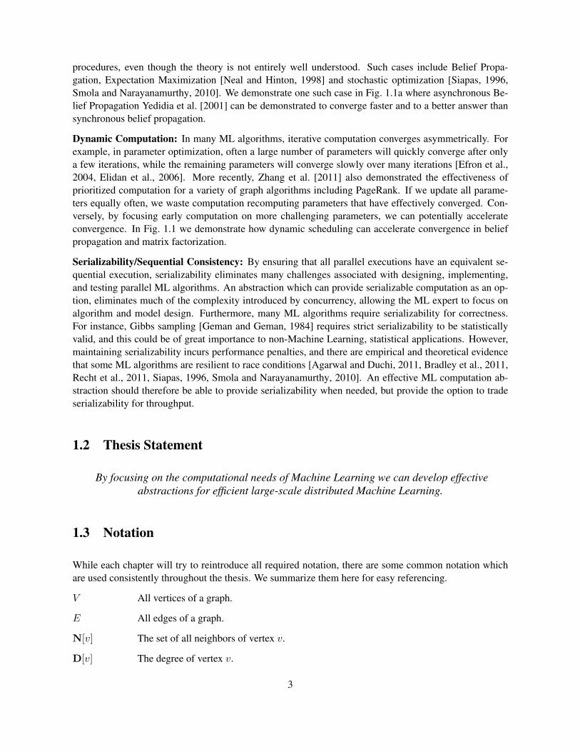
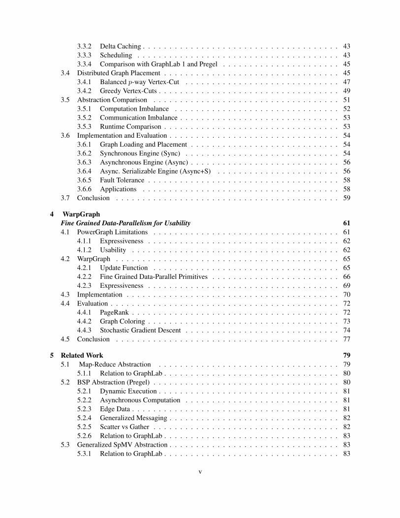
procedures, even though the theory is not entirely well understood. Such cases include Belief Propa-gation, Expectation Maximization [Neal and Hinton, 1998] and stochastic optimization [Siapas, 1996,Smola and Narayanamurthy, 2010]. We demonstrate one such case in Fig. 1.1a where asynchronous Be-lief Propagation Yedidia et al. [2001] can be demonstrated to converge faster and to a better answer thansynchronous belief propagation.
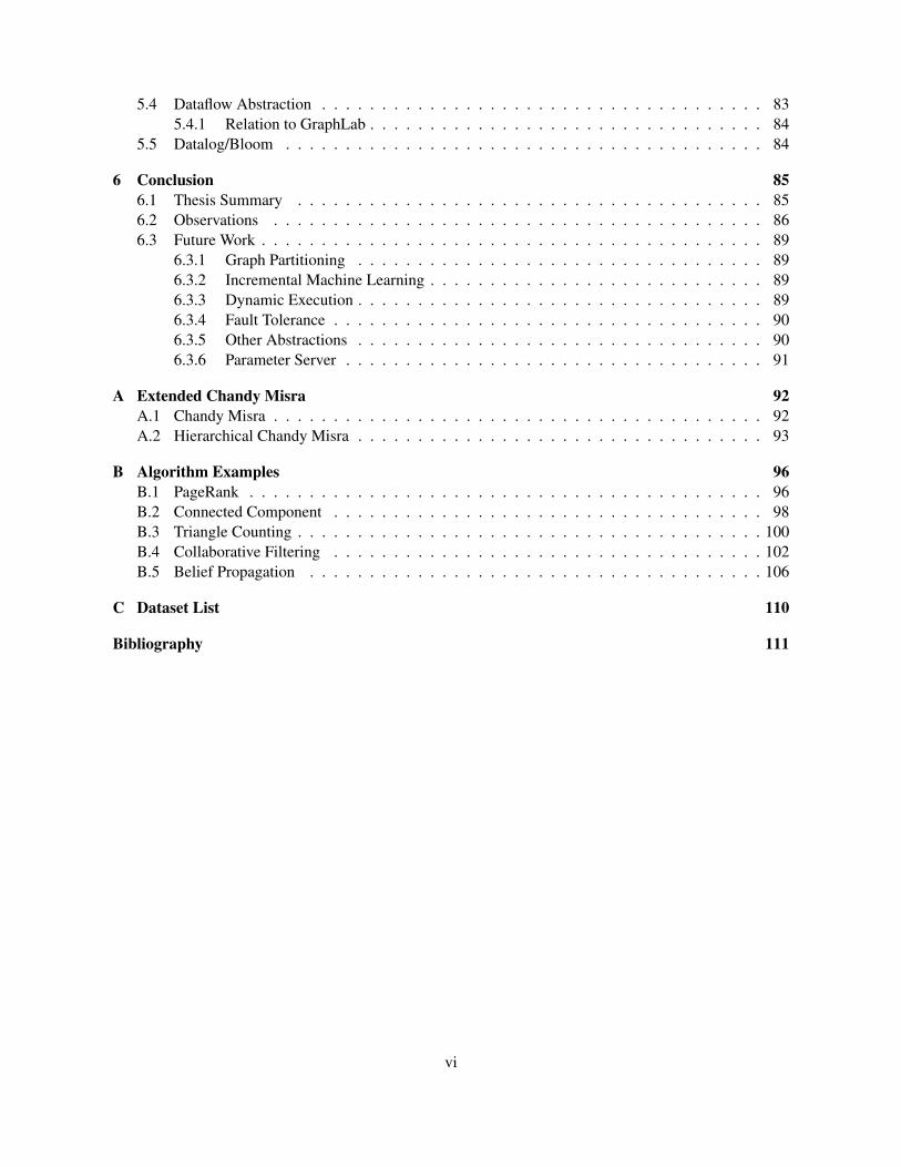
Dynamic Computation: In many ML algorithms, iterative computation converges asymmetrically. Forexample, in parameter optimization, often a large number of parameters will quickly converge after onlya few iterations, while the remaining parameters will converge slowly over many iterations [Efron et al.,2004, Elidan et al., 2006]. More recently, Zhang et al. [2011] also demonstrated the effectiveness ofprioritized computation for a variety of graph algorithms including PageRank. If we update all parame-ters equally often, we waste computation recomputing parameters that have effectively converged. Con-versely, by focusing early computation on more challenging parameters, we can potentially accelerateconvergence. In Fig. 1.1 we demonstrate how dynamic scheduling can accelerate convergence in beliefpropagation and matrix factorization.
Serializability/Sequential Consistency: By ensuring that all parallel executions have an equivalent se-quential execution, serializability eliminates many challenges associated with designing, implementing,and testing parallel ML algorithms. An abstraction which can provide serializable computation as an op-tion, eliminates much of the complexity introduced by concurrency, allowing the ML expert to focus onalgorithm and model design. Furthermore, many ML algorithms require serializability for correctness.For instance, Gibbs sampling [Geman and Geman, 1984] requires strict serializability to be statisticallyvalid, and this could be of great importance to non-Machine Learning, statistical applications. However,maintaining serializability incurs performance penalties, and there are empirical and theoretical evidencethat some ML algorithms are resilient to race conditions [Agarwal and Duchi, 2011, Bradley et al., 2011,Recht et al., 2011, Siapas, 1996, Smola and Narayanamurthy, 2010]. An effective ML computation ab-straction should therefore be able to provide serializability when needed, but provide the option to tradeserializability for throughput.
1.2 Thesis Statement
By focusing on the computational needs of Machine Learning we can develop effectiveabstractions for efficient large-scale distributed Machine Learning.
1.3 Notation
While each chapter will try to reintroduce all required notation, there are some common notation whichare used consistently throughout the thesis. We summarize them here for easy referencing.
V All vertices of a graph.
E All edges of a graph.
N[v] The set of all neighbors of vertex v.
D[v] The degree of vertex v.
3
0 5 10 15 20
10−6
10−4
10−2
Sweeps
Res
idua
l
BSP
Asynchronous
Dynamic Asynchronous
(a) LoopyBP
0.5 1 1.5 2 2.5
x 106
1
1.2
1.4
1.6
1.8
2
2.2
Number of updates
RM
SE
Round−robin
τ = 5
τ = 10
(b) Matrix Factorization
Figure 1.1: (a) To compare the efficiency of different computation models we plot the level of convergence ofBelief Propagation as a function of time using synchronous (BSP), asynchronous and dynamic schedulings. Thedifference in convergence is discussed in Gonzalez et al. [2009b]. (b) Convergence speed of Matrix factorizationusing Alternative Least Squares comparing full round-robin updates and using dynamic scheduling with differentskipping thresholds (τ ). Skipping updates on relatively converged vertices leads to focused computation and asconsequence, faster convergence.
Dv The data stored on a vertex v.
Du→v The data stored on the directed edge u→ v.
Du−v Refer to either the data located on u→ v or v → u depending on context (See Sec. 2.2.1).
D∗→v The set of all data on in-vertices to vertex v. Formally, {Du : (u→ v) ∈ E}
Dv→∗ The set of all data on out-vertices to vertex v. Formally, {Du : (v → u) ∈ E}
D The set of all data on all edges and vertices of the graph.
4
Chapter 2
GraphLab 1
Graph As Computation
In this chapter, we begin by defining the first version of the GraphLab abstraction in Sec. 2.2 whichcomprises of
1. A data graph which represents the data and computational dependencies,
2. An update function which describe local computation on the graph,
3. Scheduling primitives which express the order of computation,
4. A data consistency model, which determines the extent to which computation can overlap,
5. And a Sync mechanism for aggregating global state.
Next, in Sec. 2.3, we describe an implementation of the GraphLab abstraction in the shared memorysetting [Low et al., 2010], and provide an extensive evaluation of the implementation on five MachineLearning tasks, demonstrating the expressiveness and performance of the GraphLab abstraction.
Finally, in Sec. 2.4 we extend the shared memory implementation to the distributed setting [Low et al.,2012], addressing the difficulties of state partitioning, data consistency, and fault tolerance. We evaluateour implementation on three Machine Learning tasks and show that we are able to achieve good distributedperformance.
2.1 Graph-Parallel Abstractions
Large-scale graph-structured computation is central to many recent advances in ML. From modeling thecoupled interests of friends in a social network to the topical relationship between connected documents,graphs encode dependencies in data. The data dependencies encoded by graphs often lead to computa-tional dependencies in ML algorithms. For example, to estimate the interests of individuals in a socialnetwork, an ML algorithm might iteratively optimize parameters for each individual conditioned on thecurrent best parameters for their friends.
5
Unfortunately, high-level data-parallel frameworks such as Map-Reduce [Dean and Ghemawat, 2004] arenot well suited for graph-structured computation. As a consequence some [Asuncion et al., 2009, Gonza-lez et al., 2009a, Graf et al., 2005, Nallapati et al., 2007, Newman et al., 2008, Smola and Narayanamurthy,2010] have adopted low-level tools and techniques to build large-scale distributed systems. This approachblends statistical models and algorithms with distributed system design leads to systems that are special-ized and difficult to extend. In ordered to avoid the challenges of distributed system design, others havetried to adapt their algorithms to high-level data-parallel abstractions such as MapReduce. However, thisapproach does not exploit the structure of the problem and can lead to inefficient systems.
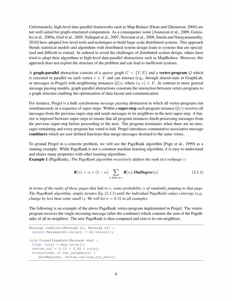
A graph-parallel abstraction consists of a sparse graph G = {V,E} and a vertex-program Q whichis executed in parallel on each vertex v ∈ V and can interact (e.g., through shared-state in GraphLab,or messages in Pregel) with neighboring instances Q(u) where (u, v) ∈ E. In contrast to more generalmessage passing models, graph-parallel abstractions constrain the interaction between vertex-programs toa graph structure enabling the optimization of data-layout and communication.
For instance, Pregel is a bulk synchronous message passing abstraction in which all vertex-programs runsimultaneously in a sequence of super-steps. Within a super-step each program instanceQ(v) receives allmessages from the previous super-step and sends messages to its neighbors in the next super-step. A bar-rier is imposed between super-steps to ensure that all program instances finish processing messages fromthe previous super-step before proceeding to the next. The program terminates when there are no mes-sages remaining and every program has voted to halt. Pregel introduces commutative associative messagecombiners which are user defined functions that merge messages destined to the same vertex.
To ground Pregel in a concrete problem, we will use the PageRank algorithm [Page et al., 1999] as arunning example. While PageRank is not a common machine learning algorithm, it is easy to understandand shares many properties with other learning algorithms.Example 1 (PageRank). The PageRank algorithm recursively defines the rank of a webpage v:
R(v) = α+ (1− α)∑
u links to v
R(u)/OutDegree(u) (2.1.1)
in terms of the ranks of those pages that link to v, some probability α of randomly jumping to that page.The PageRank algorithm, simply iterates Eq. (2.1.1) until the individual PageRank values converge (e.g.,change by less than some small ε). We will let α = 0.15 in all examples.
The following is an example of the above PageRank vertex-program implemented in Pregel. The vertex-program receives the single incoming message (after the combiner) which contains the sum of the PageR-anks of all in-neighbors. The new PageRank is then computed and sent to its out-neighbors.
Message combiner(Message m1, Message m2) :return Message(m1.value() + m2.value());
void PregelPageRank(Message msg) :float total = msg.value();vertex.val = 0.15 + 0.85 * total;foreach(nbr in out_neighbors) :
SendMsg(nbr, vertex.val/num_out_nbrs);
6
3
4
D11 2
5
D1↔2
D2↔3D1↔3
D1↔4
D3↔4 D3↔5
D4↔5
Scope S1
Vertex Data
Edge Data
Data Graph
D2
D5D4
D3
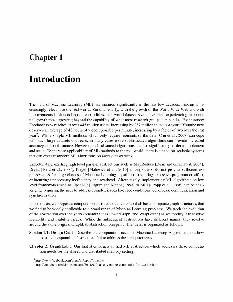
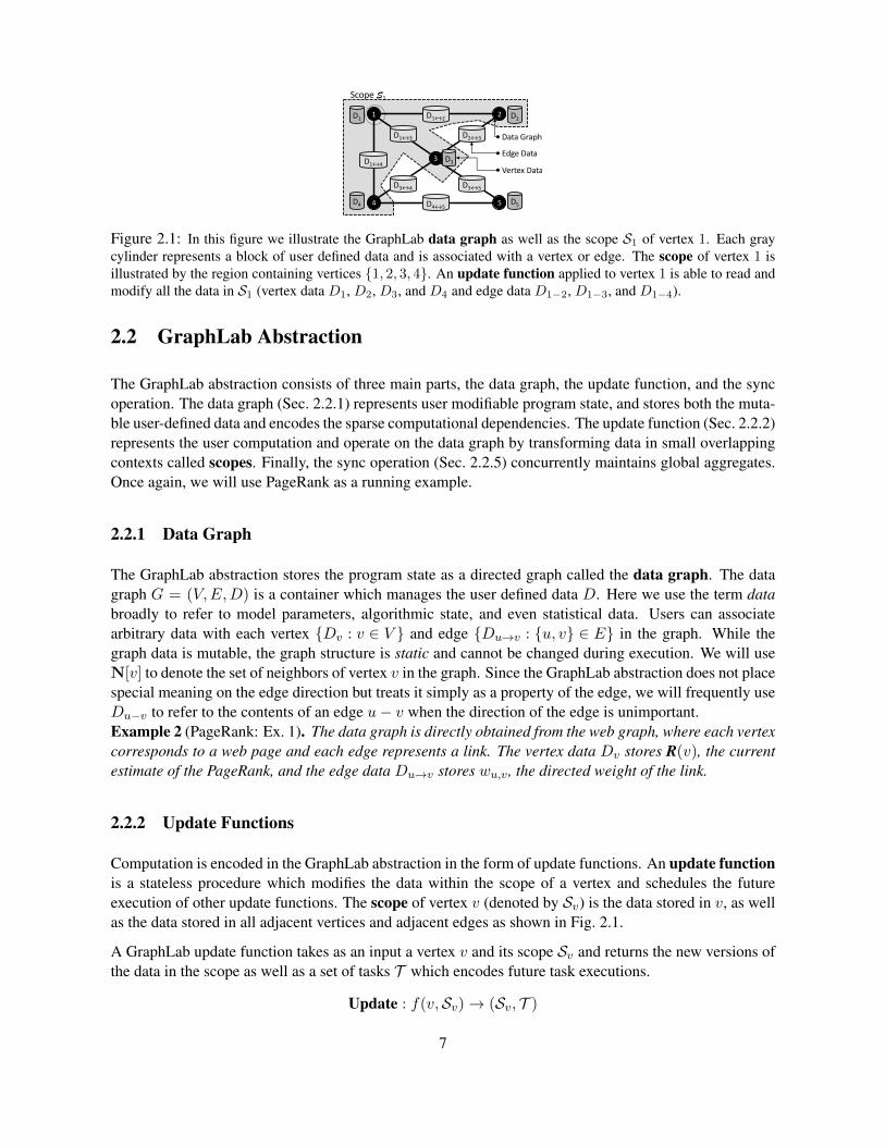
Figure 2.1: In this figure we illustrate the GraphLab data graph as well as the scope S1 of vertex 1. Each graycylinder represents a block of user defined data and is associated with a vertex or edge. The scope of vertex 1 isillustrated by the region containing vertices {1, 2, 3, 4}. An update function applied to vertex 1 is able to read andmodify all the data in S1 (vertex data D1, D2, D3, and D4 and edge data D1−2, D1−3, and D1−4).
2.2 GraphLab Abstraction
The GraphLab abstraction consists of three main parts, the data graph, the update function, and the syncoperation. The data graph (Sec. 2.2.1) represents user modifiable program state, and stores both the muta-ble user-defined data and encodes the sparse computational dependencies. The update function (Sec. 2.2.2)represents the user computation and operate on the data graph by transforming data in small overlappingcontexts called scopes. Finally, the sync operation (Sec. 2.2.5) concurrently maintains global aggregates.Once again, we will use PageRank as a running example.
2.2.1 Data Graph
The GraphLab abstraction stores the program state as a directed graph called the data graph. The datagraph G = (V,E,D) is a container which manages the user defined data D. Here we use the term databroadly to refer to model parameters, algorithmic state, and even statistical data. Users can associatearbitrary data with each vertex {Dv : v ∈ V } and edge {Du→v : {u, v} ∈ E} in the graph. While thegraph data is mutable, the graph structure is static and cannot be changed during execution. We will useN[v] to denote the set of neighbors of vertex v in the graph. Since the GraphLab abstraction does not placespecial meaning on the edge direction but treats it simply as a property of the edge, we will frequently useDu−v to refer to the contents of an edge u− v when the direction of the edge is unimportant.Example 2 (PageRank: Ex. 1). The data graph is directly obtained from the web graph, where each vertexcorresponds to a web page and each edge represents a link. The vertex data Dv stores R(v), the currentestimate of the PageRank, and the edge data Du→v stores wu,v, the directed weight of the link.
2.2.2 Update Functions
Computation is encoded in the GraphLab abstraction in the form of update functions. An update functionis a stateless procedure which modifies the data within the scope of a vertex and schedules the futureexecution of other update functions. The scope of vertex v (denoted by Sv) is the data stored in v, as wellas the data stored in all adjacent vertices and adjacent edges as shown in Fig. 2.1.
A GraphLab update function takes as an input a vertex v and its scope Sv and returns the new versions ofthe data in the scope as well as a set of tasks T which encodes future task executions.
Update : f(v,Sv)→ (Sv, T )
7
After executing an update function the modified scope data in Sv is written back to the data graph. Eachtask in the set of tasks T , is a tuple (f, v) consisting of an update function f and a vertex v. All re-turned tasks T are executed eventually by running f(v,Sv) following the execution semantics describedin Sec. 2.2.3.
Rather than adopting a message passing or data flow model as in Isard et al. [2007], Malewicz et al.[2010], GraphLab allows the user defined update functions complete freedom to read and modify any ofthe data on adjacent vertices and edges. This simplifies user code and eliminates the need for the users toreason about the movement of data. By controlling what tasks are added to the task set, GraphLab updatefunctions can efficiently express adaptive computation. For example, an update function may choose toreschedule its neighbors only when it has made a substantial change to its local data.Example 3 (PageRank: Ex. 1). The update function for PageRank (defined in Alg. 2.1) computes aweighted sum of the current ranks of neighboring vertices and assigns it as the rank of the current vertex.The algorithm is adaptive: neighbors are listed for update only if the value of current vertex changes morethan a predefined threshold.
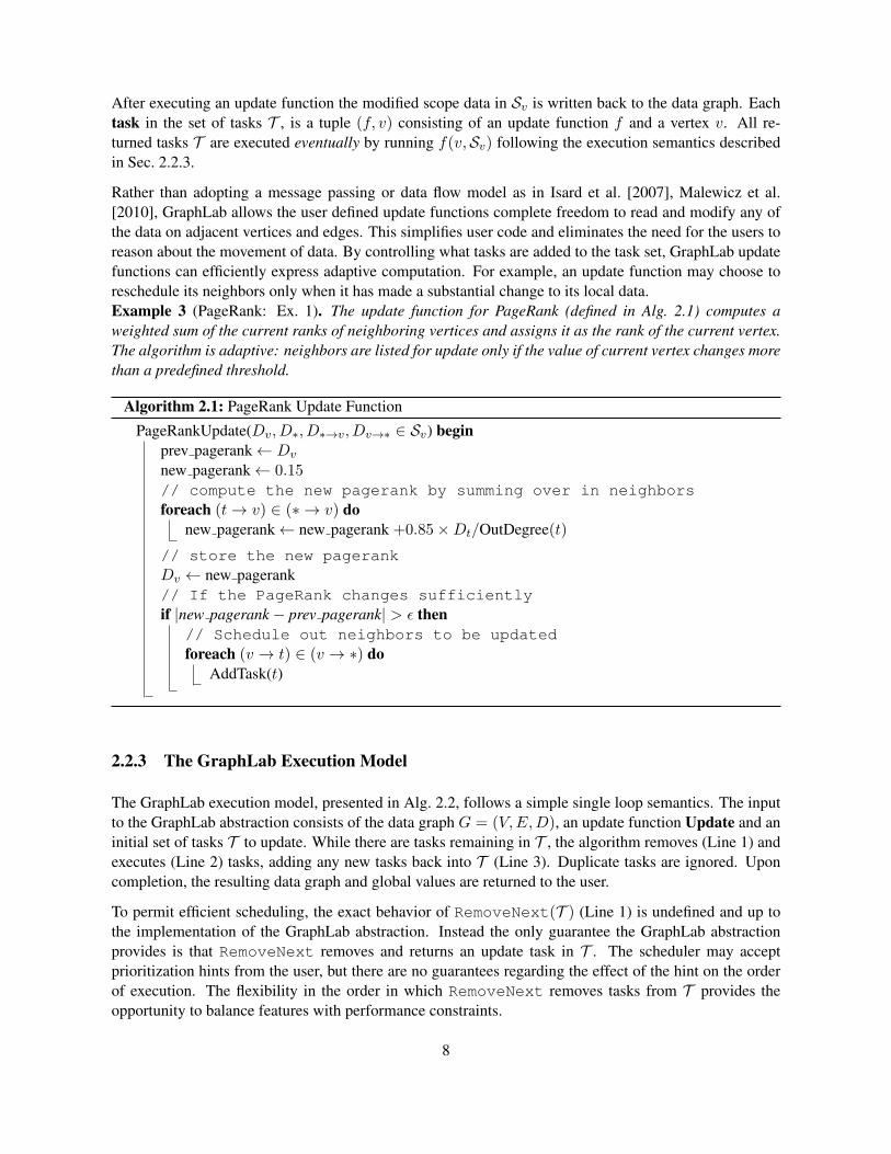
Algorithm 2.1: PageRank Update Function
PageRankUpdate(Dv, D∗, D∗→v, Dv→∗ ∈ Sv) beginprev pagerank← Dv
new pagerank← 0.15// compute the new pagerank by summing over in neighborsforeach (t→ v) ∈ (∗ → v) do
new pagerank← new pagerank +0.85×Dt/OutDegree(t)
// store the new pagerankDv ← new pagerank// If the PageRank changes sufficientlyif |new pagerank− prev pagerank| > ε then
// Schedule out neighbors to be updatedforeach (v → t) ∈ (v → ∗) do
AddTask(t)
2.2.3 The GraphLab Execution Model
The GraphLab execution model, presented in Alg. 2.2, follows a simple single loop semantics. The inputto the GraphLab abstraction consists of the data graph G = (V,E,D), an update function Update and aninitial set of tasks T to update. While there are tasks remaining in T , the algorithm removes (Line 1) andexecutes (Line 2) tasks, adding any new tasks back into T (Line 3). Duplicate tasks are ignored. Uponcompletion, the resulting data graph and global values are returned to the user.
To permit efficient scheduling, the exact behavior of RemoveNext(T ) (Line 1) is undefined and up tothe implementation of the GraphLab abstraction. Instead the only guarantee the GraphLab abstractionprovides is that RemoveNext removes and returns an update task in T . The scheduler may acceptprioritization hints from the user, but there are no guarantees regarding the effect of the hint on the orderof execution. The flexibility in the order in which RemoveNext removes tasks from T provides theopportunity to balance features with performance constraints.
8
Algorithm 2.2: GraphLab Execution ModelInput: Data Graph G = (V,E,D)Input: Initial task set T = {(f, v1), (g, v2), ...}while T is not Empty do
1 (f, v)← RemoveNext(T )2 (T ′,Sv)← f(v,Sv)3 T ← T ∪ T ′
Output: Modified Data Graph G = (V,E,D′)
2.2.4 Ensuring Serializability
An execution of the GraphLab abstraction must be able to enforce serializability. A serializable exe-cution of the GraphLab abstraction implies that there exists a corresponding serial schedule of updatefunctions that when executed by Alg. 2.2 produces the same data-graph. By ensuring serializable execu-tions, GraphLab simplifies reasoning about highly-asynchronous dynamic computation in the distributedsetting.
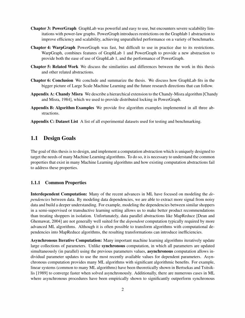
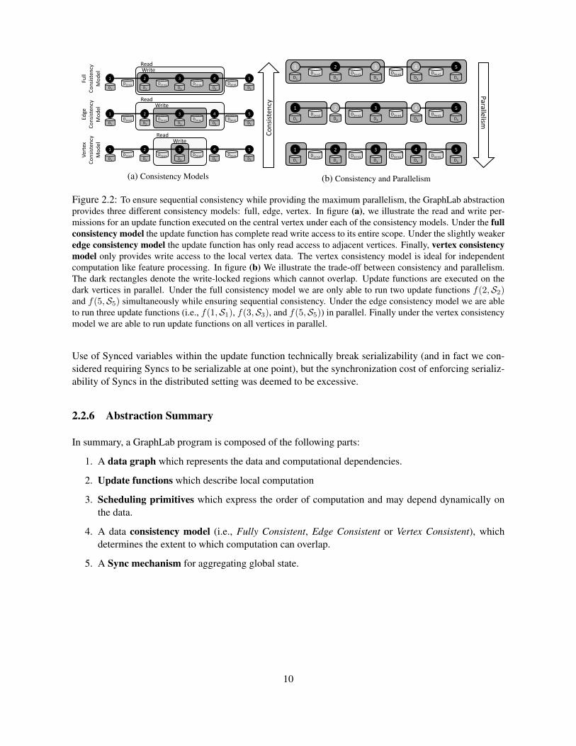
A simple method to achieve serializability is to ensure that the scopes of concurrently executing updatefunctions do not overlap. We call this the full consistency model (see Fig. 2.2a). However, full consistencylimits the potential parallelism since concurrently executing update functions must be at least two verticesapart (see Fig. 2.2b). However, for many machine learning algorithms, the update functions do not needfull read/write access to all of the data within the scope. For instance, the PageRank update in Eq. (2.1.1)only requires read access to edges and neighboring vertices. To provide greater parallelism while retainingserializability, GraphLab defines the edge consistency model. If the edge consistency model is used (seeFig. 2.2a), then each update function has exclusive read-write access to its vertex and adjacent edgesbut read only access to adjacent vertices. This increases parallelism by allowing update functions withslightly overlapping scopes to safely run in parallel (see Fig. 2.2b). Finally, the vertex consistency modelallows all update functions to be run in parallel, providing only consistent access to the scope’s centralvertex.
2.2.5 Sync Operation and Global Values
Finally, in many ML algorithms it is necessary to maintain global statistics describing data stored inthe data graph. For example, many statistical inference algorithms require tracking global convergenceestimators. To address this need, the GraphLab abstraction defines global values which may be read byupdate functions but are written using the sync operation. The sync operation, much like the aggregatesin Pregel, is an associative commutative operation:
Z = Finalize
(⊕v∈V
Map(Sv)
)(2.2.1)
defined over all the scopes in the graph. Note that the aggregate procedure includes a Finalize(·) operation,which is useful for performing final normalization (a common step in ML algorithms). The sync operationin GraphLab runs continuously in the background to maintain updated estimates of the global value.
9
Ver
tex
Co
nsi
sten
cy
Mo
del
Edge
Co
nsi
sten
cy
Mo
del
Full
Co
nsi
sten
cy
Mo
del
D1 D2 D3 D4 D5
D1↔2 D2↔3 D3↔4 D4↔5
1 2 3 4 5
WriteRead
D1 D2 D3 D4 D5
D1↔2 D2↔3 D3↔4 D4↔5
1 2 3 4 5
WriteRead
D1 D2 D3 D4 D5
D1↔2 D2↔3 D3↔4 D4↔5
1 2 3 4 5
WriteRead
(a) Consistency Models
D1 D2 D3 D4 D5
D1↔2 D2↔3 D3↔4 D4↔5
1 2 3 4 5
D1 D2 D3 D4 D5
D1↔2 D2↔3 D3↔4 D4↔5
1 2 3 4 5
D1 D2 D3 D4 D5
D1↔2 D2↔3 D3↔4 D4↔5
1 2 3 4 5
Co
nsi
sten
cy
Parallelism
(b) Consistency and Parallelism
Figure 2.2: To ensure sequential consistency while providing the maximum parallelism, the GraphLab abstractionprovides three different consistency models: full, edge, vertex. In figure (a), we illustrate the read and write per-missions for an update function executed on the central vertex under each of the consistency models. Under the fullconsistency model the update function has complete read write access to its entire scope. Under the slightly weakeredge consistency model the update function has only read access to adjacent vertices. Finally, vertex consistencymodel only provides write access to the local vertex data. The vertex consistency model is ideal for independentcomputation like feature processing. In figure (b) We illustrate the trade-off between consistency and parallelism.The dark rectangles denote the write-locked regions which cannot overlap. Update functions are executed on thedark vertices in parallel. Under the full consistency model we are only able to run two update functions f(2,S2)and f(5,S5) simultaneously while ensuring sequential consistency. Under the edge consistency model we are ableto run three update functions (i.e., f(1,S1), f(3,S3), and f(5,S5)) in parallel. Finally under the vertex consistencymodel we are able to run update functions on all vertices in parallel.
Use of Synced variables within the update function technically break serializability (and in fact we con-sidered requiring Syncs to be serializable at one point), but the synchronization cost of enforcing serializ-ability of Syncs in the distributed setting was deemed to be excessive.
2.2.6 Abstraction Summary
In summary, a GraphLab program is composed of the following parts:
1. A data graph which represents the data and computational dependencies.
2. Update functions which describe local computation
3. Scheduling primitives which express the order of computation and may depend dynamically onthe data.
4. A data consistency model (i.e., Fully Consistent, Edge Consistent or Vertex Consistent), whichdetermines the extent to which computation can overlap.
5. A Sync mechanism for aggregating global state.
10
2.3 Shared Memory Implementation
In Low et al. [2010], we implemented GraphLab for the shared memory setting. To summarize the results,we evaluated on five different problems: MRF Parameter Learning, Gibbs Sampling, CoEM, Lasso andCompressed sensing, and we demonstrated that the Shared Memory GraphLab implementation generallyachieves good performance, obtaining excellent strong scaling. The ability to choose between differentscheduler implementations (see Sec. 2.3.2), as well as the ability to pick between different consistencyguarantees permit a degree of adaptivity: allowing the user to pick the optimal scheduler, and the optimalconsistency level for his/her application.
To provide a basis for comparison of runtimes, we benchmarked our CoEM implementation to be 15xfaster than an equivalent Hadoop implementation while using only only 16 CPUs on a shared memorysystem, as compared to 95 CPUs on Hadoop.
Finally, the parallel Gibbs Sampler developed here was further extended in Gonzalez et al. [2011] toperform adaptive-block-Gibbs Sampling; once again showing excellent performance and scaling.
2.3.1 Engine
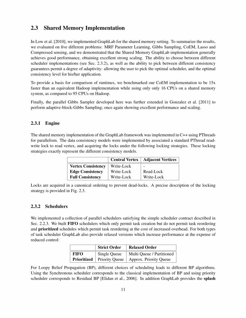
The shared memory implementation of the GraphLab framework was implemented in C++ using PThreadsfor parallelism. The data consistency models were implemented by associated a standard PThread read-write lock to read vertex, and acquiring the locks under the following locking strategies. These lockingstrategies exactly represent the different consistency models.
Central Vertex Adjacent VerticesVertex Consistency Write-Lock -Edge Consistency Write-Lock Read-LockFull Consistency Write-Lock Write-Lock
Locks are acquired in a canonical ordering to prevent dead-locks. A precise description of the lockingstrategy is provided in Fig. 2.3.
2.3.2 Schedulers
We implemented a collection of parallel schedulers satisfying the simple scheduler contract described inSec. 2.2.3. We built FIFO schedulers which only permit task creation but do not permit task reorderingand prioritized schedules which permit task reordering at the cost of increased overhead. For both typesof task scheduler GraphLab also provide relaxed versions which increase performance at the expense ofreduced control:
Strict Order Relaxed OrderFIFO Single Queue Multi Queue / PartitionedPrioritized Priority Queue Approx. Priority Queue
For Loopy Belief Propagation (BP), different choices of scheduling leads to different BP algorithms.Using the Synchronous scheduler corresponds to the classical implementation of BP and using priorityscheduler corresponds to Residual BP [Elidan et al., 2006]. In addition GraphLab provides the splash
11
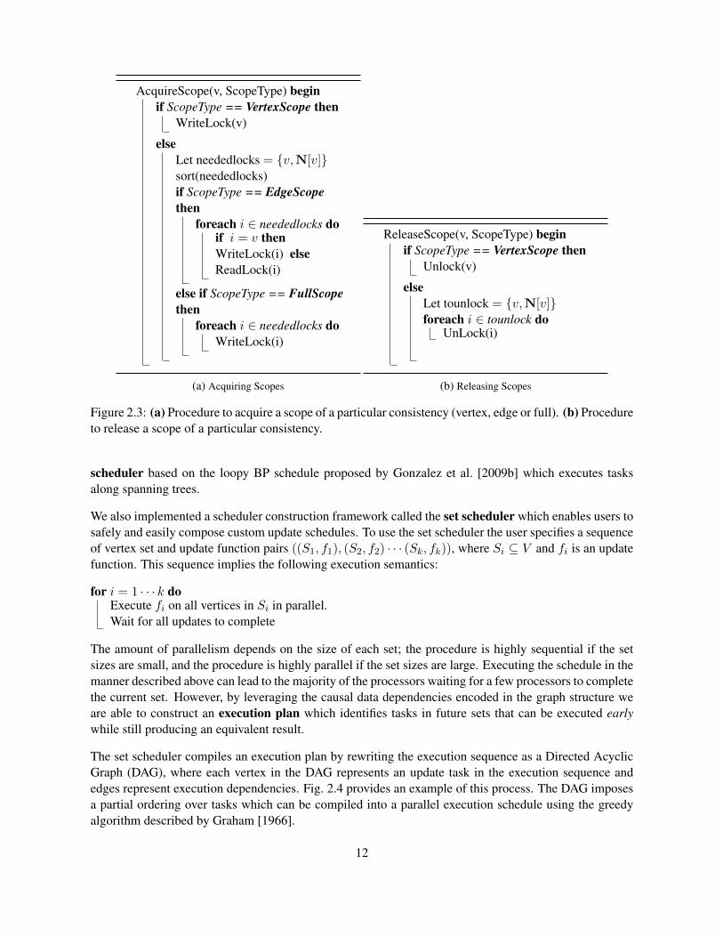
AcquireScope(v, ScopeType) beginif ScopeType == VertexScope then
WriteLock(v)
elseLet neededlocks = {v,N[v]}sort(neededlocks)if ScopeType == EdgeScopethen
foreach i ∈ neededlocks doif i = v thenWriteLock(i) elseReadLock(i)
else if ScopeType == FullScopethen
foreach i ∈ neededlocks doWriteLock(i)
(a) Acquiring Scopes
ReleaseScope(v, ScopeType) beginif ScopeType == VertexScope then
Unlock(v)
elseLet tounlock = {v,N[v]}foreach i ∈ tounlock do
UnLock(i)
(b) Releasing Scopes
Figure 2.3: (a) Procedure to acquire a scope of a particular consistency (vertex, edge or full). (b) Procedureto release a scope of a particular consistency.
scheduler based on the loopy BP schedule proposed by Gonzalez et al. [2009b] which executes tasksalong spanning trees.
We also implemented a scheduler construction framework called the set scheduler which enables users tosafely and easily compose custom update schedules. To use the set scheduler the user specifies a sequenceof vertex set and update function pairs ((S1, f1), (S2, f2) · · · (Sk, fk)), where Si ⊆ V and fi is an updatefunction. This sequence implies the following execution semantics:
for i = 1 · · · k doExecute fi on all vertices in Si in parallel.Wait for all updates to complete
The amount of parallelism depends on the size of each set; the procedure is highly sequential if the setsizes are small, and the procedure is highly parallel if the set sizes are large. Executing the schedule in themanner described above can lead to the majority of the processors waiting for a few processors to completethe current set. However, by leveraging the causal data dependencies encoded in the graph structure weare able to construct an execution plan which identifies tasks in future sets that can be executed earlywhile still producing an equivalent result.
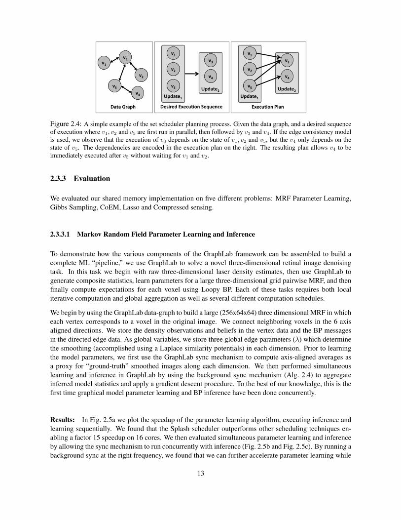
The set scheduler compiles an execution plan by rewriting the execution sequence as a Directed AcyclicGraph (DAG), where each vertex in the DAG represents an update task in the execution sequence andedges represent execution dependencies. Fig. 2.4 provides an example of this process. The DAG imposesa partial ordering over tasks which can be compiled into a parallel execution schedule using the greedyalgorithm described by Graham [1966].
12
vv1
Update1
vv2
vv5
vv3
Update2
vv4
Desired Execution Sequence
vv1
Update1
vv2
vv5
vv3
Update2
vv4
Execution Plan
vv1
vv3
vv5
vv4
vv2
Data Graph
Figure 2.4: A simple example of the set scheduler planning process. Given the data graph, and a desired sequenceof execution where v1, v2 and v5 are first run in parallel, then followed by v3 and v4. If the edge consistency modelis used, we observe that the execution of v3 depends on the state of v1, v2 and v5, but the v4 only depends on thestate of v5. The dependencies are encoded in the execution plan on the right. The resulting plan allows v4 to beimmediately executed after v5 without waiting for v1 and v2.
2.3.3 Evaluation
We evaluated our shared memory implementation on five different problems: MRF Parameter Learning,Gibbs Sampling, CoEM, Lasso and Compressed sensing.
2.3.3.1 Markov Random Field Parameter Learning and Inference
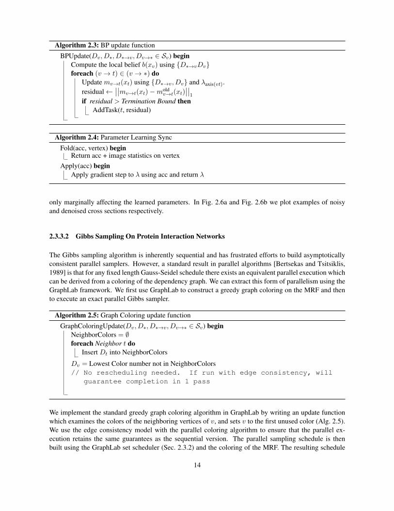
To demonstrate how the various components of the GraphLab framework can be assembled to build acomplete ML “pipeline,” we use GraphLab to solve a novel three-dimensional retinal image denoisingtask. In this task we begin with raw three-dimensional laser density estimates, then use GraphLab togenerate composite statistics, learn parameters for a large three-dimensional grid pairwise MRF, and thenfinally compute expectations for each voxel using Loopy BP. Each of these tasks requires both localiterative computation and global aggregation as well as several different computation schedules.
We begin by using the GraphLab data-graph to build a large (256x64x64) three dimensional MRF in whicheach vertex corresponds to a voxel in the original image. We connect neighboring voxels in the 6 axisaligned directions. We store the density observations and beliefs in the vertex data and the BP messagesin the directed edge data. As global variables, we store three global edge parameters (λ) which determinethe smoothing (accomplished using a Laplace similarity potentials) in each dimension. Prior to learningthe model parameters, we first use the GraphLab sync mechanism to compute axis-aligned averages asa proxy for “ground-truth” smoothed images along each dimension. We then performed simultaneouslearning and inference in GraphLab by using the background sync mechanism (Alg. 2.4) to aggregateinferred model statistics and apply a gradient descent procedure. To the best of our knowledge, this is thefirst time graphical model parameter learning and BP inference have been done concurrently.
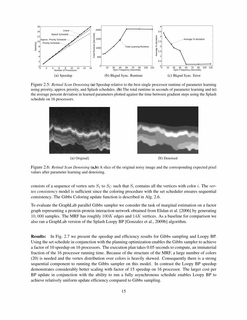
Results: In Fig. 2.5a we plot the speedup of the parameter learning algorithm, executing inference andlearning sequentially. We found that the Splash scheduler outperforms other scheduling techniques en-abling a factor 15 speedup on 16 cores. We then evaluated simultaneous parameter learning and inferenceby allowing the sync mechanism to run concurrently with inference (Fig. 2.5b and Fig. 2.5c). By running abackground sync at the right frequency, we found that we can further accelerate parameter learning while
13
Algorithm 2.3: BP update function
BPUpdate(Dv, D∗, D∗→v, Dv→∗ ∈ Sv) beginCompute the local belief b(xv) using {D∗→vDv}foreach (v → t) ∈ (v → ∗) do
Update mv→t(xt) using {D∗→v, Dv} and λaxis(vt).residual←
∣∣∣∣mv→t(xt)−moldv→t(xt)
∣∣∣∣1
if residual > Termination Bound thenAddTask(t, residual)
Algorithm 2.4: Parameter Learning Sync
Fold(acc, vertex) beginReturn acc + image statistics on vertex
Apply(acc) beginApply gradient step to λ using acc and return λ
only marginally affecting the learned parameters. In Fig. 2.6a and Fig. 2.6b we plot examples of noisyand denoised cross sections respectively.
2.3.3.2 Gibbs Sampling On Protein Interaction Networks
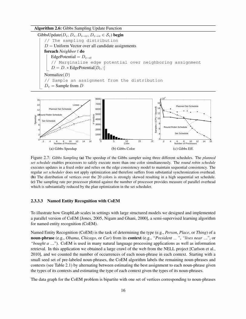
The Gibbs sampling algorithm is inherently sequential and has frustrated efforts to build asymptoticallyconsistent parallel samplers. However, a standard result in parallel algorithms [Bertsekas and Tsitsiklis,1989] is that for any fixed length Gauss-Seidel schedule there exists an equivalent parallel execution whichcan be derived from a coloring of the dependency graph. We can extract this form of parallelism using theGraphLab framework. We first use GraphLab to construct a greedy graph coloring on the MRF and thento execute an exact parallel Gibbs sampler.
Algorithm 2.5: Graph Coloring update function
GraphColoringUpdate(Dv, D∗, D∗→v, Dv→∗ ∈ Sv) beginNeighborColors = ∅foreach Neighbor t do
Insert Dt into NeighborColors
Dv = Lowest Color number not in NeighborColors// No rescheduling needed. If run with edge consistency, will
guarantee completion in 1 pass
We implement the standard greedy graph coloring algorithm in GraphLab by writing an update functionwhich examines the colors of the neighboring vertices of v, and sets v to the first unused color (Alg. 2.5).We use the edge consistency model with the parallel coloring algorithm to ensure that the parallel ex-ecution retains the same guarantees as the sequential version. The parallel sampling schedule is thenbuilt using the GraphLab set scheduler (Sec. 2.3.2) and the coloring of the MRF. The resulting schedule
14
0 2 4 6 8 10 12 14 160
2
4
6
8
10
12
14
16
Number of Processors
Spe
edup Priority Schedule
Approx. Priority Schedule
Linear
Splash Schedule
(a) Speedup
15 30 45 60 75 90 105 1200
500
1000
1500
2000
Sync Frequency (Seconds)
Tot
al R
untim
e (S
econ
ds)
Total Learning Runtime
(b) Bkgnd Sync. Runtime
0 15 30 45 60 75 90 105 1200
0.5
1
1.5
2
2.5
3
3.5
4
Sync Frequency (Seconds)
Ave
rage
% d
evia
tion
Average % deviation
(c) Bkgnd Sync. Error
Figure 2.5: Retinal Scan Denoising (a) Speedup relative to the best single processor runtime of parameter learningusing priority, approx priority, and Splash schedules. (b) The total runtime in seconds of parameter learning and (c)the average percent deviation in learned parameters plotted against the time between gradient steps using the Splashschedule on 16 processors.
(a) Original] (b) Denoised
Figure 2.6: Retinal Scan Denoising (a,b) A slice of the original noisy image and the corresponding expected pixelvalues after parameter learning and denoising.
consists of a sequence of vertex sets S1 to SC such that Si contains all the vertices with color i. The ver-tex consistency model is sufficient since the coloring procedure with the set scheduler ensures sequentialconsistency. The Gibbs Coloring update function is described in Alg. 2.6.
To evaluate the GraphLab parallel Gibbs sampler we consider the task of marginal estimation on a factorgraph representing a protein-protein interaction network obtained from Elidan et al. [2006] by generating10, 000 samples. The MRF has roughly 100K edges and 14K vertices. As a baseline for comparison wealso ran a GraphLab version of the Splash Loopy BP [Gonzalez et al., 2009b] algorithm.
Results: In Fig. 2.7 we present the speedup and efficiency results for Gibbs sampling and Loopy BP.Using the set schedule in conjunction with the planning optimization enables the Gibbs sampler to achievea factor of 10 speedup on 16 processors. The execution plan takes 0.05 seconds to compute, an immaterialfraction of the 16 processor running time. Because of the structure of the MRF, a large number of colors(20) is needed and the vertex distribution over colors is heavily skewed. Consequently there is a strongsequential component to running the Gibbs sampler on this model. In contrast the Loopy BP speedupdemonstrates considerably better scaling with factor of 15 speedup on 16 processor. The larger cost perBP update in conjunction with the ability to run a fully asynchronous schedule enables Loopy BP toachieve relatively uniform update efficiency compared to Gibbs sampling.
15
Algorithm 2.6: Gibbs Sampling Update Function
GibbsUpdate(Dv, D∗, D∗→v, Dv→∗ ∈ Sv) begin// The sampling distributionD = Uniform Vector over all candidate assignmentsforeach Neighbor t do
EdgePotential = Dv→t// Marginalize edge potential over neighboring assignmentD = D. ∗ EdgePotential[Dt, :]
Normalize(D)// Sample an assignment from the distributionDv = Sample from D
2 4 6 8 10 12 14 160
2
4
6
8
10
12
14
16
Number of Processors
Spe
edup
Linear
Planned Set Schedule
Round Robin Schedule
Set Schedule
(a) Gibbs Speedup
0 5 10 15 200
1000
2000
3000
4000
5000
6000
7000
8000
Color
# V
ertic
es
(b) Gibbs Color
2 4 6 8 10 12 14 162
4
6
8
10
12
14
16
x 104
Number of Processors
Sam
ples
/ (C
PU
* S
econ
d)
Planned Set Schedule
Round Robin Schedule
Set Schedule
(c) Gibbs Eff.
Figure 2.7: Gibbs Sampling (a) The speedup of the Gibbs sampler using three different schedules. The plannedset schedule enables processors to safely execute more than one color simultaneously. The round robin scheduleexecutes updates in a fixed order and relies on the edge consistency model to maintain sequential consistency. Theregular set scheduler does not apply optimization and therefore suffers from substantial synchronization overhead.(b) The distribution of vertices over the 20 colors is strongly skewed resulting in a high sequential set schedule.(c) The sampling rate per processor plotted against the number of processor provides measure of parallel overheadwhich is substantially reduced by the plan optimization in the set scheduler.
2.3.3.3 Named Entity Recognition with CoEM
To illustrate how GraphLab scales in settings with large structured models we designed and implementeda parallel version of CoEM [Jones, 2005, Nigam and Ghani, 2000], a semi-supervised learning algorithmfor named entity recognition (CoEM).
Named Entity Recognition (CoEM) is the task of determining the type (e.g., Person, Place, or Thing) of anoun-phrase (e.g., Obama, Chicago, or Car) from its context (e.g., “President ”, “lives near .”, or“bought a .”). CoEM is used in many natural language processing applications as well as informationretrieval. In this application we obtained a large crawl of the web from the NELL project [Carlson et al.,2010], and we counted the number of occurrences of each noun-phrase in each context. Starting with asmall seed set of pre-labeled noun-phrases, the CoEM algorithm labels the remaining noun-phrases andcontexts (see Table 2.1) by alternating between estimating the best assignment to each noun-phrase giventhe types of its contexts and estimating the type of each context given the types of its noun-phrases.
The data graph for the CoEM problem is bipartite with one set of vertices corresponding to noun-phrases
16
2 4 6 8 10 12 14 160
2
4
6
8
10
12
14
16
Number of Processors
Spe
edup
Linear
Splash Schedule
Residual Schedule
(a) BP Speedup
2 4 6 8 10 12 14 16
1.9
2
2.1
2.2
2.3
2.4
2.5
x 104
Number of Processors
Upd
ates
/ (C
PU
* S
econ
d)
Splash Schedule
Residual Schedule
(b) BP Eff.
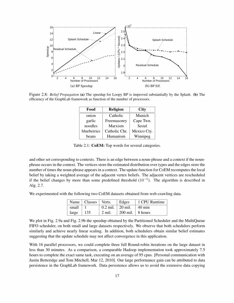
Figure 2.8: Belief Propagation (a) The speedup for Loopy BP is improved substantially by the Splash. (b) Theefficiency of the GraphLab framework as function of the number of processors.
Food Religion Cityonion Catholic Munichgarlic Freemasonry Cape Twn.
noodles Marxism Seoulblueberries Catholic Chr. Mexico Cty.
beans Humanism Winnipeg
Table 2.1: CoEM: Top words for several categories.
and other set corresponding to contexts. There is an edge between a noun-phrase and a context if the noun-phrase occurs in the context. The vertices store the estimated distribution over types and the edges store thenumber of times the noun-phrase appears in a context. The update function for CoEM recomputes the localbelief by taking a weighted average of the adjacent vertex beliefs. The adjacent vertices are rescheduledif the belief changes by more than some predefined threshold (10−5). The algorithm is described inAlg. 2.7.
We experimented with the following two CoEM datasets obtained from web-crawling data.
Name Classes Verts. Edges 1 CPU Runtimesmall 1 0.2 mil. 20 mil. 40 minlarge 135 2 mil. 200 mil. 8 hours
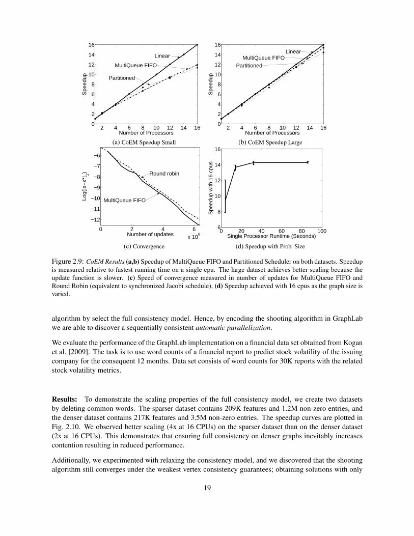
We plot in Fig. 2.9a and Fig. 2.9b the speedup obtained by the Partitioned Scheduler and the MultiQueueFIFO scheduler, on both small and large datasets respectively. We observe that both schedulers performsimilarly and achieve nearly linear scaling. In addition, both schedulers obtain similar belief estimatessuggesting that the update schedule may not affect convergence in this application.
With 16 parallel processors, we could complete three full Round-robin iterations on the large dataset inless than 30 minutes. As a comparison, a comparable Hadoop implementation took approximately 7.5hours to complete the exact same task, executing on an average of 95 cpus. [Personal communication withJustin Betteridge and Tom Mitchell, Mar 12, 2010]. Our large performance gain can be attributed to datapersistence in the GraphLab framework. Data persistence allows us to avoid the extensive data copying
17
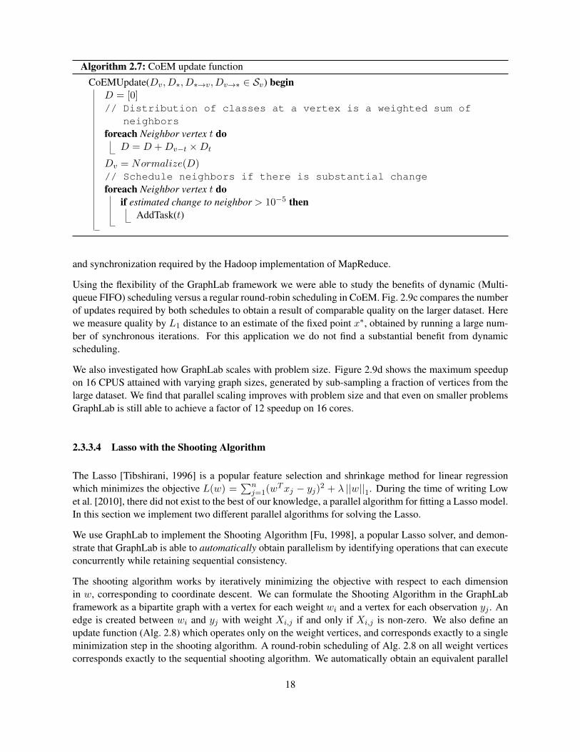
Algorithm 2.7: CoEM update function
CoEMUpdate(Dv, D∗, D∗→v, Dv→∗ ∈ Sv) beginD = [0]// Distribution of classes at a vertex is a weighted sum of
neighborsforeach Neighbor vertex t do
D = D +Dv−t ×Dt
Dv = Normalize(D)// Schedule neighbors if there is substantial changeforeach Neighbor vertex t do
if estimated change to neighbor > 10−5 thenAddTask(t)
and synchronization required by the Hadoop implementation of MapReduce.
Using the flexibility of the GraphLab framework we were able to study the benefits of dynamic (Multi-queue FIFO) scheduling versus a regular round-robin scheduling in CoEM. Fig. 2.9c compares the numberof updates required by both schedules to obtain a result of comparable quality on the larger dataset. Herewe measure quality by L1 distance to an estimate of the fixed point x∗, obtained by running a large num-ber of synchronous iterations. For this application we do not find a substantial benefit from dynamicscheduling.
We also investigated how GraphLab scales with problem size. Figure 2.9d shows the maximum speedupon 16 CPUS attained with varying graph sizes, generated by sub-sampling a fraction of vertices from thelarge dataset. We find that parallel scaling improves with problem size and that even on smaller problemsGraphLab is still able to achieve a factor of 12 speedup on 16 cores.
2.3.3.4 Lasso with the Shooting Algorithm
The Lasso [Tibshirani, 1996] is a popular feature selection and shrinkage method for linear regressionwhich minimizes the objective L(w) =
∑nj=1(w
Txj − yj)2 + λ ||w||1. During the time of writing Lowet al. [2010], there did not exist to the best of our knowledge, a parallel algorithm for fitting a Lasso model.In this section we implement two different parallel algorithms for solving the Lasso.
We use GraphLab to implement the Shooting Algorithm [Fu, 1998], a popular Lasso solver, and demon-strate that GraphLab is able to automatically obtain parallelism by identifying operations that can executeconcurrently while retaining sequential consistency.
The shooting algorithm works by iteratively minimizing the objective with respect to each dimensionin w, corresponding to coordinate descent. We can formulate the Shooting Algorithm in the GraphLabframework as a bipartite graph with a vertex for each weight wi and a vertex for each observation yj . Anedge is created between wi and yj with weight Xi,j if and only if Xi,j is non-zero. We also define anupdate function (Alg. 2.8) which operates only on the weight vertices, and corresponds exactly to a singleminimization step in the shooting algorithm. A round-robin scheduling of Alg. 2.8 on all weight verticescorresponds exactly to the sequential shooting algorithm. We automatically obtain an equivalent parallel
18
2 4 6 8 10 12 14 160
2
4
6
8
10
12
14
16
Number of Processors
Spe
edup
Linear
MultiQueue FIFO
Partitioned
(a) CoEM Speedup Small
2 4 6 8 10 12 14 160
2
4
6
8
10
12
14
16
Number of Processors
Spe
edup
LinearMultiQueue FIFO
Partitioned
(b) CoEM Speedup Large
0 2 4 6x 10
6
−12
−11
−10
−9
−8
−7
−6
Number of updates
Log(
|x−
x*| 1) Round robin
MultiQueue FIFO
(c) Convergence
0 20 40 60 80 1006
8
10
12
14
16
Single Processor Runtime (Seconds)
Spe
edup
with
16
cpus
(d) Speedup with Prob. Size
Figure 2.9: CoEM Results (a,b) Speedup of MultiQueue FIFO and Partitioned Scheduler on both datasets. Speedupis measured relative to fastest running time on a single cpu. The large dataset achieves better scaling because theupdate function is slower. (c) Speed of convergence measured in number of updates for MultiQueue FIFO andRound Robin (equivalent to synchronized Jacobi schedule), (d) Speedup achieved with 16 cpus as the graph size isvaried.
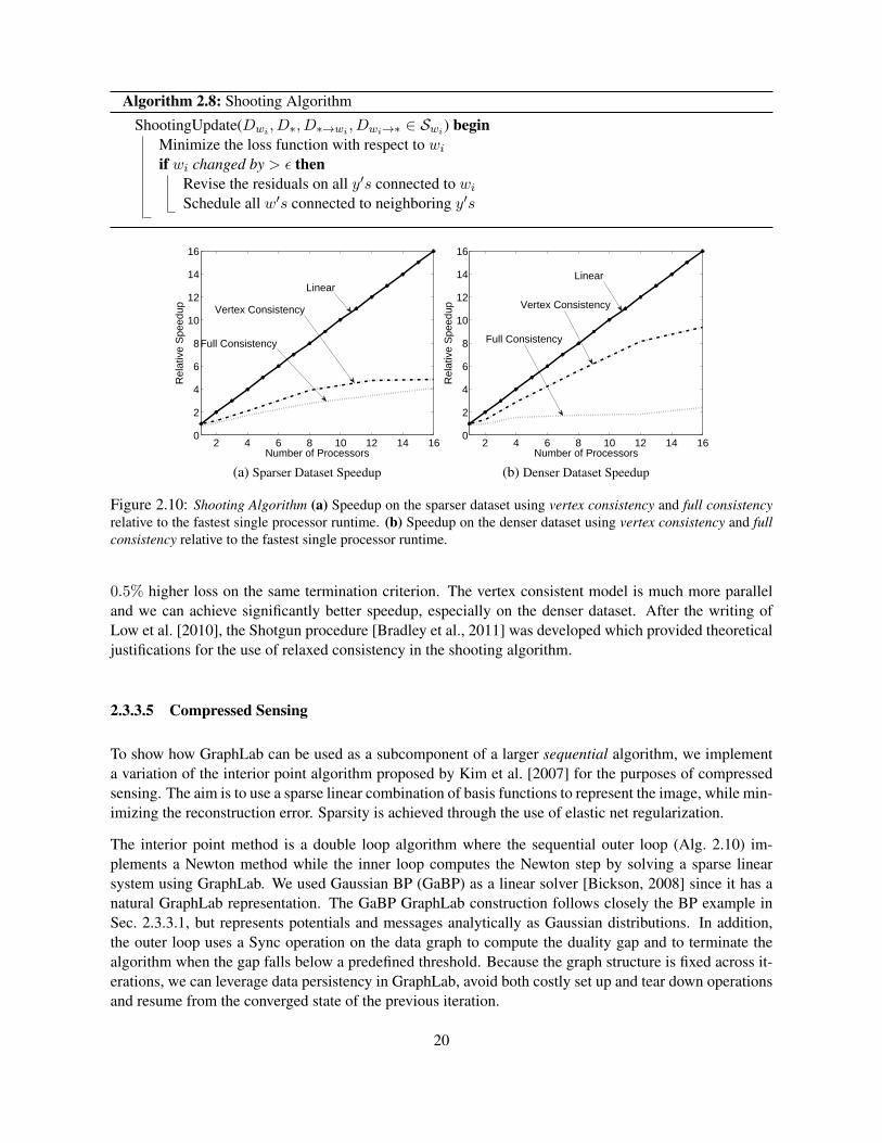
algorithm by select the full consistency model. Hence, by encoding the shooting algorithm in GraphLabwe are able to discover a sequentially consistent automatic parallelization.
We evaluate the performance of the GraphLab implementation on a financial data set obtained from Koganet al. [2009]. The task is to use word counts of a financial report to predict stock volatility of the issuingcompany for the consequent 12 months. Data set consists of word counts for 30K reports with the relatedstock volatility metrics.
Results: To demonstrate the scaling properties of the full consistency model, we create two datasetsby deleting common words. The sparser dataset contains 209K features and 1.2M non-zero entries, andthe denser dataset contains 217K features and 3.5M non-zero entries. The speedup curves are plotted inFig. 2.10. We observed better scaling (4x at 16 CPUs) on the sparser dataset than on the denser dataset(2x at 16 CPUs). This demonstrates that ensuring full consistency on denser graphs inevitably increasescontention resulting in reduced performance.
Additionally, we experimented with relaxing the consistency model, and we discovered that the shootingalgorithm still converges under the weakest vertex consistency guarantees; obtaining solutions with only
19
Algorithm 2.8: Shooting Algorithm
ShootingUpdate(Dwi , D∗, D∗→wi , Dwi→∗ ∈ Swi) beginMinimize the loss function with respect to wiif wi changed by > ε then
Revise the residuals on all y′s connected to wiSchedule all w′s connected to neighboring y′s
2 4 6 8 10 12 14 160
2
4
6
8
10
12
14
16
Number of Processors
Rel
ativ
e S
peed
up
Linear
Full Consistency
Vertex Consistency
(a) Sparser Dataset Speedup
2 4 6 8 10 12 14 160
2
4
6
8
10
12
14
16
Number of ProcessorsR
elat
ive
Spe
edup
Full Consistency
Vertex Consistency
Linear
(b) Denser Dataset Speedup
Figure 2.10: Shooting Algorithm (a) Speedup on the sparser dataset using vertex consistency and full consistencyrelative to the fastest single processor runtime. (b) Speedup on the denser dataset using vertex consistency and fullconsistency relative to the fastest single processor runtime.
0.5% higher loss on the same termination criterion. The vertex consistent model is much more paralleland we can achieve significantly better speedup, especially on the denser dataset. After the writing ofLow et al. [2010], the Shotgun procedure [Bradley et al., 2011] was developed which provided theoreticaljustifications for the use of relaxed consistency in the shooting algorithm.
2.3.3.5 Compressed Sensing
To show how GraphLab can be used as a subcomponent of a larger sequential algorithm, we implementa variation of the interior point algorithm proposed by Kim et al. [2007] for the purposes of compressedsensing. The aim is to use a sparse linear combination of basis functions to represent the image, while min-imizing the reconstruction error. Sparsity is achieved through the use of elastic net regularization.
The interior point method is a double loop algorithm where the sequential outer loop (Alg. 2.10) im-plements a Newton method while the inner loop computes the Newton step by solving a sparse linearsystem using GraphLab. We used Gaussian BP (GaBP) as a linear solver [Bickson, 2008] since it has anatural GraphLab representation. The GaBP GraphLab construction follows closely the BP example inSec. 2.3.3.1, but represents potentials and messages analytically as Gaussian distributions. In addition,the outer loop uses a Sync operation on the data graph to compute the duality gap and to terminate thealgorithm when the gap falls below a predefined threshold. Because the graph structure is fixed across it-erations, we can leverage data persistency in GraphLab, avoid both costly set up and tear down operationsand resume from the converged state of the previous iteration.
20
2 4 6 8 10 12 14 160
2
4
6
8
10
12
14
16
Number of Processors
Spe
edup
Linear
L1 Interior Point
(a) Speedup (b) Lenna (c) Lenna 50%
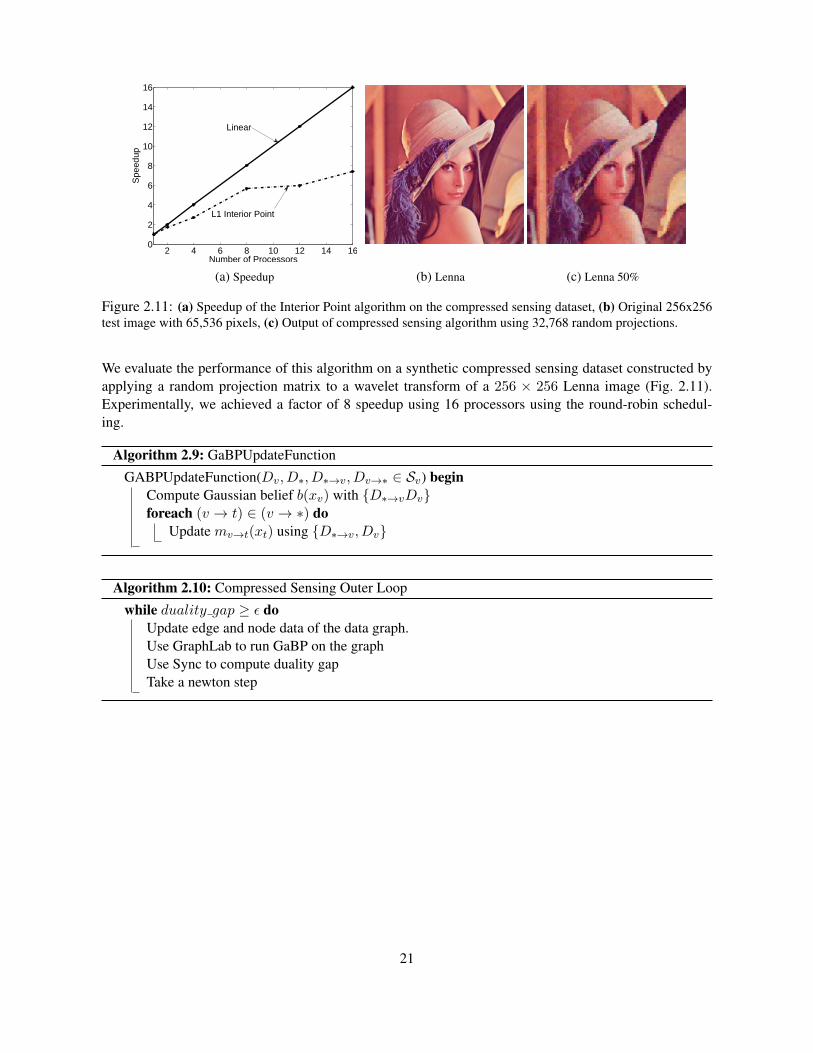
Figure 2.11: (a) Speedup of the Interior Point algorithm on the compressed sensing dataset, (b) Original 256x256test image with 65,536 pixels, (c) Output of compressed sensing algorithm using 32,768 random projections.
We evaluate the performance of this algorithm on a synthetic compressed sensing dataset constructed byapplying a random projection matrix to a wavelet transform of a 256 × 256 Lenna image (Fig. 2.11).Experimentally, we achieved a factor of 8 speedup using 16 processors using the round-robin schedul-ing.
Algorithm 2.9: GaBPUpdateFunction
GABPUpdateFunction(Dv, D∗, D∗→v, Dv→∗ ∈ Sv) beginCompute Gaussian belief b(xv) with {D∗→vDv}foreach (v → t) ∈ (v → ∗) do
Update mv→t(xt) using {D∗→v, Dv}
Algorithm 2.10: Compressed Sensing Outer Loop
while duality gap ≥ ε doUpdate edge and node data of the data graph.Use GraphLab to run GaBP on the graphUse Sync to compute duality gapTake a newton step
21
2.4 Distributed Implementation
The usefulness of the shared memory GraphLab system, encouraged us to provide greater scalability andperformance by extending to the distributed setting [Low et al., 2012]. In this section, we discuss thetechniques required to achieve this goal. We focus on in distributed in-memory setting, requiring theentire graph and all program state to reside in distributed RAM. Our distributed implementation is writtenin C++ and extends the previous shared memory GraphLab implementation.
The key challenges in extending the shared memory implementation to the distributed setting are:
State Partitioning How to efficiently load, partition and distribute the data graph across machines. Weaddress this using a two-phase partitioning procedure described in Sec. 2.4.1.
Consistency The GraphLab abstraction specifies three grades of computation consistency: i.e. vertex,edge, and full consistency (Sec. 2.2.4). While consistency is easy to implement in the shared mem-ory setting, achieving consistency in the distributed setting is substantially more difficult. We dis-cuss two solutions in the Engines section Sec. 2.4.2.
Fault Tolerance Snapshotting is a common scheme for achieving fault tolerance in the distributed setting.While “stop the world” snapshots are always feasible, the sparse computation structure of GraphLabpermits the use of an asynchronous snapshot procedure which we describe in Sec. 2.4.3.
2.4.1 The Data Graph
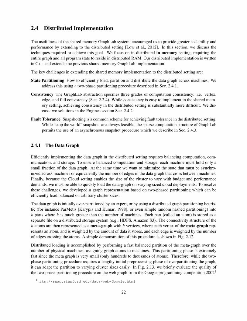
Efficiently implementing the data graph in the distributed setting requires balancing computation, com-munication, and storage. To ensure balanced computation and storage, each machine must hold only asmall fraction of the data graph. At the same time we want to minimize the state that must be synchro-nized across machines or equivalently the number of edges in the data graph that cross between machines.Finally, because the Cloud setting enables the size of the cluster to vary with budget and performancedemands, we must be able to quickly load the data-graph on varying sized cloud deployments. To resolvethese challenges, we developed a graph representation based on two-phased partitioning which can beefficiently load balanced on arbitrary cluster sizes.
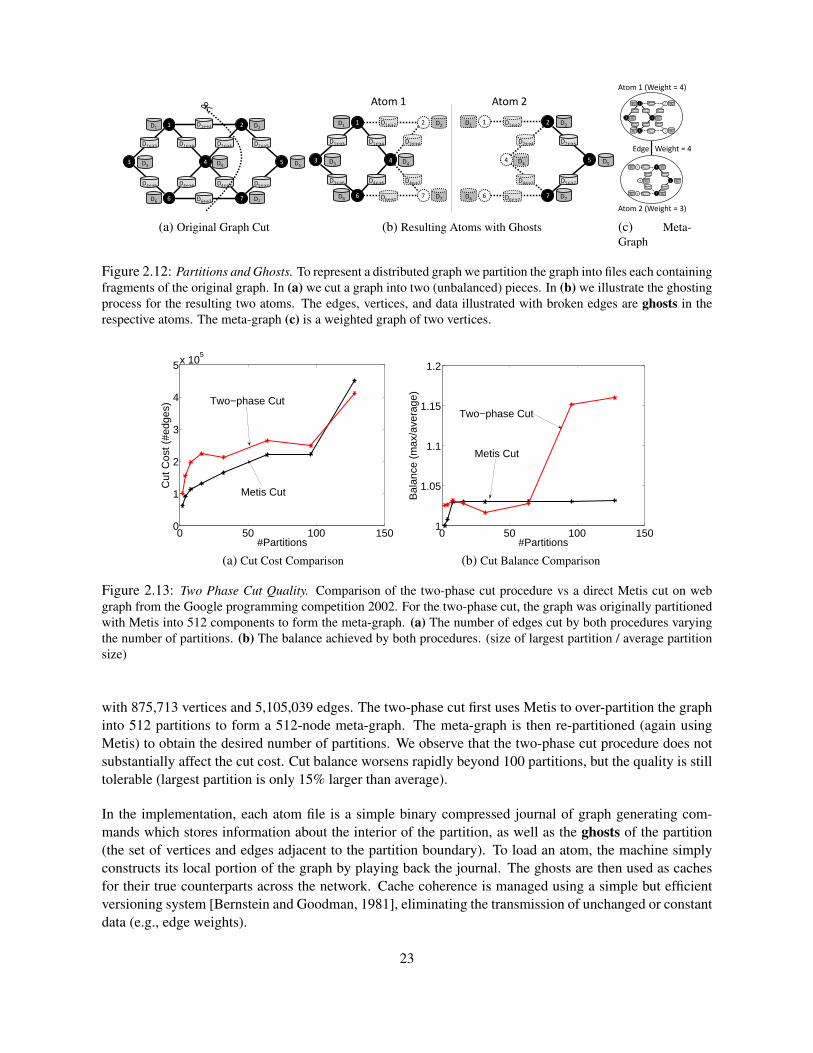
The data graph is initially over-partitioned by an expert, or by using a distributed graph partitioning heuris-tic (for instance ParMetis [Karypis and Kumar, 1998], or even simple random hashed partitioning) intok parts where k is much greater than the number of machines. Each part (called an atom) is stored as aseparate file on a distributed storage system (e.g., HDFS, Amazon S3). The connectivity structure of thek atoms are then represented as a meta-graph with k vertices, where each vertex of the meta-graph rep-resents an atom, and is weighted by the amount of data it stores, and each edge is weighted by the numberof edges crossing the atoms. A simple demonstration of this procedure is shown in Fig. 2.12.
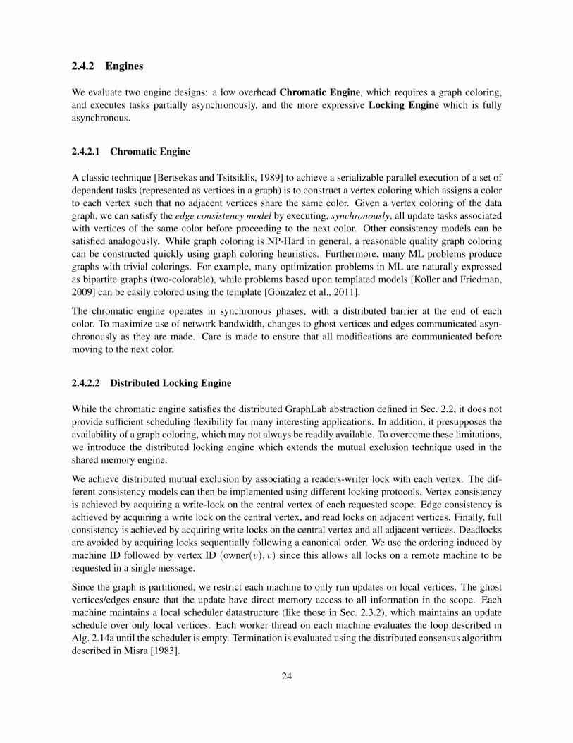
Distributed loading is accomplished by performing a fast balanced partition of the meta-graph over thenumber of physical machines, assigning graph atoms to machines. This partitioning phase is extremelyfast since the meta graph is very small (only hundreds to thousands of atoms). Therefore, while the two-phase partitioning procedure requires a lengthy initial preprocessing phase of overpartitioning the graph,it can adapt the partition to varying cluster sizes easily. In Fig. 2.13, we briefly evaluate the quality ofthe two-phase partitioning procedure on the web graph from the Google programming competition 20021
1http://snap.stanford.edu/data/web-Google.html
22
4
D1
6
1 2
7
D1↔2
D2↔4D1↔3
D6↔7
53
D2
D3 D4 D5
D6 D7
D1↔4 D2↔5
D4↔7D3↔6 D4↔6 D5↔7
(a) Original Graph Cut
4
D1
6
1 2
7
D1↔3
3
D2
D3 D4
D6 D7
D1↔4
D3↔6 D4↔6
4
D1
6
1 2
7
5
D2
D4 D5
D6 D7
D2↔5
D5↔7
Atom 1 Atom 2
D1↔2
D2↔4
D6↔7
D4↔7
D1↔2
D2↔4
D6↔7
D4↔7
(b) Resulting Atoms with Ghosts
Atom 1 (Weight = 4)
Atom 2 (Weight = 3)
4
D1
6
1 2
7
5
D2
D4 D5
D6 D7
D2↔5
D5↔7
D1↔2
D2↔4
D6↔7
D4↔7
4
D1
6
1 2
7
D1↔3
3
D2
D3 D4
D6 D7
D1↔4
D3↔6 D4↔6
D1↔2
D2↔4
D6↔7
D4↔7
Edge Weight = 4
(c) Meta-Graph
Figure 2.12: Partitions and Ghosts. To represent a distributed graph we partition the graph into files each containingfragments of the original graph. In (a) we cut a graph into two (unbalanced) pieces. In (b) we illustrate the ghostingprocess for the resulting two atoms. The edges, vertices, and data illustrated with broken edges are ghosts in therespective atoms. The meta-graph (c) is a weighted graph of two vertices.
0 50 100 1500
1
2
3
4
5x 10⁵
#Partitions
Cut
Cos
t (#e
dges
) Two−phase Cut
Metis Cut
(a) Cut Cost Comparison
0 50 100 1501
1.05
1.1
1.15
1.2
#Partitions
Bal
ance
(m
ax/a
vera
ge)
Two−phase Cut
Metis Cut
(b) Cut Balance Comparison
Figure 2.13: Two Phase Cut Quality. Comparison of the two-phase cut procedure vs a direct Metis cut on webgraph from the Google programming competition 2002. For the two-phase cut, the graph was originally partitionedwith Metis into 512 components to form the meta-graph. (a) The number of edges cut by both procedures varyingthe number of partitions. (b) The balance achieved by both procedures. (size of largest partition / average partitionsize)
with 875,713 vertices and 5,105,039 edges. The two-phase cut first uses Metis to over-partition the graphinto 512 partitions to form a 512-node meta-graph. The meta-graph is then re-partitioned (again usingMetis) to obtain the desired number of partitions. We observe that the two-phase cut procedure does notsubstantially affect the cut cost. Cut balance worsens rapidly beyond 100 partitions, but the quality is stilltolerable (largest partition is only 15% larger than average).
In the implementation, each atom file is a simple binary compressed journal of graph generating com-mands which stores information about the interior of the partition, as well as the ghosts of the partition(the set of vertices and edges adjacent to the partition boundary). To load an atom, the machine simplyconstructs its local portion of the graph by playing back the journal. The ghosts are then used as cachesfor their true counterparts across the network. Cache coherence is managed using a simple but efficientversioning system [Bernstein and Goodman, 1981], eliminating the transmission of unchanged or constantdata (e.g., edge weights).
23
2.4.2 Engines
We evaluate two engine designs: a low overhead Chromatic Engine, which requires a graph coloring,and executes tasks partially asynchronously, and the more expressive Locking Engine which is fullyasynchronous.
2.4.2.1 Chromatic Engine
A classic technique [Bertsekas and Tsitsiklis, 1989] to achieve a serializable parallel execution of a set ofdependent tasks (represented as vertices in a graph) is to construct a vertex coloring which assigns a colorto each vertex such that no adjacent vertices share the same color. Given a vertex coloring of the datagraph, we can satisfy the edge consistency model by executing, synchronously, all update tasks associatedwith vertices of the same color before proceeding to the next color. Other consistency models can besatisfied analogously. While graph coloring is NP-Hard in general, a reasonable quality graph coloringcan be constructed quickly using graph coloring heuristics. Furthermore, many ML problems producegraphs with trivial colorings. For example, many optimization problems in ML are naturally expressedas bipartite graphs (two-colorable), while problems based upon templated models [Koller and Friedman,2009] can be easily colored using the template [Gonzalez et al., 2011].
The chromatic engine operates in synchronous phases, with a distributed barrier at the end of eachcolor. To maximize use of network bandwidth, changes to ghost vertices and edges communicated asyn-chronously as they are made. Care is made to ensure that all modifications are communicated beforemoving to the next color.
2.4.2.2 Distributed Locking Engine
While the chromatic engine satisfies the distributed GraphLab abstraction defined in Sec. 2.2, it does notprovide sufficient scheduling flexibility for many interesting applications. In addition, it presupposes theavailability of a graph coloring, which may not always be readily available. To overcome these limitations,we introduce the distributed locking engine which extends the mutual exclusion technique used in theshared memory engine.
We achieve distributed mutual exclusion by associating a readers-writer lock with each vertex. The dif-ferent consistency models can then be implemented using different locking protocols. Vertex consistencyis achieved by acquiring a write-lock on the central vertex of each requested scope. Edge consistency isachieved by acquiring a write lock on the central vertex, and read locks on adjacent vertices. Finally, fullconsistency is achieved by acquiring write locks on the central vertex and all adjacent vertices. Deadlocksare avoided by acquiring locks sequentially following a canonical order. We use the ordering induced bymachine ID followed by vertex ID (owner(v), v) since this allows all locks on a remote machine to berequested in a single message.
Since the graph is partitioned, we restrict each machine to only run updates on local vertices. The ghostvertices/edges ensure that the update have direct memory access to all information in the scope. Eachmachine maintains a local scheduler datastructure (like those in Sec. 2.3.2), which maintains an updateschedule over only local vertices. Each worker thread on each machine evaluates the loop described inAlg. 2.14a until the scheduler is empty. Termination is evaluated using the distributed consensus algorithmdescribed in Misra [1983].
24
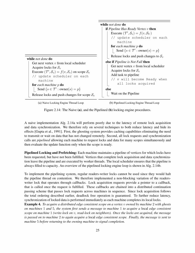
while not done doGet next vertex v from local schedulerAcquire locks for SvExecute (T ′,Sv) = f(v,Sv) on scope Sv// update scheduler on each
machinefor each machine p do
Send {s ∈ T ′ : owner(s) = p}Release locks and push changes for scope Sv
(a) Naive Locking Engine Thread Loop
while not done doif Pipeline Has Ready Vertex v then
Execute (T ′,Sv) = f(v,SV )// update scheduler on each
machinefor each machine p do
Send {s ∈ T ′ : owner(s) = p}Release locks and push changes to Sv
else if Pipeline is Not Full thenGet next vertex v from local schedulerAcquire locks for SvAdd task to pipeline// v will become Ready when
all locks acquired
elseWait on the Pipeline
(b) Pipelined Locking Engine Thread Loop
Figure 2.14: The Naive (a), and the Pipelined (b) locking engine procedures.
A naive implementation Alg. 2.14a will perform poorly due to the latency of remote lock acquisitionand data synchronization. We therefore rely on several techniques to both reduce latency and hide itseffects [Gupta et al., 1991]. First, the ghosting system provides caching capabilities eliminating the needto transmit or wait on data that has not changed remotely. Second, all lock requests and synchronizationcalls are pipelined allowing each machine to request locks and data for many scopes simultaneously andthen evaluate the update function only when the scope is ready.
Pipelined Locking and Prefetching: Each machine maintains a pipeline of vertices for which locks havebeen requested, but have not been fulfilled. Vertices that complete lock acquisition and data synchroniza-tion leave the pipeline and are executed by worker threads. The local scheduler ensures that the pipeline isalways filled to capacity. An overview of the pipelined locking engine loop is shown in Alg. 2.14b.
To implement the pipelining system, regular readers-writer locks cannot be used since they would haltthe pipeline thread on contention. We therefore implemented a non-blocking variation of the readers-writer lock that operates through callbacks. Lock acquisition requests provide a pointer to a callback,that is called once the request is fulfilled. These callbacks are chained into a distributed continuationpassing scheme that passes lock requests across machines in sequence. Since lock acquisition followsthe total ordering described earlier, deadlock free operation is guaranteed. To further reduce latency,synchronization of locked data is performed immediately as each machine completes its local locks.Example 4. To acquire a distributed edge consistent scope on a vertex v owned by machine 2 with ghostson machines 1 and 5, the system first sends a message to machine 1 to acquire a local edge consistentscope on machine 1 (write-lock on v, read-lock on neighbors). Once the locks are acquired, the messageis passed on to machine 2 to again acquire a local edge consistent scope. Finally, the message is sent tomachine 5 before returning to the owning machine to signal completion.
25
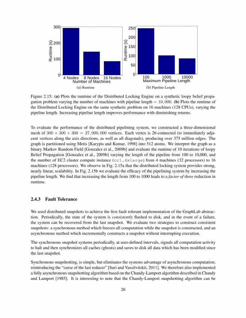
4 Nodes 8 Nodes 16 Nodes0
100
200
300
Number of Machines
Run
time
(s)
(a) Runtime
100 1000 100000
50
100
150
200
250
Maximum Pipeline Length
Run
time
(s)
(b) Pipeline Length
Figure 2.15: (a) Plots the runtime of the Distributed Locking Engine on a synthetic loopy belief propa-gation problem varying the number of machines with pipeline length = 10, 000. (b) Plots the runtime ofthe Distributed Locking Engine on the same synthetic problem on 16 machines (128 CPUs), varying thepipeline length. Increasing pipeline length improves performance with diminishing returns.
To evaluate the performance of the distributed pipelining system, we constructed a three-dimensionalmesh of 300 × 300 × 300 = 27, 000, 000 vertices. Each vertex is 26-connected (to immediately adja-cent vertices along the axis directions, as well as all diagonals), producing over 375 million edges. Thegraph is partitioned using Metis [Karypis and Kumar, 1998] into 512 atoms. We interpret the graph as abinary Markov Random Field [Gonzalez et al., 2009b] and evaluate the runtime of 10 iterations of loopyBelief Propagation [Gonzalez et al., 2009b] varying the length of the pipeline from 100 to 10,000, andthe number of EC2 cluster compute instance (cc1.4xlarge) from 4 machines (32 processors) to 16machines (128 processors). We observe in Fig. 2.15a that the distributed locking system provides strong,nearly linear, scalability. In Fig. 2.15b we evaluate the efficacy of the pipelining system by increasing thepipeline length. We find that increasing the length from 100 to 1000 leads to a factor of three reduction inruntime.
2.4.3 Fault Tolerance
We used distributed snapshots to achieve the first fault tolerant implementation of the GraphLab abstrac-tion. Periodically, the state of the system is consistently flushed to disk, and in the event of a failure,the system can be recovered from the last snapshot. We evaluate two strategies to construct consistentsnapshots: a synchronous method which freezes all computation while the snapshot is constructed, and anasynchronous method which incrementally constructs a snapshot without interrupting execution.
The synchronous snapshot systems periodically, at user-defined intervals, signals all computation activityto halt and then synchronizes all caches (ghosts) and saves to disk all data which has been modified sincethe last snapshot.
Synchronous snapshotting, is simple, but eliminates the systems advantage of asynchronous computation;reintroducing the “curse of the last reducer” [Suri and Vassilvitskii, 2011]. We therefore also implementeda fully asynchronous snapshotting algorithm based on the Chandy-Lamport algorithm described in Chandyand Lamport [1985]. It is interesting to note that the Chandy-Lamport snapshotting algorithm can be
26
implemented easily using little more than regular GraphLab update functions with the edge-consistencymodel:
Algorithm 2.11: Snapshot Update on vertex v
if v was already snapshotted thenQuit
Save Dv // Save current vertex// Save all edges connected to un-snapshotted verticesforeach u ∈ N[v] do // Loop over neighbors
if u was not snapshotted thenSave Du→v if edge u→ v existsSave Dv→u if edge v → u existsReschedule u for a Snapshot Update
Mark v as snapshotted
Theorem 2.4.1. The procedure described in Alg. 2.11 guarantees a valid serializable snapshot under thefollowing conditions:
1. Edge Consistency is used on all update functions.
2. Reschedule completes before the scope is unlocked.
3. The Snapshot Update takes priority over all other update functions.
The proof of correctness follows easily by making the following transformations and showing equivalenceto Chandy-Lamport [Chandy and Lamport, 1985].
• Vertices correspond to Machines and edges represent communication channels.
• Modifications to Dv by vertex v correspond to the machine v broadcasting the vertex data to alladjacent machines.
• Modification of either Du→v or Dv→u by vertex v corresponds to machine v sending the new datato machine u.
• The “snapshotted” flag corresponds to the marker in Chandy-Lamport.
Observe that given the conditions stated, there cannot exist a message sent from an un-snapshotted ver-tex to a snapshotted vertex. This eliminates the need for “channel recording” in the Chandy-Lamportalgorithm.
We evaluate the performance of the snapshotting algorithms on the same synthetic mesh problem de-scribed on the previous section, running on 16 machines (128 processors). We configure the implementa-tion to issue exactly one snapshot in the middle of the second iteration. In Fig. 2.16a we plot the numberof updates completed against time elapsed. The effect of the synchronous snapshot and the asynchronoussnapshot can be clearly observed: synchronous snapshots stops execution, while the asynchronous snap-shot only slows down execution. Both runs terminate at nearly the same runtime (104s for async. vs 109sfor sync.).
However, the benefits of asynchronous snapshotting become more apparent in the multi-tenancy set-ting where variation in system performance due to external load exacerbates the cost of synchronous
27
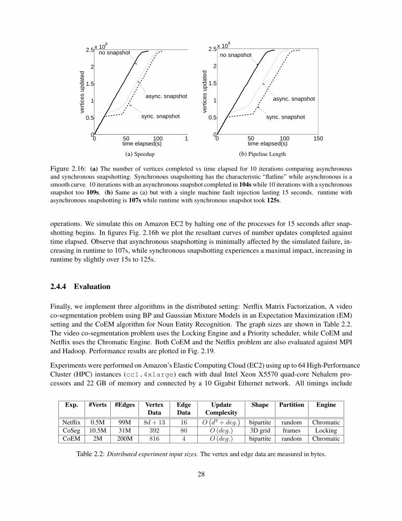
0 50 100 1500
0.5
1
1.5
2
2.5x 10⁸
time elapsed(s)
vert
ices
upd
ated
sync. snapshot
no snapshot
async. snapshot
(a) Speedup
0 50 100 1500
0.5
1
1.5
2
2.5x 10⁸
time elapsed(s)
vert
ices
upd
ated
async. snapshot
sync. snapshot
no snapshot
(b) Pipeline Length
Figure 2.16: (a) The number of vertices completed vs time elapsed for 10 iterations comparing asynchronousand synchronous snapshotting. Synchronous snapshotting has the characteristic “flatline” while asynchronous is asmooth curve. 10 iterations with an asynchronous snapshot completed in 104s while 10 iterations with a synchronoussnapshot too 109s. (b) Same as (a) but with a single machine fault injection lasting 15 seconds. runtime withasynchronous snapshotting is 107s while runtime with synchronous snapshot took 125s.
operations. We simulate this on Amazon EC2 by halting one of the processes for 15 seconds after snap-shotting begins. In figures Fig. 2.16b we plot the resultant curves of number updates completed againsttime elapsed. Observe that asynchronous snapshotting is minimally affected by the simulated failure, in-creasing in runtime to 107s, while synchronous snapshotting experiences a maximal impact, increasing inruntime by slightly over 15s to 125s.
2.4.4 Evaluation
Finally, we implement three algorithms in the distributed setting: Netflix Matrix Factorization, A videoco-segmentation problem using BP and Gaussian Mixture Models in an Expectation Maximization (EM)setting and the CoEM algorithm for Noun Entity Recognition. The graph sizes are shown in Table 2.2.The video co-segmentation problem uses the Locking Engine and a Priority scheduler, while CoEM andNetflix uses the Chromatic Engine. Both CoEM and the Netflix problem are also evaluated against MPIand Hadoop. Performance results are plotted in Fig. 2.19.
Experiments were performed on Amazon’s Elastic Computing Cloud (EC2) using up to 64 High-PerformanceCluster (HPC) instances (cc1.4xlarge) each with dual Intel Xeon X5570 quad-core Nehalem pro-cessors and 22 GB of memory and connected by a 10 Gigabit Ethernet network. All timings include
Exp. #Verts #Edges VertexData
EdgeData
UpdateComplexity
Shape Partition Engine
Netflix 0.5M 99M 8d+ 13 16 O(d3 + deg.
)bipartite random Chromatic
CoSeg 10.5M 31M 392 80 O (deg.) 3D grid frames LockingCoEM 2M 200M 816 4 O (deg.) bipartite random Chromatic
Table 2.2: Distributed experiment input sizes. The vertex and edge data are measured in bytes.
28
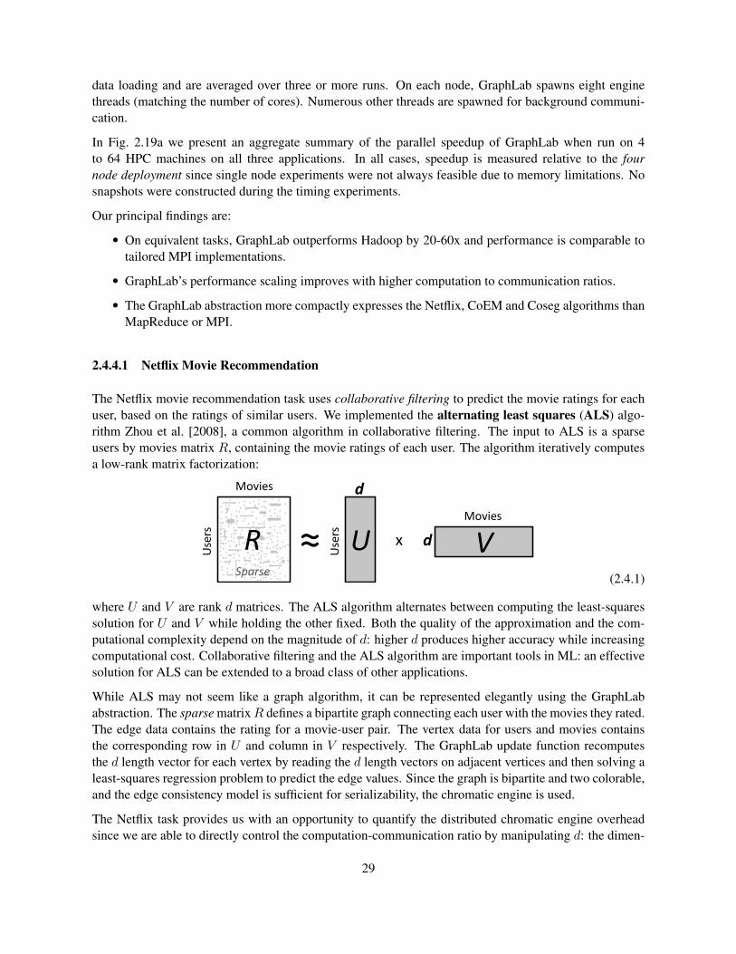
data loading and are averaged over three or more runs. On each node, GraphLab spawns eight enginethreads (matching the number of cores). Numerous other threads are spawned for background communi-cation.
In Fig. 2.19a we present an aggregate summary of the parallel speedup of GraphLab when run on 4to 64 HPC machines on all three applications. In all cases, speedup is measured relative to the fournode deployment since single node experiments were not always feasible due to memory limitations. Nosnapshots were constructed during the timing experiments.
Our principal findings are:
• On equivalent tasks, GraphLab outperforms Hadoop by 20-60x and performance is comparable totailored MPI implementations.
• GraphLab’s performance scaling improves with higher computation to communication ratios.
• The GraphLab abstraction more compactly expresses the Netflix, CoEM and Coseg algorithms thanMapReduce or MPI.
2.4.4.1 Netflix Movie Recommendation
The Netflix movie recommendation task uses collaborative filtering to predict the movie ratings for eachuser, based on the ratings of similar users. We implemented the alternating least squares (ALS) algo-rithm Zhou et al. [2008], a common algorithm in collaborative filtering. The input to ALS is a sparseusers by movies matrix R, containing the movie ratings of each user. The algorithm iteratively computesa low-rank matrix factorization:
U≈R
Movies
Use
rs
Use
rs
Sparse
d
Vx d
Movies
(2.4.1)
where U and V are rank d matrices. The ALS algorithm alternates between computing the least-squaressolution for U and V while holding the other fixed. Both the quality of the approximation and the com-putational complexity depend on the magnitude of d: higher d produces higher accuracy while increasingcomputational cost. Collaborative filtering and the ALS algorithm are important tools in ML: an effectivesolution for ALS can be extended to a broad class of other applications.
While ALS may not seem like a graph algorithm, it can be represented elegantly using the GraphLababstraction. The sparse matrixR defines a bipartite graph connecting each user with the movies they rated.The edge data contains the rating for a movie-user pair. The vertex data for users and movies containsthe corresponding row in U and column in V respectively. The GraphLab update function recomputesthe d length vector for each vertex by reading the d length vectors on adjacent vertices and then solving aleast-squares regression problem to predict the edge values. Since the graph is bipartite and two colorable,and the edge consistency model is sufficient for serializability, the chromatic engine is used.
The Netflix task provides us with an opportunity to quantify the distributed chromatic engine overheadsince we are able to directly control the computation-communication ratio by manipulating d: the dimen-
29
sionality of the approximating matrices in Eq. (2.4.1). In Fig. 2.19b we plot the speedup achieved forvarying values of d and the corresponding number of cycles required per update. Extrapolating to obtainthe theoretically optimal runtime, we estimated the overhead of Distributed GraphLab at 64 machines(512 CPUs) to be about 12x for d = 5 and about 4.9x for d = 100. Note that this overhead includes graphloading and communication. This provides us with a measurable objective for future optimizations.
Next, we compare against a Hadoop and an MPI implementation in Fig. 2.19c (d = 20 for all cases),using between 4 to 64 machines. The Hadoop implementation is part of the Mahout2 project and is widelyused. Since fault tolerance was not needed during our experiments, we reduced the Hadoop DistributedFilesystem’s (HDFS) replication factor to one. A significant amount of our effort was then spent tuningthe Hadoop job parameters to improve performance. However, even so we find that GraphLab performsbetween 40-60 times faster than Hadoop.
Performance Analysis: While some of the Hadoop inefficiency may be attributed to Java, job schedul-ing, and various design decisions, GraphLab also leads to a more efficient representation of the underlyingalgorithm. We can observe that the Map function of a Hadoop ALS implementation, performs no compu-tation and its only purpose is to emit copies of the vertex data for every edge in the graph; unnecessarilymultiplying the amount of data that need to be tracked.
For example, a user vertex that connects to 100 movies must emit the data on the user vertex 100 times,once for each movie. This results in the generation of a large amount of unnecessary network traffic andunnecessary HDFS writes. This weakness extends beyond the MapReduce abstraction, but also affectsthe graph message-passing models (such as Pregel) due to the lack of a scatter operation that would avoidsending same value multiple times to each machine. Comparatively, the GraphLab update function issimpler as users do not need to explicitly define the flow of information. Synchronization of a modifiedvertex only requires as much communication as there are ghosts of the vertex. In particular, only machinesthat require the vertex data for computation will receive it, and each machine receives each modified vertexdata at most once, even if the vertex has many neighbors.
Our MPI implementation of ALS is highly optimized, and uses synchronous MPI collective operations forcommunication. The computation is broken into super-steps that alternate between recomputing the latentuser and movies low rank matrices. Between super-steps the new user and movie values are scattered(using MPI Alltoall) to the machines that need them in the next super-step. As a consequence our MPIimplementation of ALS is roughly equivalent to an optimized Pregel version of ALS with added supportfor parallel broadcasts. Surprisingly, GraphLab was able to outperform the MPI implementation. Weattribute the performance to the use of background asynchronous communication in GraphLab.
Finally, we can evaluate the effect of enabling dynamic computation. In Fig. 2.17, we plot the test errorobtained over time using a dynamic update schedule as compared to a static BSP-style update schedule.This dynamic schedule is easily represented in GraphLab while it is difficult to express using Pregelmessaging semantics. We observe that a dynamic schedule converges much faster, reaching a low testerror in about half amount of work.
2https://issues.apache.org/jira/browse/MAHOUT-542
30
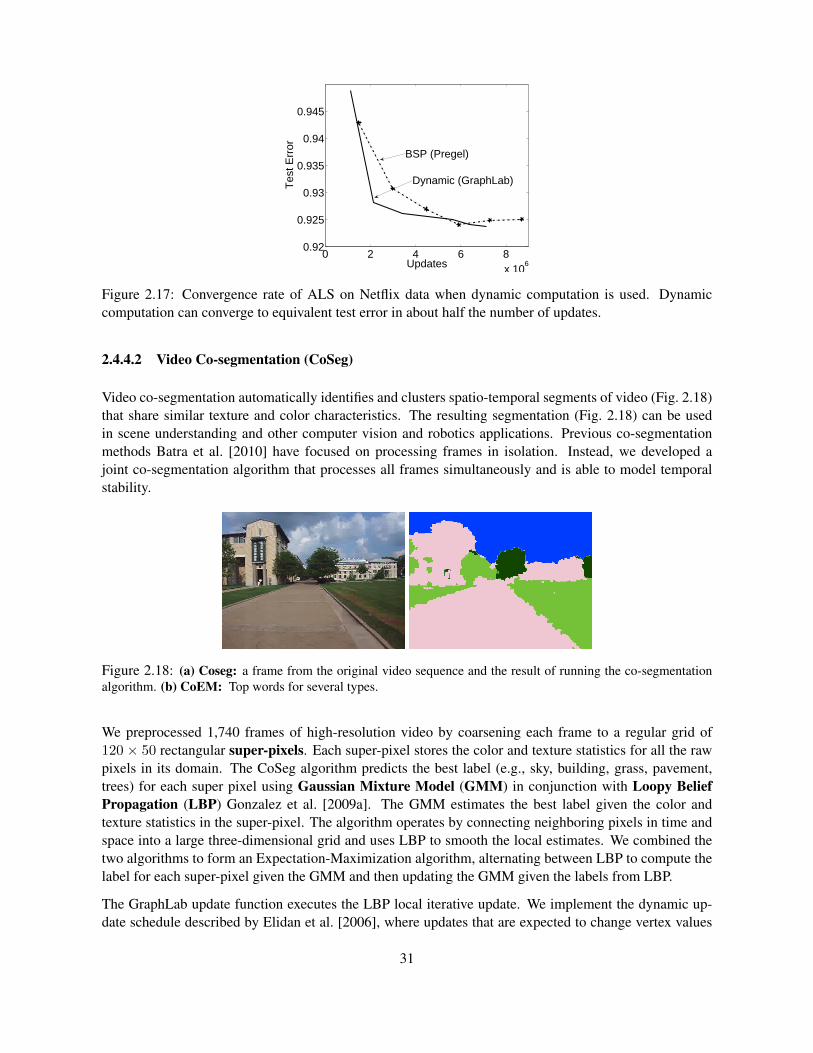
0 2 4 6 8x 10
6
0.92
0.925
0.93
0.935
0.94
0.945
Updates
Tes
t Err
or
BSP (Pregel)
Dynamic (GraphLab)
Figure 2.17: Convergence rate of ALS on Netflix data when dynamic computation is used. Dynamiccomputation can converge to equivalent test error in about half the number of updates.
2.4.4.2 Video Co-segmentation (CoSeg)
Video co-segmentation automatically identifies and clusters spatio-temporal segments of video (Fig. 2.18)that share similar texture and color characteristics. The resulting segmentation (Fig. 2.18) can be usedin scene understanding and other computer vision and robotics applications. Previous co-segmentationmethods Batra et al. [2010] have focused on processing frames in isolation. Instead, we developed ajoint co-segmentation algorithm that processes all frames simultaneously and is able to model temporalstability.
Figure 2.18: (a) Coseg: a frame from the original video sequence and the result of running the co-segmentationalgorithm. (b) CoEM: Top words for several types.
We preprocessed 1,740 frames of high-resolution video by coarsening each frame to a regular grid of120 × 50 rectangular super-pixels. Each super-pixel stores the color and texture statistics for all the rawpixels in its domain. The CoSeg algorithm predicts the best label (e.g., sky, building, grass, pavement,trees) for each super pixel using Gaussian Mixture Model (GMM) in conjunction with Loopy BeliefPropagation (LBP) Gonzalez et al. [2009a]. The GMM estimates the best label given the color andtexture statistics in the super-pixel. The algorithm operates by connecting neighboring pixels in time andspace into a large three-dimensional grid and uses LBP to smooth the local estimates. We combined thetwo algorithms to form an Expectation-Maximization algorithm, alternating between LBP to compute thelabel for each super-pixel given the GMM and then updating the GMM given the labels from LBP.
The GraphLab update function executes the LBP local iterative update. We implement the dynamic up-date schedule described by Elidan et al. [2006], where updates that are expected to change vertex values
31
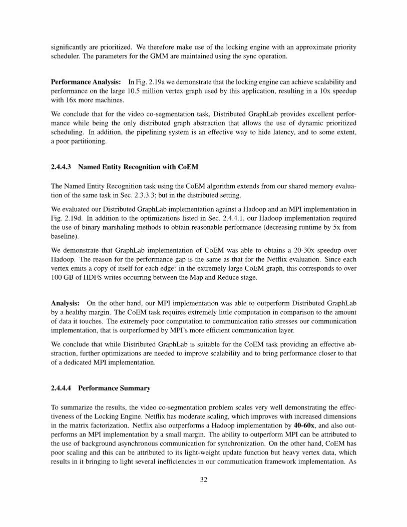
significantly are prioritized. We therefore make use of the locking engine with an approximate priorityscheduler. The parameters for the GMM are maintained using the sync operation.
Performance Analysis: In Fig. 2.19a we demonstrate that the locking engine can achieve scalability andperformance on the large 10.5 million vertex graph used by this application, resulting in a 10x speedupwith 16x more machines.
We conclude that for the video co-segmentation task, Distributed GraphLab provides excellent perfor-mance while being the only distributed graph abstraction that allows the use of dynamic prioritizedscheduling. In addition, the pipelining system is an effective way to hide latency, and to some extent,a poor partitioning.
2.4.4.3 Named Entity Recognition with CoEM
The Named Entity Recognition task using the CoEM algorithm extends from our shared memory evalua-tion of the same task in Sec. 2.3.3.3; but in the distributed setting.
We evaluated our Distributed GraphLab implementation against a Hadoop and an MPI implementation inFig. 2.19d. In addition to the optimizations listed in Sec. 2.4.4.1, our Hadoop implementation requiredthe use of binary marshaling methods to obtain reasonable performance (decreasing runtime by 5x frombaseline).
We demonstrate that GraphLab implementation of CoEM was able to obtains a 20-30x speedup overHadoop. The reason for the performance gap is the same as that for the Netflix evaluation. Since eachvertex emits a copy of itself for each edge: in the extremely large CoEM graph, this corresponds to over100 GB of HDFS writes occurring between the Map and Reduce stage.
Analysis: On the other hand, our MPI implementation was able to outperform Distributed GraphLabby a healthy margin. The CoEM task requires extremely little computation in comparison to the amountof data it touches. The extremely poor computation to communication ratio stresses our communicationimplementation, that is outperformed by MPI’s more efficient communication layer.
We conclude that while Distributed GraphLab is suitable for the CoEM task providing an effective ab-straction, further optimizations are needed to improve scalability and to bring performance closer to thatof a dedicated MPI implementation.
2.4.4.4 Performance Summary
To summarize the results, the video co-segmentation problem scales very well demonstrating the effec-tiveness of the Locking Engine. Netflix has moderate scaling, which improves with increased dimensionsin the matrix factorization. Netflix also outperforms a Hadoop implementation by 40-60x, and also out-performs an MPI implementation by a small margin. The ability to outperform MPI can be attributed tothe use of background asynchronous communication for synchronization. On the other hand, CoEM haspoor scaling and this can be attributed to its light-weight update function but heavy vertex data, whichresults in it bringing to light several inefficiencies in our communication framework implementation. As
32
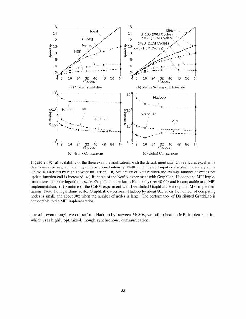
4 8 16 24 32 40 48 56 6412
4
6
8
10
12
14
16
#Nodes
Spe
edup
Ideal
CoSeg
Netflix
NER
(a) Overall Scalability
4 8 16 24 32 40 48 56 6412
4
6
8
10
12
14
16
#Nodes
Spe
edup
Ideald=100 (30M Cycles)d=50 (7.7M Cycles)
d=20 (2.1M Cycles)d=5 (1.0M Cycles)
(b) Netflix Scaling with Intensity
4 8 16 24 32 40 48 56 6410
1
102
103
104
#Nodes
Run
time(
s) Hadoop MPI
GraphLab
(c) Netflix Comparisons
4 8 16 24 32 40 48 56 6410
1
102
103
104
#Nodes
Run
time(
s)
Hadoop
GraphLab
MPI
(d) CoEM Comparisons
Figure 2.19: (a) Scalability of the three example applications with the default input size. CoSeg scales excellentlydue to very sparse graph and high computational intensity. Netflix with default input size scales moderately whileCoEM is hindered by high network utilization. (b) Scalability of Netflix when the average number of cycles perupdate function call is increased. (c) Runtime of the Netflix experiment with GraphLab, Hadoop and MPI imple-mentations. Note the logarithmic scale. GraphLab outperforms Hadoop by over 40-60x and is comparable to an MPIimplementation. (d) Runtime of the CoEM experiment with Distributed GraphLab, Hadoop and MPI implemen-tations. Note the logarithmic scale. GraphLab outperforms Hadoop by about 80x when the number of computingnodes is small, and about 30x when the number of nodes is large. The performance of Distributed GraphLab iscomparable to the MPI implementation.
a result, even though we outperform Hadoop by between 30-80x, we fail to beat an MPI implementationwhich uses highly optimized, though synchronous, communication.
33
2.5 Conclusion
The GraphLab 1 abstraction is easy to implement in the shared memory setting requiring little morethan standard datastructures and parallel primitives. The distributed implementation however, requires asubstantially larger effort since we must address issues of graph placement, data consistency and faulttolerance.
Our key contributions are:
• The GraphLab 1 abstraction comprising of:
A data graph which represents the data and computational dependencies.
Update functions which describe local computation
A Sync mechanism for aggregating global state.
A data consistency model which determines the extent to which computation can overlap.
• Shared Memory Implementation:
A shared memory implementation of the GraphLab 1 abstraction.
A collection of concurrent schedulers which allow for dynamic, prioritized computation.
Experimental evaluations of parameter learning and inference in graphical models, Gibbs sam-pling, CoEM, Lasso and compressed sensing on real-world problems.
• Distributed Implementation:
A distributed data graph format built around a two-stage partitioning scheme which allowsfor efficient load balancing and distributed ingress on variable-sized cluster deployments.
Two GraphLab 1 engines:
− A chromatic engine that is partially synchronous and assumes the existence of a graphcoloring, and
− a locking engine that is fully asynchronous, supports general graph structures, and reliesupon a graph-based pipelined locking system to hide network latency.
An asynchronous snapshot algorithm based on Chandy-Lamport snapshots that can be ex-pressed using regular GraphLab 1 primitives.
Evaluation of the distributed implementation on three challenging Machine Learning tasks ofCoEM, ALS, and Video Cosegmentation.
The resultant system is highly expressive and easy to use, and permits a rather broad range of algorithmsto be developed, and parallelized, with relatively little effort. Danny Bickson has developed, and releasedas open source, a large number of different matrix factorization libraries implemented in GraphLab 1.Furthermore, the shared memory GraphLab 1 implementation has been instrumental in the developmentof some new graphical model inference procedures such as parallel Gibbs Samplers [Gonzalez et al.,2011], and kernelized belief propagation [Song et al., 2011].
34
Chapter 3
PowerGraph
Restricting the Abstraction for Performance
In the previous chapter, we defined the GraphLab 1 abstraction which defined the notion of graph compu-tation and described both a shared memory and a distributed memory implementation of the abstraction.In this chapter, we begin by describing the lessons learned through the development of GraphLab 1 andexplore the limitations of the model. We then design the PowerGraph abstraction [Gonzalez et al., 2012]which addresses the fundamental performance limitations of GraphLab 1, allowing our implementation toachieve the next order of magnitude gain in both performance and scalability.
We begin in Sec. 3.1 by enumerating the limitations of GraphLab 1 which block scalability, follow-ing which in Sec. 3.2 we describe the Gather-Apply-Scatter model which we can use to analyze bothGraphLab 1 and Pregel in a common framework.
Next, in Sec. 3.3, we describe the PowerGraph abstraction which factorizes the GraphLab 1 update func-tion into the Gather, Apply and Scatter phases. The new abstraction also permits the use of the vertex-separator model of distributed graph placement, bringing about large reductions in communication andstorage requirements (Sec. 3.4). We also introduce streaming graph partitioning heuristics to reduce com-munication requirements, while ensuring load balancing. Finally, in Sec. 3.6 we describe a distributedimplementation of the PowerGraph abstraction, and demonstrate that we are able to achieve large per-formance gains, achieving state of the art performance, and outperforming published results on somebenchmarks.
3.1 GraphLab 1 Limitations
Through the design, implementation and development of a shared memory and distributed version of theGraphLab 1 abstraction in the previous chapter, we were made aware of some problems and limitations ofthe abstraction; and what is needed to scale GraphLab to even larger problems.
35
(a) Twitter In-Degree (b) Twitter Out-Degree
Figure 3.1: The in and out degree distributions of the Twitter follower network plotted in log-log scale.
3.1.1 Gather vs Scatter
GraphLab 1 has very efficient scatter capability, where a modification of a single vertex, can be efficientlytransmitted to all machines which need it, with no unnecessary replication of data. Pregel however, re-quires excessive replication of data, requiring modifications of vertex data to be communicated #degreetimes (Sec. 2.4.4.1).
On the other hand, Pregel [Malewicz et al., 2010] has very efficient gather capability which allows in-formation going to the same vertex to be “pre-combined”, reducing network communication. GraphLab1 however, requires the update function to have full access to the entire scope and not just an aggre-gated value. As a result, even though an aggregated value might be sufficient, GraphLab 1 will performexcessive unnecessary communication.
GraphLab 1 will need fundamental changes to the abstraction to be able to efficiently express both gather-like operations and scatter-like operations.
3.1.2 Natural Graphs
One of the hallmark properties of natural graphs is their skewed power-law degree distribution [Faloutsoset al., 1999]: most vertices have relatively few neighbors while a few have many neighbors (e.g., celebritiesin a social network). Under a power-law degree distribution the probability that a vertex has degree d isgiven by:
P (d) ∝ d−α, (3.1.1)
where the exponent α is a positive constant that controls the “skewness” of the degree distribution. Higherα implies that the graph has lower density (ratio of edges to vertices), and that the vast majority of verticesare low degree. As α decreases, the graph density and number of high degree vertices increases. Mostnatural graphs typically have a power-law constant around α ≈ 2. For example, Faloutsos et al. [1999]estimated that the inter-domain graph of the Internet has a power-law constant α ≈ 2.2. One can visualizethe skewed power-law degree distribution by plotting the number of vertices with a given degree in log-logscale. In Fig. 3.1, we plot the in and out degree distributions of the Twitter follower network demonstratingthe characteristic linear power-law form.
36
Examining the behavior of the distributed GraphLab 1 implementation on natural graphs demonstratedseveral fundamental limitations of the GraphLab 1 abstraction.
Engine Performance The good performance of GraphLab 1’s locking engine on regular graphs in theearlier sections is tarnished by its poor performance on power-law graphs. We demonstrate this by gener-ating a domain graph from the Yahoo! Web Graph [Yahoo, Retrieved 2011] producing a power law graphwith 25.5M vertices and 355M, as well as a 26-connected 300 × 300 × 300 grid graph with 27, 000, 000vertices and 375 million edges (the same synthetic graph evaluated in Sec. 2.4.2.2). The performanceresults of running 2 iterations of loopy belief propagation on this graph is shown in Fig. 3.2. We observefrom Fig. 3.2c that speedup is extremely poor, providing almost no speedup at all as number of machinesis increased. To put runtime in perspective we observe that GraphLab 1 took nearly 500s per iterationusing 16 machines, while a regular graph with of the same size took only 10s per iteration. In otherwords, a mere change in connectivity structure can result in 50x decrease in performance even though thetotal amount of work is held constant.
Excessive Memory Load Loading the entire AltaVista Web Graph of 1.4B vertices and 6.6B edgesinto memory for PageRank computation on 64 machines required over 51GB of memory per machinefor a total memory load of over 3 terabytes, far exceeding the real size of the graph. This is due to thepoor partitioning scheme (random partitioning was used), which resulted in an excessive number of ghostvertices and replicated edges. Performance suffers as a result of excessive communication.
3.1.2.1 Challenges Of Natural Graphs
Natural graphs presents a challenge not just to GraphLab 1, but is also a fundamental limitation to allgraph-parallel abstractions such as GraphLab 1 and Pregel. To minimize communication requirementsand memory load, distributed graph systems rely on the availability of a good graph partitioning.
Where the graph is G = (V,E), a graph bi-partitioning is a partition of the set of vertices V into ap-proximately balanced two disjoint sets B and B′ such that the number of edges crossing the partition isminimized. Formally:
B,B′ = arg minB,B′
∣∣(i, j) ∈ E s.t. i ∈ B, j ∈ B′∣∣
subj. to B ∪B′ = V and B ∩B′ = ∅ andmax(|B|, |B′)|V |/2
≤ γ
where γ is a balance tolerance parameter. Observe that if γ = 1, the partitions must be exactly bal-anced, while γ > 1 permits some slackness. The objective can be analogously generalized to k-waypartitions.
Mesh-like graph structures are relatively easily to partition and heuristic partitioners such as Metis orParMetis [Karypis and Kumar, 1998] provide good results in very little runtime. Power law graphs how-ever, are known empirically to have poor graph partitions [Lang, 2004, Leskovec et al., 2008b]. We havealso empirically discovered that many heuristic graph partitioners (Metis [Karypis and Kumar, 1998],
37
4 Nodes 8 Nodes 16 Nodes0
100
200
300
Number of Machines
Run
time
(s)
(a) Regular Graph Runtime
100 1000 100000
50
100
150
200
250
Maximum Pipeline Length
Run
time
(s)
(b) Regular Graph Varying Pipeline Length
4 Nodes 8 Nodes 16 Nodes0
200
400
600
800
1000
Number of Machines
Run
time
(s)
(c) Power Law Graph Runtime
10K 100K 1M0
500
1000
1500
Maximum Pipeline Length
Run
time
(s)
(d) Power Law Graph Varying Pipeline Length
Figure 3.2: (a) Plots the runtime of the Distributed Locking Engine on 10 iterations of a loopy belief propagationproblem on a regular graph varying the number of machines. Pipeline length was set to 10,000. Nearly linearspeedup was observed. (b) Plots the runtime of the Distributed Locking Engine on the same synthetic problemon 16 machines (128 CPUs), varying the length of the pipeline. Increased pipeline length results in improvedperformance, but with diminishing returns. (c) Plots the runtime of the Distributed Locking Engine on 2 iterationsof loopy belief propagation on a domain graph derived from the Yahoo Web Graph varying the number of machines.Pipeline length was set to 1M. Negligible Speedup is observed. (d) Plots the runtime of the Distributed LockingEngine on the same problem on 16 machines (128 CPUs), varying the length of the pipeline. Increased pipelinelength results in slightly improved performance.
Scotch [Chevalier and Pellegrini, 2006] and Zoltan[Devine et al., 2006] as of 2010) do not behave wellunder Power Law graph structures; either crashing, or running out of memory1.
Both GraphLab 1 and Pregel depend on graph partitioning to minimize communication and ensure workbalance. However, in the case of natural graphs both are forced to resort to hash-based (random) partition-ing which has extremely poor locality.
This has the following implications:
1Most graph partitioning libraries use a coarsening procedure to collapse the size of the graph. However, in power lawgraphs, the coarsening procedure does not effectively decrease the number of edges in the graph [Abou-Rjeili and Karypis,2006], resulting in high runtimes and memory consumption even on relatively small graphs. Coarsening heuristics that are morewell-behaved exist for power-law graphs [Abou-Rjeili and Karypis, 2006], but we were unable to locate an implementation ofsuch procedures as of our evaluation in 2010
38
Computation: While multiple vertex-programs may execute in parallel, existing graph-parallel abstrac-tions do not parallelize within individual vertex-programs. A vertex program which has complexity linearin the number of edges will thus encounter scalability and performance issues which are exacerbated bypoor partitioning quality.
Work Balance: The power-law degree distribution can lead to substantial work imbalance in graph par-allel abstractions that treat vertices symmetrically. Since the storage, communication, and computationcomplexity of the vertex-program may be linear in the degree, the running time of vertex-programs canvary widely [Suri and Vassilvitskii, 2011].
Communication: The skewed degree distribution of natural-graphs leads to communication asymmetryand consequently bottlenecks. In addition, high-degree vertices can force messaging abstractions, such asPregel, to generate and send many identical messages.
Storage: Since graph parallel abstractions must locally store the adjacency information for each vertex,each vertex requires memory linear in its degree. Consequently, high-degree vertices can exceed thememory capacity of a single machine.
3.1.3 Serializability Frequently Unnecessary
Serializability is a useful property to have for the reasons described in Sec. 1.1.1. While many Ma-chine Learning algorithms require serializability for various theoretical guarantees to hold, empiricallyit has been observed for many algorithms, that serializability is not strictly necessary. In particular,serializability-breaking parallel/distributed implementations of various algorithms (LDA [Smola and Narayana-murthy, 2010], BP [Gonzalez et al., 2009a] and Matrix Factorization) have been empirically demonstratedto converge well.
Breaking serializability breaks theoretical guarantees of many algorithms, but provide large gains inthroughput. This is most significant in the distributed setting since we avoid the cost of distributed lock-ing. On the other hand, it has been demonstrated both empirically and theoretically that some algorithmshave limits on non-serializable parallelism [Bradley et al., 2011, Recht et al., 2011, Siapas, 1996], eitherconverging slower, or failing to converge when there is a large amount of parallelism. Therefore, it isstill desirable to provide an abstraction with a broad set of consistency rules, allowing serializability to bebroken when unnecessary, but providing it when required.
3.2 Characterization
While the implementation of ML vertex-programs in GraphLab 1 and Pregel differ in how they collect anddisseminate information, they share a common overall structure. To characterize this common structureand differentiate between vertex and edge specific computation we introduce the GAS model of graphcomputation.
The GAS model represents three conceptual phases of a vertex-program: Gather, Apply, and Scatter. Inthe gather phase, information about adjacent vertices and edges is collected through a generalized sumover the neighborhood of the vertex u on which Q(u) is run:
Σ←⊕
v∈N[u]
g (Du, Du−v, Dv) . (3.2.1)
39
where Du, Dv, and Du−v are the values (program state and meta-data) for vertices u and v and edge(u, v). The user defined sum ⊕ operation must be commutative and associative and can range from anumerical sum to the union of the data on all neighboring vertices and edges.
The resulting value Σ is used in the apply phase to update the value of the central vertex:
Dnewu ← a (Du,Σ) . (3.2.2)
Finally the scatter phase uses the new value of the central vertex to update the data on adjacent edges:
∀v ∈ N[u] : (Du−v)← s (Dnewu , Du−v, Dv) . (3.2.3)
The fan-in and fan-out of a vertex-program is determined by the corresponding gather and scatter phases.For instance, in PageRank, the gather phase only operates on in-edges and the scatter phase only operateson out-edges. However, for many ML algorithms the graph edges encode ostensibly symmetric relation-ships, like friendship, in which both the gather and scatter phases touch all edges. In this case the fan-inand fan-out are equal. As we will show in Sec. 3.1.2.1, the ability for graph parallel abstractions to supportboth high fan-in and fan-out computation is critical for efficient computation on natural graphs.
GraphLab 1 and Pregel express GAS programs in very different ways. In the Pregel abstraction the gatherphase is implemented using message combiners and the apply and scatter phases are expressed in thevertex program. Conversely, GraphLab 1 exposes the entire neighborhood to the vertex-program andallows the user to define the gather and apply phases within their program. The GraphLab 1 abstractionimplicitly defines the communication aspects of the gather/scatter phases by ensuring that changes madeto the vertex or edge data are automatically visible to adjacent vertices. It is also important to note thatGraphLab 1 does not differentiate between edge directions.
3.3 PowerGraph Abstraction
To address the challenges of computation on power-law graphs, we introduce PowerGraph [Gonzalezet al., 2012], a new graph-parallel abstraction that eliminates the degree dependence of the vertex-programby directly exploiting the GAS decomposition to factor vertex-programs over edges. By lifting the Gatherand Scatter phases into the abstraction, PowerGraph is able to retain the natural “think-like-a-vertex”philosophy [Malewicz et al., 2010] while distributing the computation of a single vertex-program over theentire cluster.
PowerGraph combines the best features from both Pregel and GraphLab 1. From GraphLab 1, Power-Graph borrows the data-graph and shared-memory view of computation eliminating the need for users toarchitect the movement of information. From Pregel, PowerGraph borrows the commutative, associativegather concept. PowerGraph supports both the highly-parallel bulk-synchronous Pregel model of compu-tation as well as the computationally efficient asynchronous GraphLab 1 model of computation.
Like GraphLab 1, the state of a PowerGraph program factors according to a data-graph with user definedvertex data Dv and edge data Du→v. Just like the GraphLab 1 abstraction, the PowerGraph abstractiondoes not place special meaning on the edge direction but treats it simply as a property of the edge. Wewill therefore frequently use Du−v to refer to the contents of an edge u− v when the direction of the edgeis unimportant.
40
interface GASVertexProgram(u) {// Run on gather_nbrs(u)
gather(Du, Du−v, Dv) → Accumsum(Accum left, Accum right) → Accumapply(Du,Accum) → Dnew
u
// Run on scatter_nbrs(u)
scatter(Dnewu ,Du−v,Dv) → (Dnew
u−v, Accum)}
Figure 3.3: All PowerGraph programs must implement the stateless gather, sum, apply, and scatter functions.
Algorithm 3.1: Vertex-Program Execution SemanticsInput: Center vertex uif Cache Disabled then
// Basic Gather-Apply-Scatter Modelforeach neighbor v in gather nbrs(u) do
au ← sum(au, gather(Du, Du−v , Dv))
Du ← apply(Du, au)foreach neighbor v scatter nbrs(u) do
(Du−v)← scatter(Du, Du−v , Dv)
else if Cache Enabled then// Faster GAS Model with Delta Cachingif cached accumulator au is empty then
foreach neighbor v in gather nbrs(u) doau ← sum(au, gather(Du, Du−v , Dv))
Du ← apply(Du, au)foreach neighbor v scatter nbrs(u) do
(Du−v,∆a)← scatter(Du, Du−v , Dv)if av and ∆a are not Empty then av ← sum(av , ∆a)else av ← Empty
The data stored in the data-graph includes both meta-data (e.g., urls and edge weights) as well as com-putation state (e.g., the PageRank of vertices). In Sec. 3.4 we introduce vertex-cuts which allow Power-Graph to efficiently represent and store power-law graphs in a distributed environment. We now describethe PowerGraph abstraction and how it can be used to naturally decompose vertex-programs. Then inSec. 3.4 through Sec. 3.6 we discuss how to implement the PowerGraph abstraction in a distributed envi-ronment.
3.3.1 GAS Vertex-Programs
Computation in the PowerGraph abstraction is encoded as a state-less vertex-program which implementsthe GASVertexProgram interface (Fig. 3.3) and therefore explicitly factors into the gather, sum, apply,and scatter functions. Each function is invoked in stages by the PowerGraph engine following the seman-tics in Alg. 3.1. By factoring the vertex-program, the PowerGraph execution engine can distribute a singlevertex-program over multiple machines and move computation to the data.
41

// gather_nbrs: IN_NBRS
gather(Du, Du−v, Dv):return Dv.rank/outdeg(v)
sum(a, b): return a + bapply(Du, acc):
rnew = 0.15 + 0.85 * accDu.delta = rnew - Du.rankDu.rank = rnew
// scatter_nbrs: OUT_NBRS
scatter(Du,Du−v,Dv):if(|Du.delta|>ε)
Activate(v)
(a) PageRank
// gather_nbrs: ALL_NBRS
gather(Du, Du−v, Dv):return set(Dv)
sum(a, b):return union(a, b)
apply(Du, S):Du = min c where c /∈ S
// scatter_nbrs: ALL_NBRS
scatter(Du,Du−v,Dv):// Nbr changed since gather
if(Du == Dv)Activate(v)
(b) Greedy Graph Coloring
// gather_nbrs: ALL_NBRS
gather(Du, Du−v, Dv):return Dv + Dv−u
sum(a, b):return min(a, b)
apply(Du, new_dist):Du = new_dist
// scatter_nbrs: ALL_NBRS
scatter(Du,Du−v,Dv):// If changed activate nbr
if(changed(Du))Activate(v)
(c) Single Source Shortest Path (SSSP)
Figure 3.4: The PageRank, graph-coloring, and single source shortest path algorithms implemented in the basicPowerGraph abstraction without Delta Caching.
During the gather phase the gather and sum functions are used as a map and reduce to collect infor-mation about the neighborhood of the vertex. The gather function is invoked in parallel on the edgesadjacent to u. The particular set of edges is determined by gather nbrs which can be none, in, out,or all. The gather function is passed the data on the adjacent vertex and edge and returns a temporaryaccumulator (a user defined type). The result is combined using the commutative and associative sumoperation. The final result au of the gather phase is passed to the apply phase and cached by Power-Graph.
After the gather phase has completed, the apply function takes the final accumulator and computes anew vertex value Du which is atomically written back to the graph. The size of the accumulator au andcomplexity of the apply function play a central role in determining the network and storage efficiency ofthe PowerGraph abstraction and should be sub-linear and ideally constant in the degree.
During the scatter phase, the scatter function is invoked in parallel on the edges adjacent to u pro-ducing new edge values Du−v which are written back to the data-graph. As with the gather phase, thescatter nbrs determines the particular set of edges on which scatter is invoked. The scatter func-tion returns an optional value ∆a which is used to dynamically update the cached accumulator av for theadjacent vertex (see Sec. 3.3.2).
In Fig. 3.4 we implement the PageRank, greedy graph coloring, and single source shortest path algorithmsusing the PowerGraph abstraction. In PageRank the gather and sum functions collect the total value ofthe adjacent vertices, the apply function computes the new PageRank, and the scatter function is used toactivate adjacent vertex-programs if necessary. In graph coloring the gather and sum functions collectthe set of colors on adjacent vertices, the apply function computes a new color, and the scatter functionactivates adjacent vertices if they violate the coloring constraint. Finally in single source shortest path(SSSP), the gather and sum functions compute the shortest path through each of the neighbors, the applyfunction returns the new distance, and the scatter function activates affected neighbors.
42

// gather_nbrs: IN_NBRS
gather(Du, Du−v, Dv):return Dv.rank / outdeg(v)
sum(a, b): return a + bapply(Du, acc):
rnew = 0.15 + 0.85 * accDu.delta = rnew - Du.rankDu.rank = rnew
// scatter_nbrs: OUT_NBRS
scatter(Du,Du−v,Dv):if(|Du.delta|>ε)
Activate(v)return Du.delta / outdeg(u)
(a) PageRank With Delta Caching
// gather_nbrs: ALL_NBRS
gather(Du, Du−v, Dv):return Dv + Dv−u
sum(a, b):return min(a, b)
apply(Du, new_dist):Du = new_dist
// scatter_nbrs: ALL_NBRS
scatter(Du,Du−v,Dv):// If changed activate nbr
if(changed(Du))Activate(v)
return Du + Du−v
(b) SSSP with Delta Caching
Figure 3.5: The PageRank, and single source shortest path algorithms implemented in the PowerGraph abstractionand taking advantage of Delta Caching.
3.3.2 Delta Caching
In many cases a vertex-program will be triggered in response to a change in a few of its neighbors. Thegather operation is then repeatedly invoked on all neighbors, many of which remain unchanged, therebywasting computation cycles. For many algorithms [Ahmed et al., 2012] it is possible to dynamicallymaintain the result of the gather phase au and skip the gather on subsequent iterations.
The PowerGraph engine maintains a cache of the accumulator au from the previous gather phase foreach vertex. The scatter function can optionally return an additional ∆a which is atomically added tothe cached accumulator av of the neighboring vertex v using the sum function. If ∆a is not returned,then the neighbor’s cached av is cleared, forcing a complete gather on the subsequent execution of thevertex-program on the vertex v. When executing the vertex-program on v the PowerGraph engine usesthe cached av if available, bypassing the gather phase.
Intuitively, ∆a acts as an additive correction on-top of the previous gather for that edge. More formally, ifthe accumulator type forms an abelian group: has a commutative and associative sum (+) and an inverse(−) operation, then we can define
∆a = gather(Du, Dnewu−v, D
newv )− gather(Du, Du−v, Dv). (3.3.1)
We demonstrate Delta Caching by modify the PageRank and the SSSP algorithms in Fig. 3.5. In thePageRank example (Fig. 3.4) we take advantage of the abelian nature of the PageRank sum operation.In the SSSP example, while the min operation is not abelian, the nature of the computation ensures thatthe distance value on each vertex is always decreasing, thus allowing the delta cache to be updated cor-rectly.
3.3.3 Scheduling
PowerGraph continues to inherit the dynamic scheduling capability of GraphLab 1. The PowerGraphengine maintains a set of active vertices on which to eventually execute the vertex-program. The user
43
initiates computation by calling Activate(v) or Activate all(). The PowerGraph engine thenproceeds to execute the vertex-program on the active vertices until none remain. Once a vertex-programcompletes the scatter phase it becomes inactive until it is reactivated.
Vertices can activate themselves and neighboring vertices. Each function in a vertex-program can onlyactivate vertices visible in the arguments to that function. For example the scatter function invoked on theedge (u, v) can only activate the vertices u and v. This restriction is essential to ensure that activationevents are generated on machines on which they can be efficiently processed.
The order in which activated vertices are executed is up to the PowerGraph execution engine. The onlyguarantee is that all activated vertices are eventually executed. This flexibility in scheduling enablesPowerGraph programs to be executed both synchronously and asynchronously, leading to different trade-offs in algorithm performance, system performance, and determinism.
3.3.3.1 Bulk Synchronous Execution
When run synchronously, the PowerGraph engine executes the gather, apply, and scatter phases in order.Each phase, called a minor-step, is run synchronously on all active vertices with a barrier at the end. Wedefine a super-step as a complete series of GAS minor-steps. Changes made to the vertex data and edgedata are committed at the end of each minor-step and are visible in the subsequent minor-step. Verticesactivated in each super-step are executed in the subsequent super-step.
The synchronous execution model ensures a deterministic execution regardless of the number of machinesand closely resembles Pregel. However, the frequent barriers and inability to operate on the most recentdata can lead to an inefficient distributed execution and slow algorithm convergence. To address theselimitations PowerGraph also supports asynchronous execution.
3.3.3.2 Asynchronous Execution
When run asynchronously, the PowerGraph engine executes active vertices as processor and networkresources become available. Changes made to the vertex and edge data during the apply and scatterfunctions are immediately committed to the graph and visible to subsequent computation on neighboringvertices.
By using processor and network resources as they become available and making any changes to the data-graph immediately visible to future computation, an asynchronous execution can more effectively utilizeresources and accelerate the convergence of the underlying algorithm. For example, the greedy graph-coloring algorithm in Fig. 3.4 will not converge when executed synchronously but converges quicklywhen executed asynchronously. The merits of asynchronous computation have been studied extensivelyin the context of numerical algorithms [Bertsekas and Tsitsiklis, 1989]. In Gonzalez et al. [2009a,b], Lowet al. [2012] we demonstrated that asynchronous computation can lead to both theoretical and empiricalgains in algorithm and system performance.
Unfortunately, the behavior of the asynchronous execution depends on the number machines and availabil-ity of network resources leading to non-determinism that can complicate algorithm design and debugging.Furthermore, for some algorithms, like statistical simulation, the resulting non-determinism, if not care-fully controlled, can lead to instability or even divergence [Gonzalez et al., 2011].
44
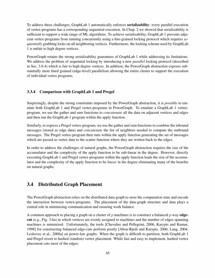
To address these challenges, GraphLab 1 automatically enforces serializability: every parallel executionof vertex-programs has a corresponding sequential execution. In Chap. 2 we showed that serializability issufficient to support a wide range of ML algorithms. To achieve serializability, GraphLab 1 prevents adja-cent vertex-programs from running concurrently using a fine-grained locking protocol which requires se-quentially grabbing locks on all neighboring vertices. Furthermore, the locking scheme used by GraphLab1 is unfair to high degree vertices.
PowerGraph retains the strong serializability guarantees of GraphLab 1 while addressing its limitations.We address the problem of sequential locking by introducing a new parallel locking protocol (describedin Sec. 3.6.4) which is fair to high degree vertices. In addition, the PowerGraph abstraction exposes sub-stantially more fined grained (edge-level) parallelism allowing the entire cluster to support the executionof individual vertex programs.
3.3.4 Comparison with GraphLab 1 and Pregel
Surprisingly, despite the strong constraints imposed by the PowerGraph abstraction, it is possible to em-ulate both GraphLab 1 and Pregel vertex-programs in PowerGraph. To emulate a GraphLab 1 vertex-program, we use the gather and sum functions to concatenate all the data on adjacent vertices and edgesand then run the GraphLab 1 program within the apply function.
Similarly, to express a Pregel vertex-program, we use the gather and sum functions to combine the inboundmessages (stored as edge data) and concatenate the list of neighbors needed to compute the outboundmessages. The Pregel vertex-program then runs within the apply function generating the set of messageswhich are passed as vertex data to the scatter function where they are written back to the edges.
In order to address the challenges of natural graphs, the PowerGraph abstraction requires the size of theaccumulator and the complexity of the apply function to be sub-linear in the degree. However, directlyexecuting GraphLab 1 and Pregel vertex-programs within the apply function leads the size of the accumu-lator and the complexity of the apply function to be linear in the degree eliminating many of the benefitson natural graphs.
3.4 Distributed Graph Placement
The PowerGraph abstraction relies on the distributed data-graph to store the computation state and encodethe interaction between vertex-programs. The placement of the data-graph structure and data plays acentral role in minimizing communication and ensuring work balance.
A common approach to placing a graph on a cluster of p machines is to construct a balanced p-way edge-cut (e.g., Fig. 3.6a) in which vertices are evenly assigned to machines and the number of edges spanningmachines is minimized. Unfortunately, the tools [Chevalier and Pellegrini, 2006, Karypis and Kumar,1998] for constructing balanced edge-cuts perform poorly [Abou-Rjeili and Karypis, 2006, Lang, 2004,Leskovec et al., 2008a] on power-law graphs. When the graph is difficult to partition, both GraphLab 1and Pregel resort to hashed (random) vertex placement. While fast and easy to implement, hashed vertexplacement cuts most of the edges:
45
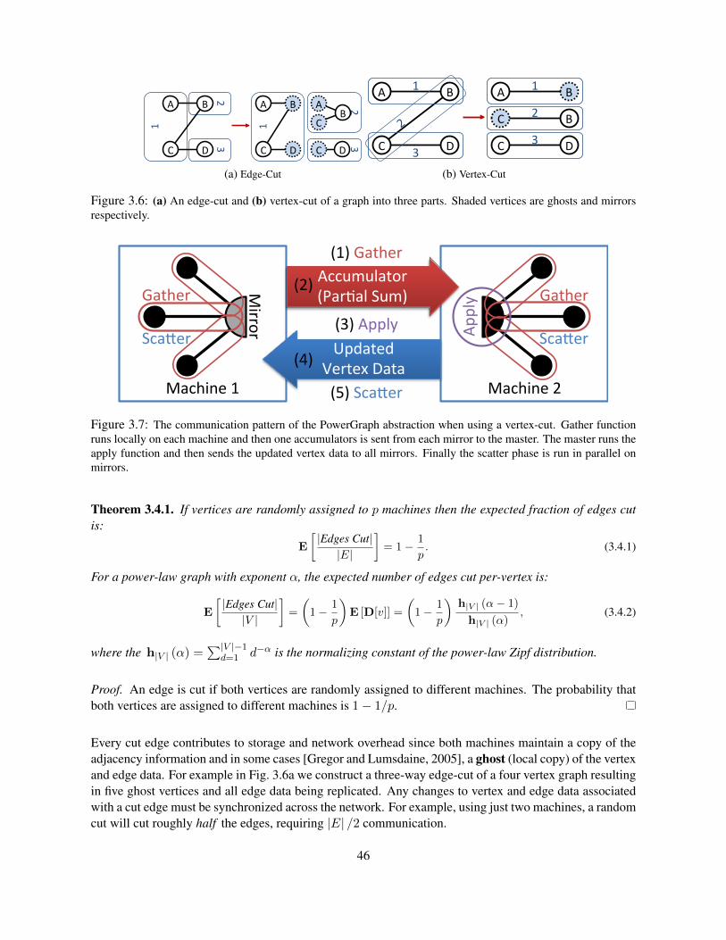
3 2
1 D
A
C
B 2 3
C
D
B A
1
D
A
C C
B
(a) Edge-Cut
B A 1
C D3
C B 2
C D
B A 1
3
(b) Vertex-Cut
Figure 3.6: (a) An edge-cut and (b) vertex-cut of a graph into three parts. Shaded vertices are ghosts and mirrorsrespectively.
Machine(1( Machine(2(
Accumulator((Par4al(Sum)(
Updated((Vertex(Data(
Gather( Mirror(Sca>er(
Gather(
Apply(
Sca>er(
(1)(Gather(
(3)(Apply(
(5)(Sca>er(
(2)(
(4)(
Figure 3.7: The communication pattern of the PowerGraph abstraction when using a vertex-cut. Gather functionruns locally on each machine and then one accumulators is sent from each mirror to the master. The master runs theapply function and then sends the updated vertex data to all mirrors. Finally the scatter phase is run in parallel onmirrors.
Theorem 3.4.1. If vertices are randomly assigned to p machines then the expected fraction of edges cutis:
E
[|Edges Cut||E|
]= 1− 1
p. (3.4.1)
For a power-law graph with exponent α, the expected number of edges cut per-vertex is:
E
[|Edges Cut||V |
]=
(1− 1
p
)E [D[v]] =
(1− 1
p
)h|V | (α− 1)
h|V | (α), (3.4.2)
where the h|V | (α) =∑|V |−1
d=1 d−α is the normalizing constant of the power-law Zipf distribution.
Proof. An edge is cut if both vertices are randomly assigned to different machines. The probability thatboth vertices are assigned to different machines is 1− 1/p.
Every cut edge contributes to storage and network overhead since both machines maintain a copy of theadjacency information and in some cases [Gregor and Lumsdaine, 2005], a ghost (local copy) of the vertexand edge data. For example in Fig. 3.6a we construct a three-way edge-cut of a four vertex graph resultingin five ghost vertices and all edge data being replicated. Any changes to vertex and edge data associatedwith a cut edge must be synchronized across the network. For example, using just two machines, a randomcut will cut roughly half the edges, requiring |E| /2 communication.
46
3.4.1 Balanced p-way Vertex-Cut
By factoring the vertex program along the edges in the graph, The PowerGraph abstraction allows a singlevertex-program to span multiple machines. In Fig. 3.7 a single high degree vertex program has beensplit across two machines with the gather and scatter functions running in parallel on each machine andaccumulator and vertex data being exchanged across the network.
Because the PowerGraph abstraction allows a single vertex-program to span multiple machines, we canimprove work balance and reduce communication and storage overhead by evenly assigning edges tomachines and allowing vertices to span machines. Each machine only stores the edge information for theedges assigned to that machine, evenly distributing the massive amounts of edge data. Since each edge isstored exactly once, changes to edge data do not need to be communicated. However, changes to vertexmust be copied to all the machines it spans, thus the storage and network overhead depend on the numberof machines spanned by each vertex.
We minimize storage and network overhead by limiting the number of machines spanned by each vertex.A balanced p-way vertex-cut formalizes this objective by assigning each edge e ∈ E to a machineA(e) ∈ {1, . . . , p}. Each vertex then spans the set of machines A(v) ⊆ {1, . . . , p} that contain itsadjacent edges. We define the balanced vertex-cut objective:
minA
1
|V |∑v∈V|A(v)| (3.4.3)
s.t. maxm|{e ∈ E |A(e) = m}| , < λ
|E|p
(3.4.4)
where the imbalance factor λ ≥ 1 is a small constant. We use the term replicas of a vertex v to denotethe |A(v)| copies of the vertex v: each machine in A(v) has a replica of v. Because changes to vertexdata are communicated to all replicas, the communication overhead is also given by |A(v)|. The objective(Eq. (3.4.3)) therefore minimizes the average number of replicas in the graph and as a consequence thetotal storage and communication requirements of the PowerGraph engine.
For each vertex v with multiple replicas, one of the replicas is randomly nominated as the master whichmaintains the master version of the vertex data. All remaining replicas of v are then mirrors and maintaina local cached read only copy of the vertex data. (e.g., Fig. 3.6b). For instance, in Fig. 3.6b we constructa three-way vertex-cut of a graph yielding only 2 mirrors. Any changes to the vertex data (e.g., the Applyfunction) must be made to the master which is then immediately replicated to all mirrors.
Vertex-cuts address the major issues associated with edge-cuts in power-law graphs. Percolation theory[Albert et al., 2000] suggests that power-law graphs have good vertex-cuts. Intuitively, by cutting a smallfraction of the very high degree vertices we can quickly shatter a graph. Furthermore, because the balanceconstraint (Eq. (3.4.4)) ensures that edges are uniformly distributed over machines, we naturally achieveimproved work balance even in the presence of very high-degree vertices.
The vertex-cut approach to distributed graph placement is related to work by Catalyurek and Aykanat[1996], Devine et al. [2006] in hypergraph partitioning. In particular, a vertex-cut problem can be cast asa hypergraph-cut problem by converting each edge to a vertex, and each vertex to a hyper-edge. However,since existing hypergraph partitioning can be too time intensive to use effectively on extremely largegraphs, we instead consider the streaming setting where each edge of the graph is accessed exactly once.The streaming graph partitioning setting has been explored in Stanton and Kliot [2011] for the streamingedge-cut problem but did not consider the vertex-cut problem.
47
The simplest method to construct a vertex cut is to randomly assign edges to machines. Random (hashed)edge placement is fully data-parallel, achieves nearly perfect balance on large graphs, and can be appliedin the streaming setting. In the following theorem, we relate the expected normalized replication factor(Eq. (3.4.3)) to the number of machines and the power-law constant α.Theorem 3.4.2 (Randomized Vertex Cuts). A random vertex-cut on p machines has an expected replica-tion:
E
[1
|V |∑v∈V|A(v)|
]=
p
|V |∑v∈V
(1−
(1− 1
p
)D[v]). (3.4.5)
where D[v] denotes the degree of vertex v. For a power-law graph the expected replication (Fig. 3.8a) isdetermined entirely by the power-law constant α:
E
[1
|V |∑v∈V|A(v)|
]= p− p
h|V | (α)
|V |−1∑d=1
(p− 1
p
)dd−α, (3.4.6)
where h|V | (α) =∑|V |−1
d=1 d−α is the normalizing constant of the power-law Zipf distribution.
Proof. By linearity of expectation:
E
[1
|V |∑v∈V|A(v)|
]=
1
|V |∑v∈V
E [|A(v)|] , (3.4.7)
The expected replication E [|A(v)|] of a single vertex v can be computed by considering the process ofrandomly assigning the D[v] edges adjacent to v. Let the indicator Xi denote the event that vertex v hasat least one of its edges on machine i. The expectation E [Xi] is then:
E [Xi] = 1−P (v has no edges on machine i) (3.4.8)
= 1−(
1− 1
p
)D[v]
, (3.4.9)
The expected replication factor for vertex v is then:
E [|A(v)|] =
p∑i=1
E [Xi] = p
(1−
(1− 1
p
)D[v]). (3.4.10)
Treating D[v] as a Zipf random variable:
E
[1
|V |∑v∈V|A(v)|
]=
p
|V |∑v∈V
(1−E
[(p− 1
p
)D[v]])
, (3.4.11)
and taking the expectation under P (d) = d−α/h|V | (α):
E
[(1− 1
p
)D[v]]
=1
h|V | (α)
|V |−1∑d=1
(1− 1
p
)dd−α. (3.4.12)
48
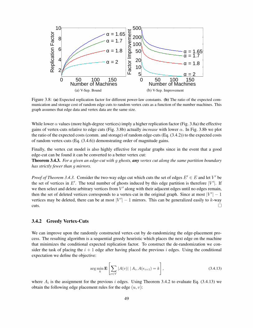
0 50 100 150
2
4
6
8
10α = 1.65α = 1.7
α = 1.8
α = 2
Number of Machines
Rep
licat
ion
Fac
tor
(a) V-Sep. Bound
0 50 100 1505
1020
50100200
500
α = 1.65α = 1.7
α = 1.8
α = 2
Number of Machines
Fac
tor
Impr
ovem
ent
(b) V-Sep. Improvement
Figure 3.8: (a) Expected replication factor for different power-law constants. (b) The ratio of the expected com-munication and storage cost of random edge cuts to random vertex cuts as a function of the number machines. Thisgraph assumes that edge data and vertex data are the same size.
While lower α values (more high-degree vertices) imply a higher replication factor (Fig. 3.8a) the effectivegains of vertex-cuts relative to edge cuts (Fig. 3.8b) actually increase with lower α. In Fig. 3.8b we plotthe ratio of the expected costs (comm. and storage) of random edge-cuts (Eq. (3.4.2)) to the expected costsof random vertex-cuts (Eq. (3.4.6)) demonstrating order of magnitude gains.
Finally, the vertex cut model is also highly effective for regular graphs since in the event that a goodedge-cut can be found it can be converted to a better vertex cut:Theorem 3.4.3. For a given an edge-cut with g ghosts, any vertex cut along the same partition boundaryhas strictly fewer than g mirrors.
Proof of Theorem 3.4.3. Consider the two-way edge cut which cuts the set of edges E′ ∈ E and let V ′ bethe set of vertices in E′. The total number of ghosts induced by this edge partition is therefore |V ′|. Ifwe then select and delete arbitrary vertices from V ′ along with their adjacent edges until no edges remain,then the set of deleted vertices corresponds to a vertex-cut in the original graph. Since at most |V ′| − 1vertices may be deleted, there can be at most |V ′| − 1 mirrors. This can be generalized easily to k-waycuts.
3.4.2 Greedy Vertex-Cuts
We can improve upon the randomly constructed vertex-cut by de-randomizing the edge-placement pro-cess. The resulting algorithm is a sequential greedy heuristic which places the next edge on the machinethat minimizes the conditional expected replication factor. To construct the de-randomization we con-sider the task of placing the i + 1 edge after having placed the previous i edges. Using the conditionalexpectation we define the objective:
arg mink
E
[∑v∈V|A(v)| |Ai, A(ei+1) = k
], (3.4.13)
where Ai is the assignment for the previous i edges. Using Theorem 3.4.2 to evaluate Eq. (3.4.13) weobtain the following edge placement rules for the edge (u, v):
49
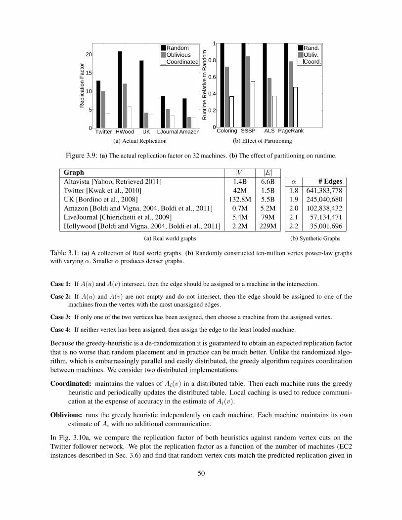
Twitter HWood UK LJournal Amazon0
5
10
15
20
Rep
licat
ion
Fac
tor
RandomObliviousCoordinated
(a) Actual Replication
Coloring SSSP ALS PageRank0
0.2
0.4
0.6
0.8
1
Run
time
Rel
ativ
e to
Ran
dom
Rand.Obliv.Coord.
(b) Effect of Partitioning
Figure 3.9: (a) The actual replication factor on 32 machines. (b) The effect of partitioning on runtime.
Graph |V | |E|Altavista [Yahoo, Retrieved 2011] 1.4B 6.6BTwitter [Kwak et al., 2010] 42M 1.5BUK [Bordino et al., 2008] 132.8M 5.5BAmazon [Boldi and Vigna, 2004, Boldi et al., 2011] 0.7M 5.2MLiveJournal [Chierichetti et al., 2009] 5.4M 79MHollywood [Boldi and Vigna, 2004, Boldi et al., 2011] 2.2M 229M
(a) Real world graphs
α # Edges1.8 641,383,7781.9 245,040,6802.0 102,838,4322.1 57,134,4712.2 35,001,696
(b) Synthetic Graphs
Table 3.1: (a) A collection of Real world graphs. (b) Randomly constructed ten-million vertex power-law graphswith varying α. Smaller α produces denser graphs.
Case 1: If A(u) and A(v) intersect, then the edge should be assigned to a machine in the intersection.
Case 2: If A(u) and A(v) are not empty and do not intersect, then the edge should be assigned to one of themachines from the vertex with the most unassigned edges.
Case 3: If only one of the two vertices has been assigned, then choose a machine from the assigned vertex.
Case 4: If neither vertex has been assigned, then assign the edge to the least loaded machine.
Because the greedy-heuristic is a de-randomization it is guaranteed to obtain an expected replication factorthat is no worse than random placement and in practice can be much better. Unlike the randomized algo-rithm, which is embarrassingly parallel and easily distributed, the greedy algorithm requires coordinationbetween machines. We consider two distributed implementations:
Coordinated: maintains the values of Ai(v) in a distributed table. Then each machine runs the greedyheuristic and periodically updates the distributed table. Local caching is used to reduce communi-cation at the expense of accuracy in the estimate of Ai(v).
Oblivious: runs the greedy heuristic independently on each machine. Each machine maintains its ownestimate of Ai with no additional communication.
In Fig. 3.10a, we compare the replication factor of both heuristics against random vertex cuts on theTwitter follower network. We plot the replication factor as a function of the number of machines (EC2instances described in Sec. 3.6) and find that random vertex cuts match the predicted replication given in
50
8 16 32 48 6412
6
10
14
18
#Machines
Rep
licat
ion
Fac
tor Predicted
Oblivious
Coordinated
Random
(a) Replication Factor (Twitter)
8 16 32 48 640
200
400
600
800
1000
#Machines
Run
time
(sec
s)
Coordinated
Oblivious
Random
(b) Ingress time (Twitter)
Figure 3.10: (a,b) Replication factor and runtime of graph ingress for the Twitter follower network as a functionof the number of machines for random, oblivious, and coordinated vertex-cuts.
Theorem 3.4.2. Furthermore, the greedy heuristics substantially improve upon random placement with anorder of magnitude reduction in the replication factor, and therefore communication and storage costs. Fora fixed number of machines (p = 32), we evaluated (Fig. 3.9a) the replication factor of the two heuristicson five real-world graphs (Table 3.1a). In all cases the greedy heuristics out-perform random placement,while doubling the load time (Fig. 3.10b). The Oblivious heuristic achieves compromise by obtaining arelatively low replication factor while only slightly increasing runtime.
3.5 Abstraction Comparison
In this section, we experimentally characterize the dependence on α and the relationship between fan-in and fan-out by using the Pregel, GraphLab 1, and PowerGraph abstractions to run PageRank on fivesynthetically constructed power-law graphs. Each graph has ten-million vertices and an α ranging from1.8 to 2.2. The graphs were constructed by randomly sampling the out-degree of each vertex from a Zipfdistribution and then adding out-edges such that the in-degree of each vertex is nearly identical. We theninverted each graph to obtain the corresponding power-law fan-in graph. The density of each power-lawgraph is determined by α and therefore each graph has a different number of edges (see Table 3.1b).
We used the GraphLab 1 C++ implementation from Chap. 2 and added instrumentation to track networkusage. As of the writing of the PowerGraph paper [Gonzalez et al., 2012], public implementations ofPregel (e.g., Giraph) were unable to handle even our smaller synthetic problems due to memory limita-tions. Consequently, we used Piccolo [Power and Li, 2010] as a proxy implementation of Pregel sincePiccolo naturally expresses the Pregel abstraction and provides an efficient C++ implementation with dy-namic load-balancing. Finally, we used our implementation of PowerGraph described in Sec. 3.6.
All experiments in this section are evaluated on an eight node Linux cluster. Each node consists of twoquad-core Intel Xeon E5620 processors with 32 GB of RAM and is connected via 1-GigE Ethernet. Allsystems were compiled with GCC 4.4. GraphLab 1 and Piccolo used random edge-cuts while PowerGraphused random vertex-cuts.. Results are averaged over 20 iterations.
51
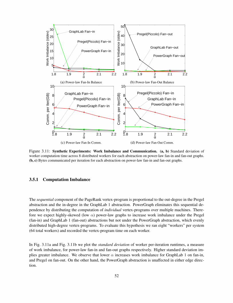
1.8 1.9 2 2.1 2.2
5
10
15
20
25
30
α
Wor
k Im
bala
nce
(std
ev) GraphLab Fan−in
PowerGraph Fan−in
Pregel(Piccolo) Fan−in
(a) Power-law Fan-In Balance
1.8 1.9 2 2.1 2.2
10
20
30
40
50
α
Wor
k Im
bala
nce
(std
ev)
Pregel(Piccolo) Fan−out
GraphLab Fan−out
PowerGraph Fan−out
(b) Power-law Fan-Out Balance
1.8 1.9 2 2.1 2.20
2
4
6
8
10
α
Com
m. p
er It
er(G
B) GraphLab Fan−in
Pregel(Piccolo) Fan−in
PowerGraph Fan−in
(c) Power-law Fan-In Comm.
1.8 1.9 2 2.1 2.20
2
4
6
8
10
α
Com
m. p
er It
er(G
B)
PowerGraph Fan−in
Pregel(Piccolo) Fan−in
GraphLab Fan−in
(d) Power-law Fan-Out Comm.
Figure 3.11: Synthetic Experiments: Work Imbalance and Communication. (a, b) Standard deviation ofworker computation time across 8 distributed workers for each abstraction on power-law fan-in and fan-out graphs.(b, c) Bytes communicated per iteration for each abstraction on power-law fan-in and fan-out graphs.
3.5.1 Computation Imbalance
The sequential component of the PageRank vertex-program is proportional to the out-degree in the Pregelabstraction and the in-degree in the GraphLab 1 abstraction. PowerGraph eliminates this sequential de-pendence by distributing the computation of individual vertex-programs over multiple machines. There-fore we expect highly-skewed (low α) power-law graphs to increase work imbalance under the Pregel(fan-in) and GraphLab 1 (fan-out) abstractions but not under the PowerGraph abstraction, which evenlydistributed high-degree vertex-programs. To evaluate this hypothesis we ran eight “workers” per system(64 total workers) and recorded the vertex-program time on each worker.
In Fig. 3.11a and Fig. 3.11b we plot the standard deviation of worker per-iteration runtimes, a measureof work imbalance, for power-law fan-in and fan-out graphs respectively. Higher standard deviation im-plies greater imbalance. We observe that lower α increases work imbalance for GraphLab 1 on fan-in,and Pregel on fan-out. On the other hand, the PowerGraph abstraction is unaffected in either edge direc-tion.
52
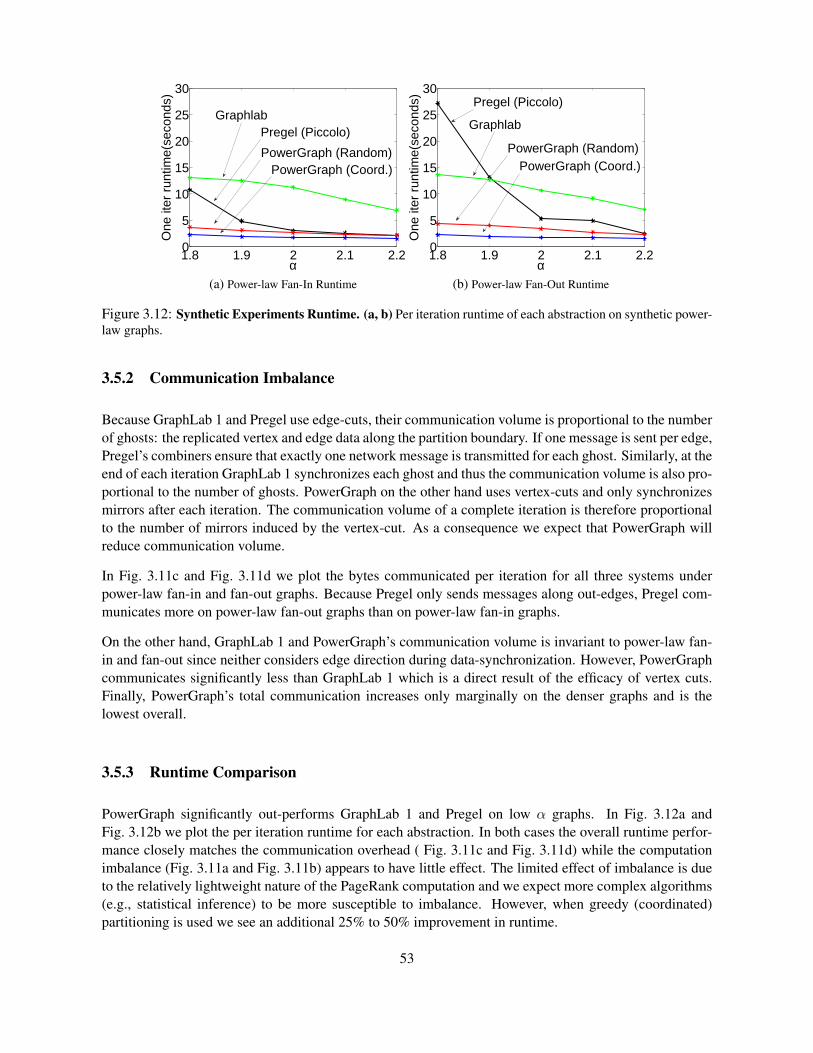
1.8 1.9 2 2.1 2.20
5
10
15
20
25
30
α
One
iter
run
time(
seco
nds)
GraphlabPregel (Piccolo)
PowerGraph (Random)PowerGraph (Coord.)
(a) Power-law Fan-In Runtime
1.8 1.9 2 2.1 2.20
5
10
15
20
25
30
α
One
iter
run
time(
seco
nds) Pregel (Piccolo)
Graphlab
PowerGraph (Random)PowerGraph (Coord.)
(b) Power-law Fan-Out Runtime
Figure 3.12: Synthetic Experiments Runtime. (a, b) Per iteration runtime of each abstraction on synthetic power-law graphs.
3.5.2 Communication Imbalance
Because GraphLab 1 and Pregel use edge-cuts, their communication volume is proportional to the numberof ghosts: the replicated vertex and edge data along the partition boundary. If one message is sent per edge,Pregel’s combiners ensure that exactly one network message is transmitted for each ghost. Similarly, at theend of each iteration GraphLab 1 synchronizes each ghost and thus the communication volume is also pro-portional to the number of ghosts. PowerGraph on the other hand uses vertex-cuts and only synchronizesmirrors after each iteration. The communication volume of a complete iteration is therefore proportionalto the number of mirrors induced by the vertex-cut. As a consequence we expect that PowerGraph willreduce communication volume.
In Fig. 3.11c and Fig. 3.11d we plot the bytes communicated per iteration for all three systems underpower-law fan-in and fan-out graphs. Because Pregel only sends messages along out-edges, Pregel com-municates more on power-law fan-out graphs than on power-law fan-in graphs.
On the other hand, GraphLab 1 and PowerGraph’s communication volume is invariant to power-law fan-in and fan-out since neither considers edge direction during data-synchronization. However, PowerGraphcommunicates significantly less than GraphLab 1 which is a direct result of the efficacy of vertex cuts.Finally, PowerGraph’s total communication increases only marginally on the denser graphs and is thelowest overall.
3.5.3 Runtime Comparison
PowerGraph significantly out-performs GraphLab 1 and Pregel on low α graphs. In Fig. 3.12a andFig. 3.12b we plot the per iteration runtime for each abstraction. In both cases the overall runtime perfor-mance closely matches the communication overhead ( Fig. 3.11c and Fig. 3.11d) while the computationimbalance (Fig. 3.11a and Fig. 3.11b) appears to have little effect. The limited effect of imbalance is dueto the relatively lightweight nature of the PageRank computation and we expect more complex algorithms(e.g., statistical inference) to be more susceptible to imbalance. However, when greedy (coordinated)partitioning is used we see an additional 25% to 50% improvement in runtime.
53
3.6 Implementation and Evaluation
In this section, we describe and evaluate our implementation of the PowerGraph2 abstraction. All ex-periments are performed on a 64 node cluster of Amazon EC2 cc1.4xlarge Linux instances. Eachinstance has two quad core Intel Xeon X5570 processors with 23GB of RAM, and is connected via 10GigE Ethernet. PowerGraph was written in C++ and compiled with GCC 4.5.
We implemented three variations of the PowerGraph abstraction. To demonstrate their relative implemen-tation complexity, we provide the line counts, excluding common support code:
Bulk Synchronous (Sync): A fully synchronous implementation of PowerGraph as described in Sec. 3.3.3.1. [600lines]
Asynchronous (Async): An asynchronous implementation of PowerGraph which allows arbitrary interleaving ofvertex-programs Sec. 3.3.3.2. [900 lines]
Asynchronous Serializable (Async+S): An asynchronous implementation of PowerGraph which guarantees seri-alizability of all vertex-programs (equivalent to “edge consistency” in GraphLab 1). [1600 lines]
In all cases the system is entirely symmetric with no single coordinating instance or scheduler. Eachinstances is given the list of other machines and start by reading a unique subset of the graph data filesfrom HDFS. TCP connections are opened with other machines as needed to build the distributed graphand run the engine.
3.6.1 Graph Loading and Placement
The graph structure and data are loaded from a collection of text files stored in a distributed file-system(HDFS) by all instances in parallel. Each machine loads a separate subset of files (determined by hashing)and applies one of the three distributed graph partitioning algorithms to place the data as it is loaded. Asa consequence partitioning is accomplished in parallel and data is immediately placed in its final location.Unless specified, all experiments were performed using the oblivious algorithm. Once computation iscomplete, the final vertex and edge data are saved back to the distributed file-system in parallel.
In Fig. 3.9b, we evaluate the performance of a collection of algorithms varying the partitioning procedure.Our simple partitioning heuristics are able to improve performance significantly across all algorithms,decreasing runtime and memory utilization. Furthermore, the runtime scales linearly with the replicationfactor: halving the replication factor approximately halves runtime.
3.6.2 Synchronous Engine (Sync)
Our synchronous implementation closely follows the description in Sec. 3.3.3.1. Each machine runs asingle multi-threaded instance to maximally utilize the multi-core architecture. We rely on backgroundcommunication to achieve computation/communication interleaving. The synchronous engine’s fully de-terministic execution makes it easy to reason about programmatically and minimizes effort needed fortuning and performance optimizations.
2PowerGraph is now part of the GraphLab2 open source project and can be obtained from http://graphlab.org.
54
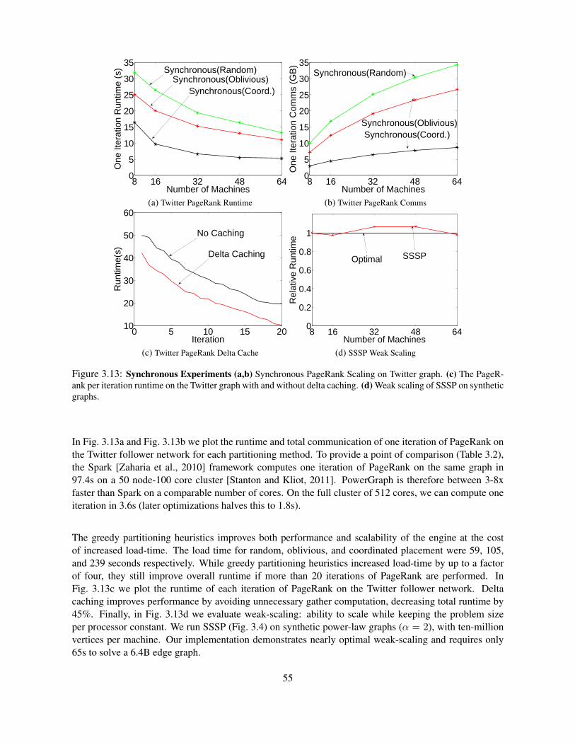
8 16 32 48 640
5
10
15
20
25
30
35
Number of Machines
One
Iter
atio
n R
untim
e (s
) Synchronous(Random)Synchronous(Oblivious)
Synchronous(Coord.)
(a) Twitter PageRank Runtime
8 16 32 48 640
5
10
15
20
25
30
35
Number of Machines
One
Iter
atio
n C
omm
s (G
B)
Synchronous(Oblivious)Synchronous(Coord.)
Synchronous(Random)
(b) Twitter PageRank Comms
0 5 10 15 2010
20
30
40
50
60
Iteration
Run
time(
s)
No Caching
Delta Caching
(c) Twitter PageRank Delta Cache
8 16 32 48 640
0.2
0.4
0.6
0.8
1
Number of Machines
Rel
ativ
e R
untim
e
Optimal SSSP
(d) SSSP Weak Scaling
Figure 3.13: Synchronous Experiments (a,b) Synchronous PageRank Scaling on Twitter graph. (c) The PageR-ank per iteration runtime on the Twitter graph with and without delta caching. (d) Weak scaling of SSSP on syntheticgraphs.
In Fig. 3.13a and Fig. 3.13b we plot the runtime and total communication of one iteration of PageRank onthe Twitter follower network for each partitioning method. To provide a point of comparison (Table 3.2),the Spark [Zaharia et al., 2010] framework computes one iteration of PageRank on the same graph in97.4s on a 50 node-100 core cluster [Stanton and Kliot, 2011]. PowerGraph is therefore between 3-8xfaster than Spark on a comparable number of cores. On the full cluster of 512 cores, we can compute oneiteration in 3.6s (later optimizations halves this to 1.8s).
The greedy partitioning heuristics improves both performance and scalability of the engine at the costof increased load-time. The load time for random, oblivious, and coordinated placement were 59, 105,and 239 seconds respectively. While greedy partitioning heuristics increased load-time by up to a factorof four, they still improve overall runtime if more than 20 iterations of PageRank are performed. InFig. 3.13c we plot the runtime of each iteration of PageRank on the Twitter follower network. Deltacaching improves performance by avoiding unnecessary gather computation, decreasing total runtime by45%. Finally, in Fig. 3.13d we evaluate weak-scaling: ability to scale while keeping the problem sizeper processor constant. We run SSSP (Fig. 3.4) on synthetic power-law graphs (α = 2), with ten-millionvertices per machine. Our implementation demonstrates nearly optimal weak-scaling and requires only65s to solve a 6.4B edge graph.
55
3.6.3 Asynchronous Engine (Async)
We implemented the asynchronous PowerGraph execution model (Sec. 3.3.3.2) using a simple state ma-chine for each vertex which can be either: INACTIVE, GATHER, APPLY or SCATTER. Once activated,a vertex enters the gathering state and is placed in a local scheduler which assigns cores to active verticesallowing many vertex-programs to run simultaneously thereby hiding communication latency. While arbi-trary interleaving of vertex programs is permitted, we avoid data races by ensuring that individual gather,apply, and scatter calls have exclusive access to their arguments.
We evaluate the performance of the Async engine by running PageRank on the Twitter follower network.In Fig. 3.14a, we plot throughput (number of vertex-program operations per second) against the numberof machines. Throughput increases moderately with both the number of machines as well as improvedpartitioning. We evaluate the gains associated with delta caching (Sec. 3.3.2) by measuring throughputas a function of time (Fig. 3.14b) with caching enabled and with caching disabled. Caching allows thealgorithm to converge faster with fewer operations. Surprisingly, when caching is disabled, the through-put increases over time. Further analysis reveals that the computation gradually focuses on high-degreevertices, increasing the computation/communication ratio.
We evaluate the graph coloring vertex-program (Fig. 3.4) which cannot be run synchronously since allvertices would change to the same color on every iteration. Graph coloring is a proxy for many MLalgorithms [Gonzalez et al., 2011]. In Fig. 3.14c we evaluate weak-scaling on synthetic power-law graphs(α = 2) with five-million vertices per machine and find that the Async engine performs nearly optimally.The slight increase in runtime may be attributed to an increase in the number of colors due to increasinggraph size.
3.6.4 Async. Serializable Engine (Async+S)
The Async engine is useful for a broad range of tasks, providing high throughput and performance. How-ever, unlike the synchronous engine, the asynchronous engine is difficult to reason about programmati-cally. We therefore extended the Async engine to enforce serializability.
The Async+S engine ensures serializability by preventing adjacent vertex-programs from running simulta-neously. Ensuring serializability for graph-parallel computation is equivalent to solving the dining philoso-phers problem where each vertex is a philosopher, and each edge is a fork. GraphLab 1 (Sec. 2.3.1 andSec. 2.4.2.2) implements Dijkstra’s solution [Dijkstra, 1971] where forks are acquired sequentially ac-cording to a total ordering. Instead, we implement the Chandy-Misra solution [Chandy and Misra, 1984]which acquires all forks simultaneously, permitting a high degree of parallelism. We extend the Chandy-Misra solution to the vertex-cut setting by enabling each vertex replica to request only forks for localedges and using a simple consensus protocol to establish when all replicas have succeeded. The details ofthe algorithm are described in Appendix A
We evaluate the scalability and computational efficiency of the Async+S engine on the graph coloring task.We observe in Fig. 3.14c that the amount of achieved parallelism does not increase linearly with the num-ber of vertices. Because the density (i.e., contention) of power-law graphs increases super-linearly withthe number of vertices, we do not expect the amount of serializable parallelism to increase linearly.
In Fig. 3.14d, we plot the proportion of edges that satisfy the coloring condition (both vertices havedifferent colors) for both the Async and the Async+S engines. While the Async engine quickly satisfies
56
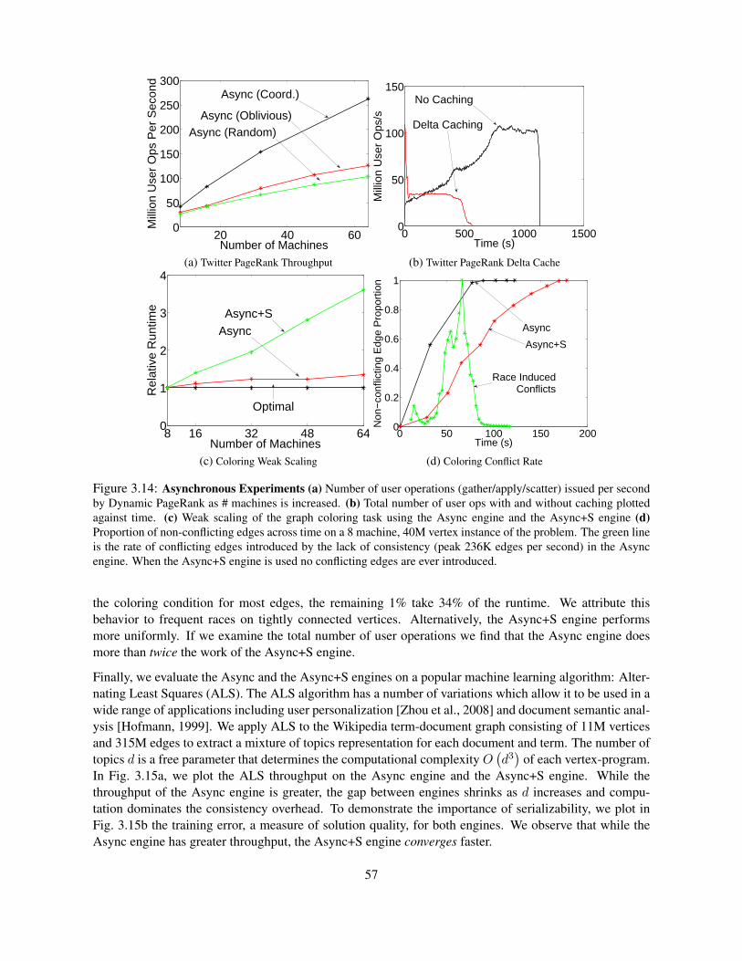
20 40 600
50
100
150
200
250
300
Number of Machines
Mill
ion
Use
r O
ps P
er S
econ
d
Async (Coord.)
Async (Random)Async (Oblivious)
(a) Twitter PageRank Throughput
0 500 1000 15000
50
100
150
Time (s)
Mill
ion
Use
r O
ps/s
No Caching
Delta Caching
(b) Twitter PageRank Delta Cache
8 16 32 48 640
1
2
3
4
Number of Machines
Rel
ativ
e R
untim
e Async+S
Async
Optimal
(c) Coloring Weak Scaling
0 50 100 150 2000
0.2
0.4
0.6
0.8
1
Time (s)
Non
−co
nflic
ting
Edg
e P
ropo
rtio
n
Async
Async+S
Race InducedConflicts
(d) Coloring Conflict Rate
Figure 3.14: Asynchronous Experiments (a) Number of user operations (gather/apply/scatter) issued per secondby Dynamic PageRank as # machines is increased. (b) Total number of user ops with and without caching plottedagainst time. (c) Weak scaling of the graph coloring task using the Async engine and the Async+S engine (d)Proportion of non-conflicting edges across time on a 8 machine, 40M vertex instance of the problem. The green lineis the rate of conflicting edges introduced by the lack of consistency (peak 236K edges per second) in the Asyncengine. When the Async+S engine is used no conflicting edges are ever introduced.
the coloring condition for most edges, the remaining 1% take 34% of the runtime. We attribute thisbehavior to frequent races on tightly connected vertices. Alternatively, the Async+S engine performsmore uniformly. If we examine the total number of user operations we find that the Async engine doesmore than twice the work of the Async+S engine.
Finally, we evaluate the Async and the Async+S engines on a popular machine learning algorithm: Alter-nating Least Squares (ALS). The ALS algorithm has a number of variations which allow it to be used in awide range of applications including user personalization [Zhou et al., 2008] and document semantic anal-ysis [Hofmann, 1999]. We apply ALS to the Wikipedia term-document graph consisting of 11M verticesand 315M edges to extract a mixture of topics representation for each document and term. The number oftopics d is a free parameter that determines the computational complexity O
(d3)
of each vertex-program.In Fig. 3.15a, we plot the ALS throughput on the Async engine and the Async+S engine. While thethroughput of the Async engine is greater, the gap between engines shrinks as d increases and compu-tation dominates the consistency overhead. To demonstrate the importance of serializability, we plot inFig. 3.15b the training error, a measure of solution quality, for both engines. We observe that while theAsync engine has greater throughput, the Async+S engine converges faster.
57
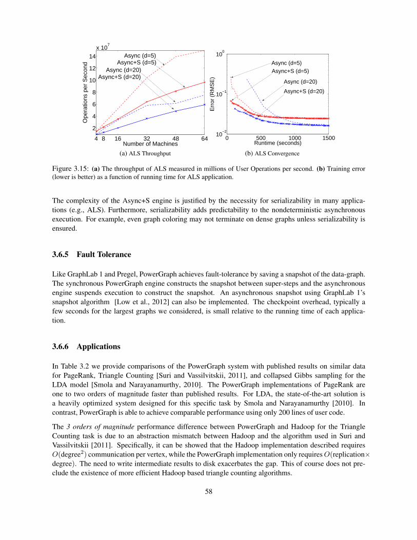
4 8 16 32 48 64
2
4
6
8
10
12
14
x 107
Number of Machines
Ope
ratio
ns p
er S
econ
d Async+S (d=5)Async (d=5)
Async (d=20)Async+S (d=20)
(a) ALS Throughput
0 500 1000 150010
−2
10−1
100
Runtime (seconds)
Err
or (
RM
SE
)
Async (d=5)
Async+S (d=20)
Async (d=20)
Async+S (d=5)
(b) ALS Convergence
Figure 3.15: (a) The throughput of ALS measured in millions of User Operations per second. (b) Training error(lower is better) as a function of running time for ALS application.
The complexity of the Async+S engine is justified by the necessity for serializability in many applica-tions (e.g., ALS). Furthermore, serializability adds predictability to the nondeterministic asynchronousexecution. For example, even graph coloring may not terminate on dense graphs unless serializability isensured.
3.6.5 Fault Tolerance
Like GraphLab 1 and Pregel, PowerGraph achieves fault-tolerance by saving a snapshot of the data-graph.The synchronous PowerGraph engine constructs the snapshot between super-steps and the asynchronousengine suspends execution to construct the snapshot. An asynchronous snapshot using GraphLab 1’ssnapshot algorithm [Low et al., 2012] can also be implemented. The checkpoint overhead, typically afew seconds for the largest graphs we considered, is small relative to the running time of each applica-tion.
3.6.6 Applications
In Table 3.2 we provide comparisons of the PowerGraph system with published results on similar datafor PageRank, Triangle Counting [Suri and Vassilvitskii, 2011], and collapsed Gibbs sampling for theLDA model [Smola and Narayanamurthy, 2010]. The PowerGraph implementations of PageRank areone to two orders of magnitude faster than published results. For LDA, the state-of-the-art solution isa heavily optimized system designed for this specific task by Smola and Narayanamurthy [2010]. Incontrast, PowerGraph is able to achieve comparable performance using only 200 lines of user code.
The 3 orders of magnitude performance difference between PowerGraph and Hadoop for the TriangleCounting task is due to an abstraction mismatch between Hadoop and the algorithm used in Suri andVassilvitskii [2011]. Specifically, it can be showed that the Hadoop implementation described requiresO(degree2) communication per vertex, while the PowerGraph implementation only requiresO(replication×degree). The need to write intermediate results to disk exacerbates the gap. This of course does not pre-clude the existence of more efficient Hadoop based triangle counting algorithms.
58
3.7 Conclusion
The need to reason about large-scale graph-structured data has driven the development of new graph-parallel abstractions such as GraphLab 1 and Pregel. However graphs derived from real-world phenom-ena often exhibit power-law degree distributions, which are difficult to partition and can lead to workimbalance and substantially increased communication and storage.
To address these challenges, we introduced the PowerGraph abstraction which exploits the Gather-Apply-Scatter model of computation to factor vertex-programs over edges, splitting high-degree vertices andexposing greater parallelism in natural graphs. We then introduced vertex-cuts and a collection of fastgreedy heuristics to substantially reduce the storage and communication costs of large distributed power-law graphs. We theoretically related the power-law constant to the communication and storage require-ments of the PowerGraph system and empirically evaluate our analysis by comparing against GraphLab 1and Pregel. Finally, we evaluate the PowerGraph system on several large-scale problems using a 64 nodeEC2 cluster and demonstrating the scalability and efficiency and in many cases order of magnitude gainsover published results.
The PowerGraph abstraction is highly expressive, capable of representing a large number of graph algo-rithms, matrix factorization algorithms, graphical model inference methods, etc. The GraphLab 2.1 releaseat http://graphlab.org includes our distributed implementation of over 24 different algorithmsspread over 7 toolkits of Clustering, Computer Vision, Collaborative Filtering, Graph Analytics, Graphi-cal Models, Linear Solvers and Topic Modeling, and has been downloaded thousands of times.
Finally, Kyrola et al. [2012] presents GraphChi: an efficient single-machine disk-based implementation ofthe GraphLab 1 abstraction. Impressively, it is able to significantly out-perform large Hadoop deploymentson many graph problems while using only a single machine: performing one iteration of PageRank on theTwitter Graph in only 158s (PowerGraph: 1.8s). The techniques described in GraphChi can be used toadd out-of-core storage to PowerGraph.
Out key contributions are:
• An analysis of the challenges of power-law graphs in distributed graph computation and the limita-tions of existing graph parallel abstractions (Sec. 3.1.2.1).
• The PowerGraph abstraction (Sec. 3.3) which factors individual vertex-programs.
• A delta caching procedure which allows computation state to be dynamically maintained (Sec. 3.3.2).
• A new fast approach to data layout for power-law graphs in distributed environments (Sec. 3.4).
• An theoretical characterization of network and storage (Theorem 3.4.2, Theorem 3.4.3).
• A high-performance open-source implementation of the PowerGraph abstraction (Sec. 3.6).
• A comprehensive evaluation of three implementations of PowerGraph on a large EC2 deploymentusing real-world ML applications (Sec. 3.5 and 3.6).
/ /
59
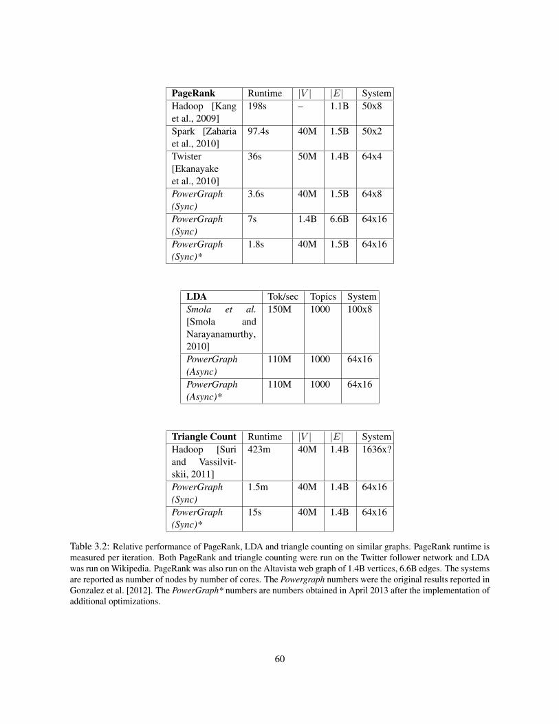
PageRank Runtime |V | |E| SystemHadoop [Kanget al., 2009]
198s – 1.1B 50x8
Spark [Zahariaet al., 2010]
97.4s 40M 1.5B 50x2
Twister[Ekanayakeet al., 2010]
36s 50M 1.4B 64x4
PowerGraph(Sync)
3.6s 40M 1.5B 64x8
PowerGraph(Sync)
7s 1.4B 6.6B 64x16
PowerGraph(Sync)*
1.8s 40M 1.5B 64x16
LDA Tok/sec Topics SystemSmola et al.[Smola andNarayanamurthy,2010]
150M 1000 100x8
PowerGraph(Async)
110M 1000 64x16
PowerGraph(Async)*
110M 1000 64x16
Triangle Count Runtime |V | |E| SystemHadoop [Suriand Vassilvit-skii, 2011]
423m 40M 1.4B 1636x?
PowerGraph(Sync)
1.5m 40M 1.4B 64x16
PowerGraph(Sync)*
15s 40M 1.4B 64x16
Table 3.2: Relative performance of PageRank, LDA and triangle counting on similar graphs. PageRank runtime ismeasured per iteration. Both PageRank and triangle counting were run on the Twitter follower network and LDAwas run on Wikipedia. PageRank was also run on the Altavista web graph of 1.4B vertices, 6.6B edges. The systemsare reported as number of nodes by number of cores. The Powergraph numbers were the original results reported inGonzalez et al. [2012]. The PowerGraph* numbers are numbers obtained in April 2013 after the implementation ofadditional optimizations.
60
Chapter 4
WarpGraph
Fine Grained Data-Parallelism for Usability
In the previous chapter, we presented the PowerGraph abstraction which restricts the abstraction to thestrict Gather-Apply-Scatter model. And in doing so, exposed many optimization opportunities, providinglarge performance gains, and raising the bar for some common benchmarks. In this chapter, we addressthe usability and expressiveness issues of PowerGraph through the use of fine grained abstractions.
In Sec. 4.1 we begin by describing the limitations of the PowerGraph abstraction and show how Power-Graph is difficult to use in practice. To resolve the usability issues with PowerGraph, we introduce theWarpGraph abstraction in Sec. 4.2 which relaxes the restrictions in PowerGraph through the use of fine-grained data-parallel primitives. Through several examples, we show that the WarpGraph abstraction iseasier to use and results in more readable code.
Finally, in Sec. 4.3 we describe an efficient distributed, asynchronous implementation of the WarpGraphabstraction which makes use of user-mode context switching and coroutines to hide communication la-tency. We evaluate the implementation on three challenging tasks and show that WarpGraph significantlyout-performs the PowerGraph asynchronous engine, and can achieve nearly half the throughput rate of thePowerGraph synchronous engine. The performance of the WarpGraph implementation demonstrates thatefficient distributed asynchronous computation is feasible even on commodity hardware.
4.1 PowerGraph Limitations
While the PowerGraph abstraction appears to be highly expressive, it has two key limitations. Firstly,the PowerGraph abstraction is insufficiently expressive for complex vertex programs. And secondly, thePowerGraph abstraction is difficult to work with in practice. We further elaborate on these two limita-tions.
61
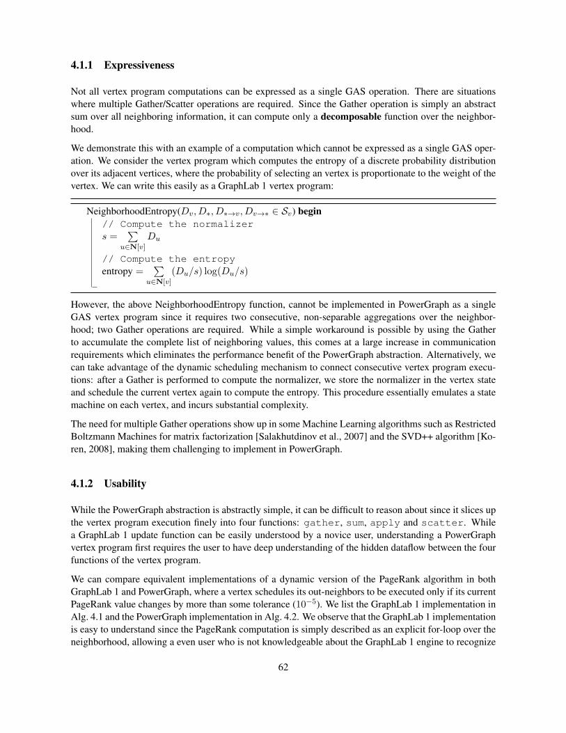
4.1.1 Expressiveness
Not all vertex program computations can be expressed as a single GAS operation. There are situationswhere multiple Gather/Scatter operations are required. Since the Gather operation is simply an abstractsum over all neighboring information, it can compute only a decomposable function over the neighbor-hood.
We demonstrate this with an example of a computation which cannot be expressed as a single GAS oper-ation. We consider the vertex program which computes the entropy of a discrete probability distributionover its adjacent vertices, where the probability of selecting an vertex is proportionate to the weight of thevertex. We can write this easily as a GraphLab 1 vertex program:
NeighborhoodEntropy(Dv, D∗, D∗→v, Dv→∗ ∈ Sv) begin// Compute the normalizers =
∑u∈N[v]
Du
// Compute the entropyentropy =
∑u∈N[v]
(Du/s) log(Du/s)
However, the above NeighborhoodEntropy function, cannot be implemented in PowerGraph as a singleGAS vertex program since it requires two consecutive, non-separable aggregations over the neighbor-hood; two Gather operations are required. While a simple workaround is possible by using the Gatherto accumulate the complete list of neighboring values, this comes at a large increase in communicationrequirements which eliminates the performance benefit of the PowerGraph abstraction. Alternatively, wecan take advantage of the dynamic scheduling mechanism to connect consecutive vertex program execu-tions: after a Gather is performed to compute the normalizer, we store the normalizer in the vertex stateand schedule the current vertex again to compute the entropy. This procedure essentially emulates a statemachine on each vertex, and incurs substantial complexity.
The need for multiple Gather operations show up in some Machine Learning algorithms such as RestrictedBoltzmann Machines for matrix factorization [Salakhutdinov et al., 2007] and the SVD++ algorithm [Ko-ren, 2008], making them challenging to implement in PowerGraph.
4.1.2 Usability
While the PowerGraph abstraction is abstractly simple, it can be difficult to reason about since it slices upthe vertex program execution finely into four functions: gather, sum, apply and scatter. Whilea GraphLab 1 update function can be easily understood by a novice user, understanding a PowerGraphvertex program first requires the user to have deep understanding of the hidden dataflow between the fourfunctions of the vertex program.
We can compare equivalent implementations of a dynamic version of the PageRank algorithm in bothGraphLab 1 and PowerGraph, where a vertex schedules its out-neighbors to be executed only if its currentPageRank value changes by more than some tolerance (10−5). We list the GraphLab 1 implementation inAlg. 4.1 and the PowerGraph implementation in Alg. 4.2. We observe that the GraphLab 1 implementationis easy to understand since the PageRank computation is simply described as an explicit for-loop over theneighborhood, allowing a even user who is not knowledgeable about the GraphLab 1 engine to recognize
62
PageRankUpdate(Dv, D∗, D∗→v, Dv→∗ ∈ Sv) {prev_pagerank = Dv.rank
// compute the sum, iterate over all in neighbors
new_pagerank = 0.15ForEach(u ∈ InNeighbors(v)) {new_pagerank = new_pagerank + 0.85 ×Du.rank / OutDegree(u)
}Dv.rank = new_pagerank
// Reschedule if PageRank changes sufficiently
if(|new_pagerank - prev_pagerank| > ε) {ForEach(u ∈ OutNeighbors(v)) {Schedule(u)
}}
}
Figure 4.1: Dynamic PageRank Graphlab 1 Update Function.
the computation. On the other hand, the PowerGraph implementation in Alg. 4.2 can be difficult to followsince the gather function is implicitly executed over the neighborhood, and the sum function describesan implicit aggregation operation. As a result, a user must have good familiarity with the PowerGraphengine to understand the behavior of the vertex program.
63
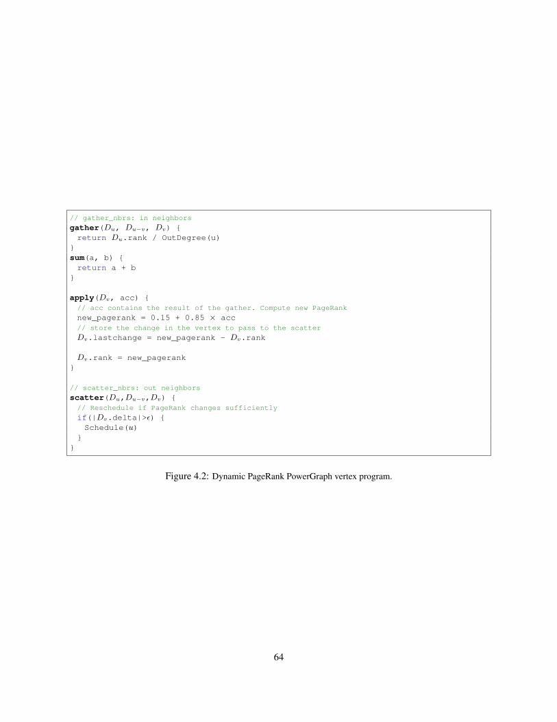
// gather_nbrs: in neighbors
gather(Du, Du−v, Dv) {return Du.rank / OutDegree(u)
}sum(a, b) {return a + b
}
apply(Dv, acc) {// acc contains the result of the gather. Compute new PageRank
new_pagerank = 0.15 + 0.85 × acc// store the change in the vertex to pass to the scatter
Dv.lastchange = new_pagerank - Dv.rank
Dv.rank = new_pagerank}
// scatter_nbrs: out neighbors
scatter(Du,Du−v,Dv) {// Reschedule if PageRank changes sufficiently
if(|Dv.delta|>ε) {Schedule(u)
}}
Figure 4.2: Dynamic PageRank PowerGraph vertex program.
64
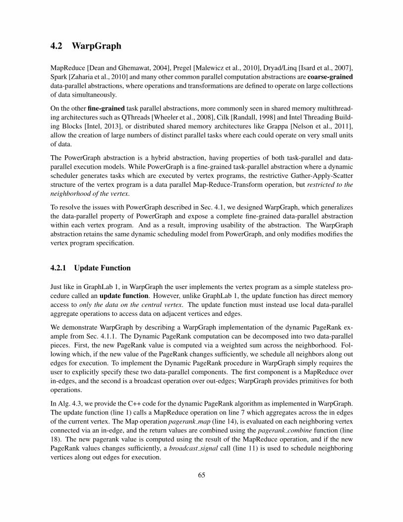
4.2 WarpGraph
MapReduce [Dean and Ghemawat, 2004], Pregel [Malewicz et al., 2010], Dryad/Linq [Isard et al., 2007],Spark [Zaharia et al., 2010] and many other common parallel computation abstractions are coarse-graineddata-parallel abstractions, where operations and transformations are defined to operate on large collectionsof data simultaneously.
On the other fine-grained task parallel abstractions, more commonly seen in shared memory multithread-ing architectures such as QThreads [Wheeler et al., 2008], Cilk [Randall, 1998] and Intel Threading Build-ing Blocks [Intel, 2013], or distributed shared memory architectures like Grappa [Nelson et al., 2011],allow the creation of large numbers of distinct parallel tasks where each could operate on very small unitsof data.
The PowerGraph abstraction is a hybrid abstraction, having properties of both task-parallel and data-parallel execution models. While PowerGraph is a fine-grained task-parallel abstraction where a dynamicscheduler generates tasks which are executed by vertex programs, the restrictive Gather-Apply-Scatterstructure of the vertex program is a data parallel Map-Reduce-Transform operation, but restricted to theneighborhood of the vertex.
To resolve the issues with PowerGraph described in Sec. 4.1, we designed WarpGraph, which generalizesthe data-parallel property of PowerGraph and expose a complete fine-grained data-parallel abstractionwithin each vertex program. And as a result, improving usability of the abstraction. The WarpGraphabstraction retains the same dynamic scheduling model from PowerGraph, and only modifies modifies thevertex program specification.
4.2.1 Update Function
Just like in GraphLab 1, in WarpGraph the user implements the vertex program as a simple stateless pro-cedure called an update function. However, unlike GraphLab 1, the update function has direct memoryaccess to only the data on the central vertex. The update function must instead use local data-parallelaggregate operations to access data on adjacent vertices and edges.
We demonstrate WarpGraph by describing a WarpGraph implementation of the dynamic PageRank ex-ample from Sec. 4.1.1. The Dynamic PageRank computation can be decomposed into two data-parallelpieces. First, the new PageRank value is computed via a weighted sum across the neighborhood. Fol-lowing which, if the new value of the PageRank changes sufficiently, we schedule all neighbors along outedges for execution. To implement the Dynamic PageRank procedure in WarpGraph simply requires theuser to explicitly specify these two data-parallel components. The first component is a MapReduce overin-edges, and the second is a broadcast operation over out-edges; WarpGraph provides primitives for bothoperations.
In Alg. 4.3, we provide the C++ code for the dynamic PageRank algorithm as implemented in WarpGraph.The update function (line 1) calls a MapReduce operation on line 7 which aggregates across the in edgesof the current vertex. The Map operation pagerank map (line 14), is evaluated on each neighboring vertexconnected via an in-edge, and the return values are combined using the pagerank combine function (line18). The new pagerank value is computed using the result of the MapReduce operation, and if the newPageRank values changes sufficiently, a broadcast signal call (line 11) is used to schedule neighboringvertices along out edges for execution.
65
PageRankUpdate(Dv) {prev_pagerank = Dv.rank// compute a map reduce over the neighborhood selecting only the in edges
new_pagerank = 0.15 + 0.85 *map_reduce_neighbors(pagerank_map, pagerank_combine, IN_EDGES)
Dv.rank = new_pagerank
if (|new_pagerank - prev_pagerank| > ε) {broadcast(OUT_EDGES)
}}
// helper functions
pagerank_map(Du,Du−v,Dv) {return Du.rank / OutDegree(u)
}
pagerank_combine(a, b) {return a + b
}
Figure 4.3: Dynamic PageRank WarpGraph Update Function.
Comparing the WarpGraph PageRank implementation against the GraphLab 1 (Alg. 4.1) and PowerGraph(Alg. 4.2) versions, we observe that the WarpGraph implementation is as short as the GraphLab 1 updatefunction, and just as easy to understand. Further note that while we implemented pagerank map andpagerank combine as separate functions, under certain languages with functional capabilities, these canbe implemented as inline lambdas, further simplifying the code.
The WarpGraph implementation is able to both maintain the simplicity of the GraphLab 1 update func-tion, and like PowerGraph, is able to explicitly expose the available parallelism available in the neighbor-hood aggregate operations. WarpGraph therefore combines the benefits of both GraphLab 1 and Power-Graph.
4.2.2 Fine Grained Data-Parallel Primitives
The PageRank example demonstrated two primitives: MapReduce which computes an aggregate overthe neighborhood, and Broadcast which schedules a set of neighbors for execution. In this section, weformally define these two primitives as well a few other useful primitives which add richness to the ab-straction and expand the space of algorithms we can describe efficiently.
Where the update function is executed on vertex u, the following local primitives are available:
MapReduce Equivalent to the Gather operation. Performs an aggregation over the neighborhood.
Transform Equivalent to the Scatter operation. Modifies adjacent edges.
Broadcast Schedules a subset of neighbors depending on a user-defined selector operation.
DHTGather and DHTScatter Reads and writes values from a Distributed Hash Table (DHT).
66
We now describe the exact behavior of these primitives in detail. We use the notation Du to identify thedata on vertex u, and use the notation Du−v to identify the data on the edge edge (u, v).
4.2.2.1 MapReduce
The MapReduce primitive as demonstrated in the PageRank example in Sec. 4.2.1 allows the update func-tion to compute an aggregate over the neighborhood of the vertex, and provides the same functionality asthe Gather operation in PowerGraph. The MapReduce operation takes three arguments: a map function,a combiner, and the set of edges to aggregate over.
result = MapReduce(MapFunction, CombineFunction, EdgeSet)
MapFunction : (Du, Du−v, Dv)→ T
CombineFunction : (T left, T right)→ T
EdgeSet ∈ {IN EDGES,OUT EDGES,ALL EDGES}
The MapReduce operation is semantically equivalent to:
MapReduce(MapFunction, CombineFunction, EdgeSet) beginfirst = Trueacc← Emptyforeach neighbor u in EdgeSet do
mapresult←MapFunction(Du, Du−v, Dv)if first then
first = Falseacc← mapresult
elseacc← CombineFunction(acc, mapresult)
return acc
An overload is provided for the simpler case where MapFunction only needs the value of of the neighbor-ing vertex. In which case, the MapFunction has the simpler form:
MapFunction : (Dv)→ T
4.2.2.2 Transform
The Transform primitive provides the same functionality as the Scatter operation in PowerGraph, and al-lows the update function to make modifications to the edges adjacent to the current vertex. The Transformoperation takes two arguments: a transform function, and the set of edges to transform.
Transform(TransformFunction, EdgeSet)
TransformFunction : (Du, Du−v, Dv)→ Du−v
EdgeSet ∈ {IN EDGES,OUT EDGES,ALL EDGES}
67
The transform operation is semantically equivalent to:
Transform(TransformFunction, EdgeSet) beginforeach neighbor u in EdgeSet do
Du−v ← TransformFunction(Du, Du−v, Dv)
4.2.2.3 Broadcast
The Broadcast primitive allows the update function to selectively choose a subset of adjacent vertices toschedule. It takes two arguments, a selection function, and the set of edges to evaluate the selection.
Broadcast(SelectionFunction, EdgeSet)
SelectionFunction : (Du, Du−v, Dv)→ True/False
EdgeSet ∈ {IN EDGES,OUT EDGES,ALL EDGES}
The Broadcast primitive is semantically equivalent to:
Broadcast(SelectionFunction, EdgeSet) beginforeach neighbor u in EdgeSet do
if SelectionFunction(Du, Du−v, Dv) thenSignal(v)
An overload is provided for the simpler case where the selection function always evaluates to True, inwhich case Broadcast only takes one argument: the EdgeSet.
4.2.2.4 DHTGather and DHTScatter
Just as the GraphLab 1 abstraction provides a Sync operation (Sec. 2.2.5) which maintains global aggre-gates, we provide in the WarpEngine, access to a Distributed Hash Table (DHT) where global informationcan be stored and maintained. An update function can read and write information to the DHT using theDHTGather and DHTScatter functions.
hashmap = DHTGather(requested keys)DHTScatter(hashmap, CombineFunction)
CombineFunction : (Any left, Any right)→ Any
DHTGather will obtain a subset of the Distributed Hash Table containing only the keys in requested keys.DHTScatter performs the reverse operation. Given a hash map mapping keys to values, the DHTScatter
68
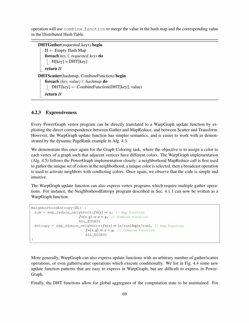
operation will use combine function to merge the value in the hash map and the corresponding valuein the Distributed Hash Table.
DHTGather(requested keys) beginH← Empty Hash Mapforeach key ∈ requested keys do
H[key] = DHT[key]
return H
DHTScatter(hashmap, CombineFunction) beginforeach (key, value) ∈ hashmap do
DHT[key]← CombineFunction(DHT[key], value)
return H
4.2.3 Expressiveness
Every PowerGraph vertex program can be directly translated to a WarpGraph update function by ex-ploiting the direct correspondence between Gather and MapReduce, and between Scatter and Transform.However, the WarpGraph update function has simpler semantics, and is easier to work with as demon-strated by the dynamic PageRank example in Alg. 4.3.
We demonstrate this once again for the Graph Coloring task, where the objective is to assign a color toeach vertex of a graph such that adjacent vertices have different colors. The WarpGraph implementation(Alg. 4.5) follows the PowerGraph implementation closely: a neighborhood MapReduce call is first usedto gather the unique set of colors in the neighborhood, a unique color is selected, then a broadcast operationis used to activate neighbors with conflicting colors. Once again, we observe that the code is simple andintuitive.
The WarpGraph update function can also express vertex programs which require multiple gather opera-tions. For instance, the NeighborhoodEntropy program described in Sec. 4.1.1 can now be written as aWarpGraph function:
NeighborhoodEntropy(Dv) {sum = map_reduce_neighbors(fn(x)⇒ x, // Map Function
fn(x, y)⇒ x+ y, // Combine Function
ALL_EDGES)entropy = map_reduce_neighbors(fn(x)⇒ (x/sum) log(x/sum), // Map Function
fn(x, y)⇒ x+ y, // Combine Function
ALL_EDGES)}
More generally, WarpGraph can also express update functions with an arbitrary number of gather/scatteroperations, or even gather/scatter operations which execute conditionally. We list in Fig. 4.4 some newupdate function patterns that are easy to express in WarpGraph, but are difficult to express in Power-Graph.
Finally, the DHT functions allow for global aggregates of the computation state to be maintained. For
69
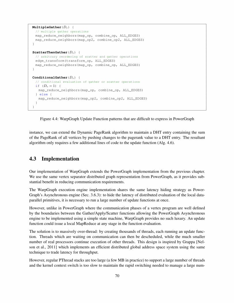
MultipleGather(Dv) {// multiple gather operations
map_reduce_neighbors(map_op, combine_op, ALL_EDGES)map_reduce_neighbors(map_op2, combine_op2, ALL_EDGES)
}
ScatterThenGather(Dv) {// arbitrary reordering of scatter and gather operations
edge_transform(transform_op, ALL_EDGES)map_reduce_neighbors(map_op, combine_op, ALL_EDGES)
}
ConditionalGather(Dv) {// conditional evaluation of gather or scatter operations
if (Dv = 1) {map_reduce_neighbors(map_op, combine_op, ALL_EDGES)
} else {map_reduce_neighbors(map_op2, combine_op2, ALL_EDGES)
}}
Figure 4.4: WarpGraph Update Function patterns that are difficult to express in PowerGraph
instance, we can extend the Dynamic PageRank algorithm to maintain a DHT entry containing the sumof the PageRank of all vertices by pushing changes to the pagerank value to a DHT entry. The resultantalgorithm only requires a few additional lines of code to the update function (Alg. 4.6).
4.3 Implementation
Our implementation of WarpGraph extends the PowerGraph implementation from the previous chapter.We use the same vertex separator distributed graph representation from PowerGraph, as it provides sub-stantial benefit in reducing communication requirements.
The WarpGraph execution engine implementation shares the same latency hiding strategy as Power-Graph’s Asynchronous engine (Sec. 3.6.3): to hide the latency of distributed evaluation of the local data-parallel primitives, it is necessary to run a large number of update functions at once.
However, unlike in PowerGraph where the communication phases of a vertex program are well definedby the boundaries between the Gather/Apply/Scatter functions allowing the PowerGraph Asynchronousengine to be implemented using a simple state machine, WarpGraph provides no such luxury. An updatefunction could issue a local MapReduce at any stage in the function evaluation.
The solution is to massively over-thread: by creating thousands of threads, each running an update func-tion. Threads which are waiting on communication can then be descheduled, while the much smallernumber of real processors continue execution of other threads. This design is inspired by Grappa [Nel-son et al., 2011] which implements an efficient distributed global address space system using the sametechnique to trade latency for throughput.
However, regular PThread stacks are too large (a few MB in practice) to support a large number of threadsand the kernel context switch is too slow to maintain the rapid switching needed to manage a large num-
70
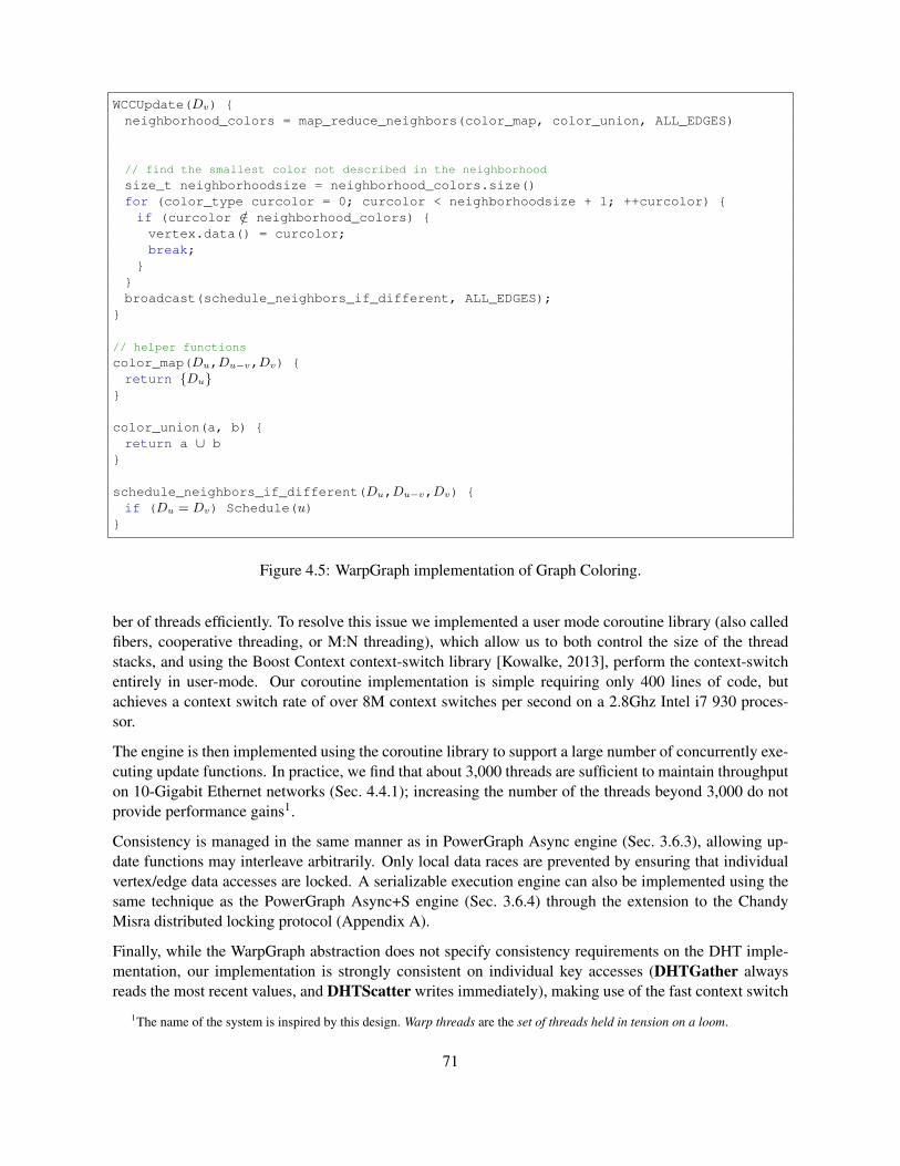
WCCUpdate(Dv) {neighborhood_colors = map_reduce_neighbors(color_map, color_union, ALL_EDGES)
// find the smallest color not described in the neighborhood
size_t neighborhoodsize = neighborhood_colors.size()for (color_type curcolor = 0; curcolor < neighborhoodsize + 1; ++curcolor) {if (curcolor /∈ neighborhood_colors) {vertex.data() = curcolor;break;
}}broadcast(schedule_neighbors_if_different, ALL_EDGES);
}
// helper functions
color_map(Du,Du−v,Dv) {return {Du}
}
color_union(a, b) {return a ∪ b
}
schedule_neighbors_if_different(Du,Du−v,Dv) {if (Du = Dv) Schedule(u)
}
Figure 4.5: WarpGraph implementation of Graph Coloring.
ber of threads efficiently. To resolve this issue we implemented a user mode coroutine library (also calledfibers, cooperative threading, or M:N threading), which allow us to both control the size of the threadstacks, and using the Boost Context context-switch library [Kowalke, 2013], perform the context-switchentirely in user-mode. Our coroutine implementation is simple requiring only 400 lines of code, butachieves a context switch rate of over 8M context switches per second on a 2.8Ghz Intel i7 930 proces-sor.
The engine is then implemented using the coroutine library to support a large number of concurrently exe-cuting update functions. In practice, we find that about 3,000 threads are sufficient to maintain throughputon 10-Gigabit Ethernet networks (Sec. 4.4.1); increasing the number of the threads beyond 3,000 do notprovide performance gains1.
Consistency is managed in the same manner as in PowerGraph Async engine (Sec. 3.6.3), allowing up-date functions may interleave arbitrarily. Only local data races are prevented by ensuring that individualvertex/edge data accesses are locked. A serializable execution engine can also be implemented using thesame technique as the PowerGraph Async+S engine (Sec. 3.6.4) through the extension to the ChandyMisra distributed locking protocol (Appendix A).
Finally, while the WarpGraph abstraction does not specify consistency requirements on the DHT imple-mentation, our implementation is strongly consistent on individual key accesses (DHTGather alwaysreads the most recent values, and DHTScatter writes immediately), making use of the fast context switch
1The name of the system is inspired by this design. Warp threads are the set of threads held in tension on a loom.
71
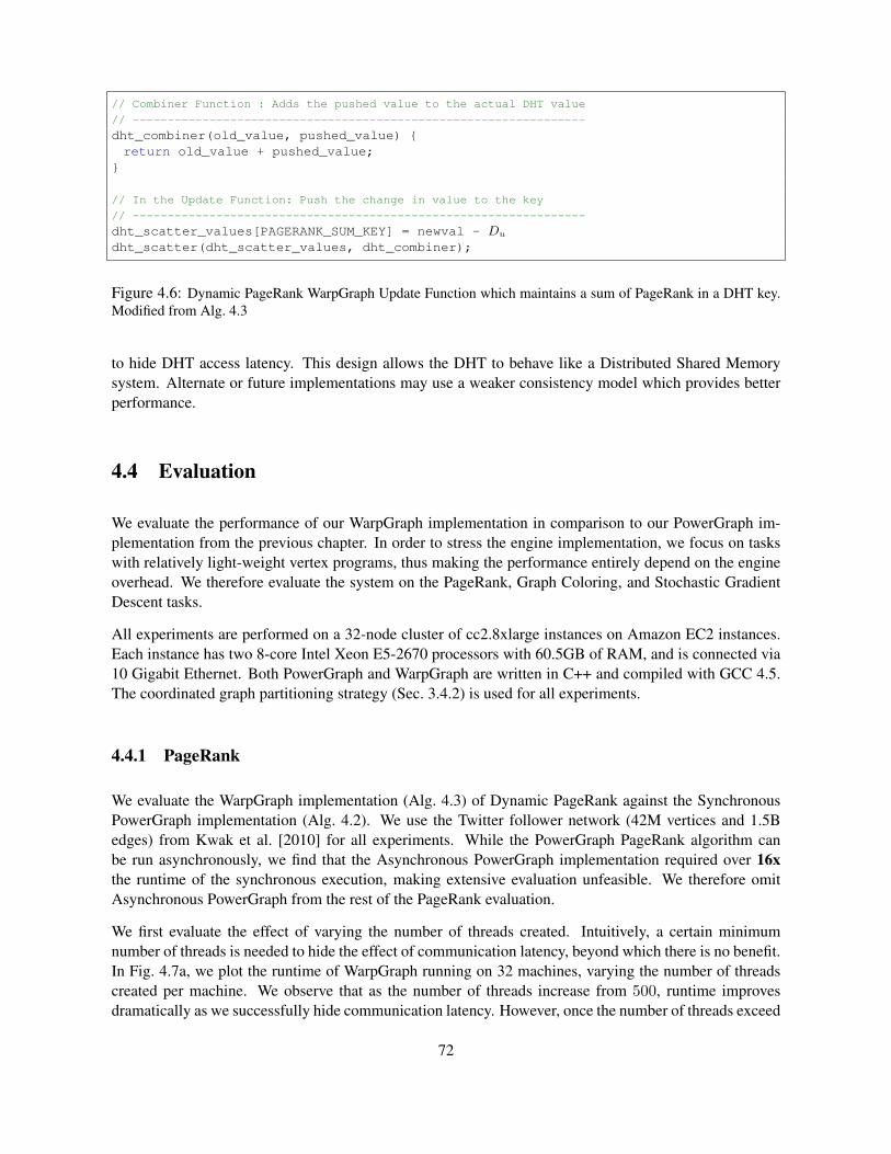
// Combiner Function : Adds the pushed value to the actual DHT value
// -----------------------------------------------------------------
dht_combiner(old_value, pushed_value) {return old_value + pushed_value;
}
// In the Update Function: Push the change in value to the key
// -----------------------------------------------------------------
dht_scatter_values[PAGERANK_SUM_KEY] = newval - Du
dht_scatter(dht_scatter_values, dht_combiner);
Figure 4.6: Dynamic PageRank WarpGraph Update Function which maintains a sum of PageRank in a DHT key.Modified from Alg. 4.3
to hide DHT access latency. This design allows the DHT to behave like a Distributed Shared Memorysystem. Alternate or future implementations may use a weaker consistency model which provides betterperformance.
4.4 Evaluation
We evaluate the performance of our WarpGraph implementation in comparison to our PowerGraph im-plementation from the previous chapter. In order to stress the engine implementation, we focus on taskswith relatively light-weight vertex programs, thus making the performance entirely depend on the engineoverhead. We therefore evaluate the system on the PageRank, Graph Coloring, and Stochastic GradientDescent tasks.
All experiments are performed on a 32-node cluster of cc2.8xlarge instances on Amazon EC2 instances.Each instance has two 8-core Intel Xeon E5-2670 processors with 60.5GB of RAM, and is connected via10 Gigabit Ethernet. Both PowerGraph and WarpGraph are written in C++ and compiled with GCC 4.5.The coordinated graph partitioning strategy (Sec. 3.4.2) is used for all experiments.
4.4.1 PageRank
We evaluate the WarpGraph implementation (Alg. 4.3) of Dynamic PageRank against the SynchronousPowerGraph implementation (Alg. 4.2). We use the Twitter follower network (42M vertices and 1.5Bedges) from Kwak et al. [2010] for all experiments. While the PowerGraph PageRank algorithm canbe run asynchronously, we find that the Asynchronous PowerGraph implementation required over 16xthe runtime of the synchronous execution, making extensive evaluation unfeasible. We therefore omitAsynchronous PowerGraph from the rest of the PageRank evaluation.
We first evaluate the effect of varying the number of threads created. Intuitively, a certain minimumnumber of threads is needed to hide the effect of communication latency, beyond which there is no benefit.In Fig. 4.7a, we plot the runtime of WarpGraph running on 32 machines, varying the number of threadscreated per machine. We observe that as the number of threads increase from 500, runtime improvesdramatically as we successfully hide communication latency. However, once the number of threads exceed
72
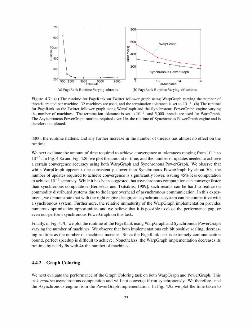
500 1500 3000 5000 7000200
300
400
500
600
700
#Threads
Run
time(
s)
(a) PageRank Runtime Varying #threads
8 16 24 320
200
400
600
800
#Machines
Run
time(
s)
WarpGraph
Synchronous PowerGraph
(b) PageRank Runtime Varying #Machines
Figure 4.7: (a) The runtime for PageRank on Twitter follower graph using WarpGraph varying the number ofthreads created per machine. 32 machines are used, and the termination tolerance is set to 10−3. (b) The runtimefor PageRank on the Twitter follower graph using WarpGraph and the Synchronous PowerGraph engine varyingthe number of machines. The termination tolerance is set to 10−3, and 5,000 threads are used for WarpGraph.The Asynchronous PowerGraph runtime required over 16x the runtime of Synchronous PowerGraph engine and istherefore not plotted.
3000, the runtime flattens, and any further increase in the number of threads has almost no effect on theruntime.
We next evaluate the amount of time required to achieve convergence at tolerances ranging from 10−1 to10−5. In Fig. 4.8a and Fig. 4.8b we plot the amount of time, and the number of updates needed to achievea certain convergence accuracy using both WarpGraph and Synchronous PowerGraph. We observe thatwhile WarpGraph appears to be consistently slower than Synchronous PowerGraph by about 50s, thenumber of updates required to achieve convergence is significantly lower, issuing 45% less computationto achieve 10−5 accuracy. While it has been suggested that asynchronous computation can converge fasterthan synchronous computation [Bertsekas and Tsitsiklis, 1989], such results can be hard to realize oncommodity distributed systems due to the larger overhead of asynchronous communication. In this exper-iment, we demonstrate that with the right engine design, an asynchronous system can be competitive witha synchronous system. Furthermore, the relative immaturity of the WarpGraph implementation providesnumerous optimization opportunities and we believe that it is possible to close the performance gap, oreven out-perform synchronous PowerGraph on this task.
Finally, in Fig. 4.7b, we plot the runtime of the PageRank using WarpGraph and Synchronous PowerGraphvarying the number of machines. We observe that both implementations exhibit positive scaling; decreas-ing runtime as the number of machines increase. Since the PageRank task is extremely communicationbound, perfect speedup is difficult to achieve. Nonetheless, the WarpGraph implementation decreases itsruntime by nearly 3x with 4x the number of machines.
4.4.2 Graph Coloring
We next evaluate the performance of the Graph Coloring task on both WarpGraph and PowerGraph. Thistask requires asynchronous computation and will not converge if run synchronously. We therefore usedthe Asynchronous engine from the PowerGraph implementation. In Fig. 4.9a we plot the time taken to
73
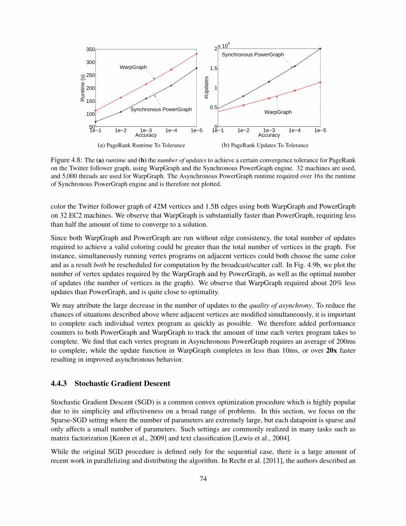
1e−1 1e−2 1e−3 1e−4 1e−550
100
150
200
250
300
350
Accuracy
Run
time
(s)
WarpGraph
Synchronous PowerGraph
(a) PageRank Runtime To Tolerance
1e−1 1e−2 1e−3 1e−4 1e−50
0.5
1
1.5
2x 10⁹
Accuracy
#Upd
ates
WarpGraph
Synchronous PowerGraph
(b) PageRank Updates To Tolerance
Figure 4.8: The (a) runtime and (b) the number of updates to achieve a certain convergence tolerance for PageRankon the Twitter follower graph, using WarpGraph and the Synchronous PowerGraph engine. 32 machines are used,and 5,000 threads are used for WarpGraph. The Asynchronous PowerGraph runtime required over 16x the runtimeof Synchronous PowerGraph engine and is therefore not plotted.
color the Twitter follower graph of 42M vertices and 1.5B edges using both WarpGraph and PowerGraphon 32 EC2 machines. We observe that WarpGraph is substantially faster than PowerGraph, requiring lessthan half the amount of time to converge to a solution.
Since both WarpGraph and PowerGraph are run without edge consistency, the total number of updatesrequired to achieve a valid coloring could be greater than the total number of vertices in the graph. Forinstance, simultaneously running vertex programs on adjacent vertices could both choose the same colorand as a result both be rescheduled for computation by the broadcast/scatter call. In Fig. 4.9b, we plot thenumber of vertex updates required by the WarpGraph and by PowerGraph, as well as the optimal numberof updates (the number of vertices in the graph). We observe that WarpGraph required about 20% lessupdates than PowerGraph, and is quite close to optimality.
We may attribute the large decrease in the number of updates to the quality of asynchrony. To reduce thechances of situations described above where adjacent vertices are modified simultaneously, it is importantto complete each individual vertex program as quickly as possible. We therefore added performancecounters to both PowerGraph and WarpGraph to track the amount of time each vertex program takes tocomplete. We find that each vertex program in Asynchronous PowerGraph requires an average of 200msto complete, while the update function in WarpGraph completes in less than 10ms, or over 20x fasterresulting in improved asynchronous behavior.
4.4.3 Stochastic Gradient Descent
Stochastic Gradient Descent (SGD) is a common convex optimization procedure which is highly populardue to its simplicity and effectiveness on a broad range of problems. In this section, we focus on theSparse-SGD setting where the number of parameters are extremely large, but each datapoint is sparse andonly affects a small number of parameters. Such settings are commonly realized in many tasks such asmatrix factorization [Koren et al., 2009] and text classification [Lewis et al., 2004].
While the original SGD procedure is defined only for the sequential case, there is a large amount ofrecent work in parallelizing and distributing the algorithm. In Recht et al. [2011], the authors described an
74
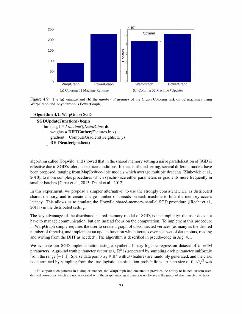
WarpGraph PowerGraph0
50
100
150
200
250
(a) Coloring 32 Machine Runtime
WarpGraph PowerGraph0
1
2
3
4
5
x 107
Upd
ates
Optimal
(b) Coloring 32 Machine #Updates
Figure 4.9: The (a) runtime and (b) the number of updates of the Graph Coloring task on 32 machines usingWarpGraph and Asynchronous PowerGraph.
Algorithm 4.1: WarpGraph SGD
SGDUpdateFunction() beginfor (x, y) ∈ FractionOfDataPoints do
weights = DHTGather(Features in x)gradient = ComputeGradient(weights, x, y)DHTScatter(gradient)
algorithm called Hogwild, and showed that in the shared memory setting a naive parallelization of SGD iseffective due to SGD’s tolerance to race conditions. In the distributed setting, several different models havebeen proposed, ranging from MapReduce-able models which average multiple descents [Zinkevich et al.,2010], to more complex procedures which synchronize either parameters or gradients more frequently insmaller batches [Cipar et al., 2013, Dekel et al., 2012].
In this experiment, we propose a simpler alternative: to use the strongly consistent DHT as distributedshared memory, and to create a large number of threads on each machine to hide the memory accesslatency. This allows us to emulate the Hogwild shared-memory-parallel SGD procedure ([Recht et al.,2011]) in the distributed setting.
The key advantage of the distributed shared memory model of SGD, is its simplicity: the user does nothave to manage communication, but can instead focus on the computation. To implement this procedurein WarpGraph simply requires the user to create a graph of disconnected vertices (as many as the desirednumber of threads), and implement an update function which iterates over a subset of data points, readingand writing from the DHT as needed2. The algorithm is described in pseudo-code in Alg. 4.1.
We evaluate our SGD implementation using a synthetic binary logistic regression dataset of k =1Mparameters. A ground truth parameter vector w ∈ Rk is generated by sampling each parameter uniformlyfrom the range [−1, 1]. Sparse data points xi ∈ Rk with 50 features are randomly generated, and the classis determined by sampling from the true logistic classification probabilities. A step size of 0.2/
√t was
2To support such patterns in a simpler manner, the WarpGraph implementation provides the ability to launch custom user-defined coroutines which are not associated with the graph, making it unnecessary to create the graph of disconnected vertices.
75
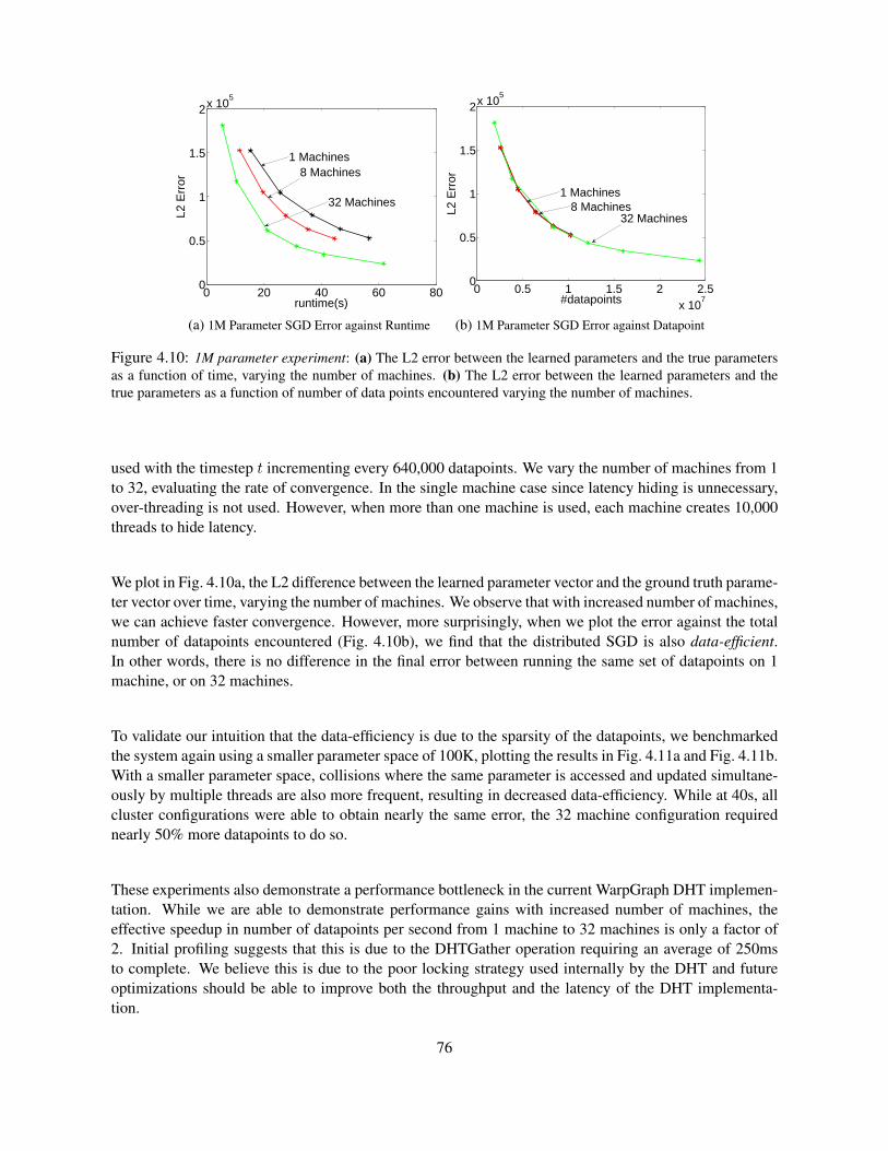
0 20 40 60 800
0.5
1
1.5
2x 10⁵
runtime(s)
L2 E
rror
1 Machines8 Machines
32 Machines
(a) 1M Parameter SGD Error against Runtime
0 0.5 1 1.5 2 2.5x 10
7
0
0.5
1
1.5
2x 10⁵
#datapoints
L2 E
rror
32 Machines
1 Machines8 Machines
(b) 1M Parameter SGD Error against Datapoint
Figure 4.10: 1M parameter experiment: (a) The L2 error between the learned parameters and the true parametersas a function of time, varying the number of machines. (b) The L2 error between the learned parameters and thetrue parameters as a function of number of data points encountered varying the number of machines.
used with the timestep t incrementing every 640,000 datapoints. We vary the number of machines from 1to 32, evaluating the rate of convergence. In the single machine case since latency hiding is unnecessary,over-threading is not used. However, when more than one machine is used, each machine creates 10,000threads to hide latency.
We plot in Fig. 4.10a, the L2 difference between the learned parameter vector and the ground truth parame-ter vector over time, varying the number of machines. We observe that with increased number of machines,we can achieve faster convergence. However, more surprisingly, when we plot the error against the totalnumber of datapoints encountered (Fig. 4.10b), we find that the distributed SGD is also data-efficient.In other words, there is no difference in the final error between running the same set of datapoints on 1machine, or on 32 machines.
To validate our intuition that the data-efficiency is due to the sparsity of the datapoints, we benchmarkedthe system again using a smaller parameter space of 100K, plotting the results in Fig. 4.11a and Fig. 4.11b.With a smaller parameter space, collisions where the same parameter is accessed and updated simultane-ously by multiple threads are also more frequent, resulting in decreased data-efficiency. While at 40s, allcluster configurations were able to obtain nearly the same error, the 32 machine configuration requirednearly 50% more datapoints to do so.
These experiments also demonstrate a performance bottleneck in the current WarpGraph DHT implemen-tation. While we are able to demonstrate performance gains with increased number of machines, theeffective speedup in number of datapoints per second from 1 machine to 32 machines is only a factor of2. Initial profiling suggests that this is due to the DHTGather operation requiring an average of 250msto complete. We believe this is due to the poor locking strategy used internally by the DHT and futureoptimizations should be able to improve both the throughput and the latency of the DHT implementa-tion.
76
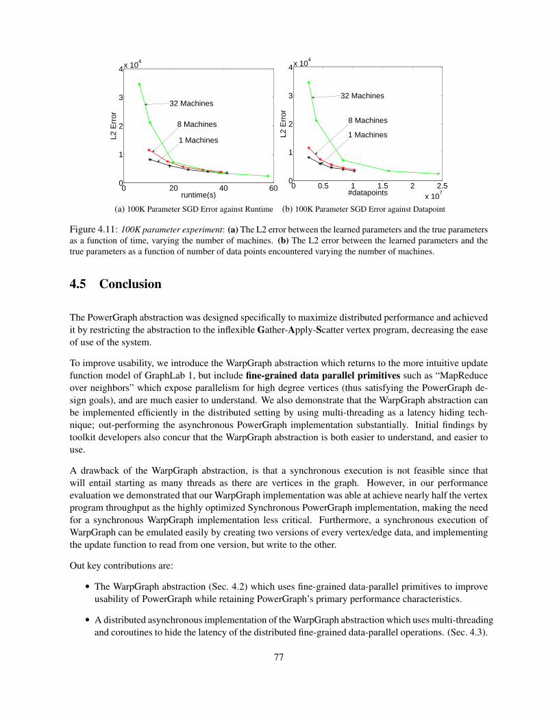
0 20 40 600
1
2
3
4x 10⁴
runtime(s)
L2 E
rror
32 Machines
8 Machines
1 Machines
(a) 100K Parameter SGD Error against Runtime
0 0.5 1 1.5 2 2.5x 10
7
0
1
2
3
4x 10⁴
#datapoints
L2 E
rror
32 Machines
8 Machines
1 Machines
(b) 100K Parameter SGD Error against Datapoint
Figure 4.11: 100K parameter experiment: (a) The L2 error between the learned parameters and the true parametersas a function of time, varying the number of machines. (b) The L2 error between the learned parameters and thetrue parameters as a function of number of data points encountered varying the number of machines.
4.5 Conclusion
The PowerGraph abstraction was designed specifically to maximize distributed performance and achievedit by restricting the abstraction to the inflexible Gather-Apply-Scatter vertex program, decreasing the easeof use of the system.
To improve usability, we introduce the WarpGraph abstraction which returns to the more intuitive updatefunction model of GraphLab 1, but include fine-grained data parallel primitives such as “MapReduceover neighbors” which expose parallelism for high degree vertices (thus satisfying the PowerGraph de-sign goals), and are much easier to understand. We also demonstrate that the WarpGraph abstraction canbe implemented efficiently in the distributed setting by using multi-threading as a latency hiding tech-nique; out-performing the asynchronous PowerGraph implementation substantially. Initial findings bytoolkit developers also concur that the WarpGraph abstraction is both easier to understand, and easier touse.
A drawback of the WarpGraph abstraction, is that a synchronous execution is not feasible since thatwill entail starting as many threads as there are vertices in the graph. However, in our performanceevaluation we demonstrated that our WarpGraph implementation was able at achieve nearly half the vertexprogram throughput as the highly optimized Synchronous PowerGraph implementation, making the needfor a synchronous WarpGraph implementation less critical. Furthermore, a synchronous execution ofWarpGraph can be emulated easily by creating two versions of every vertex/edge data, and implementingthe update function to read from one version, but write to the other.
Out key contributions are:
• The WarpGraph abstraction (Sec. 4.2) which uses fine-grained data-parallel primitives to improveusability of PowerGraph while retaining PowerGraph’s primary performance characteristics.
• A distributed asynchronous implementation of the WarpGraph abstraction which uses multi-threadingand coroutines to hide the latency of the distributed fine-grained data-parallel operations. (Sec. 4.3).
77
• An evaluation of the WarpGraph implementation, demonstrating that our WarpGraph design sub-stantially out-perform the Asynchronous PowerGraph implementation, and can approach the per-formance of the Synchronous PowerGraph implementation. (Sec. 4.4)
78
Chapter 5
Related Work
There are several historical, or existing frameworks which can be used for parallel ML. We address thedifferences between GraphLab and these other abstractions here.
5.1 Map-Reduce Abstraction
A program implemented in the MapReduce framework consists of a Map operation and a Reduce oper-ation. The Map operation is a function which is applied independently and in parallel to each datum (e.g.,webpage) in a large data set (e.g., computing the word-count). The Reduce operation is an aggregationfunction which combines the Map outputs (e.g., computing the total word count). MapReduce performsoptimally only when the algorithm is embarrassingly parallel and can be decomposed into a large numberof independent computations. The MapReduce framework expresses the class of ML algorithms which fitthe Statistical-Query model [Chu et al., 2007] as well as problems where feature extraction dominates therun-time.
The MapReduce abstraction fails when there are computational dependencies in the data. For example,MapReduce can be used to extract features from a massive collection of images but cannot representcomputation that depends on small overlapping subsets of images. This limitation makes it difficult torepresent algorithms that operate on structured models. As a consequence, when confronted with largescale problems, we often abandon rich structured models in favor of simpler methods that are amenableto the MapReduce abstraction.
Furthermore, many ML algorithms iteratively transform parameters during both learning and inference.For example, algorithms like Belief Propagation (BP), EM, gradient descent, and even Gibbs sampling,iteratively refine a set of parameters until some termination condition is achieved. While the MapReduceabstraction can be invoked iteratively, it does not provide a mechanism to directly encode iterative com-putation. As a consequence, it is not possible to express sophisticated scheduling, automatically assesstermination, or even leverage basic data persistence.
The popular implementations of the MapReduce abstraction are targeted at large data-center applicationsand therefore optimized to address node-failure and disk-centric parallelism. The overhead associatedwith the fault-tolerant, disk-centric approach is unnecessarily costly when applied to the typical clusterand multi-core settings encountered in ML research. Nonetheless, MapReduce is used in small clusters
79
and even multi-core settings [Chu et al., 2007]. The GraphLab implementations do not address fault-tolerance or parallel disk access and instead assumes that processors do not fail and all data is stored inmemory. While this provides a massive performance advantage, it limits the implementation to datasetsizes which can fit in distributed memory. The GraphLab abstraction however, does not prescribe norrequire the in-memory model, and [Kyrola et al., 2012] has demonstrated that it is possible to implementGraphLab on disk without much loss in performance.
5.1.1 Relation to GraphLab
MapReduce may be used to execute one synchronous iteration of GraphLab 1 by mapping over everyvertex and edge, and computing the entire update function in the Reducer. Iterative computation can thenbe defined through the use of either explicit MapReduce calls, or iterative MapReduce methods [Bu et al.,2010, Ekanayake et al., 2010]. Dynamic execution and asynchronous execution however, are difficult totranslate.
PowerGraph’s Gather-Apply-Scatter model factorizes the computation over edges, and uses the vertex-separator partitioning to minimize communication. A similar strategy can also be used to optimize theMapReduce execution. Given an edge-list graph representation where each row of the input file containsthe edge data on the edge as well as the vertex data of both endpoints, the Gather operation can be emulatedthrough the use of Combiners. This allows MapReduce to achieve the communication reduction observedby PowerGraph. Finally, the Apply phase can be executed on the Reducers, and the Scatter phase can beexecuted with another MapReduce pass.
The WarpGraph model however, due to its generality is difficult to emulate in MapReduce. While Warp-Graph update functions which perform the same sequence of operation on all vertices can be compiledinto a fixed sequence of MapReduce operations, other cases such as conditional gathers (Fig. 4.4) wherethe choice of aggregation operation is data-dependent, are difficult to emulate.
The key performance limitation with translating GraphLab programs to MapReduce is due to the re-quirement that every Mapper is independent. To execute graph algorithms in MapReduce, thus leads tounnecessary replication of information, which in some cases can lead to an asymptotic increase in com-munication and storage requirements (Sec. 3.6.6).
In the reverse direction, MapReduce can be emulated efficiently in all GraphLab abstractions by treatingthe data graph as a dataflow graph. By constructing a fully connected bipartite graph with one set ofvertices representing Mappers, the other set of vertices representing Reducers, and using the edges forcommunication, we can achieve a communication efficient emulation of MapReduce. The limitationhowever, lies in the GraphLab implementations which require all data to fit in memory.
5.2 BSP Abstraction (Pregel)
The question of how the GraphLab abstractions compare with the Pregel [Malewicz et al., 2010] ab-straction is often raised since both systems emerged at nearly the same time as solutions for large graphcomputation1. Due to the similarities in design goals between GraphLab and Pregel, we provide here amore exhaustive analysis of the abstraction differences.
1A description of the Pregel abstraction is provided in Sec. 2.1.
80
5.2.1 Dynamic Execution
While Pregel also supports dynamic execution in that only vertices which receive messages will be exe-cuted; there is a crucial difference between how dynamic execution behaves in a Message Passing abstrac-tion such as Pregel, and a (restricted) shared memory abstraction such as GraphLab.
In Pregel, when a vertex is executed, it is unable to read its neighboring vertex/edge data, and insteadmust rely upon its neighbors sending it the necessary state. For instance, the dynamic PageRank algorithmdescribed in Alg. 2.1 cannot be easily implemented within Pregel; while you can signal a vertex to executein the next round via a message, the signaled vertex is unable to recompute its own value since it cannotread its neighbors information.
5.2.2 Asynchronous Computation
The Gibbs Sampling [Geman and Geman, 1984] process is conceptually simple, each vertex in the graphrepresents a single variable in a probability distribution. Computation then proceeds in the sequential caseby picking a vertex, and drawing a sampling from the distribution of the vertex condition on the values ofits neighboring vertices. Unfortunately in the parallel case, performing this update on all vertices simul-taneously will not converge to a meaningful answer [Gonzalez et al., 2011, Siapas, 1996]. Asynchronouscomputation with edge consistency is necessary to guarantee convergence; though empirically in manysettings weaker consistency is sufficient.
All versions of GraphLab provide asynchronous computation capabilities, with optionally enforced edgeconsistency; implemented either through locking (Sec. 2.3.1, Sec. 2.4.2.2, Sec. 3.6.4, Sec. 4.3), or specificengine choices (Sec. 2.4.2.1).
On the other hand, Gibbs Sampling is difficult to express in Pregel since any given vertex cannot unilater-ally choose to read the values on neighboring vertices. The asynchronous computation necessary is alsodifficult to express. While the chromatic engine could conceptually be implemented in the Pregel, a largeamount of additional coordination is necessary.
5.2.3 Edge Data
The GraphLab abstractions include the notion of persistent and mutable edge data, which is useful is manysettings:
1. To contain the “messages” in message-passing graphical model inference procedures such as beliefpropagation. (Sec. 2.3.3.1, Sec. 2.4.4.2)
2. In matrix factorization for collaborative filtering to store the current predicted rating for a user-movie pair. (Sec. 2.4.4.1)
3. In some graph algorithms such as triangle counting to maintain the number of triangles passingthrough each edge.
4. In Latent Dirichlet Allocation [Blei et al., 2003] where a graph is constructed between documentsand words, to contain the sampled topics for each word occurrence.
81
Without edge data, Pregel must store the edge state on the vertices of the graph which incurs unnecessaryreplication in the common event that both ends of the edge needs access to the edge data.
5.2.4 Generalized Messaging
Pregel, while frequently described as being restricted to communication along edges of a graph, doestechnically permit messaging of arbitrary vertex programs from any other vertex program. The “graph” istherefore largely a user construct, and the abstraction permits a more general programming model similarto generalized BSP message passing [Skillicorn et al., 1997].
GraphLab however, enforces all communication patterns between vertex programs to be strictly limited tothe graph structure. The only deviations permitted are through the Sync operation (Sec. 2.2.5) in GraphLaband PowerGraph, and the DHT (Sec. 4.2.2.4) in WarpGraph, both of which provide no guarantees ofconsistency nor recency of data.
5.2.5 Scatter vs Gather
GraphLab provides an efficient distributed representation of algorithms where update functions needs datafrom adjacent vertices. For instance, consider the alternative least squares (ALS) problem for Netflix ma-trix factorization. ALS in GraphLab involves simply representing the graph as a bipartite graph betweenusers and movies. For each movie a user rents, an edge between the user and the corresponding movie iscreating containing the user rating for the movie. ALS then proceeds in an asynchronous fashion: for eachuser, update the user vector to better predict the user ratings while holding all the movie vectors fixed.This is then repeated for each movie and the whole process loops until convergence is obtained.
To implement ALS in Hadoop, the Map-function does essentially no computational work and instead onlyemits copies of the vertex data for every edge in the graph. For example, a user vertex which connectsto 100 movies must emit the data on the user vertex 100 times, once for each movie. This results in thegeneration of a large amount of unnecessary network traffic and unnecessary HDFS writes. This weaknessextends beyond the MapReduce abstraction, but also affects the graph message-passing models (such asPregel) due to the lack of a defined scatter operation which would avoid sending same value multipletimes to each machine. Comparatively, the GraphLab abstractions are simpler as users do not need toexplicitly define the flow of information. Synchronization of a modified vertex will only communicate themodifications to machines which require the vertex data for computation.
On the other hand, most other frameworks have very efficient gather operations. Piccolo [Power and Li,2010], Pregel [Malewicz et al., 2010] provide efficient combiner operations which allow messages goingto the same vertex to be “pre-combined” on the source machine, thus minimizing network communication.While GraphLab lacks such a gather operation, PowerGraph and WarpGraph resolves this limitation byexplicitly specifying a gather operation.
PowerGraph and WarpGraph are, as far as the author is aware, the only high level abstraction whichefficiently represents both gather and scatter capabilities.
82
5.2.6 Relation to GraphLab
GraphLab 1 can be emulated in Pregel by simply having each vertex broadcast its value to all neighborsproviding every vertex with the complete scope information in the next super-step. PowerGraph’s gatheroperation can be emulated through the use of message combiners, and the scatter operation can be em-ulated simply through the use of messages. However as mentioned in the subsections above, the scatteremulation is inefficient. Furthermore, Pregel cannot express the same dynamic execution (Sec. 5.2.1) andasynchronous (Sec. 5.2.2) execution semantics as GraphLab or PowerGraph.
Finally, just like MapReduce, while a restricted class of WarpGraph update functions which perform thesame sequence of operation on all vertices can be compiled into Pregel, other cases such as conditionalgathers (Fig. 4.4) where the choice of aggregation operation is data-dependent, are difficult to emulate;possibly requiring large state machines on each vertex.
Pregel however, can be emulated efficiently in all GraphLab abstractions by using the graph edges to storecommunicated messages. Furthermore, the PowerGraph and WarpGraph abstractions can further optimizePregel programs by providing an efficient broadcast primitive.
5.3 Generalized SpMV Abstraction
The generalized sparse matrix vector product (SpMV) abstraction [Buluc and Gilbert, 2011, Kang et al.,2009] expresses computation as multiplication between large sparse matrices and dense vectors wherethe data types used in the matrix and vector entries are user-defined with arbitrary multiply and sumoperations. This can be seen as a constrained version of the PowerGraph’s Gather operation. Just like theBSP Abstraction, the SpMV abstraction cannot effectively expose dynamic, asynchronous computation,and only efficiently defines gather operations but not scatter operations.
5.3.1 Relation to GraphLab
The SpMV abstractions lack a notion of mutable edge data, thus can make GraphLab programs whichrequire edge data difficult to express. Furthermore, the current SpMV abstractions lack both dynamic andasynchronous computation capabilities. On the other hand, since the SpMV abstraction is a special caseof PowerGraph’s Gather operation, it can be emulated in PowerGraph efficiently.
5.4 Dataflow Abstraction
In the Dataflow abstraction, parallel computation is represented as a directed acyclic graph with dataflowing along edges between vertices. Vertices correspond to functions which receive information oninbound edges and output results to outbound edges. Implementations of this abstraction include Dryad[Isard et al., 2007], Pig Latin [Olston et al., 2008] and Spark [Zaharia et al., 2010].
While the DAG abstraction permits rich computational dependencies, it can only express synchronousiterative computation. Dynamic computation or asynchronous computation cannot be expressed.
83
5.4.1 Relation to GraphLab
The generality of the dataflow abstractions can permit efficient implementations of the GraphLab andPowerGraph execution models [Xin et al., 2013]. However, WarpGraph relies on fine-grained aggrega-tion primitives and only a restricted subset of update functions can potentially be compiled into a coarsedataflow execution. Update functions which require conditional gathers (Fig. 4.4) where the choice ofaggregation operation is data-dependent, are difficult to emulate.
Dataflow abstractions can be emulated efficiently in GraphLab by using the dataflow graph as the datagraph, and using edges for communication. However the GraphLab abstractions do not, natively, providethe advantages of the dataflow abstractions such as fault-tolerance, streaming computation, and the use ofthe datasets larger than memory requirements. Building such capabilities into the GraphLab abstractionsrequire much greater complexity.
5.5 Datalog/Bloom
Datalog is a powerful declarative logic programming language that has been extended by Bloom [Alvaroet al., 2011] to distributed environments, leading to a rich abstraction for distributed asynchronous sys-tems. More recently, Datalog/Bloom has been shown to be useful for understanding certain classes ofasynchronous fixed point computation [Conway et al., 2012], as well as incremental computation [McSh-erry et al., 2013].
Datalog/Bloom is unlike MapReduce, Pregel and other dataflow abstractions in that Datalog does notprescribe a specific execution strategy. The Datalog/Bloom programmer instead simply specifies relation-ships between facts, and it is up to the implementation/query optimizer to figure out the most efficientexecution strategy. As a result, Datalog/Bloom has an interesting similarity with GraphLab where theuser simply defines a vertex program describing the evolution of graph data, then different engine imple-mentations/scheduler strategies may be used to execute the program to convergence. Understanding thisrelationship has great potential for interesting future work. Some intriguing possibilities include embed-ding Datalog/Bloom as a high-level domain specific language for GraphLab, or using some of GraphLab’slarge-graph partitioning strategies to accelerate program execution in Datalog/Bloom.
84
Chapter 6
Conclusion
6.1 Thesis Summary
As the people gets more interconnected through the Internet, and as data collection capabilities increase,we enter a new era of Big Data where companies collect and store more information than they can use.As a result, Machine Learning methods become increasingly important as a means of extracting andsummarizing useful information from large quantities of data. Google, with its PageRank algorithm (andother proprietary ad-targeting algorithms), as well as Netflix with the success of the Netflix competition,have demonstrated the usefulness and importance of Machine Learning for tech companies.
To apply Machine Learning methods to massive datasets as frequently encountered in the real world,use of parallelism and large scale distributed computation is necessary. However, since programming fordistributed systems is highly challenging, the use of high level abstractions such as MapReduce, Dryadand Pregel are often used, which hide much of the complexity. In this thesis, we identified that such highlevel abstractions, while suitable for a broad range of data processing tasks, do not fit the needs of MachineLearning algorithms. Specifically, in Sec. 1.1.1 we identified four key aspects:
Interdependent Computation Many ML algorithms do not treat data points as independent quantities,but can exploit relationships between data to extract deep and interesting signals.
Asynchronous Iterative Computation ML algorithms are iterative in nature, executing the same se-quence of computation repeatedly. Furthermore many algorithms are asynchronous in nature; re-quiring the most recent parameter values for each computation.
Dynamic Computation Parameters may not converge uniformly in iterative ML algorithms. Focusingcomputation on difficult regions of the computation can provide performance gains.
Serializability/Sequential Consistency A serializable execution is beneficial for debugging, and cer-tain algorithms such as Gibbs Sampling require it for correctness. However, as we suggested inSec. 3.1.3, newer empirical results have suggested that ML algorithms may be tolerant to serializability-breaking execution.
Existing computation abstractions such as MapReduce and Pregel are unable to express the Dynamic,Asynchronous, Iterative computation common to many ML algorithms. While in some cases it is possible
85
to coerce an algorithm into a mismatched abstraction, a large efficiency penalty must be paid. As such,we propose a new abstraction called GraphLab, designed to explicitly expose these properties.
In Chap. 2, we defined the GraphLab 1 abstraction, which consists of a data graph where arbitrary datamay be stored on vertices and edges; an update function/vertex program which describes local compu-tation on vertices; and a scheduler which determines the order of update functions executed. Additionally,a consistency model is used to determine the extent at which computation may overlap and hence race.Finally, a Sync mechanism is used to provide global state when necessary. We implemented the abstrac-tion in both the shared memory and distributed memory setting and demonstrated the expressiveness,usefulness and performance that can be obtained through the use of a domain specific abstraction.
While the distributed system built in Chap. 2 works well for regular graphs of over 100 million verticesand edges, it fails on real-world graphs with power-law degree distributions containing billions of verticesand edges. To scale to such problems, in Chap. 3 we introduced PowerGraph which restricts the generalupdate function model in GraphLab 1 to the GAS: Gather-Apply-Scatter structure. The GAS model ofthe vertex program allowed individual vertex program to be parallelized, improving performance on highdegree vertices; and also allowed the use of the vertex-separator model for distributed graph represen-tation, bringing about large reductions in communication and storage requirements. We also introducednew streaming graph partitioning heuristics to improve graph partitioning quality. Our distributed im-plementation of PowerGraph achieved state of the art performance, and in some cases, improved overthem by orders of magnitude. Our open source project at http://graphlab.org implements over24 different algorithms and has been downloaded thousands of times.
PowerGraph sacrificed usability for performance; the behavior of the PowerGraph abstraction is difficultto understand, and the Gather-Apply-Scatter restriction makes certain computations difficult to represent,if not impossible. In Chap. 4, we introduce the WarpGraph abstraction to address the usability issue.Through the use of fine-grained data parallel abstractions which allow update functions to call aggregateoperations over its neighborhood, we combine the power of PowerGraph, with the simplicity of GraphLab1. Our implementation relied on the use of cooperative threading: to use thousands of threads to hidecommunication latency. We demonstrated that the WarpGraph abstraction is not just strictly more ex-pressive than PowerGraph, but is also easier to use and understand. Our WarpGraph implementationoutperforms the asynchronous implementations of PowerGraph and is competitive with the synchronousPowerGraph implementation on certain tasks, demonstrating the feasibility of asynchronous computationin the distributed setting.
We summarize the three abstractions we developed in Table 6.1.
6.2 Observations
We learned several key lessons through the development of this thesis.
Importance of Dynamic Computation and Computation Sparsity
As data set sizes increase, batch Machine Learning methods which require multiple complete passes overthe entire dataset become impractical. the use of dynamic computation which focuses computation ondifficult regions of the problem is necessary to maintain performance. Furthermore in the real-world,dataset sizes are not static, but grow incrementally. The ability to focus computation on only the affected
86
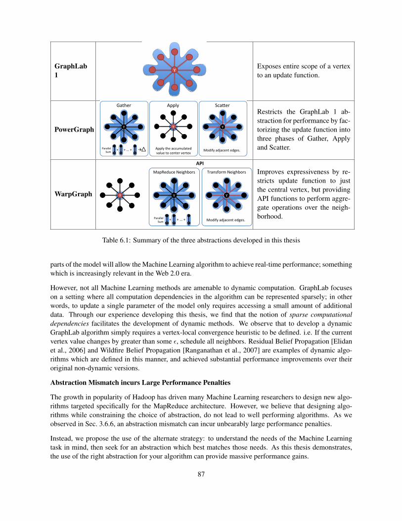
GraphLab1
Y Exposes entire scope of a vertexto an update function.
PowerGraph Y
Apply the accumulated value to center vertex
Apply
Y
Modify adjacent edges.
Sca<er
+ + … + à Δ
Y Y Y
Parallel Sum
Y
Gather Restricts the GraphLab 1 ab-straction for performance by fac-torizing the update function intothree phases of Gather, Applyand Scatter.
WarpGraph Y
API
Y
Modify adjacent edges.
Transform Neighbors
+ + … +
Y Y Y
Parallel Sum
Y
MapReduce Neighbors Improves expressiveness by re-stricts update function to justthe central vertex, but providingAPI functions to perform aggre-gate operations over the neigh-borhood.
Table 6.1: Summary of the three abstractions developed in this thesis
parts of the model will allow the Machine Learning algorithm to achieve real-time performance; somethingwhich is increasingly relevant in the Web 2.0 era.
However, not all Machine Learning methods are amenable to dynamic computation. GraphLab focuseson a setting where all computation dependencies in the algorithm can be represented sparsely; in otherwords, to update a single parameter of the model only requires accessing a small amount of additionaldata. Through our experience developing this thesis, we find that the notion of sparse computationaldependencies facilitates the development of dynamic methods. We observe that to develop a dynamicGraphLab algorithm simply requires a vertex-local convergence heuristic to be defined. i.e. If the currentvertex value changes by greater than some ε, schedule all neighbors. Residual Belief Propagation [Elidanet al., 2006] and Wildfire Belief Propagation [Ranganathan et al., 2007] are examples of dynamic algo-rithms which are defined in this manner, and achieved substantial performance improvements over theiroriginal non-dynamic versions.
Abstraction Mismatch incurs Large Performance Penalties
The growth in popularity of Hadoop has driven many Machine Learning researchers to design new algo-rithms targeted specifically for the MapReduce architecture. However, we believe that designing algo-rithms while constraining the choice of abstraction, do not lead to well performing algorithms. As weobserved in Sec. 3.6.6, an abstraction mismatch can incur unbearably large performance penalties.
Instead, we propose the use of the alternate strategy: to understand the needs of the Machine Learningtask in mind, then seek for an abstraction which best matches those needs. As this thesis demonstrates,the use of the right abstraction for your algorithm can provide massive performance gains.
87
The GraphLab thesis grew out of a similar process. After working on parallel and distributed BeliefPropagation (BP) methods [Gonzalez et al., 2009a,b], we isolated the core computation abstraction needsof BP and discovered that it is sufficiently general to be used for a broad range of ML algorithms. Theoutcome is a high level domain specific abstraction which can be applied to many ML tasks, and does notsacrifice performance.
Every Few Orders of Magnitude of Scaling Requires a Redesign
This statement is a useful design principle to consider when scaling new algorithms, implementations ofML procedures, or computation abstractions to larger real-world datasets. System designs and algorithmswhich work on smaller datasets may completely fail when operating on datasets an order of magnitudelarger; requiring a fundamental rethink of the entire system.
We learned this lesson when attempting to scale GraphLab to real world graphs of billions of vertices andedges. We discovered that the vertex-ghosting procedure does not scale and resulted in excessive repli-cation; and the difficulty of partitioning such large graphs exacerbated the situation. To resolve this issuerequired a fundamental redesign of the GraphLab computation model which resulted in the PowerGraphabstraction.
88
6.3 Future Work
Through the development of this thesis, we encountered several interesting research questions.
6.3.1 Graph Partitioning
Extensive research has been done on computation of high quality edge separators on graphs, but compara-tively little work exist for vertex separators. While the streaming partitioning process described in Chap. 3performed reasonably well, more research into improved streaming vertex separator algorithms will helpimprove performance of the GraphLab platform dramatically.
6.3.2 Incremental Machine Learning
We would like to consider the situation where GraphLab is used to maintain convergence of an opti-mal solution to some optimization procedure while the input graph is under continuous modification.For instance in the Netflix matrix factorization problem, we could use GraphLab to maintain a solutionto the factorization while new users, new movies, or new user-movie rental pairs are continuously in-serted.
The setting bears resemblance to online machine learning [Blum, 1996], but a key difference is that thealgorithm is provided access to all existing data and not just one data element at a time. The setting bearsmuch closer resemblance to incremental optimization as defined in Hartline [2008] (and hence we giveit the same name) though Hartline [2008] analyzed the setting only for particular discrete optimizationproblems such as max-flow and matching. However, key differences still exist in that we allow arbitrarychanges to be made to existing data including modifications of existing data points, and removal of data.Still more related are warm-start optimization techniques such as in Yildirim and Wright [2002] andGondzio and Grothey [2008], where an optimization problem is solved using the solution of a similar orperturbed problem for initialization.
Such a learning system can be built into GraphLab easily by permitting GraphLab to load graphs fromexternal databases. GraphLab is first used to provide a solution to some initial graph. Following which,as data is added or modified, GraphLab’s dynamic scheduling capabilities are used to update the minimalset of vertices to maintain convergence. The key idea is therefore to warm-start a solution to a modifiedproblem, using a solution to the original problem.
A theoretical understanding of how solutions to optimization problems move as data is modified, as wellan understanding of how dynamic scheduling behaves in these problems could lead to efficient methodsto solve with high accuracy, extremely large optimization problems.
6.3.3 Dynamic Execution
As mentioned above in Sec. 6.2, GraphLab provides dynamic execution capabilities which will allow thealgorithm to focus computation on the hardest parts of the problem. The potential performance benefitsthat can be gained from the use of dynamic execution is very large.
89

However, most Machine Learning algorithms are still defined in the strict fully iterative sense: where thesame sequence of operations are executed every round. Additional research has to be done in this area tounderstand how to take advantage of dynamic scheduling in Machine Learning algorithms.
6.3.4 Fault Tolerance
We have empirically observed that some iterative Machine Learning algorithms such as ALS, appear to bestrongly fault tolerant by nature; that upon machine failure and losing a fraction of the learned parameters,simply resetting the lost parameters to reasonable values and resuming the algorithm is sufficient. Only afew additional iterations are needed to bring the error rate to pre-machine-failure values.
We believe that this behavior is related to the warm-start property in many optimization procedures andtherefore ties in strongly with the Incremental Machine Learning research direction described above. Abetter understanding of the inherent fault tolerance properties of Machine Learning algorithms will providegreat benefit to the use of Machine Learning on massive datasets in very large cluster deployments ofthousands of machines.
6.3.5 Other Abstractions
GraphLab is designed to operate well on a reasonably broad family of Machine Learning algorithms;covering a space what we categorize as Sparse Iterative methods. However, the breadth of MachineLearning far exceeds the domain of tasks GraphLab is designed for. GraphLab is not particularly suitablefor:
Dense Iterative Unlike Sparse Iterative methods, Dense Iterative methods involve the manipulation oflarge dense matrices. Kernel methods, even including many low-rank versions fall into this category.
Iterative ParFor This is a generalized form of iterative MapReduce, allowing arbitrary read-only mem-ory sharing between parallel threads. This describes classes of optimization procedures such asLBFGS, Batch Gradient Descent, FISTA, etc. AllReduce [all] is an example of an abstraction forthis category of problems.
Online Learning This describes methods based on streaming data which encounter each datapoint ex-actly once. SGD and Bandit algorithms are examples of algorithms in this category. This categoryalso include streaming and sketching procedures such as the well known Count-Min Sketch forapproximate statistics [Cormode and Muthukrishnan, 2005].
Instance Based Learning This describes procedures such as K-NN, and top-K-inner product which havea simple learning process, but have a complex test time query process.
New models, new abstractions and new algorithms are needed to scale these classes of problems to the BigData setting. A promising new abstraction which emerged in recent years is the Parameter Server whichwe will describe in greater detail.
90
6.3.6 Parameter Server
The Parameter Server model is a form of a weak consistency distributed shared memory architecture. ADistributed Hash Table is used to maintain global parameter information, and machines read and write tothe Distributed Hash Table (DHT) directly in parallel. To obtain performance, several techniques are usedincluding the use of local caching, or requiring that the hash table values form Abelian Group.
First explored in Smola and Narayanamurthy [2010] and generalized in Ahmed et al. [2012], the parameterserver model has found applications in Gibbs Sampling [Ahmed et al., 2011, Low et al., 2011, Smola andNarayanamurthy, 2010], Stochastic Gradient Descent (Sec. 4.4.3), and could potentially be applied forother optimization procedures as well.
While the notion of distributed shared memory is not new, the novelty in the parameter server has beento specialize the weak consistency model for the purposes of Machine Learning. For instance, [Ciparet al., 2013] defined cache staleness to be dependent on the iteration counter of the ML algorithm. Otherpossible staleness conditions are conceivable: based on the frequency of modification of the parameteror the amount of change in the parameter. Or even in Sec. 4.4.3 which does not use a cache but insteademulates massive parallelism to hide the latency of distributed memory.
The parameter server model is convenient since it is highly general, being functionally similar to dis-tributed shared memory. However, more theoretical and empirical work has to be done to understandthe space of algorithms for which the parameter server model is useful; and among the many possiblevariations of the parameter server, which is the best.
91
Appendix A
Extended Chandy Misra
The Dining Philosopher’s problem provides a convenient analogy for the locking procedure needed forGraphLab’s “edge consistency” model (Sec. 2.2.4). Let each edge in the graph represent a fork (we ignoreedge direction), and let each vertex represent a philosopher. Since Each philosopher must pick up allforks on all adjacent edges before he can eat, therefore adjacent philosophers cannot eat simultaneously;satisfying the requirements of Edge Consistency. As a result, any solution to the Dining Philosopher’sproblem, also describes a solution for enforcing edge consistency.
The locking procedure used by the shared memory and distributed memory implementation of GraphLabin Chap. 2, corresponds exactly to the Dijstra solution described in Dijkstra [1971]. However, for largegraphs with high degree vertices, the requirement to acquire locks sequentially, limits performance dra-matically. Furthermore, the overhead of “fair mutex” datastructures, where a queue has to be maintainedper mutex increases memory load substantially in the distributed setting.
Instead, for PowerGraph (Chap. 3), we consider an alternate method based on the the Chandy Misrasolution [Chandy and Misra, 1984].
A.1 Chandy Misra
We will begin by describing the classical Chandy Misra solution to the Dining Philosopher’s problem.
Each Philosopher cycles through the following 3 states.
Thinking Philosopher is inactive. After some time, he may get hungry.
Hungry Philosopher wants to eat and is trying to acquire all adjacent forks. Once all forks are acquired,he begins Eating.
Eating Philosopher has all forks and is eating. After some finite amount of time, he stops eating and goesback to Thinking.
Each edge represents a fork, and thus can only be used by the two philosophers on its endpoints. The forkis always owned by one of its adjacent philosophers and must be in one of two states:
92
Clean The philosopher currently owning the fork keeps the fork even if others request for it. The forkbecomes after the philosopher eats.
Dirty The philosopher currently owning the fork gives up the fork if others request for it. The fork iscleaned when it changes hands.
At initialization all forks are initially dirty, and are owned by the philosopher with the lower ID.
The Chandy Misra algorithm is described by the following pseudocode.
When philosopher v becomes hungry:Send request for each unowned fork adjacent to v
When philosopher v receives request for fork f :if v is Eating or f is clean% v is using the fork. Don’t give it up.Store request
elseif v is Thinking% v is not using the fork. Give it up.Clean Fork f and give up fork
elseif v is Hungry and f is dirty% v wants the fork, but the neighbor has priority since fork is dirty% Give it up, but also request for it so I get it backClean Fork f and give up forkSend request for fork f
end
When philosopher v has all needed forks and is hungry:% v got all the forks. He can eat.Change state of $v$ to Eating
When philosopher v Stops Eating:% Finished eating, so all forks are dirty.Change state of $v$ to Thinking.Set all forks to be Dirty.% Give forks up to everyone who asked for it.for each stored request:Clean the requested fork and give it up
end
Surprisingly, the above procedure will never deadlock and is fair if the initialization of forks is donecorrectly. We refer to the original paper [Chandy and Misra, 1984] for the proof.
A.2 Hierarchical Chandy Misra
While the Chandy Misra algorithm highly natural for the distributed setting since the algorithm is de-scribed in terms of “messages” between philosophers, it only works for the distributed edge-separatorsetting where the partitioning is defined by placing philosophers on machines.
In the vertex-separator setting (Chap. 3), the partitioning is defined by placing edges (forks) on machines,while vertices (philosophers) may span multiple machines. Modifications have to be made to the algorithmto support this case.
93
Each machine instantiates a local graph describing its assigned partition of the graph. In a vertex-separatoreach vertex may span multiple machines; we use the term replicas to denote the instances of each vertex.We designate one arbitrary replica of each vertex as the master.
For vertex v to start eating requires all forks adjacent to each replica of v to be acquired. To describe thiscoordination, we introduce one additional state to each replica.
Hors Doeuvre If a replica of vertex v is in this state, it means that the replica has locally acquired allforks. However, other replicas of v may not have acquired all their forks.
Intuitively, the extension is simple. When a vertex/philosopher becomes hungry, all replicas of the vertexalso becomes hungry. However, when the replicas acquire all forks locally, they do not start eating, butonly start on appetizers (the Hors Doeuvre state). In the meantime, the master of the vertex counts thenumber of replicas in the Hors Doeuvre state, and only tells everyone to start eating when all replicas arein Hors Doeuvre. A little additional care is needed since a replica in Hors Doeuvre, may be holding dirtyforks and thus neighboring vertices are allowed to take forks from it.
Each master vertex v has two variables counter(v) = 0 and cancel sent(v) = false. replica(v)denotes the set of replicas of v. M(v) denotes the master of vertex v.
Master v becomes hungry:% broadcast to all replicas.broadcast make\_hungry(q) to each q in replicas(v)
Master v stops eating:% broadcast to all replicas.counter(v) = 0broadcast stop_eating(q) to each q in replicas(v)
Replica v receive make hungry(v):Send request for each unowned fork adjacent to v
When Replica v Obtains all Forks:Switch v to Hors_Doeuvre% Inform master that that we are readySend ready(v) message to M(v)
When Replica v receives request for fork f:% Protocol is the same as the original Chandy Misra% But we need to also handle the Hors Doeuvre stateif v is Eating or f is clean% v is using the fork. Don’t give it up.Store request
elseif v is Thinking% v is not using the fork. Give it up.Clean Fork and give up fork
elseif (v is Hungry and f is dirty)% v wants the fork, but the neighbor has priority since fork is dirty% Give it up, but also request for it so I get it backClean Fork f and give up forkSend request for f
elseif v is Hors_Doeuvre and f is dirty% Tell the master that this replica is trying to leave Hors Douevrestore the requestif cancelsent(v) == false
94
send cancel(M(v), v) message to M(v)cancelsent(v) = true
endend
When Master v receives ready(v):% Count the number of replicas which are readycounter(v) = counter(v) + 1if counter(v) = #replicas(v)% If all replicas are ready, we switch to eatingBroadcast start_eating(q) to each q in replicas(v)
end
When Master v receives cancel(v, q):% If we are not yet eating, and% if a replica is leaving Hors Douevre, we cancelif counter(v) > 0 && counter(v) < |R(v)|counter(v) = counter(v) - 1Send cancel_accept(q) to q
end
When Replica v receives start eating(v):% Master has counted the right number of Hors Douevre states.% We are now in the eating state.cancelsent(v) = falseChange state of v to Eating
When Replica v receives cancel accept(v):for requested fork f:if fork f is dirtyclean f and give it up clearing the request
endendcancelsent(v) = falseChange state of v to Hungry
When Replica v receives stop eating(v) :Set state of v to Thinking.% Finished eating, so all forks are dirty.Set all forks to be Dirty.% Give forks up to everyone who asked for it.for each request fork f:clean f and give it up clearing the request
end
95
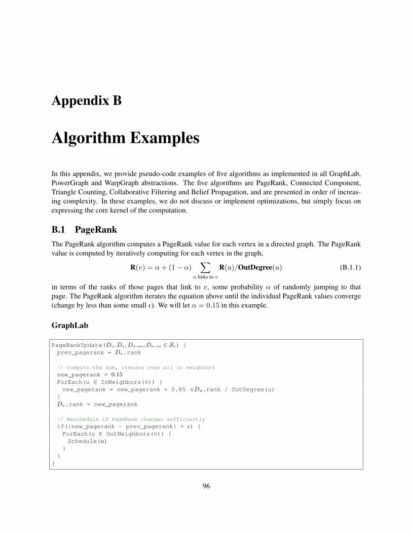
Appendix B
Algorithm Examples
In this appendix, we provide pseudo-code examples of five algorithms as implemented in all GraphLab,PowerGraph and WarpGraph abstractions. The five algorithms are PageRank, Connected Component,Triangle Counting, Collaborative Filtering and Belief Propagation, and are presented in order of increas-ing complexity. In these examples, we do not discuss or implement optimizations, but simply focus onexpressing the core kernel of the computation.
B.1 PageRankThe PageRank algorithm computes a PageRank value for each vertex in a directed graph. The PageRankvalue is computed by iteratively computing for each vertex in the graph,
R(v) = α+ (1− α)∑
u links to v
R(u)/OutDegree(u) (B.1.1)
in terms of the ranks of those pages that link to v, some probability α of randomly jumping to thatpage. The PageRank algorithm iterates the equation above until the individual PageRank values converge(change by less than some small ε). We will let α = 0.15 in this example.
GraphLab
PageRankUpdate(Dv, D∗, D∗→v, Dv→∗ ∈ Sv) {prev_pagerank = Dv.rank
// compute the sum, iterate over all in neighbors
new_pagerank = 0.15ForEach(u ∈ InNeighbors(v)) {new_pagerank = new_pagerank + 0.85 ×Du.rank / OutDegree(u)
}Dv.rank = new_pagerank
// Reschedule if PageRank changes sufficiently
if(|new_pagerank - prev_pagerank| > ε) {ForEach(u ∈ OutNeighbors(v)) {Schedule(u)
}}
}
96
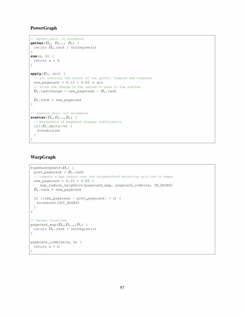
PowerGraph
// gather_nbrs: in neighbors
gather(Du, Du−v, Dv) {return Du.rank / OutDegree(u)
}sum(a, b) {return a + b
}
apply(Dv, acc) {// acc contains the result of the gather. Compute new PageRank
new_pagerank = 0.15 + 0.85 × acc// store the change in the vertex to pass to the scatter
Dv.lastchange = new_pagerank - Dv.rank
Dv.rank = new_pagerank}
// scatter_nbrs: out neighbors
scatter(Du,Du−v,Dv) {// Reschedule if PageRank changes sufficiently
if(|Dv.delta|>ε) {Schedule(u)
}}
WarpGraph
PageRankUpdate(Dv) {prev_pagerank = Dv.rank// compute a map reduce over the neighborhood selecting only the in edges
new_pagerank = 0.15 + 0.85 *map_reduce_neighbors(pagerank_map, pagerank_combine, IN_EDGES)
Dv.rank = new_pagerank
if (|new_pagerank - prev_pagerank| > ε) {broadcast(OUT_EDGES)
}}
// helper functions
pagerank_map(Du,Du−v,Dv) {return Du.rank / OutDegree(u)
}
pagerank_combine(a, b) {return a + b
}
97
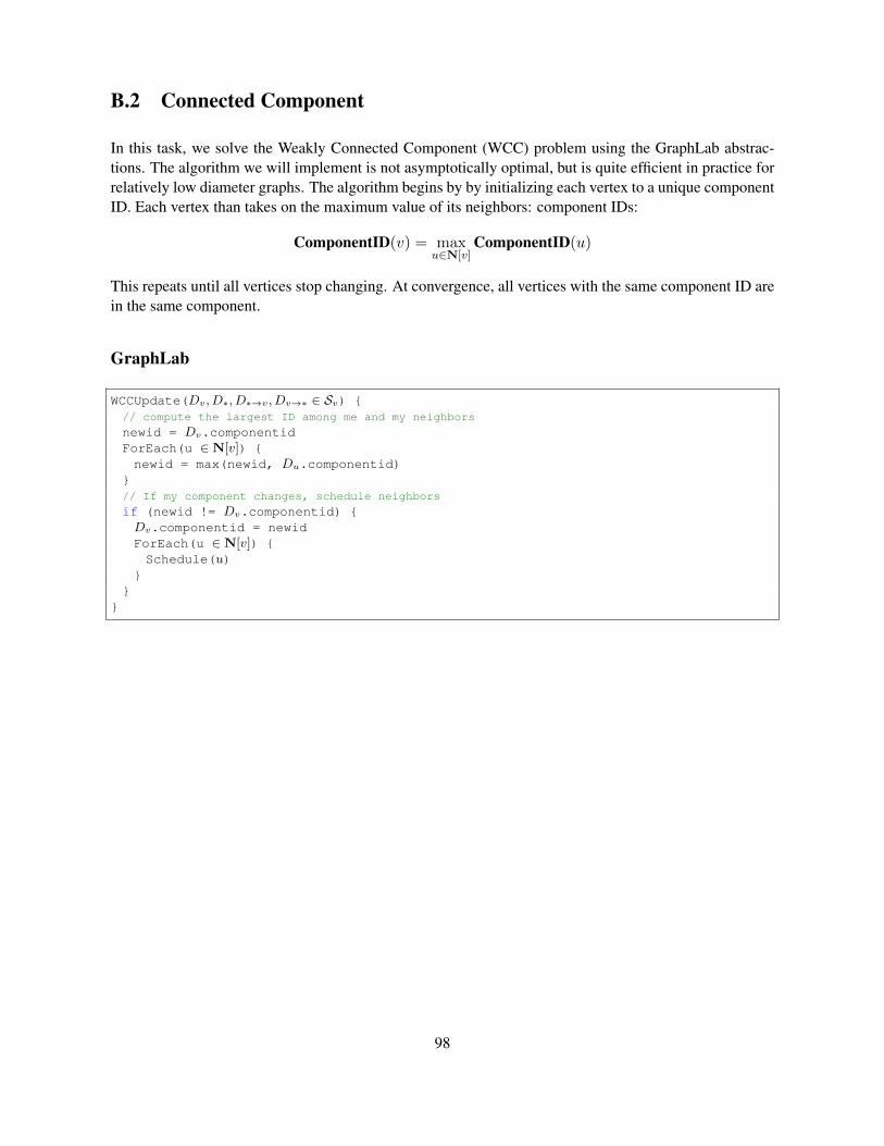
B.2 Connected Component
In this task, we solve the Weakly Connected Component (WCC) problem using the GraphLab abstrac-tions. The algorithm we will implement is not asymptotically optimal, but is quite efficient in practice forrelatively low diameter graphs. The algorithm begins by by initializing each vertex to a unique componentID. Each vertex than takes on the maximum value of its neighbors: component IDs:
ComponentID(v) = maxu∈N[v]
ComponentID(u)
This repeats until all vertices stop changing. At convergence, all vertices with the same component ID arein the same component.
GraphLab
WCCUpdate(Dv, D∗, D∗→v, Dv→∗ ∈ Sv) {// compute the largest ID among me and my neighbors
newid = Dv.componentidForEach(u ∈ N[v]) {newid = max(newid, Du.componentid)
}// If my component changes, schedule neighbors
if (newid != Dv.componentid) {Dv.componentid = newidForEach(u ∈ N[v]) {Schedule(u)
}}
}
98
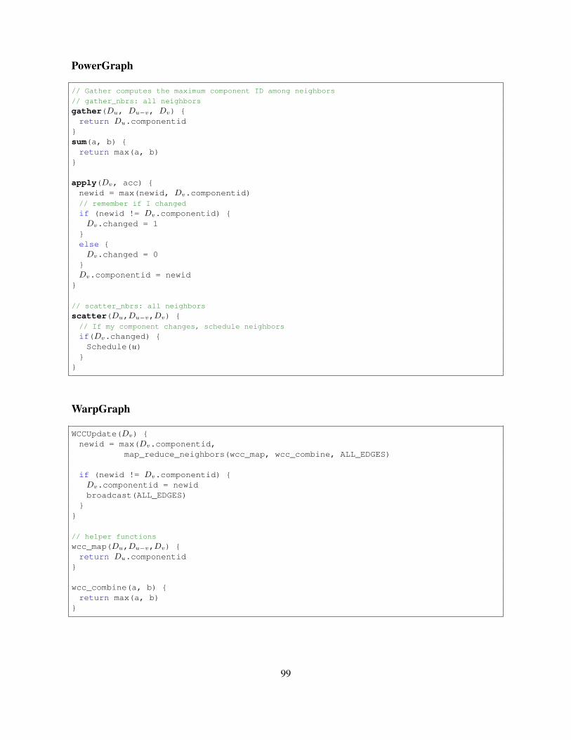
PowerGraph
// Gather computes the maximum component ID among neighbors
// gather_nbrs: all neighbors
gather(Du, Du−v, Dv) {return Du.componentid
}sum(a, b) {return max(a, b)
}
apply(Dv, acc) {newid = max(newid, Dv.componentid)// remember if I changed
if (newid != Dv.componentid) {Dv.changed = 1
}else {Dv.changed = 0
}Dv.componentid = newid
}
// scatter_nbrs: all neighbors
scatter(Du,Du−v,Dv) {// If my component changes, schedule neighbors
if(Dv.changed) {Schedule(u)
}}
WarpGraph
WCCUpdate(Dv) {newid = max(Dv.componentid,
map_reduce_neighbors(wcc_map, wcc_combine, ALL_EDGES)
if (newid != Dv.componentid) {Dv.componentid = newidbroadcast(ALL_EDGES)
}}
// helper functions
wcc_map(Du,Du−v,Dv) {return Du.componentid
}
wcc_combine(a, b) {return max(a, b)
}
99
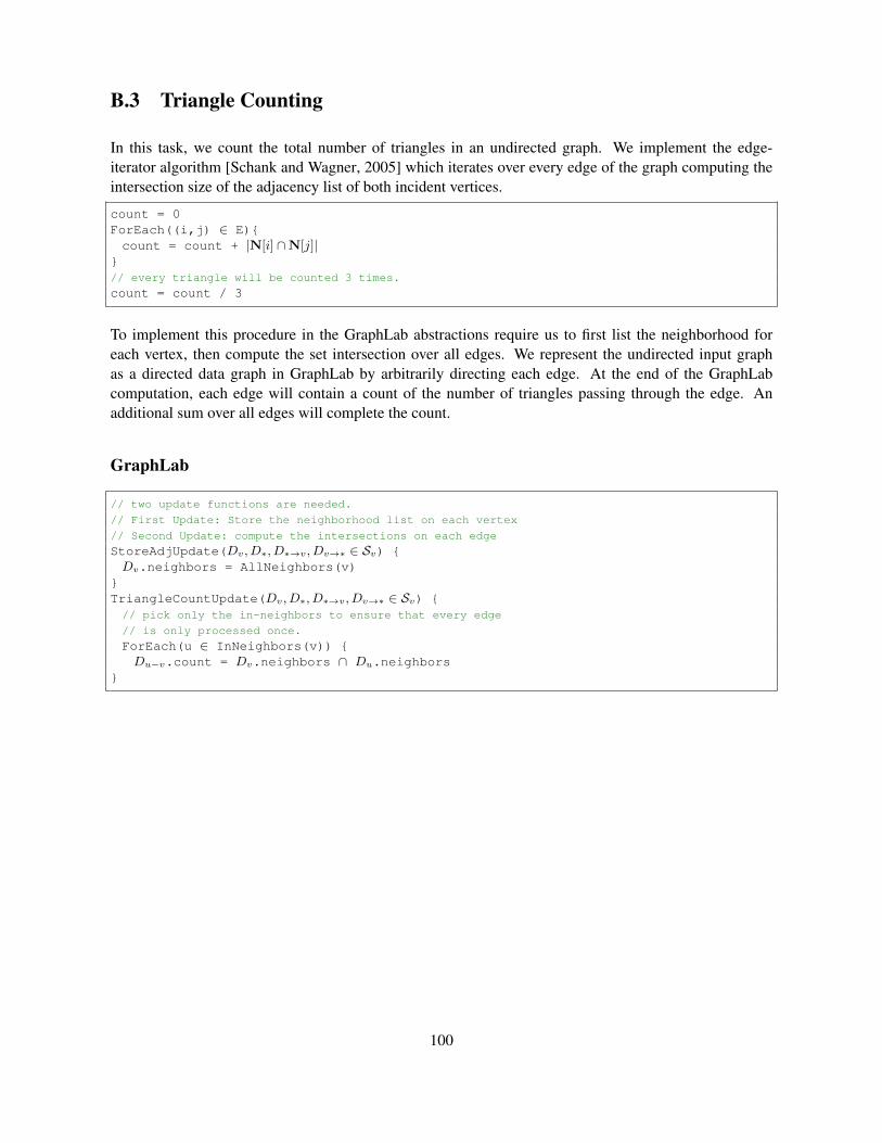
B.3 Triangle Counting
In this task, we count the total number of triangles in an undirected graph. We implement the edge-iterator algorithm [Schank and Wagner, 2005] which iterates over every edge of the graph computing theintersection size of the adjacency list of both incident vertices.
count = 0ForEach((i,j) ∈ E){count = count + |N[i] ∩N[j]|
}// every triangle will be counted 3 times.
count = count / 3
To implement this procedure in the GraphLab abstractions require us to first list the neighborhood foreach vertex, then compute the set intersection over all edges. We represent the undirected input graphas a directed data graph in GraphLab by arbitrarily directing each edge. At the end of the GraphLabcomputation, each edge will contain a count of the number of triangles passing through the edge. Anadditional sum over all edges will complete the count.
GraphLab
// two update functions are needed.
// First Update: Store the neighborhood list on each vertex
// Second Update: compute the intersections on each edge
StoreAdjUpdate(Dv, D∗, D∗→v, Dv→∗ ∈ Sv) {Dv.neighbors = AllNeighbors(v)
}TriangleCountUpdate(Dv, D∗, D∗→v, Dv→∗ ∈ Sv) {// pick only the in-neighbors to ensure that every edge
// is only processed once.
ForEach(u ∈ InNeighbors(v)) {Du−v.count = Dv.neighbors ∩ Du.neighbors
}
100
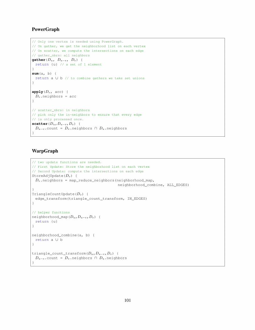
PowerGraph
// Only one vertex is needed using PowerGraph.
// On gather, we get the neighborhood list on each vertex
// On scatter, we compute the intersections on each edge
// gather_nbrs: all neighbors
gather(Du, Du−v, Dv) {return {u} // a set of 1 element
}sum(a, b) {return a ∪ b // to combine gathers we take set unions
}
apply(Dv, acc) {Dv.neighbors = acc
}
// scatter_nbrs: in neighbors
// pick only the in-neighbors to ensure that every edge
// is only processed once.
scatter(Du,Du−v,Dv) {Du−v.count = Dv.neighbors ∩ Du.neighbors
}
WarpGraph
// two update functions are needed.
// First Update: Store the neighborhood list on each vertex
// Second Update: compute the intersections on each edge
StoreAdjUpdate(Dv) {Dv.neighbors = map_reduce_neighbors(neighborhood_map,
neighborhood_combine, ALL_EDGES)}TriangleCountUpdate(Dv) {edge_transform(triangle_count_transform, IN_EDGES)
}
// helper functions
neighborhood_map(Du,Du−v,Dv) {return {u}
}
neighborhood_combine(a, b) {return a ∪ b
}
triangle_count_transform(Du,Du−v,Dv) {Du−v.count = Dv.neighbors ∩ Du.neighbors
}
101
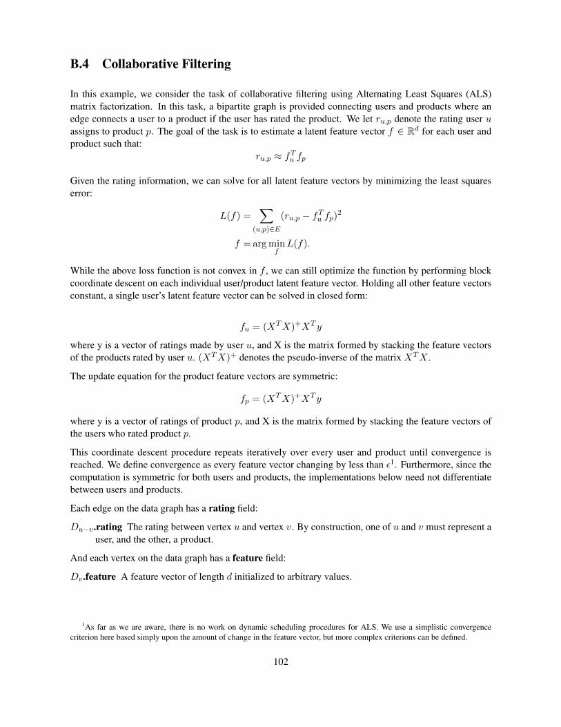
B.4 Collaborative Filtering
In this example, we consider the task of collaborative filtering using Alternating Least Squares (ALS)matrix factorization. In this task, a bipartite graph is provided connecting users and products where anedge connects a user to a product if the user has rated the product. We let ru,p denote the rating user uassigns to product p. The goal of the task is to estimate a latent feature vector f ∈ Rd for each user andproduct such that:
ru,p ≈ fTu fp
Given the rating information, we can solve for all latent feature vectors by minimizing the least squareserror:
L(f) =∑
(u,p)∈E
(ru,p − fTu fp)2
f = arg minfL(f).
While the above loss function is not convex in f , we can still optimize the function by performing blockcoordinate descent on each individual user/product latent feature vector. Holding all other feature vectorsconstant, a single user’s latent feature vector can be solved in closed form:
fu = (XTX)+XT y
where y is a vector of ratings made by user u, and X is the matrix formed by stacking the feature vectorsof the products rated by user u. (XTX)+ denotes the pseudo-inverse of the matrix XTX .
The update equation for the product feature vectors are symmetric:
fp = (XTX)+XT y
where y is a vector of ratings of product p, and X is the matrix formed by stacking the feature vectors ofthe users who rated product p.
This coordinate descent procedure repeats iteratively over every user and product until convergence isreached. We define convergence as every feature vector changing by less than ε1. Furthermore, since thecomputation is symmetric for both users and products, the implementations below need not differentiatebetween users and products.
Each edge on the data graph has a rating field:
Du−v.rating The rating between vertex u and vertex v. By construction, one of u and v must represent auser, and the other, a product.
And each vertex on the data graph has a feature field:
Dv.feature A feature vector of length d initialized to arbitrary values.
1As far as we are aware, there is no work on dynamic scheduling procedures for ALS. We use a simplistic convergencecriterion here based simply upon the amount of change in the feature vector, but more complex criterions can be defined.
102

GraphLab
ALSUpdate(Dv, D∗, D∗→v, Dv→∗ ∈ Sv) {// loop through neighbors, computing XTX and Xy
XTX = zero matrix of size d × dXy = zero vector of size d × 1
// iterate over all neighbors computing XTX and Xy
ForEach(u ∈ N[v]) {// Where ⊗ denotes the outer product
XTX = XTX + Du.feature ⊗ Du.featureXy = Xy + Du.feature × Du−v.rating
}// solve the linear system (XTX) f = (Xy) returning f
new_feature = solve(XTX, Xy)change_in_feature = |Dv.feature - new_feature|1Dv.feature = new_feature
// Schedule Neighbors if my value changes by a large amount
if (change_in_feature > ε) {ForEach(u ∈ N[v]) {Schedule(u)
}}
}
103
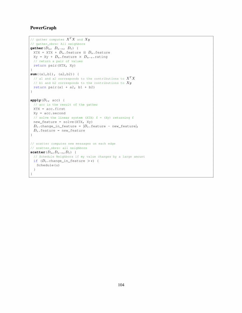
PowerGraph
// gather computes XTX and Xy// gather_nbrs: All neighbors
gather(Du, Du−v, Dv) {XTX = XTX + Du.feature ⊗ Du.featureXy = Xy + Du.feature × Du−v.rating// return a pair of values
return pair(XTX, Xy)}sum((a1,b1), (a2,b2)) {// a1 and a2 corresponds to the contributions to XTX// b1 and b2 corresponds to the contributions to Xyreturn pair(a1 + a2, b1 + b2)
}
apply(Dv, acc) {// acc is the result of the gather
XTX = acc.firstXy = acc.second// solve the linear system (XTX) f = (Xy) returning f
new_feature = solve(XTX, Xy)Dv.change_in_feature = |Dv.feature - new_feature|1Dv.feature = new_feature
}
// scatter computes new messages on each edge
// scatter_nbrs: all neighbors
scatter(Du,Du−v,Dv) {// Schedule Neighbors if my value changes by a large amount
if (Dv.change_in_feature > ε) {Schedule(u)
}}
104
WarpGraph
ALSUpdate(Dv) {(XTX, Xy) = map_reduce_neighbors(als_map, als_combine, ALL_EDGES)
// solve the linear system (XTX) f = (Xy) returning f
new_feature = solve(XTX, Xy)
change_in_feature = |Dv.feature - new_feature|1Dv.feature = new_feature
if (change_in_feature > ε) {broadcast(ALL_EDGES)
}}
// helper functions
als_map(Du,Du−v,Dv) {XTX = XTX + Du.feature ⊗ Du.featureXy = Xy + Du.feature × Du−v.rating// return a pair of values
return pair(XTX, Xy)}
als_combine((a1,b1), (a2,b2)) {// a1 and a2 corresponds to the contributions to XTX// b1 and b2 corresponds to the contributions to Xyreturn pair(a1 + a2, b1 + b2)
}
105
B.5 Belief Propagation
The Belief Propagation algorithm [Yedidia et al., 2001] is a commonly used approximate graphical modelinference procedure. While the technique can be applied to more general models, we consider the simpli-fied case of discrete pairwise Markov Random Fields (MRF) in this example.
Given a discrete probability distribution of the form
P (x1, x2 . . . , xn) ∝∏v∈V
φv(xv)∏
(u,v)∈E
φu,v(xu, xv),
The belief propagation algorithm recursively defines a message mu,v(xv) in each edge direction as wellas a belief on each vertex bv(xv).
bv(xv) ∝φv(xv)∏
u∈N[v]
mu,v(xv)
mu,v(xv) ∝∑xu
bv(xv) ∗ φu,v(xu, xv)/mv,u(xu).
The above equations are then iteratively recomputed until all beliefs converge (norm change by less thanε). At convergence, the belief on each vertex is the estimated marginal distribution of the variable.
Since the Markov Random Field is undirected, we represent this in the directed data graph by arbitrarilydirecting each edge. Each edge (u, v) therefore contains two messages, mu,v and mv,u, one in each edgedirection.
Each edge on the data graph therefore has the following fields:
Du−v.potential The potential φu,v on the edge
Du−v.message(v) The message mu,v going towards v
Du−v.message(u) The message mv,u going towards u
And each vertex on the data graph has the following fields:
Dv.potential The potential φv on the vertex
Dv.belief The estimated belief of the vertex bv
106
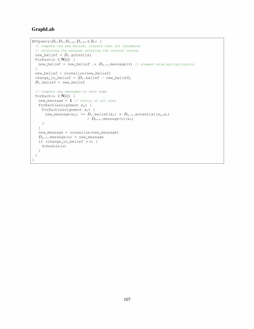
GraphLab
BPUpdate(Dv, D∗, D∗→v, Dv→∗ ∈ Sv) {// compute the new belief, iterate over all neighbors
// selecting the message entering the current vertex
new_belief = Dv.potentialForEach(u ∈ N[v]) {new_belief = new_belief .* Du−v.message(v) // element-wise multiplication
}new_belief = normalize(new_belief)change_in_belief = |Dv.belief - new_belief|1Dv.belief = new_belief
// compute new messages on each edge
ForEach(u ∈ N[v]) {new_message = 1 // vector of all ones
ForEach(assignment xu) {ForEach(assignment xv) {new_message(xu) += Dv.belief(xv) × Du−v.potential(xu, xv)
/ Du−v.message(v)(xv)}
}new_message = normalize(new_message)Du−v.message(u) = new_messageif (change_in_belief > ε) {Schedule(u)
}}
}
107
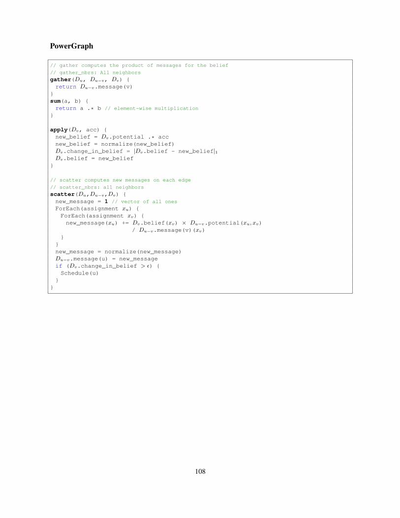
PowerGraph
// gather computes the product of messages for the belief
// gather_nbrs: All neighbors
gather(Du, Du−v, Dv) {return Du−v.message(v)
}sum(a, b) {return a .* b // element-wise multiplication
}
apply(Dv, acc) {new_belief = Dv.potential .* accnew_belief = normalize(new_belief)Dv.change_in_belief = |Dv.belief - new_belief|1Dv.belief = new_belief
}
// scatter computes new messages on each edge
// scatter_nbrs: all neighbors
scatter(Du,Du−v,Dv) {new_message = 1 // vector of all ones
ForEach(assignment xu) {ForEach(assignment xv) {new_message(xu) += Dv.belief(xv) × Du−v.potential(xu, xv)
/ Du−v.message(v)(xv)}
}new_message = normalize(new_message)Du−v.message(u) = new_messageif (Dv.change_in_belief > ε) {Schedule(u)
}}
108
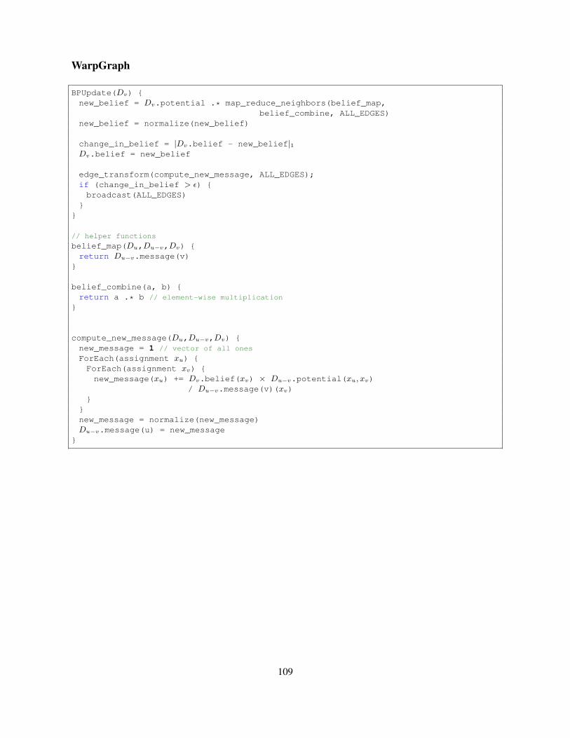
WarpGraph
BPUpdate(Dv) {new_belief = Dv.potential .* map_reduce_neighbors(belief_map,
belief_combine, ALL_EDGES)new_belief = normalize(new_belief)
change_in_belief = |Dv.belief - new_belief|1Dv.belief = new_belief
edge_transform(compute_new_message, ALL_EDGES);if (change_in_belief > ε) {broadcast(ALL_EDGES)
}}
// helper functions
belief_map(Du,Du−v,Dv) {return Du−v.message(v)
}
belief_combine(a, b) {return a .* b // element-wise multiplication
}
compute_new_message(Du,Du−v,Dv) {new_message = 1 // vector of all ones
ForEach(assignment xu) {ForEach(assignment xv) {new_message(xu) += Dv.belief(xv) × Du−v.potential(xu, xv)
/ Du−v.message(v)(xv)}
}new_message = normalize(new_message)Du−v.message(u) = new_message
}
109
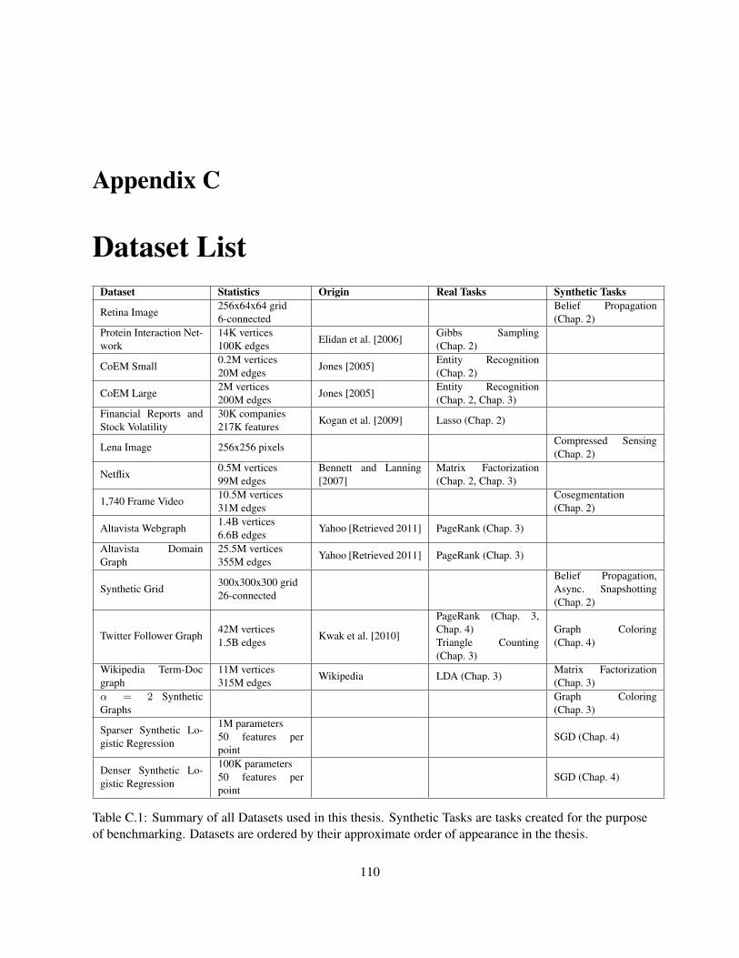
Appendix C
Dataset ListDataset Statistics Origin Real Tasks Synthetic Tasks
Retina Image256x64x64 grid6-connected
Belief Propagation(Chap. 2)
Protein Interaction Net-work
14K vertices100K edges
Elidan et al. [2006]Gibbs Sampling(Chap. 2)
CoEM Small0.2M vertices20M edges
Jones [2005]Entity Recognition(Chap. 2)
CoEM Large2M vertices200M edges
Jones [2005]Entity Recognition(Chap. 2, Chap. 3)
Financial Reports andStock Volatility
30K companies217K features
Kogan et al. [2009] Lasso (Chap. 2)
Lena Image 256x256 pixelsCompressed Sensing(Chap. 2)
Netflix0.5M vertices99M edges
Bennett and Lanning[2007]
Matrix Factorization(Chap. 2, Chap. 3)
1,740 Frame Video10.5M vertices31M edges
Cosegmentation(Chap. 2)
Altavista Webgraph1.4B vertices6.6B edges
Yahoo [Retrieved 2011] PageRank (Chap. 3)
Altavista DomainGraph
25.5M vertices355M edges
Yahoo [Retrieved 2011] PageRank (Chap. 3)
Synthetic Grid300x300x300 grid26-connected
Belief Propagation,Async. Snapshotting(Chap. 2)
Twitter Follower Graph42M vertices1.5B edges
Kwak et al. [2010]
PageRank (Chap. 3,Chap. 4)Triangle Counting(Chap. 3)
Graph Coloring(Chap. 4)
Wikipedia Term-Docgraph
11M vertices315M edges
Wikipedia LDA (Chap. 3)Matrix Factorization(Chap. 3)
α = 2 SyntheticGraphs
Graph Coloring(Chap. 3)
Sparser Synthetic Lo-gistic Regression
1M parameters50 features perpoint
SGD (Chap. 4)
Denser Synthetic Lo-gistic Regression
100K parameters50 features perpoint
SGD (Chap. 4)
Table C.1: Summary of all Datasets used in this thesis. Synthetic Tasks are tasks created for the purposeof benchmarking. Datasets are ordered by their approximate order of appearance in the thesis.
110
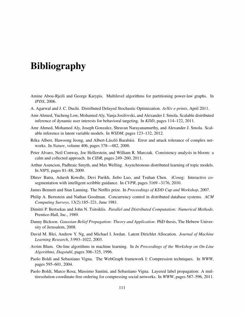
Bibliography
Amine Abou-Rjeili and George Karypis. Multilevel algorithms for partitioning power-law graphs. InIPDS, 2006.
A. Agarwal and J. C. Duchi. Distributed Delayed Stochastic Optimization. ArXiv e-prints, April 2011.
Amr Ahmed, Yucheng Low, Mohamed Aly, Vanja Josifovski, and Alexander J. Smola. Scalable distributedinference of dynamic user interests for behavioral targeting. In KDD, pages 114–122, 2011.
Amr Ahmed, Mohamed Aly, Joseph Gonzalez, Shravan Narayanamurthy, and Alexander J. Smola. Scal-able inference in latent variable models. In WSDM, pages 123–132, 2012.
Reka Albert, Hawoong Jeong, and Albert-Laszlo Barabasi. Error and attack tolerance of complex net-works. In Nature, volume 406, pages 378—482, 2000.
Peter Alvaro, Neil Conway, Joe Hellerstein, and William R. Marczak. Consistency analysis in bloom: acalm and collected approach. In CIDR, pages 249–260, 2011.
Arthur Asuncion, Padhraic Smyth, and Max Welling. Asynchronous distributed learning of topic models.In NIPS, pages 81–88, 2009.
Dhruv Batra, Adarsh Kowdle, Devi Parikh, Jiebo Luo, and Tsuhan Chen. iCoseg: Interactive co-segmentation with intelligent scribble guidance. In CVPR, pages 3169 –3176, 2010.
James Bennett and Stan Lanning. The Netflix prize. In Proceedings of KDD Cup and Workshop, 2007.
Philip A. Bernstein and Nathan Goodman. Concurrency control in distributed database systems. ACMComputing Surveys, 13(2):185–221, June 1981.
Dimitri P. Bertsekas and John N. Tsitsiklis. Parallel and Distributed Computation: Numerical Methods.Prentice-Hall, Inc., 1989.
Danny Bickson. Gaussian Belief Propagation: Theory and Application. PhD thesis, The Hebrew Univer-sity of Jerusalem, 2008.
David M. Blei, Andrew Y. Ng, and Michael I. Jordan. Latent Dirichlet Allocation. Journal of MachineLearning Research, 3:993–1022, 2003.
Avrim Blum. On-line algorithms in machine learning. In In Proceedings of the Workshop on On-LineAlgorithms, Dagstuhl, pages 306–325, 1996.
Paolo Boldi and Sebastiano Vigna. The WebGraph framework I: Compression techniques. In WWW,pages 595–601, 2004.
Paolo Boldi, Marco Rosa, Massimo Santini, and Sebastiano Vigna. Layered label propagation: A mul-tiresolution coordinate-free ordering for compressing social networks. In WWW, pages 587–596, 2011.
111
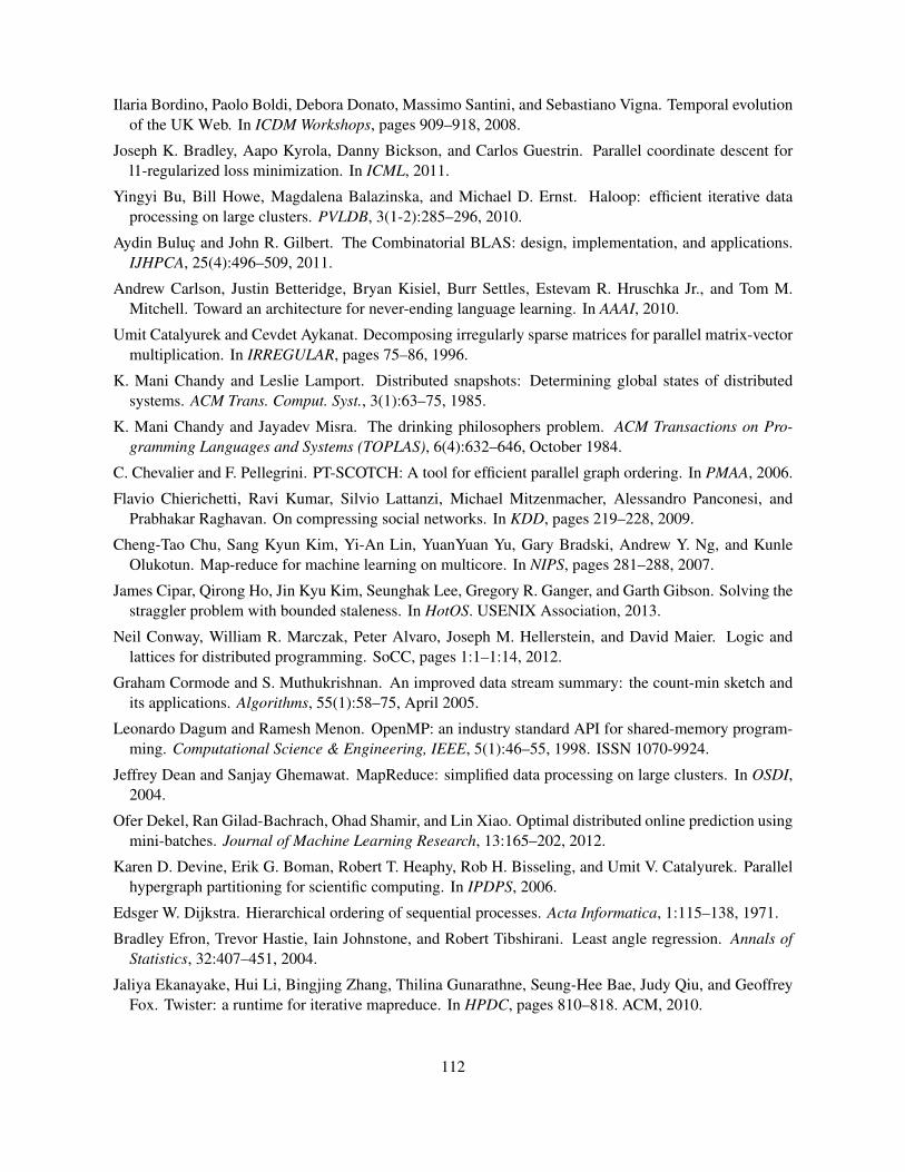
Ilaria Bordino, Paolo Boldi, Debora Donato, Massimo Santini, and Sebastiano Vigna. Temporal evolutionof the UK Web. In ICDM Workshops, pages 909–918, 2008.
Joseph K. Bradley, Aapo Kyrola, Danny Bickson, and Carlos Guestrin. Parallel coordinate descent forl1-regularized loss minimization. In ICML, 2011.
Yingyi Bu, Bill Howe, Magdalena Balazinska, and Michael D. Ernst. Haloop: efficient iterative dataprocessing on large clusters. PVLDB, 3(1-2):285–296, 2010.
Aydin Buluc and John R. Gilbert. The Combinatorial BLAS: design, implementation, and applications.IJHPCA, 25(4):496–509, 2011.
Andrew Carlson, Justin Betteridge, Bryan Kisiel, Burr Settles, Estevam R. Hruschka Jr., and Tom M.Mitchell. Toward an architecture for never-ending language learning. In AAAI, 2010.
Umit Catalyurek and Cevdet Aykanat. Decomposing irregularly sparse matrices for parallel matrix-vectormultiplication. In IRREGULAR, pages 75–86, 1996.
K. Mani Chandy and Leslie Lamport. Distributed snapshots: Determining global states of distributedsystems. ACM Trans. Comput. Syst., 3(1):63–75, 1985.
K. Mani Chandy and Jayadev Misra. The drinking philosophers problem. ACM Transactions on Pro-gramming Languages and Systems (TOPLAS), 6(4):632–646, October 1984.
C. Chevalier and F. Pellegrini. PT-SCOTCH: A tool for efficient parallel graph ordering. In PMAA, 2006.
Flavio Chierichetti, Ravi Kumar, Silvio Lattanzi, Michael Mitzenmacher, Alessandro Panconesi, andPrabhakar Raghavan. On compressing social networks. In KDD, pages 219–228, 2009.
Cheng-Tao Chu, Sang Kyun Kim, Yi-An Lin, YuanYuan Yu, Gary Bradski, Andrew Y. Ng, and KunleOlukotun. Map-reduce for machine learning on multicore. In NIPS, pages 281–288, 2007.
James Cipar, Qirong Ho, Jin Kyu Kim, Seunghak Lee, Gregory R. Ganger, and Garth Gibson. Solving thestraggler problem with bounded staleness. In HotOS. USENIX Association, 2013.
Neil Conway, William R. Marczak, Peter Alvaro, Joseph M. Hellerstein, and David Maier. Logic andlattices for distributed programming. SoCC, pages 1:1–1:14, 2012.
Graham Cormode and S. Muthukrishnan. An improved data stream summary: the count-min sketch andits applications. Algorithms, 55(1):58–75, April 2005.
Leonardo Dagum and Ramesh Menon. OpenMP: an industry standard API for shared-memory program-ming. Computational Science & Engineering, IEEE, 5(1):46–55, 1998. ISSN 1070-9924.
Jeffrey Dean and Sanjay Ghemawat. MapReduce: simplified data processing on large clusters. In OSDI,2004.
Ofer Dekel, Ran Gilad-Bachrach, Ohad Shamir, and Lin Xiao. Optimal distributed online prediction usingmini-batches. Journal of Machine Learning Research, 13:165–202, 2012.
Karen D. Devine, Erik G. Boman, Robert T. Heaphy, Rob H. Bisseling, and Umit V. Catalyurek. Parallelhypergraph partitioning for scientific computing. In IPDPS, 2006.
Edsger W. Dijkstra. Hierarchical ordering of sequential processes. Acta Informatica, 1:115–138, 1971.
Bradley Efron, Trevor Hastie, Iain Johnstone, and Robert Tibshirani. Least angle regression. Annals ofStatistics, 32:407–451, 2004.
Jaliya Ekanayake, Hui Li, Bingjing Zhang, Thilina Gunarathne, Seung-Hee Bae, Judy Qiu, and GeoffreyFox. Twister: a runtime for iterative mapreduce. In HPDC, pages 810–818. ACM, 2010.
112
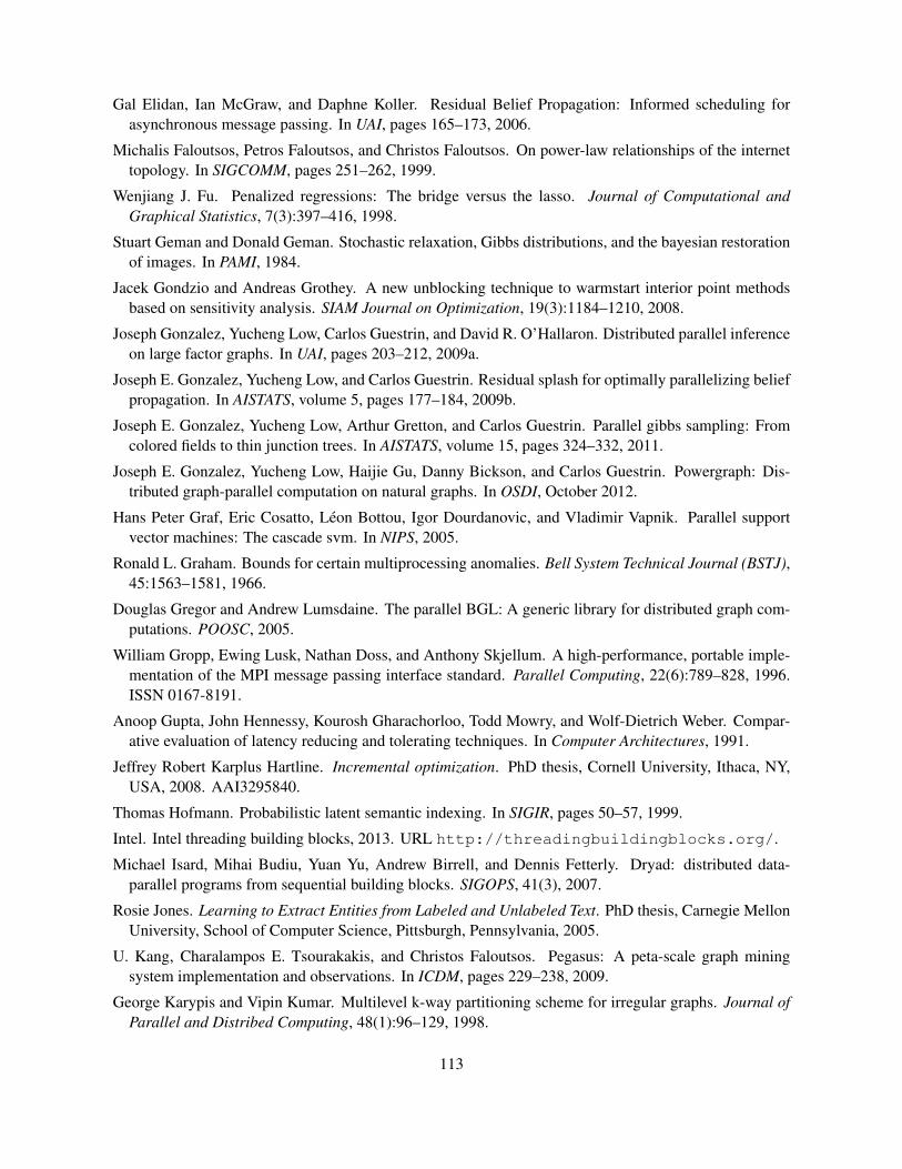
Gal Elidan, Ian McGraw, and Daphne Koller. Residual Belief Propagation: Informed scheduling forasynchronous message passing. In UAI, pages 165–173, 2006.
Michalis Faloutsos, Petros Faloutsos, and Christos Faloutsos. On power-law relationships of the internettopology. In SIGCOMM, pages 251–262, 1999.
Wenjiang J. Fu. Penalized regressions: The bridge versus the lasso. Journal of Computational andGraphical Statistics, 7(3):397–416, 1998.
Stuart Geman and Donald Geman. Stochastic relaxation, Gibbs distributions, and the bayesian restorationof images. In PAMI, 1984.
Jacek Gondzio and Andreas Grothey. A new unblocking technique to warmstart interior point methodsbased on sensitivity analysis. SIAM Journal on Optimization, 19(3):1184–1210, 2008.
Joseph Gonzalez, Yucheng Low, Carlos Guestrin, and David R. O’Hallaron. Distributed parallel inferenceon large factor graphs. In UAI, pages 203–212, 2009a.
Joseph E. Gonzalez, Yucheng Low, and Carlos Guestrin. Residual splash for optimally parallelizing beliefpropagation. In AISTATS, volume 5, pages 177–184, 2009b.
Joseph E. Gonzalez, Yucheng Low, Arthur Gretton, and Carlos Guestrin. Parallel gibbs sampling: Fromcolored fields to thin junction trees. In AISTATS, volume 15, pages 324–332, 2011.
Joseph E. Gonzalez, Yucheng Low, Haijie Gu, Danny Bickson, and Carlos Guestrin. Powergraph: Dis-tributed graph-parallel computation on natural graphs. In OSDI, October 2012.
Hans Peter Graf, Eric Cosatto, Leon Bottou, Igor Dourdanovic, and Vladimir Vapnik. Parallel supportvector machines: The cascade svm. In NIPS, 2005.
Ronald L. Graham. Bounds for certain multiprocessing anomalies. Bell System Technical Journal (BSTJ),45:1563–1581, 1966.
Douglas Gregor and Andrew Lumsdaine. The parallel BGL: A generic library for distributed graph com-putations. POOSC, 2005.
William Gropp, Ewing Lusk, Nathan Doss, and Anthony Skjellum. A high-performance, portable imple-mentation of the MPI message passing interface standard. Parallel Computing, 22(6):789–828, 1996.ISSN 0167-8191.
Anoop Gupta, John Hennessy, Kourosh Gharachorloo, Todd Mowry, and Wolf-Dietrich Weber. Compar-ative evaluation of latency reducing and tolerating techniques. In Computer Architectures, 1991.
Jeffrey Robert Karplus Hartline. Incremental optimization. PhD thesis, Cornell University, Ithaca, NY,USA, 2008. AAI3295840.
Thomas Hofmann. Probabilistic latent semantic indexing. In SIGIR, pages 50–57, 1999.
Intel. Intel threading building blocks, 2013. URL http://threadingbuildingblocks.org/.
Michael Isard, Mihai Budiu, Yuan Yu, Andrew Birrell, and Dennis Fetterly. Dryad: distributed data-parallel programs from sequential building blocks. SIGOPS, 41(3), 2007.
Rosie Jones. Learning to Extract Entities from Labeled and Unlabeled Text. PhD thesis, Carnegie MellonUniversity, School of Computer Science, Pittsburgh, Pennsylvania, 2005.
U. Kang, Charalampos E. Tsourakakis, and Christos Faloutsos. Pegasus: A peta-scale graph miningsystem implementation and observations. In ICDM, pages 229–238, 2009.
George Karypis and Vipin Kumar. Multilevel k-way partitioning scheme for irregular graphs. Journal ofParallel and Distribed Computing, 48(1):96–129, 1998.
113
Seung-Jean Kim, Kwangmoo Koh, Michael Lustig, Stephen Boyd, and Dimitry Gorinevsky. An interior-point method for large-scale l1-regularized least squares. Selected Topics in Signal Processing, IEEEJournal of, 1(4):606–617, 2007.
Shimon Kogan, Dimitry Levin, Bryan R. Routledge, Jacob S. Sagi, and Noah A. Smith. Predicting riskfrom financial reports with regression. In NAACL, pages 272–280, 2009.
Daphne Koller and Nir Friedman. Probabilistic Graphical Models: Principles and Techniques. MITPress, 2009.
Yehuda Koren. Factorization meets the neighborhood: a multifaceted collaborative filtering model. InKDD, pages 426–434, 2008.
Yehuda Koren, Robert Bell, and Chris Volinsky. Matrix factorization techniques for recommender sys-tems. Computer, 42(8):30–37, August 2009.
Oliver Kowalke. Boost context, 2013. URL http://www.boost.org/doc/libs/1_53_0/libs/context/doc/html/index.html.
Haewoon Kwak, Changhyun Lee, Hosung Park, and Sue Moon. What is twitter, a social network or anews media? In WWW, pages 591–600, 2010.
Aapo Kyrola, Guy E. Blelloch, and Carlos Guestrin. GraphChi: Large-scale graph computation on just aPC. In OSDI, October 2012.
Kevin Lang. Finding good nearly balanced cuts in power law graphs. Technical Report YRL-2004-036,Yahoo! Research Labs, Nov. 2004.
Jure Leskovec, Kevin J. Lang, Anirban Dasgupta, and Michael W. Mahoney. Community structure in largenetworks: Natural cluster sizes and the absence of large well-defined clusters. Internet Mathematics, 6(1):29–123, 2008a.
Jure Leskovec, Kevin J. Lang, Anirban Dasgupta, and Michael W. Mahoney. Statistical properties ofcommunity structure in large social and information networks. In WWW, pages 695–704, 2008b.
David D. Lewis, Yiming Yang, Tony G. Rose, and Fan Li. Rcv1: A new benchmark collection for textcategorization research. Journal of Machine Learning Research, 5:361–397, 2004.
Yucheng Low, Joseph E. Gonzalez, Aapo Kyrola, Danny Bickson, Carlos Guestrin, and Joseph M. Heller-stein. Graphlab: A new parallel framework for machine learning. In UAI, July 2010.
Yucheng Low, Deepak Agarwal, and Alexander J. Smola. Multiple domain user personalization. In KDD,pages 123–131, 2011.
Yucheng Low, Joseph E. Gonzalez, Aapo Kyrola, Danny Bickson, Carlos Guestrin, and J. M. Hellerstein.Distributed GraphLab: A Framework for Machine Learning and Data Mining in the Cloud. PVLDB,2012.
G. Malewicz, M. H. Austern, A. J.C Bik, J.C. Dehnert, I. Horn, N. Leiser, and G. Czajkowski. Pregel: asystem for large-scale graph processing. In SIGMOD, pages 135–146, 2010.
Frank McSherry, Derek Gordon Murray, Rebecca Isaacs, and Michael Isard. Differential dataflow. InCIDR, 2013.
Jayadev Misra. Detecting termination of distributed computations using markers. In SIGOPS, 1983.
Ramesh Nallapati, William Cohen, and John Lafferty. Parallelized variational EM for latent Dirichletallocation: An experimental evaluation of speed and scalability. In ICDMW, 2007.
Radford M. Neal and Geoffrey E. Hinton. A view of the EM algorithm that justifies incremental, sparse,
114
and other variants. Learning in graphical models, 89:355–368, 1998.
Jacob Nelson, Brandon Myers, A. H. Hunter, Preston Briggs, Luis Ceze, Carl Ebeling, Dan Grossman,Simon Kahan, and Mark Oskin. Crunching large graphs with commodity processors. In HotPar, 2011.
David Newman, Arthur Asuncion, Padhraic Smyth, and Max Welling. Distributed inference for latentdirichlet allocation. In NIPS, pages 1081–1088, 2008.
Kamal Nigam and Rayid Ghani. Analyzing the effectiveness and applicability of co-training. In CIKM,pages 86–93, 2000.
Christopher Olston, Benjamin Reed, Utkarsh Srivastava, Ravi Kumar, and Andrew Tomkins. Pig latin: anot-so-foreign language for data processing. In SIGMOD, pages 1099–1110, 2008.
Lawrence Page, Sergey Brin, Rajeev Motwani, and Terry Winograd. The pagerank citation ranking:Bringing order to the web. Technical Report 1999-66, Stanford InfoLab, November 1999.
Russell Power and Jinyang Li. Piccolo: building fast, distributed programs with partitioned tables. InOSDI, 2010.
Keith H. Randall. Cilk: Efficient Multithreaded Computing. PhD thesis, Department of Electrical Engi-neering and Computer Science, Massachusetts Institute of Technology, May 1998.
Ananth Ranganathan, Michael Kaess, and Frank Dellaert. Loopy sam. In IJCAI, pages 2191–2196, 2007.
Benjamin Recht, Christopher Re, Stephen Wright, and Feng Niu. Hogwild: A lock-free approach toparallelizing stochastic gradient descent. In NIPS, pages 693–701, 2011.
Ruslan Salakhutdinov, Andriy Mnih, and Geoffrey Hinton. Restricted boltzmann machines for collabora-tive filtering. In ICML, pages 791–798, 2007.
Thomas Schank and Dorothea Wagner. Finding, counting and listing all triangles in large graphs. Techni-cal report, Universitat Karlsruhe, Fakultat fur Informatik, 2005.
Athanassios G. Siapas. Criticality and parallelism in combinatorial optimization. PhD thesis, Mas-sachusetts Institute of Technology. Dept. of Electrical Engineering and Computer Science, Jan. 1996.
David B. Skillicorn, Jonathan M. D. Hill, and William F. McColl. Questions and answers about BSP.Scientific Programming, 6(3):249–274, 1997.
Alexander J. Smola and Shravan Narayanamurthy. An Architecture for Parallel Topic Models. In VLDB,2010.
Le Song, Arthur Gretton, Danny Bickson, Yucheng Low, and Carlos Guestrin. Kernel belief propagation.In AISTATS, volume 15, pages 707–715, 2011.
Isabelle Stanton and Gabriel Kliot. Streaming graph partitioning for large distributed graphs. TechnicalReport MSR-TR-2011-121, Microsoft Research, November 2011.
Siddharth Suri and Sergei Vassilvitskii. Counting triangles and the curse of the last reducer. In WWW,pages 607–614, 2011.
Robert Tibshirani. Regression shrinkage and selection via the lasso. Journal of the Royal StatisticalSociety (Series B), 58:267–288, 1996.
Kyle Wheeler, Richard Murphy, and Douglas Thain. Qthreads: An api for programming with millions oflightweight threads. In IPDPS, pages 1–8, 2008.
Reynold Xin, Joseph Gonzalez, and Michael Franklin. Graphx: A resilient distributed graph system onspark. In GRADES SIGMOD Workshop, 2013.
115

Yahoo. Yahoo! Altavista web graph, Retrieved 2011. URL http://webscope.sandbox.yahoo.com/.
J.S. Yedidia, W.T. Freeman, and Y. Weiss. Bethe free energy, kikuchi approximations, and belief propa-gation algorithms. Technical report, Mitsubishi Electric Research Laboratories, 2001.
E. Alper Yildirim and Stephen J. Wright. Warm-start strategies in interior-point methods for linear pro-gramming. SIAM Journal on Optimization, 12:782–810, March 2002.
Matei Zaharia, Mosharaf Chowdhury, Michael J. Franklin, Scott Shenker, and Ion Stoica. Spark: clustercomputing with working sets. In HotCloud, 2010.
Yanfeng Zhang, Qixin Gao, Lixin Gao, and Cuirong Wang. Priter: a distributed framework for prioritizediterative computations. In SOCC, 2011.
Yunhong Zhou, Dennis Wilkinson, Robert Schreiber, and Rong Pan. Large-scale parallel collaborativefiltering for the netflix prize. In AAIM, pages 337–348, 2008.
Martin Zinkevich, Markus Weimer, Alexander J. Smola, and Lihong Li. Parallelized stochastic gradientdescent. In NIPS, pages 2595–2603, 2010.
116

Carnegie Mellon University does not discriminate in admission, employment, or administration of its programs or activities on the basis of race, color, national origin, sex, handicap or disability, age, sexual orientation, gender identity, religion, creed, ancestry, belief, veteran status, or genetic information. Futhermore, Carnegie Mellon University does not discriminate and if required not to discriminate in violation of federal, state, or local laws or executive orders.
Inquiries concerning the application of and compliance with this statement should be directed to the vice president for campus affairs, Carnegie Mellon University, 5000 Forbes Avenue, Pittsburgh, PA 15213,telephone, 412-268-2056
Carnegie Mellon University5000 Forbes AvenuePittsburgh, PA 15213