Cambridge International A and AS Level Geography © Hodder Education 20111

Geographical skills

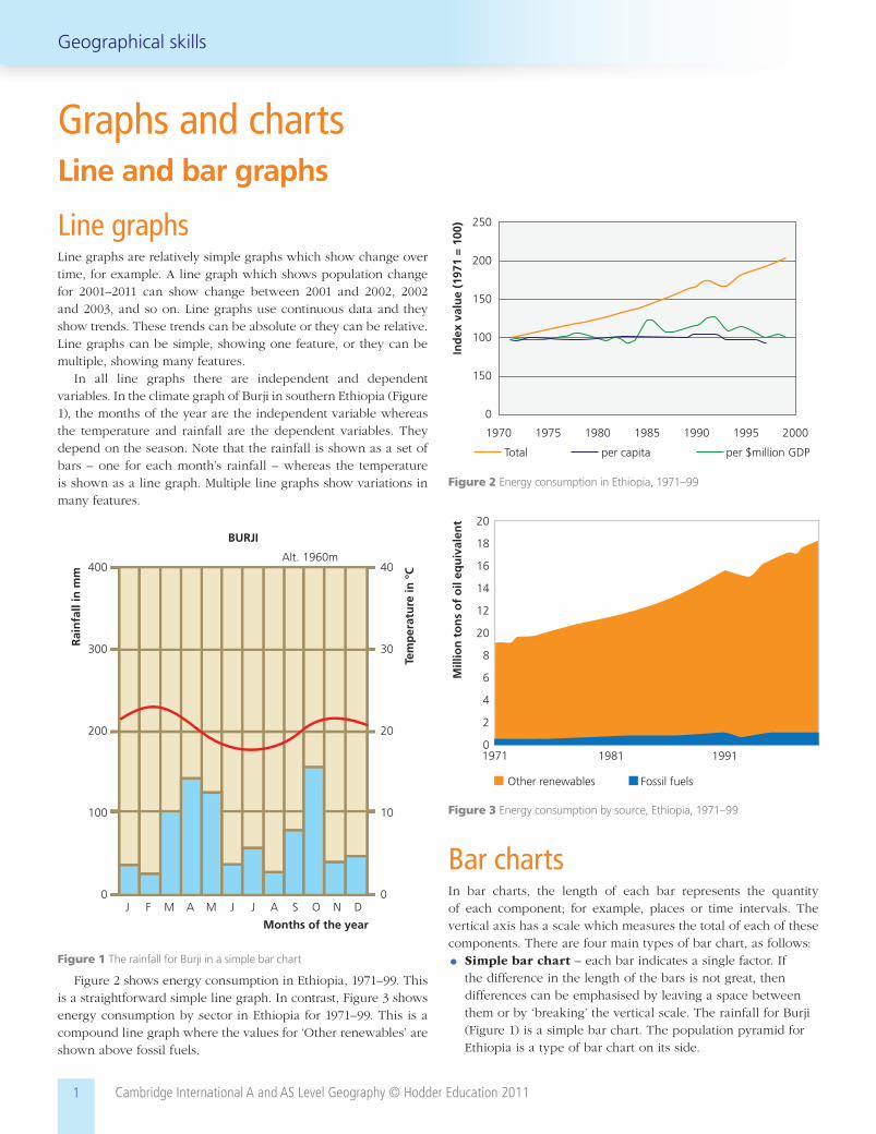
Line graphsLine graphs are relatively simple graphs which show change over time, for example. A line graph which shows population change for 2001–2011 can show change between 2001 and 2002, 2002 and 2003, and so on. Line graphs use continuous data and they show trends. These trends can be absolute or they can be relative. Line graphs can be simple, showing one feature, or they can be multiple, showing many features.

In all line graphs there are independent and dependent variables. In the climate graph of Burji in southern Ethiopia (Figure 1), the months of the year are the independent variable whereas the temperature and rainfall are the dependent variables. They depend on the season. Note that the rainfall is shown as a set of bars – one for each month’s rainfall – whereas the temperature is shown as a line graph. Multiple line graphs show variations in many features.

BURJI

Rai

nfa

ll in

mm

Tem

per

atu

re in

°C

Alt. 1960m

Months of the year

J F M A M J J A S O N D

40

30

20

10

0

400

300

200

100

0

Figure 1 The rainfall for Burji in a simple bar chart

Figure 2 shows energy consumption in Ethiopia, 1971–99. This is a straightforward simple line graph. In contrast, Figure 3 shows energy consumption by sector in Ethiopia for 1971–99. This is a compound line graph where the values for ‘Other renewables’ are shown above fossil fuels.

Total per capita per $million GDP

250

Ind

ex v

alu

e (1

971

= 1

00)

200

150

100

150

0

1970 1975 1980 1985 1990 1995 2000

Figure 2 Energy consumption in Ethiopia, 1971–99

1971

Other renewables Fossil fuels

20

Mill

ion

to

ns

of

oil

equ

ival

ent

18

16

14

12

20

8

6

4

2

01981 1991

Figure 3 Energy consumption by source, Ethiopia, 1971–99

Bar chartsIn bar charts, the length of each bar represents the quantity of each component; for example, places or time intervals. The vertical axis has a scale which measures the total of each of these components. There are four main types of bar chart, as follows:

● Simple bar chart – each bar indicates a single factor. If the difference in the length of the bars is not great, then differences can be emphasised by leaving a space between them or by ‘breaking’ the vertical scale. The rainfall for Burji (Figure 1) is a simple bar chart. The population pyramid for Ethiopia is a type of bar chart on its side.

Graphs and chartsLine and bar graphs

Cambridge International A and AS Level Geography © Hodder Education 20112

Geographical skills

● Multiple or group bar chart – features are grouped together on one graph to help comparison.

● Compound or component bar chart – various elements or factors are grouped together on one bar (the most stable element or factor is placed at the bottom to avoid disturbance).

● Percentage compound or component bar chart – a variation on the compound bar chart. It is used to compare

features by showing the percentage contribution. These graphs do not give a total in each category, but compare relative changes in percentages.

Figure 4 shows a bar chart showing AIDS cases in Ethiopia for 1986–2001 by age and sex.

Activities

1 Make a graph similar to the one for Burji, showing the climate data for Addis Ababa.

Table 1 Climate data for Addis Ababa

J F M A M J J A S O N D

Mean temp. (º C) 14 15 17 17 17 16 16 15 15 15 14 14

Rainfall (mm) 13 35 67 91 81 117 247 255 167 29 8 5

Describe the climate shown by the graph you have drawn.

2 Plot the data for sunshine hours by using a simple bar chart.

Table 2 Average sunshine per day in Addis Ababa

J F M A M J J A S O N D

Average sunshine per day (hours)

8.7 8.2 7.6 8.1 6.5 4.8 2.8 3.2 5.2 7.6 6.7 7.0

Describe and suggest reasons for the variation in sunshine hours.

3 Table 3 shows foreign investment into Korea in $US millions.

Table 3 Foreign investment into Korea in $US millions

Year Total USA Japan UK

1985 532.2 108.0 364.3 12.3

1995 1947.2 644.9 418.3 86.7

2000 15 216.7 2922.0 2448.0 84.0

2005 11 563.5 2689.8 1878.8 2307.8

a Use a compound bar graph to show how foreign investment varied between 1985, 1995 and 2005. Draw one bar for 1985, one for 1995 and one for 2005.

b Describe the changes in foreign investment as shown in your bar chart.

10 000

8000

Nu

mb

er o

f A

IDS

case

s

Age group

6000

14000

2000

Male

Female

0

0–4 5–14 15–19 20–24 25–29 30–34 35–59 06–64 65–69 70+

Figure 4 AIDS cases in Ethiopia 1986–2001 by age and sex

Cambridge International A and AS Level Geography © Hodder Education 20113

Geographical skills

Pie chartsPie charts and proportional pie charts are frequently used on maps to show variations in size and composition of a geographical feature. Every 3.6 ° on the pie chart represents 1 per cent, thus the 360 ° of the circle represents 100 per cent. To plot values, fi rst convert them to percentages and then multiply by 3.6. This gives the number of degrees that each segment will be.

Using proportional circlesThe size (area) of the circle has to be proportional to the value it represents. The area of a circle is found by using the formula ∏r2,

therefore the circles are drawn in relation to the square root of the value. Decide on the size of the largest circle to be used. Write down its radius (r). Work out the square root of all the values to be mapped. Using the square root of the largest value to be mapped, work out the value (v) that it must be multiplied by in order to make the actual circle on the map. Then multiply all the other square roots by the value (v).

The advantages of pie charts and proportional pie charts are that they are very clear, can show a large amount of data, and can be very striking (see Figure 5). The main disadvantage – especially of proportional pie charts – is that they over-emphasise large values, and so small values are not as clear (see Figure 6). They also require time, care and patience to draw.

(1985) (2000)Employment & GRDP11:4,500,000

0 50km

GangwonGyeongii

Chungbuk

Chungnam Gyeongbuk

Daegu

Jeonbuk

Seoul

Incheon

Busan

Jeonnam

Gyeongnam

Gangwon

Gyeongii

ChungbukChungnam

GyeongbukDaegu

Jeonbuk

Seoul

Incheon

BusanJeonnam

Gyeongnam

Daejeon

Gwangju

The tertiaryindustries

The primaryindustries

The secondaryindustries

Jeju Jeju

Over 250210∼250180∼210150∼180Under 150(thousand won)

GRDP per capitaOver 13001100∼1300900∼1100700∼900Under 700(thousand won)

GRDP per capita

(Annual Report on the EconomicallyActive Population Survey 2001)(Social Indicators in Korea 2001)

(Korea Statistical Yearbook 2001)(thousand persons)

(1985 Population and Housing Census Report)(Gross Regional Domestic Product 1985∼1991)

Employed persons5000300020001000500(thousand persons)

Employment by Industry2 Products by Industry3The primaryindustries

50.4%

34.0%

17.9%

10.9%

14.3%

22.5%

27.6%

20.2%

35.3%

43.5%

54.5%

68.9%

26.6%

14.7%

8.7%

6.4%

22.5%

29.7%

29.7%

32.3%

50.9%

55.6%

61.6%

61.3%

The secondaryindustries

The tertiaryindustries

The primaryindustries

The secondaryindustries

The tertiaryindustries

1970(9,617)

1980(13,683)

1990(18,085)

2000(21,061)

(hundred million won)

1970(27,713)

1980(381,484)

1990(1,795,390)

1999(3,798,121)

Figure 5 Proportional pie charts to show GDP and industrial structure in South Korea

Cambridge International A and AS Level Geography © Hodder Education 20114

Geographical skills

Industry

Transportation

Agriculture

Commercial and publicservices

Residential

Non-energy uses and‘other’ consumption

0%

0%

2%

93%

3%2%

Figure 6 Pie chart showing energy consumption by sector, Ethiopia

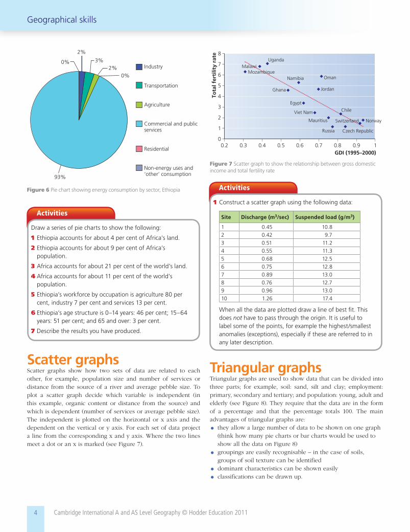
Scatter graphsScatter graphs show how two sets of data are related to each other, for example, population size and number of services or distance from the source of a river and average pebble size. To plot a scatter graph decide which variable is independent (in this example, organic content or distance from the source) and which is dependent (number of services or average pebble size). The independent is plotted on the horizontal or x axis and the dependent on the vertical or y axis. For each set of data project a line from the corresponding x and y axis. Where the two lines meet a dot or an x is marked (see Figure 7).

Activities

Draw a series of pie charts to show the following:

1 Ethiopia accounts for about 4 per cent of Africa’s land.

2 Ethiopia accounts for about 9 per cent of Africa’s population.

3 Africa accounts for about 21 per cent of the world’s land.

4 Africa accounts for about 11 per cent of the world’s population.

5 Ethiopia’s workforce by occupation is agriculture 80 per cent, industry 7 per cent and services 13 per cent.

6 Ethiopia’s age structure is 0–14 years: 46 per cent; 15–64 years: 51 per cent; and 65 and over: 3 per cent.

7 Describe the results you have produced.

8

7

6

5

4

3

2

1

0

Tota

l fer

tilit

y ra

te

GDI (1995–2000)0.2 0.3 0.4 0.5 0.6 0.7 0.8 0.9 1

UgandaMalawi

MozambiqueNamibia

Ghana Jordan

Egypt

Viet Nam

Mauritius

Russia

Chile

Switzerland

Czech Republic

Norway

Oman

Figure 7 Scatter graph to show the relationship between gross domestic income and total fertility rate

Activities

1 Construct a scatter graph using the following data:

Site Discharge (m3/sec) Suspended load (g/m3)

1 0.45 10.8

2 0.42 9.7

3 0.51 11.2

4 0.55 11.3

5 0.68 12.5

6 0.75 12.8

7 0.89 13.0

8 0.76 12.7

9 0.96 13.0

10 1.26 17.4

When all the data are plotted draw a line of best fi t. This does not have to pass through the origin. It is useful to label some of the points, for example the highest/smallest anomalies (exceptions), especially if these are referred to in any later description.

Triangular graphsTriangular graphs are used to show data that can be divided into three parts; for example, soil: sand, silt and clay; employment: primary, secondary and tertiary; and population: young, adult and elderly (see Figure 8). They require that the data are in the form of a percentage and that the percentage totals 100. The main advantages of triangular graphs are:

● they allow a large number of data to be shown on one graph (think how many pie charts or bar charts would be used to show all the data on Figure 8)

● groupings are easily recognisable – in the case of soils, groups of soil texture can be identified

● dominant characteristics can be shown easily ● classifications can be drawn up.

Cambridge International A and AS Level Geography © Hodder Education 20115

Geographical skills

FrSwJp

UKGhana

WorldBrazil

BoLDCs

MDCs

10 90

20 80

30 70

40 60

50 50

60 40

70 30

80 20

90 10

1000 10 20 30 40 50 60 70 80 90 100

0

0 100

Children(0–19)

Adults(20–59)

Elderly(60+)

KeyLDCs Less developed countriesMDCs More developed countriesUK United KingdomFr FranceSw SwedenJp JapanBo Bolivia

Figure 8 Triangular graph to show population composition

They can be tricky and it is easy to get confused, especially if care is not taken. However, they provide a fast, reliable way of classifying large amounts of data that have three components.

AcknowledgementsThe publishers would like to thank the following for permission to reproduce copyright material:

Figure 5 from the Korea Statistical Yearbook, 2000; Figure 7 from the Korea Statistical Yearbook, 2006; Figure  8 from Advanced Geography: Concepts and Cases (Hodder Education, 1999); Figure 9 from the Academy of Korean Studies.

Activities

1 On a copy of the triangular graph (Figure 9), show how the workforce of Korea has changed over time.

10 90

20 80

30 70

40 60

50 50

60 40

70 30

80 20

90 10

1000 10 20 30 40 50 60 70 80 90 100

0

0 100

perc

enta

ge e

mpl

oyed

in se

cond

ary

indu

stry

percentage employed in primary industry

percentage employed in tertiary industry

Figure 9 Triangular graph

Table 4 Changing workforce of Korea

YearPrimary industries

Secondary industries

Tertiary industries

1970 50.4 14.3 35.3

1980 34.0 22.5 43.5

1990 17.9 27.6 54.5

2000 10.9 20.2 68.9