Gravity Models: Theoretical Foundations and related estimation

issues

ARTNet Capacity Building Workshop for Trade ResearchPhnom Penh, Cambodia

2-6 June 2008

Outline

1. Theoretical foundations• From Tinbergen (1962)….• … to Anderson and Van Wincoop (2003)

• The question of zeros in the trade matrix (Helpman, Melitz and Rubinstein, 2005)

2. Empirical equations and some related estimation issues

The Gravity Model: what it is?

Econometric model (ex-post analysis)Workhorse in a number of fields. It has been used to analyze the impact of GATT/WTO membership, RTAs, currency unions, migration flows, FDI between countries, disasters ...Initially, not based on a theoretical model

What explain its popularity? • High explanatory power• Data easily available• There are established standard practices that facilitate the work of

researchers

The gravity model: the origins

Proposed by Tinbergen (1962) to explain international bilateral tradeCalled “gravity model” for its analogy with Newton’s law of universal gravitation

The gravity model: the origins

Newton’s Law of Universal Gravitation

Fij = G Mi MjDij

2

F= attractive force; M= mass; D=distance; G = gravitational constant

Gravity Model specification similar to Newton’s Law

Xij = K Yiα Yj

β

Tijθ

Xij= exports from i to j; or total trade (i.e Xij +Xji)Y= economic size (GDP, POP) T =Trade costs

Standard proxies for trade costs in gravity equations

DistanceAdjacencyCommon language Colonial linksCommon currencyIsland, LandlockedInstitutions, infrastructures, migration flows,...Surprisingly, bilateral tariff barriers often missing

The gravity model: the origins

Bilateral trade between any two countries is positively related to their size and negatively related to the trade cost between them

Which country-pair trade more?

Country B

Country A

DistanceCountry D

Country C

The gravity model: the originsEstimated gravity equation ...

Newton’s Law-based Normal Trade

ln (Xij) = = C + a ln(Yi) + b ln(Yj) +c ln(distij) + uij

Theoretical foundations for the gravity equation

Deardoff (1998) “I suspect that just about any plausible model of trade would yield something very like the gravity equation”

Theoretical foundations of gravity equation: historical evolution

Anderson (1979)• Armington assumption (i.e. goods differentiated by

country of origin)Bergstrand (1990)

• Anderson and Monopolistic competition• But, he continue using existing price indexes instead

of those derived through the theoryVan Wincoop (2003)

• Monopolistic competition• Provide a practical way to estimate gravity

coefficients in a cross sectionHelpman et al. (2006)

• Heterogenous firms model of trade

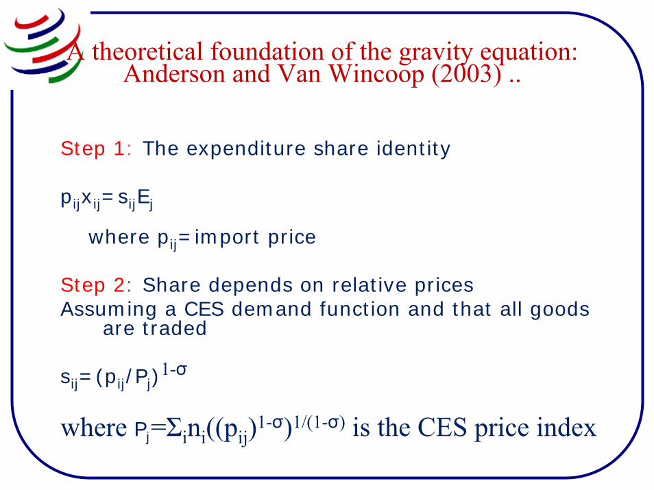
A theoretical foundation of the gravity equation: Anderson and Van Wincoop (2003) ..

Step 1: The expenditure share identity

pijxij=sijEj

where pij=import price

Step 2: Share depends on relative pricesAssuming a CES demand function and that all goods

are traded

sij=(pij/Pj)1-σ

where Pj=Σini((pij)1-σ)1/(1-σ) is the CES price index

… A theoretical foundation of the gravity equation: Anderson and Van Wincoop (2003)

Step 3:adding the pass-through equation

pij=poitij

superscript o denotes producer pricet=bilateral trade costs

Step 4: aggregating across varietiesXij=nisijEj=ni (po

itij /Pj)1-σ Ej

… A theoretical foundation of the gravity equation: Anderson and Van Wincoop (2003)

Step 5:using GE condition (summing over all markets, including country i’s own market)

Yi= ΣiXij

Solving for nipi and substituting in eq. in Step 4 yields:

A theoretical foundation of the gravity equation: Anderson and Van Wincoop

(2003)Step 6: the reduced form of a intra-industry trade model

Yi Yj tij1-σ

Xij = ΠiPj

where Πi=(Σi tij1-σ Ej/Pj

1-σ)1/(1-σ)

P and Π = Multilateral Resistance Terms

Countries’ distance from the “Rest of the World”matters for their bilateral trade

Which country-pair trade more?

Country B Country A

Rest of the World

A theoretical foundation for the gravity equation: the intuition

Country BCountry A

A theoretical foundation for the gravity equation: the intuition

The important contribution of Anderson and Van Wincoop’s paper has been to highlight that bilateral trade is determined by relativetrade costs

Estimated gravity equation ...Theoretically Founded “Normal” Trade

Normal trade with resistances

ln (Xij) = =K + a ln(Yi) + b ln(Yj) +c ln(bilateral trade barriersij) + d ln(MRTi) + e ln(MRTj) + uij

MRT= Multilateral Resistance Term

MRT are not observable.

Multilateral Trade Resistances and the gravity equation

3 ways to take MTR into account:1. Use an iterative method to solve MRT as function of

observable (see Anderson and Van Wincoop, 2003) 2. Calculate Remoteness (trade/GDP weighted average distances

from the rest of the world) whereby Remotenessi= Σ j distancejj/(GDPj/GDPW)

3. Use country fixed effects for importers and for exporters

Country-specific fixed effects

Importer (exporter) dummy= it is a 0,1 dummy that denotes the importer (exporter)They control for unobserved characteristics of a country, i.e. any country characteristic that affect its propensity to import (export) They are used to proxy each country’s remoteness They do not control for unobserved characteristics of pair of countries e.g. they have a RTA in place (need country pair fixed effects for this)

Estimated gravity equation ...using fixed effects: Cross Country Analysis

In cross country analysis MRT are fixed. Therefore, using country fixed effects yields consistent estimations

ln (Xij) = K +c ln(bilateral trade barriersij) ++Σ di Ii + Σ ei Ij + uij

Where I=country specific dummiesThere are 2n dummies. Total observations= n(n-1)

It is Impossible to estimate the coefficient for GDP and other country-specific variables

Estimated gravity equation ...using fixed effects: Panel Data (1)

It is now POSSIBLE to estimate the coefficient for GDP and other country-specific variables

ln (Xij)t =K + a ln(Yi)t + b ln(Yj)t +c ln(bilateraltrade barriersij)t +Σ di Ii + Σ ei Ij + uij

Where I=country specific dummiesThere are 2n such dummies Total observations= n(n-1)T

It is still not possible to estimate time-invariant country specific characteristics (eg. Island, landlockedness)There may be a bias due to the variation over time of MTRs

Estimated gravity equation ... using time-varying fixed effects: Panel Data (2)

In the case of a panel, MRTs may change over time (variation in transport costs or composition of trade)

ln (Xij)t = =K +c ln(bilateral trade barriersij)t +Σ dit Iit+ + Σ eit Ijt + Σ fτ Lτ +uij

Where I=time-varying country specific dummies;L=time dummy (to take global inflation trends into

account)There are 2nT+T dummies, where T denotes the

time periodImpossible to estimate the coefficient of GDP

Estimated gravity equation ... using country-pair fixed effects: Panel Data

(3)address the bias due to the correlation between the bilateral

trade barriers and the MRTs

ln (Xij)t = =K + a ln(Yi)t + b ln(Yj)t +c ln(bilateral trade barriersij)t + Σ dij Iij + uij

Where I= country-pair dummies; There are n(n-1)/2 such dummies

Disadvantage: coefficients of bilateral variables are estimated on the time dimension of the panel AND cannot estimate coefficient for distance, common border, common language …

A solution: Use random effects and the Hausman test to choose between random and fixed effect estimation

How to proceed?

Sensitivity analysis, test the robustness of the results to alternative specifications of the gravity equationsReport the results for the different equations estimated

Recent Theoretical Developments

Recently, Helpman et al. (2006) derived a gravity equation from an heterogeneous firms model of tradeThe importance of this derivation relates to three issues that previous models of trade could not explain:

• zero-trade observations• Asymmetric trade flows• The extensive margin of trade: more

countries trade over time

The incidence of zero trade

How to handle zero-trade data?

Traditionally,When taking logs, zero observations are dropped from the sample. Then, the OLS estimation is run on positive values.

Take the log(1+Xij), but then use Tobitestimation as the OLS would provide biased results

OLS Bias if zero observations are not used

OLS Fit

True fit

X

Tradeij Recent studies (Felbermayr and Kohler, 2005; Helpman, 2006) that have included unrecorded trade flows in gravity equations have tended to find thatWTO membership has a strong and significant effect on the formation of bilateral trading relationships.

How to handle zero-trade data?

More recently,Helpman et al. (2006) claim: biased results using the standard

approach In their model, differences in trade costs across countries and firms heterogeneity account for both asymmetric trade flows and zero trade. Zero trade occurs when the productivity of all firms in country i is below the threshold that would make exporting to j profitable.

Problem: the probability of having positive trade between 2 countries is correlated with unobserved characteristics of that country pair. These characteristics also affect the volume of their bilateral trade, given that they trade.

How to handle zero-trade data?

More recently,Helpman et al. (2006)provide the following solution:

Use 2 stage estimation1. Probit on the likelihood that 2 countries trade2. Then, estimate the gravity equation, introducing the

estimated Mills Ratio to control for sample selection bias (as in the estimation of a selection model a la Heckman) and a variable controlling for firms heterogeneity. Selection bias and omitted variable problem.

References

Anderson J.E. (1979) “A Theoretical Foundation for the Gravity Equation”, AER, 69(1):106-116Anderson J. and E. Van Wincoop (2003) “Gravity with Gravitas: A solution to the Border Puzzle” AER, 93:170-192Bergstarnd J.H. (1990) “The Heckscher-Ohlin-Samuelson model, the Linder Hypothesis, and the Determinants of Bilateral Intra-industry Trade” Economic Journal, 100(4):1216-1229Baldwin R. and D. Taglioni (2006) “Gravity for Dummies and Dummies for Gravity Equations”, NBER WP 12516Deardoff (1998)”Determinants of Bilateral Trade: Does Gravity Work in a Neoclassical Framework?” in J.A. Frankel (ed.) The Regionalization of the World Economy, Chicago: University of Chicago PressEvenett S. and W. Keller (2002) “On Theories Explaining the Gravity Equation”, Journal of Political Economy, 110:281-316Feenstra, R.(2004) Advanced International Trade, MIT PressHead K. (2003)”Gravity for Beginners”, mimeo, University British ColumbiaHelpman, Melitz and Rubinstain (2006) “Trading Partners and Trading Volumes” mimeo.Westerlund J. and F. Wilhelmsson (2006) “Estimating the gravity Model without Gravity Using Panel Data”, at www.nek.lu.se

Data sources

Feenstra bilateral trade data (1962-2000) from UN Comtradehttp://cid.econ.ucdavis.edu/data/undata/undata.htmlCEPII Distance and other geography variableshttp://www.cepii.fr/anglaisgraph/bdd/distances.html