gravity wave activity during stratospheric sudden warmings...

JOURNAL OF GEOPHYSICAL RESEARCH, VOL. ???, XXXX, DOI:10.1029/,

Gravity Wave Activity during Stratospheric Sudden1

Warmings in the 2007/08 Northern Hemisphere2

Winter3

L. Wang

NorthWest Research Associates Inc., Colorado Research Associates Div.,4

Boulder, Colorado, USA5

M. J. Alexander

NorthWest Research Associates Inc., Colorado Research Associates Div.,6

Boulder, Colorado, USA7

L. Wang, NorthWest Research Associates Inc., Colorado Research Associates Div., 3380

Mitchell Lane, Boulder, CO 80301, USA ([email protected])

D R A F T April 20, 2009, 5:08pm D R A F T

X - 2 WANG AND ALEXANDER: GRAVITY WAVE ACTIVITY DURING SSWS

Abstract. We use temperature retrievals from the Constellation Observ-8

ing System for Meteorology, Ionosphere and Climate (COSMIC)/Formosa9

Satellite Mission 3 (FORMOSAT-3) and Challenging Minisatellite Payload10

(CHAMP) Global Positioning Satellite (GPS) radio occultation profiles and11

independent temperature retrievals from the EOS satellite High Resolution12

Dynamics Limb Sounder (HIRDLS) and Sounding of the Atmosphere using13

Broadband Emission Radiometry (SABER) aboard the TIMED satellite to14

investigate stratospheric sudden warming (SSW) events and the accompa-15

nying gravity wave (GW) temperature amplitudes in the 2007/08 Northern16

Hemisphere winter. We identify four SSW events (including a major one) oc-17

curring from late January to late February in 2008. We detect enhanced GW18

amplitudes in the stratosphere and subdued GW amplitudes in the lower meso-19

sphere during the warming events. The timing of GW enhancement/suppression20

and warming/cooling events was generally close (within a couple days). We21

also find that stratospheric GW amplitudes were generally larger at the po-22

lar vortex edge, and smaller in the vortex core and outside of the vortex, and23

stratospheric GW amplitudes were generally small over the north Pacific. Us-24

ing a simplified GW dispersion relation and a GW ray-tracing experiment,25

we demonstrate that the enhanced GW amplitudes in the stratosphere dur-26

ing SSWs could be explained largely by GW propagation considerations. The27

existence of GW critical levels (the level at which the background wind is28

the same as the GW phase speed) near the stratopause during SSWs would29


WANG AND ALEXANDER: GRAVITY WAVE ACTIVITY DURING SSWS X - 3

block propagation of GWs into the mesosphere and thus could lead to the30

observed subdued GW activity in the lower mesosphere.31

Since this is the first study to analyze the COSMIC and CHAMP GPS tem-32

perature retrievals up to 60 km in altitude, we compare the GPS analysis33

with those from HIRDLS and SABER measurements. We find that the tem-34

poral variability of zonal mean temperatures derived from the GPS data is35

reasonable up to ∼ 60 km in altitude, but the GPS data were less sensitive36

to SSWs than HIRDLS and SABER. GW analysis from GPS is consistent37

with HIRDLS up to ∼ 35 km in altitude but it seems that the small-scale38

variability at higher altitudes revealed in the GPS data is questionable.39



1. Introduction

Stratospheric sudden warmings (SSWs) are large-scale transient events in the winter40

polar middle atmosphere. They affect the middle atmosphere structure and general circu-41

lation profoundly [Andrews et al., 1987] and could also have significant impacts on weather42

in the troposphere [Baldwin and Dunkerton, 2001]. During an SSW event, the zonal mean43

temperatures in the polar middle stratosphere increase by several tens of Kelvins within44

a few days. The warming is accompanied by the weakening of the polar vortex and west-45

erly winds (and even complete breakdown of the polar vortex and reversal of zonal mean46

zonal winds in the case of a major event). SSWs are also observed to be accompanied by47

significant coolings in the mesosphere.48

SSWs are the most dramatic example of dynamical coupling of the lower and middle49

atmosphere. They are commonly believed to be caused by the interaction of wavenumber50

1 or 2 Rossby waves originating from the lower atmosphere with the mean flow [Matsuno,51

1971]. When those westward propagating waves enter the polar stratosphere, they exert52

a westward acceleration (thus weakening or even reversing the normally westerly flow)53

through wave dissipation or wave transience (i.e., the Eliassen-Palm flux divergence).54

This westward zonal force is partly offset by the Coriolis force and induces a poleward55

residual circulation causing sinking motion below and poleward of the forcing region. The56

adiabatic temperature changes give rise to the warming observed in the polar stratosphere.57

Due to mass balance, the poleward residual circulation also causes adiabatic ascent above58

and poleward the forcing region, thus explaining the accompanying mesospheric cooling59

[Matsuno and Nakamura, 1979].60



Due to the dramatic change of the background atmosphere within a very short period61

of time, SSWs affect gravity wave (GW) propagation and transmission in the middle62

atmosphere profoundly. For example, orographically generated stationary GWs would63

be absorbed by the mean atmosphere as they approached the zero mean zonal wind64

level in the course of a SSW. Such interaction of GWs and winds during SSWs would65

have significant impacts on the structure and general circulation in the mesosphere as66

the resulting reduction in GW drag and diffusion would imply a reduced amplitude for67

mean meridional circulation which is induced by GW breaking. The reduced meridional68

circulation during SSWs implies a colder winter polar mesosphere which is normally much69

warmer than radiative equilibrium. As argued by Holton [1983], this mechanism explains70

better the observed broad depth of mesospheric coolings than the secondary meridional71

circulation mechanism proposed by Matsuno and Nakamura [1979] mentioned above. The72

modified GW properties during SSWs could also affect the mean atmosphere below the73

middle stratosphere via the downward control principal [Haynes et al., 1991; Garcia and74

Boville, 1994].75

There have been a few observational studies to examine GW activity during SSWs76

in the past few decades. Duck et al. [1998] examined the relationship between GWs77

and SSWs using lidar temperature measurements in the stratosphere over Eureka (80◦N,78

86◦W). They detected increased GW activity in the polar vortex jet during the warming.79

Ratnam et al. [2004] examined GW activity during the unprecedented major SSW in the80

Southern Hemisphere in 2002 using the CHAMP GPS temperature profiles. They found81

that GW potential energies in the stratosphere below 30 km increased three-fold during82

the event. Wang et al. [2006] analyzed rocket soundings obtained from the MaCWAVE83



winter campaign and found clear evidence of topographic GWs approaching their critical84

levels during an SSW event. Dowdy et al. [2007] investigated the dynamical response of85

the polar mesosphere and lower thermosphere to SSWs using MF radar horizontal wind86

data at two Antarctic and two Arctic sites. They found that SSWs had a variable effect87

on mesospheric GW activity, depending on factors such as location, GW frequency, and88

the individual SSW event. At one station (Davis, 69◦S, 78◦E), GW variance was reduced89

by ∼ 50%, while at Syowa (69◦S, 40◦E) there was an increase of ∼ 20% in variance.90

All the studies cited above analyzed either data from a single or limited locations or91

a global dataset but with a very sparse spatial coverage (note that the CHAMP data92

has only ∼ one hundred or so occultations per day). In addition, those CHAMP GPS93

studies analyzed the global data only below ∼ 35 km. In comparison, the COSMIC data94

processed by the University Corporation for Atmospheric Research (UCAR)’s COSMIC95

Data Analysis and Archive Center (CDAAC) has a ten-fold increase of daily occultations96

[Rocken et al., 2000] and the temperature retrievals reach an altitude as high as 60 km. The97

UCAR CDAAC has also reprocessed the CHAMP GPS data with an altitude range from98

near the ground up to 60 km. In this study, we use both the UCAR CDAAC COSMIC and99

CHAMP GPS temperature retrievals between 20 and 60 km to examine SSWs occurring100

during the 2007/08 Northern Hemisphere winter and to analyze the corresponding GW101

characteristics so that we can gain some understanding of the interactions between SSWs102

and GWs for this particular season. Since this is the first study to utilize the COSMIC103

and CHAMP GPS temperature data above 35 km in altitude, independent temperature104

retrievals from HIRDLS and SABER are used to supplement and validate the GPS analysis105

at upper levels.106



The paper is organized as follows. Section 2 describes the datasets used in this study.107

Sections 3 and 4 show the temporal variability of zonal mean temperatures and zonal108

mean GW temperature amplitudes at high latitudes. Section 5 discusses the geographic109

variability of GW amplitudes. A GW ray-tracing experiment is presented in Section 6 to110

interpret the observed temporal variability of GW amplitudes in the stratosphere. In the111

end, the summary and conclusions are given.112

2. Data

The concept of atmospheric profiling by GPS radio occultation (RO) was first introduced113

by Yunck et al. [1988]. GPS RO is a space-borne remote sensing technique providing114

accurate, all-weather, high vertical resolution profiles of atmospheric variables. Satellites115

in low-Earth orbit (LEO), as they rise and set relative to the GPS satellites, measure116

the frequency change of the GPS dual-frequency signals. The Doppler-shifted frequency117

measurements are used to compute the bending angles of the radio waves, which are118

reduced to derive the atmospheric refractivity. In the neutral atmosphere, the refractivity119

is further reduced to temperature, pressure and water vapor profiles. GPS/MET was120

the first demonstration of the GPS RO technique [Ware et al., 1996]. There were a few121

follow-on GPS experiments. They include the German Challenging Minisatellite Payload122

(CHAMP) and the Argentine Satellite de Aplicaciones Cientificas-C (SAC-C) missions123

both of which were launched in 2000. Most recently, the Constellation Observing System124

for Meteorology Ionosphere and Climate (COSMIC)/Formosa Satellite 3 (FORMOSAT-3)125

[Rocken et al., 2000] was successfully launched into orbit in April 2006. Compared with126

previous GPS missions, COSMIC provides an unprecedentedly large number of radio127

occultations. Since the pioneering work of Tsuda et al. [2000], various authors have used128



those different GPS datasets to study stratospheric GWs [e.g., de la Torre et al., 2004;129

Ratnam et al., 2004; Baumgaertner and McDonald, 2007; Hei et al., 2008; and Alexander130

et al., 2008].131

In this study, we analyze the Version 2.0 COSMIC and CHAMP dry temperature profiles132

processed by the UCAR CDAAC. We focus on the period from 1 December 2007 to 31133

March 2008 when there were ∼ 1500 and 150 daily soundings from COSMIC and CHAMP,134

respectively. Both COSMIC and CHAMP temperature data have a vertical resolution of135

∼ 1 km and their accuracy is sub-Kelvin. Since COSMIC and CHAMP data have similar136

data quality, we merge them to gain better spatial coverage. The locations of the merged137

GPS daily RO occultations are roughly evenly distributed in space and local time and138

their daily maximum latitude routinely reaches within 2◦ of the poles so the GPS data139

are particularly useful for studying polar phenomena such as SSWs. Another advantage140

of the GPS data (e.g., CHAMP and potentially COSMIC) is that they can have longer141

temporal coverage than many other satellite data. The GPS RO retrievals are available142

from near the ground up to 60 km but we analyze temperatures only above 20 km to143

emphasize the stratosphere and lower mesosphere region.144

To supplement and validate the GPS analysis especially at upper levels, we also use145

independent temperature retrievals from the EOS/HIRDLS [Gille et al., 2008] (Version146

4) and TIMED/SABER [Mlynczak and Russell, 1995] (Version L2A) when and where they147

overlap with the GPS data. All three datasets have global coverage, though SABER can148

sample only one hemisphere’s high latitude region at a time due to the TIMED satellite’s149

yaw cycle and the highest latitude that HIRDLS reaches is ∼ 80◦N. Also, relevant to the150

time period that we are studying, we miss quite a few days of data for HIRDLS. Unlike151



GPS, both HIRDLS and SABER sample along single measurement tracks per orbit. Both152

GPS and HIRDLS have a relatively high vertical resolution (∼ 1 km) so in theory they153

can be used to study GWs of vertical wavelengths as short as 2 km. For HIRDLS, the154

instrument field of view is 1.2 km, so the shortest wave may be closer to 2.4 km. Note that155

in practice, it would be difficult to revolve waves with scales very close to the Nyquist156

vertical wavelength mentioned above. Alexander el al. [2008] have used the HIRDLS157

data to derive global estimates of GW momentum flux. SABER has a relatively coarser158

vertical resolution of ∼ 2 km.159

3. Temporal Variability of Zonal Mean Temperatures

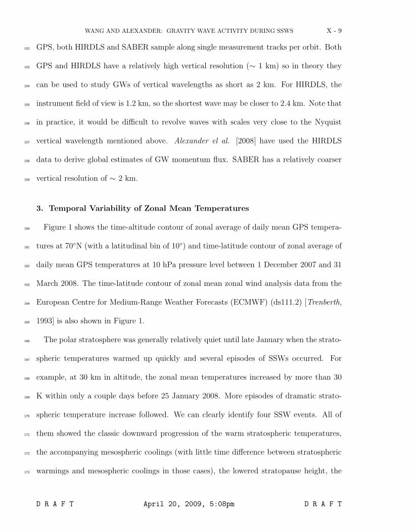
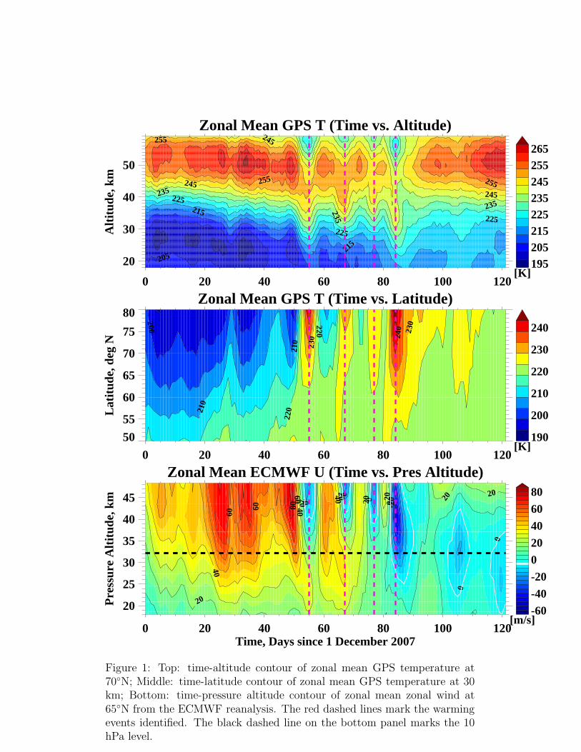
Figure 1 shows the time-altitude contour of zonal average of daily mean GPS tempera-160

tures at 70◦N (with a latitudinal bin of 10◦) and time-latitude contour of zonal average of161

daily mean GPS temperatures at 10 hPa pressure level between 1 December 2007 and 31162

March 2008. The time-latitude contour of zonal mean zonal wind analysis data from the163

European Centre for Medium-Range Weather Forecasts (ECMWF) (ds111.2) [Trenberth,164

1993] is also shown in Figure 1.165

The polar stratosphere was generally relatively quiet until late January when the strato-166

spheric temperatures warmed up quickly and several episodes of SSWs occurred. For167

example, at 30 km in altitude, the zonal mean temperatures increased by more than 30168

K within only a couple days before 25 January 2008. More episodes of dramatic strato-169

spheric temperature increase followed. We can clearly identify four SSW events. All of170

them showed the classic downward progression of the warm stratospheric temperatures,171

the accompanying mesospheric coolings (with little time difference between stratospheric172

warmings and mesospheric coolings in those cases), the lowered stratopause height, the173



reversed meridional temperature gradient, and the weakening (or even reversal) of the174

zonal wind. If we define the date of each event by the time when the meridional tem-175

perature gradient was positive and its value was maximum, the four SSWs occurred at176

25 January, 2 February, 16 February, and 23 February of 2008, respectively. Among the177

events, the 23 February one is a major event which is characterized by the reversal of the178

zonal wind at 10 hPa. The 25 January event is extraordinary in that its temporal change179

of temperatures is the largest among the four even though it is a minor one by the WMO180

definition. From the ECMWF analysis geopotential height data (not shown), these SSWs181

are mostly of the zonal wave-1 type, though also with some wave-2 component.182

Note that there could be large uncertainties in GPS temperature retrievals at upper183

levels (above ∼ 35 km) due to noise and the residual ionospheric effects [Kuo et al.,184

2004]. As noted by Kuo et al. [2004] though, the residual ionospheric effects in the GPS185

RO retrievals are the smallest during solar minimum at night time. Indeed, the time186

period considered in this study happens to correspond to a solar minimum. Also, we have187

conducted a separate zonal mean analysis of the night-time GPS data only and found188

that the results are largely the same as those reported here.189

The temperature retrievals at upper levels are also affected by a priori information190

used for the optimal estimation of bending angles and integration of the hydrostatic191

equation in the CDAAC GPS RO inversions. Specifically, the CDAAC uses the NCAR192

climatology described in Section 4 of [Randel et al., 2002] for the optimal estimation of193

bending angles and initialization of temperatures at 80 km to calculate the hydrostatic194

integral (Note that other GPS RO processing centers may use different climate models for195

those purposes.) The detailed descriptions of the optimal estimation of bending angles196



and the hydrostatic integral applied at the CDAAC are given by Kuo et al. [2004] and197

Lohmann [2005]. As a result of using a priori in the inversions, the temperature retrievals198

are a mixture of real neutral atmospheric signals, a priori information, and noise and199

the residual ionospheric effects (as discussed above), and the relative contribution from200

a priori increases significantly with altitude. Hence, the temperature retrievals at upper201

levels can be severely diluted by a priori information. Since the temporal variability of202

temperatures at upper levels exhibits a time scale of from several days up to ∼ a week203

during SSWs (Figure 1a) whereas the time scale of a priori used by the CDAAC is on the204

order of a month, the temporal variability of zonal mean temperatures at upper levels is205

likely due to true geophysical signals.206

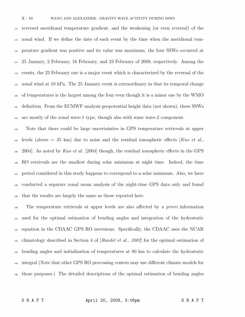
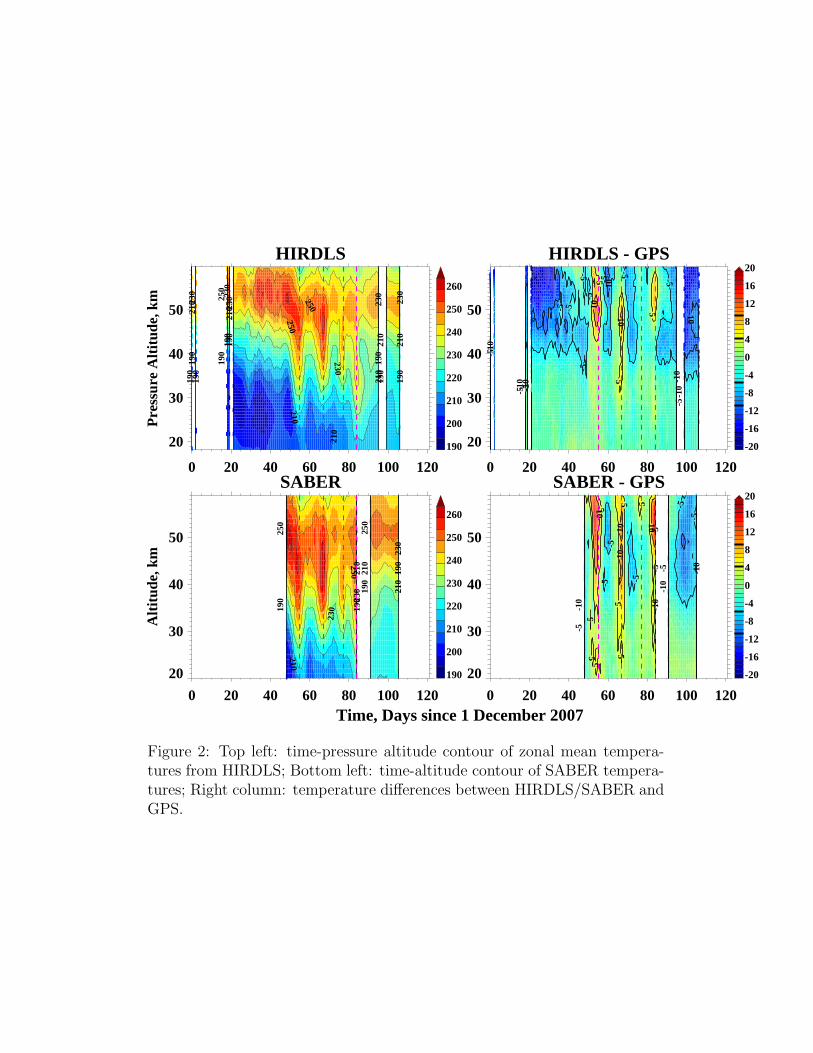
It would be interesting to compare the GPS results with those from HIRDLS and207

SABER (Figure 2). Since HIRDLS data are reported at pressure levels while SABER data208

are reported at geometric altitudes, the comparison is made at pressure and altitude levels209

for them, respectively (the GPS products include both altitude and pressure information).210

For the comparison with HIRDLS, we interpolate the GPS data to the HIRDLS pressure211

levels (which have an equivalent pressure altitude resolution of ∼ 0.672 km if a pressure212

scale height of 7 km is assumed) before calculating their differences shown in Figure 2b.213

For the comparison with SABER, we interpolate both the SABER and GPS data linearly214

to a regular vertical resolution of 1 km before calculating their differences shown in Figure215

2d. Note that there datasets used in the daily and zonal mean analysis shown in Figure216

2 have different spatial and local-time sampling. It is evident that all three datasets are217

capable of capturing the SSW events in the stratosphere and to first order the temporal218

variability of the GPS data at upper levels is generally similar to those from the other219



two datasets. Note that HIRDLS global mean temperatures are known to have a cold220

bias at upper levels [Gille et al., 2008]. This could possibly explain the overall warmer221

GPS temperatures than HIRDLS at upper levels. It is interesting to note that the GPS222

RO zonal mean temperatures are somewhat less sensitive to warmings than HIRDLS and223

SABER and this could be due to the optimization applied in the GPS RO inversions, that224

dilutes the neutral atmosphere signals with a priori as discussed above. Nevertheless, the225

comparison among the datasets suggests that the temporal variability of GPS zonal mean226

temperatures at upper levels is realistic.227

Finally, to assess the contribution of the real neutral atmospheric signals to the GPS228

temperature retrievals used in this study, we analyze the “zmwv” parameter in the229

CDAAC products. “zmwv” is the median height of the weighting vector for the ob-230

servational bending angle and at this height there is 50% of a priori in the optimized231

bending angle (Sergey Sokolovskiy, personal communication). This parameter varies with232

each individual RO occultation and for the occultations used in the analysis in Figure233

1a, it varies mostly between 40 and 50 km with a mean value of ∼ 44 km. We have234

also noticed that the value of “zmwv” is generally larger at high latitudes in winter (not235

shown). This factor together with the better spatial coverage of the GPS RO data in the236

polar regions than other satellite data (as described in Section 2) makes the GPS RO data237

valuable for studying the polar middle atmosphere.238

4. Temporal Variability of Gravity Wave Amplitude

As mentioned in Section 2, both GPS and HIRDLS have a rather good vertical reso-239

lution, so they can be used to study small-scale phenomena such as GWs. GW analysis240

depends on the extraction of GW perturbations, i.e., the removal of the “background”.241



Previous studies estimated GW temperature perturbations by applying a vertical wave-242

length (λz) filter directly to individual GPS temperature profiles [Tsuda et al., 2000;243

Ratnam et al., 2004; de la Torre et al., 2004; Baumgaertner and McDonald, 2007]. In244

fact, large-scale waves such as Kelvin waves can have similar λz as GWs. For example,245

Holton et al. [2001] identified from radiosonde data Kelvin waves of zonal wavenumber 2246

and 4 with vertical wavelength of ∼ 4.5 km and 3-4.5 km, respectively. Therefore, filtering247

temperature profiles with respect to λz alone does not clearly separate global-scale waves248

and GW signals. The combined COSMIC and CHAMP data provide nearly ten times249

more daily profiles than previous GPS missions, thus giving us the opportunity to define250

the background temperature on the basis of horizontal scale and to separate the GWs251

from the global-scale waves on this basis.252

We obtain GW perturbations using the following procedure (which is analogous to253

Alexander et al., 2008). First, each profile is interpolated in altitude to a regular 200-254

m resolution (which is oversampling for both GPS and HIRDLS). Next, each day’s255

profiles are gridded to 15◦ × 10◦ longitude and latitude resolution. The S-transform256

is performed as a function of longitude for each latitude and each altitude, giving zonal257

wavenumber 0-12 as a function of longitude. Note that the S-transform is a continuous258

wavelet-like analysis [Stockwell et al., 1996] that uses an absolute phase reference, and the259

longitudinal integral of the transform recovers the Fourier transform. In this study we260

reconstruct zonal wavenumbers 0-6 to define the “large-scale” temperature variation. This261

large scale, interpolated back to the positions of the original profiles, is subtracted leaving262

perturbations with horizontal fluctuations shorter than wavenumber 6. We have tested263

the sensitivity of the analysis results using different cut-off zonal wavenumbers ranging264



from 3 to 10 (whenever the data spatial coverage allows this) and have found that the265

major results reported here remain largely the same. Note that the above procedure to266

derive GW background profiles neglects any time variations of large-scale waves within267

one day. Finally, we derive GW temperature amplitudes as a function of altitude from268

the temperature perturbations using the S-transform.269

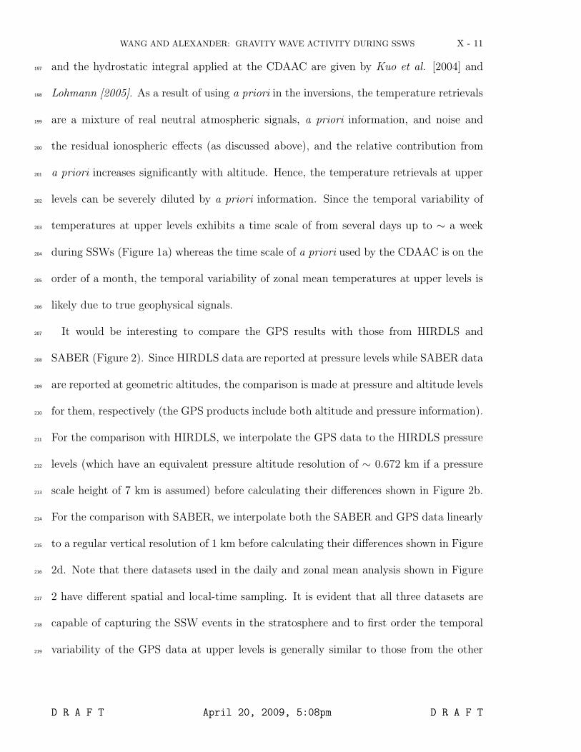
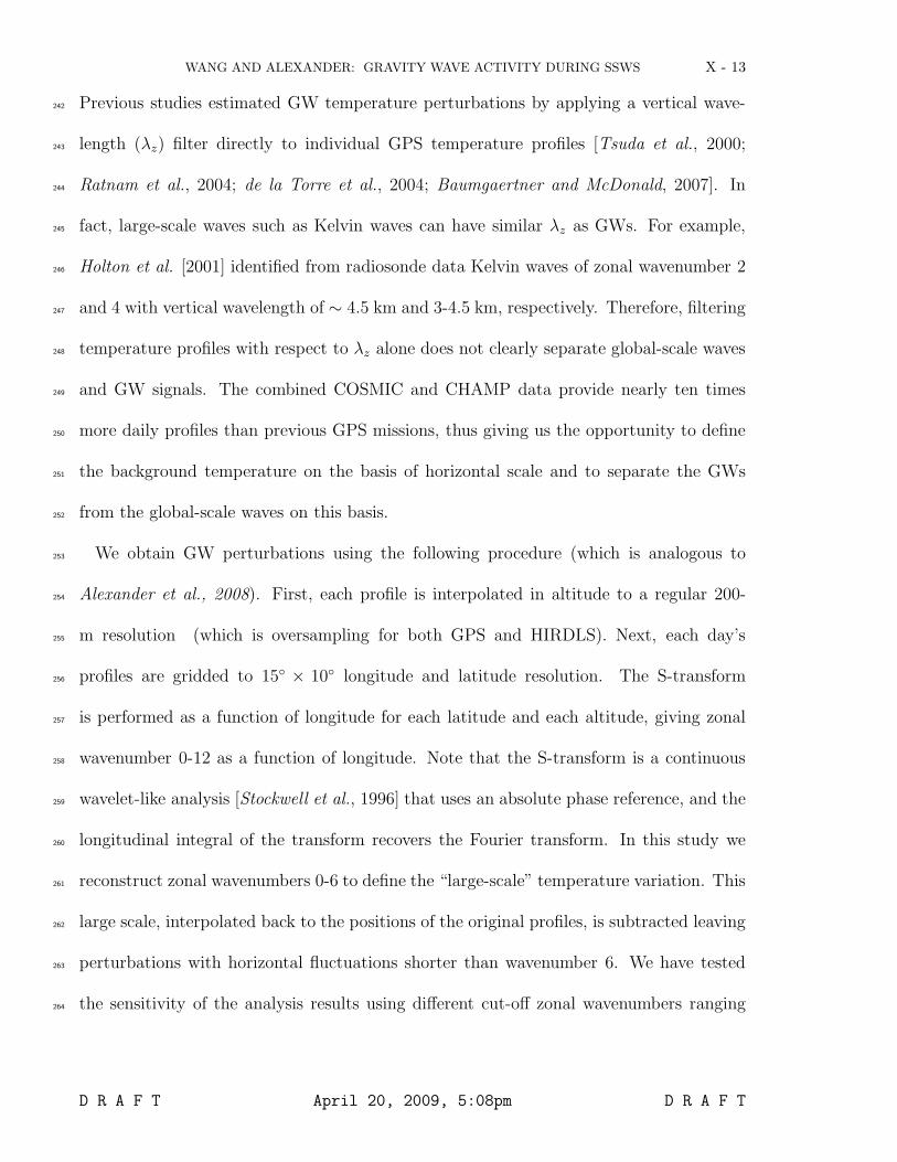
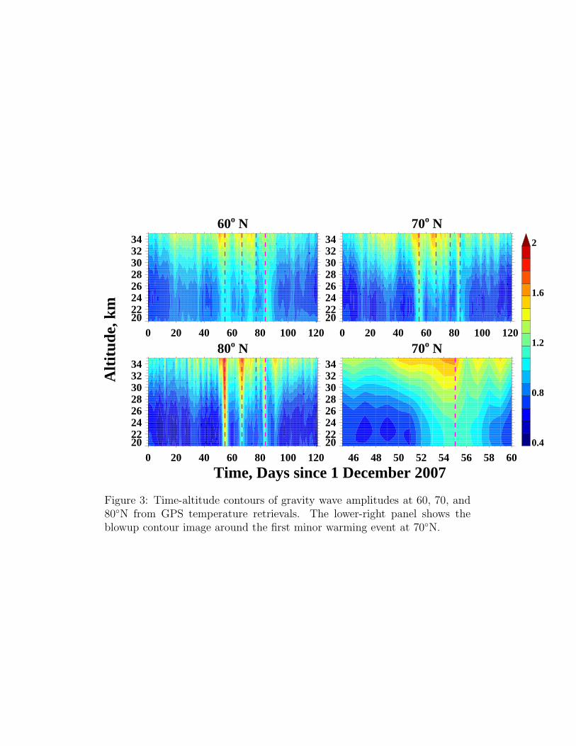
Figure 3 shows the time (daily)-altitude contours of zonal averaged GW temperature270

amplitudes at high latitudes. Evidently, there were enhancements of GW activity in the271

stratosphere during SSWs. At 70◦N, for example, GW temperature amplitude increased272

by a factor of 3 on 25 January 2008 in comparison to the time when the atmosphere was273

less disturbed during December 2007 and early January 2008. GW amplitudes were also274

smaller after the late February major warming event when the polar middle atmosphere275

started to transition from the winter to summer state. In the 25 January event, for in-276

stance, there was also a downward progression of GW signals associated with the warming277

event (Figure 3d).278

As mentioned in the Introduction, the enhancement of GW activity during SSWs has279

been reported in previous studies [e.g., Duck et al., 1998; Ratnam et al., 2004]. It is280

interesting though that the timing of GW enhancement was very close with that of the281

SSWs in the 2007/08 Northern Hemisphere winter (generally within 1 or 2 days) whereas282

Ratnam et al. [2004] reported enhanced GW potential energy appearing 10 days earlier283

than the major Southern Hemisphere SSW in late winter/spring of 2002.284

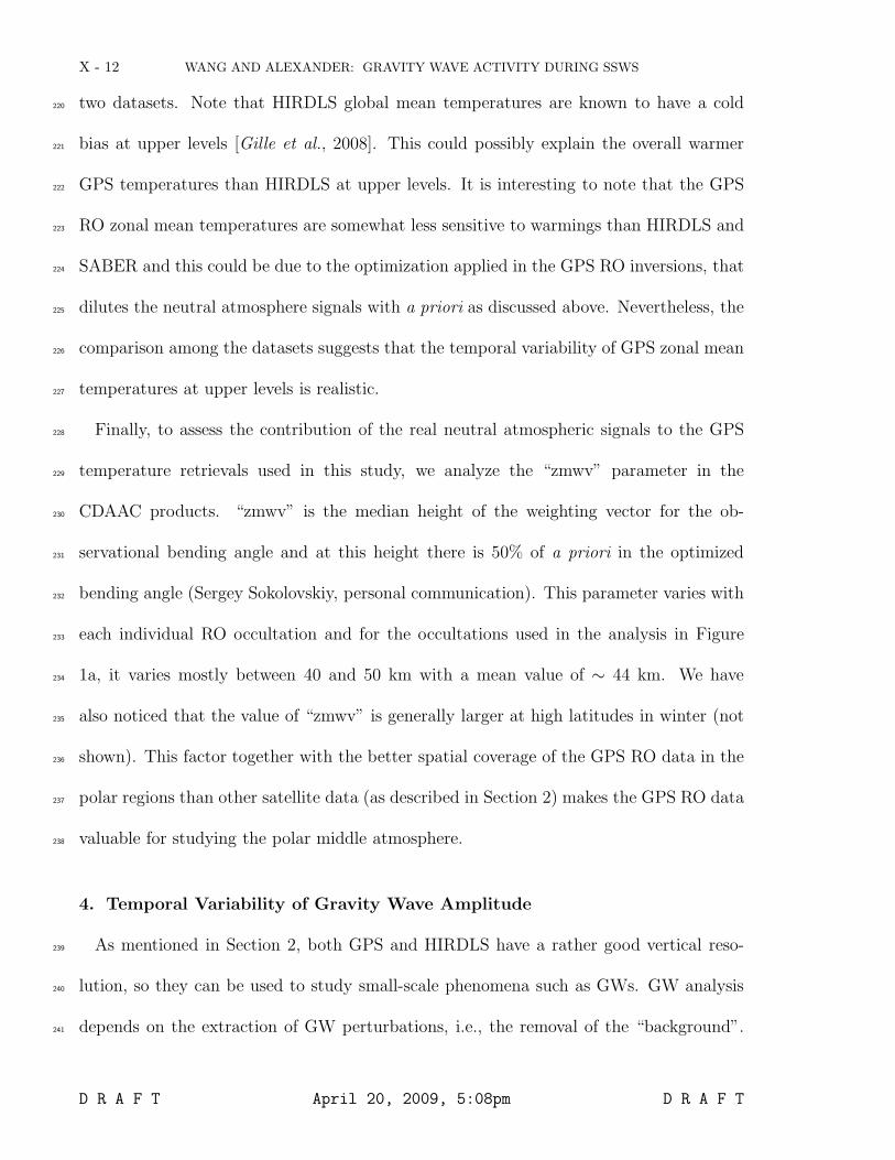
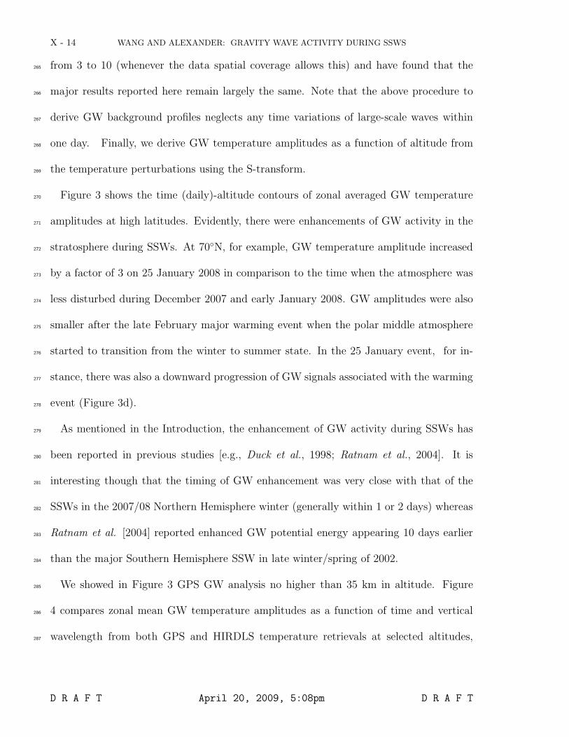
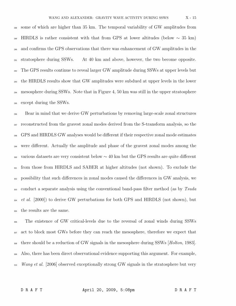
We showed in Figure 3 GPS GW analysis no higher than 35 km in altitude. Figure285

4 compares zonal mean GW temperature amplitudes as a function of time and vertical286

wavelength from both GPS and HIRDLS temperature retrievals at selected altitudes,287



some of which are higher than 35 km. The temporal variability of GW amplitudes from288

HIRDLS is rather consistent with that from GPS at lower altitudes (below ∼ 35 km)289

and confirms the GPS observations that there was enhancement of GW amplitudes in the290

stratosphere during SSWs. At 40 km and above, however, the two become opposite.291

The GPS results continue to reveal larger GW amplitude during SSWs at upper levels but292

the HIRDLS results show that GW amplitudes were subdued at upper levels in the lower293

mesosphere during SSWs. Note that in Figure 4, 50 km was still in the upper stratosphere294

except during the SSWs.295

Bear in mind that we derive GW perturbations by removing large-scale zonal structures296

reconstructed from the gravest zonal modes derived from the S-transform analysis, so the297

GPS and HIRDLS GW analyses would be different if their respective zonal mode estimates298

were different. Actually the amplitude and phase of the gravest zonal modes among the299

various datasets are very consistent below ∼ 40 km but the GPS results are quite different300

from those from HIRDLS and SABER at higher altitudes (not shown). To exclude the301

possibility that such differences in zonal modes caused the differences in GW analysis, we302

conduct a separate analysis using the conventional band-pass filter method (as by Tsuda303

et al. [2000]) to derive GW perturbations for both GPS and HIRDLS (not shown), but304

the results are the same.305

The existence of GW critical-levels due to the reversal of zonal winds during SSWs306

act to block most GWs before they can reach the mesosphere, therefore we expect that307

there should be a reduction of GW signals in the mesosphere during SSWs [Holton, 1983].308

Also, there has been direct observational evidence supporting this argument. For example,309

Wang et al. [2006] observed exceptionally strong GW signals in the stratosphere but very310



week GW signals in the mesosphere in the course of an SSW event during the winter311

MaCWAVE campaign. Thus, we have more confidence in the HIRDLS results at upper312

levels, and it is likely that the small-scale variability shown in the GPS data above 35 km313

might be due to the GPS retrieval uncertainty at upper levels. The residual ionospheric314

effects are normally the largest source for GPS temperature retrieval uncertainties at high315

altitudes [Kuo et al., 2004]. However, a separate GW analysis using only the night-time316

GSP data to minimize the residual ionospheric effects still shows the same seemingly317

erroneous temporal variability at upper levels. Also, if the small-scale variability is noise,318

it is unclear why noise would increase during SSW events. Therefore further studies are319

needed to pinpoint the underlying causes of the GPS retrieval uncertainty at upper levels.320

5. Geographic Variability of Gravity Wave Amplitude

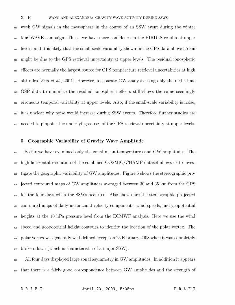
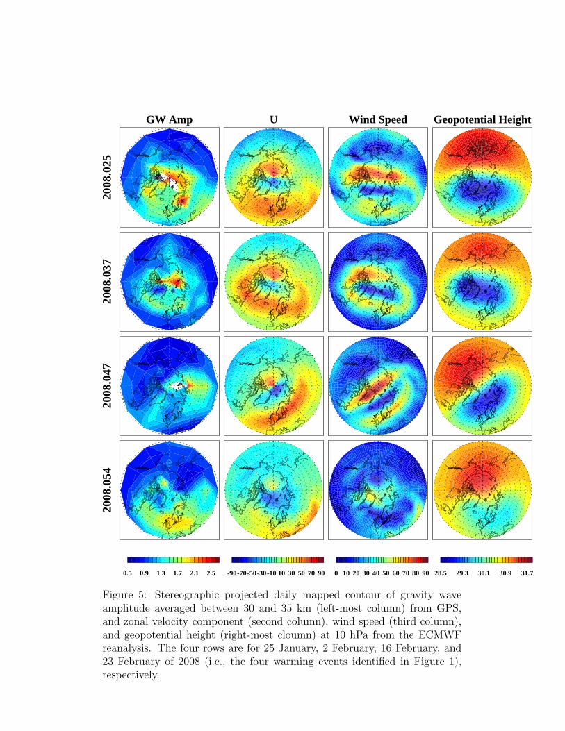
So far we have examined only the zonal mean temperatures and GW amplitudes. The321

high horizontal resolution of the combined COSMIC/CHAMP dataset allows us to inves-322

tigate the geographic variability of GW amplitudes. Figure 5 shows the stereographic pro-323

jected contoured maps of GW amplitudes averaged between 30 and 35 km from the GPS324

for the four days when the SSWs occurred. Also shown are the stereographic projected325

contoured maps of daily mean zonal velocity components, wind speeds, and geopotential326

heights at the 10 hPa pressure level from the ECMWF analysis. Here we use the wind327

speed and geopotential height contours to identify the location of the polar vortex. The328

polar vortex was generally well-defined except on 23 February 2008 when it was completely329

broken down (which is characteristic of a major SSW).330

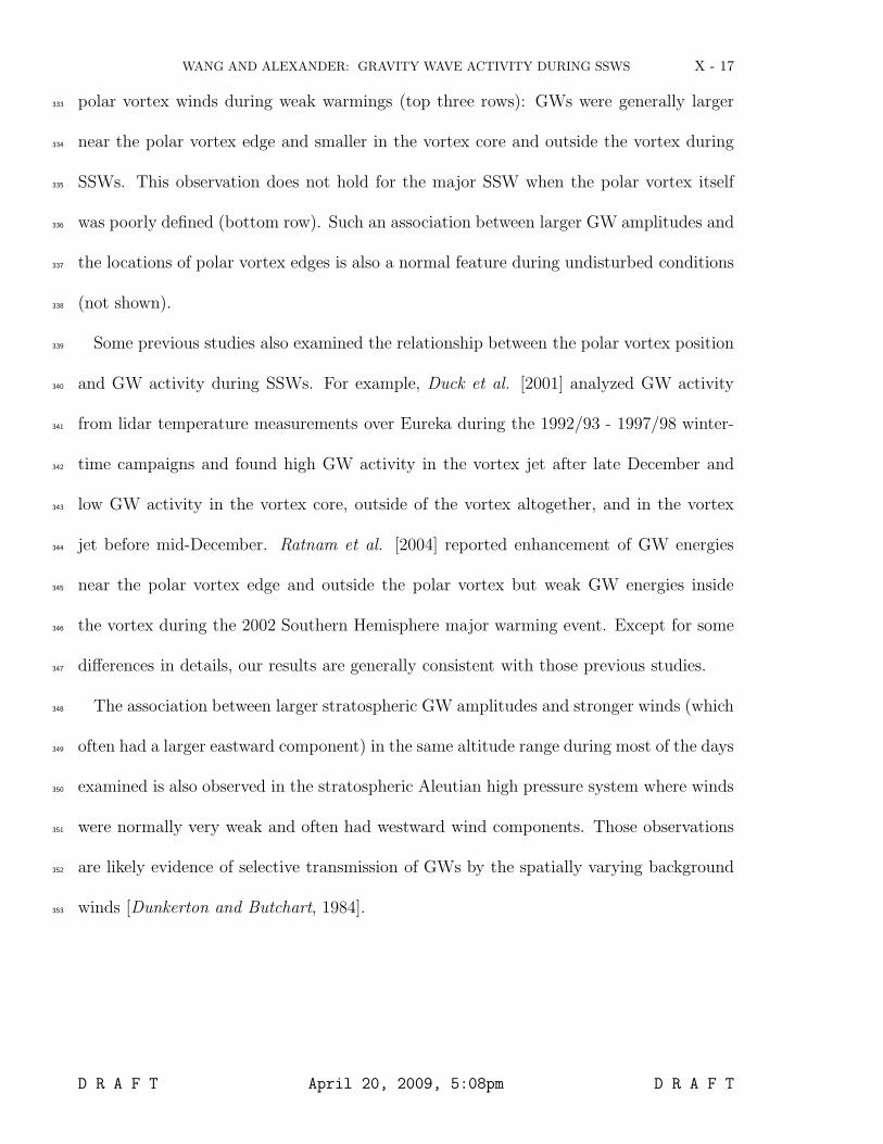
All four days displayed large zonal asymmetry in GW amplitudes. In addition it appears331

that there is a fairly good correspondence between GW amplitudes and the strength of332



polar vortex winds during weak warmings (top three rows): GWs were generally larger333

near the polar vortex edge and smaller in the vortex core and outside the vortex during334

SSWs. This observation does not hold for the major SSW when the polar vortex itself335

was poorly defined (bottom row). Such an association between larger GW amplitudes and336

the locations of polar vortex edges is also a normal feature during undisturbed conditions337

(not shown).338

Some previous studies also examined the relationship between the polar vortex position339

and GW activity during SSWs. For example, Duck et al. [2001] analyzed GW activity340

from lidar temperature measurements over Eureka during the 1992/93 - 1997/98 winter-341

time campaigns and found high GW activity in the vortex jet after late December and342

low GW activity in the vortex core, outside of the vortex altogether, and in the vortex343

jet before mid-December. Ratnam et al. [2004] reported enhancement of GW energies344

near the polar vortex edge and outside the polar vortex but weak GW energies inside345

the vortex during the 2002 Southern Hemisphere major warming event. Except for some346

differences in details, our results are generally consistent with those previous studies.347

The association between larger stratospheric GW amplitudes and stronger winds (which348

often had a larger eastward component) in the same altitude range during most of the days349

examined is also observed in the stratospheric Aleutian high pressure system where winds350

were normally very weak and often had westward wind components. Those observations351

are likely evidence of selective transmission of GWs by the spatially varying background352

winds [Dunkerton and Butchart, 1984].353



6. Mechanism for Stratospheric Gravity Wave Enhancements during SSWs

Figures 3 and 4 showed that GW amplitudes in the stratosphere were generally en-

hanced during SSWs. Such enhancements could be explained to some extent by the GW

propagation considerations. During SSWs, the zonal wind reversal (or weakening) could

refract GWs arising from the lower atmosphere in such a way that more waves could

be observed by GPS and HIRDLS in the stratosphere (i.e., the so-called observational

window effect introduced by Alexander [1998]). As the simplest illustration of this mech-

anism, we estimate the vertical wavelength of a stationary GW at the 10 hPa pressure

level using the following formula

λz = 2πu

N(1)

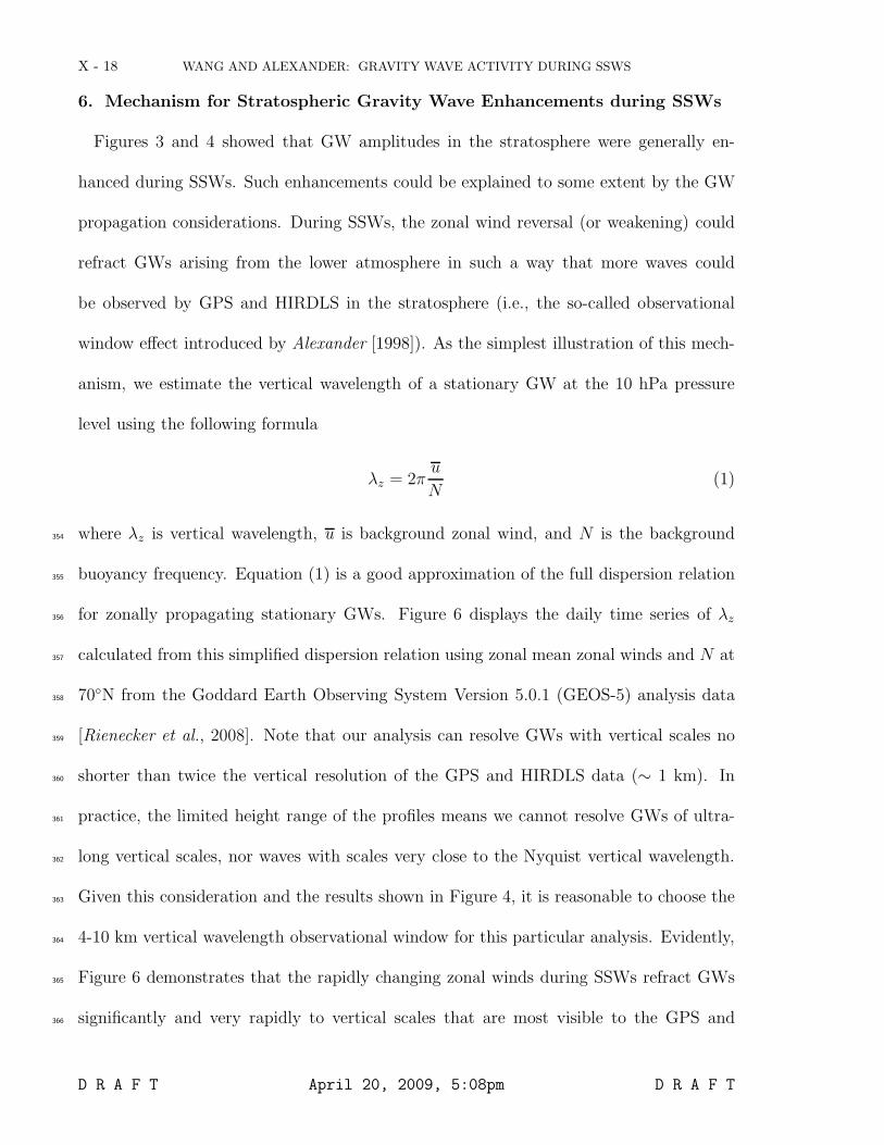
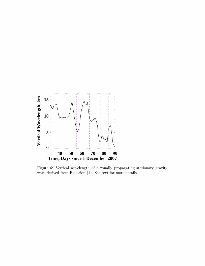
where λz is vertical wavelength, u is background zonal wind, and N is the background354

buoyancy frequency. Equation (1) is a good approximation of the full dispersion relation355

for zonally propagating stationary GWs. Figure 6 displays the daily time series of λz356

calculated from this simplified dispersion relation using zonal mean zonal winds and N at357

70◦N from the Goddard Earth Observing System Version 5.0.1 (GEOS-5) analysis data358

[Rienecker et al., 2008]. Note that our analysis can resolve GWs with vertical scales no359

shorter than twice the vertical resolution of the GPS and HIRDLS data (∼ 1 km). In360

practice, the limited height range of the profiles means we cannot resolve GWs of ultra-361

long vertical scales, nor waves with scales very close to the Nyquist vertical wavelength.362

Given this consideration and the results shown in Figure 4, it is reasonable to choose the363

4-10 km vertical wavelength observational window for this particular analysis. Evidently,364

Figure 6 demonstrates that the rapidly changing zonal winds during SSWs refract GWs365

significantly and very rapidly to vertical scales that are most visible to the GPS and366



HIRDLS observations. The estimated vertical wavelength for the third event is shorter367

than 4 km but still longer than the Nyquist vertical wavelength.368

There is generally large zonal asymmetry in zonal winds in the polar winter middle369

atmosphere and such zonal asymmetry can lead to the so-called GW selective transmission370

effects discussed by Dunkerton and Butchart [1984]. Hence, we conduct a GW ray-tracing371

experiment to see how both temporally and longitudinally varying zonal winds during372

SSWs could affect GWs that fall into the observational window of the GPS and HIRDLS373

data. In this experiment, we launch rays at an altitude of 10 km along the 70◦N latitude374

band with a longitudinal interval of 5◦. We use a constant source spectra with zonal phase375

speed ranging from -10 to 10 ms−1 with a resolution of 0.2 ms−1. We choose such a narrow376

band of phase speed centered around zero because Alexander and Rosenlof [2003] argued377

that the GW source spectra in extratropics should be quasi-stationary in winter and fall378

as constrained from satellite observations. The source spectra horizontal wavelength is379

taken to be 300 km, being close to the statistics of GW parameters reported by Wang et380

al. [2005]. The horizontal resolution of GPS RO temperature retrieval is ∼ 150 km along381

the line-of-sight of the occultation path and ∼ an order of magnitude small across the382

path. Smoothed daily mean GEOS-5 analysis data are used to represent the background383

atmosphere through which the waves are propagating. We use the Gravity-wave Regional384

Or Global RAy Tracer (GROGRAT) [Marks and Eckermann, 1995] as the GW ray-tracing385

solver. GROGRAT is capable of performing 4-D GW ray-tracing. For simplicity, only386

vertical propagation is considered in this experiment.387

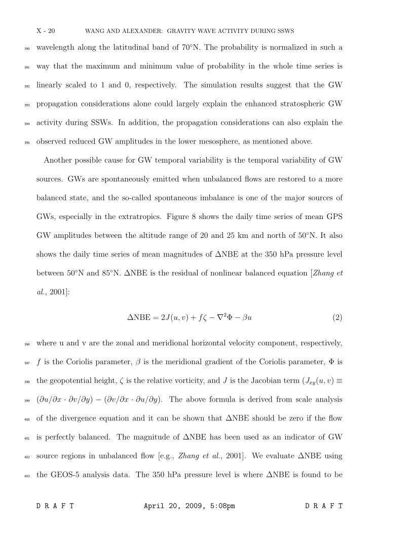
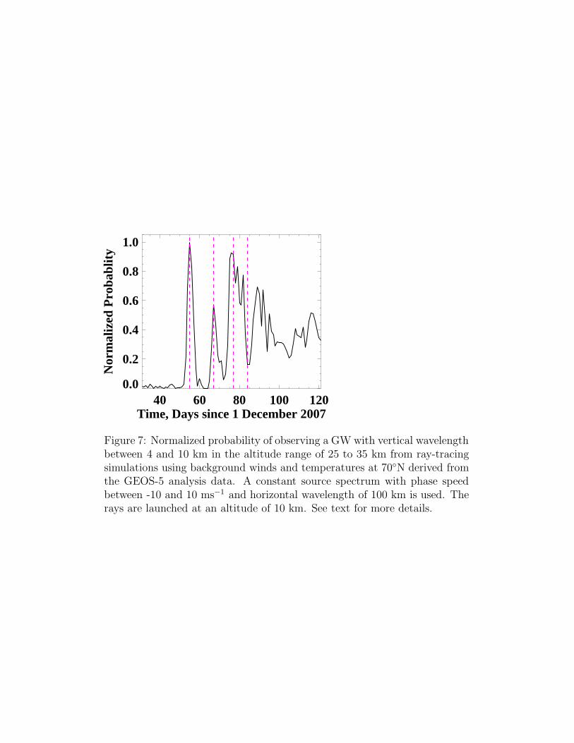
Figure 7 shows the time series of the normalized probability of observing a GW in388

the altitude range of 25 to 35 km in the observational window of 4-10 km in vertical389



wavelength along the latitudinal band of 70◦N. The probability is normalized in such a390

way that the maximum and minimum value of probability in the whole time series is391

linearly scaled to 1 and 0, respectively. The simulation results suggest that the GW392

propagation considerations alone could largely explain the enhanced stratospheric GW393

activity during SSWs. In addition, the propagation considerations can also explain the394

observed reduced GW amplitudes in the lower mesosphere, as mentioned above.395

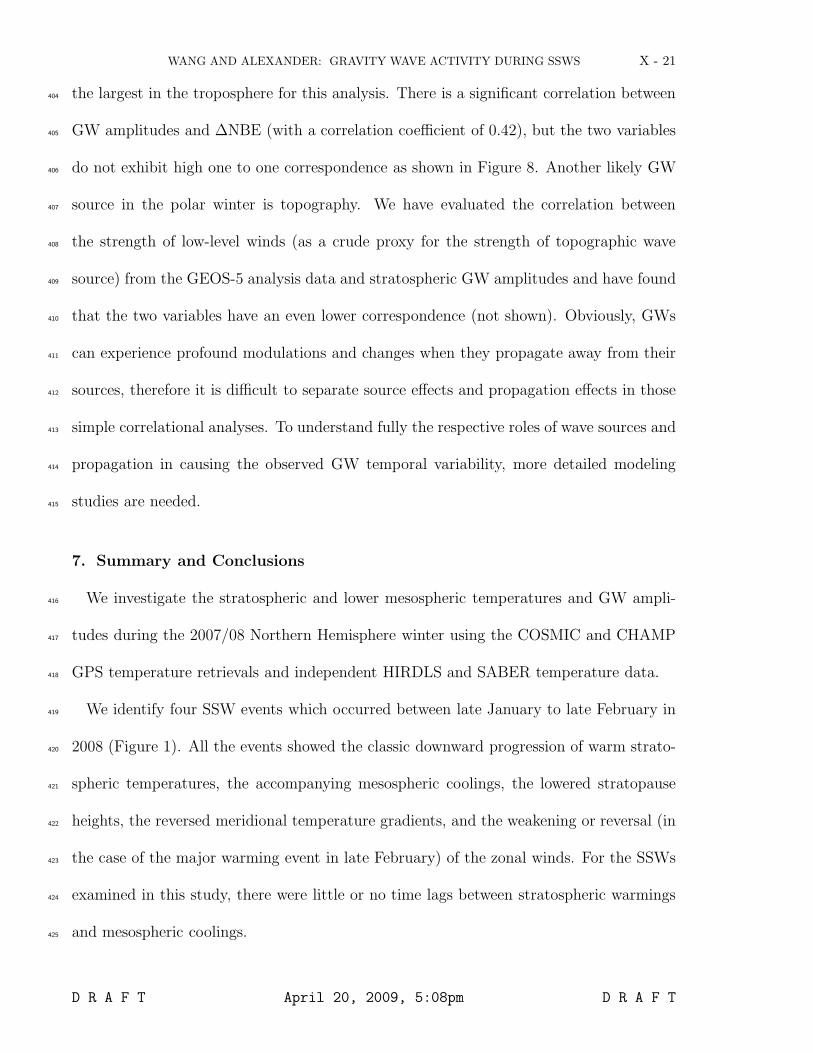
Another possible cause for GW temporal variability is the temporal variability of GW

sources. GWs are spontaneously emitted when unbalanced flows are restored to a more

balanced state, and the so-called spontaneous imbalance is one of the major sources of

GWs, especially in the extratropics. Figure 8 shows the daily time series of mean GPS

GW amplitudes between the altitude range of 20 and 25 km and north of 50◦N. It also

shows the daily time series of mean magnitudes of ∆NBE at the 350 hPa pressure level

between 50◦N and 85◦N. ∆NBE is the residual of nonlinear balanced equation [Zhang et

al., 2001]:

∆NBE = 2J (u, v) + fζ −∇2Φ − βu (2)

where u and v are the zonal and meridional horizontal velocity component, respectively,396

f is the Coriolis parameter, β is the meridional gradient of the Coriolis parameter, Φ is397

the geopotential height, ζ is the relative vorticity, and J is the Jacobian term (Jxy(u, v) ≡398

(∂u/∂x · ∂v/∂y) − (∂v/∂x · ∂u/∂y). The above formula is derived from scale analysis399

of the divergence equation and it can be shown that ∆NBE should be zero if the flow400

is perfectly balanced. The magnitude of ∆NBE has been used as an indicator of GW401

source regions in unbalanced flow [e.g., Zhang et al., 2001]. We evaluate ∆NBE using402

the GEOS-5 analysis data. The 350 hPa pressure level is where ∆NBE is found to be403



the largest in the troposphere for this analysis. There is a significant correlation between404

GW amplitudes and ∆NBE (with a correlation coefficient of 0.42), but the two variables405

do not exhibit high one to one correspondence as shown in Figure 8. Another likely GW406

source in the polar winter is topography. We have evaluated the correlation between407

the strength of low-level winds (as a crude proxy for the strength of topographic wave408

source) from the GEOS-5 analysis data and stratospheric GW amplitudes and have found409

that the two variables have an even lower correspondence (not shown). Obviously, GWs410

can experience profound modulations and changes when they propagate away from their411

sources, therefore it is difficult to separate source effects and propagation effects in those412

simple correlational analyses. To understand fully the respective roles of wave sources and413

propagation in causing the observed GW temporal variability, more detailed modeling414

studies are needed.415

7. Summary and Conclusions

We investigate the stratospheric and lower mesospheric temperatures and GW ampli-416

tudes during the 2007/08 Northern Hemisphere winter using the COSMIC and CHAMP417

GPS temperature retrievals and independent HIRDLS and SABER temperature data.418

We identify four SSW events which occurred between late January to late February in419

2008 (Figure 1). All the events showed the classic downward progression of warm strato-420

spheric temperatures, the accompanying mesospheric coolings, the lowered stratopause421

heights, the reversed meridional temperature gradients, and the weakening or reversal (in422

the case of the major warming event in late February) of the zonal winds. For the SSWs423

examined in this study, there were little or no time lags between stratospheric warmings424

and mesospheric coolings.425



We notice a large increase of GW amplitudes at high latitudes in the stratosphere426

during SSWs in the 2007/08 Northern Hemisphere winter and the timing of the GW427

enhancements with respect to SSWs was generally very close (within a couple days at428

most) (Figures 3-4). Ratnam et al. [2004] also noted enhanced GW energies during an429

SSW event in the Southern Hemisphere in 2002 but the stratospheric GW energy spike430

occurred ∼ ten days earlier than the warming event. The enhancements of stratospheric431

GW activity during SSWs can be primarily explained by GW propagation considerations.432

During SSWs, the zonal wind reversal (or weakening) could refract GWs arising from the433

lower atmosphere in such a way that more waves could be observed by GPS and HIRDLS434

in the stratosphere. The simple vertical wavelength estimates (Figure 6) and GW ray435

tracing results (Figure 7) support this wave refraction interpretation. We also notice a436

decrease of GW amplitudes in the lower mesosphere during SSWs (above ∼ 35 km, as the437

stratopause is lowered during SSWs) (Figure 4). This reduction of GW activity is likely438

due to the existence of GW critical levels caused by the zonal wind weakening or reversal439

during SSWs, implying GW dissipation and drag on the mean flow at lower altitudes than440

during undisturbed conditions.441

Stratospheric GW amplitudes display large geographic variability. Consistent with some442

previous studies, GW amplitudes were generally larger at the polar vortex edge, and443

smaller in the vortex core and outside of the vortex. This association could be due to444

the possibility that strong polar vortex jet winds allow more transmission of GWs to this445

altitude range so that they can be discerned in the satellite data.446

As the first study to extend the usage of the COSMIC and CHAMP GPS temperature447

data up to 60 km in altitude, we compare the GPS analysis with independent HIRDLS and448



SABER temperature retrievals. We find that the temporal variability of the HIRDLS and449

SABER zonal mean temperatures generally agrees well with that of the GPS (Figures 1450

and 2) up to ∼ 60 km. This could have particular implications for polar atmospheric stud-451

ies because the GPS data have better coverage at very high latitudes (e.g., the COSMIC452

GPS occultations can routinely reach within 2◦ of the poles) than other satellite data such453

as HIRDLS and SABER. The GPS zonal mean temperatures are, however, somewhat less454

sensitive to warmings than HIRDLS and SABER. GW analysis from GPS is consistent455

with HIRDLS up to ∼ 35 km. At higher altitudes, there is indication that small-scale456

variability in the GPS data is questionable, though this needs to be investigated further457

in future studies.458

We finally note that there exist different types of SSW events with various characteris-459

tics and more observational and modeling studies are needed to gain a more comprehensive460

and thorough understanding of the relationship between the two phenomena, which has461

significant implications for improved understanding of both the middle and lower atmo-462

sphere.463

Acknowledgments.464

We appreciate the valuable discussions with Dr. Sergey Sokolovskiy at the University465

Corporation for Atmospheric Research on the CDAAC GPS RO inversions. We thank466

Dr. Viktoria Sofieva at the Finnish Meteorological Institute for helpful discussions on467

this manuscript. We would also like to thank the three anonymous reviewers for their468

constructive comments. This research was supported by the Climate and Large Scale469

Dynamics Program of the National Science Foundation grant ATM-0737692. Support for470

MJA was in part funded by NASA contract NNH06CD16C.471



References

Alexander, M. J., 1998: Interpretations of observed climatological patterns in strato-472

spheric gravity wave variance, J. Geophys. Res., 103, 8627-8640.473

Alexander, M. J., and K. H. Rosenlof, 2003: Gravity wave forcing in the stratosphere:474

Observational constraints from UARS and implications for parameterization in global475

models, J. Geophys. Res., 108, D19, 4597, doi:10.1029/2003JD003373.476

Alexander, M. J., J. Gille, C. Cavanaugh, M. Coffey, C. Craig, V. Dean, T. Eden, G.477

Francis, C. Halvorson, J. Hannigan, R. Khosravi, D. Kinneson, H. Lee, S. Massie, B.478

Nardi, A. Lambert, 2008: Global Estimates of Gravity Wave Momentum Flux from479

High Resolution Dynamics Limb Sounder (HIRDLS) Observations, J. Geophys. Res.,480

113, D15S18, doi:10.1029/2007JD008807.481

Alexander, S. P., T. Tsuda, Y. Kawatani, and M. Takahashi, 2008: Global distribu-482

tion of atmospheric waves in the equatorial upper troposphere and lower stratosphere:483

COSMIC observations of wave mean flow interactions, J. Geophys. Res., 113, D24115,484

doi:10.1029/2008JD010039.485

Andrews, D. G., J. R. Holton, and C. B. Leovy, 1987: Middle Atmospheric Dynamics.486

Academic Press, 489 pp.487

Baldwin, M. P., and T. J. Dunkerton, 2001: Stratospheric harbingers of anomalous488

weather regimes. Science, 294, 581-584.489

Baumgaertner, A. J. G, and A. J. McDonald, 2007: A gravity wave climatol-490

ogy for Antarctica compiled from Challenging Minisatellite Payload/Global Posi-491

tioning System (CHAMP/GPS) radio occultations, J. Geophys. Res., 112, D05103,492

doi:10.1029/2006JD007504.493



de la Torre, A., T. Tsuda, G. A. Hajj, and J. Wickert, 2004: A global distribution of494

the stratospheric gravity wave activity from GPS occultation profiles with SAC-C and495

CHAMP, J. Meteorol. Soc. Jpn., 82(1B), 407-417.496

Dowdy, A. J., R. A. Vincent, M. Tsutsumi, K. Igarashi, Y. Murayama, W . Singer,497

D. J. Murphy, and D. M. Riggin, 2007: polar mesosphere and lower thermosphere498

dynamics: 2. Response to sudden stratospheric warmings, J. Geophys. Res., 106, 112,499

doi:10.1029/2006JD008127.500

Duck, T. J., J. A. Whiteway, and A. I. Carswell, 1998: Lidar observations of gravity501

wave activity and Arctic stratospheric vortex core warming, Geophys. Res. Lett., 25,502

2813-2816.503

Duck, T. J., J. A. Whiteway, and A. I. Carswell , 2001: The gravity wave-arctic strato-504

spheric vortex interaction. J. Atmos. Sci., 58, 3581-3596.505

Dunkerton, T. J., and N. Butchart, 1984: Propagation and selective transmission of506

internal gravity waves in a sudden warming, J. Atmos. Sci., 41, 1443-1460.507

Garcia, R. R., and B. A. Boville, 1994: “Downward Control” of the mean meridional508

circulation and temperature distribution of the polar winter stratosphere, J. Atmos.509

Sci., 51, 2238-2245.510

Gille, J., et al., 2008: The High Resolution Dynamics Limb Sounder (HIRDLS):511

Experiment overview, results and temperature validation, J. Geophys. Res.,512

doi:10.1029/2007JD008824.513

Haynes, P. H., C. J. Marks, M. E. McIntyre, T. G. Shepherd, and K. P. Shine, 1991: On514

the “downward control” of extratropical diabatic circulations by eddy-induced mean515

zonal forces, J. Atmos. Sci., 48, 651-678.516



Hei, H., T. Tsuda, and T. Hirooka, 2008: Characteristics of atmospheric gravity wave517

activity in the polar regions revealed by GPS radio occultation data with CHAMP, J.518

Geophy. Res., 113, doi:10.1029/2007JD008938.519

Holton, J. R., 1983: The influence of gravity wave breaking on the general circulation of520

the middle atmosphere. J. Atmos. Sci., 40, 2497-2507.521

Holton, J. R., M. J. Alexander, and M. T. Boehm, 2001: Evidence for short vertical wave-522

length Kelvin waves in the Department of Energy-Atmospheric Radiation Measurement523

Nauru99 radiosonde data, J. Geophys. Res., 106, 20,125-20,129.524

Kuo, Y.-H., T.-K. Wee, S. Sokolovskiy, C. Rocken, W. Schreiner, D. Hunt, and R. A.525

Anthes, 2004: Inversion and error estimation of GPS radio occultation data, J. Meteorol.526

Soc. Jpn, 82, 507-531.527

Lohmann, M.S., 2005: Application of dynamical error estimation for statisti-528

cal optimization of radio occultation bending angles. Radio Sci., 40, RS3011,529

doi:10.1029/2004RS003117.530

Marks, C. J., and S. D. Eckermann, 1995: A three-dimensional nonhydrostatic ray-tracing531

model for gravity waves: Formulation and preliminary results for the middle atmo-532

sphere, J. Atmos. Sci., 52, 1959-1984.533

Matsuno, T., 1971: A dynamical model of the stratospheric sudden warmings. J. Atmos.534

Sci., 28, 1479-1494.535

Matsuno, T., and K. Nakamura, 1979: The Eulerian and Lagrangian-mean meridional536

circulations in the stratosphere at the time of a sudden warming. J. Atmos. Sci., 36,537

640-654.538



Mlynczak, M., and J. Russell, 1995: An overview of the SABER experiment for the539

TIMED mission, NASA Langley Research Center, Optical Remote Sensing of the At-540

mosphere, 2.541

Randel, W., M.-L. Chanin and C. Michaut., 2002: SPARC Intercomparison of Middle542

Atmosphere Climatologies, WCRP-116, WMO/TD-No.1142, SPARC Report No.3, 96543

pp.544

Ratnam, M. V., T. Tsuda, C. Jacobi, and Y. Aoyama, 2004: Enhancement545

of gravity wave activity observed during a major Southern Hemisphere strato-546

spheric warming by CHAMP/GPS measurements, Geophys. Res. Lett., 31, L16101,547

doi:10.1029/2004GL019789.548

Rienecker, M. M., et al., 2008: The GEOS-5 data assimilation system,549

documentation of versions 5.0.1, 5.1.0, and 5.2.0, Technical Report series550

on Global Modeling and Data Assimilation, NASA/TM-2008-104606, Vol. 27551

(http://gmao.gsfc.nasa.gov/pubs/docs/GEOS5 104606-Vol27.pdf).552

Rocken, C., Y.-H. Kuo, W. Schreiner, D. Hunt, S. Sokolovskiy, and C. McCormick, 2000:553

COSMIC system description, Terr. Atmos. Oceanic Sci., 11(1), 21-52.554

Stockwell, R. G., L. Mansinha, and R. P. Lowe, 1996: Localisation of the complex spec-555

trum: the S-transform, J. Assoc. Expl. Geophys., XVII, 99-114.556

Trenberth, K. E., 1992: Global Analyses from ECMWF and Atlas of 1000 to 10 mb557

Circulation Statistics. TN-373+STR, National Center for Atmospheric Research, 205558

pp.559

Tsuda, T., M. Nishida, C. Rocken, and R. H. Ware, 2000: A global morphology of gravity560

wave activity in the stratosphere revealed by the GPS occultation data (GPS/MET),561



J. Geophys. Res., 105, 7257-7273.562

Wang, L., D. C. Fritts, B. P. Williams, R. A. Goldberg, F. J. Schmidlin, and U. Blum,563

2006: Gravity waves in the middle atmosphere during the MaCWAVE winter campaign:564

Evidence of mountain wave critical level encounters, Ann. Geophys., 24, 1209-1226.565

Wang, L., M. A. Geller, and M. J. Alexander, 2005: Spatial and temporal variations of566

gravity wave parameters. Part I: Intrinsic frequency, wavelength, and vertical propaga-567

tion direction, J. Atmos. Sci., 62, 125-142.568

Ware, R., M. Exnet, D. Feng, M. Gorbunov, K. Hardy, B. Herman, Y. Kuo, T. Meehan, W.569

Melbourne, C. Rocken, W. Schreiner, S. Sokolovskiy, F. Solheim, X. Zhou, R. Anthes,570

S. Businger, and K. Trenberth, 1996: GPS sounding of the atmosphere: Preliminary571

results, Bull. Am. Meteorol. Soc., 77, 19-40.572

Yunck, T. P., G. F. Lindal, and C. H. Liu, 1988: The role of GPS in precise earth ob-573

servation, paper presented at the IEEE Position, Location and Navigation Symposium,574

Inst. of Electr. and Electron. Eng., Orlando, Fla., 29 Nov. to 2 Dec.575

Zhang, F., S. E. Koch, C. A. Davis, and M. L. Kaplan, 2001: Wavelet analysis and the576

governing dynamics of a large-amplitude gravity wave event along the East Coast of577

the United States, Q. J. R. Meteorol. Soc., 127, 2209-2245.578


Zonal Mean GPS T (Time vs. Altitude)

0 20 40 60 80 100 120

20

30

40

50

Alt

itud

e, k

m

20521

5

215225

225

225235

235

235 245

245

245 255

255

255

195205215225235245255265

[K]

Zonal Mean GPS T (Time vs. Latitude)

0 20 40 60 80 100 120

50

55

60

65

70

75

80

Lat

itud

e, d

eg N

200

210

210

220

220

230

230

240

190

200

210

220

230

240

[K]

Zonal Mean ECMWF U (Time vs. Pres Altitude)

0 20 40 60 80 100 120Time, Days since 1 December 2007

20

25

30

35

40

45

Pre

ssur

e A

ltit

ude,

km

-20

0

0

0

0 0

0

2020

20

20

20

20 20

40

40

40

60

60

6080

-60

-40

-20

0

20

40

60

80

[m/s]

Figure 1: Top: time-altitude contour of zonal mean GPS temperature at70◦N; Middle: time-latitude contour of zonal mean GPS temperature at 30km; Bottom: time-pressure altitude contour of zonal mean zonal wind at65◦N from the ECMWF reanalysis. The red dashed lines mark the warmingevents identified. The black dashed line on the bottom panel marks the 10hPa level.

HIRDLS

0 20 40 60 80 100 120

20

30

40

50

Pre

ssur

e A

ltit

ude,

km

190

190

190

190

190

190

190

190

190

210

210

210

210

210

210

210

230

230

230

230

230

230

250

250

250

190

200

210

220

230

240

250

260

HIRDLS - GPS

0 20 40 60 80 100 120

20

30

40

50

-10

-10

-10

-10

-10

-10

-10

-5 -5

-5

-5

-5

-5

-5

-5

-5

-5

-5

-5

5

5

5

10

10

-20

-16

-12

-8

-4

0

4

8

12

16

20

SABER

0 20 40 60 80 100 120

20

30

40

50

Alt

itud

e, k

m

190

190

190

190

210

210

210

210

230

230

230

250

250

250

190

200

210

220

230

240

250

260

SABER - GPS

0 20 40 60 80 100 120

20

30

40

50

-10

-10

-10

-10

-5

-5-5

-5

-5-5-5

-5

5 5

5

5

5

5

5 5

5

10

10

1010

-20

-16

-12

-8

-4

0

4

8

12

16

20

Time, Days since 1 December 2007

Figure 2: Top left: time-pressure altitude contour of zonal mean tempera-tures from HIRDLS; Bottom left: time-altitude contour of SABER tempera-tures; Right column: temperature differences between HIRDLS/SABER andGPS.

60o N

0 20 40 60 80 100 1202022242628303234

70o N

0 20 40 60 80 100 1202022242628303234

80o N

0 20 40 60 80 100 1202022242628303234

70o N

46 48 50 52 54 56 58 602022242628303234

0.4

0.8

1.2

1.6

2

Time, Days since 1 December 2007

Alt

itud

e, k

m

Figure 3: Time-altitude contours of gravity wave amplitudes at 60, 70, and80◦N from GPS temperature retrievals. The lower-right panel shows theblowup contour image around the first minor warming event at 70◦N.

GPS, 20 km

0 20 40 60 80 100 120456789

Days since 1 December 2007

Lz,

km

30 km

0 20 40 60 80 100 120456789

40 km

0 20 40 60 80 100 120456789

50 km

0 20 40 60 80 100 120456789

HIRDLS, 20 km

0 20 40 60 80 100 120456789

0.10.30.50.70.9

30 km

0 20 40 60 80 100 120456789

0.30.50.70.91.11.3

40 km

0 20 40 60 80 100 120456789

0.40.60.811.21.41.61.82

50 km

0 20 40 60 80 100 120456789

0.40.81.21.622.42.8

Figure 4: Time-vertical wavelength contour of zonal mean gravity wave am-plitude at 70◦ from GPS (left column) and HIRDLS (right column) at selectedaltitudes.

GW Amp U Wind Speed Geopotential Height20

08.0

2520

08.0

3720

08.0

47

0.5 0.9 1.3 1.7 2.1 2.5 -90-70-50-30-10 10 30 50 70 90 0 10 20 30 40 50 60 70 80 90 28.5 29.3 30.1 30.9 31.7

2008

.054

Figure 5: Stereographic projected daily mapped contour of gravity waveamplitude averaged between 30 and 35 km (left-most column) from GPS,and zonal velocity component (second column), wind speed (third column),and geopotential height (right-most cloumn) at 10 hPa from the ECMWFreanalysis. The four rows are for 25 January, 2 February, 16 February, and23 February of 2008 (i.e., the four warming events identified in Figure 1),respectively.

40 50 60 70 80 90Time, Days since 1 December 2007

0

5

10

15

Ver

tica

l Wav

elen

gth,

km

Figure 6: Vertical wavelength of a zonally propagating stationary gravitywave derived from Equation (1). See text for more details.

40 60 80 100 120Time, Days since 1 December 2007

0.0

0.2

0.4

0.6

0.8

1.0

Nor

mal

ized

Pro

babl

ity

Figure 7: Normalized probability of observing a GW with vertical wavelengthbetween 4 and 10 km in the altitude range of 25 to 35 km from ray-tracingsimulations using background winds and temperatures at 70◦N derived fromthe GEOS-5 analysis data. A constant source spectrum with phase speedbetween -10 and 10 ms−1 and horizontal wavelength of 100 km is used. Therays are launched at an altitude of 10 km. See text for more details.

gravity wave activity during stratospheric sudden warmings...

Documents