gröbner bases techniques in cryptography · gröbner bases techniques in cryptography ludovic...

Gröbner bases techniques in Cryptography

Ludovic Perret

SALSALIP6, Université Paris 6 & INRIA Paris-Rocquencourt

[email protected]

Plan

1 Algebraic Cryptanalysis

2 MinRank

3 Solving MinRank (Faugère/Levy/Perret, CRYPTO’08)Kipnis-ShamirExperimental ResultsTheoretical Analysis (Faugère, Safey El Din,Spaenlehauer, ISSAC’10).

General Context

C.E. Shannon

Communication Theory of Secrecy Systems (1949)

“Breaking a good cipher should require as much work assolving a system of simultaneous equations in a large numberof unknowns of a complex type.”

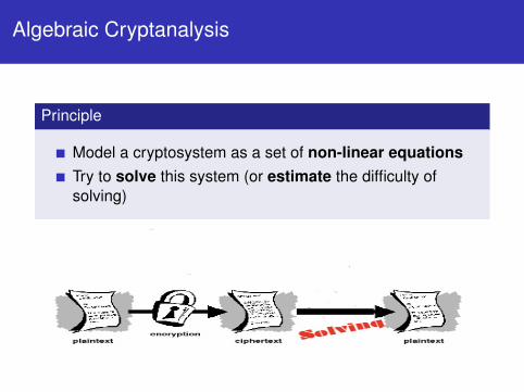
Algebraic Cryptanalysis

Principle

Model a cryptosystem as a set of non-linear equationsTry to solve this system (or estimate the difficulty ofsolving)

Approach

Difficulties

Model a cryptosystemas a set of non-linearequations

“universal" approach(PoSSo is NP-Hard)⇒ several models are

possible !!!

Solving⇒ Minimize the number

of variables/degree⇒ Maximize the number

of equations

Specificity

Solving algebraic systems :Gröbner bases

Gröbner Basis

K : finite field K[x1, . . . , xn] : polynomial ring in n variables.

Linear Systems

{x1 + x2 − 1 = 0x1 − x2 = 0

Polynomial Systems

Gröbner Basis


Linear Systems

{x1 + x2 − 1 = 0x1 − x2 = 0

Polynomial Systems

{x1x2 − x2

2 = 0,x2

1 − x1 = 0

Gröbner Basis


Linear Systems

`1(x1, . . . , xn) = 0`2(x1, . . . , xn) = 0

...`m(x1, . . . , xn) = 0

Polynomial Systems

f1(x1, . . . , xn) = 0f2(x1, . . . , xn) = 0

...fm(x1, . . . , xn) = 0

Gröbner Basis


Linear Systems

`1(x1, . . . , xn) = 0`2(x1, . . . , xn) = 0

...`m(x1, . . . , xn) = 0

V = VectK(`1, . . . , `m)

Triangular/diagonalbasis of V

Polynomial Systems

f1(x1, . . . , xn) = 0f2(x1, . . . , xn) = 0

...fm(x1, . . . , xn) = 0

Gröbner Basis


Linear Systems

`1(x1, . . . , xn) = 0`2(x1, . . . , xn) = 0

...`m(x1, . . . , xn) = 0

V = VectK(`1, . . . , `m)

Triangular/diagonalbasis of V

Polynomial Systems

f1(x1, . . . , xn) = 0f2(x1, . . . , xn) = 0

...fm(x1, . . . , xn) = 0

Ideal I = 〈f1, . . . , fm〉 =

{ m∑i=1

fiui | ui ∈ K[x1, . . . , xn]}.

Gröbner basis of I ⊂ K[x1, . . . , xn]

Gröbner Basis

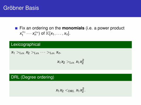
Fix an ordering on the monomials (i.e. a power productxα1

1 · · · xαnn ) of K[x1, . . . , xn].

Lexicographical

x1 >Lex x2 >Lex · · · >Lex xn.

x1x2 >Lex x1x22

Gröbner Basis


1 · · · xαnn ) of K[x1, . . . , xn].

Lexicographical

x1 >Lex x2 >Lex · · · >Lex xn.

x1x2 >Lex x1x22

DRL (Degree ordering)

x1x2 <DRL x1x22 .

Gröbner Basis


1 · · · xαnn ) of K[x1, . . . , xn].

Definition (Buchberger 1965/1976)

Let I be an ideal of K[x1, . . . , xn]. A subset G ⊂ I is a Gröbnerbasis if:

∀f ∈ I, ∃g ∈ G s. t. LM(g) divides LM(f ).

LEX Gröbner Basis

Problem

f1(x1, . . . , xn), . . . , fm(x1, . . . , xn) ∈ K[x1, . . . , xn]

Compute VK(f1, . . . , fm) ={z = (z1, . . . , zn) ∈ Kn | f1(z) = 0, . . . , fm(z) = 0

}

LEX Gröbner Basis

Problem

f1(x1, . . . , xn), . . . , fm(x1, . . . , xn) ∈ K[x1, . . . , xn]

Compute VK(f1, . . . , fm) ={z = (z1, . . . , zn) ∈ Kn | f1(z) = 0, . . . , fm(z) = 0

}Lemma

Let I =⟨f1, . . . , fm, x

p1 − x1, . . . , x

pn − xn〉, with p = Char(K).

A LEX Gröbner basis of a zero-dimensional system is alwaysas follows :{

g1(x1),g2(x1, x2), . . . ,gk2(x1, x2),gk2+1(x1, x2, x3), . . . , . . .}

Change of ordering

Computing LEX is much more slower than computing DRL

J.-C. Faugère , P. Gianni, D. Lazard, and T. Mora.Efficient Computation of Zero-dimensional Gröbner Basesby Change of Ordering.J. Symb. Comp., 1993.

Fact

D : the nb. of zeroes (with multiplicities) of I ⊂ K[x1, . . . , xn].FGLM computes a DRL-Gröbner basis of I knowing a LEXGröbner basis in :

O(nD3).

Zero-Dim Solving : a Two Steps Process

Compute a Gröbner basis w.r.t DRL“computationally easy order"Buchberger’s algorithm (1965)F4/F5 (J.-C. Faugère, 1999/2002)

⇒ For a zero-dimensional (i.e. finite numberof solutions) system of n variables:

O(n3·dreg

),

dreg being the maximum degree reachedduring the computation.

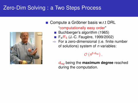
Zero-Dim Solving : a Two Steps Process

Compute a Gröbner basis w.r.t DRL“computationally easy order"Buchberger’s algorithm (1965)F4/F5 (J.-C. Faugère, 1999/2002)

⇒ For a zero-dimensional (i.e. finite numberof solutions) system of n variables:

O(n3·dreg

),

dreg being the maximum degree reachedduring the computation.

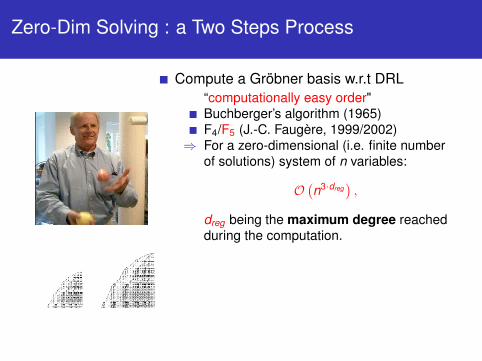
If #eq.= #var :dreg is gen. equal to n + 1.#Sol ≤

∏ni=1 degreeEqi (Bezout’s

bound)

Random Cases

For a semi-regular system of m (> n) quadratic equations overK[x1, . . . , xn] the degree of regularity is obtained from:

∑i≥0

aiz i =(1− z2)m

(1− z)n .

Random Cases


∑i≥0

aiz i =(1− z2)m

(1− z)n .

Example (3 variables and 5 equations)

1 + 3 · x + x2 − 5 · x3 − 5 · x4 + x5 + 3 · x6 + x7 + · · ·

Random Cases

For a semi-regular system of m (> n) quadratic equations overK[x1, . . . , xn] the degree of regularity is obtained from:∑

i≥0

aiz i =(1− z2)m

(1− z)n .

M. Bardet, J-C. Faugère, B. Salvyand B-Y. Yang.Asymptotic Behaviour of the Degreeof Regularity of Semi-RegularPolynomial Systems.MEGA 2005.

If m = n + 1,dreg ∼n→∞

⌈(n+1)

2

⌉.

Random Cases


∑i≥0

aiz i =(1− z2)m

(1− z)n .

If m = n + 1 :

dreg =

⌈(n + 1)

2

⌉.

A. Szanto.Multivariate Subresultants usingJouanolou’s Resultant Matrices.Journal of Pure and Applied Algebra.

Plan


2 MinRank


The MinRank problem

J.O. Shallit, G.S. Frandsen, and J.F. Buss.“The Computational Complexity of some Problems ofLinear Algebra". BRICS series report, 1996.

MR0

Input: R a commutative ring, n, k ∈ N·,M ∈Mn×n(R ∪ {x1, . . . , xk}),and a target rank r ∈ N·.Question: decide if there exists (λ1, . . . , λk ) ∈ Rk such that:

Rank(M(λ1, . . . , λk )

)≤ r .

Theorem (SFB’96)

MR0 is NP-Complete if R is a finite field.

The MinRank problem

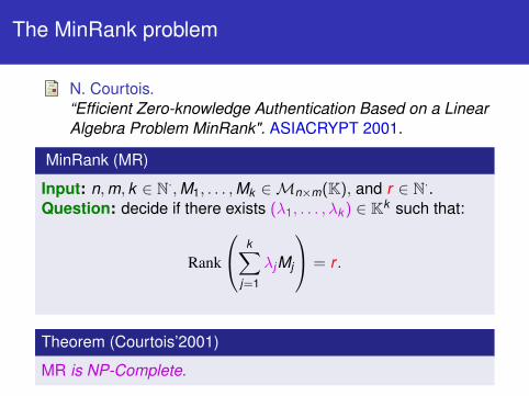
N. Courtois.“Efficient Zero-knowledge Authentication Based on a LinearAlgebra Problem MinRank". ASIACRYPT 2001.

MinRank (MR)

Input: n,m, k ∈ N·,M0, . . . ,Mk ∈Mn×m(K), and r ∈ N·.Question: decide if there exists (λ1, . . . , λk ) ∈ Kk such that:

Rank

k∑j=1

λjMj −M0

≤ r .

Theorem (Courtois’2001)

MR is NP-Complete.

The MinRank problem


MinRank (MR)

Input: n,m, k ∈ N·,M1, . . . ,Mk ∈Mn×m(K), and r ∈ N·.Question: decide if there exists (λ1, . . . , λk ) ∈ Kk such that:

Rank

k∑j=1

λjMj

= r .

Theorem (Courtois’2001)

MR is NP-Complete.

Applications of MinRank

Rank Decoding

A. V. Ourivski, T. Johansson.“New technique for decoding codes in the rank metricand its cryptography applications." Problems of Info.Transmission’2002

Matrix Rigidity

A. Kumar, S. V. Lokam, Vi. M. Patankar, J. Sarma.“Using Elimination Theory to construct Rigid Matrices".FSTTCS’09.

Applications of MinRank

Zero-Knowledge authentication protocol based on MR

N. Courtois.“Efficient Zero-knowledge Authentication Based on aLinear Algebra Problem MinRank". ASIACRYPT 2001.

Key Recovery on Multivariate Public Key Cryptosystems

A. Kipnis, A. Shamir.“Cryptanalysis of the HFE Public Key Cryptosystem byRelinearization". CRYPTO 99.

N. Courtois, L. Goubin.“Cryptanalysis of the TTM Cryptosystem".ASIACRYPT 2000.

L. Bettale, J.-C. Faugère, L. Perret.“Cryptanalysis of Multivariate and Odd-CharacteristicHFE Variants". PKC 2011

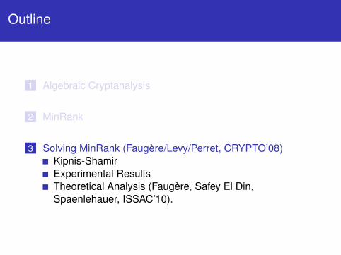
Outline


2 MinRank


Kipnis-Shamir’s Modeling – (I)

A. Kipnis and A. Shamir.“Cryptanalysis of the HFE Public Key Cryptosystem byRelinearization". CRYPTO 99.

Given n, k ∈ N·; M1, . . . ,Mk ∈Mn×n(K), and r ∈ N·.Find λ = (λ1, . . . , λk ) ∈ Kk such that:

Rk

k∑j=1

λjMj

= r .

Set Eλ =∑k

j=1 λjMj :

Rk(Eλ) = r ⇔ ∃(n−r) linearly indep. vectors X (i) ∈ Ker(Eλ).

We have(∑k

j=1 λjMj

)X (i) = 0n, for all i ,1 ≤ i ≤ n − r .

Kipnis-Shamir’s Modeling – (II)

Set Eλ =∑k

j=1 λjMj :

Rk(Eλ) = r ⇔ ∃(n−r) linearly indep. vectors X (i) ∈ Ker(Eλ).

Let X (i) = (x (i)1 , . . . , x (i)

n ), where x (i)j s are variables. Then :

k∑j=1

yjMj

x (1)1 · · · x (n−r)

1x (1)

2 · · · x (n−r)2

......

...x (1)

n · · · x (n−r)n

=

0 · · · 00 · · · 0...

......

0 · · · 0

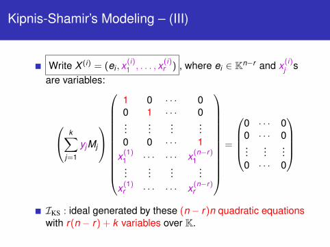
Kipnis-Shamir’s Modeling – (III)

Write X (i) = (ei , x(i)1 , . . . , x (i)

r ) , where ei ∈ Kn−r and x (i)j s

are variables:

k∑j=1

yjMj

1 0 · · · 00 1 · · · 0...

......

...0 0 · · · 1

x (1)1 · · · · · · x (n−r)

1...

......

...x (1)

r · · · · · · x (n−r)r

=

0 · · · 00 · · · 0...

......

0 · · · 0

IKS : ideal generated by these (n− r)n quadratic equationswith r(n − r) + k variables over K.

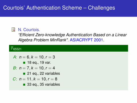
Courtois’ Authentication Scheme – Challenges


F65521

A: n = 6, k = 10, r = 318 eq., 19 var.

B: n = 7, k = 10, r = 421 eq., 22 variables

C: n = 11, k = 10, r = 833 eq., 35 variables

Courtois’ Authentication Scheme – Challenges


F65521

A: n = 6, k = 10, r = 3⇒ n = 6, k = 9, r = 318 eq., 19 var. ⇒ 18 eq., 18 var.

B: n = 7, k = 10, r = 4⇒ n = 7, k = 9, r = 421 eq., 22 variables⇒ 21 eq., 21 var.

C: n = 11, k = 10, r = 8⇒ n = 11, k = 9, r = 834 eq., 35 variables⇒ 34 eq., 34 var.

Experimental results with FGb (2008)

K = F65521

n k r TFGb Mem NFGb [Cou]

A 6 9 3 1 min. 400 Mb. 230.5 2106

B 7 9 4 1h45min. 3 Gb. 237.1 2122

8 9 5 91 h. 58.5 Gb. 243.4

C 11 9 8 264.4 2136

“not rigorous"

n k r dreg (theor.) dreg (observed) Bezout #SolA 6 9 3 19 5 218 210

B 7 9 4 22 6 221 212

8 9 5 28 8 227 213

C 11 9 8 33 ? 234 ?

Efficient attack but no theoretical explanation !!

Multi-Homogeneous Structure

Homogeneous

f (x1, . . . , xn) homogeneous of degree d ⇒

∀α ∈ K, f (α · x1, . . . , α · xn) = αd f (x1, . . . , xn).

Definition

Let [X (0), . . . ,X (k)] be a partition of the variables.f ∈ K[X (0), . . . ,X (k)] is multi-homogeneous of multi-degreed0, . . . ,dk if for all (α0, . . . , αk ) ∈ Kk+1:

f (α0 · X (0), . . . , αk · X (k)) = αd00 · · ·α

dkk f (X (0), . . . ,X (k)).

Multi-Homogeneous Structure

Property

The ideal IKS is multi-homogeneous ([Y ,X (1), . . . ,X (n−r)]).new bounds for the degree of regularitymulti-homogeneous Bézout bound

k∑j=1

yjMj

1 0 · · · 00 1 · · · 0...

......

...0 0 · · · 1

x (1)1 · · · · · · x (n−r)

1...

......

...x (1)

r · · · · · · x (n−r)r

=

0 · · · 00 · · · 0...

......

0 · · · 0

Theoretical Complexity

Conjecture

Let r ′ = n − r be a constant. We consider instances of MR withparameters

(n, k = r ′2, r = n − r ′

). For those particular

instances, we can compute the variety of IKS using Gröbnerbases in :

O(

ln (#K) n3 r ′2),

The complexity of our attack is polynomial for instances ofMinRank with

(n, k = r ′2, r = n − r ′

).

(n, k , r) A = (6,9,3) B = (7,9,4) C = (11,9,8)#Sol (MH Bézout bound) 213 215 222

Experimental #Sol 210 212

Complexity bound 238.9 246.2 266.3

Experimental Bound 230.5 237.1 264.3


J.-C. Faugère, M. Safey El Din, P.-J. Spaenlehauer.“Computing Loci of Rank Defects of Linear Matrices usingGrbner Bases and Applications to Cryptology.". ISSAC2009.

Theorem (Faugère, Safey El Din, Spaenlehauer)

Let (n, r , k) be the parameters of a MinRank instance, A = [ai,j ]

be the (r × r)-matrix with ai,j(t) =∑n−max(i,j)

`=0

(n−i`

)(n−j`

)t`. The

degree of regularity is ≤ 1 + deg (HS(t)) where HS(t) is thepolynomial obtained from the first positive terms of the series

(1− t)(n−r)2−k det A(t)

t(r2)

.


L. Bettale, J.-C. Faugère, L. Perret.“Cryptanalysis of Multivariate and Odd-Characteristic HFEVariants". PKC 2011

Main Results

Improved key recovery attack on HFEExtension of the attack to Multi-HFEPractical challenges brokenProved theoretical complexity of the attackCharacterization of equivalent keysAttack on Multi-HFE variants.Careful recovery of the secret key

Conclusion

Formerly

Algebraic techniques = modeling the problem by algebraicequations + computing a Gröbner basis.

New trend

Theoretical complexity analysis to explain the behavior of theattack.

Systematic use of structured systems (algebraiccryptanalysis of code-based systems).

J.-C. Faugère, M. Safey El Din, P.-J. Spaenlehauer.“Gröbner Bases of Bihomogeneous Ideals generated byPolynomials of Bidegree (1,1): Algorithms and Complexity".JSC 2011.

gröbner bases techniques in cryptography · gröbner bases techniques in cryptography ludovic...

Documents