Recent Advances in Hyperspectral Signal and Image Processing, Transworld Research Network, Trivandrum, Kerala, 2006.   ISBN: 81‐7895‐218‐1, Editor Chein‐I Chang. 

Greedy Modular Eigenspace Method for Hyperspectral Image Classification

Yang‐Lang Chang   Department of Electrical Engineering                                                                                         

National Taipei University of Technology                                                                                     Taipei, Taiwan, ROC 

E-mail: ylchang@ntut.edu.tw

The greedy modular eigenspace (GME) was developed by grouping highly correlated

hyper-spectral bands into a smaller subset of band modular regardless of the original order in terms of

wavelengths. The GME has shown effective in hyperspectral feature extraction. It utilizes the inherent

separability of different classes in hyperspectral images to reduce dimensionality and further to

generate a unique GME feature. The GME makes use of the data correlation matrix to reorder spectral

bands from which a group of feature eigenspaces can be generated to reduce dimensionality. It can be

implemented as a feature extractor to generate a particular feature eigenspace for each of the material

classes present in hyperspectral data. It avoids the bias problems of transforming the information into

linear combinations of bands as does the traditional principal components analysis (PCA). Compared

to the conventional PCA, it not only significantly increases the accuracy of image classification but

also dramatically improves the eigen-decomposition computational complexity. Experimental results

demonstrate that the proposed GME feature extractor is very effective and can be used as an

alternative compared to other feature extraction algorithms.

INTRODUCTION

Due to recent advances in remote sensing instruments the number of spectral bands used in these

instruments to collect data has significantly increased. It covers an abundance of applications from

satellite imaging, monitoring systems to medical imaging and industrial product inspection. But this

improved spectral resolution also comes at a price, known as the curse of dimensionality (Bellman,

1961) [1]. The term has been given a great deal of attention by researchers in the statistic, database,

and data mining communities to describe the difficulties associated with the feasibility of distribution

estimation in high-dimensional datasets. Numerous techniques have been developed for feature

extraction to reduce dimensionality without loss of class separability. The most widely used approach

is the principal components analysis (PCA) which reorganizes the data coordinates in accordance with

data variances so that features are extracted based on the magnitudes of their corresponding

eigenvalues (Richards and Jia, 1999) [2]. Fisher discriminant analysis uses the between-class and

within-class variances to extract desired features and to reduce dimensionality (Duda and Hart, 1973)

[3]. Another well-known approaches is the orthogonal subspace projection (OSP) recently developed

by Harsanyi and Chang (1994) [4]. OSP projects all undesired pixels into a space orthogonal to the

space generated by the desired pixels to achieve dimensionality reduction.

Most of them focus on the estimation of statistics at full dimensionality to extract classification

features. For example, conventional PCA assumes the covariances of different classes are the same

and the potential differences between class covariances are not explored. In contrast, we propose a

novel greedy modular eigenspace (GME) method overcomes the dependency on global statistics,

while preserving the inherent separability of the different classes. It utilizes the separability of

different classes in hyperspectral images to reduce dimensionality and further to generate a unique

GME feature. Most classifiers seek only one set of features that discriminates all classes simulta-

neously. This not only requires a large number of features, but also increases the complexity of the

potential decision boundary. Our proposed method makes use of the GME to develop a GME-based

feature extraction for hyperspectral imagery. It’s developed for land cover classification based on

feature selection of the same scene collected from hyperspectral remote sensing images. It presents a

framework for feature extraction of hyperspectral remote sensing images, which consists of two

algorithms, referred to as the GME (Chang, 2003) [5] and feature scale uniformity transformation

(GME/FSUT) (Chang, 2004) [6]. The GME method is designed to extract features by a simple and

efficient GME feature module, while the FSUT is performed to fuse most correlated features from

different data sources. They present a framework for multisource fusions of remote sensing images.

The GME is a spectral-based technique that explores the correlation among bands. Reordering the

bands regardless of the original order in terms of wavelengths in high-dimensional datasets is an

important characteristic of GME. It performs a greedy iteration search algorithm which reorders the

correlation coefficients in the data correlation matrix row by row, and column by column to group

highly correlated bands as GME feature eigenspaces that can be further used for feature extractions.

Each ground cover type or material class has a distinct set of GME-generated feature eigenspaces. The

FSUT makes use of the GME feature extraction method which tends to equalize all the bands in a

subgroup with highly correlated variances to avoid a potential bias problem that may occur in

conventional PCA (Jia, 1999) [7]. This fast feature extraction algorithm is proposed to unify GME sets

of different classes. It takes advantage of the special characteristics of GME to concentrate GME sets

of different classes into the most common feature subspaces. A distance measure based on GME was

then applied to decompose the similarity for land cover classification purposes.

FIG. 1: Data flow diagram of the proposed GME/FSUT classification scheme.

The goal of our proposed method is to develop a GME-based feature extraction technique that

combines different datasets in such a way that new types of data products can be produced. In our

previous work (Chang, 2003) [5], the GME was developed by grouping highly correlated bands into a

small set of bands. After finding a GME set, a FSUT is next performed to unify the feature scales of

these GME. The GME/FSUT carries out a feature extraction for the GME of different classes. To

demonstrate the advantages of the proposed method, we compared several different configurations,

which were categorized by their use of different options and distance measures.

This article presents a novel feature extraction algorithm. The approach makes use of the statistical

properties of the abundant feature characteristics of hyperspectral datasets while taking advantage of

the GME feature extraction method (Chang, 2003) [5]. The performance of the propose method is

evaluated by MODIS/ASTER airborne simulator (MASTER) images for land cover classification

during the PacRim II campaign. Experimental results demonstrate that the proposed GME approach is

an effective method for feature extractions. The rest of this article is organized as follows. In Section 2,

the proposed GME/FSUT classifier is described in detail. In Section 3, a set of experiments is

conducted to demonstrate the feasibility and utility of the proposed approach. Finally, in Section 4,

several conclusions are presented.

METHODOLOGY

Referring to Fig. 1, there are four stages to implementing our proposed GME classification scheme.

1) A GME transformation algorithm is applied to achieve dimensionality reduction and feature

extraction. 2) The second stage is a FSUT, which constructs an identical GME set for the purposes of

the feature extraction and the feature selection. 3) The third stage is a threshold decomposition, which

normalizes the scales of different feature bands. Then, a distance decomposition, also known as a

similarity measure, is performed for the classification. 4) Finally, a classification process is performed

for the classification.

Greedy Modular Eigenspaces

PCA has become the mainstream algorithm to advance the progress of high-dimensional data

analysis in many fields such as noise-whitened, feature extraction, dimensionality reduction, data

compression and target discrimination (Chang et al., 2002 and 2003) [8, 9]. The goal of PCA is to find

the principal components with their directions along the maximum variances of a data matrix. Chang

et al., 2002, demonstrated a feature selection method that used a loading factors matrix

eigen-analysis-based prioritization and a divergence-based band decorrelation [8]. It fully exploited

the usefulness of eigen-analysis for feature extraction in high-dimensional data classification. The

conventional low-dimensional classification methods that used single-pixel-based similarity measures

such like Gaussian maximum likelihood don’t work well in high-dimensional classification (Tu et al.,

1998) [10]. Instead, the spectral correlation of pixel vectors for high-dimensional data sets can provide

richer features to improve the classification accuracy. In addition, Chang et al., 2001, showed that the

use of second-order statistics, such as PCA that utilizes covariance matrix, can improve hyperspectral

classification performance more efficiently [11]. In this article, we also apply the second-order

statistics to the proposed GME method to improve the classification accuracy.

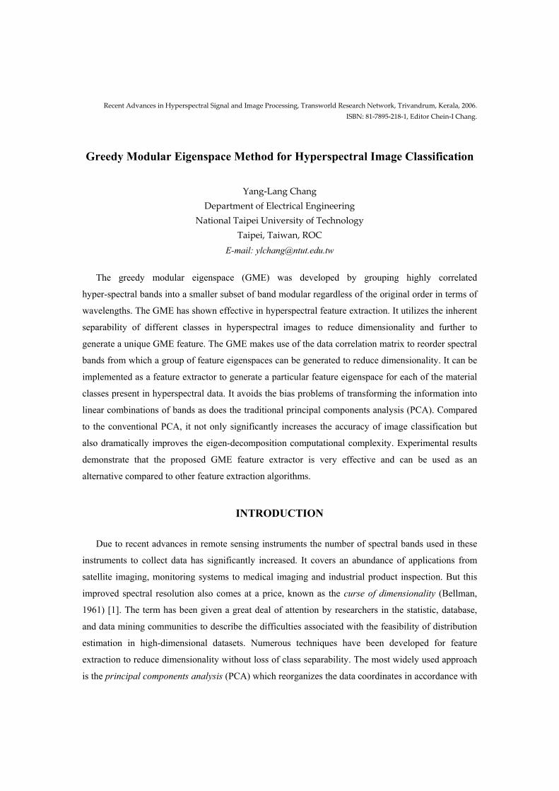
A visual scheme to display the magnitude of correlation matrix for emphasizing the second-order

statistics of high-dimensional data was proposed by Lee and Landgrebe, 1993 [12]. Shown in Fig. 2 is

a correlation matrix pseudo-color map (CMPM) in which the gray scale is used to represent the

magnitude of its corresponding correlation matrix. It is also equal to a modular subspace set Φk.

Different material classes have different value sequences of correlation matrices. It can be treated as

the special sequence codes for feature extractions. We define a correlation submatrix cΦkl(ml× ml)

which belongs to the lth

modular subspace Φkl of a complete set Φ

k and given by

Φk = ( Φk

1 , . . . Φkl , . . .Φ k

nk) (1)

for a class ωk, where ml and nk represent, respectively, the number of bands (feature spaces) in modular

subspace Φkl, and the total number of modular subspaces for a complete set Φ

k, i.e. l∈{1,...,nk} as

shown in Fig. 2. The original correlation matrix cX

k(mt×mt) is decomposed into

cXk(mt×mt) =cΦk1 (m1 ×m1),...cΦk

l (ml×ml),....cΦ k nk

(mnk×mnk

) (2)

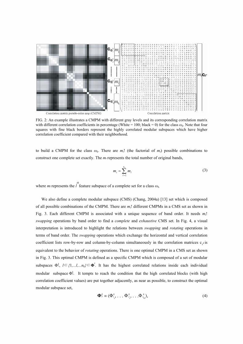
FIG. 2: An example illustrates a CMPM with different gray levels and its corresponding correlation matrix with different correlation coefficients in percentage (White = 100; black = 0) for the class ωk. Note that four squares with fine black borders represent the highly correlated modular subspaces which have higher correlation coefficient compared with their neighborhood.

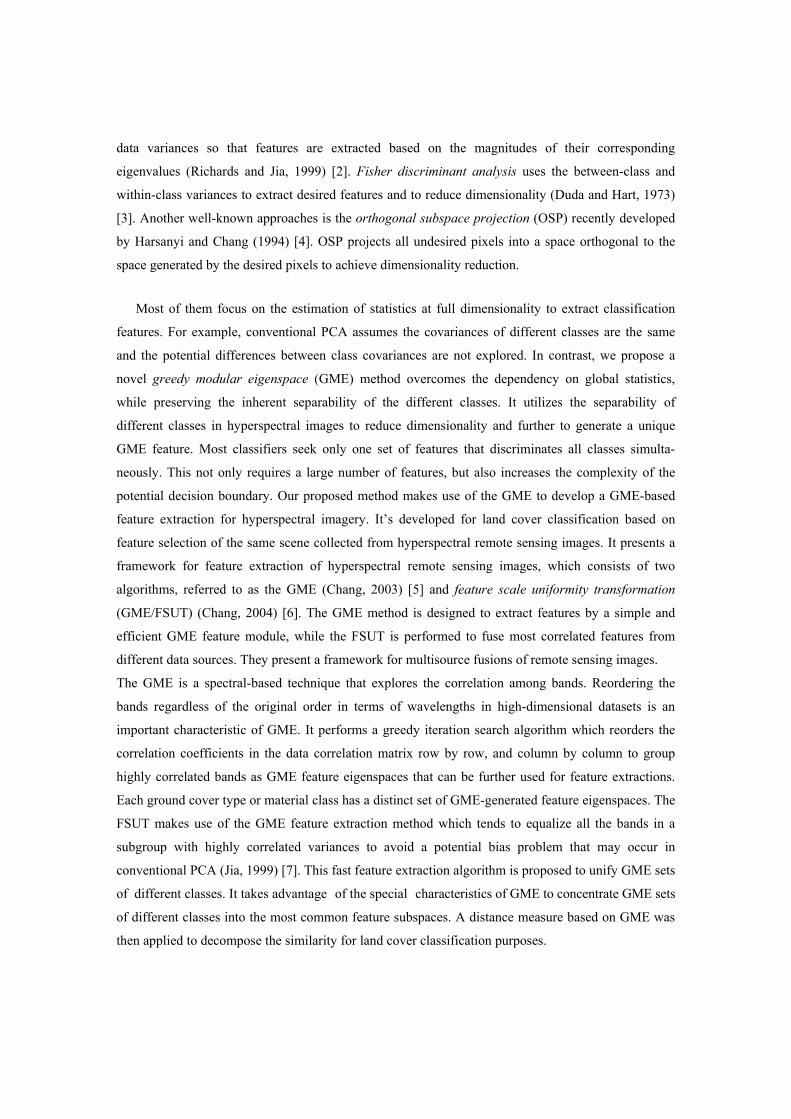
to build a CMPM for the class ωk. There are mt! (the factorial of mt) possible combinations to

construct one complete set exactly. The mt represents the total number of original bands,

∑=

=kn

llt mm

1 (3)

where ml represents the lth

feature subspace of a complete set for a class ωk.

We also define a complete modular subspace (CMS) (Chang, 2004a) [13] set which is composed

of all possible combinations of the CMPM. There are mt! different CMPMs in a CMS set as shown in

Fig. 3. Each different CMPM is associated with a unique sequence of band order. It needs mt!

swapping operations by band order to find a complete and exhaustive CMS set. In Fig. 4, a visual

interpretation is introduced to highlight the relations between swapping and rotating operations in

terms of band order. The swapping operations which exchange the horizontal and vertical correlation

coefficient lists row-by-row and column-by-column simultaneously in the correlation matrices cX

k is

equivalent to the behavior of rotating operations. There is one optimal CMPM in a CMS set as shown

in Fig. 3. This optimal CMPM is defined as a specific CMPM which is composed of a set of modular

subspaces Φkl , l∈{1,...l,...nk}∈Φ

k. It has the highest correlated relations inside each individual

modular subspace Φkl. It tempts to reach the condition that the high correlated blocks (with high

correlation coefficient values) are put together adjacently, as near as possible, to construct the optimal

modular subspace set,

Φko = (Φ k

1o, . . . Φ k

2o, . . .Φ k

nko), (4)

FIG. 3: (a.) The initial CMPM for four original bands (A, B, C and D), mt= 4, is applied to the exhaustive swapping operations by band order. Each corresponding correlation has different correlation coefficient in percentage as indicated in each box. (b.) An example shows a CMS set which is composed of 24 (mt! = 4!) possible CMPMs. The CMPM with a dotted-line square is the optimal CMPM in a CMS set.

in the diagonal of CMPM. It is too expensive to make an exhaustive computation for a large amount

of mt to find an optimal CMPM in a CMS set. In order to overcome this drawback, we develop a fast

searching algorithm, called greedy modular subspaces transformation (GMET), based on the fact that

highly correlated bands often appear adjacently to each other for remote sensing high-dimensional

data sets (Richards and Jia, 1999) [2] to construct an alternative greedy CMPM (modular subspace)

instead of the optimal CMPM. This new defined greedy CMPM can be also treated as a GME feature

module set Φk, which uses the same notation as the complete set Φ

k defined in Eq. (1). It can not only

reduce the redundant operations in finding the greedy CMPM but also provides an efficient method to

construct GME sets which have suitable properties for feature extractions of high-dimensional data

sets.

In this algorithm, every positive correlation coefficient ci,j, which is an absolute value, is compared

with a correlation coefficient threshold value 0 ≤ tc≤ 1 by band order adjacently. A greedy searching

iteration is initially carried out at c0,0∈cX

k(mt×mt) as a new seed to build a GME set. All attributes of

cXk (mt×mt) are first set as available except c0,0. The proposed GMET is stated as follows.

FIG. 4: The rotation operation between the Block K and Block 2 is performed by swapping their horizontal and vertical correlation coefficient lists row-by-row and column-by-column. Note that a pair of blocks (squares) switched by this swapping operation in terms of band order should have the same size of any length along the diagonal of correlation matrices. The Fixed Blk 1 and Fixed Blk 2 will rotate 90 degrees at the same locations.

Step 1. Initialization: A new modular eigenspace Φkl∈Φ

k for a class ωk is initialized by a new

correlation coefficient cd,d, where cd,d and d are defined as the first available element and its

subindex in the diagonal list [c0,0,...cmt-1, mt-1] of the correlation matrix cX

k respectively. This

diagonal coefficient cd,d is set to used and then assigned as the current ci,j, i.e. the only one

activated at the current time. Then, go to step 2. Note that this GMET algorithm is terminated

if the last diagonal coefficient cd,d is already set to used and the last subgroup Φ k nk

of the GME

has been obtained for class ωk.

Step 2. If the column subindex j of the current ci,j has reached the last column (i.e. j = mt−1) in the

correlation matrix, then a new modular eigenspace Φkl is constructed with all used correlation

coefficients ∈Φkl, these used coefficients are then removed from the correlation matrix, and

the algorithm goes to step 1 for another round to find a new modular eigenspace. Otherwise, it

goes to step 3.

Step 3. GMET moves the current ci,j to the next adjacent column ci,j +1 which will act as the current ci,j,

i.e. ci,j→ci,j +1. If the current ci,j is available and its value is larger than tc, then go to step 4.

Otherwise, go to step 2.

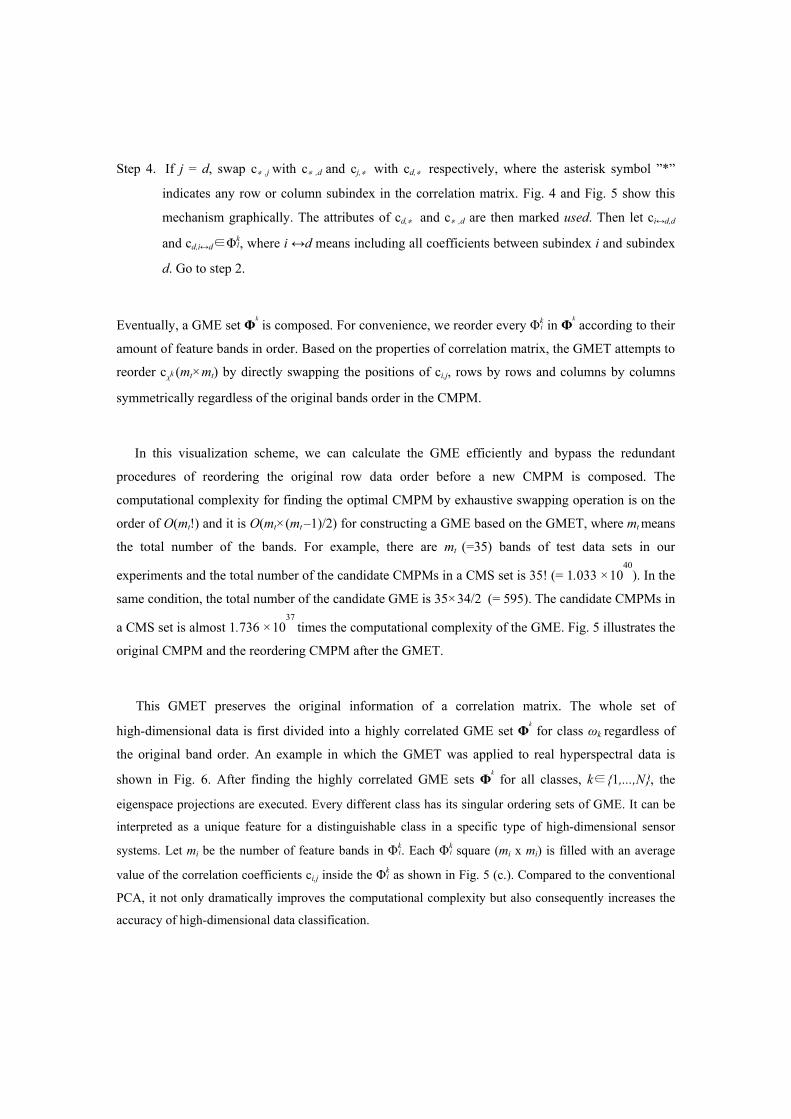
Step 4. If j = d, swap c∗ ,j with c∗ ,d and cj,∗ with cd,∗ respectively, where the asterisk symbol ”*”

indicates any row or column subindex in the correlation matrix. Fig. 4 and Fig. 5 show this

mechanism graphically. The attributes of cd,∗ and c∗ ,d are then marked used. Then let ci↔d,d

and cd,i↔d∈Φkl, where i ↔d means including all coefficients between subindex i and subindex

d. Go to step 2.

Eventually, a GME set Φk is composed. For convenience, we reorder every Φk

i in Φk according to their

amount of feature bands in order. Based on the properties of correlation matrix, the GMET attempts to

reorder cX

k (mt×mt) by directly swapping the positions of ci,j, rows by rows and columns by columns

symmetrically regardless of the original bands order in the CMPM.

In this visualization scheme, we can calculate the GME efficiently and bypass the redundant

procedures of reordering the original row data order before a new CMPM is composed. The

computational complexity for finding the optimal CMPM by exhaustive swapping operation is on the

order of O(mt!) and it is O(mt×(mt –1)/2) for constructing a GME based on the GMET, where mt means

the total number of the bands. For example, there are mt (=35) bands of test data sets in our

experiments and the total number of the candidate CMPMs in a CMS set is 35! (= 1.033 ×1040

). In the

same condition, the total number of the candidate GME is 35×34/2 (= 595). The candidate CMPMs in

a CMS set is almost 1.736 ×1037

times the computational complexity of the GME. Fig. 5 illustrates the

original CMPM and the reordering CMPM after the GMET.

This GMET preserves the original information of a correlation matrix. The whole set of

high-dimensional data is first divided into a highly correlated GME set Φk for class ωk regardless of

the original band order. An example in which the GMET was applied to real hyperspectral data is

shown in Fig. 6. After finding the highly correlated GME sets Φk for all classes, k∈{1,...,N}, the

eigenspace projections are executed. Every different class has its singular ordering sets of GME. It can be

interpreted as a unique feature for a distinguishable class in a specific type of high-dimensional sensor

systems. Let mi be the number of feature bands in Φki. Each Φk

i square (mi x mi) is filled with an average

value of the correlation coefficients ci,j inside the Φki as shown in Fig. 5 (c.). Compared to the conventional

PCA, it not only dramatically improves the computational complexity but also consequently increases the

accuracy of high-dimensional data classification.

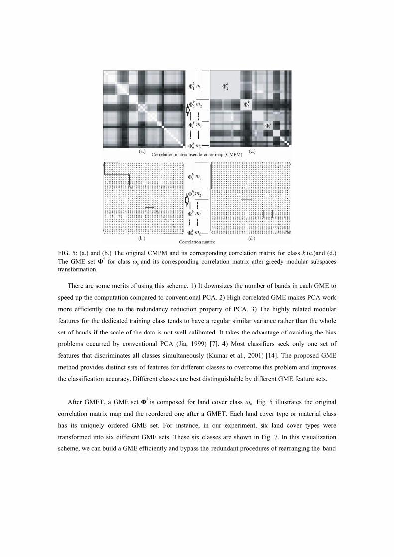
FIG. 5: (a.) and (b.) The original CMPM and its corresponding correlation matrix for class k.(c.)and (d.) The GME set Φ

k for class ωk and its corresponding correlation matrix after greedy modular subspaces

transformation.

There are some merits of using this scheme. 1) It downsizes the number of bands in each GME to

speed up the computation compared to conventional PCA. 2) High correlated GME makes PCA work

more efficiently due to the redundancy reduction property of PCA. 3) The highly related modular

features for the dedicated training class tends to have a regular similar variance rather than the whole

set of bands if the scale of the data is not well calibrated. It takes the advantage of avoiding the bias

problems occurred by conventional PCA (Jia, 1999) [7]. 4) Most classifiers seek only one set of

features that discriminates all classes simultaneously (Kumar et al., 2001) [14]. The proposed GME

method provides distinct sets of features for different classes to overcome this problem and improves

the classification accuracy. Different classes are best distinguishable by different GME feature sets.

After GMET, a GME set Φk is composed for land cover class ωk. Fig. 5 illustrates the original

correlation matrix map and the reordered one after a GMET. Each land cover type or material class

has its uniquely ordered GME set. For instance, in our experiment, six land cover types were

transformed into six different GME sets. These six classes are shown in Fig. 7. In this visualization

scheme, we can build a GME efficiently and bypass the redundant procedures of rearranging the band

FIG. 6: The GME sets for different ground cover classes ωk,...ωj. A GME set Φk is composed of a group of

modular eigenspaces ( Φk1 , . . . Φk

l , . . .Φ k nk

).

order from the original high-dimensional datasets. Moreover, the GMET algorithm can tremendously

reduce the eigen-decomposition computation compared to conventional PCA feature extraction. The

computational complexity for conventional PCA is of the order of O (mt x mt) and it is O(Σ nk

i=1 m2i) for

GME (Jia, 1999) [7]. The GME preserves the original information of a correlation matrix.

Feature Scale Uniformity Transformation

After fining GME sets Φk, a fast and effective GME/FSUT is performed to unify the feature scales

of these GME sets to an identical GME set ΦI. We uses intersection (AND) operations (Chang, 2004)

[6] applied to the band numbers inside each GME module ωk to unify the feature scales of different

classes produced by GMET and construct an identical intersection GME (IGME) ΦI set for all classes

ωk, k∈{1,...,N}. A concept block diagram of GME is shown in Fig. 8. Every different class has the

same IGME set ΦI after the GME.

The GME/FSUT performing a searching iteration to build an identical IGME set ΦI is initially

carried out on a newly formed IGME feature module ΦIl, where l∈{1,...,n}and ΦIl

∈ΦI, in which the

first band bi, where i∈{1,...,n} and i = 1, of the largest GME module Φ11 is chosen to form a IGME set

ΦI. Each band bi is assigned an attribute during a GME/FSUT. If the attribute of bi is set as available,

it means this bi has not been yet assigned to any identical IGME set ΦI. If a bi is assigned to a ΦI, the

attribute of this bi is set to used. All attributes of the original bi, i∈{1,...,n}, are first set as available.

FIG. 7: GME sets for the six ground cover types used in the experiment. Each of them can be treated as a unique feature for a distinguishable class.

The GME/FSUT was applied to three land cover types used in our experiment as shown in Fig. 9. The

proposed GME/FSUT algorithm is as follows:

Step 1. Initialization: a new IGME feature module ΦIl, where ΦIl

∈ΦI, is initialized by a new

band bi inside a GME module Φk1 , where bi is defined as the first available band and

Φk1 as the largest GME module of the class ωk. This new band bi is assigned to the

newly created IGME feature module ΦIl and is then set as the current bi, i.e. the only

one activated at the current time. Then, go to step 2. Note that this GME/FSUT

algorithm is terminated if the last band bi is already set to used and the final IGME

feature module ΦIl, ΦIl

∈ΦI, has been obtained.

Step 2. If the current band bi and all its related bands have all been set to used, then a IGME

feature module ΦIl is constructed with all used bands, these used bands are removed

from the band list, and the GME/FSUT algorithm goes to step 1 for another round to

find a new IGME feature module ΦIl. Otherwise, it goes to step 3.

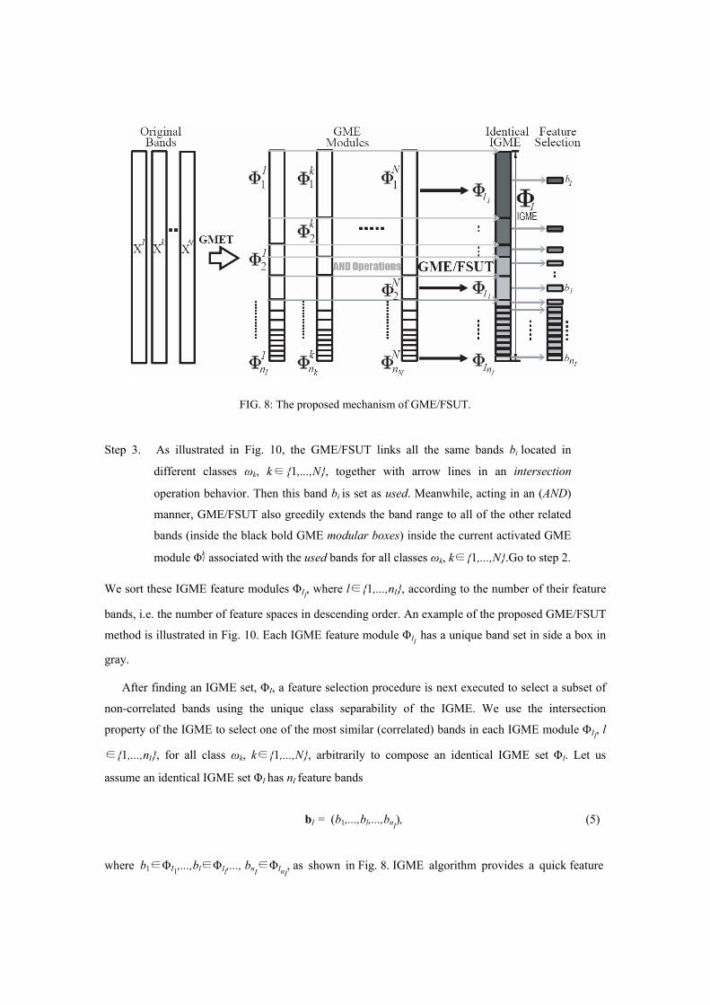
FIG. 8: The proposed mechanism of GME/FSUT.

Step 3. As illustrated in Fig. 10, the GME/FSUT links all the same bands bi located in

different classes ωk, k∈{1,...,N}, together with arrow lines in an intersection

operation behavior. Then this band bi is set as used. Meanwhile, acting in an (AND)

manner, GME/FSUT also greedily extends the band range to all of the other related

bands (inside the black bold GME modular boxes) inside the current activated GME

module Φkl associated with the used bands for all classes ωk, k∈{1,...,N}.Go to step 2.

We sort these IGME feature modules ΦIl, where l∈{1,...,nI}, according to the number of their feature

bands, i.e. the number of feature spaces in descending order. An example of the proposed GME/FSUT

method is illustrated in Fig. 10. Each IGME feature module ΦIl has a unique band set in side a box in

gray.

After finding an IGME set, ΦI, a feature selection procedure is next executed to select a subset of

non-correlated bands using the unique class separability of the IGME. We use the intersection

property of the IGME to select one of the most similar (correlated) bands in each IGME module ΦIl, l

∈{1,...,nI}, for all class ωk, k∈{1,...,N}, arbitrarily to compose an identical IGME set ΦI. Let us

assume an identical IGME set ΦI has nI feature bands

bI = (b1,...,bl,...,bnI), (5)

where b1∈ΦI1,...,bl∈ΦIl,..., bnI

∈ΦInI, as shown in Fig. 8. IGME algorithm provides a quick feature

FIG. 9: GME sets for the three land cover types used in the experiment. The squares on the left are the original CMPM. The CMPM on the right are the reordered ones after a GMET. The GME feature modules (Φk

1,...Φkl,...Φ k

nk) of different GME sets Φ

k are illustrated as the modular boxes in the middle column.

selection procedure of the most significant features and an instant distance measure of the

hyperspectral samples compared to the conventional feature extraction methods.

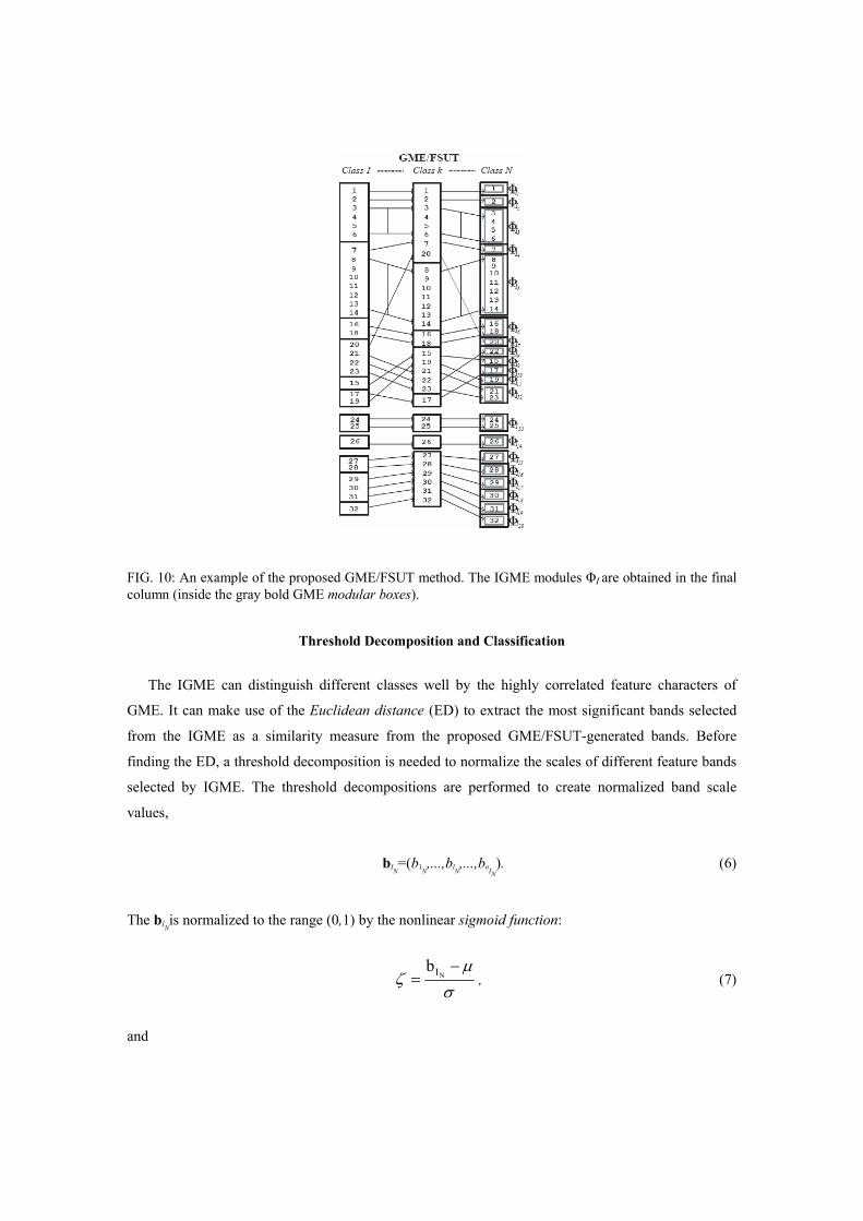
FIG. 10: An example of the proposed GME/FSUT method. The IGME modules ΦI are obtained in the final column (inside the gray bold GME modular boxes).

Threshold Decomposition and Classification

The IGME can distinguish different classes well by the highly correlated feature characters of

GME. It can make use of the Euclidean distance (ED) to extract the most significant bands selected

from the IGME as a similarity measure from the proposed GME/FSUT-generated bands. Before

finding the ED, a threshold decomposition is needed to normalize the scales of different feature bands

selected by IGME. The threshold decompositions are performed to create normalized band scale

values,

bIN=(b1N

,...,blN,...,bnIN

). (6)

The bINis normalized to the range (0,1) by the nonlinear sigmoid function:

σμ

ζ−

= NIb, (7)

and

)exp(11)(b

NI ζζ

t−+= , (8)

where µ, σ and t denote the mean and the standard deviation of the normalized band scale values bIN

and a threshold value respectively. This new normalized scale values bINare converted into binary

values. We also define normalized binary values of ED,

eIN=( e 1

IN ,..., e k

IN ,..., eN

IN), (9)

for all classes ωk, k∈{1,...,N}. The threshold decomposition function T(·) then transforms the

normalized scale values bIN into the binary values ED eIN

for all classes ωk.

After the normalization, the ED eIN is then decomposed for the purpose of distance measure. Note

that only one band for each IGME feature module ΦIl, l∈{1,...,nI}, is selected to decompose the ED eIN

,

as shown in Fig. 8. A normalized ED eIN function E(·) of an identical IGME set with nI feature bands is

defined as:

∑=

=In

iixx

1

2I

~)(eN

, (10)

where x~

= x - x—

is the mean-normalized vector of sample x. The sample x is equal to bIN for the

training samples. Here, eIN(x) represents the distance between the query test samples X and the mean

vector of training samples based on the IGME feature module ΦIl. This distance decomposition is

applied to all classes ωk to generate an identical normalized ED eIN. After finding the normalized ED

eIN from the previous stage, a minimum distance classification is next performed. By comparing the

normalized ED eIN between training samples and test samples, it is easy to identify the correct classes

to which the test samples belong. The training samples x are first applied to the GME/FSUT to

construct the IGME feature module ΦIl. The final determined classes are then induced by applying the

test samples X to the GME/FSUT stage for feature extractions and minimum distance classifications.

FIG. 11: The map of the Au-Ku test site used in the experiment.

EXPERIMENTAL RESULTS

A plantation area in Au-Ku on the east coast of Taiwan as shown in Fig. 11 was chosen for

investigation. The image data was obtained by the MASTER as part of the PacRim II project (Hook et

al., 2000) [15]. A ground survey was made of the selected six land cover types at the same time. The

proposed GME method was applied to 35 bands selected from the 50 contiguous bands (excluding the

low signal-to-noise ratio mid-infrared channels) (Hook et al., 2000) [15] of MASTER. Six land cover

classes, sugar cane A, sugar cane B, seawater, pond, bare soil and rice are used in the experiment. The

criterion for calculating the classification accuracy of experiments was based on exhaustive test cases.

One hundred and fifty labeled samples were randomly collected from ground survey datasets by

iterating every fifth sample interval for each class. Thirty labeled samples were chosen as training

samples, while the rest were used as test samples, i.e. the samples were partitioned into 30 (20%)

training and 120 (80%) test samples for each test case. Three correlation coefficient threshold values,

tc=0.75, 0.80 and 0.85, were selected to carry out GMET. Finally, the accuracy was obtained by

averaging all of the multiple combinations stated above.

We compared several different configurations. Two main groups are compared in Fig. 12. The first

group is for GME (the bolder lines in gray). In this case, the GME was applied to MASTER datasets

to generate the IGME. One band was arbitrarily selected for each IGME feature module ΦkIl , l∈

{1,...,nI}, to decompose the normalized ED and apply to minimum distance classifier. For the second

group, the same datasets were used as for the first group, thus they was used to make a comparison

between the conventional Euclidean distance and our proposed GME methods. The Euclidean upper

bound, Euclidean average bands and Euclidean lower bound represent respectively the best upper bound feature bands, the average bands (between upper bound and lower bound) and the worst

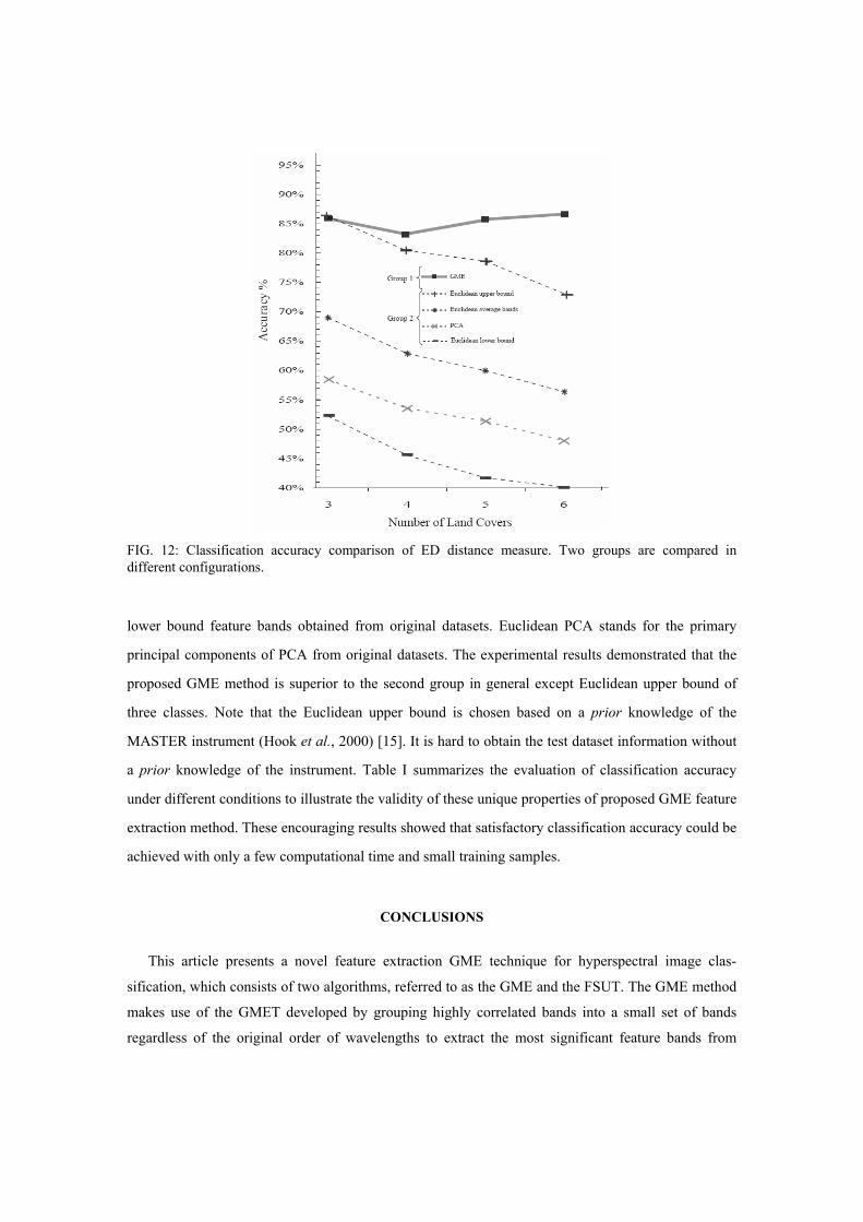
FIG. 12: Classification accuracy comparison of ED distance measure. Two groups are compared in different configurations.

lower bound feature bands obtained from original datasets. Euclidean PCA stands for the primary

principal components of PCA from original datasets. The experimental results demonstrated that the

proposed GME method is superior to the second group in general except Euclidean upper bound of

three classes. Note that the Euclidean upper bound is chosen based on a prior knowledge of the

MASTER instrument (Hook et al., 2000) [15]. It is hard to obtain the test dataset information without

a prior knowledge of the instrument. Table I summarizes the evaluation of classification accuracy

under different conditions to illustrate the validity of these unique properties of proposed GME feature

extraction method. These encouraging results showed that satisfactory classification accuracy could be

achieved with only a few computational time and small training samples.

CONCLUSIONS

This article presents a novel feature extraction GME technique for hyperspectral image clas-

sification, which consists of two algorithms, referred to as the GME and the FSUT. The GME method

makes use of the GMET developed by grouping highly correlated bands into a small set of bands

regardless of the original order of wavelengths to extract the most significant feature bands from

high-dimensional datasets, while the FSUT is performed to uniformity most correlated feature scales

from different data sources. The proposed GME algorithm is efficient with little computational

complexity. It uses intersection (AND) operations applied to the band numbers inside each GME

module to unify the feature scales of GME and construct an identical IGME feature module set. It can

be implemented as a band selector to generate a particular feature band set for each material class.

The experimental results demonstrated that the feature bands selected from the MASTER datasets

by the GME algorithm contain discriminatory properties crucial to subsequent classification.

TABLE I: Summary evaluation of classification accuracy for different feature extraction methods and number of classes.

Moreover, compared to conventional feature extraction techniques, the IGME feature modules have

very good abilities to adapt to the minimum distance classifiers. They make use of the potential

significant separability of GME to select a unique set of most important feature bands in

high-dimensional datasets. The proposed GME/FSUT algorithm provides a fast way to find the most

significant feature bands and to speed up the distance decomposition compared to GME features.

ACKNOWLEDGMENTS

This work was supported by the National Science Council, Taiwan, under Grant No. NSC

94-2212-E027-024.

REFERENCES

[1] R. E. Bellman, Adaptive Control Processes: A Guided Tour, Princeton University Press, New Jersey, NJ, 1961.

[2] J. A. Richards and X. Jia, Remote Sensing Digital Image Analysis, An Introduction, 3rd ed., Springer-

Verlag, New York, 1999. [3] R. Duda and P. Hart, Pattern Classification and Scene Analysis, John Wiley & Sons, New York, 1973. [4] J. Harsanyi and C.-I. Chang, “Hyperspectral image classification and dimensionality reduction: an

orthogonal subspace projection approach,” IEEE Trans. Geosci. Remote Sensing 32, no. 4, pp. 779– 785, 1994.

[5] Y. L. Chang, C. C. Han, K. C. Fan, K. S. Chen, C. T. Chen, and J. H. Chang, “Greedy modular

eigenspaces and positive Boolean function for supervised hyperspectral image classification,” Optical Engineering 42, no. 9, pp. 2576–2587, 2003.

[6] Y. L. Chang, C. C. Han, H. Ren, C.-T. Chen, K. S. Chen, and K. C. Fan, “Data fusion of hyperspectral

and SAR images,” Optical Engineering 43, no. 8, pp. 1787–1797, 2004. [7] X. Jia and J. A. Richards, “Segmented principal components transformation for efficient hyperspectral

remote-sensing image display and classification,” IEEE Trans. Geosci. Remote Sensing 37, no. 1, pp. 538–542, 1999.

[8] C.-I. Chang, Q. Du, T. L. Sun, and M. L. G. Althouse, “A joint band prioritization and band decorre-

lation approach to band selection for hyperspectral image classification,” IEEE Trans. Geosci. Remote Sensing 37, no. 6, pp. 2631–2641, 1999.

[9] C.-I. Chang and Q. Du, “Interference and noise adjusted principal components analysis,” IEEE Trans.

Geosci. Remote Sensing 37, no. 5, pp. 2387–2396, 1999. [10] T. Tu, C.-H. Chen, J.-L. Wu, and C.-I. Chang, “A fast two-stage classification method for high

dimensional remote sensing data,” IEEE Trans. Geosci. Remote Sensing 36, no. 5, pp. 182–191, 1998. [11] C.-I. Chang and S.-S. Chiang, “Discrimination measures for target classification,” in Geoscience and

Remote Sensing Symposium, IGARSS’01, IEEE International 4, pp. 1871–1873, 2001. [12] C. Lee and D. A. Landgrebe, “Analyzing high-dimensional multispectral data,” IEEE Trans. Geosci.

Remote Sensing 31, no. 4, pp. 792–800, 1993. [13] Y. L. Chang, C. C. Han, H. Ren, F. D. Jou, K. C. Fan, and K. S. Chen, “A modular eigen subspace

scheme for high-dimensional data classification,” Future Generation Computer Systems 20, no. 7, pp. 1131–1143, 2004.

[14] J. G. S. Kumar and M. M. Crawford, “Best-bases feature extraction algorithms for classification of

hyperspectral data,” IEEE Trans. Geosci. Remote Sensing 39, no. 7, pp. 1368–1379, 2001. [15] S. J. Hook, J. J. Myers, K. J. Thome, M. Fitzgerald, and A. B. Kahle, “The MODIS/ASTER airborne

simulator (MASTER) -a new instrument for earth science studies,” Remote Sensing of Environment 76, Issue 1, pp. 93–102, 2000.