(green energy and technology) kun sang lee (auth.)-underground thermal energy...

Green Energy and Technology

For further volumes:http://www.springer.com/series/8059

http://www.springer.com/series/8059

Kun Sang Lee

Underground ThermalEnergy Storage

123

Kun Sang LeeDepartment of Natural Resources

and Environmental EngineeringHanyang UniversitySeoulSouth Korea

ISSN 1865-3529 ISSN 1865-3537 (electronic)ISBN 978-1-4471-4272-0 ISBN 978-1-4471-4273-7 (eBook)DOI 10.1007/978-1-4471-4273-7Springer London Heidelberg New York Dordrecht

Library of Congress Control Number: 2012942260

� Springer-Verlag London 2013

Whilst we have made considerable efforts to contact all holders of copyright material contained in thisbook. We have failed to locate some of them. Should holders wish to contact the Publisher, we willmake every effort to come to some arrangement with them.

This work is subject to copyright. All rights are reserved by the Publisher, whether the whole or part ofthe material is concerned, specifically the rights of translation, reprinting, reuse of illustrations,recitation, broadcasting, reproduction on microfilms or in any other physical way, and transmission orinformation storage and retrieval, electronic adaptation, computer software, or by similar or dissimilarmethodology now known or hereafter developed. Exempted from this legal reservation are briefexcerpts in connection with reviews or scholarly analysis or material supplied specifically for thepurpose of being entered and executed on a computer system, for exclusive use by the purchaser of thework. Duplication of this publication or parts thereof is permitted only under the provisions ofthe Copyright Law of the Publisher’s location, in its current version, and permission for use must alwaysbe obtained from Springer. Permissions for use may be obtained through RightsLink at the CopyrightClearance Center. Violations are liable to prosecution under the respective Copyright Law.The use of general descriptive names, registered names, trademarks, service marks, etc. in thispublication does not imply, even in the absence of a specific statement, that such names are exemptfrom the relevant protective laws and regulations and therefore free for general use.While the advice and information in this book are believed to be true and accurate at the date ofpublication, neither the authors nor the editors nor the publisher can accept any legal responsibility forany errors or omissions that may be made. The publisher makes no warranty, express or implied, withrespect to the material contained herein.

Printed on acid-free paper

Springer is part of Springer Science+Business Media (www.springer.com)

Contents

1 Introduction . . . . . . . . . . . . . . . . . . . . . . . . . . . . . . . . . . . . . . . . 11.1 Energy Storage . . . . . . . . . . . . . . . . . . . . . . . . . . . . . . . . . . . 1

1.1.1 Energy Demand. . . . . . . . . . . . . . . . . . . . . . . . . . . . . 11.1.2 Energy Storage Methods. . . . . . . . . . . . . . . . . . . . . . . 31.1.3 Energy Storage History . . . . . . . . . . . . . . . . . . . . . . . 41.1.4 Thermal Energy Storage . . . . . . . . . . . . . . . . . . . . . . . 51.1.5 Various Aspects of TES . . . . . . . . . . . . . . . . . . . . . . . 10

References . . . . . . . . . . . . . . . . . . . . . . . . . . . . . . . . . . . . . . . . . . 13

2 Underground Thermal Energy Storage . . . . . . . . . . . . . . . . . . . . . 152.1 Introduction . . . . . . . . . . . . . . . . . . . . . . . . . . . . . . . . . . . . . 15

2.1.1 Ground Temperature . . . . . . . . . . . . . . . . . . . . . . . . . 162.1.2 Historical Development . . . . . . . . . . . . . . . . . . . . . . . 172.1.3 Advantages . . . . . . . . . . . . . . . . . . . . . . . . . . . . . . . . 17

2.2 Classification . . . . . . . . . . . . . . . . . . . . . . . . . . . . . . . . . . . . 182.2.1 Storage Temperature . . . . . . . . . . . . . . . . . . . . . . . . . 182.2.2 Storage Technology . . . . . . . . . . . . . . . . . . . . . . . . . . 20

2.3 Characteristics of Underground Storage Systems . . . . . . . . . . . . 212.3.1 Efficiency Benefits . . . . . . . . . . . . . . . . . . . . . . . . . . 222.3.2 Availability . . . . . . . . . . . . . . . . . . . . . . . . . . . . . . . . 232.3.3 Potential Applications Sectors . . . . . . . . . . . . . . . . . . . 232.3.4 Temperature Levels . . . . . . . . . . . . . . . . . . . . . . . . . . 232.3.5 Humidity Aspects . . . . . . . . . . . . . . . . . . . . . . . . . . . 242.3.6 Load Coverage . . . . . . . . . . . . . . . . . . . . . . . . . . . . . 24

2.4 Advantages and Limitations of UndergroundStorage Systems . . . . . . . . . . . . . . . . . . . . . . . . . . . . . . . . . . 242.4.1 Advantages . . . . . . . . . . . . . . . . . . . . . . . . . . . . . . . . 252.4.2 Limitations . . . . . . . . . . . . . . . . . . . . . . . . . . . . . . . . 25

References . . . . . . . . . . . . . . . . . . . . . . . . . . . . . . . . . . . . . . . . . . 26

v

http://dx.doi.org/10.1007/978-1-4471-4273-7_1

http://dx.doi.org/10.1007/978-1-4471-4273-7_1

http://dx.doi.org/10.1007/978-1-4471-4273-7_1#Sec1












http://dx.doi.org/10.1007/978-1-4471-4273-7_1#Bib1

http://dx.doi.org/10.1007/978-1-4471-4273-7_2

http://dx.doi.org/10.1007/978-1-4471-4273-7_2





































3 Basic Theory and Ground Properties . . . . . . . . . . . . . . . . . . . . . . 273.1 Basic Physical Mechanism . . . . . . . . . . . . . . . . . . . . . . . . . . . 27

3.1.1 Hydrological Flow in the Aquifer . . . . . . . . . . . . . . . . 283.1.2 Hydrological Flow in Borehole . . . . . . . . . . . . . . . . . . 303.1.3 Heat Transfer Mechanism. . . . . . . . . . . . . . . . . . . . . . 30

3.2 Hydrogeological Conditions . . . . . . . . . . . . . . . . . . . . . . . . . . 373.2.1 Aquifer Systems . . . . . . . . . . . . . . . . . . . . . . . . . . . . 383.2.2 Borehole Systems . . . . . . . . . . . . . . . . . . . . . . . . . . . 40

3.3 Determination of Hydrogeological Properties . . . . . . . . . . . . . . 413.3.1 Step-Drawdown Tests . . . . . . . . . . . . . . . . . . . . . . . . 413.3.2 Well Flow Equations . . . . . . . . . . . . . . . . . . . . . . . . . 443.3.3 Anisotropy Test. . . . . . . . . . . . . . . . . . . . . . . . . . . . . 473.3.4 Dispersivity Testing . . . . . . . . . . . . . . . . . . . . . . . . . . 48

3.4 Determination of Thermal Properties . . . . . . . . . . . . . . . . . . . . 503.4.1 Development of Thermal Response Test. . . . . . . . . . . . 513.4.2 Operation of the Test . . . . . . . . . . . . . . . . . . . . . . . . . 513.4.3 Test Evaluation . . . . . . . . . . . . . . . . . . . . . . . . . . . . . 543.4.4 Limitations of Thermal Response Test . . . . . . . . . . . . . 55

3.5 Construction Costs. . . . . . . . . . . . . . . . . . . . . . . . . . . . . . . . . 55References . . . . . . . . . . . . . . . . . . . . . . . . . . . . . . . . . . . . . . . . . . 57

4 Aquifer Thermal Energy Storage . . . . . . . . . . . . . . . . . . . . . . . . . 594.1 Definition . . . . . . . . . . . . . . . . . . . . . . . . . . . . . . . . . . . . . . . 594.2 Types of ATES . . . . . . . . . . . . . . . . . . . . . . . . . . . . . . . . . . . 61

4.2.1 Operation . . . . . . . . . . . . . . . . . . . . . . . . . . . . . . . . . 614.2.2 Form of Energy. . . . . . . . . . . . . . . . . . . . . . . . . . . . . 63

4.3 Aquifer and Groundwater . . . . . . . . . . . . . . . . . . . . . . . . . . . . 644.3.1 Aquifer. . . . . . . . . . . . . . . . . . . . . . . . . . . . . . . . . . . 644.3.2 Aquifer Properties . . . . . . . . . . . . . . . . . . . . . . . . . . . 654.3.3 Aquifer Characterization. . . . . . . . . . . . . . . . . . . . . . . 684.3.4 Groundwater Chemistry . . . . . . . . . . . . . . . . . . . . . . . 69

4.4 Problems of Aquifer Thermal Energy Storages . . . . . . . . . . . . . 704.4.1 Clogging. . . . . . . . . . . . . . . . . . . . . . . . . . . . . . . . . . 704.4.2 Corrosion . . . . . . . . . . . . . . . . . . . . . . . . . . . . . . . . . 754.4.3 Other Problems . . . . . . . . . . . . . . . . . . . . . . . . . . . . . 75

4.5 Construction of ATES . . . . . . . . . . . . . . . . . . . . . . . . . . . . . . 764.5.1 Design Steps and Permit Procedure . . . . . . . . . . . . . . . 794.5.2 Elements of System Design . . . . . . . . . . . . . . . . . . . . 804.5.3 Field Investigations . . . . . . . . . . . . . . . . . . . . . . . . . . 824.5.4 Model Simulations. . . . . . . . . . . . . . . . . . . . . . . . . . . 83

4.6 History and Current Status . . . . . . . . . . . . . . . . . . . . . . . . . . . 834.6.1 Belgium . . . . . . . . . . . . . . . . . . . . . . . . . . . . . . . . . . 834.6.2 Norway . . . . . . . . . . . . . . . . . . . . . . . . . . . . . . . . . . 844.6.3 Sweden . . . . . . . . . . . . . . . . . . . . . . . . . . . . . . . . . . 85

vi Contents

http://dx.doi.org/10.1007/978-1-4471-4273-7_3

http://dx.doi.org/10.1007/978-1-4471-4273-7_3






































http://dx.doi.org/10.1007/978-1-4471-4273-7_4

http://dx.doi.org/10.1007/978-1-4471-4273-7_4













































4.6.4 Germany. . . . . . . . . . . . . . . . . . . . . . . . . . . . . . . . . . 864.6.5 The Netherlands . . . . . . . . . . . . . . . . . . . . . . . . . . . . 874.6.6 Canada . . . . . . . . . . . . . . . . . . . . . . . . . . . . . . . . . . . 884.6.7 Denmark. . . . . . . . . . . . . . . . . . . . . . . . . . . . . . . . . . 894.6.8 United Kingdom . . . . . . . . . . . . . . . . . . . . . . . . . . . . 894.6.9 China . . . . . . . . . . . . . . . . . . . . . . . . . . . . . . . . . . . . 904.6.10 Turkey . . . . . . . . . . . . . . . . . . . . . . . . . . . . . . . . . . . 91

References . . . . . . . . . . . . . . . . . . . . . . . . . . . . . . . . . . . . . . . . . . 91

5 Borehole Thermal Energy Storage . . . . . . . . . . . . . . . . . . . . . . . . 955.1 Definition . . . . . . . . . . . . . . . . . . . . . . . . . . . . . . . . . . . . . . . 95

5.1.1 The Collector . . . . . . . . . . . . . . . . . . . . . . . . . . . . . . 1015.1.2 Borehole Filling . . . . . . . . . . . . . . . . . . . . . . . . . . . . 102

5.2 Applications . . . . . . . . . . . . . . . . . . . . . . . . . . . . . . . . . . . . . 1025.3 Market Opportunities and Barriers . . . . . . . . . . . . . . . . . . . . . . 1035.4 Analysis of Ground Thermal Behavior . . . . . . . . . . . . . . . . . . . 103

5.4.1 Heat conduction Outside Borehole. . . . . . . . . . . . . . . . 1045.4.2 Heat Transfer Inside Borehole. . . . . . . . . . . . . . . . . . . 114

5.5 Current Status . . . . . . . . . . . . . . . . . . . . . . . . . . . . . . . . . . . . 1175.5.1 Sweden . . . . . . . . . . . . . . . . . . . . . . . . . . . . . . . . . . 1175.5.2 Canada . . . . . . . . . . . . . . . . . . . . . . . . . . . . . . . . . . . 1185.5.3 Belgium . . . . . . . . . . . . . . . . . . . . . . . . . . . . . . . . . . 1185.5.4 Germany. . . . . . . . . . . . . . . . . . . . . . . . . . . . . . . . . . 1205.5.5 Switzerland . . . . . . . . . . . . . . . . . . . . . . . . . . . . . . . . 1215.5.6 Norway . . . . . . . . . . . . . . . . . . . . . . . . . . . . . . . . . . 121

References . . . . . . . . . . . . . . . . . . . . . . . . . . . . . . . . . . . . . . . . . . 122

6 Cavern Thermal Energy Storage Systems . . . . . . . . . . . . . . . . . . . 1256.1 Introduction . . . . . . . . . . . . . . . . . . . . . . . . . . . . . . . . . . . . . 1256.2 Analysis . . . . . . . . . . . . . . . . . . . . . . . . . . . . . . . . . . . . . . . . 1266.3 Current Status . . . . . . . . . . . . . . . . . . . . . . . . . . . . . . . . . . . . 128References . . . . . . . . . . . . . . . . . . . . . . . . . . . . . . . . . . . . . . . . . . 129

7 Standing Column Well . . . . . . . . . . . . . . . . . . . . . . . . . . . . . . . . . 1317.1 Definition . . . . . . . . . . . . . . . . . . . . . . . . . . . . . . . . . . . . . . . 1317.2 Operation . . . . . . . . . . . . . . . . . . . . . . . . . . . . . . . . . . . . . . . 1327.3 Applications . . . . . . . . . . . . . . . . . . . . . . . . . . . . . . . . . . . . . 1337.4 Current Status . . . . . . . . . . . . . . . . . . . . . . . . . . . . . . . . . . . . 135

7.4.1 United States. . . . . . . . . . . . . . . . . . . . . . . . . . . . . . . 1357.4.2 China . . . . . . . . . . . . . . . . . . . . . . . . . . . . . . . . . . . . 1367.4.3 Korea . . . . . . . . . . . . . . . . . . . . . . . . . . . . . . . . . . . . 138

References . . . . . . . . . . . . . . . . . . . . . . . . . . . . . . . . . . . . . . . . . . 138

Contents vii
















http://dx.doi.org/10.1007/978-1-4471-4273-7_5

http://dx.doi.org/10.1007/978-1-4471-4273-7_5
































http://dx.doi.org/10.1007/978-1-4471-4273-7_6

http://dx.doi.org/10.1007/978-1-4471-4273-7_6








http://dx.doi.org/10.1007/978-1-4471-4273-7_7

http://dx.doi.org/10.1007/978-1-4471-4273-7_7
















8 Modeling . . . . . . . . . . . . . . . . . . . . . . . . . . . . . . . . . . . . . . . . . . . 1398.1 General Aspects of Modeling . . . . . . . . . . . . . . . . . . . . . . . . . 1398.2 Theoretical Background . . . . . . . . . . . . . . . . . . . . . . . . . . . . . 140

8.2.1 Groundwater Hydraulics . . . . . . . . . . . . . . . . . . . . . . . 1418.2.2 Hydraulics in Pipes . . . . . . . . . . . . . . . . . . . . . . . . . . 1418.2.3 Heat Transfer . . . . . . . . . . . . . . . . . . . . . . . . . . . . . . 143

8.3 Numerical Models . . . . . . . . . . . . . . . . . . . . . . . . . . . . . . . . . 1468.3.1 Numerical Model THETA . . . . . . . . . . . . . . . . . . . . . 1478.3.2 Numerical Model SUTRA . . . . . . . . . . . . . . . . . . . . . 1498.3.3 Other Numerical Models . . . . . . . . . . . . . . . . . . . . . . 150

References . . . . . . . . . . . . . . . . . . . . . . . . . . . . . . . . . . . . . . . . . . 151

viii Contents

http://dx.doi.org/10.1007/978-1-4471-4273-7_8

http://dx.doi.org/10.1007/978-1-4471-4273-7_8




















Nomenclature

A Area (m2)Af Area of the filter (m2)Afp Area of a pore of the applied filter (m2)Ap Area of a pore for which the MFI must be corrected (m2)As Amplitude of the temperature wave at the ground surfacea Radius of duct (m)B Formation loss coefficient (day/m2)B Aquifer thickness (m)B1 Linear aquifer loss coefficient (day/m2)B2 Linear well loss coefficient (day/m2)b Aquifer thickness (m)C Specific heat (J/kg K)C Well loss coefficientC Nonlinear well loss coefficient (dayP/m3P-1)C Shape factorc Concentration of suspended matter in the infiltration water (kg/m3)Cp Specific heat at constant volume (J/kg K)Cv Specific heat at constant pressure (J/kg K)Cpl Specific heats of the liquid (J/kg K)Cps Specific heats of the solid (J/kg K)d Diameter (m)D* Coefficient of molecular diffusion (m2/s)Dh Hydraulic diameter (m)Dl Laminar equivalent diameter (m)E Energy (J)erfc Complementary error functionf Friction factorg Acceleration of gravity (m/s2)Gr Grashof numberH Heat source or sink (W/m3)

ix

h Hydraulic head (m)h Heat transfer coefficient (W/m2 K)K Hydraulic conductivity (m/s)Keff Effective hydraulic conductivity (EHC) (m/s)Kij Hydraulic conductivity tensor (m/s)K0 Modified Bessel function of the second kind and zero orderkc Intrinsic hydraulic conductivity of the filter cake on the borehole wall (m2)L Characteristic length (m)l Length (m)m Mass (kg)_m Mass flow rate (kg/s)n PorosityNu Nusselt numberP Powerp Pressure (N/m2)Pr Prandtl numberQ Source/sink (W/m3)Q Flow rate in m3/sq Heat flux (W/m2)R Source/sink (s-1)R Thermal resistance (�C/W)R Borehole radius (m)r Radius (m)r Distance in m from the pumped well (m)Ra Rayleigh numberRe Reynolds numberrw Wellbore radius (m)S Dimensionless storativitys Drawdown (m)Ss Specific storage (m-1)T Temperature (�C)T Transmissivity of the aquifer (m2/day)Ta,z Water temperature in the annular region at node z (�C)Tm Mean annual ground surface temperature (�C)t Time (s)u Specific discharge (m/s)u Average water velocity in the borehole(m/s)ueq Amount of equivalent full load hours per year (h)v Average linear ground water velocity (m/s)v Infiltration rate on the borehole wall (m/s)vb Infiltration rate on the borehole wall (m/h)vi Average linear groundwater velocity vector (m/s)vv Clogging rate (mw/y)V Fluid velocity (m/s)V Volume (m3)

x Nomenclature

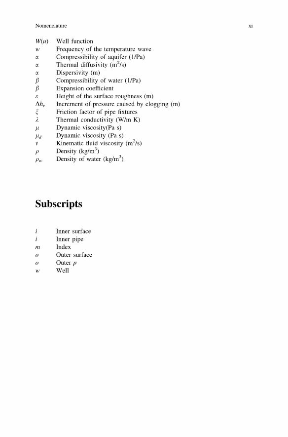
W(u) Well functionw Frequency of the temperature wavea Compressibility of aquifer (1/Pa)a Thermal diffusivity (m2/s)a Dispersivity (m)b Compressibility of water (1/Pa)b Expansion coefficiente Height of the surface roughness (m)Dhv Increment of pressure caused by clogging (m)n Friction factor of pipe fixturesk Thermal conductivity (W/m K)l Dynamic viscosity(Pa s)ld Dynamic viscosity (Pa s)m Kinematic fluid viscosity (m2/s)q Density (kg/m3)qw Density of water (kg/m3)

Subscripts

i Inner surfacei Inner pipem Indexo Outer surfaceo Outer pw Well

Nomenclature xi

Chapter 1Introduction

1.1 Energy Storage

1.1.1 Energy Demand

As fossil fuel resources such as oil, natural gas, and coal are increasingly lessavailable and more expensive, many energy conservation strategies become morefeasible. As global warming is also becoming one of the most urgent problems inthe world, people need to find a more efficient and economical way to utilizeenergy: not only in the field of energy production, transmission, distribution, andconsumption, but also in the area of energy storage (ES).

Today’s industrial civilizations are mainly based upon abundant and reliablesupplies of energy. In general, energy demands are not steady. Moreover, somethermal and electrical energy sources, such as solar energy, are not steady insupply. In cases where either supply or demand is highly variable, reliable energyavailability has in the past generally required energy production systems to belarge enough to supply the peak demand requirements. In all energy productionprocesses, it is economically inefficient to install production and distributionequipment with the capacity to accommodate for the maximum (short term)demand. Furthermore, productivity decreases when production equipment cannotoperate at full capacity in periods of reduced demand.

The basic idea behind thermal storage is to provide a buffer to balance fluc-tuations in supply and demand of energy (Nielsen 2003). Energy demand in thecommercial, industrial, and utility sectors fluctuates in cycles of 24 h periods (dayand night), intermediate periods (e.g. seven days) and according to seasons(spring, summer, autumn, winter). Therefore, the demand must be matched byvarious ES systems that operate synergistically.

Capital investments can sometimes be reduced if load management techniquesare employed to smooth power demands, or if ES systems are used to permit theuse of smaller power generating systems. The smaller systems operate at or nearpeak capacity, irrespective of the instantaneous demand for power, by storing the

K. S. Lee, Underground Thermal Energy Storage, Green Energy and Technology,DOI: 10.1007/978-1-4471-4273-7_1, � Springer-Verlag London 2013

1

excess converted energy during reduced demand periods for subsequent use inmeeting peak demand requirements. Although some energy is generally lost in thestorage process, ES often results in fuel conservation by utilizing more plentifulbut less flexible fuels such as coal and uranium in applications now requiringrelatively scarcer oil and natural gas.

Therefore, the applications of ES systems have an enormous potential for moreeffective use of energy equipment and for facilitating large-scale energy substi-tutions from the economic perspective. Systems for storing energy should there-fore reflect the cycles of energy demand, with either short-term, medium-term, orlong-term (seasonal) storage capacity.

ES has recently been developed to a point where it can have a significant impacton modern technology. In particular, it is important for the success of any irregularenergy source in meeting demand. For example, the need for storage for solarenergy applications is clear, especially when solar energy is least available,namely, at night and in winter. With the ES technology, it is possible to overcomethe mismatch between the energy production and consumption, lessen the stressedproduction load of the power plant at peak hours, and reduce consumers’ elec-tricity costs by avoiding higher peak hour tariffs.

Moreover, the ES is critically needed to reduce the various shortcomings ofrenewable energy technologies. Currently, most of the renewable energy sources,especially wind energy and solar energy, are time-based energy sources, whoseavailable energy densities are variable during different hours. ES systems can helpus avoid the irregular characteristics of renewable energy resources. The EStechnology can be used for storing the excess renewable energy in high productionhours, to make up for the possible shortage during low production hours, and tobetter integrate the energy generator into the local electricity grid.

For example, among the practical problems involved in solar energy systems isthe need for an effective means by which the excess heat collected during periods ofbright sunshine can be stored, preserved, and later released for utilization during thenight or other periods (Dincer 1999). Thermal energy storage (TES) can store solarheat in summer to be used in winter, or during sunny days to be used for cool nights.

TES can also help us in utilizing our natural energy resources such as summerheat or winter cold. These are essentially renewable resources, which have notbeen fully developed and utilized before. Heat in the summer results from solarradiation, heating the earth’s air, soil, and surface water. Storage in summer forwinter and/or in winter for summer is the seasonal storage system. These systemscontribute significantly to improve the efficiency of energy utilization. Thus theuse of fossil fuels and emissions of greenhouse gas or air pollutants such as CO2,SOx, and NOx can be reduced substantially. When natural cold from winter air canbe also stored and used for direct summer cooling, the need for electrical energyand expensive refrigerant with ozone depleting gases is reduced.

The main advantage of TES is that heat and cold may be moved in space andtime to utilize thermal energy that would otherwise be lost because it was availableat the wrong place at the wrong time. Although TES systems themselves do notsave energy, ES applications for energy conservation lead to the introduction of

2 1 Introduction

more efficient, integrated energy systems. TES therefore makes it possible to moreeffectively utilize renewable energy sources (solar, geothermal, or ambient) andwaste heat/cold recovery for space heating and cooling.

ES is considered an important energy conservation technology and, recently,increasing attention has been paid to its utilization, particularly for heating, ven-tilating, and air conditioning (HVAC) applications (Dincer 2002; Dincer and Rosen2007). Economic factors involved in the design and operation of energy conversionsystems have brought TES to the forefront. It is often useful to make provisions inan energy conversion system when the supply of and demand for thermal energy donot match. TES appears to be an advantageous option for adjusting the mismatchbetween the supply and demand of energy, and can contribute significantly tomeeting society’s needs for more efficient and environment friendly energy use.TES is a crucial component for successful thermal systems. An effective TES incursminimum thermal energy losses, leading to energy savings, while permitting thehighest possible recovery efficiency of the stored thermal energy.

Dincer and Rosen (2011) summarized the significant benefits from use of ESsystems as follows:

• reduced energy costs• reduced energy consumption• improved indoor air quality• increased flexibility of operation• reduced initial and maintenance costs• reduced equipment size• more efficient and effective utilization of equipment• conservation of fossil fuels (by facilitating more efficient energy use and/or fuel

substitution)• reduced pollutant emissions (e.g., CO2 and chlorofluorocarbons (CFCs))

1.1.2 Energy Storage Methods

Mechanical and hydraulic ES systems usually store energy by converting electricityinto energy of compression, elevation, or rotation. Pumped storage is proven, butquite limited in its applicability by site considerations. Compressed-air ES has beentried successfully in Europe, although limited applications appear in the UnitedStates. This concept can be applied on a large scale using depleted natural gas fieldsfor the storage reservoir. Alternatively, energy can be stored chemically ashydrogen in exhausted gas fields. Energy of rotation can be stored in flywheels, butadvanced designs with high-tensile materials appear to be needed to reduce theprice and volume of storage. A substantial energy loss of up to 50 % is generallyincurred by mechanical and hydraulic systems in a complete storage cycle becauseof inefficiencies.

1.1 Energy Storage 3

Reversible chemical reactions can also be used to store energy. There is agrowing interest in storing low-temperature heat in chemical form, but practicalsystems have not yet emerged. Another idea in the same category is the storage ofhydrogen in metal hydrides (lanthanum, for instance).

Electrochemical ES systems have better efficiencies but very high prices. Inten-sive research is now directed toward improving batteries, particularly by loweringtheir weight-to-storage capacity ratios, as needed in many vehicle applications.Following after lead-acid battery, sodium-sulfur, and lithium-sulfide alternatives,among others, are being extensively tested. A different type of electrochemicalsystem is the redox flow cell where charging and discharging is achieved throughreduction and oxidation reactions occurring in fluids stored in two separate tanks.

Thermal ES systems are varied, and include designed containers, undergroundaquifers and soils and lakes, bricks and ingots. Some systems using bricks areoperating in Europe. In these systems, energy is stored as sensible heat. Alternatively,thermal energy can be stored in the latent heat of melting in such materials as salts orparaffin. Latent storages can reduce the volume of the storage device by as much as100 times, but after several decades of research many of their practical problems havestill not been solved. Finally, electric energy can be stored in superconductingmagnetic systems, although the costs of such systems are high.

There are a number of areas in ES technology, as shown in Fig. 1.1 (Dincer andRosen 2011). Given the cost gap that needs to be spanned and the potentialbeneficial of ES applications, it is clear that a sustained ES development effort is inorder. For solar energy applications, advanced ES systems may not be needed foryears and decades. For the near term, many less expensive ES alternatives areavailable that should allow for the growth of solar energy use.

1.1.3 Energy Storage History

Man has used passively stored energy throughout history. Early examples arepeople who lived in natural or excavated caverns in rocks and soils. Suchdwellings were warm in the winter and cold in the summer because the seasonal

Fig. 1.1 A classification of energy storage methods (from Dincer and Rosen 2011)

4 1 Introduction

temperature variation does not penetrate deeply into the ground. It is also knownthat the buildings of the native people of Arizona and New Mexico in U.S.A.worked in the same way but on a diurnal basis. In this case the heat of the day didnot penetrate the wall until the coldest hour of the night while the cold of the nightwas cooling the inner wall surface during the warmest period of the day. There arealso many examples of ice cellars where ice was stored from the winter for coolingpurposes during the summer.

Small-scale short-term storage of hot water and ice was early made in warmwater bottles. Another example is electric water heaters in single family houses.Such heaters are motivated by power saving meaning that the heater takes manyhours to produce the necessary hot water, while the hot water is used duringshorter periods of the day.

One of the earliest types of technical energy stores were large water tanks toreduce the peak power demand. Such stores are now common in District Heatingsystems and also in solar applications. Storage systems are also needed in solarapplications because of the diurnal variation in solar intensity. In this way, thesolar energy is available after sunset. The variation in solar intensity also results inthe need for weekly and seasonal storage.

The interest in large-scale seasonal TES started with the oil crisis in the early1970s. At the beginning of seasonal storage research the long-term aim was tostore solar heat from the summer to the winter primarily for space heating.Industrial waste heat was another energy source of great potential. This is still truebut in recent years cooling has become an increasingly important issue and DistrictCooling systems are growing in Europe. So far, these systems have utilized pas-sively stored cold but now we see an increasing interest in large-scale seasonalcold storage systems.

1.1.4 Thermal Energy Storage

1.1.4.1 Introduction

Depending on the energy types, ES technology can be divided into two maincategories: TES and electrical ES (Cao 2010). Both are also the main energyconsumption types in our daily life. In theory, TES can be used to store electricalenergy, while the electrical storage can also be used to store thermal energy. Thereason that we seldom use the thermal storage technology to store electrical energyor use the electrical storage to store thermal energy is that the transformationbetween thermal and electrical energy will lead to the loss of a relatively largeamount of energy. In this book, we will focus on TES, especially on the under-ground thermal storage technology.

TES generally involves a temporary storage of high- or low-temperature thermalenergy for later use. Examples of TES are storage of solar energy for overnightheating, of summer heat for winter use, of winter ice for space cooling in summer,


and of heat or coolness generated electrically during off-peak hours for use duringsubsequent peak demand hours. Solar energy, unlike energy from fossil fuels, is notavailable all the time. Cooling loads, which nearly coincide with maximum levelsof solar radiation, are often present after sunset. This phenomenon is largely due tothe time lag between when objects are heated by solar energy and when they releasethe heat to the surrounding air. TES can help counterbalance this mismatch ofavailability and demand.

TES systems have been considered as one of the most crucial energy tech-nologies and recently, increasing attention has been paid to the utilization of thisessential technique. Energy may be stored in many ways, but since in much of theeconomy in many countries, energy is produced and transferred as heat, thepotential for TES warrants study in detail.

TES deals with the storage of energy by cooling, heating, melting, solidifying,or vaporizing a material. The thermal energy becomes available when the processis reversed. Storage by causing a material to rise or lower in temperature is calledsensible heat storage; its effectiveness depends on the specific heat of the storagematerial and, if volume is important, on its density. Sensible storage systemscommonly use rocks, ground, or water as the storage medium, and the thermalenergy is stored by increasing the storage-medium temperature.

Storage by phase change (the transition from solid to liquid or from liquid tovapor with no change in temperature) is a mode of TES known as latent heatstorage. Latent heat storage systems store energy in phase change materials(PCMs), with the thermal energy stored when the material changes phase, usuallyfrom a solid to a liquid. The specific heat of solidification/fusion or vaporizationand the temperature at which the phase change occurs are of design importance.Both sensible and latent TES also may occur in the same storage material. PCMsare either packaged in specialized containers such as tubes, shallow panels, plasticbags, and so on, or contained in conventional building elements (e.g., wall boardand ceiling) or encapsulated as self-contained elements.

The oldest form of TES probably involves harvesting ice from lakes and rivers andstoring it in well-insulated warehouses for use throughout the year for almost all tasksthat mechanical refrigeration satisfies today, including preserving food, coolingdrinks, and air-conditioning. The Hungarian parliament building in Budapest is stillair-conditioned, with ice harvested from Lake Balaton in the winter.

1.1.4.2 Thermal Energy

Thermal energy quantities differ in temperature. As the temperature of a substanceincreases, the energy content also increases. The energy required E to heat avolume V of a substance with density q from a temperature T1 to a temperature T2

is given by

E ¼ mC T2 � T1ð Þ ¼ qVC T2 � T1ð Þ ð1:1Þ

6 1 Introduction

where m is the material total mass and C is the specific heat of the substance.A given amount of energy may heat the same weight or volume of other substances,and increase the temperature. The specific heat is the amount of heat per unit massrequired to raise the temperature by one degree Kelvin. The value of C ranges fromabout 1 kcal/kg K or 4.186 kJ/kg K for water to 0.0001 kcal/kg K for somematerials at very low temperature. The specific heat of water is higher than anyother common substance. Water is both cheap and chemically stable. As a result,water plays a very important role in temperature regulation and has excellentproperties as a heat storage medium. Rock is another good sensible TES materialfrom the standpoint of cost, but its capacity is only half that of water (Dincer 2002).

The energy exchanged (released or absorbed) by a thermodynamic system thathas as its sole effect a change of temperature, is called the sensible heat. Latentheat, which is the amount of energy exchanged that is hidden, meaning it cannot beobserved as a change of temperature, is associated with the changes of state orphase change of a material. For example, during a phase change such as themelting of ice, the temperature of the system containing the ice and the liquid isconstant until all the ice has melted. The energy required for these changes toconvert ice into water, to change water into steam, and to melt paraffin wax iscalled the heat of fusion at the melting point and the heat of vaporization at theboiling point. The sensible heat for a given temperature change varies from onematerial to another. The latent heat also varies significantly between differentsubstances for a given type of phase change.

It is relatively straightforward to determine the value of the sensible heat forsolids and liquids, but the situation is more complicated for gases. If a gasrestricted to a certain volume is heated, both the temperature and the pressureincreases. The specific heat observed in this case is called the specific heat atconstant volume, Cv. If, instead the volume is allowed to vary and the pressure is

fixed, the specific heat at constant pressure, Cp, is obtained. The ratio Cp

Cvand the

fraction of the heat produced during compression can be saved, significantlyaffecting the storage efficiency.

1.1.4.3 Classification

Several TES technologies exist that can be used in combination with on-siteenergy sources to economically buffer the discrepancy between energy supply anddemand. TES is considered to be one of the most important technologies and,recently, increasing attention has been paid to utilizing TES in a variety of thermalengineering applications, ranging from heating to cooling and air conditioning.

Different criteria lead to various categories of TES technologies (Nordell 2000).Based on the temperature level of stored thermal energy, the TES can be dividedinto ‘‘heat storage’’ and ‘‘cool storage’’ (Hasnain 1998a, b). Based on the timelength of stored thermal heat, it can be classified as ‘‘short term’’ and ‘‘long term’’.


There are basically three types of thermal storage devices being investigated atpresent by the international research society and some industrial players: that is,‘‘sensible (specific) heat storage’’, ‘‘latent heat storage (PCMs)’’, and ‘‘thermo-chemical heat storage’’ (Sharma et al. 2009). Sensible heat storage, in which thetemperature of the storage material varies with the amount of energy stored, andlatent heat storage, which makes use of the energy stored when a substance changesfrom one phase to another by melting (as from ice to water) (Hasnain 1998a).

Sensible heat storage is affected by raising the temperature of the storagemedium. Thus, it is desirable for the storage medium to have high specific heatcapacity, long-term stability under thermal cycling, compatibility with its con-tainment and, most importantly, low cost. The high specific heat capacity C canhave direct impact on the amount of stored thermal energy based on Eq. 1.1. Thelong-term stability assures the low degradation of the heat storage material afterhundreds or thousands of thermal cycling. Good compatibility with its containmentis the requirement for both the heat storage material and the containment, and isone of the main factors of the total cost of the storage system. The cost of thesensible heat storage solution mainly depends on the characteristics of the storagematerial. It is very common to utilize very cheap materials such as water, rocks,pebbles, sands, etc., as the storage medium (Cao 2010).

Sensible heat storage may be classified on the basis of the heat storage media asliquid media storage (like water, oil-based fluids, molten salts, etc.) and solidmedia storage (like rocks, metals, and others) (Hasnain 1998a). Sensible heat EShas the advantage of being relatively cheap but the energy density is low and thereis a gliding discharging temperature. Latent heat storage is a particularly attractivetechnique, since it provides a high ES density. It has the capacity to store heat aslatent heat of fusion at a constant temperature corresponding to the phase transitiontemperature of the PCMs.

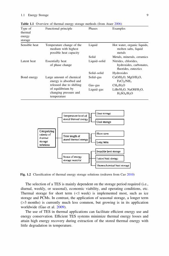
The sorption or thermochemical reactions provide thermal storage capacity.The basic principle is: AB ? heat$ A ? B; using heat a compound AB is brokeninto components A and B which can be stored separately; bringing A and Btogether AB is formed and heat is released. The storage capacity is the heat ofreaction or free energy of the reaction. Ataer (2006) gives an overview of TESmethods as shown in Table 1.1.

As shown in Fig. 1.2, TES technologies can be classified with different criteria,leading to various categories. If the criterion is based on the temperature level ofstored thermal energy, the thermal storage solutions can be divided into ‘‘heatstorage’’ and ‘‘cool storage’’. If based on the time length of stored thermal heat, itcan be divided into ‘‘short term’’ and ‘‘long term’’. If based on the state of ESmaterial, it can be divided into ‘‘sensible heat storage’’, ‘‘latent heat storage’’ and‘‘thermochemical heat storage’’.

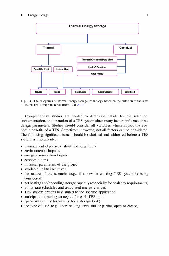
In Zalba et al. (2003)’s paper, a useful classification was given on the sub-stances used for TES, shown in Fig. 1.3. Cao (2010) also provided a similarschematic (Fig. 1.4) of the categories based on the criterion of state of the ESmaterial.

8 1 Introduction

The selection of a TES is mainly dependent on the storage period required (i.e.,diurnal, weekly, or seasonal), economic viability, and operating conditions, etc.Thermal storage for short term (\1 week) is implemented most, such as icestorage and PCMs. In contrast, the application of seasonal storage, a longer term([3 months) is currently much less common, but growing is in its applicationworldwide (Gao et al. 2009).

The use of TES in thermal applications can facilitate efficient energy use andenergy conservation. Efficient TES systems minimize thermal energy losses andattain high energy recovery during extraction of the stored thermal energy withlittle degradation in temperature.

Table 1.1 Overview of thermal energy storage methods (from Ataer 2006)

Type ofthermalenergystorage

Functional principle Phases Examples

Sensible heat Temperature change of themedium with highestpossible heat capacity

Liquid Hot water, organic liquids,molten salts, liquidmetals

Solid Metals, minerals, ceramicsLatent heat Essentially heat

of phase changeLiquid–solid Nitrides, chlorides,

hydroxides, carbonates,fluorides, eutectics

Solid–solid HydroxidesBond energy Large amount of chemical

energy is absorbed andreleased due to shiftingof equilibrium bychanging pressure andtemperature

Solid–gas CaO/H2O, MgO/H2O,FeCl2/NH3

Gas–gas CH4/H2OLiquid–gas LiBr/H2O, NaOH/H2O,

H2SO4/H2O

Fig. 1.2 Classification of thermal energy storage solutions (redrawn from Cao 2010)


1.1.5 Various Aspects of TES

This section is mainly based on Dincer and Rosen (2001)’s discussion on the varioustechnical, economical, energetic, exergetic, and environmental aspects of TES.

1.1.5.1 Economic Aspects

ES technology is benign to the environment. This is, however, not a good enoughreason, as long as the environmental advantages have not been given an eco-nomical value. The only valid reason for ES in a market economy (like it or not) isthat it is more cost effective to store energy from one time to another, than toproduce it later when needed. This implies that the storage energy must be cheaperwhen injected than the value of energy when it is recovered. This price differencemust be big enough to cover the cost of investment, maintenance, operation, andenergy losses. Today, there are many economically feasible storage applications.

TES-based systems are usually economically justifiable when the annualizedcapital and operating costs are less than those for primary generating equipmentsupplying the same service loads and periods. TES is often installed to reduce initialcosts of other plant components and operating costs. Lower initial equipment costsare usually obtained when large durations occur between periods of energy demand.Secondary capital costs may also be lower for TES-based systems. For example, theelectrical service equipment size can sometimes be reduced when energy demand islowered. In comprehensive economic analyses of systems including and notincluding TES, initial equipment and installation costs must be determined, usuallyusing manufacturer data, or estimated. Operating cost savings and net overall costsshould be assessed using life cycle costing or other suitable methods for deter-mining the most beneficial among multiple systems. TES use can enhance theeconomic competitiveness of both energy suppliers and building owners.

Fig. 1.3 Classification of energy storage materials (from Zalba et al. 2003)

10 1 Introduction

Comprehensive studies are needed to determine details for the selection,implementation, and operation of a TES system since many factors influence thesedesign parameters. Studies should consider all variables which impact the eco-nomic benefits of a TES. Sometimes, however, not all factors can be considered.The following significant issues should be clarified and addressed before a TESsystem is implemented:

• management objectives (short and long term)• environmental impacts• energy conservation targets• economic aims• financial parameters of the project• available utility incentives• the nature of the scenario (e.g., if a new or existing TES system is being

considered)• net heating and/or cooling storage capacity (especially for peak day requirements)• utility rate schedules and associated energy charges• TES system options best suited to the specific application• anticipated operating strategies for each TES option• space availability (especially for a storage tank)• the type of TES (e.g., short or long term, full or partial, open or closed)

Fig. 1.4 The categories of thermal energy storage technology based on the criterion of the stateof the energy storage material (from Cao 2010)


1.1.5.2 Environmental Aspects

TES systems can contribute significantly to meet society’s desires for more envi-ronment friendly energy use and reduce environmental impacts, especially in buildingheating and cooling, space power, and utility applications. By reducing energy use,TES systems provide significant environmental benefits by conserving fossil fuelsthrough increased efficiency and/or fuel substitution, and by reducing emissions ofsuch pollutants as CO2, SO2, NOx and CFCs.

TES can impact air emissions in buildings by reducing quantities of ozonedepleting CFC and HCFC refrigerants in chillers and emissions from fuel-firedheating and cooling equipment. TES helps reduce CFC use in two main ways.First, since cooling systems with TES require less chiller capacity than conven-tional systems; they use fewer or smaller chillers and correspondingly lessrefrigerant. Second, using TES can offset the reduced cooling capacity thatsometimes occurs when existing chillers are converted into more benign refrig-erants, making building operators more willing to switch refrigerants.

1.1.5.3 Sustainability Aspects

A reliable supply of energy is generally agreed to be a necessary but not sufficientrequirement for development within a civilized society. Furthermore, sustainabledevelopment demands a sustainable supply of energy resources. Sustainabledevelopment within a society requires a supply of energy resources that, in the longterm, is readily and sustainably available at reasonable cost and can be utilized forall required tasks without causing negative societal impacts.

Supplies of such energy resources as fossil fuels and uranium are generallyacknowledged to be limited. Other energy sources such as sunlight, wind, andfalling water are generally considered renewable and therefore sustainable over therelatively long term. Wastes convertible to useful energy forms and biomass fuelsare also usually viewed as sustainable energy sources. Another implication of thesustainability is that sustainable development requires that energy resources beused as efficiently as possible. In this way, society maximizes the benefits itderives from utilizing its energy resources, while minimizing the correspondingnegative impacts such as environmental damage. This implication acknowledgesthat all energy resources are to some degree finite, so that greater efficiency inutilization allows such resources to contribute to make development moresustainable. Even for energy sources that may eventually become inexpensive andwidely available, increases in energy efficiency will likely remain sought to reducethe resource requirements for energy and material to create and maintain systemsand devices to harvest the energy, and to reduce the associated environmentalimpacts. TES systems can contribute to increased sustainability as they can helpextend supplies of energy resources, improve costs, and reduce environmental andother negative societal impacts.

12 1 Introduction

Sustainability objectives often lead local and national governments to incor-porate environmental considerations into energy planning. The need to satisfybasic human needs and aspirations, combined with increasing world population,make successful implementation of sustainable development increasingly needed.Requirements for achieving sustainable development in a society include:

• provision of information about and public awareness of the benefits ofsustainability

• investments• environmental education and training• appropriate energy and ES strategies• availability of renewable energy sources and clear technologies• a reasonable supply of financing• monitoring and evaluation tools.

References

Ataer ÖE (2006) Storage of thermal energy. In: Gogus YA (ed) Encyclopedia of life supportsystems. Eolss Publishers, Oxford

Cao S (2010) State of the art thermal energy storage solutions for high performance buildings,Master’s thesis, University of Jyväskylä, Finland

Dincer I (1999) Evaluation and selection of energy storage systems for solar thermal applications.Int J Energy Res 23(7):1017–1028

Dincer I (2002) Thermal energy storage as a key technology in energy conservation. Int J EnergyRes 26(7):567–588

Dincer I, Rosen MA (2001) Energetic, exergetic, environmental and sustainability aspects ofthermal energy storage systems for cooling capacity. Appl Therm Eng 21(11):1105–1117

Dincer I, Rosen MA (2007) Energetic, exergetic, environmental and sustainability aspects ofthermal energy storage systems. In: Paksoy HÖ (ed) Thermal energy storage for sustainableenergy consumption, fundamentals, case studies, and design. Springer, Dordrecht

Dincer I, Rosen MA (2011) Thermal energy storage: systems and applications, 2nd edn. Wiley,New York

Gao Q, Li M, Yu M, Spitler JD, Yan YY (2009) Review of development from GSHP to UTES inChina and other countries. Renew Sustain Energy Rev 13(6–7):1383–1394

Hasnain SM (1998a) Review on sustainable thermal energy storage technologies, part I: heatstorage materials and techniques. Energy Convers Manag 39(11):1127–1138

Hasnain SM (1998b) Review on sustainable thermal energy storage technologies, part II: coolthermal storage. Energy Convers Manag 39(11):1139–1153

Nielsen K (2003) Thermal energy storage, a state-of-the-art. NTNU, TrondheimNordell B (2000) Large-scale thermal energy storage. WinterCities’2000, Energy and Environment,

Luleå, Sweden, 14 Feb 2000Sharma A, Tyagi VV, Chen CR, Buddhi D (2009) Review on thermal energy storage with phase

change materials and applications. Renew Sustain Energy Rev 13(2):318–345Zalba B, Marin JM, Cabeza LF, Mehling H (2003) Review on thermal energy storage with phase

change: materials, heat transfer analysis and applications. Appl Therm Eng 23(3):251–283


Chapter 2Underground Thermal Energy Storage

2.1 Introduction

Nature provides storage systems between the seasons because thermal energy ispassively stored into the ground and groundwater by the seasonal climate changes.Below a depth of 10–15 m, the ground temperature is not influenced and equalsthe annual mean air temperature. Therefore, average temperature of the ground ishigher than the surface air temperature during the winter and lower during thesummer. Consequently, the ground and groundwater are suitable media for heatextraction during the winter and cold extraction during the summer (Nordell et al.2007). Such extraction systems are often used both for heating during the winterand for cooling during the summer. This means that the extracted heat is rechargedduring the summer and it becomes a storage system. If the heat demand is less orgreater than the cooling demand additional storage might be needed. Systemsusing natural underground sites for storing thermal energy are called undergroundthermal energy storage (UTES) systems.

Because large volume is necessary for seasonal purposes, heat storage systemsare in most cases in the ground or placed close to the surface. The application ofseasonal storage, a longer term ([3 months), is currently much less common, butits application is growing worldwide. UTES is one form of TES and it can keep alonger term and even seasonal thermal energy storage. When large volumes areneeded for thermal storage, underground thermal energy storage systems are mostcommonly used. It has become one of the most frequently used storage technol-ogies in North America and Europe.

UTES systems started to be developed in the 1970s for the purpose of energyconservation by increasing energy efficiency. These systems store thermal energyfrom natural heat and/or cold in air, soil and water, solar energy, and waste heatfrom any mechanical process for seasonal purposes. It is possible to use thesummer heat for heating in winter and winter cold for cooling in summer withUTES systems. With the use of UTES systems, the consumption of conventionalfossil fuels was reduced by enabling the usage of alternative energy sources.


15

Replacement of conventional heating systems also resulted in decreasing emis-sions of CO2, SO2, and NOx emitted from the combustion of fossil fuel.Mechanical cooling devices using ozone-depleting substances such as CFCs can bealso reduced. If fully exploited and utilized, UTES systems can play an importantrole in reducing emissions that lead to global warming and ozone depletion.

2.1.1 Ground Temperature

Measurements have shown that the ground temperature below a certain depthremains relatively constant throughout the year. Temperature fluctuations at theearth’s surface influence shallow groundwater temperatures to depths of approx-imately 10 m. Between depths of 10 and 20 m, that is, maximum depth of annualcyclic variation, groundwater temperatures remain relatively stable at temperaturestypically 1–2 �C higher than local mean annual temperatures. Below these depths,groundwater temperatures gradually increase at a rate of roughly 1 �C per 35 mdepth toward the earth’s interior which is termed the geothermal gradient.

Measurements of ground temperature have a long history. Lavoisier, Frenchphysicist and chemist, installed a thermometer in the deep vaults beneath the ParisObservatory in the seventeenth century and proved the constant temperatures atapproximately 20 m below street level. Many years later, in 1778, Buffon pub-lished observations with that thermometer, and Humboldt noted in 1799 a meantemperature of 12 �C with annual variation of not more than 0.024 �C in the Parisunderground. In the nineteenth century, more measurements followed, the mostnotable are those at the Royal Observatory in Edinburgh, UK. The decrease ofseasonal temperature variations with depth and the constant temperatures in thesubsurface had been demonstrated (Sanner and Nordell 1998).

The temperature fluctuations at the surface of the ground are moderated as thedepth of the ground increases because of the high thermal inertia of the soil. Also,there is a time gap between the temperature fluctuations at the ground surface andin the ground. The observation of relatively constant ground temperature can beexplained by these two facts. Therefore, at a sufficient depth, the ground tem-perature is always higher than that of the outside air in winter and is lower insummer. The temperature variation of the ground at various depths in summer(August) and winter (January) is shown in Fig. 2.1 (Florides and Kalogirou 2007).The graph shows actual ground temperatures as measured in a borehole drilled forthis purpose in Nicosia, Cyprus. As can be expected, the temperature is shown tobe nearly constant below a depth of 5 m for the year round.

The difference in temperature between the outside air and the ground can beutilized as a preheating in winter and precooling in summer by operating a groundheat exchanger. Also, because of the higher efficiency of a heat pump than con-ventional natural gas or oil heating systems, a heat pump may be used in winter toextract heat from the relatively warm ground and pump it into the conditioned space.

16 2 Underground Thermal Energy Storage

In summer, the process may be reversed and the heat pump may extract heat fromthe conditioned space and send it out to a ground heat exchanger that warms therelatively cool ground.

2.1.2 Historical Development

Technology of underground thermal energy storage has a 40-year history, whichbegan with cold storage in aquifers in China. Outside China, the idea of UTESstarted with more theoretical work in the early 1970s.

Interest in UTES systems increased rapidly in the 1980s and several pilot anddemonstration plants were built, in combination with solar thermal energy, withwaste heat or heat pumps. Some of the plants listed were purely experimental,others operated successfully for some years and a few are still in use today. Thetemperature level ranged from around 0 �C to more than 150 �C in someexperiments.

2.1.3 Advantages

The advantages of UTES systems compared to the conventional ones are significantand summarized by Saljnikov et al. (2006) as follows:

• enormous reserves of energy in the nature that could be stored in this mannerand later used for various purposes (heating or cooling)

• low operation costs and high long-term profitability (Reduction of electricitycosts for operation of cooling machines and plants is nearly 75 %. The period oftime during which the additional investment costs become paid off is shorterthan five years.)

• protection of the environment (There is no pollution of the environment and thesources are recoverable.)

• possible utilization of the abandoned boreholes that were drilled for differentpurposes

Fig. 2.1 Temperature variations with depth (from Florides and Kalogirou 2007)

2.1 Introduction 17

2.2 Classification

There are several concepts as to how the underground can be used for thermalenergy storage depending on geological, hydrogeological, and other site conditions.UTES systems can be classified according to:

• storage temperature (low or high)• storage purpose (heating, cooling, or combined heating and cooling)• storage technology (open/aquifer, closed/boreholes, or other techniques such as

caverns)• application (residential, commercial, or industrial)

2.2.1 Storage Temperature

In the low-temperature UTES, storage temperatures range from around 0 �C to amaximum of 40–50 �C. The technology includes thermal energy storage forcooling, combined heating and cooling, and low-temperature heating such as heatsource for heat pumps. The boundary between this type of storage and mereground source heat pumps (GSHP) is vague. Large GSHP installations with acentral borehole- or well-field are in fact special types of UTES plants. To beconsidered a UTES system in this overview, a GSHP system should have a heatdissipation to (or extraction from) the surrounding ground of no more than 25 % ofthe annual thermal energy turnover. UTES exhibits substantial environmentaladvantages in reducing emissions of greenhouse and ozone-depleting gases.

Cold storage systems with heat pumps were already described in the IEA HeatPump Centre Newsletter in 1992. Sanner and Nordell (1998) show the variousalternatives of underground cold storage as presented in Fig. 2.2. These systemsalways substitute chillers which, compared to thermal storage, have a relativelyhigh energy demand to drive compressors or absorption cycles.

When using heat pumps in combination with underground cold storage, threeoperation modes are possible as seen in Fig. 2.3 (Sanner and Nordell 1998). Theyuse either modes one and two (direct cooling only), mode one and three (coolingwith heat pump only), or all three modes (direct cooling in spring and during lowdemand, cooling by heat pump in summer or during peak demand).

Underground heat storage in the temperature range below 40 �C is usually doneto increase the heat-source temperature of heat pumps. Charging sources for thestorage include surface water, solar collectors, pipes below paved surfaces, hot airin glassed spaces, low-temperature waste heat, or by other sources.

High-temperature UTES systems have storage temperatures above 40–50 �C.Typical heat sources for these systems are solar collectors or waste heat. Varioussystem layouts are possible. Heat pumps are either used at the end of the storageunloading period, when temperatures drop, or for achieving higher supply


temperatures. Hydrochemical, biological, and geotechnical problems increase withincreasing temperatures. Experiments showed that UTES with supply temperaturesabove 100 �C were not successful. Methods for water treatment have beendeveloped for high temperature ATES, but further work is required. The newAnnex 12 of the IEA program on Energy Conservation through Energy Storage(IEA ECES) addresses the specific problems of high temperature UTES.

Fig. 2.2 Classification of underground cold storage alternatives (from Sanner and Nordell 1998)

Fig. 2.3 Operational modes of cold storage UTES with heat pumps (from Sanner and Nordell1998)

2.2 Classification 19

2.2.2 Storage Technology

The basic types of underground thermal energy storage systems under the defi-nition of this book can be divided into two groups (Sanner 2001; Novo et al. 2010):

• Systems where a technical fluid (water in most cases) is pumped through heatexchangers in the ground, also called ‘‘closed’’ systems (BTES).

• Systems where groundwater is pumped out of the ground and injected into theground by the use of wells, or in underground caverns, also known as ‘‘open’’systems (ATES, CTES).

Among the UTES systems developed since the 1970s, there are:

• aquifer thermal energy storage (ATES)• borehole thermal energy storage (BTES)• cavern thermal energy storage (CTES)• pit storage• water tank

Aquifer thermal energy storage uses natural water in a saturated and permeableunderground layer called an aquifer as the storage medium. Thermal energy istransferred by extracting groundwater from the aquifer and by reinjecting it at achanged temperature at a separate well nearby. Aquifer thermal energy storage isthe least expensive of all natural UTES options.

Borehole thermal energy storage consists of vertical heat exchangers deeplyinserted below the soil from 20 to 300 m deep, which ensures the transfer ofthermal energy toward and from the ground (clay, sand, rock, etc.). Many projectsare about the storage of solar heat in summer for space heating of houses or offices.Ground heat exchangers are also frequently used in combination with heat pumps(geothermal heat pump), where the ground heat exchanger extracts/transfers lowtemperature heat from/to the soil. The flexibility of this technology at almost anyground conditions has made BTES systems one of the most popular forms of UTES.

Cavern thermal energy storage uses water in large, open, underground cavernsin the subsoil to serve as thermal energy storage systems. Caverns used can benatural or man made, including depleted oil or natural gas fields, or abandonedmine tunnels and shafts. These storage technologies are technically feasible, butthe actual application is still limited, because extremely specific site conditions arerequired, which are often not available (Zizzo 2009).

Water tank and pit storage, also called man-made aquifers, are artificial struc-tures built below ground, like buried tanks, or close to the surface to circumventhigh excavation cost. They will, then, need to be insulated both on the top and alongthe walls, at least down to some depth. Hydrogeological conditions at the specificsite are not as relevant as in the other concepts. Table 2.1 summarizes some of thecharacteristics of the main seasonal storage concepts (Schmidt et al. 2003).

Figure 2.4 shows the most common thermal storage systems, namely, ATES,BTES, and CTES (Nordell et al. 2007). The two most promising technologies are


storage in aquifers (ATES) and through borehole heat exchangers (BTES). Theseconcepts have already been introduced as commercial systems on the energymarket in several countries. Other options are rarely applied commercially.

Advantages of closed systems are the separation from aquifers and fewerproblems related to water chemistry. An advantage of open systems is higher heattransfer capacity of a well compared to a borehole. This makes ATES usually thecheapest option if the subsurface is hydrogeologically and hydrochemically suited.

2.3 Characteristics of Underground Storage Systems

This section is based on the works of EU Commission SAVE Program and NordicEnergy Research (2004) which summarized the characteristics of UTES forground source cooling in terms of efficiency, availability, applications, tempera-ture, humidity, and load. The concept can be also applied to heating with thermalenergy storage.

Table 2.1 Comparison of storage concepts (from Schmidt et al. 2003)

Storageconcept

Hot water Gravel water Duct Aquifer

Storagemedium

Water Gravel water Ground material(soil/rock)

Ground material (sand/water or gravel)

Heatcapacity

(kWh/m3)

60–80 30–50 15–30 30–40

Storagevolumefor 1 m3

water

equivalent 1 m3 1.3–2 m3 3–5 m3

2–3 m3

Geologicalrequirements

Stable groundconditions

Preferably nogroundwater

5–15 m deep

Stable groundconditions

Preferably nogroundwater

5–15 m deep

Drillable groundGroundwater

favorableHigh heat capacityHigh thermal

conductivityLow hydraulic

conductivity(K \ 1 9 10-10

m/s)Natural groundwater

flow \1 m/y30–100 m deep

Natural aquifer layerwith high hydraulicconductivity(K [ 1 9 10-5 m/s)

Confining layers on topand below

No or low naturalgroundwater flow

Suitable waterchemistry at hightemperatures

Aquifer thickness20–50 m deep

2.2 Classification 21

2.3.1 Efficiency Benefits

Convention cooling machines, which provide comfort and process cooling, arenormally driven by electricity with an average seasonal performance factor (SPF),in the range of 2–4. This means that an input of 1 kWh of electricity is needed forevery 2–4 kWh of cold.

By storing natural sources of cold seasonally or from night till day, the usage ofelectricity for production of cold can be markedly reduced. To store, recover, anduse these sources for free cooling will drastically increase the performance factorcompared to conventional systems. ATES systems will normally work with a SPFof 30–50 when it comes to the cooling part of the system, while BTES has aslightly lower SPF of 20–30. This means that for 1 kWh of electricity, 20–50 kWhof cold is produced.

To have a proper thermal performance, any UTES system has to be of a certainminimum size. If not, the stored cold will be lost in temperature quality due tothermal losses. This may not be a critical factor in the cases when the coolingtemperature is at a rather high level and close to the initial ground temperature.Still, any losses will reduce the performance factor. In certain applications, i.e.,district cooling, the production temperature is essential and can have a significantimpact on the efficiency.

Fig. 2.4 Schematic representation of the most common UTES systems, ATES, BTES, and CTES(redrawn from Nordell et al. 2007)


2.3.2 Availability

UTES systems can replace almost any type of conventional cooling and heating inalmost any application sector. It is possible to find a system that suits to thegeological and hydrogeological conditions at a given site. If one cannot find asuitable aquifer for ATES, it is practically always possible to use boreholes tocreate a BTES system. Also, pits in the soil or caverns (CTES) may sometimes beconsidered as an alternative option.

The underground conditions will always be the most important factor in anUTES project. However, there may be other types of conditions that affect thechoice of system. For example in the case of ATES, the relevant aquifer mayhave a priority for drinking water supply and hence will not be approved as storagefacility. In some cases, aquifers are too small compared to the expected need forstorage, or there are legal or environmental difficulties that limit the availability.

Wells and boreholes used for UTES do not take much space once they havebeen constructed. In many cases, they may even be hidden under the surface andplaced below parking lots, gardens, or buildings. However, during construction,the required space for drilling rigs and side equipment has to be considered.

2.3.3 Potential Applications Sectors

From a global perspective and considering all different types of climate, there areseveral potential applications for UTES. These applications include

• air conditioning in residential, commercial, and institutional buildings andoccasionally industrial buildings

• process cooling in manufacturing industries, food processing, telecom applica-tions, IT facilities, and electric generation with combustion technologies

• cooling for food preservation and quality maintenance• cooling and heating for growing some agricultural products in greenhouses• cooling for fish farming in dams

2.3.4 Temperature Levels

The different applications all have different requirements when it comes to thesupply temperatures, which vary from +6 up to +15 �C for air conditioningsystems. For the other application sectors, the temperature will in most cases be atequal or at a higher level. The temperature difference between flow and return istypically 6 �C.

2.3 Characteristics of Underground Storage Systems 23

ATES systems can easily meet any temperature requirement down to 4–5 �C,but operates better at higher temperatures, whereas BTES systems in theory can beused also for temperatures below the freezing point. However, in practice BTESsystems are more cost-effective for a supply temperature above 8–10 �C.

2.3.5 Humidity Aspects

Normal requirement for ventilation air is in the range of 40–60 % relativehumidity (RH). This means that the air sometime has to be dehumidified inclimates with high humidity.

In Scandinavian and North European countries, the humidity is seldom aproblem. Hence, air conditioning can take place also with a relatively high coolingsupply temperature. That speaks in favor of UTES systems, which normallyproduce a higher supply temperature at the later stage of the cooling season.

The relative humidity for food preservation of vegetables and fruit should ingeneral be kept above 70 % to prevent drying. In such applications, the UTESconcepts have proven to be very useful as they can provide a high supply temperature.

2.3.6 Load Coverage

For comfort air conditioning, the load will mainly be dependent on the buildingstructure, the envelope, and the function of the building. Normally, it is not aproblem to meet any load with ATES systems. However, for BTES systems it isoften too expensive to design the system to cover cooling peaks. Therefore, it isrecommended that systems are designed for the base load and then cut the peakswith a heat pump.

2.4 Advantages and Limitations of UndergroundStorage Systems

Requirements for energy efficiency of buildings are growing constantly, as theawareness of the environmental effects of energy use is increasing. Heating, cooling,and lighting of buildings cause more than one-third of the world’s primary energyuse. Thus, the building stock contributes significantly to the energy-related envi-ronmental problems. Space heating is by far the largest energy end use of householdsand offices, but energy use for cooling in households and the tertiary sector is nowincreasing rapidly and is for this sector alone expected to amount to more than70,000 GWh in 2020. The technical saving potential of UTES technologies is esti-mated to be as high as 85 % of the cooling energy, meaning a saving potential of


59,500 GWh per year in whole EU if all cooling systems would be changed intoUTES systems. Use of the UTES technologies offers main advantages compared toconventional systems. Naturally, there are also some limitations that should be takeninto account, when designing the thermal system. Common advantages and limita-tions of all UTES technologies for seasonal storage are summarized (EU CommissionSAVE Program and Nordic Energy Research 2004).

2.4.1 Advantages

• Energy savingsExperiences have shown that up to 100 % of the cooling demand can be coveredby natural sources combined with use of UTES systems. It corresponds toaround 70–85 % saving on electricity used for cooling systems (compared toconventional chillers). Heat pumps (electric or heat driven) can be used togetherwith UTES systems to cover both cooling and heating needs. Then total energysavings would be even higher.

• Environmental impactsThe saving of electricity will be also beneficial to the environment with feweremissions of harmful gases to the atmosphere, especially the ones causing globalwarming, depletion of the ozone layer, and acid rain (preferably CO2, SOx, and NOx).

• ProfitabiltyThe economic potential in terms of straight payback time is usually veryfavorable. The payback period for UTES systems is often less than five years.However, even with a payback period of more than 10 years, life cycle costassessments show that investments on the UTES are very profitable. Because thesystems, especially BTES based, are long lasting, UTES delivers savings formany years. By careful analysis of actual demands, the investment cost may beless than for a traditional (often oversized) cooling plant.

• Esthetics and noiseThe noiseless operation and esthetical superiority of the invisible UTES systemsare usually highly appreciated.

• Health aspectsThe risk of Legionella bacteria problems is eliminated as the systems are closedand separated from the distribution system. Thus, they will produce no wateraerosols in air, which might appear in traditional systems with cooling towers.

2.4.2 Limitations

There are also a number of limitations and different condition to consider beforethe decision to construct a UTES system is taken. ATES systems are not as easy toconstruct as BTES systems, and need more maintenance and preinvestigations.

2.4 Advantages and Limitations of Underground Storage Systems 25

If the conditions are favorable, payback times are typically short, ranging normally2–5 years. ATES systems cannot be constructed in all geological conditions, andhence they sometimes require extensive preinvestigations, which have to be takeninto account and budgeted from the early design phase. The process of obtaining apermit can be complex and time consuming for the first plant in the region, andmany restrictions in relation to protection of groundwater resources and envi-ronmental impact assessment may diminish possibilities. Some ATES plants haveshown different kinds of operational problems, although most of them can behandled with simple measures. One major identified problem is clogging of wells.In most cases, the clogging processes can be avoided by a proper well and systemdesign and operation.

BTES systems are generally easier to construct and operate, need limitedmaintenance, and have extraordinary durability. Moreover, BTES systems usuallyrequire only simple procedures for authority approvals. Yet, their payback timesare relatively long compared to ATES systems, normally 6–10 years. This is dueto expensive borehole investments and the fact that BTES systems normally needsome other sources to cover the peak load situations.

References

EU Commission SAVE Programme and Nordic Energy Research (2004) Pre-design guide forground source cooling systems with thermal energy storage. COWI A/S, Denmark

Florides G, Kalogirou S (2007) Ground heat exchangers-a review of systems, models andapplications. Renew Energy 32(15):2461–2478

Nordell B, Grein M, Kharseh M (2007) Large-scale utilisation of renewable energy requiresenergy storage. In: International conference for renewable energies and sustainableDevelopment (ICRESD_07), Algeria, 21–24 May 2007

Novo AV, Bayon JR, Castro-Fresno D, Rodriguez-Hernandez J (2010) Review of seasonal heatstorage in large basins: water tanks and gravel-water pits. Appl Energy 87(2):390–397

Saljnikov A, Goricanec D, Kozic Ð, Krope J, Stipic R (2006) Borehole and aquifer thermalenergy storage and choice of thermal response test method. In: Proceedings of the 4thWSEAS international conference on heat transfer, thermal engineering and environment,Elounda, Greece, 21–23 Aug 2006

Sanner B (2001) A different approach to shallow geothermal energy–underground thermal energystorage (UTES). International Summer School on Direct Application of Geothermal Energy

Sanner B, Nordell B (1998) Underground thermal energy storage with heat pumps, IEA HeatPump Cent. Newsl 16(2):10–14

Schmidt T, Mangold D, Muller-Steinhagen H (2003) Seasonal thermal energy storage inGermany. ISES Solar World Congress, Göteborg, Sweden, 14–19 June 2003

Zizzo R (2009) Designing an optimal urban community mix for an aquifer thermal energy storagesystem. M.S. Thesis, University of Toronto, Toronto, Canada


Chapter 3Basic Theory and Ground Properties

Deng (2004) introduced a theoretical background on underground thermal energysystems in his dissertation on standing column wells. The contents in this chapterare mainly based on Deng’s (2004) dissertation.

3.1 Basic Physical Mechanism

Above the water table lies the unsaturated zone, where voids or pores betweenrocks are usually only partially filled with water, the remainder being occupiedwith air. Water is held in the unsaturated zone by molecular attraction, and it willnot flow toward or enter a well. In the saturated zone, which lies below the watertable, all the openings in the rocks are full of water that may move through theaquifer to streams, springs, or wells from which water is being withdrawn (seeFig. 3.1).

The energy transport in the ground outside of the well is through a porousmedia called an aquifer. An ‘‘aquifer’’ is defined as a geologic formation, group offormations, or part of a formation that contains sufficient saturated permeablematerial to yield economical quantities of water to wells and springs. The aquifercan be considered as a porous medium that consists of a solid phase and aninterconnected void space totally filled with groundwater.

Transport of groundwater occurs only through the interconnected voids. Heat istransported both in the solid matrix and in the void system, forming a coupled heattransfer process with conduction and advection by moving groundwater. Thegoverning steady-state, one-dimensional equations for heat and fluid flow aregiven by Fourier’s law and Darcy’s law, which are identical in the form:

Fourier’s law:

q ¼ �kdT

dxð3:1Þ


27

where q is heat flux (W/m2); k is the thermal conductivity of the ground (W/m K).Darcy’s law:

u ¼ �Kdh

dxð3:2Þ

where u is the specific discharge or Darcy flux (volume flow rate per unit of cross-sectional area) (m/s); K is the hydraulic conductivity of ground (m/s); h is thehydraulic head (m).

The specific discharge u is related to average linear groundwater velocity v by:

v ¼ u

nð3:3Þ

where n is the porosity, which, for a given cross-section of a porous medium, is theratio of the pore area to the cross-sectional area.

3.1.1 Hydrological Flow in the Aquifer

The first fundamental law governing groundwater flow is the continuity equation,which expresses the principle of mass conservation (De Smedt 1999). Consider theflow of groundwater through an elementary control volume of porous mediumaround a point with Cartesian coordinates (x, y, z) as shown in Fig. 3.2.

The principle of mass conservation on the control volume implies that the netresult of inflow minus outflow is balanced by the change in storage versus time.

Fig. 3.1 Occurrence of groundwater in rocks (http://capp.water.usgs.gov/GIP/gw_gip/how_occurs.html)

28 3 Basic Theory and Ground Properties

http://capp.water.usgs.gov/GIP/gw_gip/how_occurs.html


� o qvxð Þox

þo qvy

� �

oyþ o qvzð Þ

oz

� �¼ o qnð Þ

otð3:4Þ

The time rate of change of mass stored in the control volume is defined as thetime rate of change of fluid mass in storage, expressed as after some manipulation.

o qnð Þot¼ qSs

oh

otð3:5Þ

By applying Darcy’s law to the law of mass conservation in a control volume,the governing equation defining the hydraulic head distribution in the porousmedium can be derived as:

Ssoh

ot¼ o

oxiKij

oh

oxi

� �þ R ð3:6Þ

where Ss is the specific storage (m-1 [ft-1]). Specific storage is the amount ofwater per unit volume of a saturated formation that is stored or expelled fromstorage owing to compressibility of the mineral skeleton and the pore water perunit change in head (Fetter 2001). It is also called the elastic storage coefficientand expressed as:

Ss ¼ qg aþ nbð Þ ð3:7Þ

q is the density of water (kg/m3); g is the acceleration of gravity (m/s2); a is thecompressibility of aquifer (1/(N/m2)); b is the compressibility of water (1/(N/m2));Kij is the hydraulic conductivity tensor (m/s); R is the source/sink ([s-1]).

Fig. 3.2 Mass conservationin a reference elementaryvolume

3.1 Basic Physical Mechanism 29

3.1.2 Hydrological Flow in Borehole

The flow in the borehole of UTES systems is often non-Darcy flow where therelationship between the flux and gradient is nonlinear. By introducing theeffective hydraulic conductivity (EHC) Keff , we are still able to use Eq. 3.2 todescribe the water flow in the borehole just replacing Kij with Keff . It is recom-mended to use the following formulas:

Keff ¼K Darcy flow in the aquiferd2qwg

32l laminar pipe flow in the borehole2gduf transitional and turbulent flow in the borehole

8><

>:ð3:8Þ

where d is the diameter (m); l is the dynamic viscosity (Pa s); u is the averagewater velocity in the borehole (m/s); f is the friction factor.

3.1.3 Heat Transfer Mechanism

Different mechanisms are used to describe heat transfer in the aquifer (porousmedium) and heat transfer in the borehole of UTES systems. Figure 3.3 shows allthe heat transfer mechanisms in the standing column well (SCW) system which isthe most complicated system.

3.1.3.1 Heat Transfer in the Aquifer

There are several heat transfer processes affecting the heat transferred through anaquifer:

• heat conduction through the fluid phase• heat conduction through the solid phase• particle to particle radiation• heat convection from the fluid phase to the solid phase• convection through the fluid phase (advection).

Figure 3.4 shows the relationship between the actual thermal conductivity andthe four mechanisms that contribute to it. None of the first three processes isaffected by fluid flow, and the last two processes are dependent on fluid velocity.At large velocities, the last two processes are dominant.

It is generally assumed that the solid and fluid phases in the aquifer are at thesame temperature by thermal equilibrium. Therefore, one can consider the tem-perature as an average temperature of both phases. An effective thermal conduc-tivity keff of porous medium is expressed with classical mixing rule (Lee and Yang1998):


keff ¼ nkl þ 1� nð Þks ð3:9Þ

where kl is the thermal conductivity of the fluid (W/m K); ks is the thermalconductivity of the solid (W/m K). In general, the more porous the medium, thelower the effective thermal conductivity, because water has a lower thermalconductivity than most solids.

The advection–diffusion equation can be used where enthalpy is thermal energycontent only. Heat is transported by advection in the liquid phase and by bothadvection and diffusion in both phases. Dividing by the volume the energy balanceequation of the control volume, taking constants out of the derivative and sim-plifying gives

qCp

� �cv

oT

otþ qlCplVi

oT

oxi¼ keff

o2T

ox2i

þ Q ð3:10Þ

Fig. 3.3 Heat transfer mechanisms in SCW systems (redrawn from Deng 2004)


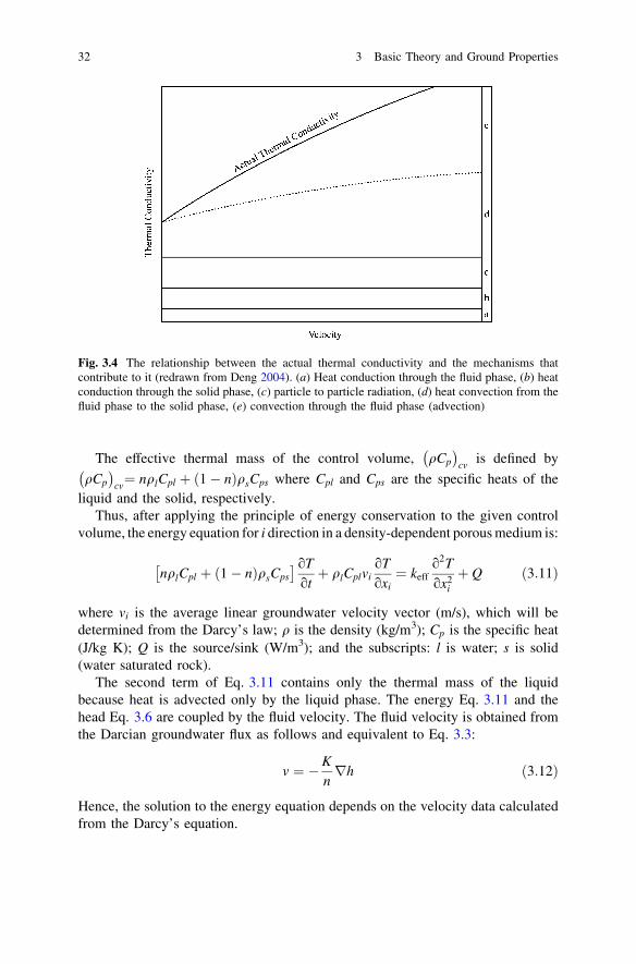
The effective thermal mass of the control volume, qCp

� �cv

is defined by

qCp

� �cv¼ nqlCpl þ 1� nð ÞqsCps where Cpl and Cps are the specific heats of the

liquid and the solid, respectively.Thus, after applying the principle of energy conservation to the given control

volume, the energy equation for i direction in a density-dependent porous medium is:

nqlCpl þ 1� nð ÞqsCps

� oT

otþ qlCplvi

oT

oxi¼ keff

o2T

ox2i

þ Q ð3:11Þ

where vi is the average linear groundwater velocity vector (m/s), which will bedetermined from the Darcy’s law; q is the density (kg/m3); Cp is the specific heat(J/kg K); Q is the source/sink (W/m3); and the subscripts: l is water; s is solid(water saturated rock).

The second term of Eq. 3.11 contains only the thermal mass of the liquidbecause heat is advected only by the liquid phase. The energy Eq. 3.11 and thehead Eq. 3.6 are coupled by the fluid velocity. The fluid velocity is obtained fromthe Darcian groundwater flux as follows and equivalent to Eq. 3.3:

v ¼ �K

nrh ð3:12Þ

Hence, the solution to the energy equation depends on the velocity data calculatedfrom the Darcy’s equation.

Fig. 3.4 The relationship between the actual thermal conductivity and the mechanisms thatcontribute to it (redrawn from Deng 2004). (a) Heat conduction through the fluid phase, (b) heatconduction through the solid phase, (c) particle to particle radiation, (d) heat convection from thefluid phase to the solid phase, (e) convection through the fluid phase (advection)


3.1.3.2 Heat Transfer in the Borehole

Heat transfer in the borehole of SCW systems is characterized in the r direction byconvection from the pipe walls and borehole wall, plus advection at the boreholesurface, and in the z direction by advection only. The thermal model for theborehole can be described by a series of resistance networks as shown in Fig. 3.5.

An energy balance on the water in the annular region can be formulated in eachz plane. The energy balance equation can be written as:

Fig. 3.5 The borehole thermal model (redrawn from Deng 2004)


d mCpTa;z

� �

dt¼qconvection; suction tube þ qconvection; discharge tube þ qconvection; rock

þ qadvection; rock þ qadvection; annulus

ð3:13Þ

Through mathematical manipulations, the left-hand side of Eq. 3.13 can bereduced to:

d mCpTa;z

� �

dt¼ dmCpTa;z

dtþ mCpdTa;z

dt¼ _mdtCpTa;z

dtþ mCpdTa;z

dt

¼ _mCpTa;z þ mCpdTa;z

dt¼ _mgwCpTa;z þ _mannulusCpTa;z þ VqCp

dTa;z

dtð3:14Þ

The right-hand side of Eq. 3.13 can be modified to:

RHS ¼qconvection; suction tube þ qconvection; discharge tube þ qconvection; rock

þ _mgwCpTrock þ _mannulusCpTannulus

ð3:15Þ

Thus, the energy balance Eq. 3.13 can be rewritten as:

VqCpdTa;z


þ _mgwCp Trock � Ta;z

� �þ _mannulusCp Tannulus � Ta;z

� � ð3:16Þ

After the new definitions, Eq. 3.16 can be written as:

VqCpdTa;z


þ qadvection; rock þ qadvection; annulus

ð3:17Þ

where

qadvection; rock ¼ _mgwCp Trock � Ta;z

� �

qadvection; annulus ¼ _mannulusCp Tannulus � Ta;z

� �

and Ta;z is the water temperature in the annular region at node z (�C); V is thevolume of water in the annular region (m3); q is the density of water in the annularregion (kg/m3); Cp is the specific heat of water (J/kg K); _mgw is the mass flow rateof groundwater in/out of the borehole (kg/s); _mannulus is the mass flow rate of waterin the annulus of the borehole (kg/s).

Similarly, for the water in each of the tubes the energy balance is given by:

VqCpdTtube;z

dt¼ qconvection; annular region þ qadvection; tube ð3:18Þ

where Ttube;z is the water temperature in the tube (discharge tube or suction tube) atnode z (�C).


The advection heat transfer rates in Eqs. 3.15 and 3.18 can be given by:

qadvection;n ¼ _mCp Tn � Ta;z

� �ð3:19Þ

where _m is the mass flow rate of the water (kg/s); n refers to each of the rock andannular fluid at nodes z� 1 and zþ 1.

The convection heat transfer rates in Eqs. 3.15 and 3.18 are given by:

qconvection;n ¼1

RmTm � Ta;z

� �ð3:20Þ

where R is the thermal resistance (�C/W); m is an index referring to the dischargetube, the suction tube, or the rock.

The thermal resistance in Eq. 3.20 is defined as the following:

Rm ¼1

Ai;m

1hi;mþ ri

kpipe

lnri

ro

� �þ ri

ro

1ho

� �� ð3:21Þ

where A is the area (m2); r is the radius (m); h is the heat transfer coefficient (W/m2

K); and subscript: i is the inner surface, o is the outer surface.The heat transfer coefficient, h, is defined as:

h ¼ Nukwater

Dhð3:22Þ

where Dh is the hydraulic diameter (m).

3.1.3.3 Convective Heat Transfer in the Borehole

The literature review regarding convective heat transfer correlations in annularspaces suggests that the difference between concentric pipe configurations andeccentric pipe configurations may not be significant. Also, the correlationsapplicable to eccentric configurations are limited, and most of them are in tabularforms, not explicit correlations. Hence, the correlations will be based on concentricconfigurations. In the standing column well, to obtain good heat transfer, theannular area in the well is usually smaller than the area inside the dip tube, so thevelocity near the wall is high enough to produce turbulent flow. Here, the attentionis put on the turbulent flow.

The circular duct correlations for friction factors will be used. For smoothsurfaces, the Techo’s correlation has least relative error compared to the Prandtl,

Kármán, Nikuradse (PKN) empirical formula 1 ffiffifp ¼ 1:7372 ln

�Re

ffiffiffifp� 0:3946ð ÞÞ.

1ffiffiffifp ¼ 1:7372 ln

Re1:964 ln Re� 3:8215

for 104\Re\107 ð3:23Þ


For rough surface, the explicit equation with least relative error compared to the

Colebrook-White empirical formula 1 ffiffifp ¼ 3:48� 1:7372 ln e

aþ 9:35Re

ffiffifp

� �� is given:

1ffiffiffifp ¼ 3:48� 1:7372 ln

eaþ 16:2426

Reln A2

� �for all values of Re and

ea

ð3:24Þ

where f is the Fanning friction factor; Re is the Reynolds number, Re ¼ DhVm ; V is

the fluid velocity (m/s); m is the kinematic fluid viscosity (m2/s); e is the height of

the surface roughness (m); A2 ¼eað Þ

1:1098

6:0983 þ 7:149Re

� �0:8981, a is the radius of duct (m).

In the above formula, the laminar equivalent diameter, Dl, can be substituted forthe hydraulic diameter, Dh for more accuracy.

Dl

Dh¼

1þ r �2 þ 1�r�2

ln r�1� r�ð Þ2

ð3:25Þ

where r� ¼ riro

; ro and ri are the radius of outer and inner pipes, respectively (m);

Dh is the hydraulic diameter which is defined as 4 9 area/wet perimeter (here,Dh ¼ 2ðro � riÞ) (m).

The circular duct correlations for Nusselt number could be used for both theinner and outer walls of the pipes in standing column well systems. But thehydraulic diameter (Do � Di) should be used in those correlations. The correlationby Gnielinski is used for smooth surfaces such as the discharge and suction tube:

Nu ¼f2 Re� 1000ð Þ Pr

1þ 12:7 f2

� �12 Pr

23�1

� � ð3:26Þ

For rough surfaces such as the borehole wall, the following correlation may beused because the range of Reynolds number, Re, in this correlation is very wide(i.e., Re [ 2,300):

Nu ¼f2 Re� 1000ð Þ Pr

1þ f2

� �12 17:42� 13:77 Pr0:8

t

� �Re0:2

e Pr0:5�8:48� ð3:27Þ

where Pr is the Prandtl number:

Prt¼

1:01� 0:09 Pr0:36 for 1� Pr� 1451:01� 0:11 ln Pr for 145\Pr� 1; 8000:99� 0:29 ln Prð Þ

12 for 1,800\Pr� 12; 500

8<

:;

Ree is the roughness Reynolds number, Ree ¼Re

ffiffif2

p

De

.


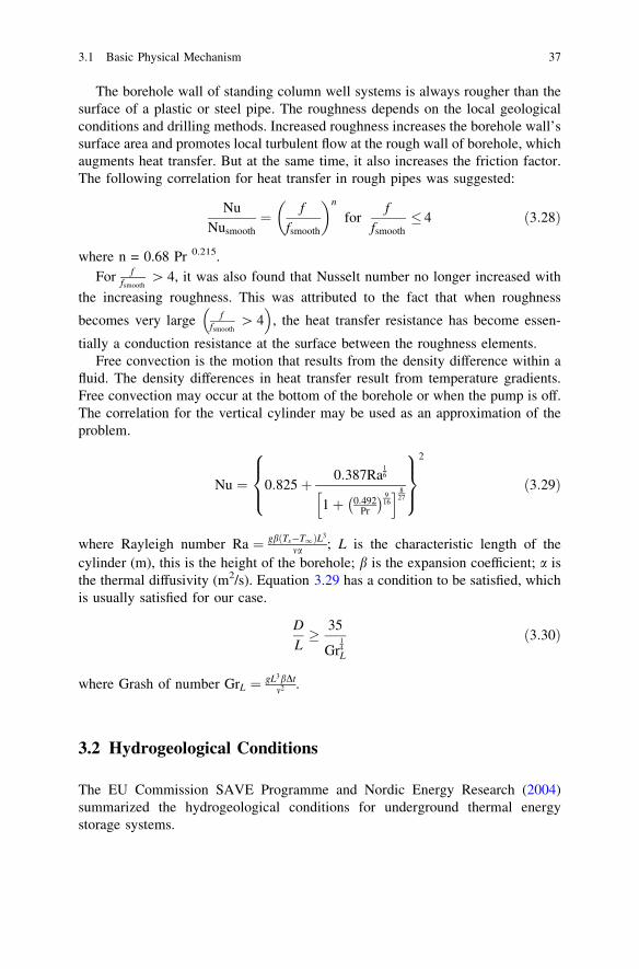
The borehole wall of standing column well systems is always rougher than thesurface of a plastic or steel pipe. The roughness depends on the local geologicalconditions and drilling methods. Increased roughness increases the borehole wall’ssurface area and promotes local turbulent flow at the rough wall of borehole, whichaugments heat transfer. But at the same time, it also increases the friction factor.The following correlation for heat transfer in rough pipes was suggested:

NuNusmooth

¼ f

fsmooth

� �n

forf

fsmooth

� 4 ð3:28Þ

where n = 0.68 Pr 0.215.For f

fsmooth[ 4, it was also found that Nusselt number no longer increased with

the increasing roughness. This was attributed to the fact that when roughness

becomes very large ffsmooth

[ 4� �

, the heat transfer resistance has become essen-

tially a conduction resistance at the surface between the roughness elements.Free convection is the motion that results from the density difference within a

fluid. The density differences in heat transfer result from temperature gradients.Free convection may occur at the bottom of the borehole or when the pump is off.The correlation for the vertical cylinder may be used as an approximation of theproblem.

Nu ¼ 0:825þ 0:387Ra16

1þ 0:492Pr

� � 916

h i 827

8><

>:

9>=

>;

2

ð3:29Þ

where Rayleigh number Ra ¼ gb Ts�T1ð ÞL3

ma ; L is the characteristic length of thecylinder (m), this is the height of the borehole; b is the expansion coefficient; a isthe thermal diffusivity (m2/s). Equation 3.29 has a condition to be satisfied, whichis usually satisfied for our case.

D

L� 35

Gr14L

ð3:30Þ

where Grash of number GrL ¼ gL3bDtm2 .

3.2 Hydrogeological Conditions

The EU Commission SAVE Programme and Nordic Energy Research (2004)summarized the hydrogeological conditions for underground thermal energystorage systems.


3.2.1 Aquifer Systems

The aquifer’s hydraulic conductivity (K) is a measure of the ability of the porousgeologic media to transmit water. It is of first-order significance in design andevaluation of aquifer thermal energy storage systems, and is dependent on the sizeand shape of the pores. Hydraulic conductivity varies over a wide range of over 13orders of magnitude. Hydraulic conductivity multiplied by aquifer thickness(b) equals aquifer transmissivity (T), which is a measure of the rate at which watermoves through a unit width of the aquifer under a unit hydraulic gradient. A highhydraulic conductivity (and transmissivity) is desired to produce the largest vol-ume of water from a well with the least drawdown of groundwater level. However,low hydraulic conductivity is desirable for decreased regional groundwatervelocity and prevention of excessive tilting of the thermocline from viscosity/buoyancy effects in high-temperature ATES systems. Isotropic aquifer mediahaving the same hydraulic conductivity in all directions are desirable to obtainmaximum water supply from a well with minimum drawdown. But, conversely,anisotropic conditions with vertical hydraulic conductivity being much less thanhorizontal hydraulic conductivity are desirable for high-temperature ATES sys-tems to resist tilting of the thermocline.

If total volume (VT ) of the rock is divided into the volumes of solid and voids(Vv), porosity (n) of geologic media is defined as n ¼ Vv

VT. With regard to the storage

and movement of water in a porous medium, effective porosity considering onlythe system of interconnected interstices is important. The porosity of the aquifermatrix is an important consideration in ATES systems because it determines theamount of heated or chilled water that can be stored per unit volume of the aquifer.Porosity also is important because it is one factor that controls the average linearvelocity of groundwater flow. Average linear velocity of groundwater in a porousmedium is proportional to the hydraulic conductivity and gradient by Darcy’s lawand inversely proportional to the porosity as indicated in Eq. 3.12.

Areal aquifer boundaries and thickness determine the volume available forstorage of heat or chill. Aquifer volume generally is much greater than the requiredstorage volume, but boundary location may be of interest if the proposed ATESstorage site is near zones of recharge or discharge, or on the periphery of agroundwater system.

Thermal characteristics of the aquifer are important in determining the heatcapacity of the system and heat transfer out of the storage volume. Thermalconductivity is the quantity of heat conducted in unit time across an element ofsurface under a given thermal gradient. Porous geologic materials, saturated withwater, do not vary widely in thermal conductivity values. Basically, earth materialsare good insulators under ATES conditions, and differences in their thermalconductivities are relatively small. Thus, thermal conductivity is of second-orderimportance in hydrogeologic characterization. Thermal capacity (specific heat) ofa material is the quantity of heat required to produce a unit change of temperature


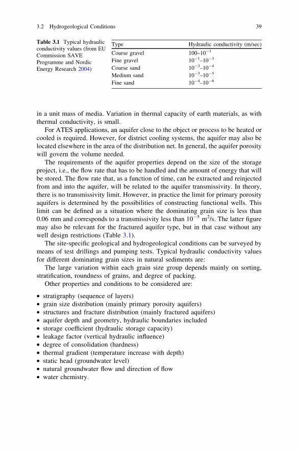
in a unit mass of media. Variation in thermal capacity of earth materials, as withthermal conductivity, is small.

For ATES applications, an aquifer close to the object or process to be heated orcooled is required. However, for district cooling systems, the aquifer may also belocated elsewhere in the area of the distribution net. In general, the aquifer porositywill govern the volume needed.

The requirements of the aquifer properties depend on the size of the storageproject, i.e., the flow rate that has to be handled and the amount of energy that willbe stored. The flow rate that, as a function of time, can be extracted and reinjectedfrom and into the aquifer, will be related to the aquifer transmissivity. In theory,there is no transmissivity limit. However, in practice the limit for primary porosityaquifers is determined by the possibilities of constructing functional wells. Thislimit can be defined as a situation where the dominating grain size is less than0.06 mm and corresponds to a transmissivity less than 10-5 m2/s. The latter figuremay also be relevant for the fractured aquifer type, but in that case without anywell design restrictions (Table 3.1).

The site-specific geological and hydrogeological conditions can be surveyed bymeans of test drillings and pumping tests. Typical hydraulic conductivity valuesfor different dominating grain sizes in natural sediments are:

The large variation within each grain size group depends mainly on sorting,stratification, roundness of grains, and degree of packing.

Other properties and conditions to be considered are:

• stratigraphy (sequence of layers)• grain size distribution (mainly primary porosity aquifers)• structures and fracture distribution (mainly fractured aquifers)• aquifer depth and geometry, hydraulic boundaries included• storage coefficient (hydraulic storage capacity)• leakage factor (vertical hydraulic influence)• degree of consolidation (hardness)• thermal gradient (temperature increase with depth)• static head (groundwater level)• natural groundwater flow and direction of flow• water chemistry.

Table 3.1 Typical hydraulicconductivity values (from EUCommission SAVEProgramme and NordicEnergy Research 2004)

Type Hydraulic conductivity (m/sec)

Course gravel 100–10-1

Fine gravel 10-1–10-3

Course sand 10-3–10-4

Medium sand 10-3–10-5

Fine sand 10-4–10-6

3.2 Hydrogeological Conditions 39

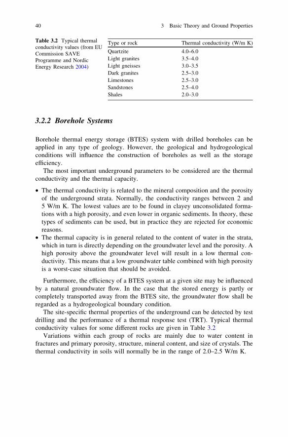
3.2.2 Borehole Systems

Borehole thermal energy storage (BTES) system with drilled boreholes can beapplied in any type of geology. However, the geological and hydrogeologicalconditions will influence the construction of boreholes as well as the storageefficiency.

The most important underground parameters to be considered are the thermalconductivity and the thermal capacity.

• The thermal conductivity is related to the mineral composition and the porosityof the underground strata. Normally, the conductivity ranges between 2 and5 W/m K. The lowest values are to be found in clayey unconsolidated forma-tions with a high porosity, and even lower in organic sediments. In theory, thesetypes of sediments can be used, but in practice they are rejected for economicreasons.

• The thermal capacity is in general related to the content of water in the strata,which in turn is directly depending on the groundwater level and the porosity. Ahigh porosity above the groundwater level will result in a low thermal con-ductivity. This means that a low groundwater table combined with high porosityis a worst-case situation that should be avoided.

Furthermore, the efficiency of a BTES system at a given site may be influencedby a natural groundwater flow. In the case that the stored energy is partly orcompletely transported away from the BTES site, the groundwater flow shall beregarded as a hydrogeological boundary condition.

The site-specific thermal properties of the underground can be detected by testdrilling and the performance of a thermal response test (TRT). Typical thermalconductivity values for some different rocks are given in Table 3.2

Variations within each group of rocks are mainly due to water content infractures and primary porosity, structure, mineral content, and size of crystals. Thethermal conductivity in soils will normally be in the range of 2.0–2.5 W/m K.

Table 3.2 Typical thermalconductivity values (from EUCommission SAVEProgramme and NordicEnergy Research 2004)

Type or rock Thermal conductivity (W/m K)

Quartzite 4.0–6.0Light granites 3.5–4.0Light gneisses 3.0–3.5Dark granites 2.5–3.0Limestones 2.5–3.0Sandstones 2.5–4.0Shales 2.0–3.0


3.3 Determination of Hydrogeological Properties

Successful design and operation of a UTES system depend on three elements: (1)the presence of a suitable aquifer for ground-water supply and energy storage; (2)the availability of a source of free or low-cost thermal energy; and (3) a temporalmismatch between thermal energy availability and thermal energy use.

Element 1 is usually the most difficult component of an ATES system to assessquantitatively. In their paper, Hall and Raymond (1992) presented a practical andeconomic method for characterizing hydrogeologic systems for ATES applica-tions. The method combines conventional hydrologic testing with single-wellgeochemical tracer tests.

Aquifer characterization is important to the engineering design of an ATESinstallation; that is, the aquifer must be considered as one important component ofthe ATES heating or cooling plant. However, unlike the pumps, heat exchangers,and other mechanical components of the system, the aquifer cannot be changed tomeet design specifications. Thus, to some degree, the ATES plant must bedesigned to accommodate the aquifer.

For example, the capacity of the aquifer to accept or yield water limits the flowrate that can be used in an ATES plant. Also, the effective porosity of the aquiferaffects the volume of aquifer required to store a given volume of heated or chilledwater. These affect the size of an ATES well field. The direction and rate ofgroundwater flow similarly affects the size, shape, and operation of the well field.

3.3.1 Step-Drawdown Tests

Boonstra (1999a) and American Society for Testing and Materials (1999) provideda summary on the drawdown in a pumped well and drawdown test. The drawdownin a pumped well consists of two components: the aquifer losses and the welllosses. Aquifer losses are the head losses that occur in the aquifer where the flow islaminar. They are time dependent and vary linearly with the well discharge. Thedrawdown s1 corresponding to this linear aquifer loss can be expressed as

s1 ¼ B1 rw;tð ÞQ ð3:31Þ

where B1 is the linear aquifer loss coefficient in day/m2. This coefficient can becalculated from the well flow equations. For confined aquifers for example, it canbe expressed as

B1 rw;tð Þ ¼W uð Þ4pT

ð3:32Þ

where u ¼ r2wS

4Tt. From the results of aquifer-test analyses, the values for transmis-sivity T and storativity S can be used to calculate B1 values as function of rw and t.

3.3 Determination of Hydrogeological Properties 41

Well losses are divided into linear and nonlinear head losses. Linear well lossesare caused by damaging the aquifer during drilling and completion of the well.They comprise head losses due to the compaction of the aquifer material duringdrilling; head losses due to plugging of the aquifer with drilling mud, whichreduces the permeability near the bore hole; head losses in the gravel pack; andhead losses in the screen. The drawdown corresponding to this linear well loss canbe expressed as

s2 ¼ B2Q ð3:33Þ

where B2 is the linear well loss coefficient in day/m2.Among the nonlinear well losses are the friction losses that occur inside the

well screen and in the suction pipe where the flow is turbulent, and head losses thatoccur in the zone adjacent to the well where the flow is usually also turbulent. Allthese losses responsible for the drawdown inside the well are much greater thanone would expect on theoretical grounds. The drawdown s3 corresponding to thisnonlinear well loss can be expressed as

s3 ¼ CQP ð3:34Þ

where C is the nonlinear well loss coefficient in dayP/m3P-1, and P is an exponent.The general equation describing the drawdown in a pumped well as function ofaquifer/well losses and discharge rate thus reads as

sw ¼ B1 þ B2ð ÞQþ CQP ¼ BQþ CQP ð3:35Þ

where sw ¼ s1 þ s2 þ s3. The value of P can vary between 1.5 and 3.5 and may beeven higher in fractured rock aquifers. The value of P ¼ 2 is, however, widelyaccepted. Values of the three parameters B, C, and P in Eq. 3.35 can be found fromthe analysis of so-called step-drawdown tests.

A step-drawdown test is a single-well test in which the well is pumped at a lowconstant-discharge rate until the drawdown within the well stabilizes. Thepumping rate is then increased to a higher constant discharge rate and the well ispumped until the drawdown stabilizes once more. This process is repeated throughat least three steps, which should all be of equal duration, say, a few hours each(Fig. 3.6).

In step-drawdown analyses, use is made of so-called diagnostic plots. Values ofswQ versus Q are therefore plotted on arithmetic paper, where sw represents the

drawdown at the end of each step. Various configurations of diagnostic plots arethen possible:

• The points fall on a horizontal line. This implies that swQ ¼ B. Equation 3.35

reduces to

sw ¼ BQ ð3:36Þ


Hence, there are no nonlinear well losses. This situation is only encountered withvery low pumping rates. The well will act differently if the pumping rates areincreased.• The points fall on a straight line under a slope. This means that sw

Q ¼ Bþ CQ.

Equation 3.35 then reduces to

sw ¼ BQþ CQ2 ð3:37Þ

Equation 3.37 is known as the Jacob’s equation. Based on this equation, Jacob(1947) developed an analysis method to calculate the values of B and C.• The points fall on a curved line, i.e., P 6¼ 2 in Eq. 3.35. When a concave curve

can be drawn through the points, it implies that P [ 2 and for a convex curve thatP\2. For these cases, an analysis method was developed to calculate the valuesof B, C, and P. Both analysis methods may be applied to confined, unconfined,and leaky aquifers.

Fig. 3.6 Principles of a step-drawdown test (from Boonstra 1999a)


3.3.2 Well Flow Equations

As summarized by Boonstra (1999b), the well flow equations presented weredeveloped under the following common assumptions and conditions: (1) theaquifer has a seemingly infinite areal extent; (2) the aquifer is homogeneous,isotropic, and of uniform thickness over the area influenced by the test; (3) prior topumping, the hydraulic head is horizontal (or nearly so) over the area that will beinfluenced by the test; (4) the pumped well penetrates the entire thickness of theaquifer and thus receives water by horizontal flow; (5) the aquifer is pumped at aconstant-discharge rate; (6) the water removed from storage is dischargedinstantaneously with decline of head; and (7) the diameter of the pumped well issmall, i.e., the storage inside the well can be neglected.

Theis was the first to develop an equation for unsteady-state flow whichintroduced the time factor and the storativity. He noted that when a fully pene-trating well pumps an extensive confined aquifer at a constant rate, the influence ofthe discharge extends outward with time. The rate of decline of head, multiplied bythe storativity and summed over the area of influence, equals the discharge. TheTheis equation, which was derived from the analogy between the flow ofgroundwater and the conduction of heat, is written as

s r; tð Þ ¼ Q

4pT

Z 1

u

e�y

ydy ¼ Q

4pTW uð Þ ð3:38Þ

with

u ¼ r2S

4Tt

where s r; tð Þ is the drawdown in m measured in a well, Q is the constant welldischarge in m3/day, T is the transmissivity of the aquifer in m2/day, W uð Þ is thedimensionless Theis well function, r is the distance in m from the pumped well,S is the dimensionless storativity of the aquifer, and t is the time in days sincepumping started. In Fig. 3.7, the Theis well function W uð Þ is plotted versus 1

u onsemi-log paper. This figure shows that, for large values of 1

u, the Theis wellfunction exhibits a straight-line segment. The Jacob method is based on thisphenomenon. For the straight-line segment, Eq. 3.39 can be approximated by

s r; tð Þ ¼ 2:3Q

4pTlog

2:25Tt

r2Sð3:39Þ

In most handbooks on this subject, the condition to use Eq. 3.39 is taken as1u [ 100. This limiting condition can often be relaxed to 1

u [ 10.When a confined aquifer is pumped, the cone of depression will continuously

deepen and expand. Even at late pumping times, the water levels in the piezometerswill never stabilize to a real steady state. Although the water levels continue todrop, the cone of depression will eventually deepen uniformly over the area


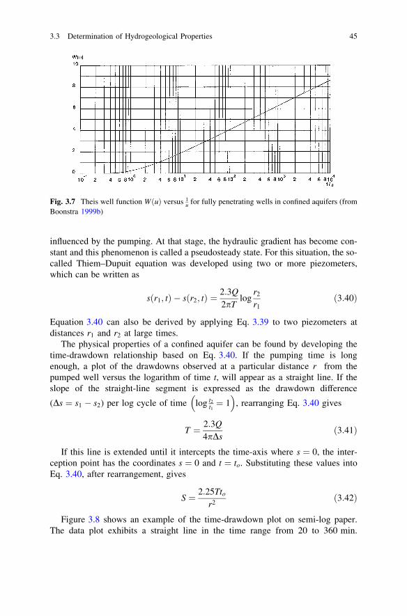
influenced by the pumping. At that stage, the hydraulic gradient has become con-stant and this phenomenon is called a pseudosteady state. For this situation, the so-called Thiem–Dupuit equation was developed using two or more piezometers,which can be written as

s r1; tð Þ � s r2; tð Þ ¼ 2:3Q

2pTlog

r2

r1ð3:40Þ

Equation 3.40 can also be derived by applying Eq. 3.39 to two piezometers atdistances r1 and r2 at large times.

The physical properties of a confined aquifer can be found by developing thetime-drawdown relationship based on Eq. 3.40. If the pumping time is longenough, a plot of the drawdowns observed at a particular distance r from thepumped well versus the logarithm of time t, will appear as a straight line. If theslope of the straight-line segment is expressed as the drawdown difference

(Ds ¼ s1 � s2) per log cycle of time log t2t1¼ 1

� �, rearranging Eq. 3.40 gives

T ¼ 2:3Q

4pDsð3:41Þ

If this line is extended until it intercepts the time-axis where s ¼ 0, the inter-ception point has the coordinates s ¼ 0 and t ¼ to. Substituting these values intoEq. 3.40, after rearrangement, gives

S ¼ 2:25Tto

r2ð3:42Þ

Figure 3.8 shows an example of the time-drawdown plot on semi-log paper.The data plot exhibits a straight line in the time range from 20 to 360 min.

Fig. 3.7 Theis well function W uð Þ versus 1u for fully penetrating wells in confined aquifers (from

Boonstra 1999b)


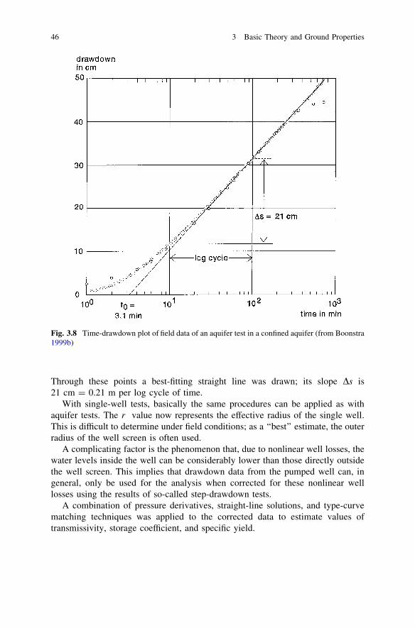
Through these points a best-fitting straight line was drawn; its slope Ds is21 cm = 0.21 m per log cycle of time.

With single-well tests, basically the same procedures can be applied as withaquifer tests. The r value now represents the effective radius of the single well.This is difficult to determine under field conditions; as a ‘‘best’’ estimate, the outerradius of the well screen is often used.

A complicating factor is the phenomenon that, due to nonlinear well losses, thewater levels inside the well can be considerably lower than those directly outsidethe well screen. This implies that drawdown data from the pumped well can, ingeneral, only be used for the analysis when corrected for these nonlinear welllosses using the results of so-called step-drawdown tests.

A combination of pressure derivatives, straight-line solutions, and type-curvematching techniques was applied to the corrected data to estimate values oftransmissivity, storage coefficient, and specific yield.

Fig. 3.8 Time-drawdown plot of field data of an aquifer test in a confined aquifer (from Boonstra1999b)


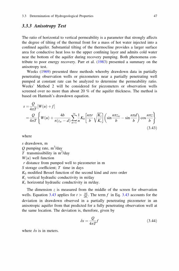
3.3.3 Anisotropy Test

The ratio of horizontal to vertical permeability is a parameter that strongly affectsthe degree of tilting of the thermal front for a mass of hot water injected into aconfined aquifer. Substantial tilting of the thermocline provides a larger surfacearea for conductive heat loss to the upper confining layer and admits cold waternear the bottom of the aquifer during recovery pumping. Both phenomena con-tribute to poor energy recovery. Parr et al. (1983) presented a summary on theanisotropy test.

Weeks (1969) presented three methods whereby drawdown data in partiallypenetrating observation wells or piezometers near a partially penetrating wellpumped at constant rate can be analyzed to determine the permeability ratio.Weeks’ Method 2 will be considered for piezometers or observation wellsscreened over no more than about 20 % of the aquifer thickness. The method isbased on Hantush’s drawdown equation.

s ¼ Q

4pTW uð Þ þ f½ �

¼ Q

4pTW uð Þ þ 4b

p zw � dð ÞX1

n¼1

1n

K0npr

b

ffiffiffiffiffiKz

Kr

r� �sin

npzw

b� sin

npd

b

� �cos

npz

b

( )

ð3:43Þ

where

s drawdown, mQ pumping rate, m3/dayT transmissibility in m2/dayW uð Þ well functionr distance from pumped well to piezometer in m

S storage coefficient; T time in daysK0 modified Bessel function of the second kind and zero orderKz vertical hydraulic conductivity in m/dayKr horizontal hydraulic conductivity in m/day.

The dimension z is measured from the middle of the screen for observationwells. Equation 3.43 applies for t [ bS

2Kz. The term f in Eq. 3.43 accounts for the

deviation in drawdown observed in a partially penetrating piezometer in ananisotropic aquifer from that predicted for a fully penetrating observation well atthe same location. The deviation is, therefore, given by

ds ¼ Q

4pTf ð3:44Þ

where ds is in meters.


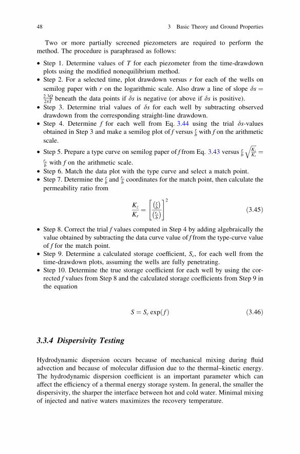
Two or more partially screened piezometers are required to perform themethod. The procedure is paraphrased as follows:

• Step 1. Determine values of T for each piezometer from the time-drawdownplots using the modified nonequilibrium method.

• Step 2. For a selected time, plot drawdown versus r for each of the wells onsemilog paper with r on the logarithmic scale. Also draw a line of slope ds ¼2:3Q2pT beneath the data points if ds is negative (or above if ds is positive).

• Step 3. Determine trial values of ds for each well by subtracting observeddrawdown from the corresponding straight-line drawdown.

• Step 4. Determine f for each well from Eq. 3.44 using the trial ds-valuesobtained in Step 3 and make a semilog plot of f versus r

b with f on the arithmeticscale.

• Step 5. Prepare a type curve on semilog paper of f from Eq. 3.43 versus rb

ffiffiffiffiKz

Kr

q¼

rcb with f on the arithmetic scale.

• Step 6. Match the data plot with the type curve and select a match point.• Step 7. Determine the r

b and rcb coordinates for the match point, then calculate the

permeability ratio from

Kz

Kr¼

rb

� �

rcb

� �

" #2

ð3:45Þ

• Step 8. Correct the trial f values computed in Step 4 by adding algebraically thevalue obtained by subtracting the data curve value of f from the type-curve valueof f for the match point.

• Step 9. Determine a calculated storage coefficient, Sc, for each well from thetime-drawdown plots, assuming the wells are fully penetrating.

• Step 10. Determine the true storage coefficient for each well by using the cor-rected f values from Step 8 and the calculated storage coefficients from Step 9 inthe equation

S ¼ Sc exp fð Þ ð3:46Þ

3.3.4 Dispersivity Testing

Hydrodynamic dispersion occurs because of mechanical mixing during fluidadvection and because of molecular diffusion due to the thermal–kinetic energy.The hydrodynamic dispersion coefficient is an important parameter which canaffect the efficiency of a thermal energy storage system. In general, the smaller thedispersivity, the sharper the interface between hot and cold water. Minimal mixingof injected and native waters maximizes the recovery temperature.


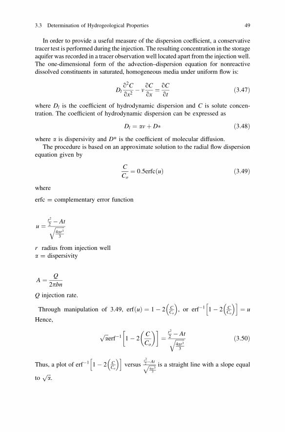
In order to provide a useful measure of the dispersion coefficient, a conservativetracer test is performed during the injection. The resulting concentration in the storageaquifer was recorded in a tracer observation well located apart from the injection well.The one-dimensional form of the advection–dispersion equation for nonreactivedissolved constituents in saturated, homogeneous media under uniform flow is:

Dlo2C

ox2� v

oC

ox¼ oC

otð3:47Þ

where Dl is the coefficient of hydrodynamic dispersion and C is solute concen-tration. The coefficient of hydrodynamic dispersion can be expressed as

Dl ¼ avþ D� ð3:48Þ

where a is dispersivity and D* is the coefficient of molecular diffusion.The procedure is based on an approximate solution to the radial flow dispersion

equation given by

C

Co¼ 0:5erfc uð Þ ð3:49Þ

where

erfc = complementary error function

u ¼r2

2 � Atffiffiffiffiffiffiffi4ar3

3

q

r radius from injection wella = dispersivity

A ¼ Q

2pbn

Q injection rate.

Through manipulation of 3.49, erf uð Þ ¼ 1� 2 CCo

� �, or erf�1 1� 2 C

Co

� �h i¼ u

Hence,

ffiffiffiap

erf�1 1� 2C

Co

� �� ¼

r2

2 � Atffiffiffiffiffiffiffi4ar3

3

q ð3:50Þ

Thus, a plot of erf�1 1� 2 CCo

� �h iversus

r22�Atffiffiffiffiffi

4ar33

p is a straight line with a slope equal

toffiffiffiap

.


3.4 Determination of Thermal Properties

The major thermodynamic quantities which must be measured or at least estimatedare the thermal conductivity and heat capacity of the aquifer and confining layers.These quantities are subject to much less natural variation than the hydraulicproperties which were discussed previously. Therefore, they can normally beestimated or measured in the laboratory using core samples obtained duringconstruction of the various exploratory and/or test wells.

The specific heats of many common dry rock materials are in the relativelynarrow range of 0.19–0.22 kcal/kg/�C. Using values for pure materials obtainablefrom standard tables, one can estimate the effective heat capacity of a watersaturated porous medium on a volumetric basis using the equation

Cva ¼ nqwCw þ 1� nð ÞqsCs ð3:51Þ

where Cva aquifer volumetric heat capacity; qw, qs densities of water and solidrespectively; Cw, Cs specific heat of water and solid respectively; and n porosity. Aporosity in the range of 20–60 % would yield an effective heat capacity betweenabout 600 and 800 kcal/m3/�C.

The knowledge of underground thermal properties is a prerequisite for properdesign of borehole heat exchangers (BHE). The most important property is thethermal conductivity of the ground. This parameter is site specific and cannot beinfluenced by engineering. The thermal contact from the borehole wall to the fluidinside the pipes, however, is controlled by borehole diameter, pipe size and con-figuration, pipe material, and the filling inside the annulus. These items are subjectto efforts in order to reduce the thermal resistance between borehole wall and fluid,usually summarized in the parameter ‘‘borehole thermal resistance’’.

Since the mid 1990s, a method has been developed and refined to measure theunderground thermal properties on-site, and mobile equipment for these mea-surements has been built in several countries. The TRT, also sometimes calledgeothermal response test (GRT), is a suitable method to determine the effectivethermal conductivity of the underground and the borehole thermal resistance or thethermal conductivity of the borehole filling, respectively (Sanner et al. 2005).From the test, a temperature curve is obtained which can be evaluated by differentmethods. The resulting thermal conductivity is a value for the total heat transportin the underground, noted as a thermal conductivity. Other effects like convectiveheat transport (in permeable layers with groundwater) and further disturbances areautomatically included, so it may be more correct to speak of an ‘‘effective’’thermal conductivity keff .


3.4.1 Development of Thermal Response Test

The theoretical basis for the TRT was laid over several decades. In the 1990s, thefirst practical applications were made, e.g., for the investigation of borehole heatstorage in Linköping. In 1995, a mobile test equipment was developed at LuleåTechnical University to measure the ground thermal properties for BHE betweensome 10 m to over 100 m depth. A similar development was going on indepen-dently since 1996 at Oklahoma State University in the U.S.A. The first TRT inGermany was performed in summer 1999 (Sanner et al. 2005).

A somewhat different test rig was developed and tested in the Netherlands. Thisrig uses a heat pump instead of electric resistance heaters, in order to be able toalso decrease the temperature inside the BHE. This method, however, has intrinsicproblems because of the dynamic behavior of the heat pump and the need for aheat source/sink, and should only be used where testing with extracting heat has tobe done explicitly. Besides the Dutch test rig, there are at least two other heatpump systems, one in Germany and one in Sweden.

There are test rigs operational today in the following countries:

• Canada• Chile (experimental)• China• Germany (4)• Netherlands• Norway• South Korea• Sweden (several)• Switzerland• Turkey• United Kingdom• U.S.A. (several)

3.4.2 Operation of the Test

The general layout of a TRT is shown in Fig. 3.9. For good results, it is crucial toset up the system correctly and to minimize external influences. This is done easierwith heating the ground (electric resistance heaters) than with cooling (heatpumps). However, even with resistance heating, the fluctuations of voltage in thegrid may result in fluctuations of the thermal power injected into the ground.

Other sources of deviation include climatic influences, affecting mainly theconnecting pipes between test rig and BHE, the interior temperatures of the testrig, and sometimes the upper part of the BHE in the ground. Heavy insulation isrequired to protect the connecting pipes, and sometimes even air-conditioning for

3.4 Determination of Thermal Properties 51

the test rig is necessary, as was done in U.S.A. With open or poorly grouted BHE,also rainwater intrusion may cause temperature changes. A longer test durationallows for statistical correction of power fluctuations and climatic influence, andresults in more trustworthy evaluation. Typical test curves with strong and withlow climatic influence are shown in Fig. 3.10.

With the increasing commercial use of TRT, the desire for a shorter testduration became apparent, in particular in the U.S.A. A recommendation for aminimum of 50 h was given, which is compatible with the IEA recommendations,but there is also skepticism. A test time of about 12 h is desired, which also wouldallow not to have the test rig out on the site overnight, In general, there arephysical limits for the shortening of the measuring period, because a somewhatstable heat flow has to be achieved in the ground. In the first few hours, thetemperature development is mainly controlled by the borehole filling and not bythe surrounding soil or rock. A time of 48 h is considered by the authors as theminimum test period.

In the evaluations made of German tests, the minimum duration criterionproved helpful:

tb ¼5r2

að3:52Þ

with

tb lower time limit of data to be usedr borehole radius

a thermal diffusivity with estimated values a ¼ kqCp

� �

Fig. 3.9 Test setup for aThermal Response Test(redrawn from Sanner et al.2005)


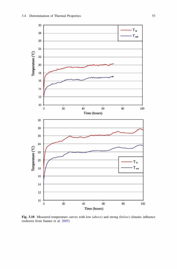
Fig. 3.10 Measured temperature curves with low (above) and strong (below) climatic influence(redrawn from Sanner et al. 2005)


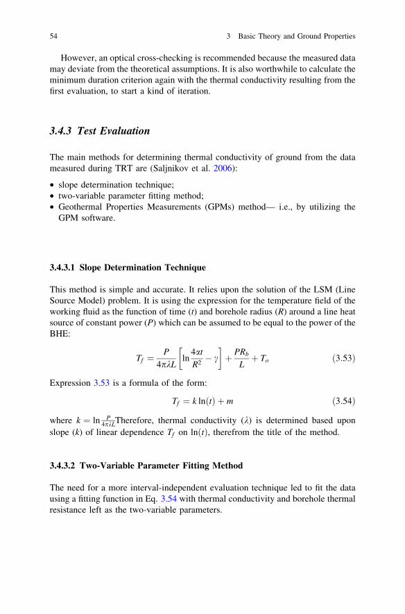
However, an optical cross-checking is recommended because the measured datamay deviate from the theoretical assumptions. It is also worthwhile to calculate theminimum duration criterion again with the thermal conductivity resulting from thefirst evaluation, to start a kind of iteration.

3.4.3 Test Evaluation

The main methods for determining thermal conductivity of ground from the datameasured during TRT are (Saljnikov et al. 2006):

• slope determination technique;• two-variable parameter fitting method;• Geothermal Properties Measurements (GPMs) method— i.e., by utilizing the

GPM software.

3.4.3.1 Slope Determination Technique

This method is simple and accurate. It relies upon the solution of the LSM (LineSource Model) problem. It is using the expression for the temperature field of theworking fluid as the function of time (t) and borehole radius (R) around a line heatsource of constant power (P) which can be assumed to be equal to the power of theBHE:

Tf ¼P

4pkLln

4at

R2� c

� �þ PRb

Lþ To ð3:53Þ

Expression 3.53 is a formula of the form:

Tf ¼ k ln tð Þ þ m ð3:54Þ

where k ¼ ln P4pkLTherefore, thermal conductivity (k) is determined based upon

slope (k) of linear dependence Tf on ln tð Þ, therefrom the title of the method.

3.4.3.2 Two-Variable Parameter Fitting Method

The need for a more interval-independent evaluation technique led to fit the datausing a fitting function in Eq. 3.54 with thermal conductivity and borehole thermalresistance left as the two-variable parameters.


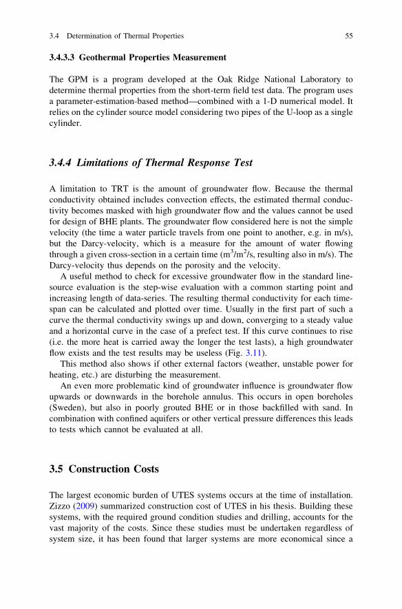
3.4.3.3 Geothermal Properties Measurement

The GPM is a program developed at the Oak Ridge National Laboratory todetermine thermal properties from the short-term field test data. The program usesa parameter-estimation-based method—combined with a 1-D numerical model. Itrelies on the cylinder source model considering two pipes of the U-loop as a singlecylinder.

3.4.4 Limitations of Thermal Response Test

A limitation to TRT is the amount of groundwater flow. Because the thermalconductivity obtained includes convection effects, the estimated thermal conduc-tivity becomes masked with high groundwater flow and the values cannot be usedfor design of BHE plants. The groundwater flow considered here is not the simplevelocity (the time a water particle travels from one point to another, e.g. in m/s),but the Darcy-velocity, which is a measure for the amount of water flowingthrough a given cross-section in a certain time (m3/m2/s, resulting also in m/s). TheDarcy-velocity thus depends on the porosity and the velocity.

A useful method to check for excessive groundwater flow in the standard line-source evaluation is the step-wise evaluation with a common starting point andincreasing length of data-series. The resulting thermal conductivity for each time-span can be calculated and plotted over time. Usually in the first part of such acurve the thermal conductivity swings up and down, converging to a steady valueand a horizontal curve in the case of a prefect test. If this curve continues to rise(i.e. the more heat is carried away the longer the test lasts), a high groundwaterflow exists and the test results may be useless (Fig. 3.11).

This method also shows if other external factors (weather, unstable power forheating, etc.) are disturbing the measurement.

An even more problematic kind of groundwater influence is groundwater flowupwards or downwards in the borehole annulus. This occurs in open boreholes(Sweden), but also in poorly grouted BHE or in those backfilled with sand. Incombination with confined aquifers or other vertical pressure differences this leadsto tests which cannot be evaluated at all.

3.5 Construction Costs

The largest economic burden of UTES systems occurs at the time of installation.Zizzo (2009) summarized construction cost of UTES in his thesis. Building thesesystems, with the required ground condition studies and drilling, accounts for thevast majority of the costs. Since these studies must be undertaken regardless ofsystem size, it has been found that larger systems are more economical since a


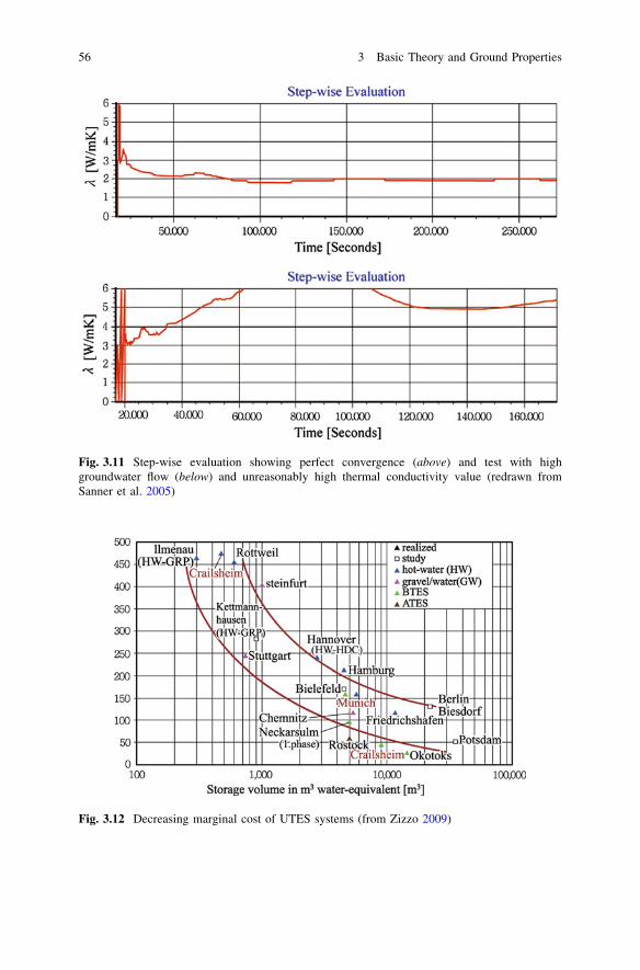
Fig. 3.11 Step-wise evaluation showing perfect convergence (above) and test with highgroundwater flow (below) and unreasonably high thermal conductivity value (redrawn fromSanner et al. 2005)

Fig. 3.12 Decreasing marginal cost of UTES systems (from Zizzo 2009)


greater output is achieved for marginally increased capital expenditures. Figure 3.12illustrates that as system size increases, the investment per unit output decreases.

Nordell and Hellström (2000) performed a detailed energy simulation for asolar heated BTES system. The system was designed to serve 90 building units of100 m2 each using a 3,000 m2 roof-mounted solar collection system and a 99borehole BTES system of 65 m depth for a storage volume of 60,000 m3. It wasestimated that 60 % of the total heat demand would be met by the system. Theconstruction cost, including heat exchanger installations in buildings (which canrange from $1,000 to $10,000), and annual operation expenses were then com-pared with two conventional alternate systems—a small-scale, biomass pellet andoil DE system, and a GSHP system for each building. A summary of his findingscan be seen in Table 3.3, showing that the DE system has the lowest constructioncost, but also the highest annual cost. The solar heated BTES has the highest initialcost, but has an annual cost only 8 % higher than the least expensive annual optionof GSHP (annual DE costs are 20 % above GSHP). This example illustrates thatalthough UTES systems do cost more than some alternatives, they provide long-term stability of energy pricing into the future and should be considered for futureprojects.

References

American Society for Testing and Materials (1999) Standard guide for selection of aquifer testmethod in determining hydraulic properties by well techniques, Annual book of ASTMstandards, West Conshohocken

Boonstra J (1999a) Well design and construction. In: Delleur JW (ed) The handbook ofgroundwater engineering. CRC Press, Boca Raton

Boonstra J (1999b) Well hydraulics and aquifer tests. In: Delleur JW (ed) The handbook ofgroundwater engineering. CRC Press, Boca Raton

De Smedt F (1999) Two- and three-dimensional flow of groundwater. In: Delleur JW (ed) Thehandbook of groundwater engineering. CRC Press, Boca Raton

Deng Z (2004) Modeling of standing column wells in ground source heat pump systems. Ph.D.Dissertation, Oklahoma State University, Stillwater, OK, USA


Fetter CW (2001) Applied hydrogeology, 4th edn. Prentice Hall, Upper Saddle RiverHall SH, Raymond JR (1992) Geohydrologic characterization for aquifer thermal energy storage.

In: 1992 intersociety energy conversion engineer conference, San Diego, CA, Aug 3–7, 1992http://capp.water.usgs.gov/GIP/gw_gip/how_occurs.html

Table 3.3 Solar heated BTES cost comparison with alternate systems (from Zizzo 2009)

System Construction costs(millions $ CAD)

Annual costs(millions $ CAD)

Solar heated BTES 1.377 0.161Small-scale DE 0.878 0.179GSHP for each building 0.945 0.149

3.5 Construction Costs 57


Jacob CE (1947) Drawdown test to determine effective radius of artesian well. Trans ASCE112:1047–1064

Lee SL, Yang JH (1998) Modelling of effective thermal conductivity for a nonhomogeneousanisotropic porous medium. Int J Heat Mass Transf 41(6–7):931–937

Nordell BO, Hellström G (2000) High temperature solar heated seasonal storage system for lowtemperature heating of buildings. Sol Energy 69(6):511–523

Parr AD, Molz FJ, Melville JG (1983) Field determination of aquifer thermal energy storageparameters. Groundwater 21(1):22–35

Sanner B, Hellström G, Spitler J, Gehlin S (2005) Thermal response test—current status andworld-wide application. In: Proceedings world geothermal congress 2005, Antalya, Turkey,April 24–29, 2005

Saljnikov A, Goricanec D, Kozic D, Krope J, Stipic R (2006) Borehole and aquifer thermalenergy storage and choice of thermal response test method. In: Proceedings of the 4thWSEAS international conference on heat transfer, thermal engineering and environment,Elounda, Greece, Aug 21–23, 2006, pp 11–15

Weeks EP (1969) Determining the ratio of horizontal to vertical permeability by aquifer testanalysis. Water Resour Res 14(1):196–214

Zizzo R (2009) Designing an optimal urban community mix for an aquifer thermal energy storagesystem. M.S. Thesis, University of Toronto, Toronto, Canada


Chapter 4Aquifer Thermal Energy Storage

4.1 Definition

In general, groundwater temperatures remain relatively stable at temperaturestypically 1–2 �C higher than local mean annual temperatures between depths of10–20 m. Below these depths, groundwater temperatures gradually increase at arate of geothermal gradient. As a result, in areas where a supply of groundwater isreadily available from an aquifer, a reliable source of low temperature geothermalenergy exists.

Open-loop geothermal systems use this resource by extracting groundwaterfrom an aquifer using a water well, and passing it across a heat exchanger toallow transfer of energy for direct use in the HVAC system of a building,typically in combination with a heat pump. The majority of open-loop systemssubsequently dispose of the used groundwater either by discharging to a surfacewater body or reinjecting into the aquifer. These types of open-loop systems,known as pump-and-release or pump-and-dump systems, are relatively simple toimplement. For commercial or institutional applications, they offer energy effi-ciencies comparable to closed-loop systems at substantially reduced capital costs(Bridger and Allen 2005).

In the open-loop systems, energy is typically transferred to and from thebuilding’s heating and cooling system via a heat exchanger. Conversely, closed-loop systems exchange energy directly in the ground using ground heat exchanges,which are commonly installed in adapted trenches at relatively shallow depth or invertical boreholes. Other variations allow for the transfer of energy through heatexchanger pipe work installed in foundation structures (Dickinson et al. 2009).

It is useful to understand a difference between higher and lower enthalpysystems. Higher enthalpy systems take advantage of higher temperature geother-mal resource generated from a heat flux originating from decaying radioactiveisotopes of uranium, potassium, and thorium in the deeper formation of the earth’scrust. Lower enthalpy systems utilize the net solar energy absorbed and stored inthe subsurface. In the lower enthalpy systems, the groundwater temperature near


59

the surface is inherently associated to the surface temperatures throughout theyear. There are seasonal fluctuations in temperatures within a few meters belowground surface. This effect is reduced with greater depth, so the prevailing tem-perature gradient relating to the thermal flux.

Open-loop systems are a particular type of low temperature geothermal system.A particular type of open-loop system using aquifers for energy storage, is referred asaquifer thermal energy storage (ATES) systems. Aquifer thermal energy storage is anapproach used to enhance the efficiency in comparison with other ground energysystem. ATES installation actively store cooled and heated groundwater in theground from respective heating and cooling mode cycles (Dickinson et al. 2009).

Goundwater is used to transfer the thermal energy into and out of an aquifer inATES systems. ATES systems utilize aquifers for the storage of low-grade thermalenergy such as solar heat or waste heat during off-peak periods. The low-gradeenergy is used to heat or chill water which is injected into an aquifer for storage.Later, the water is withdrawn for space heating or cooling during a period of highdemand.

Water wells are used for the connection to the aquifer. However, these wells arenormally designed with double functions, both as production and infiltration wells,as shown in Fig. 4.1 (Andersson 2007). The energy is partly stored in thegroundwater itself but partly also in the grains (or rocks mass) forming the aquifer.The storage process in the rocks mass takes place when the groundwater is passingthe grains and will lead to the development of a thermal front with differenttemperatures. This front will move in a radial direction from the well duringcharging of the store and then turn back during discharging.

Practically all systems are designed for low temperature applications whereboth heat and cold are seasonally stored. However, the systems are sometimes alsoapplied for short-term storage.

ATES open-loop systems can offer increased energy efficiency and long-termcost savings over pump and dump systems and closed-loop systems by using anaquifer as a seasonal storage reservoir for waste or excess thermal energy gen-erated in off-peak seasons or periods of low demand such as solar energy insummer months or cold air in winter months. ATES systems are operated bytransferring heat or cold mass to or from groundwater through a heat exchanger.The groundwater that is injected back into the aquifer is heated or chilled. Thereinjected groundwater may hold a temperature higher or lower than the undis-turbed ground temperature, depending on the thermal properties of the ground andflow characteristics of the aquifer. During periods of high heating or coolingdemand, water is pumped from the aquifer and used as an energy source or sink.

60 4 Aquifer Thermal Energy Storage

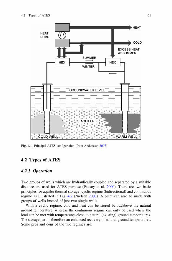
4.2 Types of ATES

4.2.1 Operation

Two groups of wells which are hydraulically coupled and separated by a suitabledistance are used for ATES purpose (Paksoy et al. 2000). There are two basicprinciples for aquifer thermal storage: cyclic regime (bidirectional) and continuousregime as illustrated in Fig. 4.2 (Nielsen 2003). A plant can also be made withgroups of wells instead of just two single wells.

With a cyclic regime, cold and heat can be stored below/above the naturalground temperature, whereas the continuous regime can only be used where theload can be met with temperatures close to natural (existing) ground temperatures.The storage part is therefore an enhanced recovery of natural ground temperatures.Some pros and cons of the two regimes are:

Fig. 4.1 Principal ATES configuration (from Andersson 2007)

4.2 Types of ATES 61

• Cyclic flow will create a definite cold and heat reservoir around each well orgroup of wells. Cold can be stored around one of the well groups heat can bestored and around the other. Groundwater is pumped from one of the wellgroups, and then heated or cooled within the building before being injected backinto the aquifer in the other well group. The groundwater circuit is closed in thesense that the water is produced from a number of warm wells and then injectedthrough the cold wells at the same flow rate and without being exposed to air. Itis possible to maintain a ground volume above or below the natural groundtemperature all the time. One disadvantage is a more complicated well designand control system with each well being able to both produce and injectgroundwater.

• Continuous flow is simpler with regard to system design and well control, andonly one well or group of well need to be equipped with pumps. The disad-vantage is the limited temperature range.

Summer

warm well cold well

aquifer

Winter

warm well cold well

aquifer

Summer

aquifer

heatmean temperature

Winter

mean temperature cold

aquifer

(a)

(b)

Fig. 4.2 Basic operational regimes for aquifer thermal energy storage (a) continuous regime,(b) cyclic regime (from Nielsen 2003)


4.2.2 Form of Energy

On the basis of the form of energy being stored, three main types of ATES systemscan be defined. These are chilled water storage systems (or cold storage), heatstorage systems, and integrated heat and cold storage systems.

Cold storage involves the injection, storage, and recovery of chilled (or cold)water at temperatures between 6 and 12 �C in a suitable storage aquifer for storageperiods from several hours to several months. One or more wells are useddepending on energy requirements and the properties of the aquifer.

Applications of cold storage include primarily air conditioning and equipmentcooling in institutional and commercial buildings, and industrial process cooling.These systems are best applied when a demand for cooling exists for significantportion of the year. Presently, many cold storage systems operate in Europe andNorth America, particularly in The Netherlands. The storage efficiency of a coldstorage system is equivalent to the amount of energy injected into an aquifer (e.g.,energy injected to the aquifer while cooling a building) divided by the amount ofenergy taken from an aquifer (e.g., energy rejected from the aquifer using a fluidcooler to passively refrigerate the aquifer during cold spells). It should be calcu-lated over an entire charge/discharge cycle where the aquifer reaches the samebulk temperature at the end of each cycle, which is ideal for environmental sus-tainability considerations. It can reach 70–100 % for most long-term cold storageprojects. The cold storage efficiency decreases as the heat transfer from the sur-roundings to the storage aquifer increases.

Heat storage involves the injection, storage, and recovery of heated water in asuitable storage aquifer. Heat storage systems can be classified on the basis of lowto moderate temperature heat (10–40 �C) or high temperature heat (40–150 �C).The components, well configurations, and storage periods of heat storage ATESsystems are similar to cold storage systems. Applications of aquifer heat storageexist in space heating, industrial heating, heating for agricultural purposes (e.g.,greenhouses), and roadway de-icing and snow-melting. Because convective heatlosses (buoyancy effects) are greater for heat storage than for cold storage, thestorage efficiency is typically less than that of cold storage and ranges from 50 to80 %.

To counter the effects of higher heat losses due to convection currents, thestorage wells for high temperature heat storage are preferably drilled to greaterdepths. This minimizes heat losses by using the overburden formation above thestorage aquifer as an insulator between the warm aquifer and the cooler ambientair, and by choosing a storage medium that is surrounded by warmer materials dueto the geothermal gradient, thereby reducing losses.

Integrated or combined heat and cold ATES systems may offer an improvedefficiency over cold- or heat-only storage systems, particularly in large-scaleapplications. These systems are most commonly used in combination with a heatpump to provide heating and cooling in commercial or institutional buildings.

4.2 Types of ATES 63

The components of combined systems are virtually the same as for cold orwarm mass storage alone. However, the design of above-ground and below-groundcomponents of integrated systems is more complicated. For underground com-ponents, the positioning of the wells become more important as the aquifer is usedas a heat source or sink. Specifically, storage of warm and cold mass results in thedevelopment of thermal plumes around the wells and there is increased risk of heattransfer between them.

From an economic perspective, integrated ATES systems for combined spaceheating/cooling applications using a heat pump, with no other sources of wasteheat or chilled water, may be more sensitive to costs associated with aquifercharacterization and other design costs compared to ATES systems with highergrade waste heat sources. In smaller applications, it will be challenging to rely on arelatively small increase in heat pump coefficient of performance (COP) to gen-erate sufficiently attractive returns on the incremental capital investment. Theincreased complexity of the system, in addition to the effort for aquifer charac-terization, may add significant cost to the project. In the cooling mode applicationof an integrated ATES system, an opportunity may exist for direct cooling(without the use of a heat pump) where direct cooling might otherwise not bepossible. In this case, substantial energy savings could result.

COP is the classic parameter that has been used to describe the performance ofa heat pump. A simple definition of the coefficient of performance adequate for ourpurposes is The COP is a dimensionless parameter on which upper bounds can befound using the laws of thermodynamics. It is common in the U.S. air-conditioningindustry to report the cooling performance in terms of what is called the ‘‘energyefficiency ratio’’ or EER. The EER is not a dimensionless parameter, as the energyinput rate is in watts and the output thermal effect is in Btu/h. The EER can bereadily determined by multiplying the COP by 3.413. While COPs will vary,depending on the quality of the heat pump unit and its operating conditions, in theheating mode, COPs in the range of 3–4.5 can be expected for GSHPs. In thecooling mode, performance will generally be lower; a net COP of 2–3.5 can beexpected when the heat load within the conditioned space that is generated by thefans, compressors, and parasitics is subtracted from the gross cooling effect. Whencomparing GSHP system performance to conventional system performance thedesigner must be careful to also include all the parasitic losses of the conventionalsystems if a legitimate comparison is to be achieved (Phetteplace 2007).

4.3 Aquifer and Groundwater

4.3.1 Aquifer

To be able to construct an ATES systems a suitable aquifer has to at hand at orclose to the site where the ATES user is located. As explained in Chap. 2,‘‘aquifer’’ is defined as a geologic formation that contains sufficient saturated


http://dx.doi.org/10.1007/978-1-4471-4273-7_2

permeable material to yield economical quantities of water to wells and springs.An aquifer is in practice defined to be a geological formation from whichgroundwater can be pumped by using water wells.

Groundwater refers to subsurface water found beneath the water table in thevoid spaces of unconsolidated (i.e., sands and gravels) and consolidated (i.e.,sandstone and volcanic rocks) geologic formations. A groundwater aquifer existsin geologic formations which are sufficiently permeable to store and yield largequantities of groundwater.

By definition groundwater can be found almost anywhere. The groundwatertable is defined as the level under which all pores or fractures are water saturated.Above the water table lies the unsaturated zone, where voids between rocks aremostly filled with air. Some water is held in the unsaturated zone by molecularattraction, and it will not flow toward or enter a well. In the saturated zone, whichlies below the water table, all the openings in the rocks are full of water that maymove through the aquifer to streams, springs, or wells from which water is beingwithdrawn.

There are two major types of aquifers. If the groundwater stands in directcontact with the atmosphere, the aquifer is regarded as unconfined. If, on the otherhand a permeable formation below the groundwater table is covered by a lesspermeable layer, the aquifer is regarded as confined.

The confined type of aquifer has a hydraulic pressure (static head) that is on ahigher level than the top of the aquifer. This artesian pressure can sometimes reachabove the surface level resulting in self-flowing wells or artesian wells. In nature,the groundwater is a part of the hydrological cycle. Hence, groundwater is natu-rally recharged and drained. Sometimes the draining is shown up as springs, butmore common it flows out to a lake or a river.

4.3.2 Aquifer Properties

To determine the suitability of an aquifer for thermal energy storage, a charac-terization of the aquifer must be performed. Aquifer characterization for an ATESproject usually involves a detailed assessment of the aquifer in terms of itsgeology, physical properties, flow characteristics, and water chemistry. Thesecharacteristics are similar to those assessed for most environmental investigationsor water supply studies.

Any ATES application will require a good knowledge on the properties of theaquifer being the target to use (Andersson 2007). The most important propertiesfor ATES application include geometry (surface area and thickness), stratigraphy(different layers of strata), static head (groundwater or pressure level), ground-water table gradient (natural flow direction), hydraulic conductivity (permeability),transmissivity (hydraulic conductivity 9 thickness), storage coefficient (yield as afunction of volume), leakage factor (vertical leakage to the aquifer), and boundaryconditions (surrounding limits, positive or negative). The first four items are

4.3 Aquifer and Groundwater 65

studied by using topographical, geological and hydrogeological maps anddescriptions, data from existing wells and older site investigations. The latter onesmay contain geophysical data as well as pumping tests and so forth. Any infor-mation on groundwater chemistry is of importance as well as information of thenatural groundwater temperature (Bridger and Allen 2005)

4.3.2.1 Geology and Aquifer Thickness

The physical makeup of the sediments or rocks and depth, aerial extent, andthickness of permeable and impermeable geological units both at a regional scaleand locally at the proposed ATES site, are important factors in determining thenature and distribution of aquifers in the subsurface. The majority of thermalstorage projects use unconsolidated aquifers as storage media. However, unfrac-tured and highly fractured bedrock aquifers also can be used for thermal energystorage. In these aquifers, the mapping of structural features, such as fractures andfaults that strongly influence fluid flow, will be also important.

4.3.2.2 Hydraulic Properties and Groundwater Flow

The effective porosity and the hydraulic properties such as hydraulic conductivityand specific storage are important to the design and evaluation of ATES systems.The effective porosity refers to the system of interconnected void space in theporous aquifer media. It is important in determining the amount of heated orchilled water that can be stored per unit volume of the aquifer.

The hydraulic conductivity is a measure of the ability of the porous medium totransmit water. High hydraulic conductivities are required for large flow rates ofwater to be withdrawn or injected from or to the aquifer with the least change tothe hydraulic and temperature gradients around the production wells. Specificstorage is a measure of the water storage capacity of an aquifer and is defined asthe volume of water that a unit volume of aquifer releases from storage under aunit decline in hydraulic head. These properties, along with the hydraulic gradient,control the velocity, and direction of groundwater flow or the flow regime in anaquifer.

4.3.2.3 Thermal Properties and Ground Temperature Field

The physical processes of conduction and convection govern the transport andstorage of heat in an aquifer. Conductive heat transport refers to the movement ofheat along a thermal gradient. Convective heat transport refers to the movement ofheat by flowing groundwater. In an ATES system, conductive heat transport occursdue to the temperature gradients induced by warmer or cooler storage watercoming into contact with the surrounding aquifer water. The conduction of heat in


the aquifer is governed by the thermal properties of aquifer such as the volumetricheat capacity and the effective thermal conductivity. Heat capacity indicates theamount of temperature change that occurs when the aquifer media absorbs or losesa specific amount of energy and thermal conductivity represents the ability of theaquifer media to transmit heat. Since water has a higher heat capacity but lowerthermal conductivity than rock, the storage of thermal energy in aquifers is bestsuited to a high porosity formation to minimize conductive energy losses andincrease the efficiency of the thermal store.

Convective heat transport results from groundwater flow driven by hydraulichead and temperature differentials, which exist both locally in the vicinity of thewell field as a result of pumping/injection of groundwater and regionally within theaquifer. Convective heat transport has both advective and dispersive components.

Advection describes the movement of thermal energy directly due to theaverage linear flow of groundwater through the porous medium. Thermal disper-sion refers to the microscopic dispersal or spreading of thermal energy in threedimensions beyond the regions it normally would occupy as a result of advectionalone. Dispersion can be regarded as a zone of mixing, which travels in advance ofthe thermal energy front defined by advection. In addition, free convection alsooccurs when groundwater movement is driven by density variations due totemperature gradients. In high temperature ATES systems, the effects of freeconvection will become important, as the thermal energy will rise due to a lowereddensity of the heated water. In lower temperature ATES systems, including heatstorage and cold storage, the density differences between the stored water and theambient groundwater will be small enough so that free convection is limited.

Regional groundwater flow is an important consideration in the design of ATESsystems as higher groundwater flow regimes can lead to advection or down-gradient ‘drift’ of stored energy beyond potential recovery regions. In the presenceof a steep regional gradient in hydraulic head, which would correspond to fastergroundwater flows, a lower permeability aquifer is required to minimize convec-tive losses (dispersion reduces the thermal intensity of the recovered plume). Inaddition, small-scale vertical and horizontal variations in hydraulic conductivity orheterogeneity in the aquifer that result from changes in geology are important, asthese will affect the dispersion of the thermal plume.

4.3.2.4 Groundwater Chemistry

The chemistry of aquifers often represents a significant problem in the design ofATES systems. The primary problems related to groundwater chemistry include(1) the scaling of heat exchangers and clogging of wells resulting from the pre-cipitation of minerals such as calcium carbonate and iron or manganese oxides, (2)the corrosion of piping and heat exchangers by ambient and heated groundwater,(3) biofouling of the well intake area; and (4) the clogging of the aquifer as a resultof precipitation of minerals within the aquifer or the transport of precipitates intothe aquifer.


These problems are avoidable if consideration of the potential for geochemistryproblems is considered in advance of the system design phase. Many designstrategies and water treatment technologies have been used to mitigate theseproblems.

4.3.3 Aquifer Characterization

Aquifer characterization for an ATES project typically involves phases of desktopreview, drilling, hydraulic testing, and modeling, although the level of complexityof these characterization steps can vary considerably depending on how muchinformation is known about the local geology/hydrogeology and how large theATES system will be.

A simple review can be performed as a preliminary data gathering or prefea-sibility study step to determine whether an ATES system is feasible. If the area iswell developed and much is known already about the hydrogeology of the area,then geological/hydrogeological investigative costs can be kept to a minimum. Inunexplored areas, more effort may be needed.

In a prefeasibility study, information regarding the site geology and ground-water potential often can be obtained from various sources such as existing nearbywater wells, previous hydrogeological investigations, aerial photographs, topo-graphic and geologic maps. If there is a suitable aquifer being capable of yieldingthe amount of water required for the project, one need to determine the number ofwells needed to meet the demand, bearing in mind peak demand, average demand,and the fact that injection wells are often less efficient at receiving water.Ultimately, a well (or wells) will have to be hydraulically tested to ensure that theyare capable of producing and receiving water. The spacing of the wells only can beestimated by a hydrogeologist in a preliminary sense. A decision then can be madeconcerning space availability, piping costs, etc.

If the prefeasibility study suggests that ATES is feasible, then a preliminary testwell should be drilled to confirm the information collected to that point. It is notrecommended that an expensive production size well be drilled initially, particu-larly if large diameter wells are needed. A test well can later be over-drilled to aproduction diameter. Logging of borehole cuttings/sediments should be under-taken to verify the geology, and identify permeable zones and target aquifers. Inunconsolidated aquifers, grain size analyses should be performed on these sedi-ments to select an appropriate slot size for a well screen. Sampling and analysis ofgroundwater should be carried out to assess groundwater chemistry.

To determine the hydraulic properties of the aquifer, and to assess the responseof the aquifer to pumping and injection during operation of the ATES system,hydraulic testing of the aquifer should follow test drilling. Constant dischargepumping tests, step-injection tests, step-drawdown tests, and tracer tests areexamples of tests performed for ATES aquifer characterization, although not all ofthese need to be done. Thermal conductivity can be calculated using values for


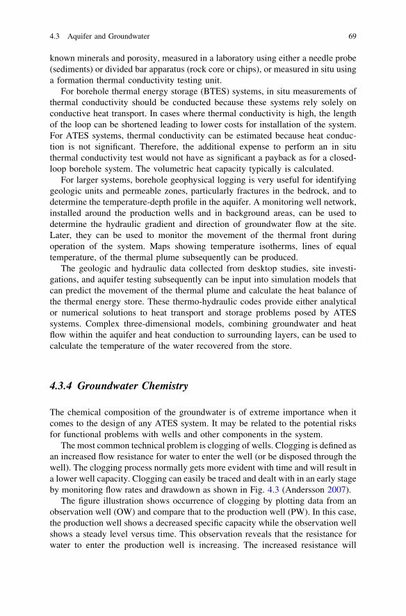
known minerals and porosity, measured in a laboratory using either a needle probe(sediments) or divided bar apparatus (rock core or chips), or measured in situ usinga formation thermal conductivity testing unit.

For borehole thermal energy storage (BTES) systems, in situ measurements ofthermal conductivity should be conducted because these systems rely solely onconductive heat transport. In cases where thermal conductivity is high, the lengthof the loop can be shortened leading to lower costs for installation of the system.For ATES systems, thermal conductivity can be estimated because heat conduc-tion is not significant. Therefore, the additional expense to perform an in situthermal conductivity test would not have as significant a payback as for a closed-loop borehole system. The volumetric heat capacity typically is calculated.

For larger systems, borehole geophysical logging is very useful for identifyinggeologic units and permeable zones, particularly fractures in the bedrock, and todetermine the temperature-depth profile in the aquifer. A monitoring well network,installed around the production wells and in background areas, can be used todetermine the hydraulic gradient and direction of groundwater flow at the site.Later, they can be used to monitor the movement of the thermal front duringoperation of the system. Maps showing temperature isotherms, lines of equaltemperature, of the thermal plume subsequently can be produced.

The geologic and hydraulic data collected from desktop studies, site investi-gations, and aquifer testing subsequently can be input into simulation models thatcan predict the movement of the thermal plume and calculate the heat balance ofthe thermal energy store. These thermo-hydraulic codes provide either analyticalor numerical solutions to heat transport and storage problems posed by ATESsystems. Complex three-dimensional models, combining groundwater and heatflow within the aquifer and heat conduction to surrounding layers, can be used tocalculate the temperature of the water recovered from the store.

4.3.4 Groundwater Chemistry

The chemical composition of the groundwater is of extreme importance when itcomes to the design of any ATES system. It may be related to the potential risksfor functional problems with wells and other components in the system.

The most common technical problem is clogging of wells. Clogging is defined asan increased flow resistance for water to enter the well (or be disposed through thewell). The clogging process normally gets more evident with time and will result ina lower well capacity. Clogging can easily be traced and dealt with in an early stageby monitoring flow rates and drawdown as shown in Fig. 4.3 (Andersson 2007).

The figure illustration shows occurrence of clogging by plotting data from anobservation well (OW) and compare that to the production well (PW). In this case,the production well shows a decreased specific capacity while the observation wellshows a steady level versus time. This observation reveals that the resistance forwater to enter the production well is increasing. The increased resistance will


lower the drawdown inside the well, while the groundwater table outside the wellis kept constant. This will increase the hydraulic gradient between the well and theaquifer and hence maintain a constant flow rate.

‘‘False clogging’’ sometimes occurs. Such events are either explained by ageneral lowering of the groundwater table or by failure of the submersible pumpscutting down the flow rate. However, by monitoring both the production wells andthe aquifer in observation wells or pipes such events can be excluded as a result ofclogging.

4.4 Problems of Aquifer Thermal Energy Storages

4.4.1 Clogging

Scaling is precipitation within the above-ground portion of an ATES system andclogging of wells, gravel pack, adjacent aquifer represents reduced aquifer per-meability caused by precipitation within the aquifer. Both are caused by chemicalprecipitates and has been frequently encountered in existing ATES systems,especially the precipitation of carbonates in the systems operating above 85 �C andFe and Mn oxides in low temperature (\40 �C) systems (Jenne et al. 1992).

Fig. 4.3 Detection of clogging by using a monitoring program in an early stage (from Andersson2007)


The precipitation of Fe and Mn oxides is caused by a change in water chem-istry. Precipitation of Fe III oxides can be induced by increasing either the redoxpotential (Eh) or the pH. As illustrated in the Fe stability field diagram shown inFig. 4.4, if either the Eh or pH of slightly reduced water (point A in the diagram) isincreased, precipitation of Fe oxides is likely. Not shown on this figure is the effectof Fe concentration; as Fe concentration increases, its oxide will precipitate atprogressively lower Eh and pH values. In practice, there are at least three processesinvolved to create the Eh and pH changes. Those are (1) oxygen is added fromsome source and the Eh value is increased (displacement from A to B in Fig. 4.4);(2) waters differing in their Eh status are mixed upon entering the well causingeither an increase or decrease in Eh and possibly pH (A to B or B to A); or (3)carbon dioxide escapes from the water, increasing the pH-value (A to C). The latterprocess is also believed to be one of the main factors causing the precipitation ofcarbonates in a well with little or no scaling in the heat exchanger. Where there aresignificant Fe concentrations, Fe carbonate rather than Ca carbonate may precip-itate. The Fe carbonate precipitate is not readily solubilized by acid treatment ofthe well.

Shallow, unconfined aquifers generally have levels of Fe and Mn that are likelyto yield oxyhydroxide precipitates if air is allowed to enter the ATES system. Anair leak in the ATES system caused Fe and Mn scaling of the well screen.

However, none of the processes causing Fe oxide precipitation need occurduring injection if the system is airtight, and the aquifer is selected or thehydrology is controlled to eliminate the mixing of dissimilar waters near the well.For these reasons, the likelihood of Fe oxide clogging during injection is low in aproperly designed system. If for any reason an airtight system is not feasible, anyone of a number of iron removal methods may be used.

Clogging by biofilm or microbial slime is a well-known phenomenon in thewater-well industry. The most frequent biologically caused well clogging is thatassociated with iron bacteria, especially the ones belonging to the Gallionellafamily. However, in a highly reduced environment, clogging can also be associ-ated with sulfur bacteria. In ATES applications, clogging by iron bacteria slimewill is a potential risk mainly in low-temperature systems (less than 25 �C) and inwaters with an iron content of at least 1 mg/L. Other conditions that favor majorbacterial growth are Eh values between 200 and 400 mV and pH values between5.5 and 7.5.

Gas clogging may occur as a result of the exsolution of gases present in excessof the amount that would be present at equilibrium with air at atmosphericpressure.

Swelling and dispersion of clays contained within the aquifer sediment occurswhen the Na saturation exceeds an amount determined by the ionic strength(i.e., conductivity) of the water. Clay swelling and dispersion are unlikely to pose aproblem in consolidated or silica-cemented aquifers even when the water is passedthrough a Na ion exchanger repetitively. Clay swelling and/or dispersion has beenavoided by treating the minimum fraction of the water necessary to preventcarbonate scaling; no scaling is observed at a calcite saturation indices of 0.6–0.7.

4.4 Problems of Aquifer Thermal Energy Storages 71

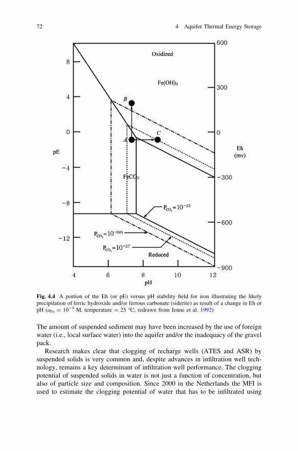
The amount of suspended sediment may have been increased by the use of foreignwater (i.e., local surface water) into the aquifer and/or the inadequacy of the gravelpack.

Research makes clear that clogging of recharge wells (ATES and ASR) bysuspended solids is very common and, despite advances in infiltration well tech-nology, remains a key determinant of infiltration well performance. The cloggingpotential of suspended solids in water is not just a function of concentration, butalso of particle size and composition. Since 2000 in the Netherlands the MFI isused to estimate the clogging potential of water that has to be infiltrated using

Fig. 4.4 A portion of the Eh (or pE) versus pH stability field for iron illustrating the likelyprecipitation of ferric hydroxide and/or ferrous carbonate (siderite) as result of a change in Eh orpH (aFe = 10-4 M, temperature = 25 �C; redrawn from Jenne et al. 1992)


recharge wells (Buik and Snijders 2006). The MFI gives no detailed informationabout each individual particle, instead it gives a direct value of the cloggingpotential of the water. In 2000, a quantitative relation between clogging rate andMFI was developed. In the years between 2000 and 2005, the relation was used todesign over 250 ATES systems. During these years the relation has proven itself asreliable and as a useful tool to predict clogging rates of recharge wells satisfactory,especially considering the uncertainties in measured parameters like MFI andpermeability. Further an easy, cheap (fast) and reliable apparatus was developed tomeasure the MFI of the water that has to be infiltrated.

Clogging caused by both straining and physical–chemical filtration can bedescribed by the following equation:

Dhv ¼1

qwg

� �cld

Kc

� �v2t ð4:1Þ

where Dhv = increment of pressure caused by clogging (mw); qw = density of theinfiltrated water (kg/m3); g = gravity acceleration (m/s2); c = concentration ofsuspended matter in the infiltration water (kg/m3); ld = dynamic viscosity (Ns/m2); Kc = intrinsic hydraulic conductivity of the filter cake on the borehole wall(m2); v = infiltration rate on the borehole wall (m/s); t = infiltration time (s).

One of the best parameters to predict the clogging potential of infiltration water,is the MFI. The MFI is a variation of the Silting Index (SI) and Silt Density Index(SDI). Both indices were developed to characterize the fouling potential of reverseosmosis feed water on RO membranes. The SI and the SDI have week theoreticalfoundations and do not vary linearly with the concentration of colloidal and sus-pended solids in water. The MFI, on the other hand, has a strong theoreticalfoundation and exhibits a linear correlation with the concentration of colloidal andsuspended solids in water.

The MFI is equal to the slope of the line that describes the inverse of the flowrate versus the amount of water that passes a membrane filter with 0.45 lm poresunder a constant pressure drop for standard conditions and can be described withEq. (4.2):

MFI ¼ ld

2pA2f

c

Kcð4:2Þ

where MFI = membrane filter index (s/l2); p = pressure loss (N/m2); Af = areaof the filter (m2).

If an MFI of 1 s/l2 is directly translated [with Eqs. (4.1 and 4.2)] into a cloggingrate for an infiltration well under standard conditions (Af ¼ 1:38� 10�3 m2 for astandard membrane filter; p = 2 9 105 Pa; ld ¼ 1:3� 10�3 Ns=m2 and v = 1 m/hon the borehole wall, a ‘common’ value for infiltration wells), the calculatedclogging rate of more than 2,000 m/y is not compatible with measured cloggingrates of around 0.1 m/y in the field. This demonstrates that a clogging rate derivedusing a filter with a pore size of 0.45 lm cannot be translated directly into a clogging


rate for an infiltration well. The calculated clogging rates were found to be morecompatible to clogging rates for water flood wells in oil fields. The difference wasattributed to the fact that the pore size of the receiving formation in an oil field iscloser to that of the MFI-membrane than the pore size in groundwater environments.

The MFI measured with a standard membrane filter can now be translated intoan MFI that is valid for other pore sizes.

MFIcor ¼ MFImea

Afp

Apð4:3Þ

where MFIcor = corrected MFI; MFImea = measured MFI; Afp = area of a pore ofthe applied filter; Ap = area of a pore for which the MFI must be corrected.

To calculate the ratio between the pore size of the aquifer and the pore size ofthe filter, it is necessary to estimate the pore size of the aquifer. The effective poresize is about a sixth of the median grain size of the sand (D50).

In an aquifer with a D50 of 300 lm the effective pore size is then about 50 lm.A measured MFI of 1 s/l2 (pore size 0.45 lm) will give a corrected MFI of8.1 9 10-5 s/l2 (Eq. 4.3). The calculated clogging rate (for an MFI of 1 s/l2 andv = 1 m/h) is now about 0.20 m/y, which is a realistic value.

Equations (4.1, 4.2 and 4.3) can be combined and rewritten as:

Dh

t¼

2MFImeapA2f

qwg

t

to

llo

Afp

Apv2 ð4:4Þ

The ratios tto

and llo

are added to make corrections for the amount of equivalent

full load hours per year (to ¼ 8; 760 h) and temperature influences (lo = viscosity

at 10 �C), and the ratio Afp

Apis added to translate a measured MFI to an MFI for the

aquifer.For practical use the D50 is translated into hydraulic conductivity K;

K ¼ 150 D50103� �1:65 ð4:5Þ

with D50 in m and K in m/d. Equation 4.5 can be rewritten as:

D50 ¼ 10�3 K

150

� �0:6

ð4:6Þ

If the standard circumstances for the MFI measurement are substituted in 4.5,the equation can be simplified and rewritten to (t is replaced by ueq and Dhv

t isreplaced by vv i.e. the clogging rate):

vv ¼ 2� 10�6 MFImeaueq

v2b

K150

� �1:2 ð4:7Þ


where ueq = amount of equivalent full load hours per year (h) (m3 infiltrated peryear divided by max. flow rate in (m3/h)); vv = clogging rate (mw/y);vb = infiltration rate on the borehole wall (m/h).

The water that is infiltrated will not be distributed equally over the height of theaquifer but it is divided over the well screen in relation to the hydraulic conduc-tivity of the aquifer. This means that layers with a high hydraulic conductivity arereceiving more water than layers with a low hydraulic conductivity. The infiltra-tion rate in layers with a high hydraulic conductivity is therefore higher than inlayers with a low hydraulic conductivity, and because the clogging rate is qua-dratically related to the infiltration rate (and linear to the MFI), these layers with ahigh hydraulic conductivity will clog faster than layers with a low hydraulicconductivity.

4.4.2 Corrosion

Both chemical and electrochemical corrosions may occur in ATES systems.Chemical corrosion is induced by constituents, such as CO2, O2, H2S, dissolvedsulfide, chloride, and sulfate. Corrosion was also experienced when a pipe con-nection was not sufficiently tight and allowed a small amount of air to diffuse throughthe threaded joint and react with reduced groundwater. Electrochemical corrosionappears to be more frequent than chemical corrosion. Electrochemical corrosion iscaused mainly by joining metals with different electrochemical potentials butelectrochemical corrosion also occurs on monometallic components that have beenstressed, e.g., welded joints, cut surfaces, or damaged coatings. Further, it seems thatelectrochemical corrosion causes loss of material only on parts of well screens andcasings. Usually it occurs in water that is slightly acidic and with total dissolvedsolids greater than about 1,000 mg/L.

Protection against corrosion is in most cases dependent upon the choice ofmaterials for each specific system. For instance, different steel alloys may copewith expected corrosion, as well as plastic materials, ceramics, or corrosion-resistant coatings. A world-wide method for galvanic corrosion protection of wellsis to use a cathodic protection system, normally accomplished by connecting asacrificial anode to the well casing.

4.4.3 Other Problems

Some of the problems and future issues with ATES may include:

• Interference between wells, especially between group of ‘‘warm’’ wells andgroup of ‘‘cold’’ wells. Detailed investigation, calculation, and simulation shouldbe conducted to establish the optimal well density, interval, and interactions


before the practical implementation. Some of simulation programs can be used topredict the spread of thermal fonts under different well plannings.

• Better combination of heat pump and ATES. It is better to find the optimal waysto combine heat pumps and ATES, because different combination methods willinfluence the design value of warm/cold well temperature and heating/coolingeffect of the whole system. Furthermore, it is very useful and significant toinvestigate the compatibility between ATES, heat pumps, and the whole dis-tribution system. Their individual viable and vulnerable features need to bechecked when the other components fail. For example, for the ATES heatingsystem in Rostock introduced in (Bauer et al. 2010), the failure of heat pumpslead directly to the poor performance of ATES after 2006. If this problem can besolved, ATES will be more desirable.

• Currently, very few researches are focusing on the environmental impact ofATES to the surrounding aquifer and soil layers, such as (1) influences of theincreased or decreased temperatures around the warm or cold wells on the localbiological communities, (2) influences of the varied temperatures on thechemistry composition and properties of the local aquifer water, and (3) influ-ences of the varied temperatures and the well operations on the geologicalstructures of the local soils. All these questions are lacking enough investiga-tions, simulations, research and references.

4.5 Construction of ATES

Construction of ATES is summarized by AEE Institute for Sustainable Technologies(2006). Aquifers are below-ground widely distributed and water filled permeableformations with high hydraulic conductivity, such as sand, gravel, sandstone, orlimestone layers. If there are impervious layers above and below and no or onlylimited natural groundwater flow, they can be used for thermal energy storage. Inthis case, two wells or groups of wells are drilled into the aquifer formation andserved for extraction or injection of groundwater. As seen in Fig. 4.5, coldgroundwater is extracted from the cold well during charging periods, heated up bythe heat source (e.g. solar or waste heat), and injected into the warm well. Indischarging-periods the flow direction is reversed. Warm water is extracted from thewarm well, cooled down by the heat sink, and injected into the cold well. Because ofthe different flow direction during each flow period, both wells are equipped withpumps, production, and injection pipes.

Because the storage volume of an ATES cannot be thermally insulated againstthe surroundings, heat storage at high temperatures (above 50 �C) is normally onlyefficient for large storage volumes (more than 20,000 m3) with a favorable surfaceto volume ratio. However, for low temperature or cooling applications also smallerstorages can be feasible.


Fig. 4.5 Schematics of an Aquifer thermal energy storage (ATES) and layout of a well forcharging and discharging (from AEE Institute for Sustainable Technologies 2006)

4.5 Construction of ATES 77

ATES systems are not as easy to realize as BTES systems, and need moremaintenance and pre-investigations, but if the conditions are favorable, paybacktimes are typically short (EU Commission SAVE Programme and Nordic EnergyResearch 2004). ATES systems cannot be constructed in all geological conditions,and hence they sometimes require extensive pre-investigations, which have to betaken into account and budgeted already from the early design phase. The processof obtaining a permit for installation can be complex and time-consuming for thefirst plant in the region. Many restrictions in relation to protection of groundwaterresources and environmental impact assessment may reduce possibilities. SomeATES plants have shown various kinds of operational problems, most of whichcan be controlled with simple measures. One major identified problem is cloggingof wells. In most cases, the clogging processes can be avoided by a proper designof well and total system.

An ATES system has a high demand on ground conditions at the constructionsite. A suitable hydrogeology is a prerequisite. The ground properties have a strongeffect on feasibility, design, and operation of an ATES system (number andlocation of wells, production rate, thermal losses, etc.). The hydraulic conductivityK of the aquifer layer is the most important parameter. For a water exchangebetween aquifer layer and production/injection well, values of K [ 10-5 m/s arenecessary.

According to AEE Institute for Sustainable Technologies (2006), it is notpossible to give exact criteria for the feasibility of an ATES system. It dependsstrongly on the total system concept. The requirements on the aquifer propertiesfrom the system side depend on the size of the storage project, which is related tothe flow rate that has to be handled and volume of energy that will be stored.

In general the aquifer porosity will govern the volume needed. This will nor-mally be much less for an aquifer with a primary porosity than for an aquifer thatmainly consists of fractured rock. The flow rate, that means the volume of waterthat can be extracted and reinjected from and into the aquifer as a function of time,will be related to the aquifer transmissivity (the hydraulic conductivity times theaquifer thickness). Although there is no transmissivity limit in theory, the limit forprimary porosity aquifers is determined by the possibilities to construct functionalwells in practice. This limit can be defined as a situation where the dominatinggrain size is less than 0.06 mm and corresponds to a transmissivity less than10-5 m2/s. The latter figure may also be relevant for the fractured aquifer type, butin that case without any well-designed restrictions.

Other properties and conditions that have to be considered are:

• stratigraphy (sequence of layers)• grain size distribution (mainly for primary porosity aquifers)• structures and fracture distribution (mainly for fractured aquifers)• aquifer depth and geometry including hydraulic boundaries• storage coefficient (hydraulic storage capacity)• leakage factor (vertical hydraulic influence)• degree of consolidation (hardness)


• thermal gradient (temperature increases with depth)• static head (groundwater level)• natural groundwater flow and direction of flow• water chemistry

Table 4.1 gives recommendations for values of hydrogeological parameters forsmall and big ATES systems for the Netherlands. Table 4.2 shows typical generalvalues for ATES systems which are also valid as a general reference for Germanyand central Europe.

The suitability of the ground conditions at a specific site has to be evaluatedduring pre-design step by a geological investigation. In a first step, a ground profilefor the interesting range of depths is adequate. If a suitable ground layer isassumed based on this information the hydrogeological parameters like hydraulicconductivity and natural groundwater gradient should be identified by pumpingtests.

4.5.1 Design Steps and Permit Procedure

Any ATES realization is a quite complex procedure and has to follow a certainpattern to be properly developed. Typical designing steps are suggested by An-dersson (2007).

• prefeasibility studies (to describe the principal issues)• feasibility study (to identify the technical and economical feasibilities and

environmental impact compared to one or several reference systems)• the first permit applications (local authorities)• definition of hydrogeological conditions by complementary site investigations

and measurements of loads and temperatures, etc.• evaluation of results and modeling (used for technical, legal, and environmental

purposes)• final design (used for tender documents)• final permit application (for court procedures)

Table 4.1 Site-specific prerequisites for ATES systems (from EU Commission SAVE Pro-gramme and Nordic Energy Research 2004)

Parameter Small project(25 m3/h)

Big project(500 m3/h)

Thickness of confining layer d [ 5 m d [ 20 mThickness of aquifer D [ 10 m D = 50–100 mTransmissivity T [ 5 9 10-4 m2/s T = 1 9 10-2 to 3 9 10-2 m2/sNatural groundwater flow v \ 3 cm/d v \ 11 cm/dDanger of ground depression Not relevant Prefer deep aquifer


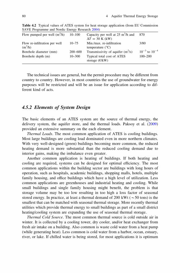
The technical issues are general, but the permit procedure may be different fromcountry to country. However, in most countries the use of groundwater for energypurposes will be restricted and will be an issue for application according to dif-ferent kind of acts.

4.5.2 Elements of System Design

The basic elements of an ATES system are the source of thermal energy, thedelivery system, the aquifer store, and the thermal loads. Paksoy et al. (2009)provided an extensive summary on the each element.

Thermal Loads. The most common application of ATES is cooling buildings.Most large buildings are cooling load dominated even in more northern climates.With very well-designed (green) buildings becoming more common, the reducedheating demand is more substantial than the reduced cooling demand due tointerior gains, making the imbalance even greater.

Another common application is heating of buildings. If both heating andcooling are required, systems can be designed for optimal efficiency. The mostcommon applications within the building sector are buildings with long hours ofoperation, such as hospitals, academic buildings, shopping malls, hotels, multiplefamily housing, and office buildings which have a high level of utilization. Lesscommon applications are greenhouses and industrial heating and cooling. Whilesmall buildings and single family housing might benefit, the problem is thatstorage volume may be too low resulting in too high a loss factor of seasonalstored energy. In practice, at least a thermal demand of 200 kWt (*50 tons) is thesmallest that can be matched with seasonal thermal storage. More recently thermalutilities which provide thermal energy to small buildings as part of a small districtheating/cooling system are expanding the use of seasonal thermal storage.

Thermal Cold Source. The most common thermal source is cold outside air inwinter. It is collected by a cooling tower, dry cooler, and/or heat exchanger fromfresh air intake on a building. Also common is waste cold water from a heat pump(while generating heat). Less common is cold water from a harbor, ocean, estuary,river, or lake. If chilled water is being stored, for most applications it is optimum

Table 4.2 Typical values of ATES system for heat storage application (from EU CommissionSAVE Programme and Nordic Energy Research 2004)

Flow pumped per well (m3/h) 10–100 Capacity per well at 25 m3/h andDT = 30 K (kW)

870

Flow re-infiltration per well(m3/h)

10–75 Min./max. re-infiltrationtemperature (�C)

3/80

Borehole diameter (mm) 200–600 Transmissivity of aquifer (m2/s) 10-3 to 10-4

Borehole depth (m) 10–300 Typical total cost of ATESstorage (€/kW)

100–200


to store as cold as possible for direct use. In practice, the minimum is *5 �C(41 �F). Any lower temperature might result in freezing water.

Thermal Heat Source. The source of heat is most commonly waste heat fromheat pumps which are being used to cool in summer months. Less common iswaste heat from cogenerators or industrial processes. Another heat source is solarthermal collected in the summer months. Direct application is not as easilyachieved since high temperatures are required by the delivery system. In thesecases, additional traditional sources are required to boast the temperature such asboilers and heat pumps.

Delivery System. The most effective and efficient HVAC system for ATES isone which separately handles latent and sensible loads during the cooling season.Fresh air intakes for most climates produce a substantial latent cooling load. Toeffectively reduce the wet bulb temperature of incoming outside air the coolantneeds to be below 12 �C. To realize the required wet bulb temperature and utilizethe stored thermal energy effectively, a larger heat exchanger than normallyapplied in the air handling unit is required with a counterflow configuration. Asecond HEX can utilize the warm water for reheating when needed. This typicallyresults in a discharge temperature of aquifer water at 18 �C.

In any event an air-to-air heat recovery system with both latent and sensibleheat recovery reduces the fresh air thermal demand and is typically included in theATES delivery system design. The sensible heat and cooling demand is oftendelivered by a radiant system or fan coil. Radiant ceilings are becoming morepopular in these cases. In this case, that the ATES system serves both for heatingand cooling, the HVAC system often includes heat pumps. In this case, the coolingload is often delivered directly with the heat pump for short peak periods when theATES system cannot provide the full load.

ATES store. The entire system including the ATES store needs to supply notonly the thermal energy for the year but also the peak thermal power. The latercriterion cannot always be cost justified. An optimum ATES system can supply thevast majority of thermal energy demand utilizing the ATES store when designed toserve as a thermal base load thermal plant.

The most important aspect of the design of wells is to ensure that surroundingproperties are not adversely affected by the ATES store. A careful configuration ofwells is required to ensure that the hydraulic head does not extend substantiallyonto adjacent properties. (e.g., change of hydraulic head not more than 30 cm atthe property boundary.) Another requirement is that the temperature change wouldnot reduce the possibility of a neighboring property owner utilizing ATES. (e.g.,temperature change not larger than 0.5 �C at the boundary.) Finally, it is criticalthat there is not a thermal breakthrough between warm (hot) and cold stores overthe long-time operation. To achieve these conditions requires a very sophisticatedand careful modeling.

The simplest system for ATES cold seasonal thermal storage utilizes a coolingtower (or dry cooler) during the winter months to charge cold wells. The coldaquifer store is then used to directly cool a building or buildings in the summer.


Such a system requires a peaking chiller to supply cold when the ATES system isnot adequate.

Optimum Systems. An example of an optimum system is one that delivers heatduring the winter at the same time generating cold water as a byproduct. Thus noextra energy is utilized to generate this chilled water.

In the winter, the water source heat pump utilizes 18 �C water stored in thesummer operating at a relative high efficiency, delivering the base load heating forthe building. In addition, when the outside temperature is below 0 �C, warm ATESwater is utilized to preheat incoming fresh air and at the same time the cold waterfrom an eventual dry cooler is stored in the ATES cold wells. When the heatingdemand cannot be fully supplied by the heat pump then a gas boiler comes on. Theamount of gas energy is typically less than 10 % of total energy demand whileabout 50 % of peak thermal demand. The dry cooler is utilized to make additionalcold water when air temperature is below 2 �C.

In the summer operation, the base load cooling is supplied directly by the ATEScold wells to both the building including the fresh air intake. When the coolingload cannot be met by the ATES cold wells the heat pump comes on. Again theATES cold wells supply the vast majority of the cooling load.

The system is designed to optimize, financially, by trading off peak load fromthe ATES system with traditional sources for short periods of time-reducing up-front investment with conventional peakers.

4.5.3 Field Investigations

One essential part in developing an ATES project is to perform site investigations.The more knowledge that is obtained of the underground properties, the betterbasis for design is achieved.

The site investigations will most commonly cover the following procedure:

• geological mapping• geophysical investigations• test drillings• pumping tests

The test drillings will define the stratigraphical units in the area while thegeophysics and geological mapping are used for extrapolation of the layers and fordefinition of geometry.

Test drillings may be a part of the final system and can be looked upon as anearly investment in system. However, more commonly they are drilled in a smalldimension and do not fit into the final system after design. In these cases, they stillcan serve as observation wells.

For shallow aquifers in the overburden it is common to drive slim steel pipesthat are perforated in the lower meter or so. This method has proven to be anexcellent way of taking samples for the design of screened production wells.


Based on the results a conceptual model is created and the hydraulic propertiesof the aquifer and its surrounding layers are derived from the pumping test. Thefinal outcome will be a geological model that is more or less accurate and that canbe used for the final design using simulation models.

To be able to make model simulations, the loads of heat and cold have to beknown. For this reason, it is common to perform measurements on how the loadsare varied at different outdoor temperatures.

Such investigations that also covers supply and return temperatures in thedistribution systems are often done prior to or in parallel with the undergroundsite investigations. The results are key factors as basis for design in order tocalculate flow rates and size of the ATES storage.

4.5.4 Model Simulations

Simulations are used for several reasons, but preferably to study how different flowrates and different number and distances between the wells are functioning. Theresults will then guide the decision where to place the wells and with what flowrate they should be operated.

The outcomes of such simulations are of two kinds, namely

• the hydraulic impact shown as cones of depression and uplift around the wells• configuration of the thermal front around the wells

4.6 History and Current Status

4.6.1 Belgium

Desmedt and Hoes (2007) and Desmedt et al. (2006) summarized the status ofATES in Belgium. ATES was introduced on the Belgian market since 1995. Since1998, many companies showed interest in the technology, but this is not translatedinto a steady increase of realized projects. This is mainly caused by the hydro-geological circumstances. In Belgium, the North-eastern part of the country hasvery good technical and economical potentials for ATES applications. However,the most interesting economical and industrial areas are located outside this region.A thick clay layer covers the Western part of Belgium; the southern part mainlyexists of Silurian schist and Devonian rock. At this time, 15 large ATES-systems([300 kW) are operational and most installations are monitored.

A number of ATES projects are monitored within the framework of asubsidy program for the stimulation of innovative energy technologies, called


‘‘Energy Demonstration Program’’. For ATES system the monitoring is three yearsin order to have representative results for steady-state performance. Enterprises canget financial support (35 % of the extra investment of the innovative investment incomparison to a traditional installation).

The implementation of the ATES technology in Belgium went unarguabletogether with some unavoidable growing pains. Some of these problems werecaused by the unusual combination of technologies and working parties. Especiallythe knowledge of hydrogeological and technical issues of ATES applications is notwell understood or not existing with engineering companies. Drilling companiesget involved in the process of HVAC installation. Most critical are the connectionpoints between the traditional and innovative installation part, defined as theboundary zone between the underground and aboveground installation. As typicalexample, the communication between the control systems of HVAC and ATESsystem can be mentioned. Other common problems are the treating of the wellsfrom time to time by the owner of the installation, the energy balance in the ground(cold storage), control problems, etc.

4.6.2 Norway

Accroding to Midttømme et al. (2008, 2009), there are about ten large AquiferThermal Energy Storage (ATES) installations. In 1987, the first known ATESsystem in Norway was established in Seljord. A 10 m-deep well was drilled forheating and cooling of Seljord lysfabrikk. The largest UTES system in Norway isat Oslo’s Gardermoen international airport. This ATES system has been in oper-ation since the airport opened in 1998 and comprises an 8 MW heat pump array,coupled to 18 wells of 45 m depth, 9 for extraction of groundwater, and 9 for re-injection. The wells are sunk into the Øvre Romerike glaciofluvial sand and gravelaquifer. This system covers the total cooling needs of the airport, of which 25 %(2.8 GWh/y) is free cooling via direct heat exchange with cold groundwater, and75 % (8.5 GWh/y) is active cooling via the use of the heat pumps. The annualheating provision is typically 11 GWh. There have been some problems withclogging of the groundwater loop, and the groundwater wells and heat exchangersrequire cleaning every few years. Because of a lack of knowledge of ATES sys-tems in Norway, Dutch consultancies were hired to design the ATES system andGSHP installations. The total cost of the system was 17 million NOK and thepayback time, compared to traditional heating and cooling systems, is estimated tobe less than 4 years.

Oslo Centre for Interdisciplinary Environmental and Social Research, a com-ponent of the Oslo Innovation Centre in Oslo, is a 13,500 m2 office building withlaboratories. An ATES system, extracting groundwater from the underlyinglimestone and shale rock, provides both heating and cooling to the building.A closed-loop BTES system was originally intended for the site, but extremelydifficult ground conditions were encountered during initial drilling: namely, zones


of remarkably high groundwater flow associated with a Permian syenite dykestructure several meters thick. It became clear that it would be both more feasibleand cheaper to drill a small number of groundwater wells (using the dyke as anaquifer) than a large number of closed-loop boreholes. Thus, a total of nine wellswere drilled. These wells are typically located in extraction-injection pairs, onewell drilled to 100 m depth and the second to 100–200 m depth. Using thisarrangement, it is possible to access enough groundwater and rock volume to coverthe seasonal cooling and heating demands of the building.

4.6.3 Sweden

The ATES systems being used in Sweden can be divided into four basic config-urations (Andersson et al. 2003). In the simplest system (A), groundwater isdirectly used for preheating of ventilation air during the winter and for coolingduring the summer season. In this case, heat and cold from ambient air is sea-sonally stored in the aquifer at a temperature level of approximately +5 �C(winter) and +15 �C (summer). More commonly used is the heat pump supportedsystem (B) that works the same way as system A. However, the production of heatis much larger and the temperature change is somewhat greater. System C rep-resents an early type of ATES applications where surface water is used as a sourceof energy for the heat pump. This heat, at a temperature of 15–20 �C, is storedduring the summer and used during the heating season. The fourth system (D) issimilar, but in this case cold from the winter is stored to be used for districtcooling.

Of these systems, heat pump supported combined heating and cooling appli-cations (system B) are dominating (65 %). However, in recent years, there is agrowing interest for storage of natural cold (system D), which is used for districtcooling applications or for industrial cooling. In Table 4.1 the recent statistics ofATES utilization are presented. It is seen that the technology is preferably used forcommercial and institutional buildings from small-scale applications to large-scaleutilization in district heating and cooling. In the industry sector only a couple ofsystems are applied for manufacturing industries. The rest represents cooling oftelecommunication installations.

The currently designed total storage capacities are in the order of 40 MW forheating and 70 MW for cooling. A rough calculation on the yearly energy turn-over, based on designed values, indicates a storage heat utilization of 120 GWhwhile the utilization of cold is about 80 GWh (Nordell et al. 2007).

Still, high temperature ATES projects are lacking in Sweden. However, recentfeasibility studies of two large-scale applications have yielded promising results.In both cases these projects are related to storage of waste heat.

A survey within Annex 13 of IEA ECES IA revealed that 40 % of the plantshave had or have operational problems or failures. The major part of these hasbeen solved by fairly simple measures. However, approximately 15 % have

4.6 History and Current Status 85

continued difficulties with well capacities. The dominating reason is clogging ofthe wells mainly caused by iron precipitation. These wells have to be treated fromtime to time. Other common problems are corrosion and malfunctioning controlsystems. In general, these types of problems are now clearly identified andunderstood, and are therefore less common in newer plants. The research inSweden has been focused on geodata collection by test drilling as one importantpart for proper well and system design. The objective with this work, which wascarried out at the Lund Institute of Technology, was to create guidelines for siteinvestigations related to ATES design. These guidelines are part of a moreextensive work with UTES guidelines that takes place within Annex 13 of IEAECES IA. These covers all aspects of design, construction, and maintenance ofUTES wells and boreholes and will be published during the autumn 2003.

From 1999, a new legislation (The New Act of Environment) was applied. ThisAct has complicated the ATES permit procedures in Sweden and it has become anobstacle for some potential ATES projects. However, the environmental benefits interms of energy conservation and economics will probably still favor a furthergrowth of ATES projects in Sweden, especially for large-scale systems.

4.6.4 Germany

Lottner and Mangold (2000), Schmidt et al. (2003, 2004), and Sanner et al. (2005)reported the status of ATES in Germany. In Germany, two aquifer heat stores arein operation in Rostock-Brinckmanshöhe and in Berlin.

In the solar assisted district heating plant of the new housing project in Rostock-Brinckmanshöhe, an aquifer is used as a low temperature seasonal store. Due to thesmall size of the plant, the shallow 30 m deep aquifer has to be operated in atemperature range between 10 and 50 �C. Model calculations for the design of theplant showed that a maximal fraction of the stored solar heat can be recovered by a100 kW heat pump. The aquifer is charged with solar heat from a 1,000 m2 solarcollector roof. A long-term monitoring program has been started in early 2000.

The district heating and cooling scheme of the renovated Reichstag buildingand of the connected neighboring large office buildings of the Parliament include ashallow and a deep aquifer, where a cold store in a depth of about 60 m and a heatstore in a depth of about 300 m. The deep aquifer is charged in summer withsurplus heat of 70 �C from the combined heat and power plants. These plants areoperated dependent on the electricity demand of the connected buildings.According to the design calculations, about 60 % of the stored heat can berecovered during the heating period from the aquifer in the temperature rangebetween 55 and 70 �C and can supplement the absorption heat pump system. Thegroundwater of the shallow aquifer is used at ambient temperature for the airconditioning of the buildings. An extensive long-term monitoring program willexamine the technical and economic feasibility of the concept.


4.6.5 The Netherlands

In the Netherlands, Aquifer Thermal Energy Storage started to be implemented inthe early 1980s (Snijders 2005). In first instance, the objective was to store solarenergy for space heating in winter. R&D activities and the first demonstrationprojects were financed within the framework of the National Research Programmeon Solar Energy (National Onderzoek Programma Zonne-energie).

In the first project, (commissioned in 1983) vertical soil heat exchangers wereused (BTES application). Given the good experience with aquifer storage in laterprojects and the fact that in the Netherlands aquifers can be found almost every-where, in particular the application of ATES has been further developed in theNetherlands. Although, ATES systems can be applied almost everywhere in theNetherlands, geographical proximity between projects and agglomeration isemerging in four provinces: North and South Holland, North Brabant and Gel-derland contain over 75 % of all projects.

In 2005, the number of registered ATES projects was 537. In almost everymajor city a number of ATES projects are in operation. The aim of most ATESprojects is to store cold in winter for cooling in summer. In general, cooling isdirect, that is to say without using a chiller. In most projects, the cooling capacitysupplied from storage lies between 500 and 2000 kWt. This means that byapplying cold storage these projects economize on a large chiller.

The heat released during cooling is stored in the aquifer also. If possible, theheat is used for heating during the winter season. This combination is called ‘‘Coldstorage and low temperature heat storage’’. The largest ATES project in operationis for supplying cooling and low temperature heat to the buildings and laboratorieson the campus of Eindhoven University. Both the cooling and heating capacity ofthe store are 20,000 kWt (5,700 tons and 68 MBtu/h respectively).

Until 2000, most ATES applications were for individual buildings like officesand hospitals. However, since about 2000 ATES also started to be applied as acentral (collective) system for a number of buildings, mixed developments, andhousing projects. At present several utility companies are offering their clients tosupply heating and cooling with ATES-based district heating and cooling systems,whereby the system is owned and managed by the utility.

Currently, the expectation is that the number of systems constructed each yearcan grow from about 100–1000 (Coenen et al. 2009). So in 2008, the Dutchgovernment formed a new actor, an ATES taskforce. This task force was asked tomake an inventory of the main barriers for implementing ATES systems. Oneproblem is the increasing geographical proximity in the underground in theNetherlands of other infrastructural systems (cables, pipes, sewers systems, tun-nels, storage systems, etc.). Another problem is the lack of a clear regulatoryframework for the use of the underground and the groundwater. Moreover, it is notclear how the government should deal with conflicting interests of different users


of the underground and groundwater. Because of this, the ATES network expressesconfusion and uncertainty about what is permitted and what not. Another barrier isthe already mentioned potential interference of systems.

4.6.6 Canada

ATES has been or is currently being implemented in a number of large-scalebuilding projects in Canada (Allen et al. 2000). Existing large installations include,for example, the Carleton University campus in Ottawa, the Sussex Hospital inNew Brunswick, and the Scarborough Centre near Toronto. Many of these havebeen operating since the late 1980s.

The Carleton University project draws its water from fractured limestoneaquifers at a temperature of about 9 �C. The project was originally designed forimplementation in four phases. Phase 1 (consisting of five wells) opened inFebruary 1990, and was constructed using standard heat-pump technology incombination with aquifer thermal energy storage. The system was designed toprovide heating and cooling for approximately 40 % of the campus buildings. Thehigh cost of energy associated by using the heat pumps prompted the university tore-assess the original design. In 1992–1993, a retrofit was undertaken in onebuilding such that it could be directly cooled during the summer months and pre-heated in the winter by a heat exchanger, without the use of heat pumps.

This new design (without heat pumps) formed the basis for an expansion to thesystem. Additional wells for Phase 2 were drilled during 1994 and were to havebeen incorporated with the existing five well system. Unfortunately, the system hasnever been implemented or tested because of non-technical administrative pro-blems. Nevertheless, two wells continue to provide heating and cooling to onebuilding.

New ATES installations are being designed for buildings operated by Envir-onment Canada in Ottawa and by Agriculture Canada in Agassiz, BritishColumbia. The Environment Canada system consists of a multiple well field, andgroundwater is extracted from a fractured sandstone aquifer at an ambient tem-perature of about 9 �C. To date, the wells have been drilled and hydraulic testingand modeling has been undertaken. Work on the building retrofit is expected totake place this year. At Agriculture Canada’s laboratory facility, five wells havebeen drilled. Four of the wells will be used for ATES, and the fifth well will act asa dump well to dispose of a small amount of excess cold water generated in thebuilding during the winter heating.

Research on ATES in Canada is limited; however, Canadian Scientists havebeen active participants in several Annexes on Energy Conservation throughEnergy Storage under the auspices of the International Energy Agency. The mostrecent Annex (13) is aimed at identifying state of the art techniques for the designconstruction and maintenance of underground thermal energy storage wells andboreholes.


There are four early ATES systems installed in Canada (Wong et al. 2006).Good amount of information has been published from these studies and this pio-neering work in ATES technology led the way in the development of ATESapplication in Canada. Through these early projects, the technical community hasidentified many challenges and also provided many learning opportunities inadvancing the technology introduction.

The earlier ATES projects included the Scarborough Canada Centre whichbegan in 1986 and studied the application of ATES for office building cooling.Later heat pumps were added to increase peak cooling and also provide someheating. Another important project was the Sussex Health Centre. This project wasfirst commissioned in 1994. It was designed for cooling with limited heating. TheCarleton University system has been in operation since 1990. The system wasdesigned for cooling and heating and operated with heat pump in the low tem-perature range. In 2002, the ATES system at the Pacific Agriculture ResearchCentre was implemented for cooling and heating using heat pump. These instal-lations helped the scientific and engineering community in getting a betterunderstanding on how the ATES systems work in the low temperature range. Themain challenges encountered were in cooling and heating load balance.

4.6.7 Denmark

As far as known, no BTES projects will be operational in Denmark by that time.The majority of the groundwater cooling projects provide direct cooling toindustrial applications. In general, the warm groundwater is reinjected into theaquifer without thermal balancing.

Recently, there is a growing interest in the application of ATES for the heatingand cooling of buildings (Hendriks et al. 2008). The first project of this kind wasoperational by the end of 2007. The major reason for this increasing interest is theintroduction of the European Energy Performance Directive for Buildings. Lack ofawareness is considered to be the major bottleneck to the application of UTEStechnologies in Denmark.

4.6.8 United Kingdom

There is only one known ATES system installed to date in the UK. The system isfor a residential development in West London and has a storage capacity of250 kW. The system was installed in 2006. By the end of 2007, there were anumber of larger scale ([500 kW) ATES and BTES systems under development,and the level of interest in UTES application is increasing. This is to a large extentattributable to recent sustainability requirements for larger scale new develop-ments and retrofits.


UTES technology is only just starting to enter into the UK market and thus isregarded as a ‘‘new’’ technology. The availability of suitable aquifers varies sig-nificantly in the UK and therefore certain areas are suitable for ATES systems andothers areas are more favorable to closed-loop BTES systems. London, the SouthEast, Birmingham, Liverpool, and East Anglia are examples of areas where ATESsystems are viable.

In the UK, the Environment Agency (EA) is the government body whichregulates the groundwater industry. Any larger scale open-loop ground sourceheating and/or cooling system has to go through the EA permitting procedure. TheEA is becoming increasingly worried about net heating or cooling effects onthe ground of GSHP’s and is therefore in favor of ground coupled systems likeATES and BTES, creating a thermal balance annually.

4.6.9 China

According to Morofsky (1994), Gao et al. (2006), applications of ATES in large-scale projects started in the 1960s, mostly in China. There were three interrelatedproblems in Shanghai that led to the development of aquifer thermal energystorage—ground subsidence, groundwater pollution, and the lack of summercooling in factories. Restrictions on groundwater extraction aimed to solve sub-sidence and pollution. However, large-scale year round injection made thegroundwater temperature unsuitable for cooling.

In 1965, cold water injection during winter started for summer cooling and hascontinued since giving 30 years of experience. Heated water is also injected forwinter heating. Experience with heat storage is also extensive with the watervolume injected being about 30 % of the cold storage volume.

By 1984, there were 492 cold storage wells in Shanghai accepting 29 millioncubic meters of water annually. Of these wells, 90 % were used for both injectionand extraction. These cold storage wells supplied textile mills, chemical works,and other industrial plants, but also commercial buildings such as the ShanghaiExhibition Hall where there are five injection wells and 1 extraction well. Most ofthese cold storage wells are 10–12 inches in diameter. The total annual coolingenergy stored in Shanghai is about 1,100 TJ. Hot water storage of waste heat ispracticed with injection temperatures as high as 400 �C. Recovery temperatures inwinter can be as high as 38 �C.

Recently Applications of ATES are fewer and fewer. The bottleneck of ATES isrecharging which is the key point of groundwater resource sustainable utilization.Low temperature ATES and heat pump technology should be combined to improveefficiency and extend development space.


4.6.10 Turkey

According to Paksoy et al. (2000, 2004) and Paksoy and Evliya (2009), R&Dactivities on the underground thermal energy storage in Turkey started with par-ticipation in IEA ECES Annex 8. UTES potential study carried out in Annex 8revealed that there is significant potential for applications in buildings (residential,commercial, and service), industry and agriculture (greenhouses) sectors. Firstfeasibility study on aquifer thermal energy storage using nearby Seyhan Lake wasrealized for the new annex of Çukurova University Hospital. 3,250 MWh ofelectricity for cooling and 1,000 tons of oil for heating were estimated to be savedannually with a calculated payback time of less than two years. In a joint study,carried out with Lulea University of Technology winter air as a cold source forborehole thermal energy storage was investigated. The ground temperature wasdecreased to 20–15 �C at the end of 3 months of cold storage in 2002–2003.

These activities were followed by a commercial ATES application in a super-market in Mersin with a heating load of 74 kW and cooling load of 195 kW. Thisproject has been in operation since 2001 with about 60 % annual energy savings.Heating and cooling potential of greenhouses in the Mediterranean climatic zone—using ATES systems was investigated in a 360 m2 greenhouse for growing toma-toes. ‘‘Zero’’ fossil fuel was consumed for the heating in winter and cooling was abonus in spring time. The yield of tomatoes was increased by 40 % with a 68 %energy savings. The calculated payback time is two years for this project.

References

AEE Institute for Sustainable Technologies (2006) High solar fraction heating and coolingsystems with combination of innovative components and methods. HIGH-COMBI

Allen DM, Ghomshei MM, Sadler-Brown TL, Dakin A, Holtz D (2000) The current status ofgeothermal exploration and development in Canada. In: Proceedings world geothermalcongress 2000, Kyushu—Tohoku, Japan, 28 May–10 June 2000

Andersson O, Hellström G, Nordell B (2003) Heating and cooling with UTES in Sweden—current situation and potential market development. FUTURESTOCK’2003, Warsaw, Poland,1–4 Sept 2003

Andersson O (2007) Aquifer thermal energy storage. In: Paksoy HÖ (ed) Thermal energy storagefor sustainable energy consumption. Springer, Dordrecht

Bauer D, Marx R, Nußbicker-Lux J, Ochs F, Heidemann W, Müller-Steinhagen H (2010) Germancentral solar heating plants with seasonal heat storage. Sol Energy 84(4):612–623

Bridger DW, Allen DM (2005) Designing aquifer thermal energy storage systems. ASHRAE J47(9):S32–S37

Buik N, Snijders AL (2006) Clogging rate of recharge wells in porous media. In: Proceedingsmegastock, Pomona, NJ, U.S.A., 13 May–2 June 2006

Coenen L, Raven R, Verbong G (2009) Local niche experimentation in energy transitions: atheoretical and empirical exploration of proximity advantages and disadvantages. Centre forInnovation, Research and Competence in the Learning Economy (CIRCLE), Lund University,Lund, Sweden


Desmedt J, Hoes H (2007) Monitoring results of aquifer thermal energy storage system in aBelgian hospital. In: AIVC 28th conference and Palenc 2nd conference: building low energycooling and ventilation technologies in the 21st century, Crete island, Greece, 27–29 Sept 2007

Desmedt J, Hoes H, Van Bael J (2006) Status of underground thermal energy storage in Belgium.Ecostock 2006, Pomona, NJ, USA, 31 May–2 June 2006

Dickinson JS, Buik N, Matthews MC, Sntjders A (2009) Aquifer thermal energy storage:theoretical and operational analysis. Geotechnique 59(3):249–260


Gao Q, Li M, Jiang Y, Li M, Yu M, Qiao G (2006) Practice and task developing undergroundthermal energy storage in China. Ecostock 2006, Pomona, NJ, USA, 31 May–2 June 2006

Hendriks M, Snijders A, Boid N (2008) Underground thermal energy storage for efficient heatingand cooling of buildings. In: Proceedings of the 1st international conference on industrialised,integrated, intelligent construction (I3CON), Loughborough, UK, 14–16 May 2008

Jenne EA, Andersson O, Willemsen A (1992) Well, hydrology, and geochemistry problemsencountered in ATES systems and their solutions. Report Prepared for the U.S. Department ofEnergy

Lottner V, Mangold D (2000) Status of seasonal thermal energy storage in Germany.TERRASTOCK 2000, Stuttgart, Germany, 28 Aug–1 Sept 2000

Midttømme K, Banks D, Ramstad RK, Sæther OM, Skarphagen H (2008) Ground-source heatpumps and underground thermal energy storage-energy for the future. In: Slagstad T (ed)Geology for society, geological survey of Norway special publication, vol 11. Norway,pp 93–98

Midttømme K, Hauge A, Grini RS, Stene J, Skarphagen H (2009) Underground thermal energystorage (UTES) with heat pump in Norway. Proceedings of Effstock 2009. Stockholm,Sweden, 15–17 June 2009

Morofsky EL (1994) ATES-energy efficiency, economics, and the environment. In: Proceedingsof international symposium on aquifer thermal energy storage, Tuscaloosa, AL, USA, 14–15Nov 1994

Nordell B, Grein M, Kharseh M (2007) Large-scale utilisation of renewable energy requiresenergy storage. In: International conference for renewable energies and sustainabledevelopment (ICRESD_07), Université Abou Bakr BELKAID—TLEMCEN; Algeria,21–24 May 2007

Nielsen K (2003) Thermal energy storage. A state-of-the-art. NTNU, TrondheimPaksoy HÖ, Andersson O, Abaci S, Evliya H, Turgut B (2000) Heating and cooling of a hospital

using solar energy coupled with seasonal thermal energy storage in aquifer. Renew Energy19(1–2):117–122

Paksoy HÖ, Gürbüz Z, Turgut B, Dikici D, Evliya H (2004) Aquifer thermal storage (ATES) forair-conditioning of a supermarket in Turkey. Renew Energy 29(12):1991–1996

Paksoy HÖ, Evliya H (2009) Thermal energy storage activities in Turkey. Proceedings ofEffstock 2009, Stockholm, Sweden, 15–17 June 2009

Paksoy HÖ, Snijders A, Stiles L (2009) State-of-the-art review of aquifer thermal energy storagesystems for heating and cooling buildings. In: Proceedings of Effstock 2009, Stockholm,Sweden, 15–17 June 2009

Phetteplace G (2007) Geothermal heat pumps. J. Energy Eng 133(1):32–38Sanner B, Kabus F, Seibt P, Bartels J (2005) Underground thermal energy storage for the German

parliament in Berlin, system concept and operational experiences. In: Proceedings worldgeothermal congress 2005. Antalya, Turkey, 24–29 April 2005

Schmidt T, Mangold D, Müller-Steinhagen H (2003) Seasonal thermal energy storage inGermany. ISES Solar World Congress 2003, Göteborg, Sweden, 14–19 June 2003

Schmidt T, Mangold D, Müller-Steinhagen H (2004) Central solar heating plants with seasonalstorage in Germany. Sol Energy 76(1–3):165–174


Snijders AL (2005) Aquifer thermal energy storage in the Netherlands status beginning of 2005.IFTech International B.V, Arnhem

Wong B, Snijders A, McClung L (2006) Recent inter-seasonal underground thermal energystorage applications in Canada. EIC climate change technology, 2006 IEEE, Ottawa, ON,Canada, 10–12 May 2006

References 93

Chapter 5Borehole Thermal Energy Storage

5.1 Definition

If it is impossible to exploit a suitable aquifer for energy storage, a borehole thermalenergy storage system (BTES) can be considered. Vertical ground heat exchangers(GHE), also called borehole heat exchangers (BHE) are widely used when there is aneed to install sufficient heat exchange capacity under a confined surface area suchas where the Earth is rocky close to the surface, or minimum disruption of thelandscape is desired. This is possible because the temperature below a certain depthremains relatively constant over the year. In a standard borehole, which in typicalapplications is 20–300 m deep, plastic pipes made of polyethylene or polypro-pylene are installed. The space between the pipe and the hole is filled with anappropriate material to ensure good contact between the pipe and the undisturbedground and reduce the thermal resistance (Florides and Kalogirou 2007). Figure 5.1shows a side view of borehole thermal energy storage tube.

Vertical loops are generally more expensive to install, but require less pipingthan horizontal loops because the Earth deeper down is cooler in summer andwarmer in winter, compared to the ambient air temperature.

With borehole storage, vertical borehole heat exchangers are inserted into theunderground, which ensure the transfer of thermal energy toward and from theground (clay, sand, rock, etc.). Many projects are about the storage of solar heat insummer for space heating of houses or offices. Ground heat exchangers are alsofrequently used in combination with heat pumps (‘‘geothermal heat pump’’), wherethe ground heat exchanger extracts low-temperature heat from the soil (Interna-tional Energy Agency 2006).

BTES makes use of long boreholes that are dug into the ground. Thermalenergy is transferred to the underground by means of conductive flow from anumber of closely spaced boreholes. The boreholes can be equipped with differentkinds of borehole heat exchangers, making the boreholes act as a large heatexchanger between the system and the ground. Each borehole contains a U-tubewhich links together with a central piping system at the surface. Sometimes more


95

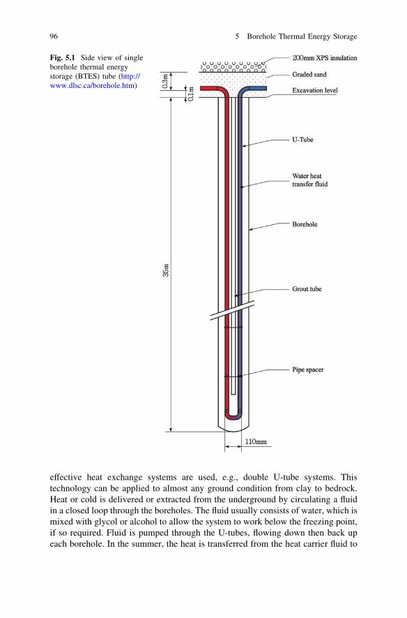
effective heat exchange systems are used, e.g., double U-tube systems. Thistechnology can be applied to almost any ground condition from clay to bedrock.Heat or cold is delivered or extracted from the underground by circulating a fluidin a closed loop through the boreholes. The fluid usually consists of water, which ismixed with glycol or alcohol to allow the system to work below the freezing point,if so required. Fluid is pumped through the U-tubes, flowing down then back upeach borehole. In the summer, the heat is transferred from the heat carrier fluid to

Fig. 5.1 Side view of singleborehole thermal energystorage (BTES) tube (http://www.dlsc.ca/borehole.htm)

96 5 Borehole Thermal Energy Storage

http://www.dlsc.ca/borehole.htm


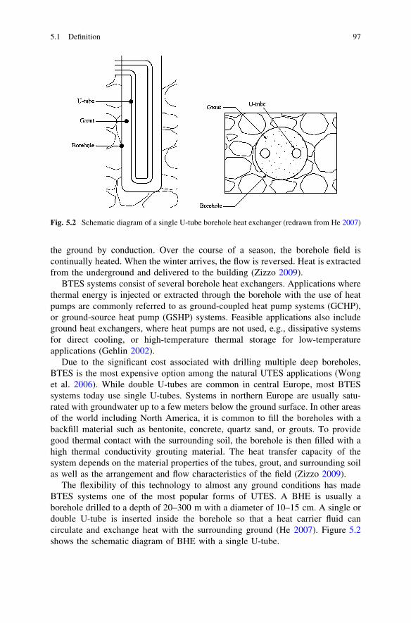
the ground by conduction. Over the course of a season, the borehole field iscontinually heated. When the winter arrives, the flow is reversed. Heat is extractedfrom the underground and delivered to the building (Zizzo 2009).

BTES systems consist of several borehole heat exchangers. Applications wherethermal energy is injected or extracted through the borehole with the use of heatpumps are commonly referred to as ground-coupled heat pump systems (GCHP),or ground-source heat pump (GSHP) systems. Feasible applications also includeground heat exchangers, where heat pumps are not used, e.g., dissipative systemsfor direct cooling, or high-temperature thermal storage for low-temperatureapplications (Gehlin 2002).

Due to the significant cost associated with drilling multiple deep boreholes,BTES is the most expensive option among the natural UTES applications (Wonget al. 2006). While double U-tubes are common in central Europe, most BTESsystems today use single U-tubes. Systems in northern Europe are usually satu-rated with groundwater up to a few meters below the ground surface. In other areasof the world including North America, it is common to fill the boreholes with abackfill material such as bentonite, concrete, quartz sand, or grouts. To providegood thermal contact with the surrounding soil, the borehole is then filled with ahigh thermal conductivity grouting material. The heat transfer capacity of thesystem depends on the material properties of the tubes, grout, and surrounding soilas well as the arrangement and flow characteristics of the field (Zizzo 2009).

The flexibility of this technology to almost any ground conditions has madeBTES systems one of the most popular forms of UTES. A BHE is usually aborehole drilled to a depth of 20–300 m with a diameter of 10–15 cm. A single ordouble U-tube is inserted inside the borehole so that a heat carrier fluid cancirculate and exchange heat with the surrounding ground (He 2007). Figure 5.2shows the schematic diagram of BHE with a single U-tube.

Fig. 5.2 Schematic diagram of a single U-tube borehole heat exchanger (redrawn from He 2007)

5.1 Definition 97

A BTES system consists of an array of boreholes resembling standard drilledwells. The holes can be drilled either in a quadratic or a hexagonal pattern, andthey are usually vertical. A hexagonal pattern is better with regard to energytransmission and heat losses in the rock mass, but a square pattern is simpler todrill and connection between boreholes is easier. The distance between theboreholes will among other factors depend on the thermal properties of the rock.Distances of 6–8 m are quite common in Scandinavian rock types (Nielsen 2003)

The holes can be connected in serial configuration, in parallel, or in a combi-nation serial/parallel depending on the planned thermal loading and unloading ofthe facility. The shape of the storage facility, seen at the surface, can be adapted tothe shape of the available land area as illustrated in Fig. 5.3.

From a depth of some 10 m, the underground has an ambient temperature that ispractically constant throughout the year and normally related to the mean annualair temperature. At further depths, the temperature will increase with the geo-thermal gradient, normally with 1–3 �C per 100 m. In some BTES applications,the ambient ground temperature can be directly used for free natural coolingpurposes. Such systems are regarded as passive in the sense that they are naturallyrecharged. However, in most cases cold has to be actively stored in the soil androck mass to provide the temperature that is demanded. These actively rechargedsystems are regarded as true BTES applications.

In the true BTES systems, natural or artificial cold is stored during the winter byextracting heat from the underground, practically always by operating a heatpump. During the summer, the chilled rock will deliver free cooling and slowly beheated up again. In some cases, the heat pump is used as a chiller to cover peakload demands. Figure 5.4 explains BTES operations for cooling and heating(http://underground-energy.com/BTES.html).

In the cold season, the heat stored in the outside of the array is used for heating.Water from the store at around 15–20 �C is passed through a heat pump, which inturn provides water around 40–50 �C for use in building heating.

Fig. 5.3 Examples of different drilling patterns that may be used in a BTES facility (redrawnfrom Nielsen 2003)


http://underground-energy.com/BTES.html

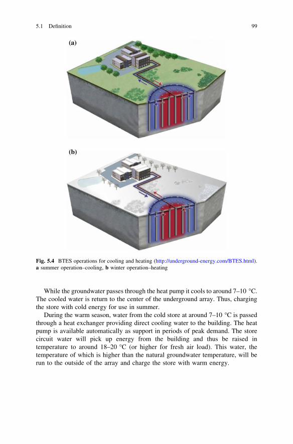
While the groundwater passes through the heat pump it cools to around 7–10 �C.The cooled water is return to the center of the underground array. Thus, chargingthe store with cold energy for use in summer.

During the warm season, water from the cold store at around 7–10 �C is passedthrough a heat exchanger providing direct cooling water to the building. The heatpump is available automatically as support in periods of peak demand. The storecircuit water will pick up energy from the building and thus be raised intemperature to around 18–20 �C (or higher for fresh air load). This water, thetemperature of which is higher than the natural groundwater temperature, will berun to the outside of the array and charge the store with warm energy.

Fig. 5.4 BTES operations for cooling and heating (http://underground-energy.com/BTES.html).a summer operation–cooling, b winter operation–heating

5.1 Definition 99


The performance factor of heat pump supported BTES systems will normallybe in the range 4–5, depending on the amount of cold produced in the system. Thecold production (free cooling) in itself is normally around 20–30. The paybacktime for these kinds of systems ranges between 5 and 10 years, depending on sizeand other circumstances (EU Commission SAVE Programme and Nordic EnergyResearch 2004). This is significantly higher than that for ATES, but on the otherhand, the operational risks are much lower.

In recent years, a third kind of system, known as ‘‘the American’’, has beenintroduced in Europe. In this system, both the condenser (cooling mode) and theevaporator (heating mode) of the heat pump are connected to the boreholes.Hence, the heat pump serves as both a heater and a chiller. During cold production,the waste heat is stored in the underground, and during heat production waste coldis stored. These systems are preferably designed for the cooling load, and theadvantage is that they do not need any peak load coverage. The heat rejection fromthe condenser during cooling can be performed at higher temperatures (25–32 �C)in the ground loop than during free natural cooling (10–15 �C). This requires lessborehole length per installed cooling capacity than free cooling systems, but at thesame time, the heat pump is larger (for the same application), and the performancefactor is somewhat lower (since the cooling is performed with the heat pump).

The BHE is the most common practice used for GHE installations because itrequires a relatively small land area for installation. Moreover, the ground tem-perature and thermal properties are more constant in the deep ground, thusresulting in a higher heat transfer rate for the BHE. The heat transfer process of theBHE is very complicated, and the heat transfer rate of the BHE depends on anumber of factors including the ground thermal properties, moisture content,regional groundwater flow, the installation and the arrangement of the heatexchanger including the grout material, the U-tube configuration, and the spacingand the depth of the boreholes. In order to properly and accurately design orevaluate the systems, modeling the BHE is the first and the most important step.By making various simplifications and assumptions, different methods have beendeveloped to model the BHE.

BTES can achieve coefficient of performance (COP) values from 4 to about 8,compared to COP values of around 3.5 for a conventional GSHP geothermalinstallation (http://underground-energy.com/BTES.html). The capital cost of alarge BTES system can be significant, as a large number of geothermal boreholeswill need to be drilled compared to just a few thermal wells for an ATES system.However, the installation cost should be similar to conventional GSHP systems,and the higher COP values will result in a lower total life cycle-cost than aconventional GSHP system. Both closed-loop geothermal systems will have alower life-cycle cost than a conventional fossil-fuel fired HVAC system. BecauseBTES is a closed-loop geothermal technology, there should be little difficulty inobtaining permits. Typically, the most common constraint is on the available landarea in which to construct the GHX array.



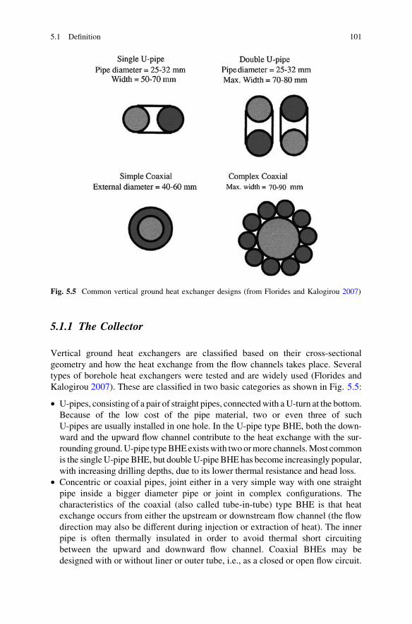
Fig. 5.5 Common vertical ground heat exchanger designs (from Florides and Kalogirou 2007)

5.1.1 The Collector

Vertical ground heat exchangers are classified based on their cross-sectionalgeometry and how the heat exchange from the flow channels takes place. Severaltypes of borehole heat exchangers were tested and are widely used (Florides andKalogirou 2007). These are classified in two basic categories as shown in Fig. 5.5:

• U-pipes, consisting of a pair of straight pipes, connected with a U-turn at the bottom.Because of the low cost of the pipe material, two or even three of suchU-pipes are usually installed in one hole. In the U-pipe type BHE, both the down-ward and the upward flow channel contribute to the heat exchange with the sur-rounding ground. U-pipe type BHE exists with two or more channels. Most commonis the single U-pipe BHE, but double U-pipe BHE has become increasingly popular,with increasing drilling depths, due to its lower thermal resistance and head loss.

• Concentric or coaxial pipes, joint either in a very simple way with one straightpipe inside a bigger diameter pipe or joint in complex configurations. Thecharacteristics of the coaxial (also called tube-in-tube) type BHE is that heatexchange occurs from either the upstream or downstream flow channel (the flowdirection may also be different during injection or extraction of heat). The innerpipe is often thermally insulated in order to avoid thermal short circuitingbetween the upward and downward flow channel. Coaxial BHEs may bedesigned with or without liner or outer tube, i.e., as a closed or open flow circuit.

5.1 Definition 101

5.1.2 Borehole Filling

A vertical borehole may require that some kind of backfilling material is used tofill the space between the flow channels and the borehole wall. The filling materialprovides a good thermal contact with the surrounding ground due to low thermalconductivity of natural filling material or low groundwater level. Anotherimportant issue is to limit vertical water movement along the borehole to avoidmigration of polluted water, drainage of soil layers near the ground surface, anddisturbance of the hydraulic characteristics of artesian formations. There is noregulation.

Special grouts are used to provide a low permeability. It is important that thesegrouts have the capability to bond against both borehole wall and pipes. Themixtures must be workable and pumpable during installation with little shrinkageduring settling. If shrinkage occurs, this may cause a pathway for fluid migration.Common grouts, such as bentonite, usually have low thermal conductivity. Specialgrouts have been developed to enhance the thermal conductivity.

Laboratory tests to investigate thermal resistance and thermal conductivity ofgrouts have been reported by various authors and the results provide a goodoverview of experience on grouted boreholes and various grouts (Florides andKalogirou 2007).

In Sweden and Norway, it is most common to leave the boreholes ungrouted,i.e., the boreholes are filled with groundwater. Boreholes are commonly drilled inhard rock with the groundwater table a few meters below ground surface. Stagnantwater has low thermal conductivity, however thermal gradients that will neces-sarily occur in BHEs cause natural convection, thus enhancing the heat transferbetween the heat exchanger and the surrounding ground.

5.2 Applications

Borehole systems (BTES) are the most generally applicable UTES. In such sys-tems, bedrock is used as the storage medium. The boreholes that penetrate thestorage volume are heat exchangers of the system, through which a heat carrier ispumped. A pipe system is installed in the borehole to enable the circulation of aheat carrier. When thermal energy is injected the temperature of the storagemedium is increased.

Nordell (2000) summarized the various applications of the BTES system.

• Small-scale systems:

– Single borehole for cooling (with and without recharge)– Single borehole for heating with heat pump (with and without recharge)– Single borehole for heating with heat pump and direct cooling


• Large-scale systems:

– System of Boreholes for heat extraction with heat pump– System of Boreholes for heat extraction with heat pump and recharge of

extracted energy

• Borehole Storage Systems

– Seasonal loading of thermal energy (heat or cold) for later extraction– Seasonal loading of thermal energy for the purpose of cooling or heating of

the ground

BTES systems are most suitable for base load operation, both when loading andunloading the store. It is mainly for seasonal storage. The theory of BTES wassummarized by Hellström (1991).

Many hundreds of thousands of BTES systems have been constructed aroundthe world. The Geothermal Heat Pump Consortium (GHPC) estimates that 400,000BTES systems would annually be built in US within a few years. Most of them areborehole systems of one or a few boreholes. There are however an increasingnumber of large-scale systems i.e., more than 10–20 boreholes.

5.3 Market Opportunities and Barriers

The problems often encountered with BHE design include inadequate address offlow, pressure drop, and control parameters, leaks associated with corrosion offittings, poor workmanship, as well as the selection of pipe materials and of thecirculated heat transfer fluid (Sanner et al. 2003). All of the above require theexpertise of an engineer and contractor qualified in the installation of ground-sourceheat pumps, which represents a significant barrier to their market penetration. Incountries with higher sales of geothermal heat pumps such as Sweden, Switzerland,and Germany, technical guidelines, contractor certifications, and quality awards,etc., are beginning to be set into force to protect the industry and the consumersagainst poor quality and insufficient longevity of geothermal heat pump systems.

5.4 Analysis of Ground Thermal Behavior

Heat flow, which is a measure of the amount of thermal energy coming out of theEarth, is calculated by multiplying the geothermal gradient by the thermal con-ductivity of the ground. Each rock type has a different thermal conductivity, whichis a measure of the ability of a material to conduct heat. Quartz-rich rock likesandstone, has a high thermal conductivity, which indicates that heat readily passesthrough them. Rocks that are rich in clay or organic material, like shale and coal,have low thermal conductivity, meaning that heat passes slower through these

5.2 Applications 103

layers. If the heat flow is constant throughout a drill hole (i.e., water is not flowingup or down the hole), then it is obvious that low-conductivity shale layers willhave a higher geothermal gradient compared to high-conductivity sandstone layers(Florides and Kalogirou 2007).

Proper design of borehole heat exchangers (BHE) for commercial and institu-tional buildings utilizing ground-source heat pump systems requires a good esti-mate of the thermal conductivity of the ground in order to avoid significantlyoversizing or undersizing the ground heat exchanger (Gehlin and Spitler 2003).A good estimate of the thermal conductivity is also needed when designing aBTES system. The ground thermal properties may be measured in situ at a specificlocation using thermal response test.

In a thermal response test, a constant heat injection or extraction is imposed ona test borehole. The resulting temperature response can be used to determine theground thermal conductivity, and to test the performance of boreholes. The firstmobile measurement devices for thermal response testing were independentlyconstructed in Sweden and the USA, in 1995.

Different mathematical models—analytical and numerical—are used for theevaluation of response test temperature data (Yang et al. 2010). The differentmodels require somewhat different sets of input data.

5.4.1 Heat conduction Outside Borehole

A number of simulation models for the heat transfer outside the borehole have beenrecently reported, most of which were based on either analytical methodologies ornumerical methods. A few models were developed based on the incorporation ofthe analytical and numerical solutions.

He (2007) and Yang et al. (2010) classified and summarized basic approachesused to simulate BHEs. One is the analytical method, like the line-source model(Ingersoll et al. 1954) and the cylindrical model (Carslaw and Jaeger 1959),another one being the response factor method such as Eskilson’s model (Eskilson1987), Helltröm’s model (Hellström 1991) and Yavuzturk’s model (Yavuzturk1999), The third one is the numerical method, for example Gu’s model (Gu andO’Neal 1998) and Zeng’s model (Zeng et al. 2003).

5.4.1.1 Line-Source Model

The earliest approach to calculate the thermal transport around a heat exchangepipe in the ground is the Kelvin line-source theory assuming the infinite linesource. In the Kelvin’s line-source theory, the ground is regarded as an infinitemedium with an initial uniform temperature.

The borehole is assumed as an infinite line source. The heat transfer in thedirection of the borehole axis, including the heat flux across the ground surface and


down the bottom of the borehole, is neglected. The heat conduction process in theground can be, therefore, simplified as one-dimensional one.

Ingersoll et al. (1954) developed the line-source model, assuming the boreholeas a line source which is infinitely long and the heat flow is all normal to the linesource with a constant flux. This is the basic model used to calculate the heattransfer between the line source and the ground, and a lot of other modelsdeveloped by further researchers are basically based on the line-source model. Ifthe line source starts at zero time and the medium is at an initially uniformtemperature, the expression given by Ingersoll for the temperature at any time t atany point can be written as:

T � To ¼Q0

2pk

Z 1

X

e�b2

bdb � Q0

2pkI Xð Þ ð5:1Þ

where b ¼ r2ffiffiffiffiffiffiffiffiffiffia t�t0ð Þp X ¼ r

2ffiffiffiatp

By applying this line-source model, Ingersoll et al. (1954) studied the system ofground heat exchangers with heat pumps, and it was reported that in general, theagreement of the theory and experiment was acceptable.

Although it is characterized by the simplicity and less computation time, thismodel can only be applied to small pipes within a narrow range of a few hours tomonths because of the assumption of the infinite line source. It was estimated thatthe application of Kelvin’s line source may cause a noticeable error when asatr2

b\20.

This approach has been widely utilized in some analytical design methods thatare currently used to analyze the heat transfer of GHEs. A number of improve-ments for this approach have been proposed to account for some complicatedfactors so that the accuracy can be comparable to that of the numerical methods.

However, in the line-source model, the borehole was treated as an infinite linesource. The borehole geometry, thermal properties, and the mass and otherproperties of the fluid had not been accounted for. The outlet temperature of thefluid can only be obtained with the same approximation that is used by Eskilson(1987) and Yavuzturk (1999). Moreover, since the line-source model is a one-dimensional model, it does not directly provide a method for predicting theinterference between the boreholes. The assumption that the borehole is infinitelylong ignores the end effects, which will cause some error in the long term. Lastly,the line-source model has low accuracy at short (e.g. hourly) time steps.

5.4.1.2 Cylinder Source Model

Based on the Eskilson (1987)’s model, an analytical solution to the finite linesource has been developed by considering the influences of the finite length ofthe borehole and the ground surface as a boundary. The following assumptions aretaken in the analytical model in order to derive an analytical solution.

5.4 Analysis of Ground Thermal Behavior 105

• The ground is regarded as a homogeneous semi-infinite medium with constantthermophysical properties.

• The boundary of the medium, i.e., the ground surface, keeps a constant tem-perature (To), same as its initial one throughout the time period concerned.

• The radial dimension of the borehole is neglected so that it may be approxi-mated as a line-source stretching from the boundary to a certain depth, H.

• As a basic case of study, the heating rate per length of the source, ql, is constantsince the starting instant, t ¼ 0

Carslaw and Jaeger (1959) solved the problem on the infinite circular cylinder bythe Laplace transformation method. Assuming a constant flux Q0 along the boreholero and the borehole is infinite long, the governing equation for one-dimensional heattransfer problem in the cylindrical coordinate can be expressed as:

o2hor2þ 1

r

ohor� 1

aohot¼ 0 ro\r\1 ð5:2Þ

while the boundary conditions and initial condition can be expressed as:

�2prokohor¼ Q0 r ¼ ro; t [ 0 ð5:3Þ

ohor¼ 0 r ¼ 0 ð5:4Þ

h ¼ 0 r [ ro; t ¼ 0 ð5:5Þ

where h ¼ T � To

Taking the Laplace transform and the inverse Laplace transform, the solution is

h r; tð Þ ¼ 2Q0

pk

Z1� e�au2t� � J0 u; rð ÞY1 uað Þ � Y0 urð ÞJ1 uað Þ

u2 J21 uað Þ þ Y2

1 uað Þ� � du ð5:6Þ

where J0; J1; Y0; Y1 are the zero and the first order of Bessel functions, respectively.The solution of the temperature excess was given by Zeng et al. (2003):

h ¼ ql

4kp

Z H

0

erfc

ffiffiffiffiffiffiffiffiffiffiffiffiffiffiffiffir2þ z�hð Þ2p

2ffiffiffiffiasp

� �

ffiffiffiffiffiffiffiffiffiffiffiffiffiffiffiffiffiffiffiffiffiffiffiffiffiffir2 þ z� hð Þ2

q �erfc

ffiffiffiffiffiffiffiffiffiffiffiffiffiffiffiffir2þ zþhð Þ2p

2ffiffiffiffiasp

� �

ffiffiffiffiffiffiffiffiffiffiffiffiffiffiffiffiffiffiffiffiffiffiffiffiffiffir2 þ zþ hð Þ2

q

8>><

>>:

9>>=

>>;dh ð5:7Þ

It can be seen from Eq. 5.7 that the temperature on the borehole wall, wherer ¼ ro, varies with time and borehole depth. The temperature at the middle of theborehole depth (z ¼ 0:5H) is usually chosen as its representative temperature. Analternative is the integral mean temperature along the borehole depth, which maybe determined by numerical integration of Eq. 5.7. For the convenience ofapplications, the former is usually accepted as the representative temperature in thedesign and analysis program. It is obvious that the integral of Eq. 5.7 can be


computed much faster than the numerical solution of the same heat conductionproblem in the semi-infinite domain with long duration. The methodology hasbeen complied in the later design and simulation software developed by otherresearchers.

Comparing the cylinder source model with the line-source model, it can beobserved that during the unsteady-state heat transfer process, the results by theline-source model were delayed. It was because the line-source model assumedthe heat flux was on the central line of the borehole (r ¼ 0), while the cylindersource model assumed the heat flux was on the borehole surface (r ¼ ro), whichwas closer to the actual heat transfer process.

However, similar to the case of the line-source model, the cylinder sourcemodel ignored the heat transfer inside the borehole, for example the heat transferbetween the fluid and the U-tube, the U-tube and the grout, and the grout and theborehole. Thus, only with the same assumption used by Eskilson (1987) andYavuzturk (1999), the model can be used to obtain the fluid temperature, which isthe critical factor in the evaluation of system performance. Moreover, due to theassumption of the infinite length of the cylinder, it has the same limitations as theline-source model.

5.4.1.3 Eskilson’s Model

Eskilson’s model was developed to analyze the ground heat exchanger response,i.e., the relation between heat extraction rate and temperature of the fluid circu-lating inside the U-tube (Eskilson 1987). It was totally neglected in both the line-source model and the cylinder source model. First, the thermal process of a singleborehole was analyzed using an analytical method. Then the thermal interactionbetween boreholes was investigated, and the thermal resistance was modified bydimensionless time response factors, called g-functions. A numerical model forany configuration of boreholes was developed, and the superposition method wasused to solve for the thermal influence of multiple boreholes, while the heattransfer process along the borehole was determined by an analytical solution.Several assumptions and simplifications were used in Eskilson’s model; (1) Theannual mean air temperature To was considered to be the ground surface tem-perature. (2) The ground was assumed to be homogeneous. (3) The uppermost partof the borehole was treated as thermally insulated. (4) The borehole temperature Tb

was assumed to be constant along the borehole depth.Accounting for the assumptions above, the thermal process of a single borehole

can be expressed by the heat conduction equation, and the mathematical equationin cylindrical coordinates can be expressed as:

1a

oT

ot¼ o2T

or2þ 1

r

oT

orþ o2T

oz2ð5:8Þ


The boundary conditions at the ground surface and the initial condition weregiven as follows:

T r; 0; tð Þ ¼ To

T r; z; 0ð Þ ¼ To

T r;1; tð Þ ¼ To

oT

or0; z; tð Þ ¼ 0

And the boundary condition of the borehole temperature was assumed to beconstant over the borehole length H:

T rb; z; tð Þ ¼ Tb tð Þ D\z\Dþ H ð5:9Þ

By considering the heat extraction or dissipation as a step function Q tð Þ, thetemperature response of any heat input can be calculated using a basic step pulse,and the solution can be obtained by superimposing the responses in time as a seriesof step pulses. Figure 5.6 shows the schematic diagram of the step function and thestep pluses. Converting the temperature responds to a series of dimensionlesstemperature response factors, called g-functions, it was possible to calculate thetemperature change at the borehole in response to a single heat step pulse.Superimposing the responds of any heat extraction or dissipation, the boreholetemperature can be determined.

Tb tð Þ ¼ To þXn

i¼1

Qi � Qi�1

2pkg

tn � ti�1

ts;rb

H

ð5:10Þ

The finite line-source model was used to approximate the g-functions for dif-ferent borehole configurations, and each finite source solution was calculatednumerically with finite difference method. The basic time-scale for the borehole

process was introduced as5r2

ba and the heat transfer rate below this time-scale was

considered with a very low accuracy. The typical time-scale used in Swedishapplications was of the order of 2 h (Eskilson 1987), while Yavuzturk (1999)

Fig. 5.6 Schematic diagramof heat step functions andstep pulses (from He 2007)


reported it was 3–6 h for a typical borehole. Eskilson (1987) had reported thedifferent g-functions for 226 cases in his studies, and the guidelines for optimizingthe configuration were given.

5.4.1.4 Hellström’s model

Hellström (1991) developed the duct storage (DST) model to investigate thethermal response of the ground heat exchanger, i.e., the relation between the heattransfer rate and the temperature of the fluid circulating inside the U-tube. Therewere two basic assumptions for the thermal analyses; (1) Only heat conductiontook place in the ground. (2) The ground was homogenous or the subregion of theground was homogenous. Hellström divided the heat transfer process into threesubprocesses: (1) the thermal process between heat carrier fluid and the groundimmediately outside the heat exchanger, (2) the heat exchanger interacting withthe surrounding ground in a local thermal process, and (3) the global processinvolving the storage volume and the surrounding ground. A single fluid-to-groundthermal resistance was employed to calculate the heat transfer from the fluid to theground. The temperature difference between the fluid and the ground was deter-mined by an analytical solution, while the local and the global process were solvedby using the finite difference method. In the local process, the heat injection ratewas approximated by a step-wise constant value, and by superposition, it wasregarded as a series of simple heat injection steps. Due to symmetry, the heat fluxthrough boundaries of the local region around a ground heat exchanger wasconsidered to be zero, and the temperature in this region increased linearly withtime. The global process dealt with three fundamental components: a transient heatloss through the storage boundaries during the initial years, a steady-state value ofheat loss being gradually approached, and also a superimposed periodic variationduring the storage cycle. For computational accuracy and efficiency, the DSTmodel was implemented as a component of TRNSYS, a well-known transientsystem simulation program.

5.4.1.5 Gu’s Model

In order to incorporate the thermal interference between the two pipe legs of theU-tube into the analytical solution of the cylindrical source model, Gu and O’Neal(1998) developed an expression for the equivalent diameter of a vertical U-tubeheat exchanger. For a steady-state operation, the two legs of a U-tube were con-sidered as two constant cylindrical heat sources. One of the legs was assumed to beconcentric with the grout and the thermal influence from the other leg was esti-mated using the principle of superposition, since the heat conduction equationswere linear. Based on the concept of equivalent external thermal resistance (ETR),an expression for the equivalent diameter can be achieved. Figure 5.7 shows thediagram of the equivalent diameter of a single U-tube.


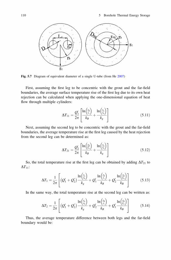
First, assuming the first leg to be concentric with the grout and the far-fieldboundaries, the average surface temperature rise of the first leg due to its own heatrejection can be calculated when applying the one-dimensional equation of heatflow through multiple cylinders:

DT11 ¼Q012p

ln rbrc

� �

kBþ

ln rcrb

� �

kg

2

4

3

5 ð5:11Þ

Next, assuming the second leg to be concentric with the grout and the far-fieldboundaries, the average temperature rise at the first leg caused by the heat rejectionfrom the second leg can be determined as:

DT21 ¼Q022p

ln rbLs

� �

kBþ

ln rcrb

� �

kg

2

4

3

5 ð5:12Þ

So, the total temperature rise at the first leg can be obtained by adding DT21 toDT11:

DT1 ¼1

2pQ01 þ Q02� � ln rc

rb

� �

kgþ Q01

ln rbrc

� �

kBþ Q02

ln rbLs

� �

kB

2

4

3

5 ð5:13Þ

In the same way, the total temperature rise at the second leg can be written as:

DT2 ¼1

2pQ01 þ Q02� � ln rc

rb

� �

kgþ Q02

ln rbrc

� �

kBþ Q01

ln rbLs

� �

kB

2

4

3

5 ð5:14Þ

Thus, the average temperature difference between both legs and the far-fieldboundary would be:

Fig. 5.7 Diagram of equivalent diameter of a single U-tube (from He 2007)


D�T ¼ DT1 þ DT2

2¼ Q01 þ Q02

2p

ln rbffiffiffiffiffiffiraLsp� �

kBþ

ln rcrb

� �

kB

2

4

3

5 ð5:15Þ

The ETR value of the U-tube can then be obtained by dividing Eq. 5.15 by thetotal heat transfer rate, Q01 þ Q02:

ETRð Þtotal¼1

2p

ln rbffiffiffiffiffiffiraLsp� �

kBþ

ln rcrb

� �

kB

2

4

3

5 ð5:16Þ

For a pipe with the equivalent diameter, the ETR can be written as:

ETRð Þeq¼1

2p

ln rbffiffiffiffireqp� �

kBþ

ln rcrb

� �

kB

2

4

3

5 ð5:17Þ

By comparing Eqs. 5.16 and 5.17, the following expression for the equivalentdiameter can be obtained:

Deq ¼ 2req ¼ 2ffiffiffiffiffiffiffiffiraLsp

¼ffiffiffiffiffiffiffiffiffiffiffi2DLs

pD� Ls� rb ð5:18Þ

Gu investigated the errors of applying the equivalent diameter to transient heatconduction by comparing the results obtained to the solutions of cylindrical sourcemodel. As expected, the errors were largest during the start-up of a transientprocess, but they dropped to below 5 % after 1 h. Moreover, a conformal mappingtechnique was employed to develop a more accurate representation of ETR. Theresults using the conformal mapping technique and the simple analytical expres-sion were compared, and it turned out that the differences between the ETRscalculated with the two methods were within 5 % for a wide range of grout radiiand thermal conductivities, the leg spacing, and the surrounding soil radii.

5.4.1.6 Yavuzturk’s Model

By extending Eskilson’s long time-step model, Yavuzturk (1999) developed theshort time-step model by approximating the g-functions suitable for shorter timesteps. A numerical model was used to compute short time-step average boreholetemperatures by a two-dimensional finite difference method using cylindricalcoordinates. A simplified representation of the numerical domain implemented tosimulate the heat transfer in and around a ground heat exchanger borehole isprovided in Fig. 5.8.

To handle the short time-step thermal responses, the short time-step g-functionneeds to allow for the thermal resistance effects inside the boreholes. The fol-lowing relationships were used for the grout Rg, U-tube pipes Rp and the con-vection resistance Rc per unit borehole length:


Rg ¼1

kgb0DbDp

� �b1

ð5:19Þ

Rc ¼1

2pDinhin

ð5:20Þ

Rp ¼ln Dout

Din

� �

4pkpð5:21Þ

Rtotal ¼ Rg þ Rc þ Rp ð5:22Þ

The convection coefficient is determined using the Dittus-Boelter correlation:

hin ffi0:023Re0:8 Prn kf

2rin

ð5:23Þ

The total borehole resistance for each time step is multiplied by the heattransfer rate per unit length of borehole for that time step to calculate the tem-perature rise adjustment. This temperature rise due to the total borehole resistanceneeds to be subtracted from the temperature value obtained from the numericalmodel to determine the actual temperature rise for that time step. Consequently,Eq. 5.10 is recast to solve for the g-function with a single step pulse and modifiedto account for the borehole thermal resistance:

gtits;rb

H

¼

2pk Tb � RtotalQð Þ � Tg

� �

Qð5:24Þ

Comparing the results of this numerical model with the analytical cylindricalsource model, Yavuzturk found that some error was introduced by assuming thethermal resistances inside the boreholes were in steady-state conditions, but thiserror diminished rapidly with time. Two applications of the model were reported

Fig. 5.8 Simplifiedrepresentation of the boreholeregion on the numericalmodel domain using the pie-sector approximation (fromHe 2007)


by Yavuzturk (1999). One was to obtain the thermal response of the ground heatexchanger on shorter time scales in order to design and simulate the ground-sourceheat pump system, and the other was to model the short time response under in situconductivity test conditions to estimate the ground and grout thermal conductivity.

5.4.1.7 Zeng’s Model

Zeng et al. (2003) developed a quasi-three-dimensional model to determine thethermal influence inside the borehole. He formulated the borehole heat transferprocess on a solid analytical basis, while taking into account the fluid temperaturevariation along the borehole depth and its axial convection. However, the con-ductive heat flow in the grout and ground in the axial direction was still neglected.Several assumptions were made to develop the model: (1) The heat capacity of thematerials inside the borehole and the heat conduction in the axial direction wereconsidered to be negligible. (2) The borehole temperature Tb was regarded asconstant along its depth. (3) The ground and the grout were homogeneous. (4) Thethermal properties were independent of temperature.

The fluid temperature profiles along the borehole depth can be expressed as aset of coupled linear differential energy equilibrium equations. When combinedwith certain configuration conditions, these differential equations can be solved bymeans of Laplace transforms. Taking the inverse Laplace transform, the fluidtemperature profile along the borehole depth can be analytically solved and thethermal resistance inside the borehole can be determined accurately. Zeng et al.(2003) investigated the cases of different borehole configurations, i.e., singleU-tube borehole, double U-tubes borehole, and the different U-tubes connectioninside the double U-tubes borehole, for example, in series or in parallel. Based onthese analytical expressions of the thermal resistance, the performance of theground heat exchanger could be compared between single U-tube and doubleU-tubes boreholes, and the double U-tubes boreholes with different connectionarrangements. By applying this model, Zeng et al. (2003) compared the differentheat transfer performance between single U-tube and double U-tubes, and it turnedout that the double U-tubes in parallel configuration provided a better thermalperformance.

Diao (2004) continued to explore the application of the quasi-three-dimensionalmodel by estimating the impact of groundwater flow on the performance of groundheat exchangers. An analytical transient solution was obtained for a line heatsource in an infinite medium by means of the Green function analysis. In thecylindrical coordinates, the mathematical equation of the temperature variationdue to the groundwater flow can be expressed as:

h r;u; sð Þ ¼ ql

4pkexp

Ur

2acos u

Z1g� 1

g� U2r2g

16a2

dg ð5:25Þ


By applying the solution of Eq. 5.25, Diao (2004) stated that the impact ofmoderate groundwater flow on ground heat exchangers may be prominent, andmore efforts should be made in understanding the implications of hydrogeology.

5.4.2 Heat Transfer Inside Borehole

The thermal resistance inside the borehole is primarily determined by the thermalproperties of the grouting materials and the arrangement of flow channels of theborehole. It has a significant impact on the GHE performance. The main objective ofanalysis on the heat transfer inside borehole is to determine the entering and leavingtemperatures of the circulating fluid in the borehole according to the borehole walltemperature, its heat flow and the thermal resistance. A few models with varyingdegrees of complexity have been established to describe the heat transfer inside theGHE boreholes. The models are summarized by Yang et al. (2010).

5.4.2.1 One-Dimensional Model

A simplified one-dimensional model for GHE design considers the U-tube as asingle ‘‘equivalent’’ pipe. In this model, both the thermal capacitance of theborehole and the axial heat flow in the grout and pipe walls are negligible as theborehole dimensional scale is much smaller compared with the infinite groundoutside the borehole. Thus, the heat transfer in this region is approximated as asteady-state one-dimensional process. The simplified one-dimensional model wasappropriate and convenient for most engineering practices except for the analysisto deal with dynamic responses within a few hours. However, this oversimplifiedmodel seems inadequate and unsatisfactory because it is incapable of evaluatingthe impact of the thermal ‘‘short circuiting’’ between the U-tube legs on theperformance of the GHEs.

5.4.2.2 Two-Dimensional Model

Hellström (1991) derived the analytical two-dimensional solutions of the thermalresistances among pipes in the cross-section perpendicular to the borehole axis,which is superior to empirical expressions and one-dimensional model. In the two-dimensional, the temperature of the fluid in the U-tubes is expressed as a super-position of the two separate temperature responses caused by the heat fluxes perunit length, q1 and q2 from the two pipes of the U-tube, as shown in Fig. 5.9. If thetemperature on the borehole wall, Tb, which is also considered as uniform alongthe borehole depth, is taken as a reference of the temperature excess, the fluidtemperatures in the U-tubes can be obtained from the following Eqs:


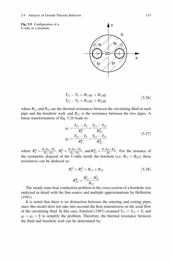
Fig. 5.9 Configuration of aU-tube in a borehole

Tf 1 � Tb ¼ R11q1 þ R12q2

Tf 2 � Tb ¼ R12q1 þ R22q2ð5:26Þ

where R11 and R22 are the thermal resistances between the circulating fluid in eachpipe and the borehole wall, and R12 is the resistance between the two pipes. Alinear transformation of Eq. 5.26 leads to:

q1 ¼Tf 1 � Tb

RD1

þ Tf 1 � Tf 2

RD12

q2 ¼Tf 2 � Tb

RD2

þ Tf 2 � Tf 1

RD12

ð5:27Þ

where RD1 ¼

R11R22�R212

R22�R12; RD

2 ¼R11R22�R2

12R11�R12

; and RD12 ¼

R11R22�R212

R12: For the instance of

the symmetric disposal of the U-tube inside the borehole (i.e. R11 ¼ R22), theseresistances can be deduced as:

RD1 ¼ RD

2 ¼ R11 þ R12 ð5:28Þ

RD12 ¼

R211 � R2

12

R12

The steady-state heat conduction problem in the cross-section of a borehole wasanalyzed in detail with the line-source and multiple approximations by Hellström(1991).

It is noted that there is no distinction between the entering and exiting pipessince this model does not take into account the heat transmission on the axial flowof the circulating fluid. In this case, Eskilson (1987) assumed Tf 1 ¼ Tf 2 ¼ Tf andq1 ¼ q2 ¼ ql

2 to simplify the problem. Therefore, the thermal resistance betweenthe fluid and borehole wall can be determined by:


Rb2 ¼R11 þ R12

2ð5:29Þ

With these assumptions, the temperatures of the fluid entering and exiting theGHE can be calculated. Being superior to the model of an equivalent pipe, thistwo-dimensional model presented quantitative expressions of the thermal resis-tance in the cross-section, and provided a basis for discussing the impact of the U-tube disposal on the heat conduction. However, the temperatures of the fluidcirculating through different legs of the U-tubes are, in fact, different. As a result,the thermal interference or thermal ‘‘short circuiting’’ between the U-tube legs isinevitable, which degrades the effective heat transfer in the GHEs. With theassumption of identical temperature of all the pipes, it is impossible for the two-dimensional model to reveal the impact of this thermal interference on the GHEperformance.

5.4.2.3 Quasi-Three-Dimensional Model

On the basis of the two-dimensional model aforementioned, a quasi-three-dimensional model was proposed by Zeng et al. (2003). The model takes accountof the fluid temperature variation along the borehole depth. Being minor in theorder, the conductive heat flow in the grout in axial direction, however, is stillneglected so as to keep the model concise and analytically manageable. Theenergy equilibrium equations can be written for upflow and downflow of thecirculating fluid:

�McdTf 1

dz¼ Tf 1 � Tb

RD1

þ Tf 1 � Tf 2

RD12

McdTf 2

dz¼ Tf 2 � Tb

RD2

þ Tf 2 � Tf 1

RD12

. . . 0� z�Hð Þð5:30Þ

Two conditions are necessary to complete the solution:

z ¼ 0; Tf 1 ¼ T 0f

z ¼ H; Tf 1 ¼ Tf 2

ð5:31Þ

The general solution to this problem is derived by Laplace transformation,which is slightly complicated in form. For the instance of the symmetric placementof the U-tube inside the borehole, the temperature profiles in the two pipes wereillustrated by Diao et al. (2004). For the purpose of practical applications an

alternative parameter e ¼ T 0f�T 00fT 00f �Tb

is derived from the temperature profiles, which is

named as the heat transfer efficiency of the borehole. It should be noticed thatT 0f and T00f and are the entering/exiting fluid temperatures to/from the U-tube.From the derived temperature profile, a more accurate heat conduction resistancebetween the fluid inside the U-tube and the borehole wall can be calculated by


Rb3 ¼H

Mc

1e� 1

2

ð5:32Þ

The authors validated that the quasi-three-dimensional model was more accu-rate than the other current models and recommended it for the design and thermalanalysis of the GHEs.

5.5 Current Status

The first field experiments for a BTES system occurred in 1976 in France, and thefirst large-scale system was brought online in 1982 near Luleå, Sweden. Thelargest BTES field in the world was built in 1995, consists of 400 boreholes with adepth of 135 m, and is located at Richard Stockton State College, Pomona, NewJersey, USA.

5.5.1 Sweden

Sweden is one of the leading countries in using the BTES for heating and cooling.Heat pumps are usually part of such systems that supplies about 20 % (20 TWh) ofall space heating in Sweden (Nordell et al. 2007). There are about 300,000 heatingsystems in operation for single-family houses, with an increase of 35–40,000systems, annually. During the last decade more than 1,000 larger systems havealso been constructed. These are usually for both heating and cooling though thereare large plants for heating only or cooling only. This energy efficient technologyis environmentally benign since extracted heat is renewable energy that is pas-sively stored from ground surface. These systems are most efficient if low-tem-perature heat distribution systems are used.

Heating systems by using the ground for heat extraction have been increasinglypopular during the last decades. Typical payoff times are 10–15 years but therising energy cost improves the economy considerably. Another fact is that thevalue of the house increases at least with the investment. For larger sys-tems [1,000–3,000 MWh the economy is considerably better with typical payofftimes of 2–6 years.

Large-scale BTES are mainly used for seasonal heat storage. Typical heat sourcesare industrial waste heat or solar heat. The most favorable system is high-temperaturestorage for low-temperature applications, where no heat pump or additional heatingis required. The solar system in Anneberg, Stockholm, is a good example of howsolar heat is stored and used for space heating. In this case, about 1,000 MWh is storedfrom the summer and used for heating of 60 single-family houses during the winter.Stored heat is used at a temperature of 32 �C, for heating of tap water and spaceheating through the low-temperature floor heat distribution system.


Storage temperatures up to about 80–90 �C are used in BTES though low-temperature systems are most common. Occurring heat losses from such systemsdepends on the bedrock properties, temperature, geometry, and volume. The firsthigh-temperature BTES (82 �C), with a volume of 120,000 m3, was constructed inLuleå, Sweden. Its heat loss was about 40 %. In larger (few hundred thousand m3)heat temperature BTES systems the annual loss is about 10–15 %.

5.5.2 Canada

Two systems have recently been developed in Canada. The first being NorthAmerica’s second largest field, built in 2004 at the University of Ontario Instituteof Technology. The field consists of 370 boreholes with a depth of 200 m,arranged in a 14 by 27 grid with 4.5 m spacing (Wong et al. 2006). Now, thethermal storage system is a critical component of the university’s heating andcooling system, and helps to keep the cost down and the efficiency up. In addition,the thermal storage system is used for research and to educate students in TES.Researchers and students have the rich opportunity of on-site research and edu-cation in one of North America’s biggest geothermal fields (Gao et al. 2009).

The second Canadian example is the 52-house Solar Community, in OkotoksAlberta. This project uses both a BTES field and two above-groundwater thermalstorage tanks. The solar BTES residential development is located in a newdevelopment called the Drake Landing community. The new subdivision to beheated by an integrated solar and BTES system consists of 52 single-family homeseach with floor space in the range of 1,400–1,600 square foot. Systems relying onthermal resources having significant short-term variations such as solar thermalusually combine the larger seasonal storage system with a smaller water-filledbuffer tank to increase short-term response. The borehole field consists of 144boreholes, each 35 m deep with 150 mm diameter, with 2.25 m spacing. Thesystem contains 24 parallel circuits, each having six boreholes in series. Thissystem saves more than 110 GJ of energy, and five tons of GHGs per homeannually, and has a solar fraction (percentage of energy use that is met by solargains) of nearly 90 % (Wong et al. 2006). These examples show that BTESsystems are feasible for a large range of project types and settings.

5.5.3 Belgium

BTES applications are an alternative solution for regions where ATES applicationscannot be applied due to the absence of an aquifer and are normally used in small-scale applications in the commercial sector such as hospitals, office buildings, etc.,for cooling and heating. According to Desmedt et al. (2006), there is large interestin BTES applications in recent years. VITO carried out several feasibility studies


in the health and commercial building sector on ground-source heat pumps(GSHP) in combination with vertical borehole heat exchangers (BHEs). A numberof these feasibility studies have resulted in concrete projects. The easy way ofinstalling and operating the BTES in conjunction with ATES applications has animportant impact on this evolution. BTES applications are most suitable for sea-sonable thermal storage such as solar heat, heat from cogeneration units duringsummer period, etc., and are a proved technology to work without any leaks orcollapses. One other advantage of these applications is that the system can be usedfor direct or natural cooling during summer period (without the need for a classicalmechanical chiller consuming a lot of electricity), on one condition that the airhanding units (AHUs) are suitable and designed for the higher temperature levels(e.g. 14/18 �C instead of 6/12 �C for cooling purposes). This natural cooling canbe delivered at a high COP (coefficient of performance) and by regenerating theground this delivers an improved heat pump operation in winter period. Undernormal conditions, small-scale BTES applications for combined heating andcooling commonly will be paid back within 7–10 years.

During winter the high-temperature heat (radiators) is produced by gas-firedboilers and the low-temperature heat (AHUs, floor heating) by the heat pump. Ifthe heat from the heat pump is insufficient the gas-fired boilers can support them.The heat pump is designed for a part of the low-temperature heat demand becausethe BHE’s cannot deliver the whole needed evaporator heat. The number of BHE’sis determined on an economic optimum.

During summer period (only cooling) the BHE’s deliver direct or naturalcooling at a temperature level of 14/18 �C. If the cooling demand is higher thanthe limit of the BHEs, the reversible heat pump and/or the classical chiller candeliver the extra cooling.

Most of the BTES applications are situated in hospitals and office buildingswhere of course ATES was not possible for the location. The typical heating andcooling capacity is 25–650 kW using 10–250 boreholes 30–150 m in depth.Typical layers consist mainly of sand or sand and clay.

When designing BHEs with GSHPs the knowledge of ground thermal proper-ties (thermal conductivity, borehole thermal resistance, undisturbed soil temper-ature, specific heat capacity, etc.) are important for correct functioning of thesystem. Due to the higher investments costs, oversizing of BHEs and GSHPs paysa higher penalty than in conventional applications. Obtaining accurate values forthermal ground properties requires detailed survey on site by a thermal responsetest. Parameters that can have an influence on the result are the building load,borehole spacing, borehole fill material, and the on-site characteristics. In the lastyear, there was a growing interest in thermal response tests. In situ testing hasrecently become a standard measurement for larger BTES applications.

However, the data obtained from a thermal response test is useless data forengineering companies. The reason why BTES application are nowadays notcommon practice is the lack of technical knowledge from engineering companies,no financial incentives for the technology, extra investments costs, no believe inthe proven BTES technology, etc. Most of the engineering companies and building

5.5 Current Status 119

owners find that the integration of BHEs and GSHPs can be simplified by somerules of thumb as they are used for calculating the heating and cooling demand ofbuildings. The opposite is true. When designing new buildings the owner appointsan engineering company that must know every innovative technique that isavailable in the sector. This is impossible for small engineering companies due tolack of personnel. The building sector in Belgium has to search for advice byenergy consulting companies when designing new buildings. This needs a changein mentality which can not be solved in a few years and needs the cooperation ofseveral actors in the building sector.

5.5.4 Germany

Mangold (2007), Mangold and Schmidt (2009), and Nubbicker-Lux et al. (2009)reported the history and current status of BTES in Germany. Since 1997 a pilotborehole thermal energy storage is in realization in Neckarsulm. In the first step,the feasibility of the storage concept was proven with the installation of a 5,000 m3

research storage at the site of the plant. The ducts are double-U-pipes made ofpolybutene with a depth of 30 m. The design data of the model calculations havebeen validated by the experimental results of the monitoring program. In 1999, thestorage was enlarged to a storage volume of 20,000 m3. In 2002, the next phase ofthe solar assisted district heating project was started: the borehole storage wasenlarged to 63,300 m3 storage volume reaching half of the finally planned volume.The BTES is directly connected to the heat distribution network and charged bythe solar collectors by means of two 100 m3 buffer tanks. The two buffer tanks areused for short-term heat storage to balance peaks in heat delivery from the solarcollectors. The buildings are connected to the district heating system via a 3-pipeheat distribution network. The heat distribution network is supplied either by thebuffer tanks or the BTES, depending on the temperature level. A condensing gasboiler supplies additional heat to provide the required temperature level.

Next generation borehole thermal energy storage was built in Crailsheim in2008. The storage consists of 80 boreholes with a depth of 55 m in a first con-struction phase. The storage volume (37,500 m3) is a cylinder with the boreholessituated in a 3 9 3 m square pattern. The ground heat exchangers are double-U-pipes made from cross-linked polyethylene (PEX). The storage volume will bedoubled when the second part of the connected residential area is going to be builtin some years.

The hydro-geological investigation showed an intermittent water movement inthe upper part (5 m) of the storage volume. For this reason, the boreholes weredrilled with a bigger diameter in this part. After installation of the ground heatexchangers the lower part was filled with a thermally enhanced grouting material(thermal conductivity 2.0 W/mK), whereas the upper part was filled with a ther-mally reduced grouting material to reduce the heat transfer into this layer andthereby the thermal losses due to the water movement in this region. The


horizontal piping on top of the storage is embedded into an insulation layer offoam glass gravel. On top of the insulation layer a protecting foil (water-tight butopen for vapor diffusion) and a drainage layer (gravel) are installed below a 2 mlayer of soil.

5.5.5 Switzerland

In Switzerland, geothermal heat pump systems have found a high level of popu-larity for space heating purposes and deliver in total an annual geothermal energyof * 1 TWh (Signorelli 2004). Actual statistical evaluations show that in Swit-zerland [50 % of geothermal energy is produced by borehole heat exchangers(BHEs).

Since BHE heating systems mainly use the temperature field below a depth of20 m, which is not influenced by atmospheric conditions or seasonal variability,they always achieve a high efficiency even when the ambient air temperature islow. For BHE-coupled heat pumps COP values are generally higher than 4. Thisfact has contributed to the high popularity of BHE systems in Switzerland. Since1980 over 30,000 buildings have been heated by BHE systems, corresponding to4,700 km of drilled BHEs. Most BHE systems are located in the Alpine Foreland,the most densely populated area. In terms of areal density (BHE/km2), Switzerlandis the world leader in this ecologically friendly technology.

5.5.6 Norway

Today, the most frequently used energy storage technology for heat and cold isUnderground Thermal Energy Storage (UTES) systems combined with Ground-Source Heat Pumps (GSHP). The Norwegian geology favors Borehole ThermalEnergy Storage (BTES) applications and at present time the number of BTESinstallations is about 90 (Midttømme et al. 2009).

An example of a standard BTES has recently been completed at Falstadsenteret,a 2,850 m2 historical museum in Levanger. The heating and cooling systemcomprises a 130 kW heat pump and thirteen 180 m deep Borehole HeatExchangers (BHE). The total cost of the GSHP and BTES is 170,000 Euro, and thepayback time compared to conventional heating and cooling systems is estimatedto be 12 years. Some of the largest BTES systems in Europe are located in Norwayas indicated in Table 5.1.

A BTES system comprising 228 boreholes of 200 m depth was drilled duringwinter 2007, and will provide heat and cold to the new Akershus UniversityHospital (Ahus). The building has a total floor area of 137,000 m2, and an annualheating and cooling demand of 26 GWh and 8 GWh, respectively. One of the goals


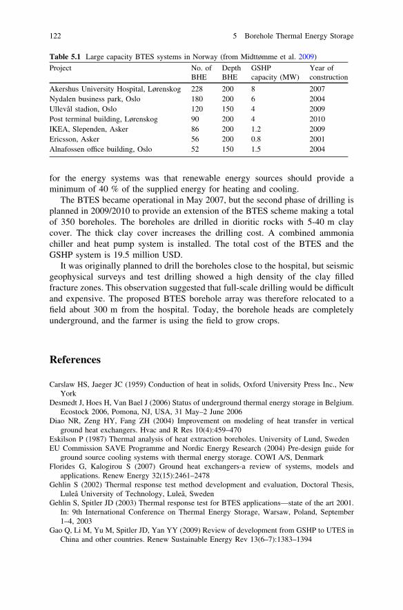
for the energy systems was that renewable energy sources should provide aminimum of 40 % of the supplied energy for heating and cooling.

The BTES became operational in May 2007, but the second phase of drilling isplanned in 2009/2010 to provide an extension of the BTES scheme making a totalof 350 boreholes. The boreholes are drilled in dioritic rocks with 5-40 m claycover. The thick clay cover increases the drilling cost. A combined ammoniachiller and heat pump system is installed. The total cost of the BTES and theGSHP system is 19.5 million USD.

It was originally planned to drill the boreholes close to the hospital, but seismicgeophysical surveys and test drilling showed a high density of the clay filledfracture zones. This observation suggested that full-scale drilling would be difficultand expensive. The proposed BTES borehole array was therefore relocated to afield about 300 m from the hospital. Today, the borehole heads are completelyunderground, and the farmer is using the field to grow crops.

References

Carslaw HS, Jaeger JC (1959) Conduction of heat in solids, Oxford University Press Inc., NewYork

Desmedt J, Hoes H, Van Bael J (2006) Status of underground thermal energy storage in Belgium.Ecostock 2006, Pomona, NJ, USA, 31 May–2 June 2006

Diao NR, Zeng HY, Fang ZH (2004) Improvement on modeling of heat transfer in verticalground heat exchangers. Hvac and R Res 10(4):459–470

Eskilson P (1987) Thermal analysis of heat extraction boreholes. University of Lund, SwedenEU Commission SAVE Programme and Nordic Energy Research (2004) Pre-design guide for

ground source cooling systems with thermal energy storage. COWI A/S, DenmarkFlorides G, Kalogirou S (2007) Ground heat exchangers-a review of systems, models and

applications. Renew Energy 32(15):2461–2478Gehlin S (2002) Thermal response test method development and evaluation, Doctoral Thesis,

Luleå University of Technology, Luleå, SwedenGehlin S, Spitler JD (2003) Thermal response test for BTES applications—state of the art 2001.

In: 9th International Conference on Thermal Energy Storage, Warsaw, Poland, September1–4, 2003

Gao Q, Li M, Yu M, Spitler JD, Yan YY (2009) Review of development from GSHP to UTES inChina and other countries. Renew Sustainable Energy Rev 13(6–7):1383–1394

Table 5.1 Large capacity BTES systems in Norway (from Midttømme et al. 2009)

Project No. ofBHE

DepthBHE

GSHPcapacity (MW)

Year ofconstruction

Akershus University Hospital, Lørenskog 228 200 8 2007Nydalen business park, Oslo 180 200 6 2004Ullevål stadion, Oslo 120 150 4 2009Post terminal building, Lørenskog 90 200 4 2010IKEA, Slependen, Asker 86 200 1.2 2009Ericsson, Asker 56 200 0.8 2001Alnafossen office building, Oslo 52 150 1.5 2004


Gu Y, O’Neal DL (1998) Development of an equivalent diameter expression for vertical U-tubesused in ground-coupled heat pumps. ASHRAE Transactions 104(2):347–355

He MM (2007) Analysis of underground thermal energy storage systems with ground wateradvection in subtropical regions, Master’s Thesis, The University of Hong Kong, Hong Kong

Hellström G (1991) Ground heat storage: thermal analyses of duct storage systems. University ofLund, Sweden

http://www.dlsc.ca/borehole.htmhttp://underground-energy.com/BTES.htmlIngersoll LR, Zobel OJ, Ingersoll AC (1954) Heat conduction with engineering, geological, and

other applications, McGraw-Hill, New YorkInternational energy Agency (2006) Energy conservation through energy storage programmeMangold D (2007) Seasonal storage—a German success story. Sun & Wind Energy 1:48–58Mangold D., Schmidt T (2009) The next generations of seasonal thermal energy storage in

Germany. ESTEC 2009, Munich, Germany, May 25–26Midttømme K, Hauge A, Grini RS, Stene J, Skarphagen H (2009) Underground thermal energy

storage (UTES) with heat pumps in Norway. In: Proceedings of Effstock 2009, Stockholm,Sweden, June 15–17, 2009

Nielsen K (2003) Thermal energy storage. A state-of-the-art, NTNU, TrondheimNordell B (2000) Large-scale thermal energy storage. WinterCities’2000, Energy and Environ-

ment, Luleå, Sweden, Feb 14, 2000Nordell B, Grein M, Kharseh M (2007) Large-scale utilisation of renewable energy requires

energy storage. In: International Conference for Renewable Energies and SustainableDevelopment (ICRESD_07), Université Abou Bakr BELKAID – TLEMCEN, Algeria, May21–24, 2007

Nubbicker-Lux J, Heidemann W, Müller-Steinhagen H (2009) Validation of a computer modelfor solar coupled district heating systems with borehole thermal energy storage. EFFSTOCK2009, Stockholm, Sweden, June 14–17, 2009

Sannera B, Karytsasb C, Mendrinosb D, Rybachc L (2003) Current status of ground source heatpumps and underground thermal energy storage in Europe. Geothermics 32(4–6):579–588

Signorelli S (2004) Geoscientific investigations for the use of shallow low-enthalpy system. Sc.D.dissertation, Swiss Federal Institute of Technology, Zurich

Wong B, Snijders A, McClung L (2006) Recent inter-seasonal underground thermal energystorage applications in Canada. EIC Climate Change Technology, 2006 IEEE, Ottawa, ON,May 10–12, 2006

Yang H, Cui P, Fang Z (2010) Vertical-borehole ground-coupled heat pumps: a review of modelsand systems. Appl Energy 87(1):16–27

Yavuzturk C (1999) Modeling of vertical ground loop heat exchangers for ground source heatpump systems, Oklahoma State University, Stillwater

Zeng HY, Diao NR, Fang ZH (2003) Heat transfer analysis of boreholes in vertical ground heatexchangers. Heat and Mass Transf 46(23):4467–4481

Zizzo R (2009) Designing an optimal urban community mix for an aquifer thermal energy storagesystem, M.S. Thesis, University of Toronto, Toronto

References 123



Chapter 6Cavern Thermal Energy Storage Systems

6.1 Introduction

Cavern thermal energy storage (CTES) belongs to the seasonal sensible liquidstorage in various forms of underground cavities (EU Commission SAVE Pro-gramme and Nordic Energy Research 2004). Potential structures for CTES includeabandoned mines, tunnels or rock caverns, natural karst structures, and artificiallyconstructed caverns in rock or deep pits in soil. For artificial caverns, CTES needsconstruction of large underground water reservoirs to serve as the thermal energysystem. Enormous investment for the construction limits the practical applicationof the cavern storage method, which is seldom used nowadays.

When warm/hot water is first filled into the cavern, the heat losses to thesurrounding rock mass will be substantial. However, during the first year or twoafter charging, the cavern develops a relatively stable thermal halo around itselfwith decreasing temperature away from the warm/hot center. There will still be aloss of heat, but dry rock is generally a poor heat conductor. The heat loss shouldbe less than 10 % during one operational cycle under favorable conditions.A crucial factor is groundwater transport through the rock masses in the area, theless the better.

The advantage of rock cavern heat storage includes very high injection andextraction powers (just a matter of pump capacity), while the disadvantage is itshigh construction cost. There are some examples of how old rock caverns,previously used for oil storage, have been converted for high temperature waterstorage (Nordell et al. 2007).

In the rock CTES, energy is stored as hot water in an underground cavern. Insuch a system with a large volume of water it is of great importance to maintain astratified temperature profile in the cavern. During injection hot water is injected atthe top of the store while colder water is extracted from the bottom.


125

6.2 Analysis

Rehbinder and Reichelt (1984) considered the quasi-steady solution of the heatconduction equation for this geometry with periodic temperature variations. Theanalysis is based upon a number of simplifications and assumptions. They alsoassumed that the convection of heat with the groundwater can be neglected.The density and heat capacity of the rock are constants and the heat conductioncoefficient is isotropic and constant. The cavern is a torus with cylindrical symmetry.The cavern is assumed to be located well below the ground, implying that the presenceof a free ground surface can be neglected. The first assumptions, dealing with the rockproperties, are reasonable; for economic reasons the cavern has been located in verygood quality rock. The shape of the cavern is not perfectly symmetrical but thedeviation is small. The last assumption, that the ground surface has no influence, is themost questionable since the distance between the top and bottom of the cavern is equalto the distance between the top of the cavern and the ground surface.

Consider a region exterior to a torus X symmetric with respect to the z-axis,with the boundary qX. Let the inner radius of qX be the characteristic length of theproblem (Fig. 6.1). At qX the temperature T is prescribed ToU r; tð Þ where theconstant To is the characteristic temperature of the problem, and U r; tð Þ is a givenfunction of 0;1½ Þ � oX. The temperature is assumed to vanish at infinity. Theinitial temperature is zero. The region consists of a rock whose heat conduction isk, heat capacity C, and density q. These parameters can be combined giving thediffusivity a ¼ k

qC. Thus with cylindrical coordinates:

oT

ot¼ a

o2T

or2þ 1

r

oT

orþ o2T

oz2

� �in X ð6:1Þ

T r; z; tð Þ ¼ ToU t; rð Þ on oX t � 0

T r; z; tð Þ ¼ 0 r2 þ z2 !1 t [ 0

T r; z; tð Þ ¼ 0 in X t \ 0

The solution can be expressed with the T-matrix representation used in scat-tering theory. To solve the limiting problem u t; rð Þ ¼ exp ixtð Þ when t! 0, thefollowing variables are introduced.

u ¼ Te�ixt

Toð6:2Þ

n ¼ r

a

f ¼ z

a

s ¼ at

a2

126 6 Cavern Thermal Energy Storage Systems

b ¼ b

a

h ¼ h

a

x ¼ xa2

a

k ¼ e

3pi

4 x12

The heat conduction problem above is then reduced to a boundary valueproblem for the Helmholtz equation. The parameters a, b, and h can be varied tostudy their effect on u. Helmholtz problem in cylindrical coordinates is:

o2u

on2 þ1n

ou

onþ o2u

of2 þ k2u ¼ 0 in X ð6:3Þ

u ¼ 1 on oX

limR!1

Rou

oR� iku

� �¼ 0 R ¼

ffiffiffiffiffiffiffiffiffiffiffiffiffiffiffin2 þ f2

q

Rehbinder and Reichelt (1984) sought the solution in the form of a linearcombination of particular solutions, which satisfy Eq. 6.3. By using cylindricallysymmetric particular solutions, it can be shown that the cylindrically symmetricthree-dimensional problem on an infinite domain is reduced to a one-dimensionalapproximation problem on a curve of finite length.

If h� 1, the solution of Eq. 6.3 in the vicinity of f ¼ 0 is equal to the solutionsfor pure radial flow. These solutions can be found in Carslaw and Jaeger (1959)’stextbook.

Fig. 6.1 The torus region

6.2 Analysis 127

u ¼ K0 knð ÞK0 kb� � n� b kj j[ 0

u ¼ I0 knð ÞI0 kð Þ n� 1

The modified Bessel functions Kv, and Iv, for a complex argument are mostconveniently expressed with the modulii Mv, and Nv, and phases hv and uv, ofKelvin’s functions. Then, the solutions can be in simple form:

u nð Þ ¼N0 n

ffiffiffiffixp� �

N0 bffiffiffiffixp� � ei /0 n

ffiffiffixpð Þ�/0 b

ffiffiffixpð Þ½ � n� b

u nð Þ ¼M0 n

ffiffiffiffixp� �

M0 bffiffiffiffixp� � ei /0 n

ffiffiffixpð Þ�/0 b

ffiffiffixpð Þ½ � n� 1

6.3 Current Status

Two CTES systems were built in Sweden, Avesta with a volume of 15,000 m3 andLyckebo with a storage volume of 115,000 m3. The Avesta CTES was built in1981 for short-term storage of heat produced at an incineration plant. The Lyckebostore, which is partly heated by solar energy, has been in operation since 1983. Thestorage volume of 115,000 m3 had a maximum water temperature of 90 �C and5,500 MWh of heat was stored between the seasons (Nordell et al. 2007). Therewere a few more CTES systems built but in these cases the caverns used were notinitially constructed for CTES. There are examples of shut down mines and oilstorage caverns that have been reconstructed for hot water storage.

For the time being, there are no CTES applications for storage of cold incaverns. However, storage of snow (or ice) in pits is a promising storage concept.One such demonstration project has been realized in Sundsvall, Sweden. Here, asnow pit supplies some 2 MW of comfort cooling to a hospital, as shown inFig. 6.2 (EU Commission SAVE Programme and Nordic Energy Research 2004).

The snow melted by heat transfer from the surroundings is called naturalmelting, and it depends on climate, area of the storage, and insulation. In theSundsvall case, the pit is only a couple of meters deep, and to prevent the naturalmelting, the snow layer is insulated with wood chips. In this case, the predictednatural melt is about 20–25 % of the 30,000 m3 snow pile. Cold can be extractedeither by putting pipes under the snow pile and circulating a heat carrier, or bycirculating the melted water itself. In Sundsvall, the melt water circulation solutionis used.

128 6 Cavern Thermal Energy Storage Systems

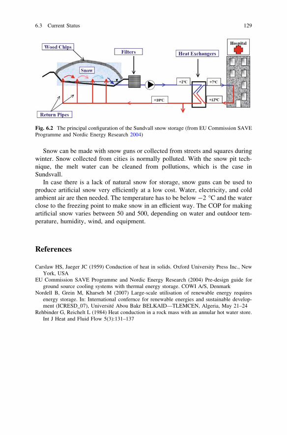
Snow can be made with snow guns or collected from streets and squares duringwinter. Snow collected from cities is normally polluted. With the snow pit tech-nique, the melt water can be cleaned from pollutions, which is the case inSundsvall.

In case there is a lack of natural snow for storage, snow guns can be used toproduce artificial snow very efficiently at a low cost. Water, electricity, and coldambient air are then needed. The temperature has to be below -2 �C and the waterclose to the freezing point to make snow in an efficient way. The COP for makingartificial snow varies between 50 and 500, depending on water and outdoor tem-perature, humidity, wind, and equipment.

References

Carslaw HS, Jaeger JC (1959) Conduction of heat in solids. Oxford University Press Inc., NewYork, USA


Nordell B, Grein M, Kharseh M (2007) Large-scale utilisation of renewable energy requiresenergy storage. In: International confernce for renewable energies and sustainable develop-ment (ICRESD_07), Université Abou Bakr BELKAID—TLEMCEN, Algeria, May 21–24

Rehbinder G, Reichelt L (1984) Heat conduction in a rock mass with an annular hot water store.Int J Heat and Fluid Flow 5(3):131–137

Fig. 6.2 The principal configuration of the Sundvall snow storage (from EU Commission SAVEProgramme and Nordic Energy Research 2004)


Chapter 7Standing Column Well

7.1 Definition

A number of ground systems cannot be categorized either as open or as closed.Such a system is the standing column well (SCW) shown in Fig. 7.1, where wateris pumped from the bottom of the well to the heat pump (Florides and Kalogirou2007). The exiting water is percolated through gravel in the annulus of the well inorder to absorb heat. Standing wells are typically 15 cm in diameter and may be asdeep as 500 m.

In his chapter, Deng (2004) provided an excellent review on SCW and thischapter is mainly based on his work. SCW systems are also referred to in theliterature as ‘‘turbulent wells’’, ‘‘energy wells’’, ‘‘concentric wells’’, ‘‘recirculatingwells’’, ‘‘geo-wells’’, ‘‘thermal wells’’, and ‘‘closed-loop, open-pipe systems’’.

The use of SCW was first suggested by local Maine well drillers and hydrog-eologists. In fact, the concept of SCW systems is about as old as the groundwaterheat pump systems, but is recently receiving much more attention because of theirlower installation cost, lower operating cost, and improved overall performance inthe regions with suitable geological conditions.

Compared to other ground heat source heat pump systems, shorter boreholesand more stable water temperatures make the SCW system an attractive com-mercial and industrial design approach. Now, there are approximately 1,000 SCWinstallations in the United States. Most of them are located in the Northeast andPacific Northwest in addition to parts of Canada in heating-dominated residentialand light commercial applications. These regions have lower mean ground tem-perature and higher heating loads than other areas, so now most SCW design isfocused on heat extraction.


131

7.2 Operation

The SCW system can be considered as a cross between closed-loop earth-coupledsystem and open-loop groundwater source system. During much of the year, theyare operated by recirculating water between the well and the heat pump. However,during peak temperature periods, they can ‘‘bleed’’ some water from the system toinduce groundwater flow. The SCW systems adopted various numbers of wellsdepending on system capacity. Usually, only one well is required. Larger projectsmay have several wells in parallel.

In SCW systems, water is recirculated between the well and the building (heatpump). Deep bores are drilled in hard rock, creating a standing column of waterfrom the static water level down to the bottom of the bore. Water is recirculatedfrom one end of the column to the heat pump, and back to the other end of thecolumn (Fig. 7.2).

During peak heat rejection or extraction periods, if the well-water temperaturedrops too low or climbs too high, SCW systems can bleed part of the water ratherthan returning it all to the well. This causes water to flow to the column from thesurrounding formation to make up the flow. This cools the column and surroundingground during heat rejection in the summer, and heats the column and surroundingground during heat extraction in the winter. This flow thus restores the well-watertemperature to the normal operating range and improves the system performance.The bleed water can be diverted to a storm sewer, used for domestic water

Fig. 7.1 Standing column well (from Florides and Kalogirou 2007)

132 7 Standing Column Well

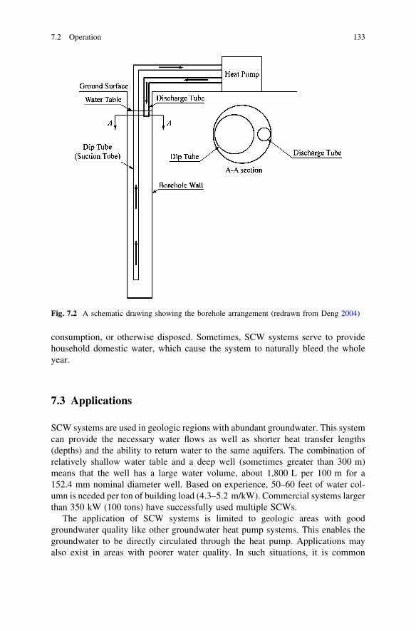
consumption, or otherwise disposed. Sometimes, SCW systems serve to providehousehold domestic water, which cause the system to naturally bleed the wholeyear.

7.3 Applications

SCW systems are used in geologic regions with abundant groundwater. This systemcan provide the necessary water flows as well as shorter heat transfer lengths(depths) and the ability to return water to the same aquifers. The combination ofrelatively shallow water table and a deep well (sometimes greater than 300 m)means that the well has a large water volume, about 1,800 L per 100 m for a152.4 mm nominal diameter well. Based on experience, 50–60 feet of water col-umn is needed per ton of building load (4.3–5.2 m/kW). Commercial systems largerthan 350 kW (100 tons) have successfully used multiple SCWs.

The application of SCW systems is limited to geologic areas with goodgroundwater quality like other groundwater heat pump systems. This enables thegroundwater to be directly circulated through the heat pump. Applications mayalso exist in areas with poorer water quality. In such situations, it is common

Fig. 7.2 A schematic drawing showing the borehole arrangement (redrawn from Deng 2004)

7.2 Operation 133

practice to use an intermediate heat exchanger between the well and the heat pumpin order to avoid fouling the heat pump heat exchangers.

It is suggested that the designer of SCW systems should (1) work with anexperienced local hydrologist and (2) avoid any areas with salt bed or otherformation that could be dissolved. Also, any water well including SCWs must beconstructed, developed, and operated according to state and local regulations forwater wells. It is imperative that designers and installers of SCW systems be awareof the regulations in their locations.

SCW systems have some advantages shared with all the other forms of groundsource heat pump systems:

• Economy

When properly designed, a geothermal heat pump system is one of the lowestcost ways of providing heating/cooling because of high equipment efficiency,annual storage/reuse of energy, and availability. However, geothermal heat pumpsystems have comparatively high capital costs. A geothermal system often haslower life cycle costs than conventional systems due to its reduced energy andmaintenance costs. Because there is no outdoor equipment in the geothermalsystems, corrosion, weathering, and vandalism are not normal problems.

• Environmental benefits

The need for electricity (pumps) introduces the only credible source of possibleenvironmental concern for a geothermal system. The geothermal system itselfproduces zero local pollution. This system causes less carbon dioxide emission andother pollutants than its conventional alternatives, thus reducing global warmingand other environmental impacts.

• Reduced requirement for mechanical room floor place• Quiet operation• Potential for reducing the peak electrical demand

Standing column well systems share the same advantages, in terms of energyefficiency, environmental benefits, low maintenance, etc., with other forms ofgeothermal heat pump systems. At the same time, the heat exchange rate in a SCWis enhanced by direct contact and by the pumping action, which promotesgroundwater flow to and from the borehole. Consequently, heat transfer with thesurrounding rock takes place by advection in addition to conduction. If a SCW isconsidered as a cylinder, the surface area for heat exchange of a 152.4 mmborehole with 304 m long is about 145 m2, which allows substantial heatexchange. Putting another way, SCW systems have substantially heat exchangerate and the fact that such systems are open loop means that the fluid flowingthrough the heat pump system is closer to the mean ground temperature comparedto systems with closed-loop U-tube heat exchangers.

SCW systems have a lower initial cost because the borehole depths are in the50–60 feet per ton compared to closed loops at 150 or more feet per ton. Thus, the


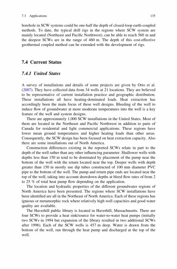
borehole in SCW systems could be one-half the depth of closed-loop earth-coupledmethods. To date, the typical drill rigs in the regions where SCW system aremainly located (Northeast and Pacific Northwest), can be able to reach 560 m andthe deepest SCWs are in the range of 460 m. The depth of this cost-effectivegeothermal coupled method can be extended with the development of rigs.

7.4 Current Status

7.4.1 United States

A survey of installations and details of some projects are given by Orio et al.(2007). They have collected data from 34 wells at 21 locations. They are believedto be representative of current installation practice and geographic distribution.These installations all have heating-dominated loads. Heat extraction hasaccordingly been the main focus of these well designs. Bleeding of the well toinduce flow of groundwater at more moderate temperatures into the well is a keyfeature of the well and system designs.

There are approximately 1,000 SCW installations in the United States. Most ofthem are located in the Northeast and Pacific Northwest in addition to parts ofCanada for residential and light commercial applications. These regions havelower mean ground temperatures and higher heating loads than other areas.Consequently, the SCW design has been focused on heat extraction capacity. Alsothere are some installations out of North America.

Construction differences existing in the reported SCWs relate in part to thedepth of the well rather than any other influencing parameter. Shallower wells withdepths less than 150 m tend to be dominated by placement of the pump near thebottom of the well with the return located near the top. Deeper wells with depthgreater than 150 m mostly use dip tubes constructed of 100 mm diameter PVCpipe to the bottom of the well. The pump and return pipe ends are located near thetop of the well, taking into account drawdown depths at bleed flow rates of from 2to 25 % of total heat pump flow depending on the application.

The location and hydraulic properties of the different groundwater regions ofNorth America have been presented. The regions where SCW installations havebeen identified are all in the Northeast of North America. Each of these regions hasigneous or metamorphic rock where relatively high well capacities and good waterquality are available.

The Haverhill public library is located in Haverhill, Massachusetts. There arefour SCWs to provide a heat sink/source for water-to-water heat pumps (initiallytwo SCWs in 1994 but expansion of the library resulted in two additional SCWsafter 1996). Each of the SCW wells is 457 m deep. Water is drawn from thebottom of the well, run through the heat pump and discharged at the top of thewell.

7.3 Applications 135

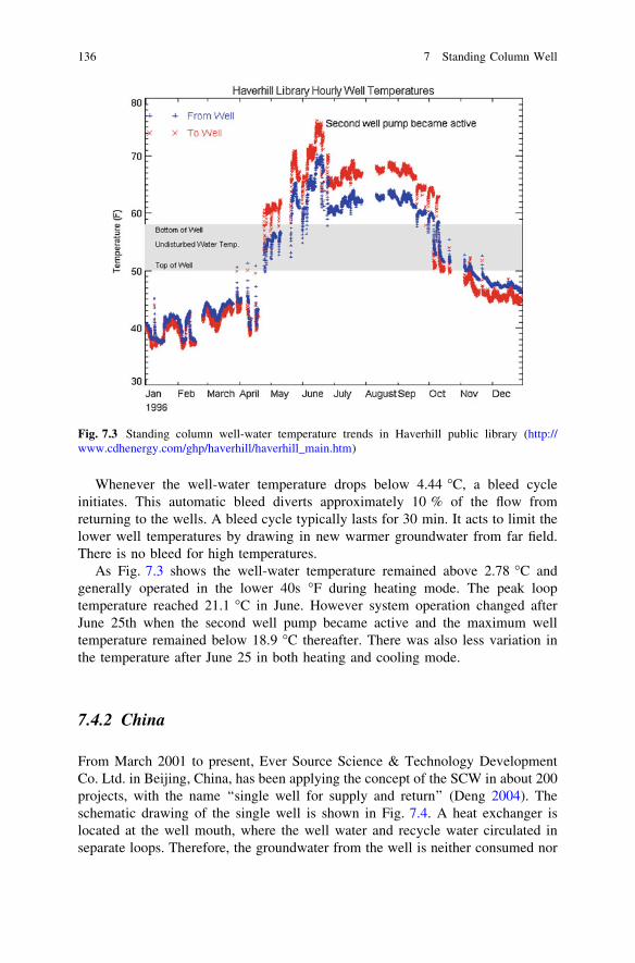
Whenever the well-water temperature drops below 4.44 �C, a bleed cycleinitiates. This automatic bleed diverts approximately 10 % of the flow fromreturning to the wells. A bleed cycle typically lasts for 30 min. It acts to limit thelower well temperatures by drawing in new warmer groundwater from far field.There is no bleed for high temperatures.

As Fig. 7.3 shows the well-water temperature remained above 2.78 �C andgenerally operated in the lower 40s �F during heating mode. The peak looptemperature reached 21.1 �C in June. However system operation changed afterJune 25th when the second well pump became active and the maximum welltemperature remained below 18.9 �C thereafter. There was also less variation inthe temperature after June 25 in both heating and cooling mode.

7.4.2 China

From March 2001 to present, Ever Source Science & Technology DevelopmentCo. Ltd. in Beijing, China, has been applying the concept of the SCW in about 200projects, with the name ‘‘single well for supply and return’’ (Deng 2004). Theschematic drawing of the single well is shown in Fig. 7.4. A heat exchanger islocated at the well mouth, where the well water and recycle water circulated inseparate loops. Therefore, the groundwater from the well is neither consumed nor

Fig. 7.3 Standing column well-water temperature trends in Haverhill public library (http://www.cdhenergy.com/ghp/haverhill/haverhill_main.htm)


http://www.cdhenergy.com/ghp/haverhill/haverhill_main.htm


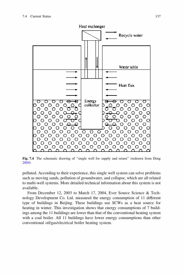
polluted. According to their experience, this single well system can solve problemssuch as moving sands, pollution of groundwater, and collapse, which are all relatedto multi-well systems. More detailed technical information about this system is notavailable.

From December 12, 2003 to March 17, 2004, Ever Source Science & Tech-nology Development Co. Ltd. measured the energy consumption of 11 differenttype of buildings in Beijing. These buildings use SCWs as a heat source forheating in winter. This investigation shows that energy consumptions of 7 build-ings among the 11 buildings are lower than that of the conventional heating systemwith a coal boiler. All 11 buildings have lower energy consumptions than otherconventional oil/gas/electrical boiler heating system.

Fig. 7.4 The schematic drawing of ‘‘single well for supply and return’’ (redrawn from Deng2004)


7.4.3 Korea

According to Lee (2009), 31 SCW systems were reported in Korea. Most of thegroundwater wells (74.2 %) in the SCW system were installed at depths of300–500 m with a mean of 391 m. It is considered that deeper wells in Korea arenecessary due to the installation of SCW systems in public and education buildingsthat have larger system capacities.

The SCW systems adopted various numbers of wells depending on systemcapacity. The number of groundwater wells ranged between 1 and 12 with a meanof 4.4 wells for each system. Similarly, with SCW systems in North America, welldiameters were generally 150 mm in bedrock with 200 mm steel casing from theground surface to the interface between upper soil and lower bedrock.

The installation cost of SCW systems depends mainly on system capacity. Forthe period of 2003–2006, the installation costs of SCW system (1055 kW) was$1,164,000. Meanwhile, the installation cost per unit capacity gradually decreasedwith years. The decease in the cost appears to be derived from the progress ofinstallation technology, and award competition in the market between geothermalcompanies. In 2008, the authority (Korea Energy Management Corporation)revised the recommended unit costs to $3,552/usRT for SCW systems.

References

Deng Z (2004) Modeling of standing column wells in ground source heat pump systems. PhDdissertation, Oklahoma State University, Stillwater, OK, USA

Florides G, Kalogirou S (2007) Ground heat exchangers—a review of systems, models andapplications. Renew Energy 32(15):2461–2478

http://www.cdhenergy.com/ghp/haverhill/haverhill_main.htmLee J-Y (2009) Current status of ground source heat pumps in Korea. Renew Sustain Energy Rev

13:1560–1568Orio CD, Johnson CN, Rees SJ, Chiasson A, Deng Z, Spitler JD (2007) A survey of standing

column well installations in North America. ASHRAE Trans 111(2):109–121



Chapter 8Modeling

8.1 General Aspects of Modeling

Performance of TES is influenced by various factors such as location, constructiontype, size, geometry, storage medium, and used materials. Furthermore, TES areintegrated in heating and cooling systems with a great variety of system configu-rations and control and operation strategies. Boundary conditions also influence theenergetic and exergetic efficiency of TES. Hence, for a realistic comparison systemsimulations are required, which include all sensitive parameters (Ochs et al. 2009).

The comparison of different (seasonal) TES is difficult. Comparing differenttypes of TES (ATES, BTES, tank, pit) without consideration of the entire energysystem (including production, distribution and load) may lead to wrong conclu-sions. The following parameters have to be considered.

• The volume and geometry of the TES, the design of the composite wall (concrete,insulation, and liner), the distribution of insulation (cover, side wall, and bottom),the insulation thickness and type may differ. The geometry (e.g. cuboid, cylinder,or cone) influences both the surface-to-volume-ratio which determines thethermal losses and the height-to-diameter ratio which influences the quality ofthermal stratification.

• The location may affect performance. For example, thermal losses depend onthe ambient and soil temperature and on soil properties, in particular the thermalconductivity and the volumetric heat capacity. At locations with groundwater,with or without regional groundwater flow, thermal losses are higher.

• The operational conditions such as the (average and maximum/minimum)operation temperatures, the return flow temperature of the heating net, or thenumber of charging cycles may differ with each system.

All these constructional and operational characteristics as well as the boundaryconditions influence the energetic and exergetic efficiency of (seasonal) TES.


139

Hence, system simulations, which include all sensitive parameters, are required fora realistic comparison of different TES. Obviously, quality of system simulationsdepends on the quality of applied models for the individual components such assolar collector, heat pump, or TES.

Basically, TES models can be distinguished into detailed models using com-putational fluid dynamics (CFD) and coarse models. Detailed or CFD modelsenable the exact representation of the real geometry in a discretized fashion usingfinite-difference method (FDM), finite-element method (FEM), or finite-volumemethod (FVM). All transport phenomena occurring in reality can be considered.CFD models require the solution of partial differential equations (PDE) for all thephysical values such as temperature, pressure, and velocity. It is possible tointegrate CFD models, which predict the thermo-hydraulic behavior in a detailedway, into system simulation tools. However, the computational effort is enormous.A further disadvantage of CFD models is that every change of the geometryrequires new mesh generation which is time consuming and tedious.

Coarse models apply simplifying assumptions with respect to geometry,material properties, and boundary conditions. Depending on the problem, thecomputational effort can be significantly reduced compared to CFD simulations.Generally, in coarse structure models flow is considered as one-dimensional (1D)flow. The decision for detailed or coarse models depends on the objective of theinvestigation. In system simulations, it may be sufficient that the energy balance isfulfilled in the majority of cases.

8.2 Theoretical Background

The proper simulation of UTES requires a precise understanding and corre-sponding treatment of the relevant heat transfer and flow processes in the groundunder transient conditions. The local thermal processes in and around the UTEScombined with varying temperature along the UTES present particular compli-cations. One specific problem is the successful modeling of the interaction of theadvective heat flow in the pipes with the conductive thermal processes in theground. Groundwater flow further complicates the thermal processes and advectiveheat transport must be considered.

This chapter is a general introduction to the physical background of thermalmodeling and mainly based on Signorelli (2004) and Yang et al. (2010)s’ work.The description of the physical processes is based on a model assuming twodifferent units: solids and fluids. First, the principles of groundwater hydraulicsand hydraulics in pipes are described, then, a description of heat transport in aporous medium and pipe systems is discussed.

140 8 Modeling

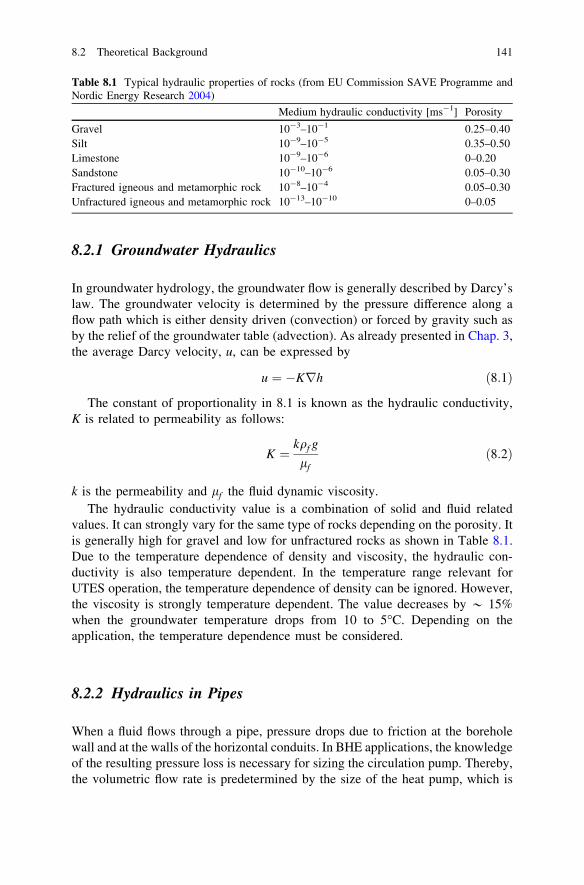
8.2.1 Groundwater Hydraulics

In groundwater hydrology, the groundwater flow is generally described by Darcy’slaw. The groundwater velocity is determined by the pressure difference along aflow path which is either density driven (convection) or forced by gravity such asby the relief of the groundwater table (advection). As already presented in Chap. 3,the average Darcy velocity, u, can be expressed by

u ¼ �Krh ð8:1Þ

The constant of proportionality in 8.1 is known as the hydraulic conductivity,K is related to permeability as follows:

K ¼kqf g

lfð8:2Þ

k is the permeability and lf the fluid dynamic viscosity.The hydraulic conductivity value is a combination of solid and fluid related

values. It can strongly vary for the same type of rocks depending on the porosity. Itis generally high for gravel and low for unfractured rocks as shown in Table 8.1.Due to the temperature dependence of density and viscosity, the hydraulic con-ductivity is also temperature dependent. In the temperature range relevant forUTES operation, the temperature dependence of density can be ignored. However,the viscosity is strongly temperature dependent. The value decreases by * 15%when the groundwater temperature drops from 10 to 5�C. Depending on theapplication, the temperature dependence must be considered.

8.2.2 Hydraulics in Pipes

When a fluid flows through a pipe, pressure drops due to friction at the boreholewall and at the walls of the horizontal conduits. In BHE applications, the knowledgeof the resulting pressure loss is necessary for sizing the circulation pump. Thereby,the volumetric flow rate is predetermined by the size of the heat pump, which is

Table 8.1 Typical hydraulic properties of rocks (from EU Commission SAVE Programme andNordic Energy Research 2004)

Medium hydraulic conductivity [ms-1] Porosity

Gravel 10-3–10-1 0.25–0.40Silt 10-9–10-5 0.35–0.50Limestone 10-9–10-6 0–0.20Sandstone 10-10–10-6 0.05–0.30Fractured igneous and metamorphic rock 10-8–10-4 0.05–0.30Unfractured igneous and metamorphic rock 10-13–10-10 0–0.05

8.2 Theoretical Background 141

http://dx.doi.org/10.1007/978-1-4471-4273-7_3

defined by the energy demand of the individual building. The volumetric flow rateitself defines then the flow velocity vpipe in the pipe. Considering 1D flow in thepipe, the pressure loss, Dp, along the BHE length, l, in a pipe of diameter, dpipe, isdefined by:

Dp ¼ fl

dpipe

qv2pipe

2þXn

i¼1

ni

qv2pipe

2ð8:3Þ

f is the borehole friction factor, n the friction factor of pipe fixtures (n ¼ 1 for thepipe turn point fixtures at the bottom; a list of n for various pipe fixtures can befound in the literature) and i is the number of pipe fixtures.

Depending on laminar or turbulent flow regimes different formulations of theborehole friction factor, f, are applicable. The flow regime in pipes is described bythe dimensionless Reynolds Number, Re:

Re ¼ vpipedpipe

mf¼

vpipedpipeqf

lfð8:4Þ

mf is the fluid kinematic viscosity and can be calculated from the fluid dynamicviscosity, lf , and the fluid density, qf . Generally,

• Re \ 2,300 laminar flow• 2,300 \ Re \ 104 transient between laminar and turbulent flow• Re [ 104 fully developed turbulent flow

In practice, flow regimes with Re [ 2,300 are often treated as turbulent.For laminar flow, f increases linearly with the flow velocity and is given by:

f ¼ 64Re¼ 64mf

vpipedpipe

ð8:5Þ

For turbulent flow, the Blasius approximation is often used and f is defined as:

f ¼ 0:3164

Re14

¼ 0:3164mf

vpipedpipe

� �14

ð8:6Þ

For both flow regimes, f is dependent on the viscosity of the heat carrier fluid.As well known, the viscosity is temperature dependent. The same applies forf here.

Much of the frictional pressure loss is due to the dependence of fluid flow on thepipe diameter of the pipe. Clearly, when reducing the pipe diameter by half, theflow velocity is squared for fixed flow rate. Due to the quadratic dependency ofpressure loss on flow velocity in Eq. 8.3, this will lead to a 4th order change inpressure loss. In installing less expensive, smaller pipes the pressure loss willincrease which requires stronger circulation pumps and thus, may lead to inefficientBHE systems.

142 8 Modeling

8.2.3 Heat Transfer

Heat is mainly transported by three mechanisms:

• Conduction

Conductive heat transfer occurs due to an energy transmission of molecularvibration. The heat is conducted through a medium in which there is a spatialvariation in temperature. Heat conduction is the dominant thermal process in solidrocks. The basic relation for conductive heat transport is Fourier’s law. It statesthat the conductive heat flow, qcon, at a point is proportional to the temperaturegradient, rT , at that point:

qcon ¼ �krT ð8:7Þ

k is the thermal conductivity.

• Advection

Advective heat transport is associated with the motion of a fluid. Although thethermal conductivity of water is low (0.6 W/m�K compared to an average value of2.5 W/m�K for sedimentary rocks), groundwater flow can transport a large amountof thermal energy by advection through pores and fractures due to its high heatcapacity. Therefore, advective heat transport can have a significant impact on BHEperformance. Groundwater movement is mainly due to differences in pressure. Thespecific thermal power qadv which is provided by advective mechanisms can becalculated as follows:

qadv ¼ qf Cf vfrT ð8:8Þ

Cf is specific fluid heat capacity.

• Heat transfer

If two bodies of different temperature are in contact, heat is transferred from thewarm body to the cold one. This mechanism is called heat transfer. The heat flow,qtrans, is proportional to the temperature difference of the two bodies:

qtrans ¼ h T1 � T2ð Þ ð8:9Þ

h is the heat transfer coefficient and Tis are the temperatures of the two bodies.

8.2.3.1 Heat Transport in the Ground

In principle, the subsurface can be treated as two different systems: a fluid and asolid phase. The fluid phase is defined as the groundwater in pores and fracturesand the solid phase represents the rock matrix. We get energy balance equation forthe fluid phase, f:


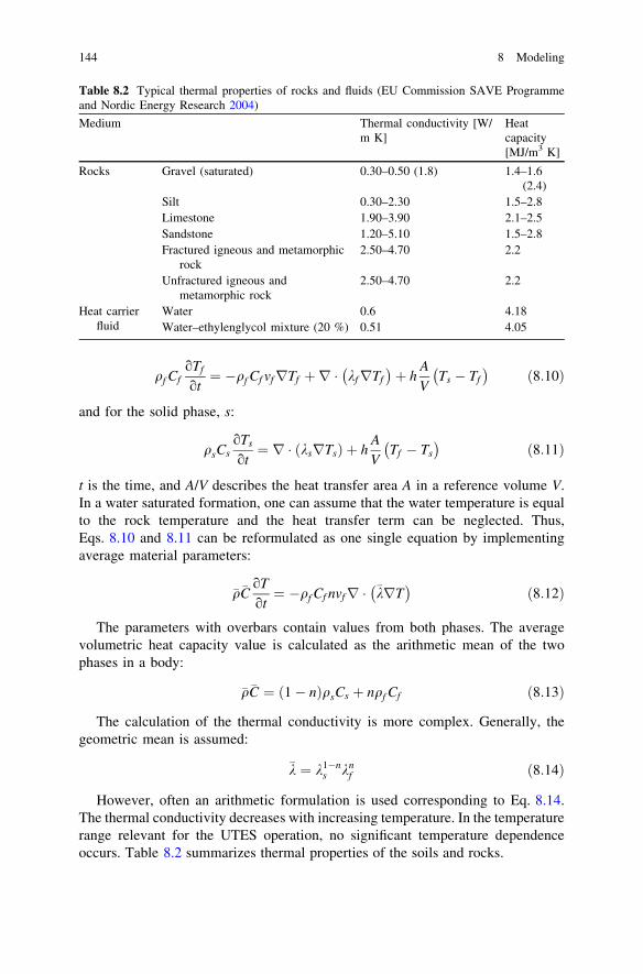
qf CfoTf

ot¼ �qf Cf vfrTf þr � kfrTf

� �þ h

A

VTs � Tf

� �ð8:10Þ

and for the solid phase, s:

qsCsoTs

ot¼ r � ksrTsð Þ þ h

A

VTf � Ts

� �ð8:11Þ

t is the time, and A/V describes the heat transfer area A in a reference volume V.In a water saturated formation, one can assume that the water temperature is equalto the rock temperature and the heat transfer term can be neglected. Thus,Eqs. 8.10 and 8.11 can be reformulated as one single equation by implementingaverage material parameters:

�q�CoT

ot¼ �qf Cf nvfr � �krT

� �ð8:12Þ

The parameters with overbars contain values from both phases. The averagevolumetric heat capacity value is calculated as the arithmetic mean of the twophases in a body:

�q�C ¼ 1� nð ÞqsCs þ nqf Cf ð8:13Þ

The calculation of the thermal conductivity is more complex. Generally, thegeometric mean is assumed:

�k ¼ k1�ns kn

f ð8:14Þ

However, often an arithmetic formulation is used corresponding to Eq. 8.14.The thermal conductivity decreases with increasing temperature. In the temperaturerange relevant for the UTES operation, no significant temperature dependenceoccurs. Table 8.2 summarizes thermal properties of the soils and rocks.

Table 8.2 Typical thermal properties of rocks and fluids (EU Commission SAVE Programmeand Nordic Energy Research 2004)

Medium Thermal conductivity [W/m K]

Heatcapacity[MJ/m3 K]

Rocks Gravel (saturated) 0.30–0.50 (1.8) 1.4–1.6(2.4)

Silt 0.30–2.30 1.5–2.8Limestone 1.90–3.90 2.1–2.5Sandstone 1.20–5.10 1.5–2.8Fractured igneous and metamorphic

rock2.50–4.70 2.2

Unfractured igneous andmetamorphic rock

2.50–4.70 2.2

Heat carrierfluid

Water 0.6 4.18Water–ethylenglycol mixture (20 %) 0.51 4.05

144 8 Modeling

The ratio between thermal conductivity and heat capacity can be described bythe thermal diffusivity, a:

a ¼�k

�q�Cð8:15Þ

The heat advection in porous media is only provided by the fluid phase. Sincethe advective part is weighted by porosity, the convective thermal front progresseswith the Darcy velocity. The ratio between the convective and the conductivetransport is given by the Peclet Number:

Pe ¼qf Cf vf L

�kð8:16Þ

L is the characteristic length (e.g. flow path).

8.2.3.2 Heat Transport in Pipes

Inside the pipe, the axial heat conduction is insignificant compared with theadvection of heat by the fluid due to the low thermal conductivity of the heatcarrier fluids. There is only 1D heat flow inside the pipe and heat transport can besimplified by:

qf CfoTf

otffi �qf Cf vfrTf ð8:17Þ

During operation, the heat from the BHE surroundings is transferred into thecirculation fluid by heat transport through the pipe wall. At the pipe wall, twoindependent thermal regimes are in contact, and the temperature for the fluid andsolid phase cannot be assumed as identical. Therefore, a heat transfer coefficientbetween the wall heat flux and the excess fluid becomes necessary. The heattransport through the pipe wall is defined as:

qpipeCpipe

oTpipe

ot¼ r � kpiperTpipe

� �þ h

A

VTf � Tpipe

� �ð8:18Þ

Only heat conduction in the radial direction has to be considered which can besimplified by a radial 1D process. If lateral temperature changes in the pipe fluidcan be neglected (i.e. perfect lateral heat transport inside the pipe), then the heattransfer is limited to the pipe wall. The heat transfer coefficient at the interface, h,is found from the 1D Fourier equation:

q ¼ h Tpipe � Tf

� �ð8:19Þ

The fluid mechanics literature commonly introduces a dimensionless measureof the heat transfer coefficient known as the Nusselt Number, Nu, the ratio of totalto conductive heat transport:


Nu ¼ hdpipe

kf¼

h Tpipe � Tf

� �

kf Tpipe�Tfð Þd

¼ qtotal

qcond

ð8:20Þ

Depending on laminar or turbulent flow regimes, different formulations of theNusselt Number are applicable. For laminar flow, the Nusselt Number can becalculated from the Prandtl Number, Pr, the Reynolds Number, Re, the dynamicviscosity of the fluid, lf , and the dynamic viscosity at the wall temperature, lw,formulated as the Sider–Tate equation:

Nu ¼ 1:86dpipeRe Pr

l

� �13 lf

lw

� �0:14

ð8:21Þ

l is the pipe length.In the temperature range relevant for BHE operation, the dynamic viscosity does

not vary strongly for the wall temperature and the fluid temperature. The last term inEq. 8.21 is close to 1 even for a temperature difference of 10 K. A different correlationmust be used for turbulent flow. An equation of the Dittus-Boelter form is often used:

Nu ¼ 0:023Re45 Pr

mð8:22Þ

The exponent of the Prandtl Number slightly varies depending on which cor-relation is used. For the Dittus-Boelter equation it is:

• m ¼ 0:4 if Tpipe [ Tfluid (Fluid is heated)• m ¼ 0:3 if Tpipe\Tfluid (Fluid is cooled)

The Prandtl Number is a material constant and defined as the ratio of thekinematic viscosity, m, and the thermal diffusivity, a:

Pr ¼ mf

a¼ mf

kf

qf Cf

¼qf lf

kfð8:23Þ

Basically, there are three approaches used to simulate BHEs. One is the ana-lytical method, like the line source model and the cylindrical model, another onebeing the response factor method, e.g., Eskilson’s model, Helltröm’s model, andYavuzturk’s model. The third one is the numerical method, for example Gu’smodel and Zeng’s model (He 2007).

8.3 Numerical Models

A large number of computer models dealing with UTES have been developedduring last decades. The suitability of models dealing with ATES and BTESapplications range from predesign to detailed design as summarized in Table 8.3(EU Commission SAVE Programme and Nordic Energy Research 2004).

146 8 Modeling

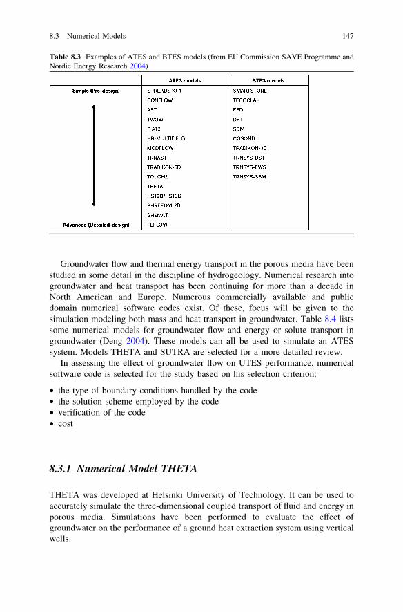
Groundwater flow and thermal energy transport in the porous media have beenstudied in some detail in the discipline of hydrogeology. Numerical research intogroundwater and heat transport has been continuing for more than a decade inNorth American and Europe. Numerous commercially available and publicdomain numerical software codes exist. Of these, focus will be given to thesimulation modeling both mass and heat transport in groundwater. Table 8.4 listssome numerical models for groundwater flow and energy or solute transport ingroundwater (Deng 2004). These models can all be used to simulate an ATESsystem. Models THETA and SUTRA are selected for a more detailed review.

In assessing the effect of groundwater flow on UTES performance, numericalsoftware code is selected for the study based on his selection criterion:

• the type of boundary conditions handled by the code• the solution scheme employed by the code• verification of the code• cost

8.3.1 Numerical Model THETA

THETA was developed at Helsinki University of Technology. It can be used toaccurately simulate the three-dimensional coupled transport of fluid and energy inporous media. Simulations have been performed to evaluate the effect ofgroundwater on the performance of a ground heat extraction system using verticalwells.

Table 8.3 Examples of ATES and BTES models (from EU Commission SAVE Programme andNordic Energy Research 2004)

8.3 Numerical Models 147

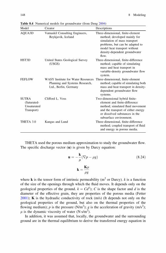
THETA used the porous medium approximation to study the groundwater flow.The specific discharge vector (u) is given by Darcy equation:

u ¼ � k

lrp� qgð Þ ð8:24Þ

k ¼ Klqg

where k is the tensor form of intrinsic permeability (m2 or Darcy). k is a functionof the size of the openings through which the fluid moves. It depends only on thegeological properties of the ground. k ¼ Cd2); C is the shape factor and d is thediameter of the effective grain, they are properties of the porous media (Fetter2001); K is the hydraulic conductivity of rock (m/s) (It depends not only on thegeological properties of the ground, but also on the thermal properties of theflowing medium); p is the pressure (N/m2); g is the acceleration of gravity (m/s2);l is the dynamic viscosity of water (N�s/m2).

In addition, it was assumed that, locally, the groundwater and the surroundingground are in the thermal equilibrium to derive the transferred energy equation in

Table 8.4 Numerical models for groundwater (from Deng 2004)

Model Creator Descriptions

AQUA3D Vatnaskil Consulting Engineers,Reykjavik, Iceland

Three-dimensional, finite-elementmethod; developed mainly forsimulation of mass transportproblems, but can be adapted tomodel heat transport withoutdensity-dependent groundwaterflow.

HST3D United States Geological Survey(USGS)

Three-dimensional, finite-differencemethod; capable of simulatingmass and heat transport invariable-density groundwater flowsystem.

FEFLOW WASY Institute for Water ResourcesPlanning and Systems Research,Ltd., Berlin, Germany

Three-dimensional, finite-elementmethod; capable of simulating bothmass and heat transport in density-dependent groundwater flowsystems.

SUTRA(Saturated-UnsaturatedTransport)

Clifford L. Voss Two-dimensional hybrid finite-element and finite-differencemethod; simulated fluid movementand the transport of either energyor dissolved substances in thesubsurface environment.

THETA 3.0 Kangas and Lund Three-dimensional, finite-differencemethod; coupled transport of fluidand energy in porous media.

148 8 Modeling

groundwater from the principle of conservation of energy. The resulting energyequation with an incompressible fluid is:

qCð ÞsoT

ot¼ r � krTð Þ � qCð Þf urT þ H ð8:25Þ

where qC is the volumetric heat capacity (J/m3�K); k is the thermal conductivity(W/m�K); u is the specific discharge (volume flow rate per unit of cross-sectionalarea) (m/s); H is the heat source or sink (W/m3); and subscripts: f is fluid (water);s is fluid saturated soil. The above two governing equations are discretized inTHETA using the explicit FDM and solved numerically.

The results from the THETA simulations suggest that an increase in groundwaterflow will result in improved system performance, which results from the energytransfer by groundwater; groundwater constantly replenishes the recoverable energyat the site of extraction. The presence of groundwater flow significantly increases theamount of recoverable energy. Similarly, standing column well systems, especiallywith groundwater bleed, make use of the energy stored in the aquifer.

The THETA aquifer simulation model has been incorporated into a computersimulation model AQSYST for simulating energy systems employing ATES.THETA simulates the thermo-hydraulic flow in the aquifer when either injectingwater to the well or extracting water from the well. It cannot model simultaneousinjection and extraction to/from a single well. The performance of standing col-umn well systems is characterized by circulating, injecting, and extracting water toand from an aquifer at the same time. Therefore, THETA cannot be applieddirectly to the standing column well system.

8.3.2 Numerical Model SUTRA

SUTRA (Saturated–Unsaturated Transport) is a computer program developed byVoss (1984). This numerical model simulates fluid movement and the transport ofeither energy or dissolved substances in the subsurface environment (aquifer).A two-dimensional hybrid finite-element and FDM is used to approximate thegoverning equations. SUTRA can solve the two interdependent processes:1. fluid density-dependent saturated or unsaturated groundwater flow and either2a. transport of a solute in the groundwater or2b. transport of thermal energy in the groundwater and solid matrix of the

aquifer

SUTRA was primarily intended to simulate two-dimensional flow, and eithersolute or energy transport in a saturated variable-density system. To simulate thegroundwater in unconfined aquifers affected by a periodic boundary condition,Ashtiani et al. (1999) modified the SUTRA model in three aspects:

8.3 Numerical Models 149

• the basic flow equation is changed from a pressure-based form to a mixed form• an automatic under-relaxation method is applied for adjustment of pressure after

each iteration to handle the nonlinearity of the unsaturated zone equations;• the model has been adjusted to handle a seepage-face boundary condition.

The validation tests of this two-dimensional numerical model for density-dependent groundwater flow in unconfined aquifers against experimental datawere successful.

Like THETA, SUTRA cannot model simultaneous heat/mass injection andextraction to/from a single well. So, SUTRA cannot be applied directly to thestanding column well system, either.

8.3.3 Other Numerical Models

A few other models address energy transfer in the aquifer. Hellström developed amodel that simulates the thermal process in the aquifer and in the surroundingground under certain simplifying assumptions concerning the groundwater flow(Breger et al. 1996). The basic assumption of the model is that the groundwaterflow is essentially radial in the thermally active region around the well. There areother assumptions that must be fulfilled:

• negligible regional groundwater flow;• negligible buoyancy flow caused by varying water temperature in the aquifer;• negligible influence of viscosity differences between different flow paths.

Convective heat transport and three-dimensional heat conduction are accountedfor in this model. The combined diffusive and convective heat flow processes inthe aquifer and the surrounding layers are solved using the explicit differencemethod (FDM).

Molson and Frind (1992) simulated the thermal energy storage in an unconfinedaquifer with a three-dimensional finite-element numerical model. In their model,the authors coupled the density-dependent groundwater flow and thermal energytransport. A symmetric matrix time integration scheme with the Galerkin FEM isemployed.

Chevalier and Banton (1999) applied the random walk method to model energytransfer in porous media. The method is based on the concept that cumulativeresults of repeated trials with an arbitrary probability distribution tend to aGaussian distribution. They compared their random results with the analyticalsolution and the numerical finite-difference solution. The results are similar in bothcases.

Because the above three models cannot model simultaneous heat/mass injectionand extraction to/from a single well, so they cannot be applied directly to thestanding column well system.

150 8 Modeling

References

Ashtiani BA, Volker RE, Lockington DA (1999) Numerical and experimental study of seepage inunconfined aquifers with a periodic boundary condition. J Hydrology 222(1–4):165–184

Breger DS, Hubbell JE, Hasnaoui HE, Sunderland JE (1996) Thermal energy storage in theground: comparative analysis of heat transfer modeling using U-tubes and boreholes. SolEnergy 56(6):493–503

Chevalier S, Banton O (1999) Modeling of heat transfer with random walk method, Part 1application to thermal energy storage in porous aquifers. J Hydrol 222(1–4):129–139

Deng Z (2004) Modeling of standing column wells in ground source heat pump systems, Ph.D.Dissertation, Oklahoma State University, Stillwater, OK, USA


Fetter CW (2001) Applied hydrogeology, 4th edn. Prentice Hall, Upper Saddle River, NJ, USAHe MM (2007) Analysis of underground thermal energy storage systems with ground water

advection in subtropical regions. Master’s Thesis, The University of Hong Kong, Hong KongMolson JM, Frind EO (1992) Thermal energy storage in an unconfined aquifer 2. model

development, validation, and application. Water Resour Res 28(10):2857–2867Ochs F, Heidemann W, Müller-Steinhagen H (2009) Modeling large-scale seasonal thermal

energy stores. In: Proceedings of Effstock 2009, Stockholm, Sweden, June 15–17Signorelli S (2004) Geoscientific investigations for the use of shallow low-enthalpy system. Sc.D.

dissertation, Swiss Federal Institute of Technology, Zurich, SwitzerlandVoss CI (1984) SUTRA: A finite element simulation model for saturated-unsaturated fluid-

density dependent ground-water flow with energy transport or chemically reactive singlespecies solute transport. US. Geological Survey, Reston, VA, USA

Yang H, Cui P, Fang Z (2010) Vertical-borehole ground-coupled heat pumps: a review of modelsand systems. Appl Energy 87(1):16–27

References 151

(green energy and technology) kun sang lee (auth.)-underground thermal energy...

Documents