Green Energy and Technology

Climate change, environmental impact and the limited natural resources urgescientific research and novel technical solutions. The monograph series GreenEnergy and Technology serves as a publishing platform for scientific andtechnological approaches to “green”—i.e. environmentally friendly and sustain-able—technologies. While a focus lies on energy and power supply, it also covers“green” solutions in industrial engineering and engineering design. Green Energyand Technology addresses researchers, advanced students, technical consultants aswell as decision makers in industries and politics. Hence, the level of presentationspans from instructional to highly technical.

More information about this series at http://www.springer.com/series/8059

Md. Rabiul Islam • Faz Rahman • Wei XuEditors

Advances in SolarPhotovoltaic Power Plants

123

EditorsMd. Rabiul IslamRajshahi University of Engineering andTechnology

RajshahiBangladesh

Faz RahmanUniversity of New South Wales (UNSW)Sydney, NSWAustralia

Wei XuHuazhong University of Scienceand Technology

Wuhan, HubeiChina

ISSN 1865-3529 ISSN 1865-3537 (electronic)Green Energy and TechnologyISBN 978-3-662-50519-9 ISBN 978-3-662-50521-2 (eBook)DOI 10.1007/978-3-662-50521-2

Library of Congress Control Number: 2016939060

© Springer-Verlag Berlin Heidelberg 2016This work is subject to copyright. All rights are reserved by the Publisher, whether the whole or partof the material is concerned, specifically the rights of translation, reprinting, reuse of illustrations,recitation, broadcasting, reproduction on microfilms or in any other physical way, and transmissionor information storage and retrieval, electronic adaptation, computer software, or by similar ordissimilar methodology now known or hereafter developed.The use of general descriptive names, registered names, trademarks, service marks, etc. in thispublication does not imply, even in the absence of a specific statement, that such names are exemptfrom the relevant protective laws and regulations and therefore free for general use.The publisher, the authors and the editors are safe to assume that the advice and information in thisbook are believed to be true and accurate at the date of publication. Neither the publisher nor theauthors or the editors give a warranty, express or implied, with respect to the material containedherein or for any errors or omissions that may have been made.

Printed on acid-free paper

This Springer imprint is published by Springer NatureThe registered company is Springer-Verlag GmbH Berlin Heidelberg

Contents

Introduction . . . . . . . . . . . . . . . . . . . . . . . . . . . . . . . . . . . . . . . . . . . . 1Md. Rabiul Islam

Photovoltaic Inverter Topologies for Grid Integration Applications . . . . 13Tan Kheng Suan Freddy and Nasrudin Abd Rahim

Advanced Control Techniques for PV Maximum Power PointTracking . . . . . . . . . . . . . . . . . . . . . . . . . . . . . . . . . . . . . . . . . . . . . . 43Wei Xu, Chaoxu Mu and Lei Tang

Maximum Power Point Tracking Methods for PV Systems . . . . . . . . . . 79Sarah Lyden, M. Enamul Haque and M. Apel Mahmud

Photovoltaic Multiple Peaks Power Tracking Using Particle SwarmOptimization with Artificial Neural Network Algorithm . . . . . . . . . . . . 107Mei Shan Ngan and Chee Wei Tan

Empirical-Based Approach for Prediction of Global Irradianceand Energy for Solar Photovoltaic Systems . . . . . . . . . . . . . . . . . . . . . 139Sivasankari Sundaram and J.S.C. Babu

A Study of Islanding Mode Control in Grid-Connected PhotovoltaicSystems . . . . . . . . . . . . . . . . . . . . . . . . . . . . . . . . . . . . . . . . . . . . . . . 169Wei Yee Teoh, Chee Wei Tan and Mei Shan Ngan

Stability Assessment of Power Systems Integrated with Large-ScaleSolar PV Units . . . . . . . . . . . . . . . . . . . . . . . . . . . . . . . . . . . . . . . . . . 215Naruttam Kumar Roy

Energy Storage Technologies for Solar Photovoltaic Systems . . . . . . . . 231Anjon Kumar Mondal and Guoxiu Wang

v

Superconducting Magnetic Energy Storage Modelingand Application Prospect . . . . . . . . . . . . . . . . . . . . . . . . . . . . . . . . . . 253Jian-Xun Jin and Xiao-Yuan Chen

Recycling of Solar Cell Materials at the End of Life . . . . . . . . . . . . . . . 287Teng-Yu Wang

vi Contents

About the Editors

Md. Rabiul Islam (M' 14, SM' 16, IEEE) receivedthe B.Sc. and M.Sc. degree from Rajshahi Universityof Engineering and Technology (RUET), Rajshahi,Bangladesh, in 2003 and 2009, respectively, both inelectrical and electronic engineering (EEE); and thePh.D. degree from University of Technology Sydney(UTS), Sydney, Australia, in 2014, in electricalengineering.

In 2005, he was appointed as a Lecturer in thedepartment of EEE, RUET where he was promoted asan Assistant Professor in 2008 and currently he is anAssociate Professor of the department. From 2013 to

2014, he was a Research Associate with the School of Electrical, Mechanical andMechatronic Systems, UTS. He has authored and coauthored more than 60 tech-nical papers, a book (Springer) and three book chapters (Springer and IET). Hisresearch interests are in the fields of power electronic converters, renewable energytechnologies, and smart grid.

Dr. Islam is a Senior member of the Institute of Electrical and ElectronicEngineers (IEEE), and member of Institution of Engineers, Bangladesh (IEB), andthe Australian Institute of Energy (AIE), Australia. He received the University GoldMedal and Joynal Memorial Award from RUET for his outstanding academicperformance while pursuing the B.Sc. engineering degree. He also received the BestPaper Awards at IEEE PECon-2012, ICEEE 2015, and ICCIE 2015. He acts as areviewer for several prestigious international journals.

vii

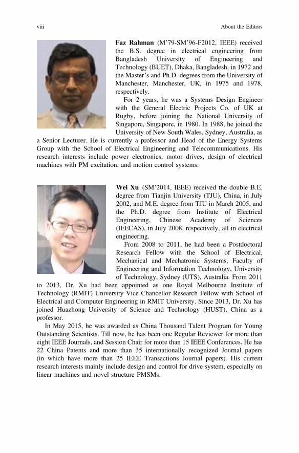
Faz Rahman (M’79-SM’96-F2012, IEEE) receivedthe B.S. degree in electrical engineering fromBangladesh University of Engineering andTechnology (BUET), Dhaka, Bangladesh, in 1972 andthe Master’s and Ph.D. degrees from the University ofManchester, Manchester, UK, in 1975 and 1978,respectively.

For 2 years, he was a Systems Design Engineerwith the General Electric Projects Co. of UK atRugby, before joining the National University ofSingapore, Singapore, in 1980. In 1988, he joined theUniversity of New South Wales, Sydney, Australia, as

a Senior Lecturer. He is currently a professor and Head of the Energy SystemsGroup with the School of Electrical Engineering and Telecommunications. Hisresearch interests include power electronics, motor drives, design of electricalmachines with PM excitation, and motion control systems.

Wei Xu (SM’2014, IEEE) received the double B.E.degree from Tianjin University (TJU), China, in July2002, and M.E. degree from TJU in March 2005, andthe Ph.D. degree from Institute of ElectricalEngineering, Chinese Academy of Sciences(IEECAS), in July 2008, respectively, all in electricalengineering.

From 2008 to 2011, he had been a PostdoctoralResearch Fellow with the School of Electrical,Mechanical and Mechatronic Systems, Faculty ofEngineering and Information Technology, Universityof Technology, Sydney (UTS), Australia. From 2011

to 2013, Dr. Xu had been appointed as one Royal Melbourne Institute ofTechnology (RMIT) University Vice Chancellor Research Fellow with School ofElectrical and Computer Engineering in RMIT University. Since 2013, Dr. Xu hasjoined Huazhong University of Science and Technology (HUST), China as aprofessor.

In May 2015, he was awarded as China Thousand Talent Program for YoungOutstanding Scientists. Till now, he has been one Regular Reviewer for more thaneight IEEE Journals, and Session Chair for more than 15 IEEE Conferences. He has22 China Patents and more than 35 internationally recognized Journal papers(in which have more than 25 IEEE Transactions Journal papers). His currentresearch interests mainly include design and control for drive system, especially onlinear machines and novel structure PMSMs.

viii About the Editors

Acronyms

µF Microfaradlm Micrometreµs Microsecond3L Three level3PI-P&O 3-point incremental perturb and observe7122-RC Model of inductorA AmpereABB ASEA Brown BoveriAC Alternating currentADC Analog to digital converterAESC Adaptive extremum seeking controlAFD Active frequency driftAFDPF Active frequency drift with positive feedbackAg SilverAl AluminiumANFIS Adaptive neuro-fuzzyANN Artificial neural networkARC Anti-reflection coatingAs2O3 Arsenic trioxidea-Si Amorphous silicona-Si/lc-Si Amorphous and micromorph silicon multi-junctionBDTk Bangladesh takaBST Bisection search theoremBST Binary signal transferBZO Boron-doped zinc oxideCAES Compressed air energy storageCCL Ceiling concentration limitCd CadmiumCdCO3 Cadmium carbonateCdS Cadmium sulfide

ix

CdSO4 Cadmium sulfateCdTe Cadmium telluridecf Chopping fractionCG Centralized generatorCGH2 Compressed gaseous hydrogenCI[G]S Copper–indium–[gallium]–[di]-sulphideCIGS Copper indium gallium selenidecm CentimetreCMV Common-mode voltageCO2 Carbon dioxideCPF Continuation power flowCPV Concentrator photovoltaicCSC Current source converterc-Si Crystalline siliconCVD Chemical vapor depositionCVS Controllable voltage sourceCVT Constant-voltage tracing methodDC Direct currentDC-AC Direct current to alternating currentDC-DC Direct current to direct currentDCI Double capacitor interfaceDFACTS Distributed FACTSDG Distributed generatorDGs Distributed generationDHESS Distributed HESSDHHS United States Department of Health and Human ServicesDL Distribution lineDLC Distribution line carrierDS1104 Model of dSPACE research & development controller boardDSMES Distributed SMESe− ElectronECA2DHG3R3 Model of capacitorEDLC Electrical double-layer capacitorEDLC Electrochemical double-layer capacitorEES Electrical energy storageEMI Electromagnetic interferenceENPH EnphaseEPA United States Environmental Protection AgencyEPIA European PV Industry AssociationESC Extremum seeking controlESS Energy storage systemEV Electric vehicleEVA Ethylene vinyl acetateFACTS Flexible AC transmission systemFC Fuel cell

x Acronyms

FCL Fault current limitingFCV FC vehicleFES Flywheel energy storageFLC Fuzzy logic controllerFRT Fault ride throughFulCurvE Full curve estimationG Solar irradianceg GramGa GalliumGa(NO3)3 Gallium nitrateGaInP Gallium indium phosphideGaN Gallium nitrideGe GermaniumGHG Green house gasGMPP Global maximum power pointGMPPT Global maximum power point trackingGP Global peakGPO Generalised perturb and observeGUI Graphical user interfaceGW GigawattGWP Gigawatt-peakH2 HydrogenH2O WaterH2SO4 Sulfuric acidHBZVR-D H-bridge zero voltage rectifier diodeHC Hill climbingHCPL3120 Model of gate drive optocouplerHCPSO Hybrid Chaotic PSOHERIC Highly efficient and reliable inverter conceptHESS Hybrid energy storage systemHEV Hybrid electric vehicleHF High frequencyHIT Heterojunction with intrinsic thin layerHNO3 Nitric acidHS300 33RJ Model of resistorHTS High temperature superconductingHVAC High-voltage alternating currentHVDC High-voltage direct currentHY5P Model of current transducerHz HertzIARC International Agency for Research on CancerIBC Interdigitated back contactIC Incremental conductanceIEC International Electrotechnical CommissionIEDs Intelligent Electronics Devices

Acronyms xi

IEEE Institute of Electrical and Electronics EngineersIGBT Insulated-gate bipolar transistorIn IndiumINC Incremental conductance methodIncCond Incremental conductanceInGaP Indium gallium phosphideIRF1640G Model of MOSFETI–V Current–VoltageK2TeO3 Potassium telluritekg KilogramkHz KilohertzKOH Potassium hydroxidekV KilovoltkW KilowattkWh Kilowatt hourLED Light-emitting diodeLF Low frequencyLH2 Liquid hydrogenLIB Lithium-ion batteryLP Local peakLV Low voltageLV25P Model of voltage transducerLVDC Low-voltage direct currentm2 Square meterMABE Mean absolute bias errorMAPE Mean absolute percentage errorMBE Mean bias errorMCL Maximum contaminant levelmg/kg Microgram per kilogrammg/L Microgram per litremH Milli HenryMLP Maximum loading pointmm MillimetreMMA MethylmethacrylateMo MolybdenumMOCVD Metal organic chemical vapor depositionMono-c-Si Monocrystalline siliconMOSFET Metal oxide semiconductor field effect transistorMPa MegapascalMPC Model predictive controlMPE Mean percentage errorMPP Maximum power pointMPPE Maximum power point estimationMPPT Maximum power point trackingMSE Mean squared error

xii Acronyms

MTOE Million tons of oil equivalentMulti-c-Si Multi crystalline siliconeMV Medium voltageMW MegawattMWp Megawatt-peakMWT Metal wrap throughNa2CO3 Sodium carbonateNa2SO4 Sodium sulfateNB Negative bigNDZ Non-detected ZoneNM Negative mediumNO2 Nitrogen dioxideNPC Neutral point clampedNS Negative smallOFP Over frequency protectionOP Operating pointOVP Over voltage protectionP&O Perturbation and observation methodPB Positive bigPCC Point of common couplingPCL Pollutant concentration limitPCS Power conditioning systemPCU Power conditioning unitP-D Power duty cyclePERC Passivated emitter rear cellsPET Polyethylene terephthalatePH Numeric scale used to specify the acidity or alkalinityPHEV Plug in electric vehiclePHS Pumped hydro storagePI Proportion integrationPID Proportional–integral–derivativePJD Phase jump detectionPLCC Power-line carrier communicationPM Positive mediumPMMA Poly-methyl-methacrylatePOI Potentially optimal intervalPOT Power operating triangleppmw Parts per million weightPS Positive smallPSAT Power system analysis toolboxPSCs Partially shaded conditionsPSO Particle swarm optimisationpu Per unitPV PhotovoltaicP–V Power–Voltage

Acronyms xiii

PVAS PV array simulatorPVF Polyvinyl fluoridePWM Pulse width modulationQ factor Quality factorR ReceiverRAM Random access memoryRCC Ripple correlation controlRCMU Residual current monitor unitRH Relative humidityRMSE Root-mean-square errorRTI Real-time interfaceS SulphurSA Simulated annealingSC Superconducting cableSCADA Supervisory control and data acquisitionSE Selective emitterSFS Sandia frequency shiftSHS Solar home systemSi SiliconSiC Silicon carbideSiNx Silicon nitrideSiOx Silicon oxideSISO Single input single outputSM Superconducting magnetSMC Sliding mode controlSMEE Superconducting magnetic energy exchangeSMES Superconducting magnetic energy storageSnO2 Tin oxideSO2 Sulfur dioxideSPD Signal produced by disconnectSSSC Static synchronous series compensatorSTATCOM Static synchronous compensatorSVS Sandia voltage shiftT TransmitterTCO Transparent conducting oxideTe TelluriumTe(SO4)2 Tellurium sulfateTeO2 Tellurium dioxideTF Thin filmTHD Total harmonic distortionTL Transmission lineTNB Tenaga nasional berhadTTZ Threshold tracking zoneU.S. United StatesU.S.EIA U.S. Energy Information Administration

xiv Acronyms

UFP Under frequency protectionUK United KingdomUL Underwriters LaboratoriesUPFC Unified power flow controllerUPS Uninterrupted power supplyUSA United States of AmericaUSD United state dollarUSD/kg United States dollar per kilogramUV UltravioletUVP Under voltage protectionV VoltVARC Capacitive loadVARL Inductive loadVFP Voltage protection and frequency protectionVSC Voltage source converterVWS Voltage window searchW WattW/m2 Waat per meter squaredWh Watt hourWS Wind speed (m/s)WSCC Western system coordinating councilwt% Percentage by weightZE ZeroZnS Zinc sulfide

Acronyms xv

Symbols

% PercentageoC Degree CelsiusVDC DC link voltage (V)VAN, VBN Phase voltages of converterP Positive terminal of the DC linkN Negative terminal of the DC linkA, B Terminals of single-phase systemCPV Stray capacitance (F)L1, L2 Filter inductors (H)IL Leakage current (A)RG Ground resistor (Ω)VCM Common-mode voltage (V)VDM Differential-mode voltage (V)VECM Equivalent common-mode voltage (V)Iph PV generated current (A)I0 PV cell reverse saturation current (A)q Electronic charge of an electron (1.6 � 10−19C)T Temperature of the PV cell (°C)S Solar radiation intensity (W/m2)K Boltzmann’s constant (1.38 � 10−23 J/K)A Constant factor (1.2 for Si-mono)i PV cell output current (A)u PV cell output voltage (V)Rs PV array series resistance (Ω)Rsh PV array shunt resistance (Ω)Isc Short-circuit current of PV array (A)Uoc Open-circuit voltage of PV array (V)Um MPP’s voltage for PV model (V)Im MPP’s current for PV model (A)P(u) Function of PV output power (W)

xvii

ISCref Current under standard conditions (A)UOCref Open-circuit voltage under standard conditions (V)Umref MPP’s voltage under standard conditions (V)Imref MPP’s current under standard conditions (A)Ropt Ratio of Umpp and Impp

DI0 Current error of inverter output (A)Iref Instantaneous current reference of inverter output (A)ig Instantaneous value of grid current (A)Uref Voltage reference of PV operating point (V)UPV Output voltage sample value of PV cells (V)C CapacitorD DiodeL Inductore Slope value of the continuous sampling points of attachmentDe Change in unit time slope on the PV cells P-U curveP(k) PV power for the k sampling times (W)I(k) PV current for the k sampling times (A)U(k) PV voltage for the k sampling times (V)dU Difference of voltage U(k)Pmpp Power of Maximum power point (W)Ui Corresponding voltage of language variable (V)i, j The subscriptsUdc Voltage of DC bus (V)Tp Time constant for neural network (s)Oi(k) Activation functionki(k) Input signal of neural networkWij Weight between neurons i and jN Total number of training samplest(k) Desired outputO(k) Actual outputM Total number of samples within a dayPMPP(k) Measured maximum power (W)IMPP(k) Corresponding current of PMPP(k) (A)UMPP(k) Corresponding voltage of PMPP(k) (V)Ep Total average error of maximum power within a dayEi Total average error of IMPP(k)Eu Total average error of UMPP(k)Pday Total maximum power (W)Iday Total optimal current (A)Uday Total average optimal voltage (V)P′(u) Slope of the PV P-U curveP″(u) Step change ratek Number of cyclea Scaling factorh Contingence angle

xviii Symbols

uL 0.02*UOC (V)uR 0.98*UOC (V)D(u) Step sizeNL(u) Scaling factorHL(u) Left tangent line through point (uL, P(uL)) of P-U curveHR(u) Right tangent line through point (uR, P(uR)) of P-U curved Value of thresholdLi Scaling factorX Input setsY Output setsf Distribution functionRpm Equivalent loadVmpp Voltage at MPP (V)Voc Open-circuit voltage (V)k1 Constant of proportionality for fractional open-circuit voltage

methodImpp Current at MPP (A)Isc Short-circuit current (A)k2 Constant of proportionality for fractional short-circuit current

methodΔI Change in current (A)M Scaling factordP Change in power (W)dV Change in voltage (V)dP0.5 Change in power due to MPP perturbation and environmental

change (W)dP1 Change in power due to irradiance change (W)P(k) Power at sample k (W)a1 Scaling factor for Generalised Perturb and Observeb Variable for Beta methodIpv Measured photovoltaic current (A)Vpv Measured photovoltaic voltage (V)c Constant for Beta methodq Electron charge (1.6 � 10−19 C)A Diode ideality factork Boltzmann constant (1.38 � 10−23 J/K)T Temperature (K)Ns Number of series connected cellsP1 Power sample for parabolic curve prediction (W)P2 Power sample for parabolic curve prediction (W)P3 Power sample for parabolic curve prediction (W)d1 Duty cycle sample for parabolic curve predictiond2 Duty cycle sample for parabolic curve predictiond3 Duty cycle sample for parabolic curve predictionxik Previous particle position (V)

Symbols xix

xik+1 New particle position (V)Uik+1 Particle new velocity

xi Inertia weightc1, c2 Acceleration coefficientsr1, r2 Random numbersPbest,i Power at best position of particle i (W)Gbest Power at global best position (W)Pk Power at candidate voltage (W)Pi Power at reference voltage (W)Tk Temperature of the search (°C)Pr Acceptance probabilityM Number of particlesvik Velocity vectorvik+1 New velocity vectorSik Current position

Sik+1 New position

pbesti Previous best positiongbest Global best positionw Initial weightc1 Cognitive coefficientc2 Social coefficientr1, r2 Random parameterIPV PV currentISC Short-circuit currentPPV Maximum PV powerIc Initial PV currentΔP Change of PV powerQ SwitchRload Resistive loadfs Switching frequencyIPSO PV current generated by PSOe Error signalkp Proportional constantki Integral constantkd Derivative constantVOC Open-circuit voltagePmax Maximum powerVDS Drain-source voltageVsensor Voltage sensing subsystemIsensor Current sensing subsystemIsensor_out Value subtracted by the current value from the current sensing

blockPPSO-ANN Power generated by PSO-ANNE Tracking efficiencyPmppt Power generated by MPPT

xx Symbols

EPSO-ANN Tracking efficiency for PSO-ANNEPSO Tracking efficiency for PSOH Monthly mean daily global horizontal irradiance (kWh/m2/day)H0 Monthly mean daily extraterrestrial irradiance (kWh/m2/day)a Empirical constant for the existing or the proposed empirical

modelb Empirical constant for the existing or the proposed empirical

modelS Monthly mean daily sunshine hour (h)S0 Maximum possible monthly average daily sunshine hour (h)c Empirical constant for the existing or the proposed empirical

modeld Empirical constant for the existing or the proposed empirical

modelTmax Maximum ambient temperature (oC)Tmin Minimum ambient temperature (oC)ΔT Temperature differenceP Precipitation data (mm)d Declination angle in degree (o)Tso Soil temperature (oC)Ta Monthly mean daily ambient temperature (oC)Pv Water vapour pressure (Pa)Tm Monthly mean daily module temperature (oC)L Latitude of the location (degree (o))Dn nth day of the yearh Hoursxs Hour angle (degree (o))R2 Regression coefficientZ Zenith angle (degree (o))a Solar altitude angle (degree (o))/ Longitude of a location (degree (o))e Empirical constant for the existing or the proposed empirical

modelf Empirical constant for the existing or the proposed empirical

modelTs Temperature of the sun (degree (o))N Number of training data setsEdc Monthly average daily DC energy generated (W)Eac Monthly average daily AC energy generated (W)ηpv Monthly average daily PV module efficiency (%)ηinv Monthly average daily inverter efficiency (%)U Overall heat transfer coefficient (W/m2 °C)A Area of the PV module or array (m2)hc Conductive heat transfer coefficient (W/m2 °C)ʋs Wind speed (m/s)

Symbols xxi

Exth Thermal exergy loss (W)Hz HertzIPV_inv Inverter’s output currentkm Kilometrekm2 Square kilometrekVA Kilovolt-ampskWh KiloWatt hourkWp KiloWatt peakmH MillihenryMtoe Tonne of oil equivalentMW MegaWattMWp MegaWatt-peakp piQf Quality factorTWh TeraWatt hourV VoltageVARC Reactive power consume by capacitive loadsVARL Reactive power consume by inductive loadsVPCC Inverter’s terminal voltageW WattWh/m2 Watt-hours per square metred1 Acceptable varianceDP Reactive power variationDQ Real power variationlF MicrofaradX Ohmt Times SecondR ResistanceX ReactanceB Susceptanced Rotor angleXb Base frequencyx Rotor speedPm Input mechanical powerPe Output electrical powerD Damping constantM Machine inertiae′d d-axis transient voltagee′q q-axis transient voltagefs System frequencyXd d-axis synchronous reactanceXq q-axis synchronous reactanceX′d d-axis transient reactanceX′q q-axis transient reactance

xxii Symbols

id d-axis stator currentiq q-axis stator currentEf Field voltageT′d0 d-axis rotor open-circuit time constantT′q0 q-axis rotor open-circuit time constantvd d-axis stator voltagevq q-axis stator voltagera Stator resistanceV Bus voltageh Bus anglePref Real power referenceQref Reactive power referenceVref Voltage referenceVpcc Voltage at the point of common couplingTp, Tq Converter time constantss Laplace operatorP Real powerQ Reactive poweridref d-axis reference current of PV converteriqref q-axis reference current of PV converterSi Nominal power of generator iHi Inertial constant of generator iHsys Average inertia constant of the systemV VoltageI CurrentL InductanceK KelvinE EnergyC CapacitanceU Output voltage from a controllable voltage source (V)Rline Power-line resistance (X)Rload Power-load resistance (X)UR(t) Transient voltage across the power-load resistor (V)Ur Rated voltage (V)Umin Minimum reference voltage (V)Umax Maximum reference voltage (V)IL(t) Transient current through the superconducting magnet (A)I(t) Transient current through the power-line resistor (A)IR(t) Transient current through the power-load resistor (A)IC(t) Transient current through the DC-link capacitor (A)U0 Initial voltage across the power-load resistor (V)I0 Initial current through the superconducting magnet (A)L Inductance of the superconducting magnet (H)C Capacitance of the DC-link capacitor (F)RSC Equivalent lossy resistance (X)

Symbols xxiii

Ic Critical current (A)ILr Rated current (A)Nlayer Number of the coil layerIdc Magnitude of the DC coil current (A)Im Magnitude of the AC coil current (A)f Frequency of the AC coil current (Hz)S(t) Current changing rate (A/s)Phys Hysteresis loss (W)Pflow Flux flow loss (W)Pcoup Coupling current loss (W)Peddy Eddy current loss (W)Pac AC loss (W)Qhys Energy consumption from hysteresis loss (J)Qflow Energy consumption from flux flow loss (J)Qcoup Energy consumption from coupling current loss (J)Qeddy Energy consumption from eddy current loss (J)B⊥ Perpendicular magnetic flux density (T)B// Parallel magnetic flux density (T)VDSmax Drain-source breakdown voltage (V)Ron Turn-on resistance (X)Resr Equivalent series resistance (X)Pswell Mean surplus power (W)Pshort Mean shortfall power (W)Tabs Power absorption time duration (s)Tcom Power compensation time duration (s)ηtotal Charge–discharge efficiencyIfault(t) Transient fault current through the superconducting cable (A)R(t) Transient resistance from the superconducting cable (X)Rm Maximum resistance from the superconducting cable (X)s1 Time constant of the quench period (ms)s2 Time constant of the recovery period (ms)N Number of the coil turnsrinner Inner radius of the coil unit (m)router Outer radius of the coil unit (m)h Height of the coil unit (m)Stape Tape usage of the coil unit (m)Usc Fault current-dependent increased voltage (V)IA, IB Load voltage-dependent decreased currents (A)Ubus DC bus voltage (V)Uload(t) Transient load voltage (V)n-Si N-type siliconp-Si P-type siliconn+ Extrinsic doped n-typen++ Heavy doped n-typep+ Extrinsic doped p-type

xxiv Symbols

List of Figures

Introduction

Figure 1 World population in billion with projections to 2050 . . . . . . . 2Figure 2 Global CO2 emissions from fossil fuel burning

and average global temperature . . . . . . . . . . . . . . . . . . . . . . 2Figure 3 World annual growth of energy use by source

(2008–2013) . . . . . . . . . . . . . . . . . . . . . . . . . . . . . . . . . . . 3Figure 4 World cumulative and annual solar photovoltaic

installations . . . . . . . . . . . . . . . . . . . . . . . . . . . . . . . . . . . . 4Figure 5 Layout of 10 MW solar PV power plant

in Ramagundam, India . . . . . . . . . . . . . . . . . . . . . . . . . . . . 6

Photovoltaic Inverter Topologies for Grid IntegrationApplications

Figure 1 Configuration of PV systems: a module inverter,b string inverter, c multi-string inverter, d centralinverter [8] . . . . . . . . . . . . . . . . . . . . . . . . . . . . . . . . . . . . 16

Figure 2 Three-phase two-level centralized inverter configuration . . . . . 16Figure 3 The parallel connection of two central inverter

to MV network via a single transformer . . . . . . . . . . . . . . . . 16Figure 4 Three-level central inverter: a NPC, b T-Type . . . . . . . . . . . . 17Figure 5 A photo of 2.3 MW micro-inverter solar project

at Ontario, Canada’s Vine Fresh Produce . . . . . . . . . . . . . . . 18Figure 6 Commercial Enecsys micro-inverter . . . . . . . . . . . . . . . . . . . 18Figure 7 Commercial Enphase micro-inverter . . . . . . . . . . . . . . . . . . . 19Figure 8 String inverters with galvanic isolation: a with LF

transformer, b with HF transformer . . . . . . . . . . . . . . . . . . . 20Figure 9 Two-level string inverters: a full-bridge, b HERIC,

c H5, d H6 . . . . . . . . . . . . . . . . . . . . . . . . . . . . . . . . . . . . 20Figure 10 Three-level string inverters: a NPC, b T-type. . . . . . . . . . . . . 21

xxv

Figure 11 Block diagram of a 1.2 MW PV plant with SMC11000TL multi-string inverters . . . . . . . . . . . . . . . . . . . . . . . 22

Figure 12 DC–DC converters for multi-string inverter:a HF transformer-based converter, b boost converter . . . . . . . 23

Figure 13 Resonant circuit for single-phase transformerlessPV inverter . . . . . . . . . . . . . . . . . . . . . . . . . . . . . . . . . . . . 24

Figure 14 Simplified resonant circuit for single-phasetransformerless topology . . . . . . . . . . . . . . . . . . . . . . . . . . . 24

Figure 15 Simplified resonant circuit for single-phasetransformerless topology . . . . . . . . . . . . . . . . . . . . . . . . . . . 24

Figure 16 The simplest resonant circuit for single-phasetransformerless topology . . . . . . . . . . . . . . . . . . . . . . . . . . . 25

Figure 17 Galvanic isolation topology via DC- or ACdecoupling method . . . . . . . . . . . . . . . . . . . . . . . . . . . . . . . 26

Figure 18 Operation of DC decoupling topology in conduction mode . . . 27Figure 19 Operation of DC-decoupling topology in freewheeling

mode . . . . . . . . . . . . . . . . . . . . . . . . . . . . . . . . . . . . . . . . 27Figure 20 CMV clamping topology. . . . . . . . . . . . . . . . . . . . . . . . . . . 28Figure 21 Operation of DC decoupling topology with CMV

clamping branch in conduction mode . . . . . . . . . . . . . . . . . . 28Figure 22 Operation of DC decoupling topology with CMV

clamping branch in freewheeling mode . . . . . . . . . . . . . . . . . 29Figure 23 Full-bridge topology . . . . . . . . . . . . . . . . . . . . . . . . . . . . . . 29Figure 24 Output voltage (top) and grid current (bottom)

for bipolar modulation . . . . . . . . . . . . . . . . . . . . . . . . . . . . 30Figure 25 CMV (top) and leakage current (bottom) for bipolar

modulation . . . . . . . . . . . . . . . . . . . . . . . . . . . . . . . . . . . . 30Figure 26 H5 topology . . . . . . . . . . . . . . . . . . . . . . . . . . . . . . . . . . . 31Figure 27 Output voltage (top) and grid current (bottom)

for H5 topology . . . . . . . . . . . . . . . . . . . . . . . . . . . . . . . . . 31Figure 28 CMV (top) and leakage current (bottom) for H5 topology . . . . 32Figure 29 HERIC topology . . . . . . . . . . . . . . . . . . . . . . . . . . . . . . . . 33Figure 30 Output voltage (top) and grid current (bottom)

for HERIC topology . . . . . . . . . . . . . . . . . . . . . . . . . . . . . . 33Figure 31 CMV (top) and leakage current (bottom)

for HERIC topology . . . . . . . . . . . . . . . . . . . . . . . . . . . . . . 34Figure 32 H6 topology . . . . . . . . . . . . . . . . . . . . . . . . . . . . . . . . . . . 34Figure 33 Output voltage (top) and grid current (bottom)

for H6 topology . . . . . . . . . . . . . . . . . . . . . . . . . . . . . . . . . 35Figure 34 CMV (top) and leakage current (bottom) for H6 topology . . . . 36Figure 35 oH5 topology . . . . . . . . . . . . . . . . . . . . . . . . . . . . . . . . . . 36Figure 36 Output voltage (top) and grid current (bottom)

for oH5 topology . . . . . . . . . . . . . . . . . . . . . . . . . . . . . . . . 37Figure 37 CMV (top) and leakage current (bottom) for oH5 topology . . . 37

xxvi List of Figures

Figure 38 HBZVR-D topology . . . . . . . . . . . . . . . . . . . . . . . . . . . . . . 38Figure 39 Output voltage (top) and grid current (bottom)

for HBZVR-D topology . . . . . . . . . . . . . . . . . . . . . . . . . . . 39Figure 40 CMV (top) and leakage current (bottom)

for HBZVR-D topology . . . . . . . . . . . . . . . . . . . . . . . . . . . 39Figure 41 Loss distribution of various topologies at 1 kW . . . . . . . . . . . 40

Advanced Control Techniques for PV Maximum PowerPoint Tracking

Figure 1 Equivalent circuit model of PV cell . . . . . . . . . . . . . . . . . . . 45Figure 2 The output characteristics of PV module

under different irradiance and temperature: a andc are the I–U curves, b and d are the P–U curves . . . . . . . . . 47

Figure 3 Schematic diagram of MPPT . . . . . . . . . . . . . . . . . . . . . . . . 48Figure 4 The MPPT control based on the DC/AC inverter . . . . . . . . . . 49Figure 5 The MPPT control based on the front DC/AC inverter . . . . . . 50Figure 6 Single-stage grid-connected structure . . . . . . . . . . . . . . . . . . 51Figure 7 The three-loop control structure for the single-stage

grid-connected inverter MPPT control. . . . . . . . . . . . . . . . . . 52Figure 8 The double-loop control structure for MPPT

control of the single-stage grid-connected inverter . . . . . . . . . 52Figure 9 The PV P–U characteristic curve . . . . . . . . . . . . . . . . . . . . . 54Figure 10 The membership functions. . . . . . . . . . . . . . . . . . . . . . . . . . 54Figure 11 The MPPT control system based on neural network . . . . . . . . 56Figure 12 The three-layer feedforward neural network . . . . . . . . . . . . . . 57Figure 13 Variation of the power and slope of power versus voltage . . . . 59Figure 14 The diagram of the speed factor NL . . . . . . . . . . . . . . . . . . . 61Figure 15 The experimental results: a P&O method, b new method . . . . 63Figure 16 The principle of the new algorithm. . . . . . . . . . . . . . . . . . . . 64Figure 17 The flowchart of the improved variable step algorithm . . . . . . 65Figure 18 The starting waveforms of the PV output voltages:

a improved method, b P&O method . . . . . . . . . . . . . . . . . . . 66Figure 19 The curves of P′(u) and angle � . . . . . . . . . . . . . . . . . . . . . . 67Figure 20 The procedure of linear prediction algorithm:

a linear prediction, b error correction, c algorithmflowchart. . . . . . . . . . . . . . . . . . . . . . . . . . . . . . . . . . . . . . 69

Figure 21 Tracking trajectory in mathematical theory . . . . . . . . . . . . . . 70Figure 22 The simulation of Newton iteration and proposed

methods: a newton iteration method, b the proposedmethod . . . . . . . . . . . . . . . . . . . . . . . . . . . . . . . . . . . . . . . 70

Figure 23 The simulation results of linear iteration methodand P&O method . . . . . . . . . . . . . . . . . . . . . . . . . . . . . . . . 71

Figure 24 Experiment comparisons among different methods:a P&O method, b proposed method . . . . . . . . . . . . . . . . . . . 72

List of Figures xxvii

Figure 25 The principle of constant voltage tracking method . . . . . . . . . 73Figure 26 Experimental results of tracking voltage, current,

and power of probability method under partially shadedconditions: a two-stage MPPT algorithms, b probability methodunder partial shade . . . . . . . . . . . . . . . . . . . . . . . . . . . . . . . 75

Maximum Power Point Tracking Methods for PV Systems

Figure 1 Characteristics for three modules under non-uniformenvironmental conditions. a I–V, b P–V . . . . . . . . . . . . . . . . 80

Figure 2 MPP Locus . . . . . . . . . . . . . . . . . . . . . . . . . . . . . . . . . . . . 83Figure 3 Flowchart of the P&O method . . . . . . . . . . . . . . . . . . . . . . . 84Figure 4 Flowchart of the IncCond method . . . . . . . . . . . . . . . . . . . . 85Figure 5 Sample parabolic curve prediction . . . . . . . . . . . . . . . . . . . . 90

Photovoltaic Multiple Peaks Power Tracking Using ParticleSwarm Optimization with Artificial Neural Network Algorithm

Figure 1 Two PV modules connected in series with onePV module partially shaded . . . . . . . . . . . . . . . . . . . . . . . . . 110

Figure 2 The P–V characteristic curves: a comparison of partiallyshaded (series-connected) PV modules with andwithout bypass diode . . . . . . . . . . . . . . . . . . . . . . . . . . . . . 111

Figure 3 The flowchart of the proposed hybrid PSO-ANNMPPT algorithm . . . . . . . . . . . . . . . . . . . . . . . . . . . . . . . . 114

Figure 4 The block diagram of the specification of ANNalgorithm in the simulation . . . . . . . . . . . . . . . . . . . . . . . . . 115

Figure 5 Graphs of mean squared error (MSE) against differentnumber of epochs for ANN algorithm. . . . . . . . . . . . . . . . . . 115

Figure 6 The simulation blocks of the PSO-ANN MPPTPV system made in MATLAB/Simulink . . . . . . . . . . . . . . . . 116

Figure 7 The PV array simulation block that consistsof six series-connected PV modules . . . . . . . . . . . . . . . . . . . 117

Figure 8 The input parameters for the series-connected PV modules . . . 118Figure 9 Different shaded patterns of the twelve

series-connected PV modules . . . . . . . . . . . . . . . . . . . . . . . . 119Figure 10 The overview of the experimental verification setup . . . . . . . . 121Figure 11 The integration of the proposed PSO-ANN algorithm

for experiment in RTI model in Simulink . . . . . . . . . . . . . . . 122Figure 12 Subsystem of the proposed PSO-ANN algorithm

block as in Subsystem2 . . . . . . . . . . . . . . . . . . . . . . . . . . . . 123Figure 13 The insertion of PV models under partial shaded

condition in PVAS1 control screen, the P–V curveshown in RAM 3 is read and written into the PVAS1. . . . . . . 124

xxviii List of Figures

Figure 14 a The online searching of global peak for PV stringunder partial shaded condition in PVAS1 GUI controlscreen b a zoomed in view of the characteristic curves . . . . . . 125

Figure 15 The P–V characteristics graph and the I–Vcharacteristics graph, which are simulated usingMATLAB/Simulink to resemble the hardwareexperimental result . . . . . . . . . . . . . . . . . . . . . . . . . . . . . . . 126

Figure 16 The P–V characteristic curves for six series-connectedPV array at a series of solar irradiance combinationas tabulated in Table 3 . . . . . . . . . . . . . . . . . . . . . . . . . . . . 127

Figure 17 The trace of operating point under the P–V characteristiccurves for large-scale PV array: a PV array with eightshaded PV modules in Cases 1 and 2, b PV array with sixshaded PV modules in Cases 3 and 4, c PV array with threeshaded PV modules in Cases 5 and 6 . . . . . . . . . . . . . . . . . . 128

Figure 18 The PV waveforms correspond to solar irradiancestep change of a case 1, b case 2, c case 3 andd case 4 as stated in Table 5 for the second simulation . . . . . . 129

Figure 19 The PV power waveforms correspond to solarirradiance variations in Table 4 for the third simulation.a PV array with eight shaded PV modules in Cases 1 and 2,b PV array with six shaded PV modules in Cases 3 and 4,c PV array with three shaded PV modules inCases 5 and 6 . . . . . . . . . . . . . . . . . . . . . . . . . . . . . . . . . . 131

Figure 20 The voltage, current, and power waveforms of PVsystem for the first experiment, which is capturedin the LeCroy Oscilloscope . . . . . . . . . . . . . . . . . . . . . . . . . 133

Figure 21 The voltage, current, and power waveforms of PVsystem for the first experiment, which is simulatedin MATLAB/Simulink . . . . . . . . . . . . . . . . . . . . . . . . . . . . 134

Empirical-Based Approach for Prediction of Global Irradianceand Energy for Solar Photovoltaic Systems

Figure 1 Classification of empirical irradiance and energyprediction models . . . . . . . . . . . . . . . . . . . . . . . . . . . . . . . . 141

Figure 2 Methodology for empirical model formulation . . . . . . . . . . . . 146Figure 3 Variation of clearness index with respect to relative

sunshine hour as reported in [54] . . . . . . . . . . . . . . . . . . . . . 148Figure 4 a–c Significance of considered input factor sunshine

hour, temperature ratio and air mass towardsclearness index (response) . . . . . . . . . . . . . . . . . . . . . . . . . . 150

Figure 5 Monthly average daily variation of AC energy generationand global irradiance for 5 MWp PV . . . . . . . . . . . . . . . . . . 159

List of Figures xxix

Figure 6 Monthly average daily variation of final yieldfor 5 MWp PV plant. . . . . . . . . . . . . . . . . . . . . . . . . . . . . . 159

Figure 7 Monthly average thermal exergy loss generatedby 5 MWp PV system and the monitored temperaturedifference . . . . . . . . . . . . . . . . . . . . . . . . . . . . . . . . . . . . . 162

Figure 8 Variation of thermal exergy loss over AC energygenerated for a 5 MWp PV system . . . . . . . . . . . . . . . . . . . . 162

Figure 9 Variation of thermal exergy loss over AC energygenerated for a 160 kWp PV system . . . . . . . . . . . . . . . . . . . 162

Figure 10 Tm versus Eac for 67.84 kWp PV system [77] . . . . . . . . . . . . 163Figure 11 Comparison of MPE for the existing with the proposed

model for 5 MWp PV plant at Sivagangai during training(2011–2012) . . . . . . . . . . . . . . . . . . . . . . . . . . . . . . . . . . . 164

Figure 12 MPE of the energy prediction modelsfor a 1.72 kWp PV plant at Durban . . . . . . . . . . . . . . . . . . . 165

A Study of Islanding Mode Control in Grid-ConnectedPhotovoltaic Systems

Figure 1 The overview block diagram of Microgridsconnected to utility grid . . . . . . . . . . . . . . . . . . . . . . . . . . . 170

Figure 2 The grid-connected PV system at the PCCwhere anti-islanding control is present . . . . . . . . . . . . . . . . . 172

Figure 3 The classification of anti-islanding detection techniques . . . . . 175Figure 4 Local measuring parameters of local anti-islanding

detection method . . . . . . . . . . . . . . . . . . . . . . . . . . . . . . . . 176Figure 5 The passive islanding detection methods . . . . . . . . . . . . . . . . 177Figure 6 The flowchart of the passive islanding detection method . . . . . 177Figure 7 The power flow in a PV grid-connected system under

a normal operating condition . . . . . . . . . . . . . . . . . . . . . . . . 178Figure 8 The operation of voltage phase jump detection. . . . . . . . . . . . 180Figure 9 The active islanding detection methods . . . . . . . . . . . . . . . . . 184Figure 10 The flowchart of the active islanding detection method . . . . . . 185Figure 11 The path of the disturbance signals during an islanding

condition, a before the circuit breaker is openedand b after the circuit breaker is opened . . . . . . . . . . . . . . . . 186

Figure 12 Frequency bias islanding detection method: distortedcurrent waveform . . . . . . . . . . . . . . . . . . . . . . . . . . . . . . . . 187

Figure 13 The SFS islanding detection method: current waveformwith dead time and truncation . . . . . . . . . . . . . . . . . . . . . . . 188

Figure 14 The flowchart of the hybrid islanding detection method . . . . . 190Figure 15 Classification of remote islanding detection method . . . . . . . . 191Figure 16 Topology of Impedance Insertion Method, where a low

value impedance load had been added to the utility . . . . . . . . 192

xxx List of Figures

Figure 17 The illustration of Transfer Trip Scheme in a distributionsystem [23] . . . . . . . . . . . . . . . . . . . . . . . . . . . . . . . . . . . . 193

Figure 18 Topology of power line carrier communication controlwith transmitter (T) and receiver (R) added to the system . . . . 194

Figure 19 The VFP simulation model in MATLAB/Simulink . . . . . . . . . 200Figure 20 The RMS voltage when the frequency of the instantaneous

voltage input is increasing from 50 to 52 Hz at t = 0.2 s:a before filter or before the Average and low pass filterblock; b after the Average blocks; c after filteror the Average and low pass filter block; d comparisonsof (a–c). . . . . . . . . . . . . . . . . . . . . . . . . . . . . . . . . . . . . . . 201

Figure 21 The detection signals for VFP under the normal operation,Vpcc = 196 V and Fpcc = 49 Hz: a OFP/UFP checker, V = 0;b OVP/UVP checker, V = 0; c VFP controller, V = 1;d circuit breaker maintains at closed status . . . . . . . . . . . . . . 202

Figure 22 The detection signals for VFP under the UFP operation,Vpcc = 196 V and Fpcc = 48 Hz: a OFP/UFP checkertrigger UFP at t = 0.3504 s, V = 1; b OVP/UVP checker,V = 0; c VFP Controller detects islanding at t = 0.3506 s,V = 0; d circuit breaker opens at t = 0.3506 s . . . . . . . . . . . . 203

Figure 23 The detection signals for VFP under the OFP operation,Vpcc = 196 V and Fpcc = 52 Hz: a OFP/UFP checkertrigger OFP at t = 0.3602 s, V = 1; b OVP/UVP checker,V = 0; c VFP Controller detects islanding at t = 0.3602 s,V = 0; d circuit breaker opens at t = 0.3602 s . . . . . . . . . . . . 204

Figure 24 The AFD simulation model in Simulink . . . . . . . . . . . . . . . . 205Figure 25 The AFD signal generated from the AFD Controller. . . . . . . . 205Figure 26 The simulation output of AFD for Fpcc = 49.4 Hz,

cf = 0.049: a islanding detection time, t = 0.1006 s;b the load Vpcc stop at t = 0.1475 s; c islanding detected . . . . 206

Figure 27 The simulation output of AFD for Fpcc = 50.0 Hz,cf = 0.05: a islanding detection time, t = 0.1992 s;b the load Vpcc stop at t = 0.2253 s; c islanding detected . . . . 207

Figure 28 The simulation output of AFD for Fpcc = 50.4 Hz,cf = 0.0504: a islanding detection time, t = 0.1008 s;b the load Vpcc stop at t = 0.1455 s; c islanding detected . . . . 208

Figure 29 Comparison of detection time with various frequencyfor case, Qf = 1.0: Fpcc = 49.4 Hz (blue line); AFDislanding detection at t = 0.1006 s. Fpcc = 50.0 Hz(red dotted line); AFD islanding detection at t = 0.1992 s.Fpcc = 5.04 Hz (green dotted line); AFD islandingdetection at t = 0.1008 s . . . . . . . . . . . . . . . . . . . . . . . . . . . 209

List of Figures xxxi

Figure 30 Comparison of run on time with different Qf for the caseFpcc = 50.4 Hz, cf = 0.0504: Qf = 1.0 (blue line),the voltage transient stop at t = 0.1455 s; Qf = 2.5(red dotted line), the voltage transient stop at t = 0.1902 s(Color figure online). . . . . . . . . . . . . . . . . . . . . . . . . . . . . . 209

Stability Assessment of Power Systems Integratedwith Large-Scale Solar PV Units

Figure 1 WSCC 9-bus test system. . . . . . . . . . . . . . . . . . . . . . . . . . . 217Figure 2 Constant P, constant Q model . . . . . . . . . . . . . . . . . . . . . . . 219Figure 3 Constant P, constant V model . . . . . . . . . . . . . . . . . . . . . . . 219Figure 4 Constant P, constant Q model with converter. . . . . . . . . . . . . 219Figure 5 Constant P, constant V model with converter . . . . . . . . . . . . . 220Figure 6 Bus voltage of the system in different modes. . . . . . . . . . . . . 221Figure 7 Power imported from the grid . . . . . . . . . . . . . . . . . . . . . . . 221Figure 8 GUI for continuation power flow settings in PSAT. . . . . . . . . 222Figure 9 P–V curve under base case . . . . . . . . . . . . . . . . . . . . . . . . . 223Figure 10 Bus voltages of the system (PQ mode) . . . . . . . . . . . . . . . . . 224Figure 11 Speed deviation of synchronous generator

connected at bus 2 . . . . . . . . . . . . . . . . . . . . . . . . . . . . . . . 224Figure 12 Power output of synchronous generator connected

at bus 2 . . . . . . . . . . . . . . . . . . . . . . . . . . . . . . . . . . . . . . 224Figure 13 System frequency measured at bus 1, 2, and 3 . . . . . . . . . . . . 225Figure 14 Eigenvalues of the solar PV integrated system . . . . . . . . . . . . 225Figure 15 Loading parameter versus voltage curve under contingency . . . 226Figure 16 Voltage at bus 3. . . . . . . . . . . . . . . . . . . . . . . . . . . . . . . . . 226Figure 17 System frequency measured at bus 1, 2, and 3 . . . . . . . . . . . . 227Figure 18 Voltage at bus 2. . . . . . . . . . . . . . . . . . . . . . . . . . . . . . . . . 227Figure 19 Speed deviation of synchronous generator 1 . . . . . . . . . . . . . 228

Energy Storage Technologies for Solar Photovoltaic Systems

Figure 1 Illustration of the six forms of energy and relatedexamples of their inter-conversions [9] . . . . . . . . . . . . . . . . . 233

Figure 2 Schematic of applications of electricity storagefor generation, transmission, distribution, and endcustomers and future smart grid that integrateswith intermittent renewables and plug-in hybrid vehiclesthrough two-way digital communications betweenloads and generation or distribution grids [10] . . . . . . . . . . . . 235

Figure 3 Photovoltaic systems interconnected to the grid:a without energy storage, b utilizing energy storagewith the different options 1 local load management,2 load management for the utility, and 3 consideringcritical emergency loads [11] . . . . . . . . . . . . . . . . . . . . . . . . 236

xxxii List of Figures

Figure 4 Illustration of pumped hydro storage with the pumpingenergy supplied by PV array [17]. . . . . . . . . . . . . . . . . . . . . 238

Figure 5 Schematic diagram of compressed air energy storage [18] . . . . 239Figure 6 Supermagnetic energy storage system [20]. . . . . . . . . . . . . . . 240Figure 7 The working principle of supercapacitors. a Electric

double layer, b redox reaction on the surface and c redoxreaction in bulk [24] . . . . . . . . . . . . . . . . . . . . . . . . . . . . . . 242

Figure 8 Rechargeable cell/battery diagram [28] . . . . . . . . . . . . . . . . . 243Figure 9 NaS battery [28] . . . . . . . . . . . . . . . . . . . . . . . . . . . . . . . . 246Figure 10 Schematic of a LIB [36] . . . . . . . . . . . . . . . . . . . . . . . . . . . 248

Superconducting Magnetic Energy Storage Modelingand Application Prospect

Figure 1 Classification of energy storage systems . . . . . . . . . . . . . . . . 254Figure 2 Topology of a typical VSC based PCS . . . . . . . . . . . . . . . . . 257Figure 3 Topologies of three basic FACTS and DFACTS schemes . . . . 257Figure 4 Energy exchange circuit with a brige-type chopper . . . . . . . . . 258Figure 5 Digital state diagrams of the two I-V choppers:

a Bridge-type chopper; b Conventional chopper . . . . . . . . . . . 258Figure 6 2D axisymmetric model of the 0.2 H Bi-2223 solenoid coil. . . 260Figure 7 Magnetic field distributions of the 0.2 H Bi-2223 solenoid

coil when I(t) is 60 A: a parallel magnetic field;b perpendicular magnetic field . . . . . . . . . . . . . . . . . . . . . . . 260

Figure 8 Critical current and flux flow loss distributions of the fiveupper coil layers: a critical current distributionswhen IL(t) = 40 A; b critical current distributionswhen IL(t) = 60 A; c flux flow loss distributionswhen IL(t) = 40 A; d flux flow loss distributionswhen IL(t) = 60 A . . . . . . . . . . . . . . . . . . . . . . . . . . . . . . . 261

Figure 9 Perpendicular and parallel hysteresis loss distributions:a Phys⊥, Nlayer = 1 to Nlayer = 5, Im = Idc = 15 A, f = 10 Hz;b Phys⊥, Nlayer = 1 to Nlayer = 5, Im = Idc = 20 A, f = 10 Hz;c Phys//, Nlayer = 30 to Nlayer = 34, Im = Idc = 15 A, f = 10 Hz;d Phys//, Nlayer = 30 to Nlayer = 34, Im = Idc = 20 A,f = 10 Hz . . . . . . . . . . . . . . . . . . . . . . . . . . . . . . . . . . . . . 262

Figure 10 Perpendicular and parallel coupling current loss distributions:a Pcoup⊥, Nlayer = 1 to Nlayer = 5, S(t) = 50 A/s; b Pcoup⊥,Nlayer = 1 to Nlayer = 5, S(t) = 60 A/s; c Pcoup//, Nlayer = 30to Nlayer = 34, S(t) = 50 A/s; d Pcoup//, Nlayer = 30to Nlayer = 34, S(t) = 60 A/s . . . . . . . . . . . . . . . . . . . . . . . . 262

Figure 11 Calculated and fitted AC loss of the whole coil:a hysteresis loss; b flux flow loss; c coupling currentloss and eddy current loss . . . . . . . . . . . . . . . . . . . . . . . . . . 263

Figure 12 Principle of circuit-field-superconductor coupled method . . . . . 264

List of Figures xxxiii

Figure 13 Scheme of the SMEE model . . . . . . . . . . . . . . . . . . . . . . . . 265Figure 14 Simulated load voltage and coil current:

a UR(t) versus t b IL(t) versus t . . . . . . . . . . . . . . . . . . . . . . 266Figure 15 Simulated flux flow loss and energy consumption:

a Pflow(t) versus t b Qflow(t) versus t. . . . . . . . . . . . . . . . . . . 267Figure 16 Developed SMES prototype: a schematic diagram

b experiment setup . . . . . . . . . . . . . . . . . . . . . . . . . . . . . . . 269Figure 17 Measured results of UR(t) and IL(t) during a 100 W

energy exchange cycle: a UR(t) versus t b IL(t) versus t . . . . . 270Figure 18 Measured and calculated results of ηtotal during a 100 W

energy exchange cycle: a ηtotal versus I0b ηtotal versus Pref. . . . . . . . . . . . . . . . . . . . . . . . . . . . . . . . 271

Figure 19 Measured and calculated results during five 100 Wenergy exchange cycle: a UR(t) versus tb IL(t) versus t c Pmag(t) versus t d Qmag(t) versus t . . . . . . . . 272

Figure 20 Sketch of the LVDC micro photovoltaic grid . . . . . . . . . . . . . 274Figure 21 Simulation model of the LVDC micro photovoltaic grid . . . . . 275Figure 22 FCL SC circuit model. . . . . . . . . . . . . . . . . . . . . . . . . . . . . 275Figure 23 SMES circuit model . . . . . . . . . . . . . . . . . . . . . . . . . . . . . . 276Figure 24 Critical current (kA) distributions of a rectangular-shaped

coil and b step-shaped coil . . . . . . . . . . . . . . . . . . . . . . . . . 277Figure 25 Load voltage Uload(t) during a power sag period . . . . . . . . . . 278Figure 26 Coil current IL(t) during a power swell period and a voltage

sag period . . . . . . . . . . . . . . . . . . . . . . . . . . . . . . . . . . . . . 279Figure 27 Load voltage Uload(t) during a power swell period . . . . . . . . . 279Figure 28 Basic cooperative operation principle of the FCL SC

and SMES. . . . . . . . . . . . . . . . . . . . . . . . . . . . . . . . . . . . . 280Figure 29 Simulated results during a grounding fault: a Uload(t)

versus t b R(t) versus t (c) IA(t) versus t . . . . . . . . . . . . . . . . 281Figure 30 Simulated results with the cooperative operations of FCL

SC branch 5, SMES A and SMES B: a Uload1(t), Uload2(t)versus t b IA(t), IB(t) versus t. . . . . . . . . . . . . . . . . . . . . . . . 282

Recycling of Solar Cell Materials at the End of Life

Figure 1 Solar PV global annual installations and projected waste . . . . . 288Figure 2 Solar PV global cumulative installations

and projected waste . . . . . . . . . . . . . . . . . . . . . . . . . . . . . . 288Figure 3 Degradation of PV modules: a corrosion, b discoloration,

c delamination, d breakage and cracking [5–8]. . . . . . . . . . . . 289Figure 4 PV module performance degradation pathways [4] . . . . . . . . . 291Figure 5 Classification of solar cells . . . . . . . . . . . . . . . . . . . . . . . . . 292Figure 6 Structure of silicon solar cells: a commercial solar cell,

b SE solar cell, c MWT solar cell, d IBC solar cell,e bifacial solar cell, f PERC solar cell. . . . . . . . . . . . . . . . . . 293

xxxiv List of Figures

Figure 7 Structure of commercial silicon PV modules . . . . . . . . . . . . . 293Figure 8 Structure of PV modules with different solar cell types:

a rear-contact solar cells, b bifacial solar cells . . . . . . . . . . . . 294Figure 9 Structure of a silicon thin-film PV module . . . . . . . . . . . . . . 294Figure 10 Structure of the CdTe PV module . . . . . . . . . . . . . . . . . . . . 296Figure 11 a Structure of a GaAs solar cell, b structure

of a concentrator PV module . . . . . . . . . . . . . . . . . . . . . . . . 298Figure 12 Structure of a CIGS PV module . . . . . . . . . . . . . . . . . . . . . . 299Figure 13 Dissolution of EVA by organic solvent [19] . . . . . . . . . . . . . 302Figure 14 Residual components of silicon module

after heat decomposition . . . . . . . . . . . . . . . . . . . . . . . . . . . 302Figure 15 The recycling process for crystalline silicon PV modules. . . . . 303Figure 16 The recycling process for silicon thin-film PV modules. . . . . . 304Figure 17 The recycling process for CdTe PV modules . . . . . . . . . . . . . 305Figure 18 The CdTe PV module recycling process of First

Solar Inc. [27] . . . . . . . . . . . . . . . . . . . . . . . . . . . . . . . . . . 306Figure 19 The concentrator PV module assembly drawing . . . . . . . . . . . 307Figure 20 The recycling process for concentrator PV modules . . . . . . . . 307Figure 21 The recycling process for CIGS PV modules . . . . . . . . . . . . . 308Figure 22 The price and global production of gallium . . . . . . . . . . . . . . 310Figure 23 The price and global production of indium . . . . . . . . . . . . . . 311Figure 24 The price and global production of silver . . . . . . . . . . . . . . . 312Figure 25 The price and global production of germanium . . . . . . . . . . . 312

List of Figures xxxv

List of Tables

Introduction

Table 1 Performance of commercial solar PV technologies. . . . . . . . . . 5

Advanced Control Techniques for PV Maximum PowerPoint Tracking

Table 1 Rules of fuzzy controller . . . . . . . . . . . . . . . . . . . . . . . . . . . 55

Photovoltaic Multiple Peaks Power Tracking Using ParticleSwarm Optimization with Artificial Neural Network Algorithm

Table 1 Two samples of Ic and �P; trained in ANN algorithm. . . . . . . 113Table 2 The specifications of 8U-50P polycrystalline solar module . . . . 118Table 3 Combinations of solar irradiance level with the corresponding

maximum power for six series-connected PV modules(small-scale) . . . . . . . . . . . . . . . . . . . . . . . . . . . . . . . . . . . . 119

Table 4 Combinations of solar irradiance level with the correspondingmaximum power for twelve series-connected PVmodules (large-scale) . . . . . . . . . . . . . . . . . . . . . . . . . . . . . . 120

Table 5 Combinations of solar irradiance step change . . . . . . . . . . . . . 121Table 6 The specification of electronic components used

for hardware setup. . . . . . . . . . . . . . . . . . . . . . . . . . . . . . . . 122Table 7 The specifications of PV string in PVAS1 . . . . . . . . . . . . . . . 126Table 8 The comparison of the maximum PV power

and the generated tracked power for the small-scalePV array . . . . . . . . . . . . . . . . . . . . . . . . . . . . . . . . . . . . . . 129

Table 9 The comparisons of maximum PV powerand the generated MPPT power of the large-scalePV array . . . . . . . . . . . . . . . . . . . . . . . . . . . . . . . . . . . . . . 132

Table 10 The comparison of the experimental resultand its compatible simulation result . . . . . . . . . . . . . . . . . . . . 135

xxxvii

Empirical-Based Approach for Prediction of GlobalIrradiance and Energy for Solar Photovoltaic Systems

Table 1 Training data set of proposed model parameters(comprising the measured and evaluated inputparameters) for Madurai/Sivagangai during (1961–1990) . . . . . 152

Table 2 Empirical constants for the proposed modelfor Madurai/Sivagangai . . . . . . . . . . . . . . . . . . . . . . . . . . . . 152

Table 3 Training data set of proposed model parameters(comprising the measured and evaluated inputparameters) for Chennai during (1961–1990) . . . . . . . . . . . . . 153

Table 4 Empirical constants for the proposed model for Chennai . . . . . 153Table 5 Sunshine-based empirical constants

for Madurai/Sivagangai . . . . . . . . . . . . . . . . . . . . . . . . . . . . 155Table 6 Sunshine based empirical constants for Chennai . . . . . . . . . . . 156Table 7 Performance comparison for the proposed models

during validation for Sivagangai . . . . . . . . . . . . . . . . . . . . . . 156Table 8 Performance comparison among the existing

and the reported multi-parametric models for Sivagangai . . . . . 156Table 9 Performance comparison among the existing

and the reported models for Chennai during validation. . . . . . . 157Table 10 Effect of variation of H and Ta towards energy

generation and efficiency . . . . . . . . . . . . . . . . . . . . . . . . . . . 160

A Study of Islanding Mode Control in Grid-ConnectedPhotovoltaic Systems

Table 1 Comparison of islanding detection method basedon various characteristics . . . . . . . . . . . . . . . . . . . . . . . . . . . 196

Table 2 Voltage and frequency limits for VFP under standard MS;IEC 61727 and 62116 . . . . . . . . . . . . . . . . . . . . . . . . . . . . . 199

Table 3 VFP method simulation parameters . . . . . . . . . . . . . . . . . . . . 200

Stability Assessment of Power Systems Integratedwith Large-Scale Solar PV Units

Table 1 Data of WSCC 9-bus system . . . . . . . . . . . . . . . . . . . . . . . . 218Table 2 MLP of the system . . . . . . . . . . . . . . . . . . . . . . . . . . . . . . . 223

Energy Storage Technologies for Solar Photovoltaic Systems

Table 1 Energy storage technologies . . . . . . . . . . . . . . . . . . . . . . . . . 236

xxxviii List of Tables

Superconducting Magnetic Energy Storage Modelingand Application Prospect

Table 1 Simulation results for coupling and eddy current losses . . . . . . 267Table 2 Specifications of the magnet assembly and coil units . . . . . . . . 277Table 3 Specifications of the 1.2 H SMES coil . . . . . . . . . . . . . . . . . . 277

Recycling of Solar Cell Materials at the End of Life

Table 1 The market share of PV module [9]. . . . . . . . . . . . . . . . . . . . 292Table 2 The components of a crystalline silicon PV module. . . . . . . . . 294Table 3 The components of a silicon thin-film PV module . . . . . . . . . . 295Table 4 The PV power installations constructed by Kaneka Corp. . . . . . 295Table 5 The components of HIT PV module . . . . . . . . . . . . . . . . . . . 296Table 6 The components of the CdTe PV module . . . . . . . . . . . . . . . . 297Table 7 The PV power installations constructed by First Solar Inc. . . . . 297Table 8 The components of a GaAs PV module . . . . . . . . . . . . . . . . . 298Table 9 The components of a CIGS PV module . . . . . . . . . . . . . . . . . 300Table 10 The PV power installations constructed

by Solar Frontier K.K . . . . . . . . . . . . . . . . . . . . . . . . . . . . . 300Table 11 The typical elements of PV module . . . . . . . . . . . . . . . . . . . . 309

List of Tables xxxix