Clemson UniversityTigerPrints

All Theses Theses

12-2017

Green Salamander Distribution, Abundance, andPhysiology in the Southern Blue RidgeJillian C. NewmanClemson University

Follow this and additional works at: https://tigerprints.clemson.edu/all_theses

This Thesis is brought to you for free and open access by the Theses at TigerPrints. It has been accepted for inclusion in All Theses by an authorizedadministrator of TigerPrints. For more information, please contact kokeefe@clemson.edu.

Recommended CitationNewman, Jillian C., "Green Salamander Distribution, Abundance, and Physiology in the Southern Blue Ridge" (2017). All Theses.2779.https://tigerprints.clemson.edu/all_theses/2779

GREEN SALAMANDER DISTRIBUTION, ABUNDANCE, AND PHYSIOLOGY IN THE

SOUTHERN BLUE RIDGE

A Thesis

Presented to

the Graduate School of

Clemson University

In Partial Fulfillment

of the Requirements for the Degree

Master of Science

Wildlife and Fisheries Biology

by

Jillian C. Newman

December 2017

Accepted by:

Dr. Kyle Barrett, Committee Chair

Dr. David Jachowski

Dr. Michael Sears

ii

ABSTRACT

Green salamanders, Aneides aeneus, are a priority species throughout their range and have

been negatively affected by habitat loss, climate change, disease, and over-collection. Many

historical locations for this species in the Blue Ridge Escarpment have not been visited for ~25

years and thus were in need of a status update. I constructed both small-scale and large scale

distribution models for green salamanders. For the small-scale distribution model, I conducted

visual encounter surveys across three counties in South Carolina using a headlamp to search rock

outcrops and binoculars to search trees. I detected green salamanders at 30 of the 61 (49.2%)

surveyed sites and collected a variety of habitat variables and compared a suite of N-mixture

models using an AIC framework. Time of day emerged as the most important predictors for

salamander detection, while aspect, habitat size, and elevation influenced salamander abundance.

It appears that there may have been a range contraction as well as local extinctions in South

Carolina for this species, although low detection probability and a lack of access to some sites

makes conclusions on this issue difficult to state with certainty. For the large-scale distribution

models, I compared the predictions generated by a correlative-only model to those from a model

with mechanistic data added to the correlative framework focusing on Green Salamanders in

their disjunct range (North Carolina, South Carolina, and Georgia). I conducted a laboratory

study to measure resistance to water loss ( ir ) and metabolism (VO2) under a range of

environmental conditions. The distribution model under current climatic conditions was similar

for both the correlative and correlative + mechanistic approaches. Under two different climate

change scenarios, models incorporating mechanism predicted less suitable habitat than

correlative-only models. Because future climate projections may include non-analog climates (a

iii

lack of appropriate training data), incorporating mechanism may be useful for forecasting

climate vulnerability.

iv

DEDICATION

In dedication to my grandfather, Marcel Blanchette, a three-time cancer survivor who

gave me the strength and courage to never give up. Thank you for watching over me. Business

has been taken care of.

v

ACKNOWLEDGMENTS

The project was funded by Clemson University, the South Carolina Department of

Natural Resources, and the Greenville Zoo. I am indebted to Will Dillman, for his continual

support and assistance throughout my two years at Clemson.

I would like to thank my advisor, Dr. Kyle Barrett, for everything he has done for me. He

is an exceptional advisor and mentor who has provided me with invaluable tools that I will be

able to use in the next stage of my career. His guidance and encouragement not only aided me

with several different research projects but helped push me through difficult personal situations. I

would also like to thank my committee members Dr. David Jachowski, and Dr. Michael Sears

for offering new perspectives and insight to my project. I am very grateful for my lab mates who

have supported me from day one. Special thanks to my field technicians Joel Mota, Cameron

Sabin, and Ben Bagwell for their hard work in the field. Thank you to the volunteers who

donated time to my project. I am appreciative of those who helped my project by providing us

access to their land – South Carolina State Parks, Naturaland Trust, and homeowners. I also

thank Eric Riddell for field, lab, and writing assistance. Thanks to my fellow graduate students

who supported me throughout my time at Clemson. Last but not least, thank you to my family

for supporting me and my passion for wildlife.

vi

TABLE OF CONTENTS

Page

TITLE PAGE ................................................................................................................... i

ABSTRACT .................................................................................................................... ii

DEDICATION ............................................................................................................... iv

ACKNOWLEDGMENTS .............................................................................................. v

LIST OF TABLES ........................................................................................................ vii

LIST OF FIGURES ..................................................................................................... viii

CHAPTER

I. CHAPTER TITLE ........................................................................................ 1

Introduction ............................................................................................. 1

Methods ................................................................................................... 3

Results ..................................................................................................... 7

Discussion ............................................................................................... 9

Management Recommendations ........................................................... 12

References ............................................................................................. 15

Figure Legends...................................................................................... 24

II. CHAPTER TITLE ....................................................................................... 27

Introduction ............................................................................................ 27

Methods ................................................................................................. 30

Results ................................................................................................... 41

Discussion ............................................................................................. 42

References ............................................................................................. 48

Figure Legends...................................................................................... 60

APPENDICES .............................................................................................................. 66

A. Estimated green salamander dispersal for the year 2050 .............................. 67

vii

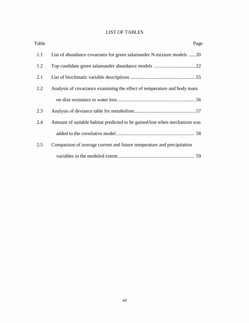
LIST OF TABLES

Table Page

1.1 List of abundance covariates for green salamander N-mixture models ...... 20

1.2 Top candidate green salamander abundance models .................................. 22

2.1 List of bioclimatic variable descriptions ..................................................... 55

2.2 Analysis of covariance examining the effect of temperature and body mass

on skin resistance to water loss ................................................................ 56

2.3 Analysis of deviance table for metabolism .................................................. 57

2.4 Amount of suitable habitat predicted to be gained/lost when mechanism was

added to the correlative model ................................................................ 58

2.5 Comparison of average current and future temperature and precipitation

variables in the modeled extent............................................................... 59

viii

LIST OF FIGURES

Figure Page

1.1 Map of study area in South Carolina .......................................................... 25

1.2 Habitat size and elevation as the top predictors of abundance ................... 26

2.1 Flowchart illustrating the inputs, process, and outputs of mechanistic

layers ..................................................................................................... 62

2.2 Effect of temperature on skin resistance to water loss ................................ 63

2.3 Effect of temperature on metabolism .......................................................... 64

2.4 Species distribution models for green salamanders .................................... 65

1

CHAPTER ONE

ENVIRONMENTAL PREDICTORS OF GREEN SALAMANDER DISTRIBUTION AND

ABUNDANCE IN THE BLUE RIDGE ESCARPMENT

INTRODUCTION

Amphibian habitat suitability can be constrained by a wide array of factors attributable to

natural habitat heterogeneity (Tockner et al. 1996; Vallan 2002) and anthropogenic changes such

as forest fragmentation and climate change (Petranka et al. 1993; Gibbs 1998; Araújo et al. 2006;

Barrett et al. 2014). Habitat specialists are particularly susceptible to factors altering distributions

at a wide range of spatial scales. Specialists suffer greater population declines when faced with

habitat loss and tend to be less resilient to the effects of climate change when compared to

generalists (Travis 2003; Munday 2004). Small-bodied specialists that live at higher elevations

and have limited ability to evade diseases, are at particularly high risk of extinction (Owens and

Bennett 2000; Pounds et al. 2006).

The Green Salamander, Aneides aeneus (Cope and Packard 1881), is considered a habitat

specialist and is the only member of the “climbing salamander” genus found on the east coast of

the United States. This species is typically associated with narrow granitic or sandstone rock

crevices (Bruce 1968; Mount 1975). Green Salamanders have specialized toe-tips which allow

them to climb up vertical surfaces and a unique lichen-like pattern on their dorsum that allows

them to blend in with their surroundings (Mount 1975; Petranka 1998). Green Salamanders occur

from southwestern Pennsylvania to northern Alabama and into eastern Mississippi. There is a

disjunct population in the Blue Ridge Escarpment (Petranka 1998). Green Salamanders are

considered “near threatened” by the International Union for Conservation of Nature (IUCN).

2

Within the disjunct Blue Ridge Escarpment (BRE) population, Green Salamanders are state

listed as “imperiled” in Georgia and North Carolina, and “critically imperiled” in South Carolina

(Natureserve 2017).

Snyder (1983) noted that Green Salamanders in the Carolinas are close to extinction.

Corser (2001) acknowledges four major threats facing Green Salamanders: habitat loss, climate

change, over-collection of the species, and disease. Little is known about Green Salamander

dispersal but it has been documented that they can disperse 42 m from the nearest rock outcrop

(Waldron and Humphries 2005). Thus researchers believe it is important to have forested buffers

around outcrops during clear-cutting (Petranka 1998; Wilson 2001; Waldron and Humphries

2005). The BRE has experienced warmer summer temperatures and colder winter temperatures

since the 1960’s, and like many other amphibians of high conservation priority, the Green

Salamander is expected to lose a significant amount of its climatically suitable habitat in the next

half-century (Snyder 1991; Corser 2001; Barrett et al. 2014). Nevertheless, the Carolinas have

been identified as an area of resilience to climatic change relative to many other parts of the

range (Barrett et al. 2014). Over-collection of Green Salamanders (which are highly coveted for

their attractiveness) could potentially lead to population declines (Corser 2001; Wilson 2001).

For example, continual collection of egg-brooding Green Salamanders from the same site over

consecutive years can result in population decline (Wilson 2001). Green Salamanders are likely

vulnerable to disease such as chytrid fungus because they occur in moist conditions at high

elevations (Daszak et al. 1999; Young et al. 2001). Recently, cases of chytrid fungus have been

detected in both Virginia and North Carolina and Ranavirus was reported in Virginia (Blackburn

et al. 2015; Moffitt et al. 2015).

3

With the growing threat of habitat loss and global climate change, I sought to determine

the current status of Green Salamanders within South Carolina. The last extensive inventories for

the species in the area were done in 1968 and 1990 (Bruce 1968; Hafer and Sweeney 1993).

These surveys identified different habitat affiliations; specifically, salamanders appeared more

frequently on south-facing slopes in the 1960s survey and a wider range of elevations (Bruce

1968), but more commonly on north-facing slopes and higher elevations in the Hafer and

Sweeney (1993) survey. It is an open question whether this is a real shift driven by temperature

or some other factor, or if it resulted from sampling error. To identify the current distribution and

status of Green Salamanders in the southern portion of the range, I sampled prospective Green

Salamander habitat in the Blue Ridge Mountains of South Carolina. I did so by reassessing

known historical Green Salamander localities and some newly located prospective sites in South

Carolina (sensu Corser 2001). I assessed a wide range of habitat features within and around sites

to evaluate potential predictors of site-level abundance. I also documented several new occupied

sites in South Carolina.

METHODS

Data Collection

I collected a comprehensive list of historical Green Salamander records in South Carolina

from the South Carolina Department of Natural Resources and three publically-accessible online

databases (Price and Dorcas 2007; Cicero et al. 2010; USGS 2013). I also identified potential

localities through conversations with South Carolina state park officials and through searching

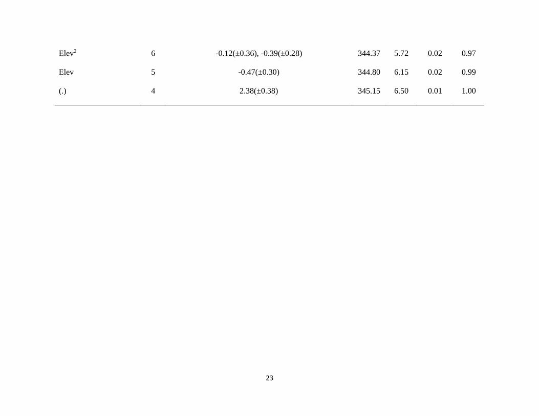
rock outcrops while traveling to historical locations. A total of 96 distinct sites were identified

within three counties containing the Blue Ridge Region of South Carolina (Fig. 1.1, inset map).

4

Thirty-five of these sites were not surveyed because sites had no rocky outcrops or large trees

with flaky bark that could be identified at the locale (n = 24), sites were inaccessible from roads

or trails (n=10), or sites were on private land that I did not have permission to access (n = 1).

For the remaining 61 accessible sites with appropriate habitat (an emergent rock outcrop), I

surveyed them three times each (with the exception of two sites which were only surveyed once

due to time constraints) between May and August 2016 (Hafer and Sweeney 1993; Corser 2001;

Waldron and Humphries 2005). Surveys were spread across the entire survey period with two

rounds of surveys conducted mid-morning to mid-day, and one round of surveys conducted at

dawn (no surveys were conducted at night due to logistical and safety concerns). Surveys were

done in a standardized fashion using a similar method outlined by Miloski (2010) by 1–2

observers depending on the rock outcrop size. I established circular plots around a rock outcrop

within historical Green Salamander sites and I created four 25–m transects representing the four

cardinal directions (N, E, S, and W). Each visit consisted of a two-part visual encounter survey

by the observer(s): (1) a thorough search of the entire rock outcrop using a headlamp, and (2) a

line-transect survey in which the observer(s) walked all four transects searching trees (2 m on

each side of the transect line) using binoculars and flipping cover objects checking for

salamanders. All herpetofauna encountered throughout surveys were recorded. I also collected

habitat variables during every survey (except for habitat size which was measured once),

assuming measurement error and thus taking an average measurement (Table 1.1). I measured

habitat size (outcrop size) by assuming the sites were roughly rectangular in shape, so I

multiplied the north-south and the east-west distance of the rock outcrop using a reel measuring

tape (Keson 300-ft Tape, Keson Industries, Inc.). I collected elevation using a Garmin GPS

(GPSmap 62s, Garmin, Ltd.), slope using a clinometer (PM5/1520, Suunto), and aspect using a

5

compass (MCB CM/IN/NH, Suunto). I assessed drainage presence/absence within 400 m of the

site based on a visual assessment and Google Earth (v7.1.8.3036, Google, Inc.), and land cover

within a 25-m radius of the outcrop was categorized as mixed forest, hardwood, softwood, or

shrub based on our observations during site visits. I measured basal area using a 10-factor prism

(Jim-Gem Square-shaped, Forestry Suppliers) and canopy cover (to the nearest 0.01) using a

concave densitometer (Spherical Crown, Forestry Suppliers) at the beginning of each of the four

line transects. I downloaded four bioclimatic variables (BIO1, BIO5, BIO12, BIO17) from

World Clim (Hijmans et al. 2005) and extracted the raster values to the Green Salamander

presence points in ArcMap (ArcGIS 10.3.1, ESRI). These data correspond to mean annual

temperature, maximum temperature of the warmest month, annual precipitation, and

precipitation of the driest quarter for the period 1960 – 1990.

Abundance Analysis

Using data from visual encounter surveys, I developed an N-mixture model for Green

Salamanders in South Carolina to investigate the relationships between species counts and

environmental site covariates. I analyzed count data using the unmarked package (Fiske and

Chandler 2011) in Program R 3.3.1 (R Core Team 2017). I used the “p-count” function to fit N-

mixture models to the count data. Abundance models assume that the population is closed and

counts between sites (rock outcrops) are independent of other sites. I assessed the weight of

evidence for a model using the Akaike’s Information Criterion (AIC). I standardized all

continuous covariates before putting them into the models and removed highly correlated

variables a priori. I transformed the aspect variable on a north/south gradient by taking the

absolute value of the difference of the aspect value and 180. The land cover variable was

6

removed from the analysis because there was only a small proportion of sites with softwood and

shrub-dominated habitats. The drainage variables were removed because all sites had a drainage

present within 400-m of the site. Bioclimatic variables were removed because each of the

measures had high pairwise correlation values with elevation (≥ ±0.96). I began by exploring

three possible model structures on the null model: negative binomial, zero-inflated Poisson, and

Poisson. A comparison of these structures via AIC revealed the most support for the negative

binomial, so all subsequent models were created with this structure.

I first identified survey-specific covariates that may have influenced detection probability

(observer experience, total search time, time of day, cloud cover, temperature, and Julian

calendar day number). Observers were given a ranking between 0–2 (“0” referred to a low level

of experience and “2” referred to a high level of experience). Observers new to the field or naïve

to field equipment were designated as having less experience than those observers who have had

3+ years in the field and have worked with a variety of field equipment. With time, less

experienced observers became more experienced and earned a ranking of “2” as the field season

progressed. If multiple observers were conducting the survey, then their experience score was

averaged. Total search time was measured as the amount of time it took the observer(s) to

complete a survey effort, and I divided this measure by total habitat size to generate the search

effort variable (hereafter, “duration”). Time of day was included because searches ranged from

dawn to mid-day. Cloud cover was broken up into two categories: overcast and sunny. Rain

events were considered overcast. I took air temperature using a thermometer (6-1/4” Pocket Case

Enviro-Safe, Forestry Suppliers). I recorded the Julian day number based on the 2016 leap year

calendar.

7

I began identifying possible covariates of detection by comparing a null model to all possible

univariate models of detection covariates, while keeping abundance covariates constant across

sites. Detection covariates with strong support (AIC < 2) were evaluated in all possible

combinations to explore support for additive models. Once I determined which detection model

had the most support (∆AIC = 0), I incorporated this detection covariate model in all subsequent

models exploring covariates of abundance. Similar to our process for identifying detection

covariates, I first generated all possible univariate models with abundance covariates, identified

those variables with the most support (AIC < 4; which also represented weights >0.1), and then

examined all possible combinations of those covariates. Our final model comparison (via AIC)

involved the null model, strongly supported univariate models, and all possible multivariate

models involving the top abundance covariates.

RESULTS

Distribution and Arboreal Use

Out of the 61 sites that I surveyed, 30 had Green Salamander detections (49.1%). Ten of

those sites were new potential Green Salamander locales in the South Carolina Blue Ridge

region. These new locales were located in Pickens County, SC (n=7) and Oconee County, SC

(n=3). The majority of these sites were south-facing (n=8), ranged in elevation from 399–641 m,

and in size from 136–6649 m2. Out of the ten newly discovered potential sites that I surveyed,

seven had detections (70%). I found six Green Salamanders using arboreal habitats during

surveys. In addition, I found six salamanders (three on one occasion) on a Red Oak, Quercus

falcata, at Table Rock State Park that was not in a survey plot. The farthest distance I

documented a Green Salamander from a rock outcrop to an arboreal habitat was 35.2 m. The

8

highest observation of a Green Salamander on a tree was approximately 9 m from the ground on

a mossy patch of a Red Oak. Green Salamanders were documented on hardwoods including Red

Oaks, Red Maples (Acer rubrum), Black Cherries (Prunus serotina) as well as other

arboreal/woody habitats such as rotten logs and tree snags.

Detection and Abundance Analyses

Time of day emerged as the most important variable for detecting Green Salamanders.

Detection probability of Green Salamanders across all sites and across sites known to be

occupied ranged from ~0.03 – 0.13 as a function of time of day. Salamanders had a higher

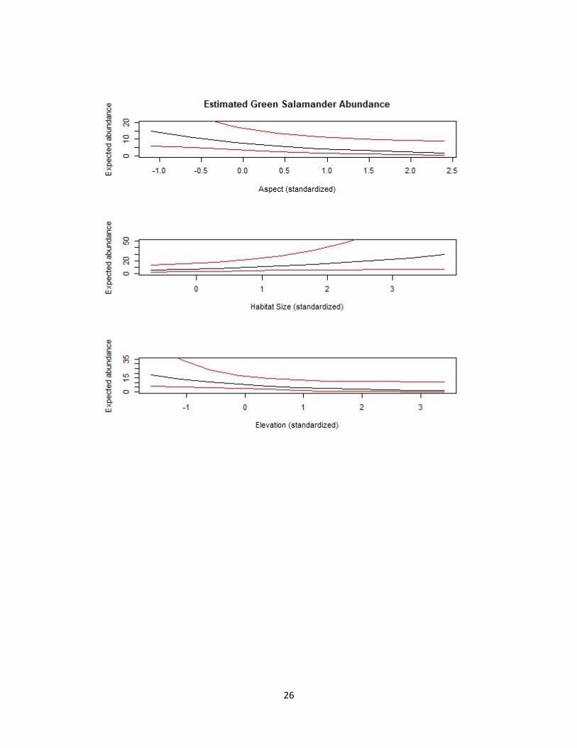
probability of being detected later in the day. Aspect, size, and elevation were the only three

variables that were supported among our candidate set of abundance covariates (Table 1.2). The

top candidate model contained all three abundance covariates – aspect, habitat size, and elevation

(in its linear form; Table 1.2). There were also two other models with a ∆AIC <2 and therefore,

had some support in my analysis (Table 1.2). In the second top model (Aspect+Size), parameter

estimates for both aspect and size were similar for both models and so this second model is not

adding any new additional information to my analysis. In the third top model

(Apsect+Size+Elev2 model), the quadratic term crosses zero and thus is not an informative term.

Aspect had a negative influence on Green Salamander abundance and size had a positive

influence on abundance (Table 1.2; Fig. 1.2). I found support for models where elevation had a

direct negative on abundance (Table 1.2; Fig. 1.2), however, the quadratic effect was not

informative (Table 1.2). Out of the 51 historical locations that I surveyed, 23 of these sites had

detections. I adjusted for detection probability by using what I know about aspect, habitat size,

and elevation at a site to predict abundance at a particular site and determined that 45/51

9

(88.24%) historical sites that I surveyed were predicted to have at least two individual green

salamanders. I used two individuals as the threshold because that was my estimate of abundance

at the least-abundant site with confirmed occupancy. For a survey of average habitat size and

elevation, abundance increased by ~4.7-fold (from 1.72 to 8.08) as aspect shifted from more

northerly- to southerly-facing sites. For a survey of average aspect and elevation, abundance

increased by ~5-fold (from 5.93 to 29.24) as habitat size ranged from approximately 1–6650 m2.

For a survey of average aspect and habitat size, abundance increased by ~15-fold (from 1.21 to

18.06) as elevation ranged from approximately 280-1040 m.

DISCUSSION

Green Salamander abundance was influenced by aspect, habitat size, and elevation (Table

1.2; Fig 1.2). Interestingly, sites with south-facing slopes (which tend to be xeric) had higher

estimated abundances of Green Salamanders than those with north-facing slopes. This is

consistent with Bruce (1968) who suggests that rock outcrops sites on south-facing slopes may

be buffered from sunlight penetration because of the narrowness and irregularity of the crevices

in which Green Salamanders are found in. Our findings, however, are inconsistent with more

recent literature suggesting a preference for northerly-facing slopes (Hafer and Sweeney 1993).

Hafer and Sweeney (1993) based their criteria for “high probability of containing suitable Green

Salamander habitat” off of 14 known Green Salamander locales (with ten of those sites having a

northerly-facing aspect), thus it is likely this small sample size may have biased their

conclusions. As expected, larger sites had higher estimated abundances of salamanders than

smaller sites. Larger sites represent opportunities for higher Green Salamander numbers and thus

contribute to genetic diversity (Petranka et al. 1993; Noël et al. 2007). The model with the most

10

support indicated a negative relationship between estimated abundance and elevation, however

the quadratic elevation covariate was uninformative (Table 1.2). A study in Ohio suggested that

Green Salamanders preferred low elevations between 183–244 m (Lipps 2005). The Bruce

(1968) Green Salamander surveys characterized rock outcrop sites in the BRE to have a wide

elevational range, including low elevations (305-m and above). He suggests that although higher

elevations may be available to salamanders in the BRE, they may not be able to disperse to them

because of the topography. Further, salamanders may prefer the stable microclimates provided

by lower elevation gorges of the BRE (Bruce 1968). Hafer and Sweeney (1993) characterized

habitat suitability of Green Salamanders in South Carolina to increase with elevation, which is

contrary to our findings. Knowledge of site-specific population growth rates and genetic

diversity would be valuable contributions toward further contextualizing the environmental

associations I describe here.

Detection of Green Salamanders was influenced by time of day in an unexpected manner.

Surprisingly, time of day had a positive influence on detection of salamanders suggesting that

salamanders were more surface active (and therefore easier to detect) later in the day. In other

words, Green Salamanders were more detectable during the hotter parts of the days. Rock

outcrop microclimate is likely buffered from the surrounding warm and dry air associated with

the hottest times of the day (Locosselli et al. 2016). Several findings within this study and others

suggest Green Salamanders in the BRE may be somewhat resilient to warm and dry conditions

(Gordon 1952; Bruce 1968; Barrett et al. 2014). For example, one preliminary laboratory study

documented Green Salamanders to have a higher tolerance to drying compared to another

plethodontid salamander, Plethodon metcalfi (=Plethodon jordani melavantris) (Gordon 1952).

11

This suggests that Green Salamanders may be able to take advantage of sites that are less suitable

for other species using rock outcrops (e.g., Plethodon metcalfi).

Many of the historical localities in South Carolina that I surveyed fell short of the suggested

100-m forested buffer (Petranka 1998; Wilson 2001; Waldron and Humphries, 2005). For

example, fourteen rock outcrop sites had < 20 m of forest between the site and a paved road or

powerline cut (eight of which were occupied). Throughout surveys, I only saw six salamanders

within arboreal habitats. Occupied trees were predominately hardwoods, similar to those found

in the Waldron and Humphries (2005), however two detections were found on rotten logs/tree

snags. The majority of detections outside of rocky outcrops occurred on moss, lichen, or flaky

bark which likely provide moist refugia. Our farthest documented movement during the survey

season was 35 m from the nearest rock outcrop and therefore it is likely that some salamanders at

these sites are exposed to a lack of shade due to open canopy. Detections away from rock

outcrops may have been influenced by the extreme drought (in part from the 2016 El Niño

event), which could have decreased movements away from moist rock crevices. Furthermore,

many sites had a thick Rhododenron understory so it is possible that I missed detections in this

thick shrub. Rhodoendron detections were high in North Carolina Green Salamander surveys

(pers. communication, M. Hall). Open canopies have been found to limit migration opportunities

and lead to patchy distributions (Gordon 1952; Snyder 1991; Corser 2001), but I do not have

data on movement among the habitats studied here.

Green Salamanders were detected in less than half of the sites that I surveyed and when they

were detected, they were not typically abundant (Fig 1.1, main map). When I adjusted for

detection probability, six sites were predicted to have less than two individual Green

Salamanders. Three of these sites were located in Greenville County, two of these sites were in

12

Pickens County, and one of these sites was in Oconee County. Because the species has low

detection probability it is possible that some sites were occupied even though I never detected

individuals. Nevertheless, our survey methods represent a more intensive survey effort than

either of the two previous surveys in South Carolina (Bruce 1968; Hafer and Sweeney 1993).

Future status assessments should explore ways to increase detection of individuals by

incorporating fall (September and October) and nighttime salamander surveys. Knowledge of

distributional shifts relative to historical trends will allow for a better understanding of how

Green Salamanders will respond to threats such as land use and climate change, as well as

disease and collection.

MANAGEMENT RECOMMENDATIONS

Current Habitat Protection

My results suggest that aspect, habitat size, and elevation have the most influence on Green

Salamander abundance. In order to protect current Green Salamander habitat, it would be

beneficial to focus on protecting bigger rocky outcrop sites at lower elevations on south-facing

slopes (as these were the habitat associations that predicted highest abundances). Although

south-facing slopes are known to be xeric, literature suggests that the rock crevices in which

Green Salamanders are found in are structured in such a way that they deflect sunlight (Bruce

1968). Additionally, larger habitats (rock outcrops) are likely important for this habitat specialist

because they provide additional refugia for salamanders to be active (i.e. foraging and

reproduction) and this can lead to increased genetic diversity (Petranka et al. 1993; Noël et al.

2007). Further, the results of my study along with others suggest that Green Salamanders prefer

lower elevations (Bruce 1968; Lipps 2005). Literature suggests that the microclimate at lower

13

elevations may be preferential to Green Salamanders and additionally, salamanders may not be

able to access higher elevations due to limitations in dispersal (Bruce 1968).

Determining Occupancy

Detection of Green Salamanders in South Carolina was most influenced by time of day in

which surveys were conducted. Unexpectedly, my results suggested that Green Salamanders

were more easily detected later in the day. Therefore, I recommend surveying Green

Salamanders mid-day. Although observer did not emerge as a detection covariate, I strongly

recommend developing a search image of the species before conducting surveys. Green

Salamanders are known to be a cryptic species and thus having a search image for the species

will greatly increase an observer’s odds of seeing a camouflaged salamander in its habitat. In

order to develop a search image, I recommend all surveys have previous experience or gain

experience by working with a trained individual.

When conducting visual encounter surveys for Green Salamanders, I recommend visiting

a site three times in order to determine whether or not a site is occupied. Three visits to a site

provides sufficient data to make an informative decision about a particular site. The top model

suggests a 10% chance of detecting a salamander and so if a site has at least ten salamanders, an

observer is likely to detect at least one of them on a single visit (if the highest detection

probability is assumed). Further, I also suggest spreading visits throughout the Green

Salamander’s active season (Gordon 1952). Green Salamanders come out of hibernation starting

in late April, breed from May – September, and finally have a period of dispersal/aggregation

before hibernating in November (Gordon 1952).

14

Logging Management on Public Property

Of the 61 surveyed Green Salamander sites that I surveyed, there were 14 localities with

< 20 m of a forested buffer between the rock outcrop site and a landscape disturbance (paved

road or powerline cut). Sites without a forested buffer were expected to have fewer salamanders

per site (8.82 ± 6.10) compared to sites with a forested buffer (11.66 ± 8.63). During the survey

season, I documented a Green Salamander 35 m away from the nearest rock outcrop and the

longest documented movement from a rock outcrop to a tree is 42 m (Waldron and Humphries

2005). In previous literature, scientists have suggested a 100-m forested buffer around rock

outcrops (Petranka 1998; Wilson 2001; Waldron and Humphries, 2005). I strongly agree with

this recommendation as this is a seasonally arboreal species that likely spends significant

amounts of time in trees (Waldron and Humphries 2005).

15

REFERENCES

Araújo, M. B., W. Thuiller, and R. G. Pearson. 2006. Climate warming and the decline of

amphibians and reptiles in Europe. Journal of Biogeography 33:1712–1728.

Barrett, K., N. P. Nibbelink, and J. C. Maerz. 2014. Identifying priority species and conservation

opportunities under future climate scenarios: Amphibians in a biodiversity hotspot.

Journal of Fish and Wildlife Management 5:282–297.

Blackburn, M., J. Wayland, W. H. Smith, J. H. McKenna, M. Harry, M. K. Hamed, M. J. Gray,

D. L. Miller. 2015. First report of Ranavirus and Batrachochytrium dendrobatidis in

green salamanders (Aneides aeneus) from Virginia, USA. Herpetological Review

46:357–361.

Brodman, R. 2004. R9 species conservation assessment for the green salamander, Aneides

aeneus (Cope and Packard). Conservation Assessment 1–17.

Bruce, R. C. 1968. The role of the Blue Ridge Embayment in the zoogeography of the green

salamander, Aneides aeneus. Herpetologica 24:185–194.

Cicero, C., H. Bart, D. Bloom, R. Guralnick, M. Koo, J. Otegui, N. Rios, L. Russell, C. Spencer,

D. Vieglais, J. Wieczorek,. 2010. VertNet: an online reference Available at:

http://www.vertnet.org/index.html. Archived by WebCite at

http://www.webcitation.org/6pD7hOsZF on 24 March 2017.

Cope, E. D., A. S. Packard. 1881. The fauna of the Nickajack Cave. American Naturalist

15:877–882.

Corser, J. D. 2001. Decline of disjunct green salamander (Aneides aeneus) populations in the

southern Appalachians. Biological Conservation 97:119–126.

Corser, J. D. 1991. The Ecology and Status of the Endangered Green Salamander (Aneides

16

aeneus) in the Blue Ridge Embayment of North Carolina. Master’s Thesis. Duke

University, Durham, North Carolina, United States of America.

Daszak, P., L. Berger, A. A. Cunningham, A. D. Hyatt, D. E. Green, and R. Speare. 1999.

Emerging infectious diseases and amphibian population declines. Emerging Infectious

Diseases 5:735–748.

Fiske, I., R. Chandler. 2011. unmarked: An R package for fitting hierarchical models of wildlife

occurrence and abundance. Journal of Statistical Software 43:1-23.

Gibbs, J. P. 1998. Distribution of woodland amphibians along a forest fragmentation gradient.

Landscape Ecology 13:263-268.

Gordon, R. E. 1952. A contribution to the life history and ecology of the plethodontid

salamander Aneides aeneus (Cope and Packard). The American Midland Naturalist

47:666–701.

Hafer, M. L. A., J. R. Sweeney. 1993. Status of the green salamander in South Carolina.

Proceedings of the Annual Conference of Southeastern Association of Fish and Wildlife

Agencies 47:414–418.

Hijmans, R. J., S. E. Cameron, J. L. Parra, P. G. Jones, A. Jarvis. 2005. Very high resolution

interpolated climate surfaces for global land areas. International Journal of Climatology

25: 1965–1978.

Lipps, Jr. G. J. 2005. A Framework for Predicting the Occurrence of Rare Amphibians: A Case

Study with the Green Salamander. Master’s Thesis. Bowling Green State University,

Bowling Green, Ohio, United States of America.

Locosselli, G. M., R. H. Cardim, G. Ceccantini. 2016. Rock outcrops reduce temperature-

induced stress for tropic conifer by decoupling regional climate in the semiarid

17

environment. International Journal of Biometeorology 60:639-649.

Miloski, S. E. 2010. Movement Patterns and Artificial Arboreal Cover Use of Green

Salamanders (Aneides aeneus) in Kanawha County, West Virginia. Master’s Thesis.

Marshall University, Huntington, West Virginia, United States of America.

Moffitt, D., L. A. Williams, A. Hastings, M. W. Pugh, M. M. Gangloff, and L. Siefferman. 2015.

Low prevalence of the amphibian pathogen Batrachochytrium dendrobatidis in the

southern Appalachian mountains. Herpetological Conservation and Biology 10:123–

136.

Mount, R. H. 1975. The Reptiles and Amphibians of Alabama. Alabama, United States of

America.

Munday, P. L. 2004. Habitat Loss, resources specialization, and extinction on coral reefs. Global

Change Biology 10:1642–1647.

Natureserve. 2017. NatureServe Explorer: an online encyclopedia of life [web application].

Version 7.0. NatureServe, Arlington, VA. U.S.A. Available

at http://explorer.natureserve.org. Archived by WebCite at

http://www.webcitation.org/6pEaNoD3E on 25 March 2017.

Noël, S., M. Ouellet, P. Galois, F. J. Lapointe. 2007. Impact of urban fragmentation on the

genetic structure of the eastern red-backed salamander. Conservation Genetics 8:599–

606.

Owens, I. P. F. and P. M. Bennett. 2000. Ecological basis of extinction risk in birds: habitat loss

versus human persecution and introduced predators. Proceedings of the National

Academy of Sciences of the U. S. A. 97:12144–12148.

Petranka, J. W., Eldridge M. E., Haley, K. E. 1993. Effects of timber harvesting on southern

18

Appalachian salamanders. Conservation Biology 7:363–370.

Petranka, J. W. 1998. Salamanders of the United States and Canada. United States of America.

Pounds, J. A., M. R. Bustamante, L. A. Coloma, J. A. Consuegra, M. P. Fogden, P. N. Foster, E.

La Marca, K. L.Masters, A.Merino-Viteri, R. Puschendorf, S. R. Ron, G. A. Sanchez-

Azofeifa, C. J. Still, and B. E. Young. 2006. Widespread amphibian extinctions from

epidemic disease driven by global warming. Nature 439:161–167.

Price, S. J., M. E. Dorcas. 2007. Carolina Herp Atlas: an online reference Available at

https://www.carolinaherpatlas.org/. Archived by WebCite at

http://www.webcitation.org/6pD5Mcnyp on 24 March 2017.

Snyder, D. H. 1991. The green salamander (Aneides aeneus) in Tennessee and Kentucky, with

comments on the Carolinas’ Blue Ridge populations. Journal of the Tennessee Academy

of Science 66:165–169.

Snyder, D. H. 1983. The apparent crash and possible extinction of the green salamander, Aneides

aeneus, in the Carolinas. Association of Southeastern Biologists Bulletin 30:82.

Spickler, J. C., S. C. Sillett, S. B. Marks, and H. H. Welsh, Jr. 2006. Evidence of a new niche for

a North American salamander: Aneides vagrans residing in the canopy of old-growth

redwood forest. Herpetological Conservation and Biology 1:16–26.

Travis, J. M. J. 2003. Climate change and habitat destruction: a deadly anthropogenic cocktail.

Proceedings of the Royal Society of London 270:467–473.

Tockner, K., F. Schiemer, C. Baumgartner, G. Kum, E. Weigand, I. Zweimuller, J. V. Ward.

1999. The Danube restoration project: species diversity patterns across connectivity

gradients in the floodplain system. Regulated Rivers-Research and Management 15:245–

258.

19

USGS. 2013. Biodiversity Information Serving Our Nation (BISON): an online reference

Available at https://bison.usgs.gov/#home. Archived by WebCite at

http://www.webcitation.org/6pD6JtGpT on 24 March 2017.

Vallan, D. 2002. Effects of anthropogenic environmental changes on amphibian diversity in the

rain forests of eastern Madagascar. Journal of Tropical Ecology 18:725–742.

Waldron, J. L. and W. J. Humphries. 2005. Arboreal habitat use by the green salamander,

Aneides aeneus, in South Carolina. Journal of Herpetology 39:486–492.

Wilson, C. R. 2001. Green Salamander, Aneides aeneus. Chattooga Quarterly: Spring/Summer

2001 Edition 3–4.

Young, B. E., K. R. Lips, J. K. Reaser, R. Ibanez, A. W. Salas, J. R. Cedeno, L. A. Coloma, S.

Ron, E. La Marca, J R. Meyer, A. Munoz, F. Bolanos, G. Chaves, and D. Romo. 2001.

Population declines and priorities for amphibian conservation in Latin America.

Conservation Biology 15:1213–1223.

20

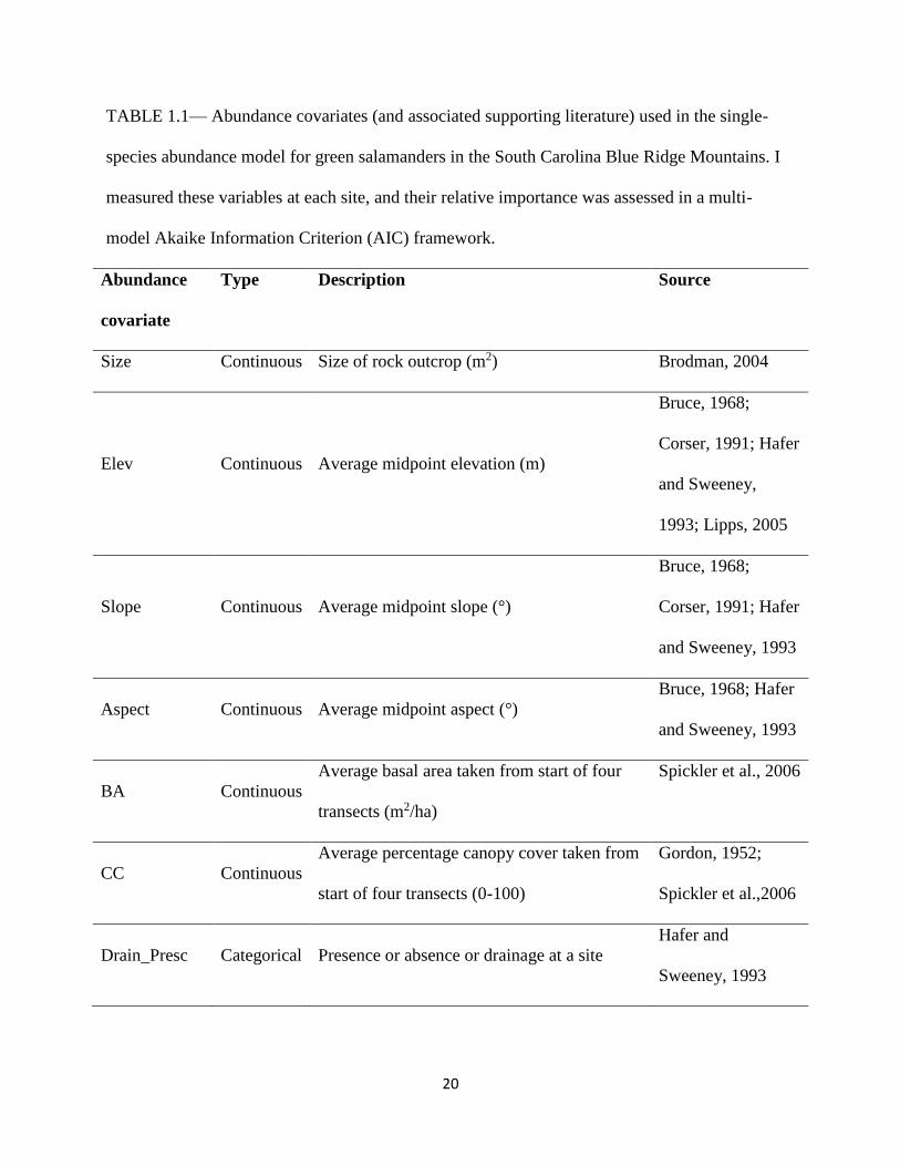
TABLE 1.1— Abundance covariates (and associated supporting literature) used in the single-

species abundance model for green salamanders in the South Carolina Blue Ridge Mountains. I

measured these variables at each site, and their relative importance was assessed in a multi-

model Akaike Information Criterion (AIC) framework.

Abundance

covariate

Type Description Source

Size Continuous Size of rock outcrop (m2) Brodman, 2004

Elev Continuous Average midpoint elevation (m)

Bruce, 1968;

Corser, 1991; Hafer

and Sweeney,

1993; Lipps, 2005

Slope Continuous Average midpoint slope (°)

Bruce, 1968;

Corser, 1991; Hafer

and Sweeney, 1993

Aspect Continuous Average midpoint aspect (°)

Bruce, 1968; Hafer

and Sweeney, 1993

BA Continuous

Average basal area taken from start of four

transects (m2/ha)

Spickler et al., 2006

CC Continuous

Average percentage canopy cover taken from

start of four transects (0-100)

Gordon, 1952;

Spickler et al.,2006

Drain_Presc Categorical Presence or absence or drainage at a site

Hafer and

Sweeney, 1993

21

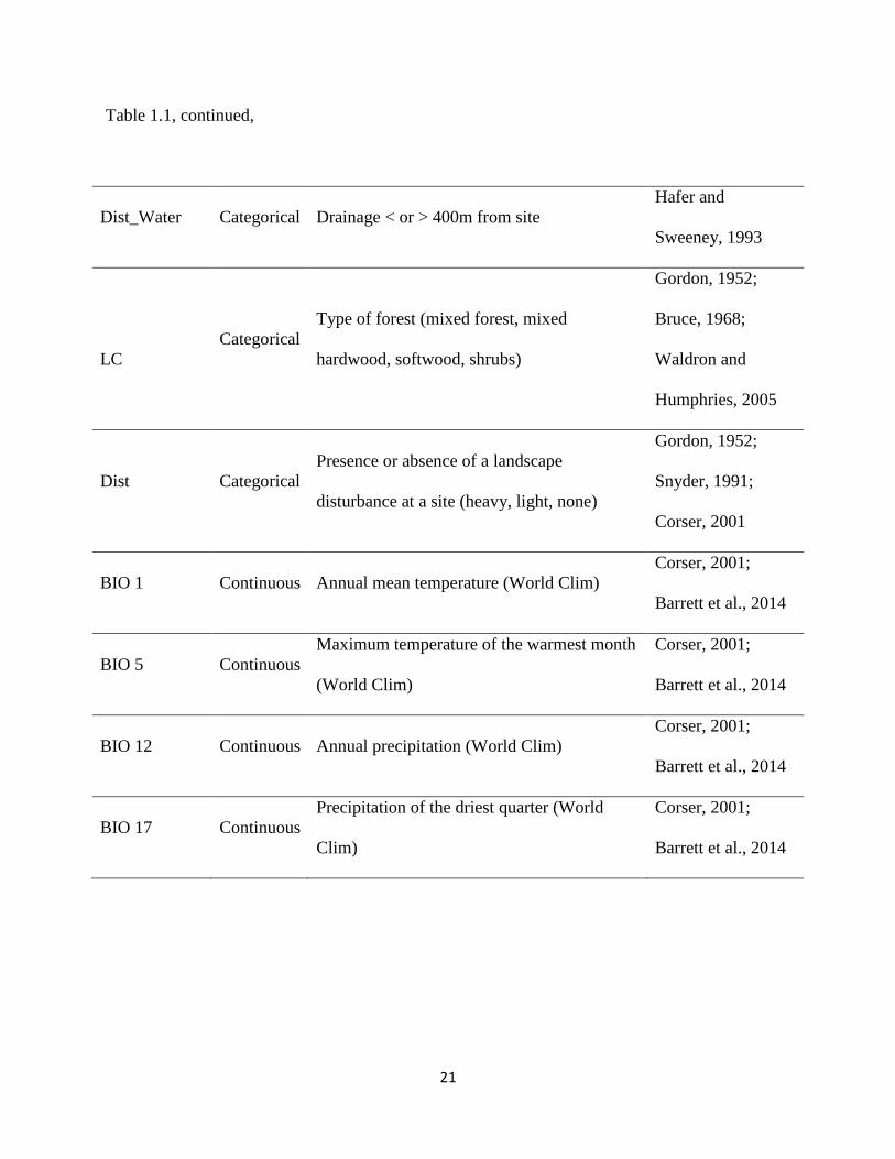
Table 1.1, continued,

Dist_Water Categorical Drainage < or > 400m from site

Hafer and

Sweeney, 1993

LC

Categorical

Type of forest (mixed forest, mixed

hardwood, softwood, shrubs)

Gordon, 1952;

Bruce, 1968;

Waldron and

Humphries, 2005

Dist Categorical

Presence or absence of a landscape

disturbance at a site (heavy, light, none)

Gordon, 1952;

Snyder, 1991;

Corser, 2001

BIO 1 Continuous Annual mean temperature (World Clim)

Corser, 2001;

Barrett et al., 2014

BIO 5 Continuous

Maximum temperature of the warmest month

(World Clim)

Corser, 2001;

Barrett et al., 2014

BIO 12 Continuous Annual precipitation (World Clim)

Corser, 2001;

Barrett et al., 2014

BIO 17 Continuous

Precipitation of the driest quarter (World

Clim)

Corser, 2001;

Barrett et al., 2014

22

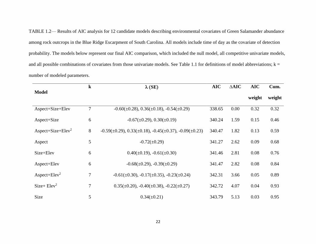
TABLE 1.2— Results of AIC analysis for 12 candidate models describing environmental covariates of Green Salamander abundance

among rock outcrops in the Blue Ridge Escarpment of South Carolina. All models include time of day as the covariate of detection

probability. The models below represent our final AIC comparison, which included the null model, all competitive univariate models,

and all possible combinations of covariates from those univariate models. See Table 1.1 for definitions of model abbreviations; k =

number of modeled parameters.

Model

k

SE AIC ∆AIC AIC

weight

Cum.

weight

Aspect+Size+Elev 7 -0.60(±0.28), 0.36(±0.18), -0.54(±0.29) 338.65 0.00 0.32 0.32

Aspect+Size 6 -0.67(±0.29), 0.30(±0.19) 340.24 1.59 0.15 0.46

Aspect+Size+Elev2 8 -0.59(±0.29), 0.33(±0.18), -0.45(±0.37), -0.09(±0.23) 340.47 1.82 0.13 0.59

Aspect 5 -0.72(±0.29) 341.27 2.62 0.09 0.68

Size+Elev 6 0.40(±0.19), -0.61(±0.30) 341.46 2.81 0.08 0.76

Aspect+Elev 6 -0.68(±0.29), -0.39(±0.29) 341.47 2.82 0.08 0.84

Aspect+Elev2 7 -0.61(±0.30), -0.17(±0.35), -0.23(±0.24) 342.31 3.66 0.05 0.89

Size+ Elev2 7 0.35(±0.20), -0.40(±0.38), -0.22(±0.27) 342.72 4.07 0.04 0.93

Size 5 0.34(±0.21) 343.79 5.13 0.03 0.95

23

Elev2 6 -0.12(±0.36), -0.39(±0.28) 344.37 5.72 0.02 0.97

Elev 5 -0.47(±0.30) 344.80 6.15 0.02 0.99

(.) 4 2.38(±0.38) 345.15 6.50 0.01 1.00

24

FIG 1.1 —The inset map at the top represents the counties within South Carolina known

to contain Green Salamander localities. From left to right the shaded polygons are

Oconee, Pickens, and Greenville Counties. The main map shows the known distributional

range of Green Salamanders, Aneides aeneus, in upstate South Carolina. The light gray

polygon represents the historic range and the dark gray polygon represents the range based on

sites with confirmed presence from this study. Polygons were created using minimum

boundary geometry in ArcGIS. White circles represent sites that did not have suitable

habitat and black circles represent sites that were not accessible due to terrain. The

question mark represents the site that I did not have permission to access.

FIG 1.2—Aspect, habitat size, and elevation emerged as the best predictors of abundance

for Green Salamanders (Aneides aeneus) in South Carolina (Table 1.2). The top panel is

illustrating the effect of aspect on the estimated abundance of Green Salamanders when

both habitat size and elevation are held at their mean values. The middle panel is

illustrating the effect of size on the estimated abundance of Green Salamanders when

both aspect and elevation are held at their mean values. The bottom panel is illustrating

the effect of elevation on the estimated abundance of Green Salamanders when both

aspect and habitat size are held at their mean values. All panels have 95% CI.

25

26

27

CHAPTER TWO

ADDING MECHANISM TO A DISTRIBUTION MODEL CHANGES PREDICTIONS

OF CLIMATE VULNERABILITY FOR A PRIORITY AMPHIBIAN

INTRODUCTION

Understanding species response to global climate change will allow for more

informed conservation and management decisions. Climate change has been implicated

in population declines of several species (Both et. al. 2006; Carpenter et. al. 2008) and

disruptions in behavior for others. For example, avian and anuran species have shifted

their breeding seasons due to changes in temperature (Brown & Bhagabati 1999;

Barbraud & Weimerskirch 2006; Kusano & Inoue 2008). Further, it has been projected

that many European herpetofaunal species with limited dispersal will lose suitable habitat

in the future (Araújo et al. 2006), which may lead to population declines for additional

species.

A wide range of tools are available to forecast species response to climate change

(Füssel & Klein 2006; Butchart et al. 2010; Sutton et al. 2015). Among the available

tools, species distribution models provide spatially explicit models of vulnerability and

resilience. While the maps produced from such models offer conservation practitioners

guidance on where to exert efforts, there are important caveats associated with many of

the distribution modeling approaches (Buckley et al. 2010; Barrett et al. 2014; Roach et

al. 2017). Specifically, correlative models, which examine the association between

climatic variables and species locality data (Kearney et al. 2010; Barrett et al. 2014)

28

assume some underlying relationship between environmental conditions and the

distribution of the animal. Importantly, a physiological connection between these two

variables is not explicitly evaluated. As a result, the models may do a poor job projecting

habitat suitability in environments outside the range of the training data (Elith et al. 2010;

Milanovich et al. 2010). Mechanistic models offer an alternative approach to distribution

modeling. These models estimate animal performance (e.g., active foraging time or

reproduction) across habitats using empirically-derived relationships between animal

physiology and environmental conditions. Once these relationships are known, the

distribution of an organism can be mapped onto a range of environmental conditions

(Mathewson et al. 2017; Riddell et al. 2017). Research suggests that mechanism can

enhance correlative models when predicting climatically suitable habitat for a species

(Mathewson et al. 2017; Riddell et al. 2017); however, a recent review demonstrated few

mechanistic models in literature (Urban et al. 2016). The rarity of these models may

result from the data required to build them (i.e., experimentally-derived estimates of

animal physiology under a range of environmental conditions); nevertheless, several

examples of such models do exist – especially for ectotherms (Buckley 2008; Kolbe et al.

2010; Buckley et al. 2010; Riddell et al. 2015; Riddell et al. 2017).

I used green salamanders, Aneides aeneus (Cope & Packard 1881), to assess the

influence of adding mechanistic parameters to climate-based distribution models. Green

salamanders have experienced population declines in the disjunct portion of their range

(North Carolina, South Carolina, and Georgia) beginning in the 1970’s (Snyder 1983,

Corser 2001). In addition to habitat loss, over-collection, and disease, climate change has

29

also been implicated as a threat to this species (Corser 2001). Several correlative models

have been applied to green salamanders in all or parts of their range (Lipps 2005; Barrett

et al. 2014; Hardman 2014). These correlative models have helped determine habitat

associations and document new sites in areas where green salamanders are listed as

“endangered.” Additionally, the mid-century and end-of-century predictions of habitat

suitability from these models will aid in conservation-based decisions.

Currently, there are no mechanistic models for green salamander distribution.

However, Gordon (1952) conducted preliminary experiments examining vital limits of

green salamanders during water loss trials. Experiments compared physiological response

to drying under one temperature (20°C) treatment with dry air conditions between green

salamanders and Plethodon metcalfi (=Plethodon jordani melavantris). The study found

that green salamanders withstood drying longer than Plethodon metcalfi and thus on

average lost more water than Plethodon metcalfi. While the sample size was limited for

this study (N=15 green salamanders, N=7 Plethodon metcalfi), these results suggest that

green salamanders are likely able to withstand physiological challenges (such as

increased temperature) better than closely related species.

For this study, I used program MaxEnt (Maximum Entropy), a method for modeling

species distributions using presence-only data (Phillips et al. 2006). MaxEnt is used to

estimate the species distribution by finding the largest spread (maximum entropy) of a

geographic dataset containing presence data with association to environmental variables.

This program has been used to model suitable habitat of many species, particularly

amphibians that are globally-threatened or extinct (Baillie et al. 2004; Milanovich et al.

30

2010; Barrett et al. 2014; Hardman 2014; Sutton et al. 2015). I modeled suitable climatic

habitat for green salamanders throughout their disjunct range. I coupled physiological

data (resistance to water loss and metabolic rates) with climatic data to create a

mechanistic model for green salamanders. I compared the correlative models with and

without a mechanistic layer to evaluate model predictions under different climatic

scenarios.

METHODS

Salamander Care and Collection

I conducted experiments on green salamanders to evaluate the thermal sensitivity of

water loss rates and metabolic rates (Fig 2.1). I collected 2-6 green salamanders (avoiding

nesting and gravid females as well as juveniles) from four sites in South Carolina (N=19)

at night from April – May 2017. Sites were located in Table Rock State Park and Nine

Times Forest (precise locality withheld due to conservation concerns). These sites were

selected because previous surveys suggested animal densities were high enough to

provide sufficient captures for our trials without compromising the population.

Salamanders were transported in Ziploc bags (with moist leaf litter) to Clemson

University and placed in an incubator (15°C). Salamanders acclimated in individual

Ziploc containers with a wet paper towel for five days to ensure that physiological

measurements occurred during a post-absorptive state. As part of our animal care

protocol, I estimated a baseline mass (to the nearest 0.001 g) at the beginning of the

31

experiment to ensure that salamanders did not lose more than 10% of their baseline mass

while in the laboratory. Salamanders that did not maintain a baseline mass were excluded

from the experiment (see below). After the acclimation period, I measured water loss

rates and metabolic rates using a flow through system. All experiments were approved by

the Institute for Animal Care and Use Committee at Clemson University (AUP 2016-

035), and approval for collections and experimentation were granted by the South

Carolina State Park Service and the South Carolina Department of Natural Resources.

After the experimental trials, all collected animals were returned to capture sites.

Flow through system and physiological measurements

I measured the thermal sensitivity of water loss rates and metabolic rates using a flow

through system. Our system continuously exposed salamanders to highly controlled

temperature and humidity environments and simultaneously measured their physiology. I

controlled the environmental temperature using a programmable incubator (Percival

VL36). The system used a sub-sampler (SS-4; Sable Systems International (SSI)) to push

air through a dewpoint generator (DG-4; SSI) controlling the vapor pressure deficit

(VPD; the difference between the amount of moisture in the air and the amount of

moisture the air can hold). A flow manifold (MF-8; SSI) was then used to divide the

airstream into the individual cylindrical acrylic chambers. The chambers (16cm x 3.5cm;

volume ~ 153 mL) contained an individual green salamander placed on hardwire mesh to

expose its surface to the airstream (simulating posture during activity). I cycled air

between each chamber three times every ten minutes using a multiplexer (M8; SSI). The

32

airstream was then sampled using a vapor analyzer (RH-300; SSI) which measured the

change in water vapor pressure (kPa). Then, the air was scrubbed of water vapor and

carbon dioxide using Drierite (W. A. Hammond Drierite Co. Ltd.) and soda lime,

respectively. After scrubbing, I measured the partial pressure of oxygen using Oxzilla

(SSI).

I moved the individual Ziploc containers to an environmental chamber set to a

regulated experimental temperature (12°C, 18°C, 24°C) two hours prior to measuring

water loss rates. These temperatures were chosen to reflect the temperatures that green

salamanders would experience in nature during their active season (April - October;

Gordon 1952). I calculated skin resistance to water loss of green salamanders using a

combination of one of the three treatment temperatures (12°C, 18°C, 24°C) and a single

VPD (0.5 kPA). This VPD was chosen because it is ecologically relevant for terrestrial

salamanders. I randomized the temperature treatments with respect to night of experiment

to avoid acclimation effects. Physiological traits were measured between 1900 and 100

EST to reduce influence of circadian rhythm of metabolism. Salamanders were allowed

to acclimate to the flow through chambers for 30 minutes to adjust to their new

surroundings. To ensure animals were resting, I did not include any measurements in our

analyses with spikes or irregularities in vapor pressure that are indicative of activity. I

measured water loss rates and metabolic rates separately because metabolic rates were

too low to detect using the flow rates from the water loss measurements.

Thermal sensitivity of metabolism

33

Energy balance for an ectotherm depends upon the temperatures that the organism

experiences. I used the same flow-through system in the laboratory to measure volume of

oxygen consumption (VO2) to estimate energetic costs for the mechanistic distribution

models. I reduced the flow rate to 50 mL/min allowing for increased resolution of the

oxygen depletion curves during cooler temperature treatments when salamanders exhibit

very low metabolic rates. I held VPD (0.5 kPa or 64% -83% relative humidity) constant

across treatments. Using Oxzilla (SSI), I measured partial pressure of oxygen to measure

volume of oxygen consumption at four experimental temperatures (6°C, 12°C, 18°C,

24°C) each of which occurring on a single evening. I wanted to measure volume of

oxygen consumption at as broad of a range as possible, so I included a fourth, lower,

temperature treatment that was not used in the water loss trials due to limitations with the

equipment. I randomized the order of each experimental temperature to avoid acclimation

effects. I excluded two individuals from the metabolic trials because they failed to return

to baseline mass after the water loss experiment. Partial pressures of gases were

converted into meaningful physiological values using a series of established calculations.

Calculations for Skin Resistance to Water Loss

I measured skin resistance to water loss using a suite of calculations presented in

Riddell et. al. (2015). First, I converted the water vapor pressure (e; kPa) to water vapor

density (pv; g/m3) using the following equation:

( )v

v

e

T R

(1)

34

where T is temperature in Kelvin (K) and Rv is the gas constant for water vapor (461.5

J∙K-1∙kg-1). I then converted the vapor density to evaporative water loss (EWL; mg/hr)

using:

1

60vEWL FR (2)

where FR is the flow rate of the air stream (mL/hr) and 1/60 is a conversion factor for

mg/min. Next, I calculated cutaneous water loss (CWL; g∙cm2∙sec-1) by dividing the rate

of water loss by the surface area of each salamander. The surface area (cm2) was

estimated by an empirically derived formula for the family Plethodontidae, where surface

area = 8.42 x mass (g)0.694 (Whitford & Hutchison 1967). I used CWL to calculate total

resistance to water loss, Tr (sec/cm) as:

(3)

where ρ is the vapor density gradient (g/cm3).

I then used a series of biophysical equations, described in detail by Riddell et al. (2017),

to estimate the resistance of boundary layer assuming free convection conditions.

Boundary layer resistance ( br ) is required to calculate skin resistance to water loss ( ir ),

and once I estimated br , I calculated skin resistance using:

(4)

where Tr is the total resistance (sec/cm) and br is the boundary layer resistance

(sec/cm). This physiological trait was then used in the physiologically-structured species

distribution model to estimate activity and energy budgets (see below).

rT =r

CWL

ri = rT - rb

35

Estimation of environmental data for mechanistic SDM

Mechanistic models predict activity budgets and energetic costs based upon the

temperature and humidity values that the focal organism experiences in their habitat.

Similar mechanistic SDMs have used microclim to estimate the relevant temperatures

experience by terrestrial salamanders; however, I estimated relevant air temperatures

from bioclimatic layers for green salamanders for two reasons. Firstly, green salamanders

are typically active at night on the surface of large boulders; thus, the temperatures that

they experience are likely closer to air temperature 1-2 m off the ground. Secondly, the

spatial layers derived from the physiologically-structured model were integrated into a

correlative framework to evaluate the role of mechanism in predictions of habitat

suitability under climate change. By using the same climatic layers, our study ensures

that the correlative and mechanistic models are not producing different results simply due

to the source of data. With the bioclimatic layers, I estimated hourly variation in

temperature from monthly minimum and maximum temperatures using standard

protocols described in Campbell and Norman (1998). Similar to previous mechanistic

models, I estimated vapor pressure deficits under the established pattern that minimum

nightly temperatures approach the dew point temperature (Riddell et al. 2017).

Foraging-energetic model in mechanistic SDM

Physiologically-structured SDMs predict activity and energy balance based upon

thermal sensitivities of traits and the typical activity patterns of the focal organism. I

simulated nightly activity for each location based upon the average hourly temperature

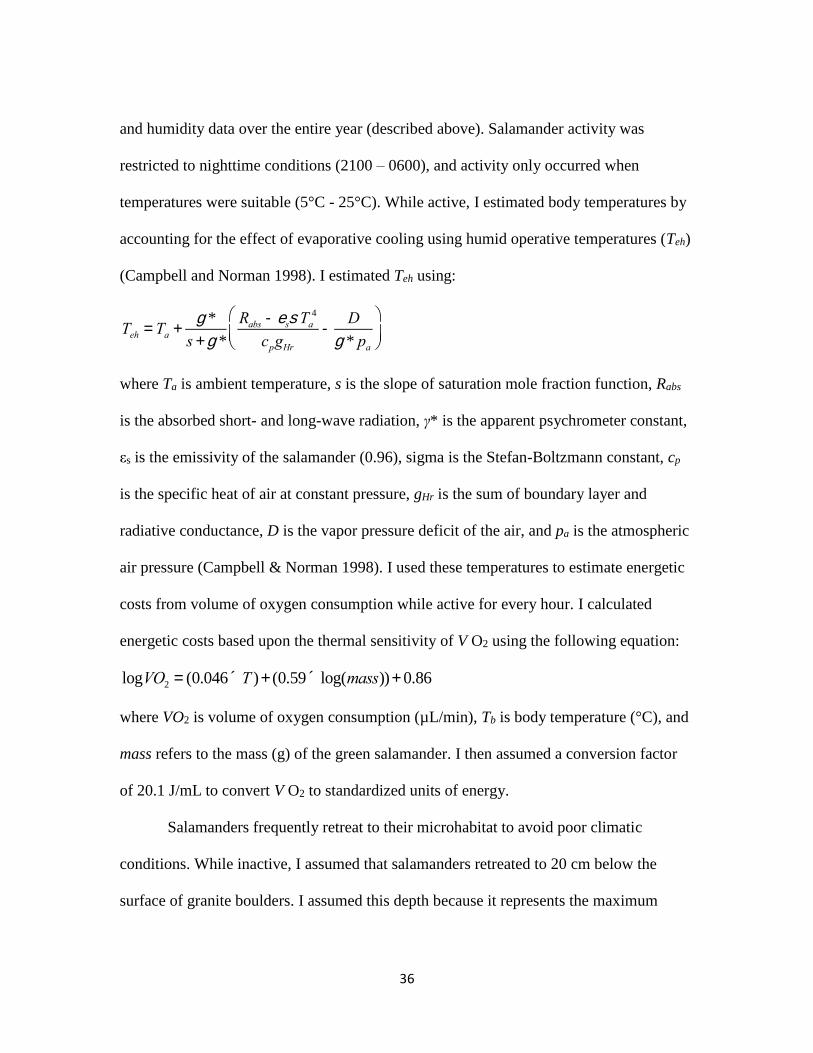
36

and humidity data over the entire year (described above). Salamander activity was

restricted to nighttime conditions (2100 – 0600), and activity only occurred when

temperatures were suitable (5°C - 25°C). While active, I estimated body temperatures by

accounting for the effect of evaporative cooling using humid operative temperatures (Teh)

(Campbell and Norman 1998). I estimated Teh using:

where Ta is ambient temperature, s is the slope of saturation mole fraction function, Rabs

is the absorbed short- and long-wave radiation, γ* is the apparent psychrometer constant,

εs is the emissivity of the salamander (0.96), sigma is the Stefan-Boltzmann constant, cp

is the specific heat of air at constant pressure, gHr is the sum of boundary layer and

radiative conductance, D is the vapor pressure deficit of the air, and pa is the atmospheric

air pressure (Campbell & Norman 1998). I used these temperatures to estimate energetic

costs from volume of oxygen consumption while active for every hour. I calculated

energetic costs based upon the thermal sensitivity of V O2 using the following equation:

where VO2 is volume of oxygen consumption (µL/min), Tb is body temperature (°C), and

mass refers to the mass (g) of the green salamander. I then assumed a conversion factor

of 20.1 J/mL to convert V O2 to standardized units of energy.

Salamanders frequently retreat to their microhabitat to avoid poor climatic

conditions. While inactive, I assumed that salamanders retreated to 20 cm below the

surface of granite boulders. I assumed this depth because it represents the maximum

Teh = Ta +g *

s +g *

Rabs - e ssTa4

cpgHr-

D

g * pa

æ

èç

ö

ø÷

logVO2 = (0.046 ´T )+ (0.59 ´ log(mass))+ 0.86

37

depth at which temperatures approached average temperatures for a given month. I

estimated damping depths based upon the typical properties of granite (Cho, Kwon, and

Choi 2009). I then used the damping depth to determine the temperatures that

salamanders experience during inactivity inside a granite boulder throughout the day. I

assumed that salamanders were not able to forage during times of inactivity. Salamanders

ceased activity upon reaching their dehydration threshold, experiencing temperatures

beyond their preferred range, or during the daytime. I selected a range of dehydration

thresholds (3.5%, 7%, and 10%) at which salamanders ceased activity based upon

empirically-observed values for plethodontids (Feder and Londos 1984). Simulations

were run in an iterative process with each dehydration threshold. I also ran simulations

across various body sizes reflected in our physiological experiments (2 g, 3 g, 4 g) ,

humidity scenarios (+25% and -25% value of VPD), and skin resistance to water loss

(average ri = 7.8 and maximum ri = 14.0) to determine the sensitivity of our predictions

to input parameters. I ran our simulations for every possible combination of body size,

dehydration threshold, humidity scenario, and skin resistance to water loss to estimate

activity budgets and energy balance throughout the year. These physiologically-derived

layers were averaged together to integrate into the correlative framework.

Correlative Species Distribution Model

I used MaxEnt to assess correlations between climatic factors and presence data

because it is known to perform as well or better than other tools during a comprehensive

model evaluation (Elith et al. 2006). It is commonly used to generate distribution models

38

of climate vulnerability (Pearson et al. 2007; Loarie et al. 2008; Puschendorf et at. 2009;

Bradley et al. 2010). I focused on the disjunct population of green salamanders (North

Carolina, South Carolina, and Eastern Georgia). Recent genetic studies have revealed that

this disjunct population, not including the Hickory Nut Gorge region of North Carolina,

is an evolutionary significant unit from the mainland population (J. J. Apodaca, personal

communication). To create the spatial boundaries of our model, I used minimum

bounding geometry in ArcGIS based on known locality points for the species. I created a

25-km buffer around this disjunct range. I extrapolated data on green salamander

movement and predicted that green salamanders could potentially to disperse ~15-km in

33 years if projecting to 2050 (Gordon 1952; Canterbury 1991; see Appendix A). The

remaining 10-km accounts for of the possibility that the current range extends beyond

currently cataloged localities.

I collected green salamander presence data from the South Carolina Department

of Natural Resources, Georgia Department of Natural Resources, North Carolina Wildlife

Resources Commission and publically-accessible online databases (Price and Dorcas

2007; Cicero et al. 2010; USGS 2013). I also gathered new sites in South Carolina from a

recent extensive habitat association survey (Chapter 1). All points were uploaded into

ArcMap 10.3. I reduced clusters of points (and thus removing potential sampling biases

such as repeated sampling from easily-accessible sites) by using a random point generator

in ArcMap. Because the average north-south distance of rock outcrop of sites in South

Carolina was 31-m (Chapter 1), I randomly removed points in clusters that were less than

31m apart.

39

I selected seven bioclimatic variables (BIO 1-2, 4, 8-9, 12, 15; Table 2.1), from a list

of 19 (Hijmans et al. 2005) based on low pairwise correlations between variables.

Although there is a high pairwise correlation value between variables BIO1 and BIO15

(0.74), I wanted to capture two dimensions of precipitation in the analysis. This approach

was first used by Rissler and Apodaca (2007) for west coast congener species, Aneides

falvipunctatus and used has since been used several times to generate distribution models

for amphibians (Milanovich et al. 2010; Barrett et al 2014; Sutton et al 2015). WorldClim

derives these bioclimatic variables from a 30 year (1960-1990) dataset of monthly

averages compiled of temperature and rainfall data at a spatial resolution of ~1km2

(Hijmans et al. 2005). I intersected these climatic variables with both green salamander

presence points and background points in ArcMap (ArcGIS 10.3.1, ESRI). I generated

background points by randomly placing ~2,000 herpetofaunal presence points (Plethodon

yonhalosse, Plethodon teyahalee, Plethodon metcalfi, Plethodon jordani, Terrapene

carolina, Chrysemy picta, Pantherophis obsoletus, Diadophis punctatus, and Storeria

dekayi) collectively distributed through the entire buffered disjunct range of the green

salamander.

I used two different Global Climate Models (GCM), with one Representative

Concentration Pathway (RCP) each. I downloaded two widely used GCM’s from

WorldClim: HadGEM2-CC (Hadley) and CCSM4 (CCSM). Model selection was based

on hindcast accuracy in the northern hemisphere (Overland et al. 2011) and availability of

projected data of the 8.5 RCP. I included two GCMs as the Hadley GCM tends to predict

wetter future species distribution models while the CCSM4 GCM tends to predict dryer

40

future species distribution models (CIESIN 2000). I included the 8.5 RCP trajectory to

provide a perspective representing rapid increase in greenhouse gas emission. MaxEnt

produces species distribution models with climatic suitability (ranging from 0-1

representing low to high habitat suitability). I used two thresholds (strict and moderate) to

generate distributional range shifts in projected suitable habitat within the disjunct range

of green salamanders. I used the fixed cumulative value 10 (F10; a threshold resulting in

10% omission of training data), and the equal training sensitivity plus specificity (ETSP;

threshold that balances the probability of missing suitable sites with the probability of

assigning suitability to a site where the species is absent).

Integration of mechanistic and correlation models

I created a suite of climatic niche models for green salamanders under current and

future climatic conditions. Both correlative and mechanistic data were used within an

inductive, presence-only modeling approach MaxEnt (Phillips et al. 2006). Correlative-

only models were built using only climatic variables, whereas our correlative +

mechanistic models contained climatic variables and two experimentally-derived

mechanistic layers: activity and energetic costs. I compared model predictions using a

variety of methods. Firstly, I compared the number of cells containing suitable habitat

that were lost or gained after mechanism was added to the correlative model. I then

conducted a correlation analysis to see if environmental variables correlated with

differences in predictive ability between model types. Lastly, I tested the null hypothesis

that resistance to water loss was not different among temperature treatments using an

41

analysis of covariance (ANCOVA). To test the assumption of normality I used a Shapiro

Wilk test and QQ plot. I found that one category of the data was significantly not

normally distributed, however, after attempting multiple transformations on the data, I

could not meet this assumption of normality but still proceeded with the analysis. I also

evaluated the significance of the interaction between body mass and temperature on

resistance to water loss, as an ANCOVA assumes an absence of such interaction. The

interaction term was not statistically significant (p=0.29). I tested the differences between

groups by using a Tukey test. I also evaluated the effect of the four temperature

treatments on volume of oxygen consumption (µL/min) using linear regression.

RESULTS

The ANCOVA suggested that both temperature and body mass were significant

(Table 2.2). At the highest temperature treatment (24°C), green salamanders increased

their skin resistance to water loss, ir (Fig 2.2). The results of the Tukey test demonstrated

that the highest treatment was significantly different than the lower two treatments. There

was no significant difference in ir between the lower temperature treatments, 12°C and

18°C (Fig 2.2). Metabolic rates, illustrated by volume of oxygen consumption, increased

with temperature treatments (p < 0.0001, Table 2.3, Fig 2.3). There was a small, but

significant interaction between salamander mass and temperature (p = 0.02; Table 2.3),

such that larger animals increased oxygen consumption at higher temperature more than

smaller animals.

42

I developed 12 species distribution models for green salamanders in their disjunct

range (Fig 2.4). The Hadley GCM models predicted the most suitable habitat followed by

CCSM4 GCM models, and current models (Table 2.4). When mechanism was added to

the current correlative model, there is virtually no change in the number of cells with

suitable habitat (Table 2.4). On the other hand, mechanism reduces 79.9% of cells

containing suitable habitat in the CCSM4 model and 44.7% of cells containing suitable

habitat in the Hadley model (Table 2.4). Among all model runs, the F10 threshold

predicted 1.94 ± 0.67 times more suitable habitat than the ETSP model.

For the three correlative only models, BIO4, BIO15 and BIO12 accounted for 43.6%,

22.2%, and 22.2% of the variation, respectively. For the three correlative + mechanistic

models, BIO4, BIO15 and BIO12 accounted for 41.4%, 22.4%, and 20.4% of the

variation, respectively. None of the environmental variables I evaluated (bioclimatic and

elevation) correlated with the difference values between correlative + mechanistic and

correlative-only models (with correlation values ranging from -0.15 to 0.15). That is, I

were unable to identify any environmental conditions that would predict where one

model type would differ from the other.

DISCUSSION

There have been multiple approaches described in the literature for forecasting

climate change vulnerability, including correlative models and mechanistic models

(Milanovich et al. 2010; Kearney et al. 2010; Barrett et al. 2014; Briscoe et al. 2016;

Mathewson et al. 2017). Such models can be used to construct species distribution

43

models in order to predict climatically suitable habitat for potentially vulnerable species.

Correlative models can be built for a variety of taxa because minimal amounts of data are

required, however, they have a number of untested assumptions. For example, correlative

models exclude mechanism so they do not account for an organism’s biology or

physiology. Also, correlative models are heavily reliant on the quality and spatial

resolution of the environmental data (i.e. GCMs, RCPs) used, so it may be beneficial to

evaluate multiple measures of habitat and used multiple scenarios for future forecasts.

With the incorporation of animal performance, mechanistic models have been shown to

change species distribution models, however, they can also be data intensive (Briscoe et

al. 2016; Mathewson et al. 2017; Riddell et al. 2017). Our study evaluated the effect of

incorporating mechanistic layers into a correlative species distribution model framework.

Our results suggest that under current climatic conditions, correlative models and

correlative + mechanistic models projected nearly congruent suitable habitat for green

salamanders, while under future climatic conditions mechanism reduced suitable habitat

for green salamanders (Table 2.4). Range-wide correlative models show some resiliency

in parts of the disjunct range of the green salamander (Barrett et al. 2014); however, the

addition of physiology in our species distribution models picked up on limitations of the

species not captured by a correlative-only model. Nevertheless, in all model runs some

suitable habitat is projected to remain for the species in 2050. Mechanistic models do not

necessarily yield more restrictive forecasts for species when compared to current climatic

conditions. Green salamanders may present an interesting case because of their

association with rock outcrops, a behavior not shared with congener plethodontids

44

(Gordon 1952; Jaeger 1971; Mount 1975). Green salamanders may have interspecific

aggregation adaptations within rock outcrops allowing them to be more resistant to harsh

conditions (Cupp Jr. 2017), and additionally, keeping them from dispersing long

distances. In other words, green salamanders may be able to tolerate the warmer and

dryer temperatures of granite and may not need to disperse as much as other salamanders

reliant on moist soil (Jaeger 1971).

The laboratory experiments demonstrated that green salamanders increase their skin

resistance to water loss when exposed to higher temperatures. These finding may shed

some light on Gordon’s (1952) preliminary laboratory study, showing green salamanders

were tolerant to warm and dry conditions. Green salamander metabolism increased with

temperature which is consistent with data from other ectotherms (Bartholomew & Tucker

1963; Johnston & Dunn 1987).

In all models, the most variation was explained by BIO4 (temperature

seasonality), BIO15 (precipitation seasonality), and BIO12 (annual precipitation). These

results suggest that environmental seasonality and precipitation play a major role in green

salamander distribution. Green salamanders have well-documented annual cycles,

categorized into four stages: the breeding period (late May to late September), dispersal

and aggregation (late September to November), hibernation (November to late April),

and post-hibernation aggression and dispersal (late April to late May) (Gordon 1952).

Because of these stages, it is likely that green salamanders have different seasonal

requirements for environmental variables. Further, green salamanders are known to use

and breed in moist rock crevices (Gordon 1952), and moisture appears to be a limiting

45

factor in the distribution of other Aneides species (Rosenthal 1957; Spickler et al. 2006;

Haan et al. 2007). Interestingly, both the CCSM4 and the Hadley GCMs appear to be

predicting a wetter future within the BRE (Table 2.5). These wetter projections may

explain why I saw habitat gains in the future models when compared to current models.

Additionally, correlative models may have done a poor job projecting outside of their

range as it is likely that some values for the bioclimatic variables in the 2050 maps were

not present in the current maps. In some cases, there were cells in the 2050 models with

climatic values > 2 standard errors from the mean of the current values.

Knowing when to use a particular distribution modeling can contribute to cost

effective conservation. Under current climate conditions, several studies for endotherms

have demonstrated that correlative models can accurately predict a species distribution

and show minimal changes when mechanistic layers were incorporated (Kearney et al.

2010; Briscoe et al. 2016; Mathewson et al. 2017). Our study provides further evidence

that this approach is likely true for ectotherms as well (Buckley et al. 2010). Collectively,

these studies suggest correlative-only models are probably sufficient for many species

under current climate conditions. Justification for a correlative-only approach is valuable

given the data-intensive nature of mechanistic models. On the other hand, there is

evidence suggesting that mechanism may be important for future projections of species

distributions models. Several studies have shown that mechanism-based forecasts diverge

from those made when using correlative-based models (Briscoe et al. 2016; Mathewson

et al. 2017). Our correlative + mechanistic model supports this trend and thus, I

encourage the use of mechanism (whether physiology, behavior, etc.) in species

46

distribution models for projections assessing climate change vulnerability if resources are

available. With that said, it is unclear whether or not mechanistic models are more

accurate and so there may be an argument to use a more conservative (i.e. restrictive)

threshold. Lastly, our models specifically looked at climatically suitable data only. In

order to make management decisions about where to conserve green salamander habitat,

it would be beneficial to incorporate landscape data (i.e. rocky outcrops, elevation) to

make the most informed decisions.

I used a different approach to creating mechanistic models than others in the

literature who have used Niche Mapper to create their models (Kolbe et al 2010; Briscoe

et al. 2016; Mathewson et al. 2017). Niche Mapper is a program created specifically for

mechanistic models, however, its final output models forecast fundamental niches of the

animals because mechanistic models are independent of presence data (Kearney and

Porter 2004; Porter and Mitchell 2006; Kolbe et al. 2010). The future forecasted

correlative + mechanistic models I created with program MaxEnt diverged from purely

correlative models which has been commonly found in other studies (Buckley et al. 2010;

Kearney et al. 2010; Briscoe et al. 2016; Mathewson et al. 2017). MaxEnt forecasts

models within a correlative framework and thus the output forecasts the realized niche of

an animal (Kearney 2006; Kolbe et al. 2010). Here I suggest an alternative approach to

mechanistic model-making that may narrow down an animal’s fundamental niche to a

realized niche. This approach could potentially solve problems with both mechanistic

models (i.e. honing in on biotic processes that drive species presence) and correlative

47

models (i.e. incorporating organismal performance, estimating outside of the training

data).

When Green Salamander physiology was incorporated into climatic suitability

models, future forecasts predict that suitable habitat for Green Salamanders will be

greatly reduced. According to the strict threshold models, the global circulation models

are predicting much of the suitable habitat for Green Salamanders to be on both National

Forest and state park land in 2050. However, some of the land predicted to be suitable for

Green Salamanders is outside of the protection of public land. Land acquisition in areas

predicted to have suitable Green Salamander habitat (but are outside of public lands) will

help conserve this species for years to come. Periodic monitoring of occupied sites that

fall outside of long-term forecasts of suitability may offer an early-warning signal related

to climate vulnerability.

48

REFERENCES

Araújo MB, Thuiller W, and Pearson RG. 2006. Climate warming and the decline of

amphibians and reptiles in Europe. Journal of Biogeography 33: 1712-1728.

Baillie JEM, Hilton-Taylor C, Stuart SN, editors. 2004. 2004 IUCN Red List of

Threatened Species. A Global Species Assessment. IUCN, Gland, Switzerland

and Cambridge, UK. xxiv + 191 pp.

Barbraud C, Weimerskirch H. 2006. Antarctic birds breed later in response to climate

change. Proceedings of the National Academy of Sciences (USA) 103:6248–

6251.

Barrett K, Nibbelink NP, Maerz JC. 2014. Identifying priority species and conservation

opportunities under future climate scenarios: Amphibians in a biodiversity

hotspot. Journal of Fish and Wildlife Management 5:282-297.

Bartholomew GA, Tucker VA. 1963. Control of changes in body temperature,

metabolism, and circulation by the agamid lizard, Amphibolurus barbatus.

Physiological Zoology xxxvi: 199-218.

Both C, Bouwhuis S, Lessells CM, Visser ME. 2006. Climate change and population

declines in a long-distance migratory bird. Nature 441:81–83.

Bradley B, Wilcove D, Oppenheimer M. 2010. Climate change increases risk of plant

invasion in the Eastern United States. Biological Invasions 12: 1855–1872.

Briscoe NJ, Kearney MR, Taylor C, Wintle BA. 2016. Unpacking the mechanisms

captured by a correlative SDM to improve predictions of climate refugia. Global

Change Biology 22: 2425–2439.

49

Brown JL, Li S, Bhagabati N. 1999. Long-term trend toward earlier breeding in an

American bird: A response to global warming? Proceedings of the National

Academy of Sciences (USA), 96: 5565-5569.

Buckley LB, Urban MC, Angilletta MJ, Crozier LG, Rissler LJ, and Sears MW. 2010.

Can mechanism inform species’ distribution models? Ecology Letters 13:1041–

1054.

Buckley LB. 2008. Linking traits to energetics and population dynamics to predict lizard

ranges in changing environments. American Naturalist 171:E1–E19.

Butchart SHM, et al. 2010. Global biodiversity: Indicators of recent declines. Science

328: 1164-68.

Campbell GS, Norman JM. 1998. An introduction to environmental biophysics. Springer.

Canterbury RA. 1991. Ecology of the Green Salamander, Aneides aeneus (Cope and

Packard), in West Virginia. Master’s Thesis, Marshall University, Huntington,

WV.

Carpenter KE, et al. 2008. One-third of reef-building corals face elevated extinction risk

from climate change and local impacts. Science 321: 560-563.

Cho WJ, Kwon S, Choi JW. 2009. The thermal conductivity for granite with various

water contents. Engineering Geology 107: 167-171.

Cicero C, et al. 2010. VertNet: an online reference Available at:

http://www.vertnet.org/index.html. Accessed March 2017.

CIESIN. 2000. Center for International Earth Science Information Network Climate

Models.http://metroeast_climate.ciesin.columbia.edu/climodels.html Accessed

50

June 2017.

Cope ED, Packard AS. 1881. The fauna of the Nickajack Cave. American Naturalist

15:877–882.

Corser JD. 2001. Decline of disjunct green salamander (Aneides aeneus) populations in

the southern Appalachians. Biological Conservation 97:119–126.

Cupp Jr. PV. 2017. Aneides aeneus (Green Salamander) interspecific aggression.

Herpetological Review 48: 153.

Elith J, Kearney M, Phillips S. 2010. The art of modelling range-shifting species.

Methods in Ecology and Evolution 1: 330-342.

Elith J, et al. 2006. Novel methods improve prediction of species’ distributions from

occurrence data. Ecography 29:129–151.

Füssel HM, Klein RJT. 2006. Climate change vulnerability assessments: an evolution of

conceptual thinking. Climatic Change 75: 301–329.

Gordon RE. 1952. A contribution to the life history and ecology of the plethodontid

salamander Aneides aeneus (Cope and Packard). The American Midland

Naturalist 47: 666-701.

Haan SS, Desmond MJ, Gould WR, Ward Jr JP. 2007. Influence of habitat characteristics

on detected site occupancy of the New Mexico endemic Sacramento Mountains

salamander, Aneides hardii. Journal of Herpetology 41: 1-8.

Hardman RH. 2014. Modeling occurrence of the green salamander, Aneides aeneus, in

the Blue Ridge Escarpment. Master’s Thesis. Western Carolina University,

Cullowhee, NC.

51

Hijmans RJ, Cameron SE, Parra JL, Jones PG, Jarvis A. 2005. Very high resolution

interpolated climate surfaces for global land areas. International Journal of

Climatology 25: 1965–1978.

Jaeger RG. 1971. Moisture as a factor influencing the distributions of two species of

terrestrial salamanders. Oecologia 6: 191-207

Johnston IA, Dunn J. 1987. Temperature acclimation in ectotherms with particular

reference to teleost fish. Symposia of the Society for Experimental Biology 41:

67-93.

Kearney MR, Wintle BA, Porter WP. 2010. Correlative and mechanistic models of

species distribution provide congruent forecasts under climate change.

Conservation Letters 3: 203-213.

Kearney M, Porter WP. 2004. Mapping the fundamental niche: physiology, climate,

and the distribution of a nocturnal lizard. Ecology 85: 3119–3131.

Kearney M. 2006. Habitat, environment, and niche: what are we modeling? Oikos 115:

186-191.

Kolbe JJ, Kearney M, Shine R. 2010. Modeling the consequences of thermal trait

variation for the cane toad invasion of Australia. Ecological Applications

20:2273–2285.

Kusano T, Inoue M. 2008. Long-term trends toward earlier breeding of Japanese

amphibians. Journal of Herpetology 42: 608-614.

Lipps Jr. GJ 2005. A framework for predicting the occurrence of rare amphibians: a case

study with the green salamander. Master’s Thesis. Bowling Green State

52

University, Bowling Green, OH.

Loarie SR, Carter BE, Hayhoe K, McMahon S, Moe R, Knight CA, Ackerley DD. 2008:

Climate change and the future of California’s endemic flora. PLoS ONE 3: e2502.

Mathewson PD, Moyer-Horner L, Beever EA, Briscoe NJ, Kearney M, Yahn JM, Porter

WP. 2017. Mechanistic variables can enhance predictive models of endotherm

distributions: the American pika under current, past, and future climates. Global

Change Biology 23: 1048-1064.

Milanovich JR, Peterman WE, Nibbelink NP, Maerz JC. 2010. Projected loss of a

salamander diversity hotspot as a consequence of projected global climate

change. PLoS ONE 5: e12189.

Mount RH. 1975. The Reptiles and Amphibians of Alabama. Alabama, United States of

America.

Overland JE, Wang M, Bond NA, Walsh JE, Kattsov VM, Chapman WL. 2011.

Considerations in the selection of global climate models for regional climate

projections: The Arctic as a case study. Journal of Climate 24: 1583–1597.

Pearson RG, Raxworthy CJ, Nakamura M, Townsend Peterson A. 2007. Predicting

species distributions from small numbers of occurrence records: a test case using

cryptic geckos in Madagascar. Journal of Biogeography 34: 102–117.

Phillips SJ, Anderson RP, Schapire RE. 2006. Maximum entropy modeling of species

geographic distributions. Ecological Modeling 190: 231-259.

Porter WP, Mitchell JW. 2006. Method and system for calculating the spatial-temporal

effects of climate and other environmental conditions on animals.

53

https://www.google.com/patents/US7155377

Price SJ, Dorcas ME. 2007. Carolina Herp Atlas https://www.carolinaherpatlas.org/.

Accessed March 2017.

Puschendorf R, Carnaval AC, VanDerWal J, Zumbado-Ulate H, Chaves G, Bolaños F,

Alford RA. 2009. Distribution models for the amphibian chytrid Batrachochytrium

dendrobatidis in Costa Rica: proposing climatic refuges as a conservation tool.

Diversity and Distributions. 15: 401-408.

Riddell EA, Apanovitch E, Odum J, Sears MW. 2017. Physical calculations of resistance

to water loss improve predictions of species range models. Ecological

Monographs 87: 21-33.

Riddell EA, Sears MW. 2015. Geographic variation of resistance to water loss within two

species of lungless salamanders: implications for activity. Ecosphere 6: art 86.

Rissler LJ, Apodaca JJ. 2007. Adding more ecology into species delimitation: Ecological

niche models and phylogeography help define cryptic species in the black

salamander (Aneides flavipunctatus). Systematic Biology 56: 924–942.

Roach NS, Hunter EA, Nibbelink NP, Barrett K. 2017. Poor transferability of a

distribution model for a widespread coastal marsh bird in the southeastern United

States. Ecosphere 8:e01715.

Rosenthal GM. 1957 The role of moisture and temperature in the local distribution of the

plethodontid salamander Aneides lugubris. University California Publications in

Zoology 54: 371-420.

Snyder DH. 1983. The apparent crash and possible extinction of the green salamander,

54

Aneides aeneus, in the Carolinas. Association of Southeastern Biologists Bulletin

30:82.

Spickler JC, Sillett SC, Marks SB, Welsh Jr. HH. 2006. Evidence of a new niche for a

North American salamander: Aneides vagrans residing in the canopy of old-

growth redwood forest. Herpetological Conservation and Biology 1: 16-26.

Sutton WB, Barrett K, Moody AT, Loftin CS, deMaynadier PG, Nanjappa P. 2015.

Predicted changes in climatic niche and climate refugia of conservation priority

salamander species in the northeastern United States. Forests 6: 1–26.

Urban MC. et al. 2016. Improving the forecast for biodiversity under climate

change. Science 353: pii: aad8466.

USGS. 2013. Biodiversity Information Serving Our Nation (BISON)

https://bison.usgs.gov/#home. Accessed on March 2017.

Whitford WG, Hutchison VH. 1967. Body size and metabolic rate in salamanders.

Physiological Zoology 40:127–133.

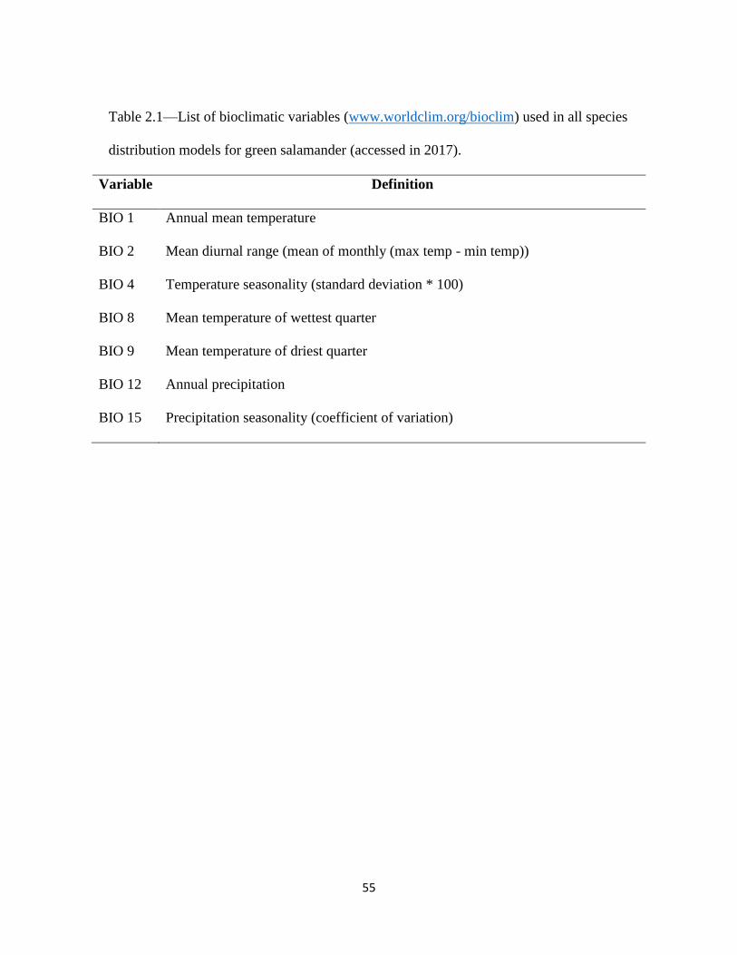
55

Table 2.1—List of bioclimatic variables (www.worldclim.org/bioclim) used in all species

distribution models for green salamander (accessed in 2017).

Variable Definition

BIO 1 Annual mean temperature

BIO 2 Mean diurnal range (mean of monthly (max temp - min temp))

BIO 4 Temperature seasonality (standard deviation * 100)

BIO 8 Mean temperature of wettest quarter

BIO 9 Mean temperature of driest quarter

BIO 12 Annual precipitation

BIO 15 Precipitation seasonality (coefficient of variation)

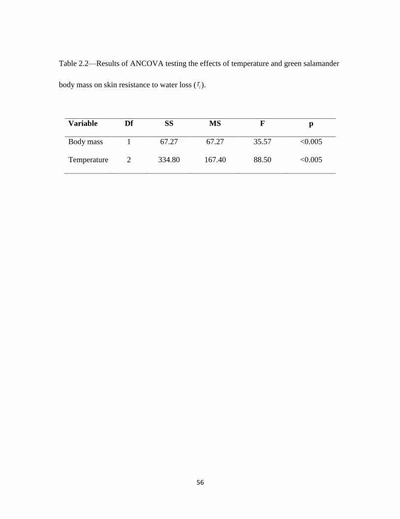
56

Table 2.2—Results of ANCOVA testing the effects of temperature and green salamander

body mass on skin resistance to water loss ( ir ).

Variable Df SS MS F p

Body mass 1 67.27 67.27 35.57 <0.005

Temperature 2 334.80 167.40 88.50 <0.005

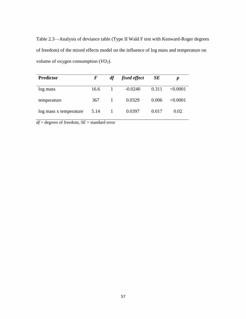
57

Table 2.3—Analysis of deviance table (Type II Wald F test with Kenward-Roger degrees

of freedom) of the mixed effects model on the influence of log mass and temperature on

volume of oxygen consumption (VO2).

Predictor F df fixed effect SE p

log mass 16.6 1 -0.0240 0.311 <0.0001

temperature 367 1 0.0329 0.006 <0.0001

log mass x temperature 5.14 1 0.0397 0.017 0.02

df = degrees of freedom, SE = standard error

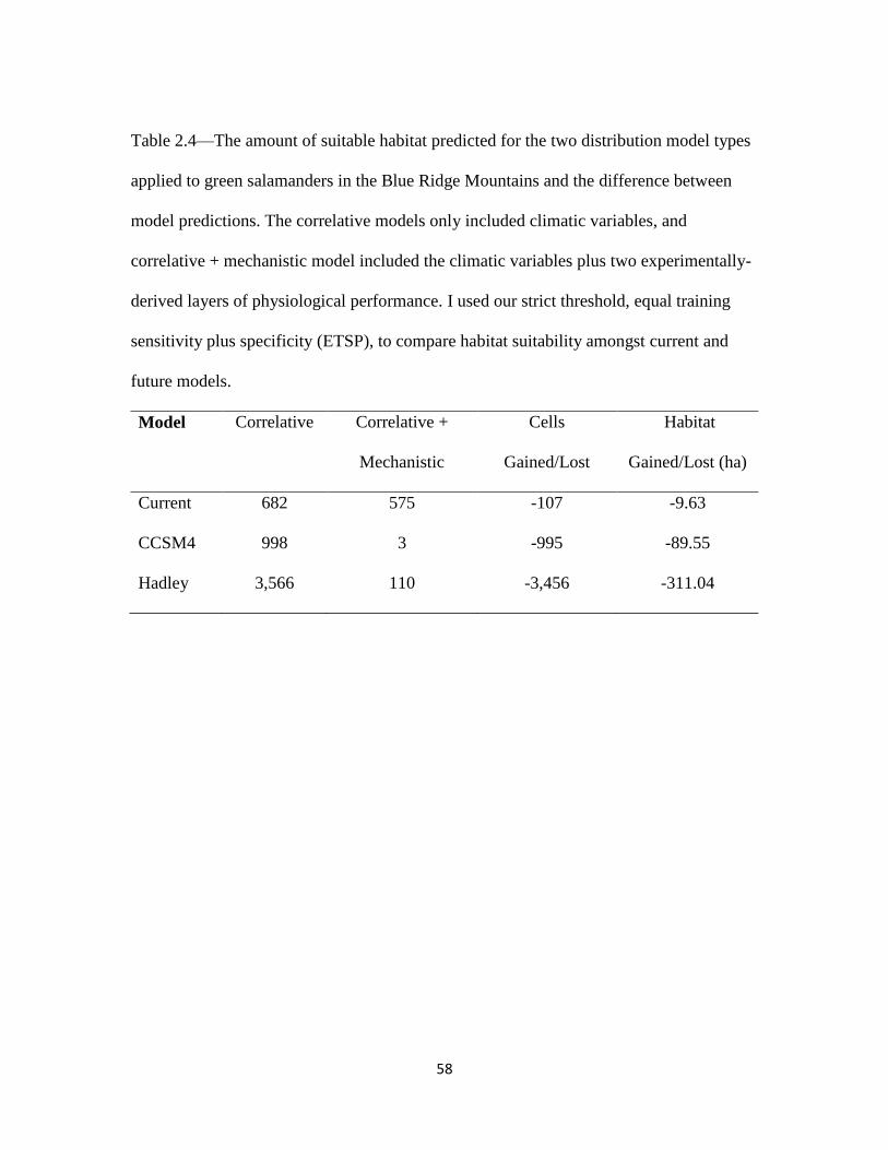
58

Table 2.4—The amount of suitable habitat predicted for the two distribution model types

applied to green salamanders in the Blue Ridge Mountains and the difference between

model predictions. The correlative models only included climatic variables, and

correlative + mechanistic model included the climatic variables plus two experimentally-

derived layers of physiological performance. I used our strict threshold, equal training

sensitivity plus specificity (ETSP), to compare habitat suitability amongst current and

future models.

Model Correlative Correlative +

Mechanistic

Cells

Gained/Lost

Habitat

Gained/Lost (ha)

Current 682 575 -107 -9.63

CCSM4 998 3 -995 -89.55

Hadley 3,566 110 -3,456 -311.04

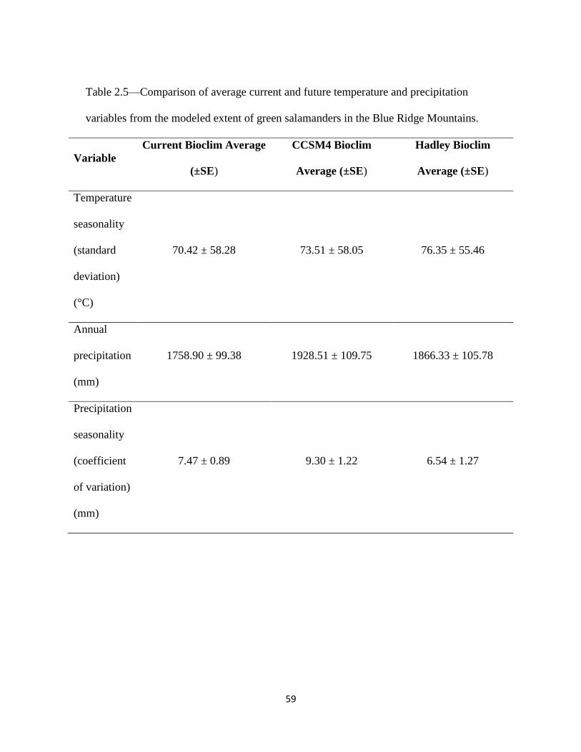
59

Table 2.5—Comparison of average current and future temperature and precipitation

variables from the modeled extent of green salamanders in the Blue Ridge Mountains.

Variable

Current Bioclim Average

(±SE)

CCSM4 Bioclim

Average (±SE)

Hadley Bioclim

Average (±SE)

Temperature

seasonality

(standard

deviation)

(°C)

70.42 ± 58.28

73.51 ± 58.05

76.35 ± 55.46

Annual

precipitation

(mm)

1758.90 ± 99.38

1928.51 ± 109.75

1866.33 ± 105.78

Precipitation

seasonality

(coefficient

of variation)

(mm)

7.47 ± 0.89

9.30 ± 1.22

6.54 ± 1.27

60

FIG 2.1 —Flowchart illustrating the inputs, process, and outputs of mechanistic layers

(activity and energetic costs).

FIG 2.2 —Skin resistance to water loss of green salamanders at three different treatment

temperatures (°C).

FIG 2.3 —Volume of oxygen consumption for green salamanders at four different

treatment temperatures (°C).

Fig 2.4— Projected suitable habitat for green salamanders throughout their disjunct range

for current and 2050 different climatic scenarios. Models predict suitable habitat for

green salamanders under different scenarios by year (current or 2050), global circulation

models (Hadley or CCSM4), one Representative Concentration Pathway (RCP 8.5), and

model threshold (F10 and ETSP). A) The disjunct range of green salamanders located in

North Carolina, South Carolina, and Georgia, USA. B) Species distribution models

categorized by current or future climatic envelopes and then broken down by threshold

61

(moderate or strict). Light blue represents suitable habitat in the correlative only model,

orange represents suitable habitat in the correlative + mechanistic model, dark blue

represents overlapping suitable habitat by the two models (correlative and correlative +

mechanistic), and black represents unsuitable habitat.

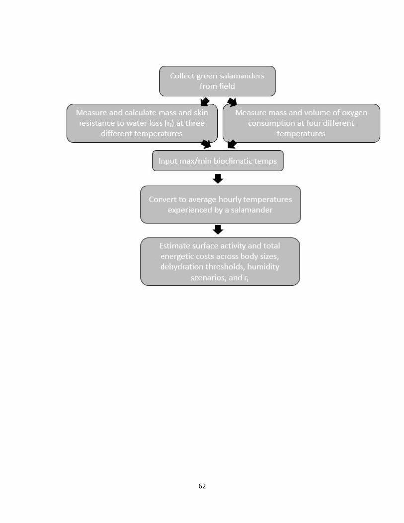
62

63

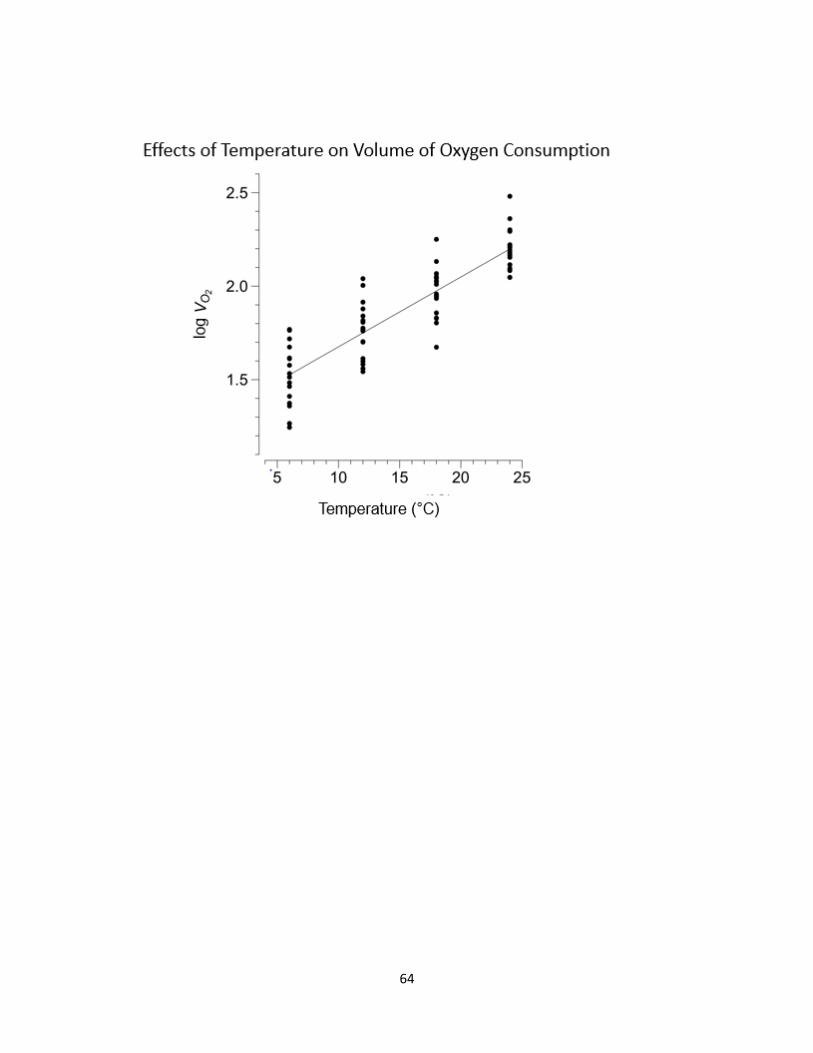
64

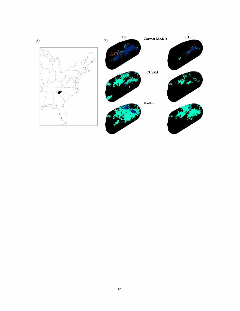
65

66

APPENDICES

67

Appendix A

Estimated Green Salamander Dispersal for the Year 2050

Source Movement

(m) Time(d) Avg_move_day

(m) Avg_move_yr

(m) Avg_move_33yr

(m) Avg_move_33yr

(km)

Gordon 1952 76.2 19 4.010526316 1463.842105 48306.78947 48.30678947

Gordon 1952 76.2 26 2.930769231 1069.730769 35301.11538 35.30111538

Gordon 1952 91.4 91.4 2.995076586 1093.202954 36075.69748 36.07569748

Gordon 1952 0.6 26 0.023076923 8.423076923 277.9615385 0.277961538

Gordon 1952 0.9 273.75 0.003287671 1.2 39.6 0.0396

Gordon 1952 1.8 10 0.18 65.7 2168.1 2.1681

Gordon 1952 0.6 21 0.028571429 10.42857143 344.1428571 0.344142857

Gordon 1952 0.6 18 0.033333333 12.16666667 401.5 0.4015

Gordon 1952 0.6 28 0.021428571 7.821428571 258.1071429 0.258107143

Gordon 1952 3.7 21 0.176190476 64.30952381 2122.214286 2.122214286

Gordon 1952 0.6 1 0.6 219 7227 7.227

Canterbury 1991 25.6 182.5 0.140273973 51.2 1689.6 1.6896

Canterbury 1991 6.4 334.584

0.019128231 6.98180427 230.3995409 0.230399541

Canterbury 1991 7.6 8 0.95 346.75 11442.75 11.44275

Canterbury 1991 46.3 35 1.322857143 482.8428571 15933.81429 15.93381429

Canterbury 1991 46.3 243.334 0.190273451 69.44980973 2291.843721 2.291843721

Canterbury 1991 33.8 60.8334 0.555615829 202.7997778 6692.392666 6.692392666

Canterbury 1991 6.4 14 0.457142857 166.8571429 5506.285714 5.506285714

Canterbury 1991 27.7 14 1.978571429 722.1785714 23831.89286 23.83189286

Canterbury 1991 16.8 4 4.2 1533 50589 50.589

Canterbury 1991 49.4 10 4.94 1803.1 59502.3 59.5023

AVERAGE TOTAL 14.77297652