greenhouse gas emissions from australian beef feedlots
TRANSCRIPT

Greenhouse Gas Emissions from
Australian Beef Feedlots
Stephanie Kate Muir
September 2011
Submitted in total fulfilment of the requirements for the
Degree of Doctor of Philosophy
Department of Agriculture and Food Systems
Melbourne School of Land and Environment
The University of Melbourne
Produced on archival quality paper

i
Abstract
Emissions of the greenhouse gases, methane (CH4) and nitrous oxide (N2O) and the indirect
greenhouse gas ammonia (NH3) play an increasing role in public concern about the
environmental impact of concentrated animal feeding operations, including feedlots.
However, there is a lack of emissions measurements under typical commercial conditions and
there is high uncertainty in the estimation. The lack of accurate measurements and baseline
emissions also makes it difficult to evaluate efficiency of current mangemange practices and
identify the potential reductions under mitigation options. The objective of this study was to
achieve increased understanding of greenhouse gas emissions from Australian beef feedlots,
elucidating the biophysical factors controlling emissions from feedlot systems. Specifically,
the study utilises measurements of greenhouse gas emissions undertaken at commercial
feedlots in Australia using micrometeorological methods and integrates data collected from
the feedlot operators into empirical models with the aim to identify and quantify the sources
of variation in measured emissions between sites and seasons; test the validity the modelling
approach used specifically for feedlots and quantify the link between animal behaviour and
diurnal emissions patterns.
This study comprised two detailed modelling exercises. The first utilising the results of
published studies to validate a range of equations for predicting enteric methane emissions
and for predicting emissions of methane, nitrous oxide and ammonia from manure. The
second modelling exercise utilised the results of measurements undertaken in two commercial
Australian feedlots to evaluate a range of models under commercial conditions. Finally, the
diurnal variation in micrometeorological measurements of CH4 and NH3 were examined in
the context of animal feeding behaviour in order to examine implications for measurement
accuracy and examine correlations between fluxes and behaviour.
This thesis indicates that the current Australian Inventory methodology for estimating
greenhouse gas emissions from feedlots (enteric CH4, manure CH4, N2O and NH3) suffers
from considerable inaccuracies. Although more accurate estimates of CH4 emissions appear to
be associated with utilising an equation based on ration composition, particularly
carbohydrate fractions the current approach over estimates emissions considerably.
Inaccuracies in prediction of emissions of N2O and NH3 are related primarily to the use of
single “emissions factors” which do not adequately reflect the changes in potential emissions

ii
associated with changing environmental conditions.
This thesis also explored the contribution of CH4, N2O and NH3 using IPCC default factor of
1.25% deposited NH3 is lost as N2O to total feedlot emissions, represented as CO2-e. Initial
estimates suggest that feedlot emissions were dominated by CH4, with minor contributions of
direct and indirect N2O. However, based on the measurements nitrogenous greenhouse gases
are predicted to contribute up to 52% of total CO2-e. These results indicate that mitigation
options to reduce feedlot emissions need to be applied to both enteric CH4 and nitrogenous
gas emission, particularly NH3.
These more accurate estimates of greenhouse gas emissions will not only highlight issues
with the current emissions inventory but will also assist the feedlot industry to identify
mitigation strategies to take the benefit from the incentives for reductions in emissions under
the carbon farming initiative (CFI).
iii
Declaration
This is to certify that:
(i) the thesis comprises only my original work towards the PhD except where indicated in the
Preface,
(ii) due acknowledgement has been made in the text to all other material used,
(iii) the thesis is fewer than 100,000 words in length, exclusive of tables, maps, bibliographies
and appendices
Stephanie Muir
29th September 2011

iv
Preface
The whole system feedlot measurements reported in this study were conducted as part of a
larger project (FLOT .331, Greenhouse Gas Emissions from Australian Beef Cattle Feedlots,
Meat and Livestock Australia), reported in Chen et al. (2009).
Measurements were undertaken using open-path lasers (University of Melbourne) and open-
path FTIR (University of Wollongong). Zoe Loh (formally University of Melbourne),
Douglas Rowell (University of Melbourne) and Stephanie Muir were primarily responsible
for the operation of the open-path lasers during the reported field campaigns. The open-path
FTIR was supplied by The University of Wollongong, and operated by Frances Phillips, Mei
Bai and Travis Naylor (University of Wollongong) during the field campaigns. Data analysis
for the emissions measurements using the WindTrax software package was handled primarily
by Douglas Rowell, Frances Phillips and Mei Bai.
Measurements from these field campaigns are reported in Chen et al. (2009) and details about
the open-path FTIR approach were discussed as part of the PhD thesis; Methane Emissions
from Livestock Measured by Novel Spectroscopic Techniques, (Mei Bai, School of
Chemistry, University of Wollongong, June 2010).
The results of these field campaigns are utilised Chapter 5, as a comparison with modelled
results using data collected from the feedlots used in the measurement campaigns and in
Chapter 6, with diurnal emissions profile compared with recorded behaviour. Excluding these
specific measurements, the remainder of the work reported in this thesis was conducted by the
author.
v
Acknowledgements
Whole system measurements of this kind would not have been possible without the whole of
the FLOT.331 project team; Deli Chen, Mei Bai, Tom Denmead, David Griffith, Julian Hill,
Sean McGinn, Travis Naylor, Zoe Loh, Frances Phillips and Doug Rowell. Additional thanks
also to Dr. Sean McGinn and Mr. Trevor Coates (Agriculture and Agri-Food Canada) and
Tom Denmead (CSIRO) for providing expertise and advice in the measurement methodology,
micrometeorology and use of the open-path lasers. Extra thanks to Trevor and Zoe for the
Melbourne to Queensland road trips and to the UOW team for going above physical
chemistry and into the realm of agricultural science when required. Special thanks to Mei for
the dumplings and Travis for excellent BBQ cookery and mid field trip morale boosts.
Thanks also to the owners and managers of the two feedlot sites, for opening their sites to our
team for measurements, providing all the data I asked for and more, allowing video recording
of pens of cattle and access to pens for static chamber measurements.
The FLOT.331 project, which provided the emissions measurement, was funded by Meat and
Livestock Australia and the Australian Government (Australian Greenhouse Office). Meat
and Livestock Australia provided additional funding in the form of a postgraduate top-up
scholarship and operating funds, in conjunction with an Australian Postgraduate Award.
Further financial support for conference attendance was provided by the Farrer Memorial
Trust.
Huge thanks to my supervisory team, Dr. Julian Hill, Professor Deli Chen, Associate
Professor Richard Eckard and Dr. Robert Edis for their support and guidance throughout the
last 4 and a bit years; I’ve learnt a lot from you all. Special thank to Julian for dealing with
numerous panics, general confusion, many phone calls and multiple drafts with good humour
and encouragement. I’m sure it’s been as “good for your soul” as processing pages and pages
of feedlot data into a single number was for mine. Thanks also to Dr. Peter Ades for
biometrical advice during the revisions phase.
Much appreciation goes to my friends, team mates and Dookie campus work mates for
understanding that sometimes I really did just have to stay home and work on my thesis
instead of doing the “much more enjoyable than writing” activity you suggested. Thanks also

vi
for continual encouragement in my quest to be a Doctor of cow “emissions”, even though
exactly what that was and why I wanted to spend all this time working on it probably wasn’t
always clear. Extra special thanks to the fellow PhD candidates among my friends, whether in
the next office or across the country, for all the advice, encouragement and understanding.
Finally, many many thanks to my family, for constantly believing I was nearly finished, even
when I didn’t think so. Dad, I appreciate any and all attempts to “open the gate” for me, not
only in the last few years, but for a lifetime. Mum, thank you for the data entry, but more
importantly for looking after me when I didn’t feel like being a grown up and looking after
myself. Lucy, thank you for your support even though spending so many years studying cows
doesn’t seem normal. I love you all.
Last but not least, thanks to Jack for waggly tail, wet nose and keeping me company while I
was working (e.g. sleeping in front of the fire). Some days a walk is exactly what I need even
when it’s the last thing I think I want.

vii
Table of Contents
Abstract ..................................................................................................................................... i
Declaration .............................................................................................................................. iii
Preface ..................................................................................................................................... iv
Acknowledgements ...................................................................................................................v
Table of Contents................................................................................................................... vii
List of Tables......................................................................................................................... xiv
List of Figures ....................................................................................................................... xix
Abbreviations...................................................................................................................... xxvi
Associated Publications...................................................................................................... xxix
Chapter 1. Introduction ...........................................................................................................1
1.1 Global Demand for Beef ..................................................................................................1
1.2 Feedlot Systems................................................................................................................1
1.3 The Global Emissions Problem........................................................................................2
1.4 Issues for the Feedlot Sector.............................................................................................4
1.5 Feedlot Emissions Balance...............................................................................................4
1.6 Summary ..........................................................................................................................5
1.7 Objectives .........................................................................................................................5
Chapter 2. Literature Review..................................................................................................6
2.1 Introduction ......................................................................................................................6
2.2 Emissions Sources in the Feedlot .....................................................................................6
2.2 Enteric CH4 Emissions Process ........................................................................................7
2.2.1 Enteric CH4 Emissions from Lot Fed Cattle............................................................10
2.2.2 Animal Factors Influencing Enteric CH4 Emissions ...............................................11
2.2.3 Ration Composition Effects.....................................................................................11
2.3 Methane Emissions from Manure...................................................................................13
2.3.1 Methane Emissions Process.....................................................................................13

viii
2.3.2 Emissions Potential .................................................................................................14
2.3.3 Factors Influencing CH4 emissions from Manure ...................................................15
2.4 Nitrogenous Gases..........................................................................................................19
2.5 Nitrous Oxide Emissions Process...................................................................................19
2.5.1 N2O Emissions Potential .........................................................................................20
2.5.2 Factors Influencing Emissions of N2O ....................................................................20
2.6 Ammonia Emissions Process .........................................................................................23
2.6.1 Potential NH3 Emissions from Feedlots ..................................................................24
2.6.2 Factors Influencing NH3 Emissions.........................................................................24
2.7 Quantification of Enteric Emissions...............................................................................28
2.7.1 Calorimetric/ Chamber Methods .............................................................................28
2.7.2 Tracer Techniques ...................................................................................................29
2.8 Quantification of Manure Emissions..............................................................................31
2.8.1 Chamber Approaches ..............................................................................................31
2.9 Whole System Measurements ........................................................................................33
2.10 Modelling Emissions ....................................................................................................35
2.10.1 Enteric CH4............................................................................................................36
2.10.2 Modelling Manure Emissions................................................................................37
2.10.3 Ammonia ...............................................................................................................37
2.10.4 Nitrous Oxide ........................................................................................................38
2.10.5 Manure Methane....................................................................................................39
2.11 Summary ......................................................................................................................40
Chapter 3. General Methodology..........................................................................................42
3.1 Site Selection..................................................................................................................42
3.2 Emissions Measurements ...............................................................................................43
3.2.1 Open-Path Spectroscopy..........................................................................................45
3.2.2 Micrometeorology ...................................................................................................45

ix
3.2.3 Atmospheric Dispersion Modelling.........................................................................45
3.3 Units of Measurement/ Calculations ..............................................................................48
3.4 Statistical Analysis .........................................................................................................48
3.5 Feedlot Data Collection..................................................................................................48
3.6 Emissions Models...........................................................................................................49
3.6.1 Structure ..................................................................................................................49
3.6.2 Data Source .............................................................................................................49
3.6.3 Intake Model............................................................................................................49
3.7 Methane Model...............................................................................................................50
3.7.1 Enteric CH4 Emissions ............................................................................................50
3.7.2 Manure CH4 Emissions ...........................................................................................52
3.8 Nitrogen Model ..............................................................................................................53
3.9 Assumptions ...................................................................................................................55
3.10 Validation .....................................................................................................................56
3.10.1 Enteric CH4 Model ................................................................................................56
3.10.2 Nitrogen Model .....................................................................................................57
3.11 Comparison with Australian Feedlot Measurements....................................................58
3.12 Statistical Analysis .......................................................................................................58
3.13 Animal Behaviour ........................................................................................................59
3.13.1 Pen Selection .........................................................................................................59
3.13.2 Observations ..........................................................................................................59
3.13.3 Animal Details.......................................................................................................60
3.13.4 Statistical Analysis ................................................................................................60
Chapter 4. Evaluation of a Methodology for Estimation of Greenhouse Gas Emissions
from Feedlot Systems .............................................................................................................62
4.1 Introduction ....................................................................................................................62
4.1.1 Inventories and Emissions Reporting ......................................................................62

x
4.1.2 Research Question ...................................................................................................63
4.2 Model Development/Structure .......................................................................................64
4.2.1 IPCC Tier I and Tier II Equations ...........................................................................64
4.2.2 Moe and Tyrell (1979) Equation .............................................................................65
4.2.3 Blaxter and Clapperton (1965) Equation.................................................................67
4.2.4 Ellis et al. (2007) Equation......................................................................................67
4.2.5 Ellis et al. (2009) Equation......................................................................................68
4.2.6 Manure CH4 Estimation...........................................................................................68
4.2.7 Nitrogen Excretion and Emissions ..........................................................................68
4.3 Methods ..........................................................................................................................69
4.3.1 Enteric CH4 Validation............................................................................................69
4.3.2 Nitrogen Transactions..............................................................................................73
4.4 Sensitivity Testing..........................................................................................................78
4.4.1 Intake Prediction......................................................................................................78
4.4.2 Gross Energy Estimation.........................................................................................79
4.5 Results ............................................................................................................................81
4.5.1 Enteric CH4..............................................................................................................81
4.5.2 Nitrogen Transactions..............................................................................................84
4.5.3 Gaseous Nitrogen Emissions...................................................................................88
4.5.4 Sensitivity Testing ...................................................................................................89
4.6 Discussion ......................................................................................................................92
4.6.1 Accuracy of the Models for Feedlot Systems..........................................................92
4.6.2 Sensitivity of Models...............................................................................................98
4.6.3 Further Considerations ............................................................................................99
4.7 Conclusion....................................................................................................................101
Chapter 5. Measured Emissions and Application of a Model for Estimation of
Greenhouse Gas Emissions from Australian Beef Feedlots..............................................103

xi
5.1 Introduction ............................................................................................................103
5.1 Research Questions ..................................................................................................105
5.2 Methodology.............................................................................................................105
5.2.1 Assumptions ..........................................................................................................106
5.2.2 Emissions from Manure.........................................................................................108
5.2.3 Statistical Analysis ................................................................................................109
5.2.4 Input Data ..............................................................................................................109
5.3 Results ..........................................................................................................................120
5.3.1 Accuracy of Prediction ..........................................................................................120
5.3.2 Southern Site .........................................................................................................123
5.3.3 Northern Site .........................................................................................................126
5.3.4 Seasonal Differences .............................................................................................129
5.3.6 Combined Data......................................................................................................130
5.4 Discussion ....................................................................................................................133
5.4.1 Measured Emissions..............................................................................................133
5.4.2 Emissions Prediction .............................................................................................137
5.4.3 Site Specific Differences .......................................................................................139
5.4.4 Season Specific Differences ..................................................................................143
5.4.5 Combined Data Set................................................................................................146
5.4.6 Role of DMI ..........................................................................................................146
5.5 Conclusion....................................................................................................................147
Chapter 6. Correlations between Diurnal Patterns of Greenhouse Gas Emissions and
Feeding Behaviour of Feedlot Cattle ..................................................................................149
6.1 Introduction ..................................................................................................................149
6.1.2 Research Questions ...............................................................................................150
6.2 Materials and Methods: ................................................................................................150
6.2.1 Site Selection .........................................................................................................150

xii
6.2.2. Animal Characteristics .........................................................................................150
6.2.3 Behavioural Observations......................................................................................151
6.2.4 Micrometeorological Measurements .....................................................................152
6.2.5 Environmental Data...............................................................................................152
6.2.6 Statistical Analysis ................................................................................................152
6.3 Results ..........................................................................................................................153
6.3.1 Northern Site- Winter 2007 ...................................................................................153
6.3.2 Southern Site- Winter 2007 ...................................................................................156
6.3.3. Northern Site- Summer 2008................................................................................159
6.3.4 Southern Site- Summer 2008.................................................................................162
6.5 Discussion ....................................................................................................................165
6.5.1 Cattle Behaviour....................................................................................................165
6.5.2 Fluxes ....................................................................................................................166
6.5.3 Correlations ...........................................................................................................166
6.5.4 Other Considerations .............................................................................................167
6.6 Conclusion....................................................................................................................169
Chapter 7. General Discussion ............................................................................................170
7.1. Introduction .................................................................................................................170
7.2 Feedlot Production........................................................................................................170
7.3 The Need for Accounting .............................................................................................171
7.3.1 Measurement as an Accounting Method ...............................................................172
7.3.2 Modelled Emissions Estimates for Accounting.....................................................174
7.4 Implication of Inaccurate Accounting ..........................................................................175
7.5 Opportunities ................................................................................................................176
7.6 Implications ..................................................................................................................178
7.7 Conclusion....................................................................................................................181
Chapter 8. References ..........................................................................................................182

xiii
Chapter 9. Appendices .........................................................................................................206
9.1 Appendix for Chapter 3- Lin’s concordance ................................................................206
9.2 Appendix for Chapter 3- General Model Structure ......................................................207
9.3 Appendix for Chapter 4- Measured and Predicted Emissions......................................208
9.4 Appendix for Chapter 5- Measured and Predicted Emissions......................................211
9.5 Appendix for Chapter 6- Full Diurnal Emissions Patterns...........................................212

xiv
List of Tables
Table 3.1 Dates of sampling period, number of head and proportion of pens occupied
during eight field campaigns at two beef cattle feedlots, Northern (Queensland) and
Southern (Victoria) during Winter 2006, Summer 2007, Winter 2007 and Summer
2008...................................................................................................................................... 44
Table 3.2 Standard intake values for feedlot cattle based on the National Inventory
Methodology for the Estimation of Greenhouse Sources and Sinks (2006)........................ 50
Table 3.3 Assumptions of the standard model.................................................................... 56
Table 4.1 Studies selected for evaluation of the standard model, comparisons of the
model and physiological response tested in the model........................................................ 70
Table 4.2 Ration characteristics of the studies utilised for validation of the enteric CH4
model.................................................................................................................................... 71
Table 4.3 Published animal production data and measured enteric CH4 emissions used
in validation of the model (mean and standard deviation)................................................... 72
Table 4.4 Studies selected for validation of the model for nitrogen transactions in the
animal and primary parameter investigated......................................................................... 73
Table 4.5 Animal production data used in the validation of the model for nitrogen
transactions (mean and standard deviation)......................................................................... 74
Table 4.6 Ration details of the studies used in the validation of the model for nitrogen
transactions........................................................................................................................... 75
Table 4.7 Studies selected for the validation of the model for nitrogen gas, major gas
measured and measurement approach.................................................................................. 76

xv
Table 4.8 Treatments, N intakes and excretion and measured N emissions (N2O and
NH3) used in the validation of the N gas model................................................................... 77
Table 4.9 Fitted Linear relationships between measured and predicted CH4 emissions
based on five equations utilising the results of published studies........................................ 80
Table 4.10 Variation in predicted intake for a number of studies based on a set class
based value, the equation of Minson and McDonald (1987), and a value derived from
percentage live weight.......................................................................................................... 81
Table 4.11 Lin’s concordance correlation coefficients between measured and predicted
emissions of CH4 using 5 equations based on the results of published studies................... 81
Table 4.12 Fitted Linear relationships between measured and predicted values for N
excretion parameters based on published studies................................................................. 84
Table 4.13 Concordance and correlations between measured and predicted values for N
excretion based on published studies................................................................................... 85
Table 4.14 Linear relationships between measured and predicted emissions of
nitrogenous gases based on published studies...................................................................... 88
Table 4.15 Concordance and correlations between measured and predicted emissions of
Nitrogenous gases................................................................................................................ 88
Table 4.16 Concordance and correlations between measured CH4 output and CH4 output
predicted using measured intake, intake as a set value based on cattle class, intake
calculated based on the equation of (Minson and McDonald 1987), and intake as a
percentage of live weight. Predicted CH4 is based on five different equations................... 90
Table 4.17 Reported and calculated* weighted average GE concentrations of rations
used in the validation studies............................................................................................... 91
Table 5.1 Standardised values utilised in the prediction of greenhouse gas emissions
from beef feedlot cattle........................................................................................................ 107

xvi
Table 5.2 Feedlot stock characteristics (mean and SD) averaged over the duration of
eight measurement campaigns. Data was collected from feedlot operators in the form of
standard management software outputs............................................................................... 111
Table 5.3 Environmental conditions at two feedlot sites (northern and southern
Australia) during eight measurement campaigns (covering summer and winter)...............
112
Table 5.4 Means and standard errors of per-head emissions (g/head/day) of CH4, NH3
and N2O during eight field campaigns. Measurements of CH4 and NH3 were made by
three separate instruments (two open-path-lasers and an open-path FTIR) in concert
(combined values shown). N2O measurements were made by open-path FTIR only.......... 113
Table 5.5 Major ration Ingredients and proportions of grain at two feedlots sites over
eight measurement campaigns............................................................................................. 115
Table 5.6 Ration composition and nutritive values required for predicting enteric CH4
(using five equations), manure CH4, NH3 and N2O emissions from feedlot beef cattle...... 117
Table 5.7 Fitted Linear relationships and SE for measured and predicted greenhouse gas
emissions at two feedlot sites over seven measurement campaigns.................................... 120
Table 5.8 Concordance and correlations between measured and predicted greenhouse
gas emissions at two feedlot sites over eight measurement campaigns............................... 121
Table 5.9 Fitted linear relationships and SE for predicted and measured greenhouse gas
emissions from a Southern Australian feedlot site over four measurement
campaigns............................................................................................................................. 124
Table 5.10 Concordance and correlations between predicted and measured greenhouse
gas emissions from a Southern Australian feedlot site over four measurement
campaigns............................................................................................................................. 124

xvii
Table 5.11 Fitted linear relationships and SE for predicted and measured greenhouse gas
emissions from a Northern Australian feedlot site over four measurement
campaigns............................................................................................................................. 127
Table 5.12 Concordance and correlations between measured and predicted greenhouse
gas emissions from a Northern Australian feedlot site over four measurement
campaigns............................................................................................................................. 127
Table 5.13 Fitted linear relationships and SE for measured and predicted emissions of
CH4, N2O and NH3 based on published values and measurements from two Australian
feedlots over seven measurement campaigns. Predicted emission of CH4 is based on
three equations...................................................................................................................... 131
Table 5.14 Concordance and correlations between measured and predicted emissions of
CH4, N2O and NH3 based on published data (as used in the evaluation reported in
Chapter 4) and measurements from two Australian feedlots over seven measurement
campaigns. 131
Table 6.1 Correlation Matrix (and t-probabilities) for animal behaviour and greenhouse
gas fluxes measured at the Northern Site during winter...................................................... 154
Table 6.2 Correlation matrix (and t-probabilities) for animal behaviour and greenhouse
gas fluxes measured at the Southern Site during winter...................................................... 156
Table 6.3 Correlation matrix (and t-probabilities), for animal behaviour and greenhouse
gas fluxes measured at the Northern Site during summer 2008........................................... 159
Table 6.4 Correlation matrix (and t-probabilities), for animal behaviour and greenhouse
gas fluxes measured at the Southern Site during summer.................................................... 162
Table 9.1 Published and modelled CH4 emissions (g/head/day) used in the model
validation.............................................................................................................................. 208
xviii
Table 9.2 Published and predicted values (g/head/day) of nitrogen intake and excretion
used in the validation of the nitrogen model........................................................................ 209
Table 9.3 Published and Predicted emissions (g/head/day) of emissions of NH3 and N2O
used in the validation of the model for N gas...................................................................... 210

xix
List of Figures
Figure 2.1 Emissions sources in a feedlot. This study focuses on the direct emissions from
livestock and emissions from manure……………………………………………………….. 7
Figure 2.2 Stylised representation of three significant factors influencing emissions of
methane from feedlot manure; ration forage and concentrate contents (A), moisture (B) and
temperature (C)………………………………………………………………………………. 17
Figure 2.3 Stylised representations of three key factors controlling N2O. (A) Dietary
nitrogen, (B) water filled pore space (through effect on aeration) and (C) Soil compaction
(through effect on aeration)…………………………………………………………………. 22
Figure 2.4 Stylaised representation of three factors influcencing ammonia volatilisation
from feedlot manure; (A) Dietary Nitrogen, (B) Substrate pH and (C) Environmental
Temperature………………………………………………………………………………….. 27
Figure 3.1 Difference between mean minimum and maximum temperatures and mean
monthly rainfall for the Northern feedlot site, 1992-2009, Bureau of Meteorology Climate
Statistics (Dalby Airport Station). Mean annual maximum temperature; 26.9°C, mean
annual minimum temperature; 12°C, total annual rainfall; 606.2
mm............................................................................................................................................ 42
Figure 3.2 Difference between maximum and minimum monthly temperatures and mean
monthly rainfall for the Southern feedlot site, temperature 1966-2000, rainfall 1966-2009,
Bureau of Meteorology Climate Statistics (Donald Station- Charlton station has been
closed since 1976). Mean annual maximum temperature; 21.3°C, mean annual minimum
temperature; 8.8°C, total annual rainfall; 380.8 mm................................................................ 43
Figure 4.1 Comparison of measured and predicted emissions (from published studies) of
the energetic based models for prediction of enteric CH4 emissions. IPCC Tier I (A), IPCC
Tier II (B) and Blaxter and Clapperton (1965)(C). Horizontal error bars indicate SD of
measured emissions; vertical error bars indicate SD of predicted emissions........................... 82

xx
Figure 4.2 Comparison of measured and predicted emissions (from published studies) of
the CHO based models for prediction of enteric CH4 emissions. Moe and Tyrrell (1979)(A),
Ellis et al. (2007)(B) and Ellis et al. (2009)(C). Horizontal error bars indicate standard
deviation in measured emissions; vertical error bars indicate SD of predicted
emissions...................................................................................................................................
83
Figure 4.3 Comparison between measured and predicted values of N intake (A), N
retention (B) and Excretion of faecal N (C) based on published studies. Horizontal error
bars indicate SD of measured emissions; vertical error bars indicate SD of predicted
emissions.................................................................................................................................. 86
Figure 4.4 Comparison between measured and predicted values of Urinary N excretion
(A), Total N excretion (B) and volatile NH3 (C) based on published studies. Horizontal
error bars indicate SD of measured emissions; vertical error bars indicate SD of predicted
emissions.................................................................................................................................. 87
Figure 5.1 Comparison between measured and predicted emissions of enteric CH4 from
two Australian feedlot sites using three equations; IPCC Tier II (A), Moe and Tyrrell
(1979) (B) and Ellis et al. (2007)(C). Horizontal error bars indicate SD of measured
emissions (averaged over the whole measurement campaign); vertical error bars indicate
SD of predicted emissions (averaged over the whole measurement campaign)…………….. 122
Figure 5.2 Comparison between measured and predicted emission of NH3 (A) and N2O (B)
from two Australian feedlot sites. Horizontal error bars indicate SD of measured emissions
(averaged over the whole measurement campaign); vertical error bars indicate SD of
predicted emissions (averaged over the whole measurement campaign)……………...…….. 123
Figure 5.3 Comparison between measured and predicted emissions of enteric CH4 using
IPCC Tier II (A), (Moe and Tyrrell 1979) (B) and (Ellis et al. 2007) (C) from a southern
Australian feedlot site. Horizontal error bars indicate SD of measured emissions (averaged
over the whole measurement campaign); vertical error bars indicate SD of predicted
emissions (averaged over the whole measurement campaign)................................................. 125

xxi
Figure 5.4 Comparison between measured and predicted emissions of NH3 (A) and N2O
(B) from a southern Australian feedlot site. Horizontal error bars indicate SD of measured
emissions (averaged over the whole measurement campaign); vertical error bars indicate
SD of predicted emissions (averaged over the whole measurement campaign)…................. 126
Figure 5.5 Comparison between measured and predicted emissions of enteric CH4 using
IPCC Tier II (A), Moe and Tyrrell (1979) (B) and Ellis et al. (2007) (C) from a northern
Australian feedlot site. Horizontal error bars indicate SD of measured emissions (averaged
over the whole measurement campaign); vertical error bars indicate SD of predicted
emissions. (averaged over the whole measurement campaign)................................................
128
Figure 5.6 Comparison between measured and predicted emissions of NH3 (A) and N2O
(B) from a northern Australian feedlot site. Horizontal error bars indicate SD of measured
emissions (averaged over the whole measurement campaign); vertical error bars indicate
SD of predicted emissions. (averaged over the whole measurement campaign)..................... 129
Figure 5.7 Comparison between measured and predicted enteric methane emissions based
on a database of published studies, and measurements from two Australian feedlot sites.
Predictions were based on three equations IPCC Tier II (A), Moe and Tyrrell (1979) (B)
and Ellis et al. (2007) (C)......................................................................................................... 132
Figure 5.8 Comparison between measured and predicted emissions of Nitrogenous gases;
NH3 (A) and N2O (B) from a database of published studies and measurements from two
Australian feedlot sites............................................................................................................. 133
Figure 6.1 Emission of CH4 and NH3 (flux rates calculated to g/head/day) and air
temperature (°C). Error bars indicate LSD for significance at P<0.05 level............................ 154
Figure 6.2 Number of cattle feeding and ruminating over 12 hours during winter at the
Northern Site. Error bars indicate LSD for significance at P<0.05 level................................. 155
Figure 6.3 Emission of CH4 and NH3 (flux rates calculated to g/head/day) and air
temperature (C). Error bars indicate standard deviation in flux rate (g/head/day) or
temperature. Error bars indicate LSD for significance at P<0.05 level.................................... 157
Figure 6.4 Number of cattle feeding and ruminating over 12 hours during winter at the
Southern Site. Error bars indicate LSD. for significance at P<0.05 level................................ 158

xxii
Figure 6.5 Emission of CH4 and NH3 (flux rates calculated to g/head/day) and air
temperature (°C). Error bars indicate LSD for significance at P<0.05 level............................ 160
Figure 6.6 Number of cattle feeding and ruminating over 12 hours during summer at the
Northern Site. Error bars indicate LSD for significance at P<0.05 level................................. 161
Figure 6.7 Emission of CH4 and NH3 (flux rates calculated to g/head/day) and air
temperature (C). Error bars indicate LSD for significance at P<0.05 level.............................
163
Figure 6.8 Number of cattle feeding and ruminating over 12 hours during summer at the
Southern Site. Error bars indicate LSD. for significance at P<0.05 level................................
164
Figure 9.1 Calculation of Cb a bias correction factor that measured how far the best-fit line
deviates from the 45° line (measure of accuracy). Reproduced from Lin (1989)…………… 206
Figure 9.2 Calculation of the concordance correlation coefficient. Reproduced from Lin
(1989)………………………………………………………………………………………… 206
Figure 9.3 Diagrammatic representation of the basic modelling approach used to estimate
greenhouse gas emissions from feedlot systems. The principal domains of each equation or
set of equations is indicated by the dotted lines. Transfers of information between parts of
the model are indicated by the arrows...................................................................................... 207
Figure 9.4 15 minute average CH4 (g/head/day) and NH3 (g/head/day) fluxes from the
Northern Site measured during winter 2007............................................................................. 212
Figure 9.5 15 minute average CH4 (g/head/day) and NH3 (g/head/day) fluxes from the
Northern Site measured during summer 2008.......................................................................... 213
Figure 9.6 15 minute average CH4 (g/head/day) and NH3 (g/head/day) fluxes from the
Southern Site measured during winter 2007............................................................................. 214
Figure 9.7 15 minute average CH4 (g/head/day) and NH3 (g/head/day) fluxes from the
Southern Site measured during summer 2008.......................................................................... 215

xxiii
List of Equations
Equation 2.1 Methane production from carbohydrate (Saggar et al. 2004b)..................... 8
Equation 2.2 Reduction of CO2 to form CH4 (O’Mara 2004)............................................ 8
Equation 2.3 Basic CH4 production from fermentation in manure (Saggar et al.
2004b).................................................................................................................................. 19
Equation 2.4 Nitrification (Saggar et al. 2004b)................................................................ 20
Equation 2.5 Denitrification (Saggar et al. 2004b)............................................................ 21
Equation 2.6 The urea hydrolysis reaction produces ammonium from urea (Saggar et al.
2004b).................................................................................................................................. 23
Equation 2.7 Ammonia volatilisation (Saggar et al. 2004b).............................................. 23
Equation 2.8 Hydrolysis of urea in the presence of water, to NH3, at an alkaline pH.
This is a bidirectional process, with formation of urea as pH decreases (Rhoades et al.
2008)………………………………………………………………………………………. 26
Equation 2.9 Determination of CH4 emission rate using SF6............................................ 30
Equation 3.1 Prediction of dry matter intake from the growth and live weight of beef
cattle based on Minson and McDonald (1987).................................................................... 50
Equation 3.2 Enteric CH4 Production; Moe and Tyrell (1979).......................................... 51
Equation 3.3 Enteric CH4 production; Blaxter and Clapperton (1965).............................. 51
Equation 3.4 Enteric CH4 Production; Ellis et al. (2007).................................................. 52
Equation 3.5 Enteric CH4 production; Ellis et al. (2009).................................................. 52
Equation 3.6 Volatile solids excretion............................................................................... 53
Equation 3.7 CH4 production from manure....................................................................... 53
Equation 3.8 Faecal N excretion........................................................................................ 54
Equation 3.9 Nitrogen Retention........................................................................................ 54

xxiv
Equation 3.10 Calculation of Urinary N excretion using a mass balance approach.......... 54
Equation 3.11 Estimated N2O Emissions from faecal N.................................................... 54
Equation 3.12 Nitrous oxide Emitted from urinary N........................................................ 55
Equation 3.13 Loss of volatile NH3 from faecal N............................................................ 55
Equation 3.14 Loss of volatile NH3 from urinary N.......................................................... 55

xxv
List of Plates
Plate 3.1 Tuneable diode laser (left) and micrometeorological equipment (centre) at the
Southern Site........................................................................................................................ 47
Plate 3.2 An example of a WindTrax project screen depicting backward Lagrangian
Stochastic (bLS) modelling of gas flux from a single sensor, during a single 15-minute
period. Gas-flux is estimated as the rate of gas emission (gGAS.m2.s1) from the
contributing source area (the footprint of red touchdowns) that would have resulted in
the measured gas concentration at the sensor given the prevailing wind speed, wind
direction and turbulence measured by the micrometeorological
station.................................................................................................................................. 47
Plate 3.3 Video camera mounted in the Northern (A) and Southern (B) feedlots.............. 61

xxvi
Abbreviations
ABARE- Australian Bureau of Agricultural and Resource Economics
ADF- Acid Detergent Fibre
ADFi- Intake of Acid Detergent Fibre
ADG- Average Daily Gain
AGO- Australian Greenhouse Office
ALFA- Australian Lot Feeders Association
ANOVA- Analysis of Variance
bLS- Backward Lagrangian Stochastic (model)
C- Carbon
CELLi- Intake of Cellulose
CFI- Carbon Farming Initiative
CH4- Methane
CHO- Carbohydrate
CNCPS- Cornel Net Crude Protein System
CO2- Carbon Dioxide
CO2-e- Carbon Dioxide Equivalent
CP- Crude Protein
CPi- Crude Protein Intake
CV- Coefficient of Variation
DCCEE- Department of Climate Change and Energy Efficiency
DM- Dry Matter

xxvii
DMI- Dry Matter Intake
DOF- Days on Feed
EF- Emissions Factor
FATi- intake of Fat
FTIR- Fourier Transfer Infra-Red
GE- Gross Energy
GEI- Gross Energy Intake
GWP- Global Warming Potential
HEMIi- Intake of Hemicellulose
H2- Hydrogen Gas
IPCC- Intergovernmental Panel on Climate Change
KCL Potassium Chloride
LIGi- Intake of Lignin
LSD- Least Significant Difference
LWG- Liveweight gain
LWT- Liveweight
MAF- Ministry of Agriculture and Forestry
MCF- Methane Conversion Factor
ME- Metabolisable Energy
MEi- Intake of Metabolisable Energy
MLA- Meat and Livestock Australia
MMS- Manure Management System
N- Nitrogen

xxviii
NDF- Neutral Detergent Fibre
NE- Net Energy
NGGIC- National Greenhouse Gas Inventory Committee (Australia)
NH3- Ammonia
N2O- Nitrous Oxide
NOx- Nitrogen Oxide
NO3-Nitrate
NRC- National Research Council
O2- Oxygen
OM- Organic Matter
OP- Open-path (laser)
RIRDC- Rural Industries Research and Development Corporation
SCA- Standing Committee on Agriculture
SD.- Standard Deviation
SE- Standard Error
SED- Standard Error of Difference
SEM- Standard Error of Mean
SF6- Sulfar-hexaflouride
USEPA- United States Environmental Protection Agency
UNFCCC- United National Framework Convention on Climate Change
VFA- Volatile Fatty Acid
VS- Volatile Solids
xxix
Associated Publications
Measurement
CHEN D, BAI M, DENMEAD OT, GRIFFITH DWT, HILL J, LOH ZM, MCGINN S,
MUIR S K, NAYLOR T, PHILLIPS F, ROWELL D (2009) Greenhouse gas emissions from
Australian beef cattle feedlots. Final Report Project FLT.331 (Meat and Livestock Australia,
North Sydney, Australia).
Chapter 4 and 5
MUIR SK, CHEN D, ROWELL D, HILL J, (2010) Development and validation of a
biophysical model of enteric CH4 emissions from Australian beef feedlots. In ‘Modelling
Nutrient Digestion and Utilisation in Farm Animals’. (Eds. D Sauvant , J Van Milgen, P
Faverdin, N Friggens) pp 412-420 (Wageningen Academic, The Netherlands).
BAI M, MUIR SK, ROWELL D, HILL J, CHEN D, NAYLOR T, PHILLIPS F, DENMEAD
OT, GRIFFITH DWT, EDIS R (2009) Quantification of greenhouse gas emissions from a
beef feedlot system in south-east Australia during Summer conditions. Proceedings of the
British Society of Animal Science, Southport, UK. p. 20.
Chapter 6
MUIR SK, BAI M, LOH ZM, HILL J, CHEN D, NAYLOR T, GRIFFITH DWT, EDIS R
(2009) Is there a relationship between the behaviour of beef cattle and emissions of CH4 and
NH3 from feedlot systems? Proceedings of the British Society of Animal Science, Southport,
UK p.101

Chapter 1.Introduction
1
Chapter 1. Introduction
1.1 Global Demand for Beef
Global population growth, particularly in developing nations, and increasing incomes (in
developed countries) has increased the global demand for animal products. Between 1962
and 2003 consumption of meat in developing countries increased from 10 to 29
kg/person/year as a result of these trends, whilst milk consumption increased by 20
kg/person/year to 48 kg/person/year (Steinfeld et al. 2006a). Some of the most dramatic
increases in consumption have been in China and East Asia, who are likely to continue to
import increasing amounts of livestock products in order to meet domestic demand (Steinfeld
et al. 2006a). In the period between 1980 and 2002 total protein supplied by livestock
products in Asia increased by 130% (Steinfeld et al. 2006a). This trend has resulted in
expansion and technological change in the livestock sector. In terms of beef production the
major change has been a growth in production intensity, with increased use of feed cereals,
advances in genetics and feeding systems, animal health protection and enclosure of animals
(Steinfeld et al. 2006b). The global demand for increased meat production is expected to
increase faster than can be supported by the development of arable land, meaning that
production is likely to continue to intensify (Verge et al. 2008).
Australia is one of the world’s largest beef exporters (Pritchard 2006), although domestic
consumption still accounts for more than 30% of Australia beef production (Bindon and Jones
2001). Australia exports both beef and live animals to a variety of countries, with over
600,000 tonnes of beef exported annually (Morgan 2010). The majority of this meat (over
230,000 tonnes) is imported by Japan, with the US and Korea also significant importers of
Australian beef (150,000 and 80,000 tonnes respectively; Morgan 2010). According to the
Australian Lot Feeders Association (ALFA 2008) the feedlot sector now accounts for 80% of
beef sold in domestic supermarkets with increased demand for grain fed product (ALFA
2008).
1.2 Feedlot Systems
The benefit of feedlot finishing is that feed quality and quantity (as delivered to the animals)
can be closely controlled, resulting in greater production efficiency, and more consistent
quality and quantity of product. Feedlots specialise in feeding cattle on high energy finishing

Chapter 1.Introduction
2
rations (Ellis et al. 2009), and are one of the most efficient systems in terms of producing
meat (Fiala 2008).
Australia’s beef production system has historically been based around pastoral production,
particularly in the north, where cattle would be grown and finished on pasture or native
forages (ABARE and MAF 2006; Charmley et al. 2008). An increasing proportion of cattle
are being finished through feedlots, which allows increased control over feed quality (which
can be extremely variable, particularly in Northern Australia) and therefore a more consistent
quality and quantity of product. Although lot feeding of beef cattle in Australia developed in
the mid 1960’s (BAE 1976), the expansion of the Australian feedlot industry can be linked to
rapid increase in Asian beef consumption through the mid 1990s, access to the Japanese and
Korean markets encouraged the expansion of the grain fed sector (ABARE and MAF 2006;
Bindon and Jones 2001; Pritchard 2006). In 1999 Kurihara et al. (1999) reported that
approximately 40% of Australian beef slaughter stock was finished in a feedlot for between
70 and 300 days). In 2002 there were about 600 accredited feedlots in Australia, with capacity
for approximately 860,000 cattle (ABARE and MAF 2006).
Typically feedlots consist of multiple pens with watering and feeding sites, each pen holding
more than 100 animals for several months (Miller and Berry 2005). The management of
nitrogen (N) in excreta has traditionally been considered one of the major issues associated
with feedlot systems, with considerable potential for run-off, affecting water quality (Miner et
al. 2000) as well as volatilisation of ammonia (NH3) and emission of nitrous oxide (N2O)
(Miller and Berry 2005). Beef cattle feedlots face considerable pressure to improve
management of manure to avoid environmental damage and effects on human health
(Archibeque et al. 2007; Cole et al. 2005; Miller and Berry 2005; Pandrangi et al. 2003).
Fiala (2008) reports that beef production has the most severe environmental impact of the
confined animal production systems (e.g. pork and poultry) due to enteric methane (CH4)
production. The perception of feedlots as not only environmentally damaging but also large
emitters of greenhouse gases will put increasing pressure on individual operators and the
industry as a whole, to reduce and manage pollutants- including emissions of CH4, N2O and
NH3.
1.3 The Global Emissions Problem
Despite increasing demand for beef (and animal products as a whole) “an increasingly
environmental consciousness in society requires action by the livestock industry on
environmental problems” (Ogino et al. 2004); none more so than emissions of greenhouse

Chapter 1.Introduction
3
gas. Steinfeld et al. (2006a) reports that at every stage of the livestock production process
substances are emitted into the environment, contributing to atmospheric pollution as well as
degradation of waterways; a perception which poses a considerable challenge to livestock
production worldwide.
The United Nations Framework Convention on Climate Change (UNFCCC) regards the main
anthropogenic greenhouse gases as carbon dioxide (CO2), CH4 and N2O (Steinfeld et al.
2006a). However, NH3 is also a significant cause of environmental degradation, and an
indirect source of N2O. The direct warming potential of CO2 is the greatest of the three, due to
higher atmospheric concentration and larger emitted quantities. Methane is considered the
second most important greenhouse gas, with an atmospheric lifetime of 9-15 years. Methane
is 21-25 times more effective than CO2 at capturing heat, resulting in a global warming
potential (GWP) of 21-25. Nitrous oxide is present in the atmosphere in very small amounts;
however it has a GWP of 296-310, and a very long atmospheric lifetime (114 years; Kebreab
et al. 2006; Steinfeld et al. 2006a). Once volatilised NH3 can be detrimental to the
environment in a number of ways, however its role as a secondary (or indirect) source of N2O
once deposited outside the source area is a considerable concern.
Livestock emit large amounts of these three direct greenhouse gases; CO2 from respiratory
pathways, CH4 from digestive processes (enteric fermentation in ruminants) and manure, and
N2O from manure. In the United States, it is estimated that the production of one kg of beef
resulted in emissions of the equivalent of 14.8 kg CO2 (Fiala 2008). For countries such as
Australia and New Zealand, which have large agricultural industries, CH4 emissions from
sheep and cattle represent a substantial contribution to the total greenhouse gas emissions
(Griffith et al. 2008; Peters et al. 2010). McGinn et al. (2009) report that emissions of CH4
from enteric fermentation contribute 12 to 17% of total (combined anthropogenic and natural)
global emission, supported by a number of authors including Hegarty et al. (2007) and Lassey
(2007). Methane from livestock is reported to be 85- 86 Tg annually (McGinn et al. 2006b;
Steinfeld et al. 2006a). Verge et al. (2008) estimated beef cattle to account for 68% of total
CH4 from agriculture. Livestock operations are also prominent sources of atmospheric NH3.
McGinn et al. (2003) suggests that livestock manure contributes 81% of “industrial” NH3
emissions in Canada.
In Australia, agriculture accounts for 16% of total anthropogenic greenhouse gas emissions
(Charmley et al. 2008), with livestock responsible for about 70% of agriculture sector
emissions (Peters et al. 2010). The intensive nature of feedlot operations makes them a
significant point source of emissions, and more likely than a grazing system to face scrutiny

Chapter 1.Introduction
4
regarding environmental pollution, although feedlots are estimated to contribute 3.5% of
Australian livestock CH4 emissions (compared with 58% from grass-fed beef; ALFA 2008).
1.4 Issues for the Feedlot Sector
Major issues for the Australian feedlot sector include grain price, market access, animal
welfare and disease, climate change and increased government support for grain based bio-
fuel production (ALFA 2008). Gurian-Sherman (2008) reports that the primary issue related
to the management of animals in a concentrated environment is the production of large
amounts of manure. However, energy use and greenhouse gas emissions are likely to become
more significant issues in the move towards a carbon constrained future. The nature of
intensive beef production results in a considerable amount of “energy” (fossil fuel/ carbon)
expenditure in feed crop production, and in the preparation and delivery of feeds to the
animals (Steinfeld et al. 2006a; Verge et al. 2008). Steinfeld et al. (2006a) reports that nearly
half the energy expenditure for livestock production is for feed production, increasing to
nearly all for intensive beef production. Howden and Reyega (1999) suggest that emissions
associated with the production of grain consumed by feedlot cattle could be over four times
those emitted directly by the animal (when emissions from grain harvesting, processing and
transport of grains are included). Peters et al. (2010) suggest that increasing proportion of lot
fed beef in the Australian red meat industry is favourable since the additional greenhouse
gases emitted produced in producing and transporting grain feed is offset by the increased
efficiency of meat production.
Despite the volatile political environment which surrounds proposals aimed at reducing
greenhouse gas emissions it is likely that there will be constraints on carbon pollution in the
future. Although it is likely that agriculture will be excluded from these schemes (at least
initially), it will be increasingly important to benchmark and monitor emissions. However,
current methodologies for estimating emissions from enteric fermentation and manure
decomposition lack validation, particularly for feedlot environments (Stackhouse et al. 2011).
1.5 Feedlot Emissions Balance
As reported by Fiala (2008) it is commonly thought that beef production systems are more
environmentally damaging than monogastric production systems (pigs and poultry) due to the
contribution of enteric CH4. Methane is thought to be the most important greenhouse gas from
feedlot systems (ALFA 2008), however, this stems from the perception of ruminant emissions
being dominated by CH4. Little consideration is often given to direct and secondary (from
NH3) emissions of N2O.

Chapter 1.Introduction
5
Based on National Inventory Methodology (AGO 2006) estimates, a 600 kg feedlot steer,
growing at 1.5 kg/day, consuming a ration (at approximately 10 kg DM/day) comprising a
minimum of 70% grain emits 176 g CH4 from enteric fermentation, (109 g CH4 using the
IPCC Tier II approach), 3.4 g CH4 from manure, 7.4 g N2O and 70 g NH3 daily, supporting
the observation of Fiala (2008), regarding the dominance of CH4 from livestock operation
emissions. However, the accuracy of models has not been evaluated in detail from feedlot
systems. Early measurements of NH3 from Australian feedlot systems have been reported at
up to 253 g/head/day (Loh et al. 2008) and 324 g/head/day (Chen et al. 2009). Whilst
emissions of CH4 are reported at 146 to 166 g/head/day (Loh et al. 2008) and 63.8 to 138
g/head/day (Chen et al. 2009). Although predicted CH4 emissions are within the range
reported, predicted NH3 is significantly lower than measured values- suggesting that N may
contribute to feedlot emissions to a greater extent than could be assumed using methodology
estimates.
1.6 Summary
The Australian beef industry is heavily reliant on exports earnings, particularly from sales to
the Asian markets, which encourages finishing increasing number of cattle on grain in a
feedlot. Ruminant production systems are significant sources of greenhouse gas emissions,
the production of which is likely to come under increased scrutiny as other industries face
regulations to reduce emissions. The ability to reduce emissions, and examine management
impacts on emissions is limited by lack of benchmark data and models which have not been
adequately validated for feedlot environments.
1.7 Objectives
The objective of this study was to achieve increased understanding of greenhouse gas
emissions from Australian beef feedlots, elucidating the biophysical factors controlling
emissions from feedlot systems. Specifically, the study utilises the first measurements of
greenhouse gas emissions undertaken at commercial feedlots in Australia using
micrometeorological methods and integrates data collected from the feedlot operators into
empirical models with the aim to;
• Identify and quantify the sources of variation in measured emissions between sites
and seasons.
• Test the validity the modelling approach used specifically for feedlots, and compare
predicted emissions to measured emissions
• Quantify the link between animal behaviour and diurnal emissions patterns

Chapter 2 Literature Review
6
Chapter 2. Literature Review
2.1 Introduction
In all animal production systems, the most important sources of the greenhouse gases (CH4
and N2O) and indirect greenhouse gases/pollutants (NH3) are the animal themselves, animal
housing, storage and treatment areas for manure and waste water and spreading of manure
and chemical fertilizers (Hartung and Monteny 2000). The concentrated nature of feedlot
operations makes them a significant point source of emissions of CH4, N2O and NH3. These
gases arise from C and N cycling through the system, CH4 as a product of anaerobic bacterial
fermentation of carbohydrates in feeds and excreta, whilst N2O is formed from denitrification
and nitrification (Hartung and Monteny 2000) directly from N in the excreta, and indirectly
from deposited NH3.
This literature review aims to outline the mechanisms of the main greenhouse gas emissions
from feedlot systems, and discuss methods used for both measurement and modelling these
emissions. In general, the perceptions of feedlot systems is of a CH4 dominant emissions
profile, however the following review outlines the significant contribution to emissions from
NH3 and potential indirect N2O. This emissions balance needs to be considered in the light of
the current policy initiatives surrounding agricultural emissions (The Carbon Farming
Initiative, Austalian Government 2010a) where abatement and mitigation can be used to
generate carbon credits.
2.2 Emissions Sources in the Feedlot
Feedlot production systems specialise in feeding cattle on high energy finishing rations (Ellis
et al. 2009), and are one of the most efficient systems in terms of producing meat (Fiala
2008). The benefit of feedlot finishing is that feed quality and quantity (as delivered to the
animals) can be closely controlled, resulting in greater production efficiency, and more
consistent quality and quantity of product. Typically, a feedlot consists of multiple pens, with
watering and feeding sites, each pen holding more than 100 animals for several months
(Miller and Berry 2005).
Livestock emit large amounts of these three direct greenhouse gases (Figure 2.1); CO2 from
respiratory pathways, CH4 from digestive processes (enteric fermentation in ruminants) and
manure, and N2O from manure. Therefore, within a feedlot- CH4 is emitted from enteric
fermentation and manure and N2O directly from manure. Ammonia (although not strictly a

Chapter 2 Literature Review
7
greenhouse gas) volatilises from feedlot manure, and following deposition, becomes a
secondary (indirect) source of N2O.
Manure storage areas (solid, composting stacks and effluent systems), and the spreading of
manure in the field are further sources of greenhouse gas emissions from feedlot systems
(including NH3)- however this study considers only direct emissions from the animals and
manure deposited in the pen (Figure 2.1).
Background trace gases;
CH4, N2O and NH3
Background trace gases;
CH4, N2O and NH3
Figure 2.1 Emissions sources in a feedlot. This study focuses on the direct emissions from
livestock and emissions from manure.
2.2 Enteric CH4 Emissions Process
The biological advantage of ruminants is that they can convert poor quality fibrous feeds,
such as poor quality grass, straw and waste products to utilisable energy for growth, milk,
meat and fibre production. This review does not intend to be an exhaustive description of
rumen fermentation processes; however an overview of the processes which enable the
conversion of the poor quality feeds to a usable energy source is necessary to describe the
production of enteric CH4. The processes which enable the utilisation of these feeds are
mastication, rumination and fermentation (Pinares-Patino et al. 2000), made possible by the
gastrointestinal structure of the ruminant. Mastication during feeding reduces particle size of

Chapter 2 Literature Review
8
the feed stuff, which is further reduced by rumination; whereby digesta is regurgitated, the
liquids swallowed, the solids re-chewed and returned to the rumen (Hungate 1975).
The rumen (often described as the first “stomach” of ruminant animals) is effectively a large
fermentation chamber, where plant compounds are fermented with the actions of bacteria,
protozoa and fungi (Immig 1996). Methane emissions from ruminants come from enteric
fermentation in the rumen, the breakdown of carbohydrates by microbes (Equation 2.1)
(Saggar et al. 2004b).
Equation 2.1 Methane production from carbohydrate (Saggar et al. 2004b)
C6H12O6 → 3CO2 + 3CH4
Rumen fermentation produces volatile fatty acids (VFA), CH4 and CO2 (Miller 1995). The
formation of VFA depends on the individual fermentations of different microbial species,
which also produce hydrogen (H2). Methane producing organisms use H2 to reduce CO2 to
CH4 (Miller 1995; Equation 2.2). This process requires successive action of four different
classes of micro-organisms which degrade complex molecules into simple compounds (Moss
1993). Microbial activity in the rumen and through the action of enzymes in saliva hydrolyses
dietary organic matter to amino acids and simple sugars. These products are then fermented to
volatile fatty acids, hydrogen and CO2. Carbohydrate fermenting bacteria generally do not
produce CH4. However, these bacteria produce formate, hydrogen (H2) and carbon dioxide
(CO2) which act as substrates for Methanogenic bacteria (Moss 1993). Hydrogen is the
principal substrate for methanogenesis in the rumen, with formate the substrate for
approximately 18% of rumen CH4 production (O’Mara 2004).
Equation 2.2 Reduction of CO2 to form CH4 (O’Mara 2004)
CO2 + 4H2 → CH4 + 2H2O
The process of CH4 formation in the rumen is vital as it has an important role in removing
hydrogen from the rumen, which can become toxic to microbial growth (Hegarty et al. 2007;
Johnson and Johnson 1995). Methanogenic bacteria play an important part in maintaining low
partial pressure of H2 in the rumen, removing H2 and reducing inhibition of fermentation
associated with a build up of H2 (Immig 1996). Partial pressure of H2 significantly influences
rate of rumen methanogenesis and the range of VFA produced (Hegarty and Gerdes 1998).
The concentration of dissolved H2 (partial pressure of H2) influences fermentation pathways,
which use of produce H2 (Janssen 2010). Janssen (2010) reported that at high concentrations

Chapter 2 Literature Review
9
of H2, formation of H2 becomes thermodynamically unfavourable, such that the free energy
change of substrate transformation via H2 producing pathways is less favourable than
fermentation to other products. Microorganisms that can change fermentation pathways can
do so in response to even small differences in free energy change, to switch to pathways
which are more thermodynamically favourable. This effectively reduces fermentation to H2, at
high H2 concentrations.
The end products or fermentation are primarily CO2, CH4, short chain fatty acids, acetate,
propionate and butyrate (Immig 1996). Relative proportions of VFA produced from
fermentation are influenced primarily by diet type, and ratio of fermentable structural
carbohydrate (CHO) to starch and quickly degradable CHO (Lassey 2007). If rumen
fermentation patterns are shifted from acetate to propionate dominant processes hydrogen and
CH4 production will be reduced (Takahashi 2001). An inverse relationship exists between
propionate and CH4 production in the rumen (Tamminga 1992). Diets which are high in fibre
and low in structural carbohydrate (CHO) promote acetate formation and increase CH4
production (Yan et al. 2000).
The rumen, rather than the hindgut is the primary site of fermentation in the ruminant
digestive system. However hindgut fermentation can increase in ruminants when substrates
decrease in rumen degradability (high starch and fat). Immig (1996) suggest (based on
stoichiometry) that between 28 and 592 mmol of CH4 will be produced in the hindgut of
steers fed diets high in corn starch, but that the majority of this is absorbed into the blood
stream from the hindgut and released via the lungs.
A large amount of fermentative gas is produced in the rumen almost constantly, with an
estimated 2 l/min in a 400 kg animal (Doughtey 1968); a 500 kg cow produces around 800
litres of H2 daily (Immig 1996). These gases are principally CH4 and CO2; CO2 comprises
60% and CH4 35% of total gas in the retriculorumen. This rate of gas production requires an
effective elimination method (Doughtey 1968). Methane is released primarily through
eructation (via the mouth and nose), although small amounts are absorbed by the digestive
system into the blood and realised via the lungs (Doughtey 1968, Immig 1996) or released via
the anus. Eructation is a reflex action, stimulated by gaseous distortion of the retriculorumen,
provided the gas formation in the rumen allows the formation of pockets of gas. If the rumen
contents are in the form of a foamy mass, where the gas forms small bubbles throughout the
substrate inhibition of eructation can occur (Doughtey 1968). There has been little research
into flatus mediated release of CH4, however it has been observed as approximately 2% in
sheep (Saggar et al. 2004b).

Chapter 2 Literature Review
10
2.2.1 Enteric CH4 Emissions from Lot Fed Cattle
Methane is produced as a result of microbial fermentation in the rumen which breaks down
cellulose and other large molecules (Jentsch et al. 2007; Johnson and Ward 1996; Johnson
and Johnson 1995; Van Nevel and Demeyer 1996). Methane is also produced by the
anaerobic fermentation of manure. The amount of CH4 lost (as a percentage of gross energy,
and as an absolute value, from feedlot cattle is lower than that from grazing beef and dairy
cattle. High yielding dairy cows are reported to produce more than 100 kg CH4/ year from
enteric fermentation alone (equating to around 270 g CH4/day; Saggar et al. 2004b), this is
more than twice the value assigned to other (non-lactating) cattle. Cattle are estimated to lose
2-15% of gross dietary energy as eructated CH4, although this figure varies with diet
(Kurihara et al. 1997). There is considerable variation in the amount of CH4 emitted by
feedlot cattle dependent primarily on level of grain in the ration. Beauchemin and McGinn
(2005) examined corn and barley based diets, at different levels of grain (low grain
backgrounding and high grain finishing) measuring emissions of 170 g/day (corn based
backgrounding diet), 129.7 g/day (barley based backgrounding diet), 62.1 g/day (corn based
finishing diet) and 80.4 g/day for the barley based finishing diet. The lower emissions
observed with the higher grain diets are inconsistent with those observed by Boadi et al.
(2002) with a high grain diet (64.3g/day), however the lower grain ration measured by Boadi
et al. (2002) demonstrated lower emissions (91.4 g/day) than those reported by Beauchemin
and McGinn (2005). Johnson and Johnson (1995) reports that cattle loose approximately 6%
of dietary gross energy as CH4. Methane production from feedlot cattle as a percentage of
gross energy intake (GEi) has been reported as 0.9 to 6.9% GEi on a low forage:grain diet and
0.7 to 4.9% GEi (Boadi et al. 2004b) and 2.8-7.3% GEI (Beauchemin and McGinn 2005).
Predominantly, research focussing on CH4 emissions from lot fed or growing beef cattle
originate from North America or Canada, where lot feeding makes up a significant proportion
of the beef industry (Stackhouse et al. 2011; Verge et al. 2008). In the United States, between
11 and 17 million steers are housed in feedlots depending on the time of year (Stackhouse et
al. 2011). McGinn et al. (2007) and Loh et al. (2008) report higher emissions from both
Canadian (214 g/head/day) than Australian (166 g/head/day) feedlots, similarly Hegarty et al.
(2007) measured emissions of 142 and 190 g/head/day from feedlot cattle. Van Haarlem et al.
(2008) measured CH4 emissions of 118.1 g/head/day, consistent with the results of
Beauchemin and McGinn (2005) as an estimate for feedlot cattle (at the higher forage
proportion diet).
There are also limited studies focusing on CH4 production from tropical type (Bos Indicus)
cattle, particularly under feedlot conditions. However, Kurihara et al. (1999) measured

Chapter 2 Literature Review
11
emissions of 134 g/day for B. Indicus cattle fed high grain rations (Hunter 2007). As B.
Indicus cattle make up large proportion of feedlot cattle in Australia, particularly in the north,
more extensive investigation will be required to determine differences in emissions between
tropical and temperate breeds fed high grain diets.
Differences in enteric CH4 emissions between lot fed and grazing cattle are due, in the most
part, to differences in ration composition. However, animal characteristics, such as breed,
size, intakes and growth rates can contribute to differences in emissions, both between
individual animals and between lot fed and grazing cattle.
2.2.2 Animal Factors Influencing Enteric CH4 Emissions
In broad terms, CH4 production is determined by the quality and quantity of feed consumed
(Hegarty et al. 2007); however other animal characteristics moderate intake, fermentation and
energy utilisation impacting on CH4 emissions. Hegarty (2001) suggest that the key attributes
of the animal population which may influence enteric fermentation include size (and selection
for smaller size), feed efficiency (feed conversion efficiency or residual feed intake) and
digesta kinetics.
In extensive examination of experiments measuring CH4 production in ruminants, (based on
Blaxter and Clapperton 1965); Pinares-Patino et al. (2003) determined significant variation in
the amount of CH4 produced by sheep consuming the same diet. From this, they suggested
that these differences may be due to differences in size or weight or breed of the animal.
Differences in metabolism and rates of fermentation may be related to breed differences; Bos.
Taurus and B. Indicus cattle have been observed to exhibit differences in metabolism
(Kurihara et al. 1999). This can lead to over estimation of energy requirement by algorithms
used for predicting CH4 output (Hegarty 2004). B. Indicus cattle were found to have a faster
fermentation rate and shorter retention time in the rumen than B. Taurus cattle (Hegarty 2004;
Hunter and Siebert 1985). However, it is clear that these differences in metabolism may
influence potential enteric emissions, particularly when animals are fed the same ration.
2.2.3 Ration Composition Effects
Altering ration composition has a significant effect on enteric CH4 output. In short, altering
the diet in a way which influences hydrogen production (e.g. reduced fermentable CHO), or
which influences hydrogen capture (e.g. reduced pH) will reduce CH4 emissions. More
broadly, a diet which favours propionate (high starch/ high grain) production from
fermentation over acetate (high fibre/ high forage) tends to result in decreased CH4.

Chapter 2 Literature Review
12
The high grain, high digestibility rations utilised in feedlot operations, result in a fermentation
pattern favouring propionate production and reduced emissions compared with grass fed
cattle. This is the primary reason for reduced emissions (per kg of dry matter intake (DMI)) in
feedlot or high grain rations. This effect is highlighted by the results of Beauchemin and
McGinn (2005) comparing “backgrounding” (high forage) with “finishing” (high grain)
rations, observing emissions of 129 to 170 g/head/day for the high forage (70 % silage)
rations, compared with 62 to 80 g/head/day for the high grain (9% silage) rations. Similarly,
Lovett et al. (2003) observed maximal CH4 emissions on a ration comprising 40% forage:
60% concentrate (270 L CH4/head/day) compared with a ration comprising 10% forage: 90%
concentrate (170 L CH4/head/day). Boadi et al. (2004b) observed higher emissions on a ration
with high grain (83.5% barley grain) compared with high forage (41% barley silage, 41%
barley grain), with measured emissions of 127.9 g/head/day on the high grain ration, and 90
g/head/day on the low grain ration, however the low grain ration also produced a lower DMI
and had a higher fat content (in the form of sunflower seeds) than the high grain diet,
contributing to lower observed emissions.
At a smaller scale, individual grains/ silage types e.g. maize/ corn compared with wheat or
barley) with differential fermentation characteristics can also alter CH4 output; due to starch
influences on acetate: propionate ratio. Beauchemin and McGinn (2005) compared maize
(corn) and barley grains and silage, at both low (30%) and high (91%) grain concentrations.
The maize grain contained 66% starch, compared with 54.5% in the barley grain. In the high
grain rations measured CH4 emissions of 62.1 g/head/day (corn) and 80.4 g/head/day (barley)
were reported. However, they attribute this to numerical differences in DMI. This does
indicate potential changes in emissions moderated by grain type. Beauchemin and McGinn
(2005) suggests that the difference between barley and corn diets in the finishing phase may
be related to a change in the site of digestion from the rumen to the small intestine (in the corn
diets), or the result of a change in rumen pH.
Kurihara et al. (1999) and Hunter (2007) reported the results of a comparison between
tropical grasses and grain fed to B. Indicus beef cattle, determining emissions of 94.5
g/head/day for Angleton grass, 215 g/head/day for Rhodes grass and 134 g/head/day for high
grain. Similarly to the Rhodes grass CH4 emission observed by Kurihara et al. (1999),
McCaughey et al. (1997) determined emissions between 242.2 and 306.7 L/head/day for
steers grazing pasture clearly demonstrating the impact of poorer quality feeds on emissions
from growing beef cattle. Chaves et al. (2006) compared alfalfa (lucerne), a more digestible,
lower neutral detergent fibre (NDF) and higher crude protein (CP) forage, with pasture
(grass). They determined higher absolute CH4 emissions and higher emissions as a percentage

Chapter 2 Literature Review
13
of GEI, and of DMI from the alfalfa sward. This is contrary to expected, given the higher
quality of the alfalfa forage, although similar to the results of Benchaar et al. (2001). These
differences were attributed by the authors to compositional and maturity differences in forage
types. Increased assessment of emissions on native and tropical forages is necessary
particularly for the Australian beef industry, where a large proportion of cattle are grazed on
extensive pasture prior to feedlot finishing. Further, differences in the types of forages used as
supplements in feedlots (although at a relatively low rate), may influence rate of emissions.
2.3 Methane Emissions from Manure
The second source of CH4 from animal systems is derived from fermentation of organic
carbon (C) sources in excreta (also described as volatile solids; Kreuzer and Hinderichsen
2006).
2.3.1 Methane Emissions Process
Methane is formed in manure by the anaerobic decomposition of organic matter (Steed and
Hashimoto 1994). Methanogenic fermentation occurs under anaerobic conditions, with low
sulphate and NO3 concentrations (Saggar et al. 2004b). Organic wastes are biologically
degraded (under anaerobic conditions) to CO2, CH4, N2, NH4 and H2, CH4 will only be
produced under anaerobic conditions with low redox potential (Equation 2.1; Saggar et al.
2004b). A 600 kg feedlot animal produces between 1200 and 1800 kg of solid manure each
year, containing 1105 to 1600 kg of volatile solids (van Sliedregt et al. 2000), this equates to
approximately 1.3- 2.6 kg volatile solids/head/day (Kissinger et al. 2007). Lodman et al.
(1993) estimates the average beef cow produces 24 kg of wet manure per day, which contains
on average 2.8 kg of organic matter, which can be anerobically fermented to CH4 gas
(Equation 2.3).
Methane is produced in manure from the degradation of soluble lipids, carbohydrates, organic
acids and proteins (Chadwick 2005). Effectively the amount of CH4 produced by manure is
controlled by the amount of degradable organic matter (known as volatile solids) in the
substrate, but the potential CH4 production in manure is influenced by a number of factors
including amount, physical form of dung or urine patch, climatic and soil conditions, and the
length of time a single dung patch remains intact before desiccation and decomposition
(Saggar et al. 2004b). Emissions from a single dung patch on pasture are often considered
negligible, but emissions from manure stored under anaerobic conditions can produce 7 to
20% of total CH4 emissions in ruminants (Kreuzer and Hinderichsen 2006).

Chapter 2 Literature Review
14
Manure CH4 may not be released immediately after defecation, however CH4 emission rate
slows as aerobic decomposition begins (Lassey 2007; Saggar et al. 2004a). Yamulki et al.
(1999) report emissions from grazing dung pats to continue for 10-20 days. Miller and Berry
(2005) used incubations to measure emissions of greenhouse gases from feedlot soil and
manure and observed CH4 emissions only after 14 days of incubation. Methane in these
incubations was found to account for only 3% CO2 equivalents (CO2-e) emitted over the
measurement period (Miller and Berry 2005). Similarly, Jarvis et al. (1995) observed
emissions in laboratory and field chambers to be stimulated by the addition of manure, but
emissions declined to background concentration over roughly 10 days. Differences in the
duration of emissions appear to be related to how long the substrate remains aerobic (Jarvis et
al. 1995). Williams and Haynes (1990) report significant emissions of CH4 from manure pats
under Australian conditions for three days after deposition in winter, and two days in summer.
The feedlot pen surface provides a considerably different substrate than a single dung patch or
slurry, with considerable spatial variation in manure composition (moisture, thickness, fresh/
older deposits) and correspondingly, considerably difference in emissions potential. Boadi et
al. (2004b) used a diagonal transect across the pen for static chamber measurements, to
attempt to encompass differences in manure depth and composition across the pen. Manure
pack temperature was higher in deeper sections of the pen surface than shallower sections-
with a temperature range from -2°C to 8°C, and manure pack depth from 0.2 to 0.4 m.
2.3.2 Emissions Potential
Kreuzer and Hinderichsen (2006) reports that CH4 produced by enteric fermentation is
approximately 1000 times more than that produced from the manure of the cow. Furthermore,
CH4 produced from fermentation in a single dung pat (deposited at pasture) is very low.
Under anaerobic storage manure can produce 7 to 27% of enteric CH4 emissions (Kreuzer and
Hinderichsen 2006). Jarvis et al. (1995) measured emissions from rectangular artificial
manure pads in the field (created using manure collected primarily from dairy cows under a
range of management conditions) and in laboratory scale incubations (with or without soil)
emissions from dung in this study ranged from 716 to 2040 mg/ m2, or an average of 73.6 mg
of CH4/ dung pat. Steed and Hashimoto (1994) compared different manure management
systems, including feedlot, to determine ultimate CH4 yield and CH4 conversion factors (CH4
production from organic components in the manure). Emissions from drylot management
systems were considerably lower than those for slurry, although when solid manure was
stored under anaerobic conditions CH4 conversion factor was more similar to a slurry system

Chapter 2 Literature Review
15
over a range of temperatures. Solid manure tends to decompose more aerobically earlier and
therefore produces less CH4 (Lassey 2007).
In terms of a feedlot system, the primary focus of research focusing on emissions of CH4 from
manure has been in the composting phase, rather than directly from the pen surface
(Chadwick 2005; Hao et al. 2004; Hao et al. 2005; Larney et al. 2006), despite the fact that
composting is a relatively recent addition to manure management in feedlot systems (Larney
et al. 2006). However, Boadi et al. (2004b) report on emissions of CH4 from the manure pack
(from small pens, containing 14 head for approximately 20 days during each measurement
period) using small static chambers. In this study, emissions ranged from 11.0 g/pen/day to
17.7 g/pen/day, equating to between 0.79 g/head/day and 1.3 g/head/day. Similarly, CH4
emissions from grazing dairy cows in Denmark were observed to range between 0.613 and
2.8 g CH4/cow/day (Holter 1997).
2.3.3 Factors Influencing CH4 emissions from Manure
It is possible only small amounts of the potential emissions of CH4 are released under field
conditions, due to the influence of environmental factors (Jarvis et al. 1995). From manure,
the main factors controlling CH4 production is the amount of fermentable organic matter
present in the product, however the potential amount of CH4 produced from manure depends
on the amount of material excreted, the physical form of the deposit, excretal form (slurry,
solid or effluent), climatic and soil conditions and the amount of time the deposit remains
intact before being decomposed (Lassey 2007). Lodman et al. (1993) identified temperature,
moisture and diet as the main factors controlling CH4 emissions. Whilst Boadi et al. (2004b)
suggest that under field conditions variation in temperature, moisture and time of exposure to
air can contribute to large differences in potential emissions from manure of lot fed cattle.
Methane emissions from both enteric fermentation and from dung are affected by the diet.
Gonzalez-Avalos and Ruiz-Suarez (2007) report that type of diet has the largest role in
controlling differences in emissions when different production systems were compared.
Specifically, changes in the diet affect the C:N ratio in the manure, which will influence the
amount of CH4 emitted (Boadi et al. 2004b). Feeding a concentrate based diet has been found
to increase CH4 emissions from manure (per unit of volatile solids in manure; Kreuzer and
Hinderichsen 2006), possibly due to greater CHO degradation (by fermentation) in the
manure. A doubling in CH4 emissions from manure was observed by Hinderichsen et al.
(2006) from manure of cows offered mixed forage and concentrate diet (1:1 ratio) compared
with cows offered a forage only ration. However the reverse was observed by (Jarvis et al.
1995) who observed higher emissions from forage only dung pats. Boadi et al. (2004b)

Chapter 2 Literature Review
16
observed insignificant differences between isocaloric diets varying in forage content on
manure greenhouse gas emissions. Lodman et al. (1993) reports increased emissions from
grain based rations (0.30 to 1.22 l CH4/kg OM/day) compared with forage based rations (0.08
to 0.1 l CH4/kg OM/day), attributed to more readily fermentable CHO in the manure of grain
fed animals.
More broadly, ration affects the amount of fermentable substrates available in manure (Figure
2.2). Jarvis et al. (1995) reported that cattle consuming high forage diets produce manure with
a higher content of partially degraded cell wall material, which is more resilient to microbial
degradation than manure of cattle fed high grain diets. However, Hashimoto et al. (1981)
observed a decline in volatile solids with increasing corn silage content in the ration;
compared beef cattle manure from cattle fed diets ranging from 7 to 91.5% corn silage using
anaerobic fermenters determining 0.173, 0.232 and 0.290 L CH4/ g of volatile solids.
Methane production from dung has been observed to have strong temperature dependence
(Figure 2.2) (Jarvis et al. 1995). Gonzalez-Avalos and Ruiz-Suarez (2001) suggests that
temperature plays the greatest role in controlling emissions within the same production
system. It appears that temperature affects the rate at which CH4 is produced (possibly due to
effect on microbial activity) but does not increase the amount of CH4 that can be produced
from a unit of substrate (Hashimoto et al. 1981). Jarvis et al. (1995) observed that significant
emissions can occur at as low as 6°C, consistent with the observations of Boadi et al. (2004b)
observed greater emissions from chambers located in the deepest parts of a pen, which were
also the warmest temperature (range from -2 to 8 °C). Steed and Hashimoto (1994) used an
artificial dry lot manure management system (open chamber) demonstrated CH4 conversion
factors ranging between 0 and 2.0% from 10°C to 30°C. In contrast CH4 conversion factors
from a liquid slurry system (closed chamber) ranged from 0.2 to 75.6% from 10°C to 30°C.
Furthermore, Hashimoto et al. (1981) observed faster fermentation at 45°C than at 35°C.

Chapter 2 Literature Review
17
Figure 2.2 Stylised representation of three significant factors influencing emissions of
methane from feedlot manure; ration forage and concentrate contents (A), moisture (B) and
temperature (C).
A
B
C
Chapter 2 Literature Review
18
Moisture content (Figure 2.2) has also been found to significantly influence CH4 emissions by
Miller and Berry (2005) and Gonzalez-Avalos (2001) For example, Miller and Berry (2005)
determined greenhouse gas fluxes to differ with soil manure and moisture content, with the
largest fluxes at moderate to high moisture content, depending on manure content. Jarvis et al.
(1995) suggests that rainfall increases the anaerobic status of individual dung pats, but that
high rainfall may decrease emissions by washing substrates available for methanogenic
activity out of the dung patch into the soil. Miller et al. (2003) determined a negative
relationship between the water content of manure and bacterial content. However, an
anaerobic surface would be expected to result in increased CH4 formation (Miller et al. 2003).
Miller and Berry (2005) observed greatest fluxes of greenhouse gas at moderate moisture
contents (0.25-0.43 g/g FM) when the substrate contained moderate manure levels.
Temperature and moisture status interacts significantly in controlling emissions (Jarvis et al.
1995). Higher temperature stimulates microbial activity and CH4 production, however higher
temperatures also results in crust formation (Jarvis et al. 1995). The formation of a crust helps
maintain the anaerobic status of the pat; however it also influences the exchange of CH4
between the pat and the atmosphere (de Klein et al. 2003; Saggar et al. 2004b). Lodman et al.
(1993) suggest that temperature (while it is between 20 and 30°C) has little effect on CH4
production where manure dries rapidly. Further Steed and Hashimoto (1994) determined CH4
conversion factors to be different depending on temperature; they suggest that lower CH4
conversion factors observed at high temperatures was related to drying and crusting of the
manure.
Along with temperature, oxygen plays a role in controlling CH4 emissions from stored solid
manure, despite methane production being the result of anaerobic fermentation. Microbial
activity consuming oxygen in stored manure can result in increased temperature (Tiquia et al
1996), which, as discussed above increases CH4 production. Hao et al. (2001b) observed
emission rates of CH4 to be higher when O2 consumption rates were high in composting
feedlot cattle manure. This effect may produce hot spots of CH4 emissions in the manure pad,
as microbial activity decreases O2, increasing temperature and creating an anerobic
environment. Overall, Hao et al. (2001b) observed higher greenhouse gas emissions from a
composting stack which was actively aerated- which they attribute to effect on biological
activity. The effect of this process has some implications for emissions directly from the
manure pad, where animal hoof activity would regularly mix and aerate the substrate.

Chapter 2 Literature Review
19
2.4 Nitrogenous Gases
Built up manure in the feedlot provides a significant source of nitrogenous gases; both volatile
NH3, and N2O produced from transactions in the soil surface. NH3 is lost from the feedlot
manure pad via volatilisation, which depends on complex interactions between soil (manure
pad), climatic and management conditions. The primary factors controlling NH3 emissions are
NH4 and NO3 concentrations, aeration, soil water, availability of degradable organic matter
(OM), pH and temperature (Saggar et al. 2004b). Mosier et al. (1998) report that there are
three potential sources of N2O from animal production, the animals themselves, wastes from
confined animals and the urine and dung deposited by grazing animals. However, volatilised
NH3, deposited outside the feedlot can itself be a source of N2O (Denmead et al. 2008)
although further quantification of the magnitude of these emissions are required.
2.5 Nitrous Oxide Emissions Process
Nitrous oxide is produced (mainly in soils) by denitrifying and nitrifying microorganisms
(Saggar et al. 2004b). Denitrifiers reduced N-oxides to N-gas under anaerobic conditions, and
when there is sufficient NO3 and available C. Nitrifying microbes convert soil NH4 to NO3
under aerobic conditions; Incomplete conversion results in the formation of N2O (de Klein et
al. 2003). Nitrous oxide is the gaseous intermediate of the reaction sequences of both
processes which leaks from microbial cells into the soil atmosphere (Mosier et al. 1998).
The production of N2O from manure can be considered a 2 step process (Equations 2.3 and
2.4), dissolved NH4 is oxidised by nitrifying bacteria in aerobic zones, while the products of
nitrification are denitrified in anoxic areas. Nitrification occurs in the presence of oxygen
(O2), denitrification, which follows nitrification occurs when oxygen levels are depleted and
NO3 becomes the primary source of O2 for the microbial populations. When the bacteria break
apart the NO3 to produce oxygen N2O is produced. Denitrification occurs only under
anaerobic or anoxic conditions (Saggar et al. 2004b; Uchida et al. 2008). Both nitrification
and denitrification can occur in a single dung pat, compost stack, or within a feedlot pen,
associated with differences in aeration of the manure (Chadwick 2005).
Equation 2.3 Nitrification (Saggar et al. 2004b)
Ammonium Hyroxylamine N2O Mono-oxygenase Oxidoreductase ↑
NH4+ → NH2OH → [HNO] → NO2
- → NO3-
O2 ½ O2 H2O H2O

Chapter 2 Literature Review
20
Equation 2.4 Denitrification (Saggar et al. 2004b)
Nitrate
reducatase
Nitrite
Reductase
NO-
reducatase
N2O reductase
NO3- → NO2- → [NO] → N2O → N2
↑ ↑ ↑ ↑
ATP ATP ATP ATP
2.5.1 N2O Emissions Potential
Solid manure stores can be a significant source of N2O emissions (Chadwick 2005; Chadwick
et al. 2001), however actual emissions from a source may be significantly lower than potential
due to the influence of substrate and climatic conditions. Chadwick (2005) measured
emissions of N2O between 0.1 and 2.3% of total inorganic N in the non compacted manure
storage heap, whilst others (Amon et al. 2001, Sommer et al. 2004) report emission of less
than 1% of the initial N content. Van Groenigen et al. (2005) report on the results of a range
of studies with artificial, bovine and ovine urine, reporting potential N2O emissions from 0.07
to 15.5% (of applied urine N) from bovine urine. Very few studies report N2O emissions from
lot fed systems, which research primarily focusing on N2O emitted from urine or dung
patches, slurries or grazing dairy systems (Chadwick 2005; Kulling et al. 2001; Kulling et al.
2003). Boadi et al. (2004b); measured N2O emissions from pens containing 14 head,
determining emissions of 1.9 to 2.7 g/pen/day, equating to 0.14 g N2O/head/day to 0.19 g
N2O/head/day.
2.5.2 Factors Influencing Emissions of N2O
The production and transport of N within the soil and manure media is primarily related to
factors which influence the soils physical condition, specifically aeration and soil water
content (Figure 2.3) (Saggar et al. 2004b). Uchida et al. (2008) identified key factors
influencing microbial N processes as soil moisture status, soil respiration rates, soil
aggregation and degree of soil compaction- which all contribute to the formation of anaerobic
conditions- promoting N2O emission. Van Groenigen et al. (2005) suggest the combined
effects of compaction, urine and dung in the field control N2O emissions from pasture. It is
likely that these factors will effectively control emissions from feedlot manure pads; however
the emissions process is likely to be more complex due to the continual deposition of dung
and urine, resulting in considerable variation in manure age, compaction, moisture, depth and
temperature even within a single pen (Cole et al. 2009).

Chapter 2 Literature Review
21
Primarily, the availability of substrate N (NH4 and NO3) affects N2O gas formation. Nitrogen
in urine is a major source of N for transformations in soil, with deposition of urine N creating
very high concentrations in localised areas. Combined with readily available C, urine patches
create ideal conditions for N2O emissions (Denmead et al. 2008). Decreasing N concentration
in urine, or total amount of urine N applied can significantly decrease potential N2O emission
(Van Groenigen et al. 2005). Van Groenigen et al. (2005) observed the highest emissions in
their incubation which contained dung and urine (two sources of N), compared with urine
alone, and urine plus dry soil. However, other authors observed a similar effect only in winter,
with higher percentage losses from dung in spring and summer (Saggar et al. 2004b). Oenema
et al. (1998) observed emissions of N2O from dung which were equal to those from urine,
however almost three times as much N was applied in the dung.
The microbial agents of N2O production, nitrifers and denitrifiers differ in their requirements
for oxygen. Denitrifiers require anaerobic conditions, while nitrifiers operate in aerobic
environments (Uchida et al. 2008). Mosier et al. (1998) report that aeration initiates the
nitrification/ denitrification reactions, making the release of N2O possible. Whilst, Uchida et
al. (2008) determined that increasing compaction increased the proportion of water filled pore
space, increasing anaerobic conditions and resulting in relatively high fluxes from
denitrification, supported by Van Groenigen et al. (2005) and Ball et al. (1999). Animal
treading triggers denitrification, increasing anaerobic conditions (Saggar et al. 2004b) and is
reported by Van Groenigen et al. (2005) to create local hotspots of N2O emissions. Hot spots
of N2O emissions may also be the result of a combination of aerobic and anaerobic spots
within the substrate. Availability of O2 results in nitrification, which coupled with anaerobic
denitrification, will result in increased emissions. Hao et al. (2001b) observed increased rates
of N2O emission from areas of a composting manure stack which also demonstrated high O2
consumption rates.
A significant reduction in aeration (associated with compaction, or high rates of O2
consumption) (Figure 2.3) will decrease nitrification, eventually slowing denitrification as
substrate availability declines. Van Groenigen et al. (2005) determined the highest N2O
emissions from incubations containing both urine and dung, and those which had applied
urine and compaction; however when soil was compacted peak in N2O emissions was delayed
by approximately 15 days. This may be consistent with the observations of Chadwick (2005),
who suggest that compaction of manure (in storage and in the field) can reduce N2O
emissions, through the creation of anaerobic conditions, which inhibit nitrification. Inhibition
of nitrification can prevent the formation of NO3, limiting loss of N2O via denitrification
(Chadwick 2005).

Chapter 2 Literature Review
22
A
B
C
Figure 2.3 Stylised representations of three key factors controlling N2O. (A) Dietary nitrogen,
(B) water filled pore space (through effect on aeration) and (C) Soil compaction (through
effect on aeration).

Chapter 2 Literature Review
23
Chadwick (2005) reports significantly lower emissions from compacted storage heaps (0.59
compared with 0.17 kg/heap). Similarly, Denmead et al. (2008) supports the observations of
Hutchinson et al. (1982) that nitrification in the feedlot occurs under dry aerobic conditions,
whereas under a wet feedlot pen, with an anaerobic surface reduced nitrification occurs,
combined with increased NH3 volatilisation.
It could be assumed that the high levels of compaction observed in a feedlot pen, combined
with the continual addition of N, and constant treading would create ideal conditions for the
transformations producing N2O; however, this does not appear to be supported by the
observations of (Boadi et al. 2004b) or the lack of research attention this subject has received.
2.6 Ammonia Emissions Process
Once N is excreted it undergoes a number of transformations which result in release of
gaseous N compounds, including emission of N2O and volatilisation of NH3. The hydrolysis
of macro-molecules of N (e.g. proteins) is undertaken by heterotrophic microorganisms,
resulting in the release of amino acids and amines, which can be metabolized enzymatically to
produce NH3 (Saggar et al. 2004b). Urea N is broken into bicarbonate and NH4 by the action
of urease, a process known as ammonification or urea hydrolysis (Equation 2.6; Saggar et al.
2004b; Satter et al. 2002).
Equation 2.6 The urea hydrolysis reaction produces ammonium from urea (Saggar et al.
2004b)
CO(NH2)2 → 2NH4++ 2OH+CO2
Urea hydrolysis (Equation 2.6) releases hydroxyl ions, increasing the pH of urine spots and
other substrates (Saggar et al. 2004b). Under these alkaline conditions NH4 dissociates to
gaseous NH3 (Saggar et al. 2004b; Satter et al. 2002). NH3 is lost from the soil/ manure media
by volatilisation (Equation 2.7); a chemical process which occurs only under alkaline
conditions (pH >7.5).
Equation 2.7 Ammonia volatilisation (Saggar et al. 2004b)
NH4+ + OH- → NH3 +H2O
Under optimal conditions (pH, moisture and temperature) all the urea in excreta can be
hydrolysed within hours (Satter et al. 2002). In the feedlot, processes in the manure and soil
act to produce a large pool of NH4 from urine and faeces. The high concentration of NH3 in

Chapter 2 Literature Review
24
the soil/manure generally results in volatilisation simply due to the concentration difference
between the manure “solution” and the air (Satter et al. 2002).
2.6.1 Potential NH3 Emissions from Feedlots
Livestock operations are a major source of atmospheric NH3 (McGinn et al. 2003). Compared
with the emissions of the greenhouse gases N2O and CH4, emissions of NH3 from feedlot
environments has received considerably more research, primarily due to the association of
NH3 with malodorous volatiles, and contribution of potential health hazards (McGinn et al.
2003). McGinn et al. (2003) observed emissions of NH3 approaching or exceeding odour
thresholds up to 200m from individual feedlots. Ammonia emissions from feedlots are
significantly influenced by climatic conditions, including temperature, rainfall and substrate
composition. McGinn et al. (2007) report NH3 fluxes of 140 g/head/day similar to the
observations of Flesch et al. (2007) of 150 g/head/day. Todd et al. (2008) measured emissions
between 51 and 131 g/head/day, with emissions tending to be higher in summer than in
winter. Similarly Todd et al. (2005) observed fluxes during winter of approximately 50
g/head/day (2140 kg/day for the measured feedlot) to be half those in summer (approximately
98 g/head/day, 4650 kg/day). Baek et al. (2006) observed the same trends, with substantially
lower emissions in winter (approximately 6.5 g/head/day) compared to summer (75.9
g/head/day), which they attribute to the extremely low manure temperature during winter.
Australian studies investigating NH3 volatilisation are more limited, probably due to the lack
of regulations (in contrast to North American and Canada) surrounding air quality in and
around feedlot sites. Denmead et al. (2008) reports emissions of 69 g/head/day and 24
g/head/day, although these are lower than those reported by both Loh et al. (2008) and Chen
et al. (2009) for the same sites (94 g/head/day to 324 g/head/day).
2.6.2 Factors Influencing NH3 Emissions
The majority of volatile N emitted from feedlot environments is volatilised from urine spots,
rather than from dung (Rhoades et al. 2008). Up to 80% of the urea in urine can be volatilised
within two hours of deposition, depending on conditions (Rhoades et al. 2008). The major
factors which control the emission of NH3 from animal feeding operations are number, age
and type of animal, housing design and management, type of manure storage, and application
technique, excretion rates per animal and environmental conditions (Arogo et al. 2006). High
urinary N per cow and per day gives the potential of a high NH3 release, however it is
physical and biochemical factors within the urine and in the surrounds will determine how
much is volatilised (Figure 2.4; Cole et al. 2005; Swensson 2003). Cole et al. (2003) reports

Chapter 2 Literature Review
25
that factors other than urinary N concentration accounted for nearly 40% of total variation in
NH3 emissions. However, concentration of urea (urinary N) is the major factor controlling
volatilisation of NH3 (Smits et al. 1995). Thirty to 70% of N fed is commonly excreted in
typical feedlot diets; however this value increases when fed N exceeds requirements. Cole et
al. (2005) suggests that increasing urinary N will increase NH3 emissions (and conversely
decreasing crude protein and urinary N excretion will decrease potential volatilisation). Under
in vitro conditions Cole et al. (2005) determined an increase in NH3-N loss from 3.15 to
4.32% of applied N with an increase in dietary CP from 11.5 to 14.5%, although this is a
extremely small proportion of applied N, compared with those measured in situ. Erickson et
al (2000.) observed similar results, with decreased N excretion accompanied by decreased
NH3 volatilisation. NH3 volatilisation averaged 108 to 158 g/head/day in yearling steers, and
62 to 73 g/head/day for calves.
This effect is observed under field conditions, although moderated by environmental impacts.
Todd et al. (2008) report emissions equivalent to 53% of the N fed to cattle, with an increase
in emissions between 10-64% when dietary N increased by 15 to 26%, annual emission rate
was 53% of N fed to cattle, or 4430 kg NH3/day (over the source feedlot). However summer
emissions rates were considerably higher than winter, 7420 kg NH3/day and 3330 kg
NH3/day. Similarly, Rhoades et al. (2008) reported emissions of between 1387 and 2955 kg
NH3/day, equating to 34 to 70% of fed N, whilst Erickson et al. (2000) report emissions
during summer of 60% of N intake compared with 40 to 50% during winter.
The variability in emission rates reported from feedlots (Loh et al. 2008; McGinn et al. 2007;
Rhoades et al. 2008; Todd et al. 2005) represent the impact of environmental conditions on
emissions to a greater extent than they do differences in crude protein offered. The key factors
that determine the rate of volatilisation of NH3 from soils/ manure media are those which
affect the rate of conversion between NH4 and NH3 and the transfer of NH3 gas between the
manure media and the atmosphere (Saggar et al. 2004b). The influence of the animal factors
discussed above is primarily related to the concentrations of N and urea in the manure.
Environmental factors such as media pH, moisture, temperature and wind velocity influence
the both conversion and transfer (Petersen et al. 1998, Rhoades et al. 2008, Saggar et al.
2004b). High microbial activity, warm temperature, large emission surface, high pH and air
velocity may result in increased NH3 volatilisation (Arogo et al. 2006). Acidity is considered
by many to be the most important property controlling NH3 volatilisation, through its
influence on the equilibrium between NH4 and NH3. Dissociation of NH3 from NH4 requires

Chapter 2 Literature Review
26
alkaline conditions (Panetta et al. 2005). More acidic surfaces/ acid forming compounds will
result in negligible release of NH3 (Saggar et al. 2004b).
Acidity influences the transformation of urea to NH3, at higher pH the reaction favours
increased release of NH3; when pH > 8 the urea molecule hydrolyses into two molecules of
NH3. At lower pH (<6.5) the majority of N is found as NH4 (Equation 2.8 ;Rhoades et al.
2008). Whitehead and Raistrick (1993) observed that pH measured after 24 hours was more
strongly correlated with NH3 volatilised than initial pH, which was poorly correlated with
volatile NH3.
Equation 2.8 Hydrolysis of urea in the presence of water, to NH3, at an alkaline pH. This is a
bidirectional process, with formation of urea as pH decreases (Rhoades et al. 2008).
CO(NH3)2 + H2O → 2NH3 + CO2 [pH > 8]
2NH3 + CO2 → CO(NH3)2 + H2O [pH< 6.5]
Ammonia volatilisation increases with increasing temperature and wind speed. Release of
NH3 from the soil surface is influenced primarily by the partial pressure of NH3 in the
atmosphere. Temperature and wind speed have significant effects on release of NH3 through
their effects on the concentration of NH3 at the media surface (Saggar et al. 2004b). Saggar et
al. (2004b) reports that increases in temperature decreases the solubility of NH3 in water,
increases the proportion of NH3 (compared with NH4) in the media and increases diffusion
away from the surface. Very low temperatures (e.g. below minus four) can result in the
cessation of microbial activity, and therefore urea hydrolysis (Saggar et al. 2004b).

Chapter 2 Literature Review
27
A
B
C
Figure 2.4 Stylaised representation of three factors influcencing ammonia volatilisation from
feedlot manure; (A) Dietary Nitrogen, (B) Substrate pH and (C) Environmental Temperature.

Chapter 2 Literature Review
28
Stewart (1970) examined applications of urine to wet and dry soil columns, observing that
when urine was added to wet soil, every two days, less than 25% of total added N was lost as
NH3. However, when urine was added every four days to dry soil (urine was not added until
more than 90% of water had evaporated from the previous application) more than 90% of the
added N was lost as NH3. Losses from the dry soil was relatively low following the first few
applications, indicating some build up of NH4 in the soil. As well as differences in moisture
content, pH was significantly higher in the dry soil (<8.0) compared with the wet soil (<7),
perhaps reflecting the greater accumulation of NH4 in the wet soil (particularly in the upper
layers of soil).
2.7 Quantification of Enteric Emissions
Initially, CH4 was measured as an adjunct to the estimation of metabolisable energy (ME)
from gross energy (GE) consumed by the animal e.g. Blaxter and Clapperton (1965) and Moe
and Tyrrell (1979), however due to increased interest in CH4 as a greenhouse gas focus has
shifted from quantification of CH4 as a form of feed energy loss, to quantification of CH4 as
an environmental pollutant. Correspondingly measurement methods have changed from an
enclosed individual animal focus, to a whole farm approaches.
2.7.1 Calorimetric/ Chamber Methods
The earliest established method of determining CH4 output is enclosure of the animal in a
respiration chamber. These chambers may be open or closed circuit, for open circuit chambers
the change in CH4 content of entry and exit air is determined. In closed chambers the build up
of CH4 is measured (Beauchemin and McGinn 2005). In general, to measure emissions from
enteric and respiratory processes cattle are removed from the feedlot (or grazing system) and
held in metabolism stalls, and enclosed in calorimeters (chambers; Grainger et al. 2007;
Sommer et al. 2004). This method allows accurate measurement of CH4 and CO2, from
respiratory and enteric pathways. However, measurements using this method are expensive
and time consuming, and therefore impractical for regular measurements, or use under
commercial conditions.
A further limitation of these chamber measurements is that the environment in which the
measurements are conducted is artificial and highly controlled. Animal movement is restricted
and behaviour and feed intakes are often decreased (Grainger et al. 2007; Murray et al. 1999).
The reduced level of activity undertaken by animals enclosed in a chamber (compared with
grazing) has also been cited as potential source of error. However, Blaxter and Clapperton

Chapter 2 Literature Review
29
(1965) reported no significant difference between the CH4 output of exercising and non
exercising sheep (McCrabb and Hunter 1999).
Chamber techniques do, however, provide information regarding the variability of emissions
during the day (Grainger et al. 2007; Stackhouse et al. 2011). A distinct diurnal emissions
pattern is reported for CH4 emissions by a number of sources, thought to be associated with
animal feeding behaviour. Grainger et al. (2007) report that for an individual cow, emissions
peaked after feeding and lowest just before feeding, which is similar to observations with
grazing and feedlot fed cattle (Loh et al. 2008; McGinn et al. 2006b). However, the artificial
environment created within the chamber, and reliance on feed delivery (in this study feed was
delivered at milking time) is likely to result in this diurnal variation not representing that
observed under more “natural” feeding conditions, particularly grazing environments.
These factors limit the extrapolation of these results to ‘real-world’ situations (Johnson et al.
1994; Johnson et al. 2001; Murray et al. 1999). Despite this, the equations which are
commonly used to predict CH4 output are based on calorimetric data (Johnson et al. 1994).
However, despite issues surrounding intake and alterations in behaviour chamber
measurements continue to be the “gold standard” for comparing differences between feedings,
and in assessing potential mitigation options, provided consideration is given to the
limitations of the measurement method.
2.7.2 Tracer Techniques
More recently the use of a tracer (Sulphur-hexafluoride, SF6) has become popular in the
measurement of CH4 emissions (Grainger et al. 2007; Kaharabata et al. 2000; McGinn et al.
2006a). This technique, developed in the United States by Johnson et al. (1994) uses SF6 to
account for the dilutions of gases being eructated via the mouth. SF6 was selected as a suitable
gas as it has a low background concentration, low detection limits and a similar solubility to
CH4 (Machmuller and Hegarty 2006). This technique involves inserting a source of SF6, with
a known release rate, into the rumen of each animal; eructated gases are collected at the
mouth of the animal and analyses for SF6 and CH4 to estimate CH4 production (Johnson et al.
1994). This assumes that the SF6 emission rates exactly simulates CH4 production and
therefore that the dilution rates will be equal (Johnson et al. 2001). The CH4 emission rate
can then be determined using the measured CH4 and SF6 concentrations and the release rate of
SF6 (Equation 2.9). The concentration of CH4 and SF6 are determined using gas
chromatography (Lassey 2007). This technique enables the measurement of emissions from
grazing animals, and is the most suitable techniques for the measurement of CH4 emissions
from individual grazing animals (Johnson et al. 2001). This method is particularly suitable for

Chapter 2 Literature Review
30
grazing animals, however for animals which are housed or managed at high densities
contamination of sampled air can occur (Moate et al. 2011).
Equation 2.9 Determination of CH4 emission rate using SF6
QCH4 = QSF6 x [CH4]/[SF6]
The major problem surrounding the use of SF6 as a tracer is that SF6 in itself is a greenhouse
gas (Machmuller and Hegarty 2006), with a global warming potential 23,900 times that of
CO2 and an atmospheric lifetime of 3200 years. Furthermore SF6 limited by food and drug
regulations; withdrawal (or withholding) period is long, which limits use in commercial
situations (Vlaming et al. 2005). Measurements conducted using SF6 have been observed to
be more variable between animals than calorimetry (Grainger et al. 2007; Immig 1996).
Grainger et al. (2007) report a coefficient of variation of 19.6% for between animal
measurements using the SF6 technique, compared with 17.8% for chamber measurements.
Grainger et al. (2007) also report higher variation between days in emissions measured using
the SF6 technique, and suggests longer measurement periods (days) are required to achieve
the same level of precision as chamber measurements. There have also be observed to be
differences in accuracy (SF6 compared with tracer) when different diets are fed. There appears
to be a higher correlation between chamber and SF6 technique diet for high forage diet (higher
rates of rumen digestion; Johnson et al. 2001). Although no significant difference was
determined using a wide range of diets by Grainger et al. (2007).
A small proportion of CH4 is produced in the hind-gut of ruminants. Hindgut fermentation
may become more important in ruminants when degradability of the substrate in the rumen
decreases. This may occur when feeding ground or pelleted diets, or diets containing a large
amount of starch or fat (Immig 1996). Methane produced in the hindgut is predominantly
excreted via the bloodstream and the lungs, but a small part is emitted via the anus (Grainger
et al. 2007; McGinn et al. 2006a). Emissions from the hindgut are not accounted for by the
SF6 technique, which is thought to contribute to reduced emissions measured using SF6 than
under chamber techniques. Recent comparisons in Canada and Australia of SF6 with chamber
techniques indicated an underestimation of CH4 emissions of between 4 and 8% using SF6
(Grainger et al. 2007; McGinn et al. 2004). While others suggest that CH4 emissions
measured using the SF6 technique are 93 to 95% of those measured using whole animal
chambers (McGinn et al. 2006a; Ulyatt et al. 1999). These authors suggest that the difference
between SF6 and chamber CH4 emissions may indicate higher CH4 production/ release from
the hindgut (Grainger et al. 2007). Feeding a diet which increases hind gut fermentation may
create increased uncertainty with SF6 measurements (McGinn et al. 2004).

Chapter 2 Literature Review
31
2.8 Quantification of Manure Emissions
As with enteric CH4 emissions, approaches for measuring emissions from manure can be
categorised into chamber and whole system measurements. The requirements for chamber
measurements differ between CH4, N2O and NH3, although overall approaches are similar.
Kreuzer and Hinderichsen (2006) suggest that methods of the quantification of manure CH4
emissions are more demanding than those for measurement of enteric emissions, due
primarily to the small magnitude of emissions and the potential duration of emissions.
2.8.1 Chamber Approaches
Commonly, approaches for measuring CH4, NH3 and N2O from manure involve the use of
small chambers, which isolate a dung patch, sample of manure or small area of a compost
stack. Chambers methods can be used to measure emissions directly from the manure pad;
and from soils and provide sensitivity and portability (Denmead 1994). Chamber
measurements can be either laboratory or field based. A number of recent studies have
investigated NH3 and CH4 emissions from feedlot manure (Escue et al. 2004; McGinn et al.
2002), but measurements are often conducted in laboratory chambers, with artificial feed yard
surfaces (Todd et al. 2006) rather than in the field meaning that the surface/ samples are likely
to be more uniform than actual conditions. Field chamber measurements have been used for
soil (de Klein et al. 2003) composting manure (Hao et al. 2001b) and cattle dung pats
(Chadwick 2005; Holter 1997; Jarvis et al. 1995).
There are two primary types of chambers used in the measurement of fluxes from soil/
manure; dynamic and static. In static (closed) chamber systems there is no replacement of the
air in the head space of the chamber, and gas concentration changes constantly. Boadi et al.
(2004b) adapted a closed chamber approach and used a vented static chamber to measure
emissions of CH4 and N2O from feedlot manure.
In open/ dynamic chamber systems a constant flow of air through the head space is
maintained and gas concentration maintains a constant difference from the background
concentration of air. In general, closed chamber systems are used more commonly, as they are
mechanically simpler (Denmead 1994). However, the nature of NH3 including dependence on
a concentration gradient for volatilisation requires the use of an open chamber with an
adequate ventilation rate (greater than 0.3 displacement/ minute) is required to avoid
suppression of emissions (McGinn et al. 2002).
In a closed system rate of concentration change is used to calculate flux rate. Commonly, a
linear regression approach is used to estimate emission rate (Kreuzer and Hinderichsen 2006;

Chapter 2 Literature Review
32
Kulling et al. 2001) from a number of samples during the measurement period. However,
there are a variety of methods used to calculate emissions from manure and soil. Sommer et
al. (2004) applied a second order polynomial equation to the concentration of gas vs. time;
however other authors assume a linear increase in gas concentration (de Klein et al. 2003).
Kreuzer and Hinderichsen (2006) reports some issues with the repeatability of individual
measurements and regressions using a linear approach (Hinderichsen et al. 2006). The
number of gas samples taken during the incubation period varies, typically from one to three;
de Klein et al. (2003) suggest that taking a minimum of three samples during the incubation
period will help identify non-linear increases.
The use of chambers to measure emissions of both CH4 and N2O from agricultural systems
gives increased sensitivity compared with open-path measurements. Denmead (1994) reports
that chambers can measure fluxes 100 times smaller than micrometeorological methods;
further benefits of chambers are portability and relative simplicity. The small size and area
occupied allows small scale studies to be undertaken which would not be possible with
micrometeorological methods. However, the small area covered also presents an issue given
the possibility for significant spatial variability in emissions (Denmead 1994), particularly
under grazing systems where small areas may be “hot spots” for N2O/ NH3 due to deposition
of urine.
Additionally, the use of a static chamber can result in microclimate changes, affecting the rate
of CH4, NH3 and N2O emission (Denmead 1994). The increased concentration of gases in a
closed chamber can also affect emissions, where they occur along a concentration gradient-
this is particularly a concern for NH3. Bekku et al. (1997) reported that over a short time
period (two to four minutes in a closed chamber) the increase in CO2 concentration would
have little effect on the rate of CO2 emission. Further, Ball et al. (1999) suggest sampling one
hour after closure for N2O and CO2 and at intervals over one hour after closure for CH4. A
static (or closed) chamber technique also relies on the principle that gas diffuses from the
manure/ soil, making it less suitable for use in composting manure piles where an outflow of
air is created by heat produced by the composting process (Sommer et al. 2004). As
discussed, particularly in terms of NH3, a major contributing factor to the rate of volatilisation
in the partial pressure difference between the manure media and the atmosphere (Sommer et
al. 2004). The presence of a chamber can cause microclimate effects which influence
temperature and wind speed, as well as causing an build up in gas concentration (in a closed
system), all of which can affect measured concentration (Denmead 1994).

Chapter 2 Literature Review
33
2.9 Whole System Measurements
The primary disadvantage of the individual approaches is the exclusion of the animal from its
natural environment or requirement for frequent interaction with the animals (e.g. changing of
gas collection canisters for SF6) which alters behaviour, controls conditions and reduces
usefulness under commercial environments. Measured emissions may therefore not be
representative of the animal or source when it is managed under “natural” conditions
(McGinn et al. 2009). Laubach and Kelliher (2004) suggest that measurement of emissions
(and therefore verification of emissions estimates) will be improved with measurements
which can incorporate the entire herd- rather than the individual. An approach which can
measure emissions from both enteric and hind gut fermentation may also be more appropriate
for feedlot rations, particularly those based on high starch grains (such as corn; McGinn et al.
2004), in contrast to the SF6 technique which measures only enteric CH4. The microclimate
impacts of chambers, and significant spatial variability in emissions observed from manure
heaps and soils indicate that “whole system” measurements may provide more accurate
estimates of potential emissions.
Micrometeorological measurements can be used to measure emissions from the whole system,
and have the added advantage of being non-intrusive, less labour intensive and enable
estimates of emissions every few minutes (McGinn et al. 2009). The ability to measure a
group of cattle removes the effect of between and within animal differences when considering
treatment differences (McGinn et al. 2009). These approaches also mean that average intake
can be determined on a pen/ group basis, which is considerably simpler than individual
estimates of intakes. Micrometeorological approaches enable emissions measurement on a
larger, whole farm, scale, enabling inferences to be made about management practices which
may impact on emissions (McGinn et al. 2006b).
These measurements commonly involve measurement of gas concentration downwind of the
source, and calculations based on micrometeorological parameters (wind speed, wind
direction and turbulence). Open-path methods (e.g. tuneable lasers, FTIR, micrometeorology)
are becoming increasingly common for the measurement of greenhouse gas emissions from
feedlot systems (Denmead et al. 2000; Flesch et al. 2007; McGinn et al. 2009; McGinn et al.
2007). However, there are a number of alternatives for both measuring and calculating
emissions based on micrometeorological measurements, a full discussion of which is beyond
the scope of this review. Measurement approaches include mass balance
(micrometeorological mass difference) appropriate for small areas (Denmead et al. 2000;
Harper et al. 1999), flux gradient, integrated horizontal flux (Flesch et al. 2004; Laubach and

Chapter 2 Literature Review
34
Kelliher 2005) and variations on the open-path measurements using different forms of
dispersion modelling (McBain and Desjardins 2005). An open-path method can be separated
from the other approaches utilising micrometeorological measurements primarily by the
measurement approach used to determine concentration. In contrast to a point source
measurement with sampling at varying heights an open-path method measures concentration
of CH4 over a fixed path length (a line average; Loh et al. 2008) allowing measurements of
concentration under a wider range of wind conditions.
The most commonly used modelling method for agricultural systems is inverse dispersion
modelling, although open-path measurements are also applicable to integrated horizontal flux
estimates (Laubach and Kelliher 2005). The inverse dispersion technique effectively models
the dispersion of gas from a target gas from a source, to make estimates of emission rate
(McGinn et al. 2006b). An atmospheric dispersion model enables emission rate from a source
to be determined indirectly, reducing the requirements for complex measurement equipment
(Flesch et al. 2004). Inverse dispersion modelling has been used for varying scales and source
complexities, including feedlots (Flesch et al. 2007). In contrast to the mass balance methods
utilising an inverse dispersion approach enables calculation of emission rates based on a line
or point concentration measurement based on knowledge of wind statistics (McBain and
Desjardins 2005). The most common inverse dispersion technique is the backward
Lagrangian stochastic model (bLS) as described by Flesch et al. (2007).
A limitation of these approaches is that emissions cannot be partitioned into sources (e.g.
enteric vs. manure CH4) and emissions, particularly if they are small, may not be able to be
distinguished from background emissions. Measurement of emissions from feedlot systems
are complicated by multiple sources contained within the same area. Total feedlot emissions
of CH4 consist of enteric fermentation, and emissions from the manure pad. Additionally, CO2
(although not considered an emission for accounting purposes), is derived from the manure
pad, and from enteric and respiration pathways in the animal. The primary source of N2O is
the manure pad; however background emissions may be present from soil, effluent ponds and
compositing areas. A further issue of micrometeorological measurements is the requirement
for a large ‘fetch’ of wind on the upwind side of the emissions source, the ability to measure
using a single open-path of point source is dependent on wind from a specific direction
(Ulyatt et al. 1999). McGinn et al. (2006b) additionally determined that the location of the
downwind sensor was critically important to the success of the technique, although
assumptions about required distances will be required under ‘real world’ situations.

Chapter 2 Literature Review
35
Open-path or mass balance methods can also be used to measure emissions from the manure
pad, or soil/ pasture surfaces (Sommer et al. 2004), this is particularly useful for NH3, where
the magnitude of fluxes can be significantly larger than N2O or CH4, and chamber designs
need to be more complex. More recently, open-path/inverse dispersion techniques have been
developed for measurement of NH3 emissions from feedlots (Flesch et al. 2007), and applied
by a number of authors to both commercial and research scale feedlots (Denmead et al. 2008;
Loh et al. 2008; McGinn et al. 2008; McGinn et al. 2007; Rhoades et al. 2008; Todd et al.
2008). With the most common technique being the bLS inverse dispersion technique, as
described above. The flux gradient method (also described above) has also been used to
measure NH3 fluxes (Baek et al. 2006; Todd et al. 2005). Although Denmead (1994) report
on measurement of N2O with micrometeorological measurements, the application of this
approach to N2O emissions from feedlots is not common practice.
The use of a tracer in combination with open-path, or point concentration measurements of
emissions is a further modification of both tracer and micrometeorological measurements, and
has been utilised for housed, lot feed and cell grazed animals (Griffith et al. 2008; Kaharabata
et al. 2000). Kaharabata et al. (2000) observed only a 6% difference in CH4 source strength
using the modified tracer method, compared with using the barn as an enclosed chamber.
They also assert that the technique was sensitive enough to capture intermittent fluctuations
from feedlot housed cattle. They suggest that the technique may be useful in the measurement
of emissions from structures which have complex aerodynamic flows. Griffith et al. (2008)
also report on the use of a tracer technique in free grazing yearling cattle, determining
emissions of 342 g/head/day, higher than expected for yearling cattle (more consistent with
grazing mature, high producing dairy cattle), however observations occurred for periods after
feeding, which are known to be relatively high periods of emission. The tracer technique and
an integrated horizontal flux technique agreed within 10% of daily mean CH4 emissions.
2.10 Modelling Emissions
Measurement of greenhouse gas emissions can be expensive and complicated (Ellis et al.
2007), however prediction equations and models can be used to estimate emissions of enteric
CH4 and CH4, NH3 and N2O from manure, without undertaking costly experiments for each
estimation. Globally, there has also been limited validation of models commonly used for
predicting emissions from feedlot cattle, particularly against respiration chamber experiments
(Kebreab et al. 2006; Stackhouse et al. 2011).
Chapter 2 Literature Review
36
2.10.1 Enteric CH4
There are two main types of models used in the prediction of enteric CH4 emissions; empirical
and dynamic mechanistic models (Ellis et al. 2007). Empirical models relates nutrient intake
to CH4 output directly, whilst dynamic mechanistic models attempt to represent rumen
fermentation biochemistry and predict CH4 from these pathways. Mills et al. (2003) report
that mechanistic models have been applied successfully; however they have limited
applicability and usability in practical situations as they do not provide a quick solution based
on dietary information.
As with measurement approaches, prediction of CH4 using empirical approaches was
originally approached from the perspective of estimating CH4 as an energy loss for the
prediction of metabolisable energy in feeds (Blaxter and Clapperton 1965; Moe and Tyrrell
1979) due to the cost associated with whole animal calorimetry. However, these approaches
are still the basis of inventory estimates both in Australia and Internationally. As reported by
Ellis et al. (2007) empirical models can be limited by the use of inputs which are not
commonly measured. The applicability of these original models to beef feedlot cattle is
questioned by number of authors (Ellis et al. 2009; Ellis et al. 2007; Kebreab et al. 2006;
Kebreab et al. 2008), due to development based on different classes of animals (e.g. lactating
dairy compared with beef cattle) and on different feeding regimes. Ellis et al. (2007)
developed equations based specifically on beef cattle which performed better than existing
Moe and Tyrrell (1979) and Blaxter and Clapperton (1965) equations when compared with
North American and Canadian measured values. In a further publication Ellis et al. (2009)
determined the equations of Ellis et al. (2007) to perform well using a database of Canadian
and Northern American data. Further development and evaluation of statistical approaches for
grazing beef cattle has been undertaken by Yan et al. (2009), Yan et al. (2000) and Ruiz-
Suarez and Gonzalez-Avalos (1997).
Commonly, empirical models suffer from inaccuracies where the predictions rely on values
(e.g. nutrient intakes and diet types) which are outside the range which were used in the
development of the model (Ellis et al. 2007; Mills et al. 2003; Wilkerson et al. 1995).
McCrabb and Hunter (1999) discuss this issue in more detail for Northern Australian
production systems (in the context of a simple gross energy based equation), cited
inaccuracies with predictive equations developed on B. Taurus cattle (and sheep) and on
temperature forages compared with B. Indicus cattle and tropical forages. McCrabb and
Hunter (1999) observed measured emissions 48% higher than estimates using Blaxter and
Clapperton (1965) and 65% higher than IPCC Tier II approaches, although estimates from a
high grain diet were more similar to measured values.

Chapter 2 Literature Review
37
Mechanistic models have been more recently developed and evaluated for feedlot cattle
(Kebreab et al. 2008) although they have received increased attention for lactating dairy cows
(Benchaar et al. 1998; Mills et al. 2001; Mills et al. 2003). Kebreab et al. (2008) examined
the MOLLY (Baldwin 1995) and COWPOLL (Dijkstra et al. 1992; Kebreab et al. 2004 )
mechanistic approaches in comparison with the IPCC (Tier II) and Moe and Tyrrell (1979)
statistical approaches. In basic terms, MOLLY is a hydrogen balance model whilst
COWPOLL is based around VFA production from three microbial populations. Kebreab et al.
(2008) determined the MOLLY mechanistic model to produce the best estimates of CH4,
however the IPCC Tier II approach showed comparable results to MOLLY. The mechanistic
approach was more responsive to dietary changes, including differences between maize and
barley type rations. Kebreab et al. (2008) also assert that the model can account for
biohydrogenation occurring with fat supplementation, which provides significant advantages
to quantifying mitigation activities.
Mechanistic models have the advantage of being better able to assess the effectiveness of
mitigation options, applied at the farm or national level (Kebreab et al. 2008) although the
detailed input required may make them less suitable for inventory applications, or for use in
individual operations. However, the more detailed models may provide useful information
about the application of mitigation options and could be utilised to inform policy.
2.10.2 Modelling Manure Emissions
Emissions from animal manure can be predicted using a number of approaches. As with
enteric CH4, statistical models which relate dietary and animal factors to excretion of nutrients
and emissions have been developed. However, unlike enteric CH4, emissions of CH4, NH3
and N2O from animal manure are significantly influenced by environmental factors (see
section) making predictions from a (relatively simple) statistical model considering only
dietary factors considerably less accurate. In the context of manure emissions, an empirical
model uses simple emissions factors or equations to link manure composition to emissions. A
dynamic mechanistic model attempts to represent processes within the manure, and predict
emissions based on these processes.
2.10.3 Ammonia
Both empirical and mechanistic approaches have been used to estimate NH3 emissions from
manure Rotz and Oenema (2006). The USEPA use empirical methods to model NH3
emissions from a variety of farming practices in the United States (Bunton et al. 2007), whilst
Monteny and Erisman (1998) and Ni (1999) report on mechanistic models of NH3 emissions

Chapter 2 Literature Review
38
from slurry and liquid manure. The IPCC (IPCC 2006) approach for modelling NH3
emissions from feedlot manure estimates N excretion (both urine and faecal) and applies an
emission factor of 0.3, or 30% of excreted N. However, it has been observed that NH3
emissions range from 25 to 50% of excreted N (Hristov et al. 2011). Under Australian
conditions, NH3 emission factors have been estimated at 0.59 and 0.94 kg NH3/kg excreted N
(Chen et al. 2009; Loh et al. 2008). Despite increasing knowledge quantifying emissions from
feedlots (Flesch et al. 2007; McGinn et al. 2007; Todd et al. 2008; Todd et al. 2005)
relatively few studies have directly compared predicted and measured emissions for NH3
using statistical approaches. The observed differences in emission factors highlights potential
for considerable inaccuracy, particularly associated with inability to account for the impact of
climatic conditions of NH3 emissions using a single emissions factor.
Hristov et al. (2011) recommends a process based mechanistic modelling approach is used,
and reviews modelling approaches in detail. Briefly, the advantage of a mechanistic model is
that these account for physical and biochemical properties which influence emissions (Rotz
and Oenema 2006). This type of model would provide additional information regarding the
dynamics of emissions, in contrast to an empirical model, which would produce a single value
(or range of value) for the given inputs. Rotz and Oenema (2006) report on the development
of a process based model for volatilisation of NH3 from different manure management
practices, designed for use in on farm situations. This model predicted NH3 emission rate as a
function of NH4-N content of manure, temperature, pH, manure moisture content and exposed
manure surface area, as well as storage methodology. The dynamic model described predicted
NH3 losses averaging 40.6% of total N for a simulated feedlot in Pennsylvania and 47.1% for
a simulated feedlot in Texas, compared with typical measured values of 45%. This
demonstrates potentially increased accuracy with a dynamic model.
2.10.4 Nitrous Oxide
As it currently stands, the only approach to predict N2O emissions specifically from a feedlot
is statistical (as published by the IPCC (IPCC 2006). This approach predicts N excretion, and
applies a system specific emission factor to estimate N2O emissions (Brown et al. 2001). The
issue with this type of approach is it does not account for differences in emission rates
spatially or seasonally in line with climatic conditions. There is also no ability to allow for
mitigation options to be assessed (Saggar et al. 2004a). There does not appear to have been
any substantial validation of this approach for feedlot environments, coupled with the lack of
measurement of N2O from feedlot manure pads. Boadi et al. (2004b) determined manure pack
Chapter 2 Literature Review
39
emissions to be approximately 50% of those predicted by the IPCC, although this appears to
be expressed in terms of CO2-e and a combination of manure CH4 and N2O.
Nitrous oxide from soils can also be predicted using mechanistic models, such as the DNDC
model (Li et al. 1992a; Li et al. 1992b), NGAS-DAYCENT (Parton et al. 1998; Parton et al.
2001; Parton et al. 1996), WNMM (Li et al. 2007) which predict N2O evolution from
agricultural soils using knowledge of decomposition, crop and pasture growth, soil moisture,
C cycling, N cycling and soil climate to estimate nitrification and denitrification. Muller et al.
(1997) determined that the best estimates from a mechanistic model were achieved when
distinct parameters were used for periods in which soil moisture was constant compared with
periods where soil moisture status changed rapidly. This underlies the effectiveness of a
process based model compared with a single emissions factor. Brown et al. (2001) compared
IPCC estimates with the DNDC approach to estimated N2O emissions at the farm scale (from
dairy farms). The main differences between the approaches was in the prediction of N2O from
soil and from indirect sources (kg/ha). Soil emissions were higher using the DNDC approach,
as were indirect emissions. They suggest that an issue with the current DNDC model is that it
is not able to deal with returns of N via manure deposited at grazing (they used 5 discrete
addition events). Similarly, Saggar et al. (2004a) modified the DNDC model to include
excreta from grazing animals, and the value for WFPS and observed effective simulation of
WFPS and N2O emission pulses from grazed dairy pastures. Further calibration of the model
for specific environments is needed for grazing environments (Brown et al. 2001) and it
follows that the same would be required for feedlot environments. Models of this type do not
appear to have been applied under feedlot environments, it is possible that considerable
characterisation of N transactions in the manure pad and in the soil under pens would be
required to produce accurate estimates. Although a mechanistic/ process based model may
provide better estimates under site specific conditions (Brown et al. 2001) they are unlikely to
be applied under inventory purposes, therefore further investigation and development of
emissions factors for N2O under feedlot environments is required.
2.10.5 Manure Methane
Consistently with the other manure emissions, CH4 can be modelled using both process and
emissions factor (empirical) approaches. Although as reported by Wagner-Riddle et al. (2006)
modelling of manure CH4 emissions is largely carried out using emissions factor approaches-
such as the IPCC methodology. The IPCC methodology (IPCC 2006) estimates maximum
manure CH4 production potential for a given manure type using volatile solids content of

Chapter 2 Literature Review
40
manure and a CH4 conversion factor which takes climate and manure storage into account
(Wagner-Riddle et al. 2006).
One of the major issues with an “emission factor” approach is in the suitability of the set
emissions factor for the management system used, given the considerable impact that
management and environmental conditions have on potential emissions of CH4. Boadi et al.
(2004b) suggested that there would be considerable differences in methane conversion factor
(MCF) estimates of the IPCC and from Canadian feedlots, due to differences in cattle and
manure management, feeding and climate. This may also be the case for Australian feedlots,
with studies reporting variation in temperature, moisture and time of exposure of manure to
air producing large differences in CH4 production from feedlot managed cattle (Boadi et al.
2004b). Gonzalez-Avalos and Ruiz-Suarez (2007) report CH4 emission factors up to 17 times
smaller than those reported by the IPCC, and suggest CH4 conversion factors of 1.07, 1.71
and 0.76% for intensive beef in Mexico (Gonzalez-Avalos and Ruiz-Suarez 2007), compared
with 1.5 to 2.0% under IPCC guidelines (IPCC 2006). Although Boadi et al. (2004b)
measured CH4 emissions from manure of less than 2 g/head/day (for low and high forage
rations), representing emissions from manure of be approximately 50% of those predicted by
the IPCC.
Wagner-Riddle et al. (2006) reports the study of Sommer et al. (2004) to be the only process
based model of CH4 emissions from manure, which covers only CH4 from storage and
spreading of dairy slurry. There does not appear to be any current process based or dynamic
models of CH4 emissions from manure directly applicable to a feedlot.
2.11 Summary
The objectives of this thesis are to identify and quantify sources of variation in measured
emissions of greenhouse gas between two commercial feedlot sites and in two seasons and
test the validity of the modelling approach used specifically for feedlots and compare
predicted and measured emissions. The thesis also aims to quantify the link between animal
behaviour and diurnal emissions patterns.
This review has demonstrated that there area a variety of sources of variation, which could
potentially contribute to differences in measured emissions at two commercial feedlot sites.
Enteric CH4 emissions are influenced to a considerable extent by ration composition. The
higher grain rations fed in feedlot environments will produce lower CH4 emissions than
forage based rations. Differences in ration composition also influence emissions of manure
CH4, N2O and NH3. However, these emissions are more strongly controlled by physical and

Chapter 2 Literature Review
41
biochemical factors in the substrate and the environment- which are likely to contribute to a
greater extent to differences in emissions between sites and seasons.
The review explored approaches for modelling emissions of methane, as well as discussing
the approach used in the national inventory methodology for predicting emissions of CH4,
N2O and NH3 from manure. Potential inaccuracies in these models were identified. Finally,
this review explored methods for measurement of emissions, from individual animal and
small chamber, to micrometeorological approaches which are suitable for the commercial
sites utilised in this study. These approaches will enable monitoring of diurnal emissions
patterns, which have been anecdotally observed to be connected with animal behaviour.
Greenhouse gas emissions from feedlots vary from those in grazing systems, due to animal,
feed and environmental conditions. However, issues with model inaccuracy, and a lack of
benchmarking data may lead to over estimation of emissions from commercial feedlots in
Australia.

Chapter 3. General Methodology
42
Chapter 3. General Methodology
This project aimed to evaluate aspects of greenhouse gas emissions from Australian beef
feedlots, including the accuracy of current approaches for estimating greenhouse gas
emissions, and interactions between animal behaviour and diurnal emissions profiles.
Specifically, the National Inventory Methodology (AGO 2006) for estimating greenhouse gas
emissions from feedlots was evaluated, validated with published data and estimate compared
to measurements from Australian feedlot systems.
3.1 Site Selection
This study was conducted in conjunction with a larger project measuring emissions from
Australian beef feedlots (Chen et al. 2009). Two feedlots, representative of Australian beef
feedlots production systems, were selected for the study. A Southern Site was located near
Charlton, Victoria (36°21’41” S, 143°24’5” E), and a Northern Site was located near Dalby,
Queensland (27°8’14” S, 151°26’3” E). The Northern Site represented a typical production
system in the Northern / subtropical zone with a distinct wet and dry season, warm wet
“summers” and cool dry winters (Figure 3.1) The Southern Site represents typical Southern
production systems in the Mediterranean/ temperate zone with dry hot summers and cool wet
winters (Figure 3.2)
Figure 3.1 Difference between mean minimum and maximum temperatures and mean
monthly rainfall for the Northern feedlot site, 1992-2009, Bureau of Meteorology Climate
Statistics (Dalby Airport Station). Mean annual maximum temperature; 26.9°C, mean annual
minimum temperature; 12°C, total annual rainfall; 606.2 mm.

Chapter 3. General Methodology
43
Data were collected during eight two-week field campaigns at the two sites, in summer and
winter, of two consecutive years (Table 3.1) The Southern feedlot has a maximum capacity
of 20 000 head, but was operating at between 13 000 and 18 000 head at the time of the four
field campaigns. The Northern Site has a maximum capacity of about 17 000 head, but was
operating between maximum capacity (16 800) and as low as one third of capacity (6 200)
over the four field campaigns. Both feedlots were operating at or above the minimum space
requirement of 9 m2/ head. All experiments were conducted in accordance with the
Australian Code of Practice for the Care and Use of Animals for Scientific Purposes
(www.nhmrc.gov.au).
Figure 3.2 Difference between maximum and minimum monthly temperatures and mean
monthly rainfall for the Southern feedlot site, temperature 1966-2000, rainfall 1966-2009,
Bureau of Meteorology Climate Statistics (Donald Station- Charlton station has been closed
since 1976). Mean annual maximum temperature; 21.3°C, mean annual minimum
temperature; 8.8°C, total annual rainfall; 380.8 mm.
3.2 Emissions Measurements
A micrometeorological approach based on measurements of gas concentrations with open-
path gas analysis and a backward Lagrangian Stochastic (bLS) dispersion model was used to
calculate CH4, NH3 and N2O emissions from beef cattle feedlots. This methodology has been
successfully used to measure greenhouse gas emissions from beef cattle feedlots elsewhere in
the world (Flesch et al. 2007; Laubach and Kellier 2005; Van Haarlem et al. 2008), but this
was the first such Australian study. Full details of the methodology for emissions
measurements can be found in Chen et al. (2009).

Chapter 3. General Methodology
44
Table 3.1 Dates of sampling period, number of head and proportion of pens occupied during eight field campaigns at two beef cattle feedlots, Northern
(Queensland) and Southern (Victoria) during winter 2006, summer 2007, Winter 2007 and Summer 2008.
Campaign Start Date End
Date # Head
Total
Pen area
(ha)
Occupied
Pen Area
(ha)
Queensland 24- Aug 31- Aug 16817 25.6 25.2 2006 Winter
Victoria 1- Aug 10- Aug 18092 23.7 22.0
Queensland 29- Jan 8- Feb 13583 25.6 25.1 2007 Summer
Victoria 19- Feb 1- Mar 16713 23.7 22.7
Queensland 3- Sep 8- Sep 10681 25.6 18.6 2007 Winter
Victoria 1- Aug 10- Aug 13074 23.7 21.8
Queensland 31- Jan 7- Feb 6192 25.6 13.7 2008 Summer
Victoria 25- Feb 5- Mar 12926 23.7 20.8

Chapter 3. General Methodology
45
3.2.1 Open-Path Spectroscopy
An open-path mid-infrared Fourier Transform Infrared (OP-FTIR) spectrometer constructed
by the University of Wollongong measured CH4, CO2, N2O and NH3 simultaneously. Two
open-path (OP) CH4 lasers and two OP NH3 lasers (GasFinder2.0, Boreal Laser Inc,
Edmonton, Alberta, Canada) measured CH4 and NH3 (Plate 3.1).
3.2.2 Micrometeorology
A micrometeorological station (Plate 3.1) including a CSAT three-dimensional sonic
anemometer, an OP gas analyser (Licor 7200) and a data logger (CR5000, Campbell
Scientific, Logan, UT, USA); recorded wind speed, wind direction, and surface heat flux, at a
central location on the feedlot. From these data, turbulence statistics including Monin-
Obhukov length (L), friction velocity (u*) and surface roughness (z0), were calculated to
characterise atmospheric dispersion and turbulence across the feedlot. These data were
averaged over 15-minute time intervals, to coincide with the line-averaged gas concentration
data from the sensors. This methodology has been used in conjunction with the emissions
measurements described above in a number of studies (McGinn et al. 2007)
3.2.3 Atmospheric Dispersion Modelling
Atmospheric dispersion modelling was carried out using the backward Lagrangian Stochastic
(bLS) model as described by Flesch et al. (2004). Its application was facilitated by the use of
WindTrax software package (Thunder Beach Scientific, Nanaimo, BC, Canada). Four source
areas were identified and located in the feedlots, including occupied cattle pens, empty cattle
pens, effluent ponds, and manure piles. Source areas and OP gas analysers (sensors) were
geospatially referenced in the WindTrax model (Plate 3.2). Using a backward Lagrangian
Stochastic (bLS) method (Flesch et al., 2004), WindTrax estimated CH4, NH3, N2O and CO2
fluxes from source areas, modelling back from the line-averaged gas concentrations at the
sensors, via atmospheric dispersion and turbulence patterns defined by the
micrometeorological data, to flux estimates from the source areas. Backward-modelled
touchdowns define the source area from which emissions came, resulting in the measured
concentrations at each sensor, during each 15-minute interval. The modelling process was
repeated for all instruments and gases, over all time intervals, in all campaigns. In addition,
for CH4 and NH3, average gas fluxes were determined from a combination of instruments
(two OP lasers and the OP-FTIR), when multiple flux measurements from multiple
instruments were available in each 15-minute interval.

Chapter 3. General Methodology
46
Filtering criteria were applied to remove unreliable data, following McGinn et al. (2006b),
Flesch et al. (2007) and McGinn et al. (2007). Data for removal included Boreal laser data
where the light signal intensities were less than 1800 or greater than 13000, or where the
coefficient of variation (r2) was less than 0.50. Meteorological data for removal included the
following; absolute Monin-Obukov Length (|L|) < 10 (i.e., -10>L<10); surface roughness (z0)
< 0 m or z0 > 0.9 m; friction velocity (u*) < 0.15. WindTrax flux estimates that had a footprint
of less than 10% of the source area were removed.

Chapter 3. General Methodology
47
Plate 3.1 Tuneable diode laser (left) and micrometeorological equipment (centre) at the
Southern Site
Plate 3.2 An example of a WindTrax project screen depicting backward Lagrangian
Stochastic (bLS) modelling of gas flux from a single sensor, during a single 15-minute period.
Gas-flux is estimated as the rate of gas emission (gGAS.m2/s1) from the contributing source
area (the footprint of red touchdowns) that would have resulted in the measured gas
concentration at the sensor, given the prevailing wind speed, wind direction and turbulence
measured by the micrometeorological station.

Chapter 3. General Methodology
48
3.3 Units of Measurement/ Calculations
Raw data from the open-path measurements is reported as line averaged concentrations. The
bLS model as described above uses concentrations at the sensors (instruments), background
concentrations of gases, assigned source areas and atmospheric dispersion ant turbulence
patterns to estimate flux from the source area. Flux can be reported in g/ha/day, or further
calculations utilising number of livestock in the source area used to calculate g/head/day.
Emissions of CH4 are reported here as fluxes of gas in g/head/day. The primary source Of
CH4 in the feedlot is the enteric fermentation of the animals themselves; therefore it is most
appropriate to express these emissions on a per animal basis.
Emissions of N2O and NH3 are reported here as g/head/day. Deposition of manure is
considered on an individual animal basis under the National Inventory Methodology (AGO
2006) although emissions continue from the manure pad for a number of days after deposition
and emissions could also be reported on a per ha basis.
3.4 Statistical Analysis
Analysis of variance (ANOVA) of emissions due to campaign (year, season and site) and
diurnal variation (hour within campaign) were tested using general linear models in SAS
(v9.1.3, SAS Institute Inc., NC, USA) by the ordinary least-squares method. Prior to
ANOVA, data were transformed by natural log, to meet the assumption of homoscedasticity.
Transformed data with a residual (actual-predicted) value, more than three standard deviations
greater than, or less than, the mean were removed as outliers, to meet the assumption of
standard normal distribution, following a Shewart Approach. Refer to Chen et al. (2009) for
further detailed of the statistical approaches.
3.5 Feedlot Data Collection
Information was collected from each feedlot during each of the measurement campaigns, in
the form of standard computer generated management reports; pen inventories, bunk sheets
and stockman’s reports. These included number of animals in each pen, animal sex, estimated
weight of animals at entry to the feedlot, estimated current weight, days on feed, cattle class,
rations and amount of feed offered. This allowed animal movements, live weights and feed
offered to be monitored for the duration of the measurement campaign.

Chapter 3. General Methodology
49
3.6 Emissions Models
3.6.1 Structure
The emissions model is based on the National Inventory Methodology for the Estimation of
Greenhouse Sources and Sinks (AGO 2006) and was based on a Microsoft Excel spreadsheet.
The model integrates animal and production system data into a range of equations predicting
greenhouse gas production from the feedlot system. The primary sources of greenhouse gas
emissions from the feedlot are the animals themselves (CH4), and the decomposition of
manure which produces CH4 and nitrogenous gases (NH3 and N2O), therefore the model
incorporates equations to predict CH4 from enteric fermentation; Blaxter and Clapperton
(1965), Moe and Tyrell (1979), Ellis et al. (2007), Ellis et al. (2009) and IPCC Tier I and II
(IPCC 2006), as well as for CH4 emission from manure and N2O and NH3 from the
nitrogenous compounds in manure.
The objective of this approach is to utilize information available from commercial feedlot
operations in the prediction of greenhouse gas emissions. The basic structure of the model is
outlined in Appendix 9.2, figure 9.3.
3.6.2 Data Source
The model has been designed so that data obtained from commercial feedlot systems can be
utilized. Feedlot management software produces reports which contain detailed information
about the current crop of cattle, including numbers, placement weights, estimated current
weights, days on feed, class amounts of feed offered and detailed ration information. The
model selected was required to utilize this type of data, with the addition of commonly
measured feed nutritive characteristics.
3.6.3 Intake Model
Although the country specific methodology for dairy and non-feedlot beef cattle uses
equations to predict intake based on requirement, for feedlot cattle a standard value of intake
is used for each class (Table 3.2). The model also includes the equation reported by Minson
and McDonald (1987); which predicts intake based on growth and liveweight of beef cattle
(Equation 3.1), intake as a percentage of liveweight, and offered feed (as reported by feedlot
operators or in published data). The range of approaches was built into the model to allow
comparison of the effects on estimated emissions.

Chapter 3. General Methodology
50
Table 3.2 Standard intake values (g/head/day) for feedlot cattle based on the National
Inventory Methodology for the estimation of greenhouse sources and sinks (2006)
Class Source
Dom. Export Jap Ox
Standard Value 9.8 11.7 11.0 AGO (2006); van Sliedregt et al. (2000)
% Live weight 2.4 2.2 2.0 AGO (2006) Working group estimate
Equation 3.1 Prediction of dry matter intake from the growth and live weight of beef cattle
based on Minson and McDonald (1987).
Intake kg DM/day = (1.185 + 0.00454 W- 0.0000026 W2 + 0.315 LWG)2
Where W= weight in kg, LWG= live weight gain in kg/day.
3.7 Methane Model
The modelling approach for CH4 emissions from the feedlot considered two aspects,
emissions from the animals themselves through enteric fermentation, and emissions from
deposited manure.
3.7.1 Enteric CH4 Emissions
The IPCC national greenhouse gas inventory guidelines suggests three levels of complexity
for prediction of enteric emissions (Kebreab et al. 2008), Tier I, which is equivalent to 164
g/head/day for feedlot cattle in Oceania (IPCC 2006), Tier II and Tier III, which is country
specific (as discussed above). The Tier II model (under the Australian National Inventory
Methodology) utilizes the gross energy content of the ration and a standard emission fact of
3.0 (±1) % for feedlot cattle (AGO 2006). The model includes five equations linking nutritive
value to enteric CH4 production; Blaxter and Clapperton (1965), Moe and Tyrrell (1979),
IPCC Tier II, Ellis et al. (2007) and Ellis et al. (2009), in order to evaluate the accuracy and
changes in variation around the predicted values from each equation, and the sensitivity to
each equation to changes in animal and feed parameters. The models predict CH4 in MJ CH4,
which is converted to g/head/day using a factor of 55.22 (Brouwer 1965) as the energy
content of CH4.
Moe and Tyrrell (1979) (Equation 3.2) is utilized as the Australian country specific model
(Tier II) for feedlot cattle. It was developed based on dairy cattle fed high grain diets and

Chapter 3. General Methodology
51
relates CH4 production to the CH4 carbohydrate fractions (soluble residue, cellulose and
hemicelluloses) in the diet.
Equation 3.2 Enteric CH4 Production; Moe and Tyrell (1979)
MJ CH4/day= 3.406 + 0.510 SRi + 1.736 HEMIi + 2.648 CELLi
R2= 0.73, Sy.x= 0.56
Where SRi= Intake of soluble residue, HEMi= Intake of hemicellulose and CELLi = Intake of
cellulose
The equation of Blaxter and Clapperton (1965) calculates the gross energy content of the diet
and estimates how much is converted to CH4 based on digestibility at maintenance energy
requirement and the level of feed intake relative to intake required for maintenance.
The approach of Blaxter and Clapperton (1965) (Equation 3.3) forms the basis of a number of
national inventories; it is used as the Australian country specific model (Tier II) for dairy and
grazing beef cattle. It was included in the current model primarily for the purposes of
comparison, and to examine the observation (Ellis et al. 2007; Mills et al. 2003) that emission
prediction based on diets outside those used for developing the model (e.g. high forage dairy
rations compared with high grain feedlot rations) are consistently over estimated.
Equation 3.3 Enteric CH4 production; Blaxter and Clapperton (1965)
MJ CH4/day = 1.3 + 0.112 DMD + Ri (2.37 - 0.050DMD)
R2= Not Reported
Where DMD = dry matter digestibility (assumed to be 80% for feedlot cattle), and Ri=
relative intake; actual intake compared with intake required for maintenance.
A significant issue surrounding the use of both Blaxter and Clapperton (1965) and Moe and
Tyrrell (1979) is that they were both developed based on dairy cattle and have difficulty
predicting emissions outside the range on which they were developed (Ellis et al. 2007;
Wilkerson et al. 1995) More recently a number of studies have developed models based on
beef cattle (Ellis et al. 2009; Ellis et al. 2007) and a smaller number have evaluated equations
for feedlot cattle (Ellis et al. 2009; Kebreab et al. 2008).
Ellis et al. (2007) developed a range of equations based on commonly measured dietary
variables which could be used to predict CH4 production. The model reported with the lowest
root mean square prediction error (RMSPE), and therefore considered to produce the most
accurate estimates (Equation 3.4) was selected for inclusion into the biophysical model in this
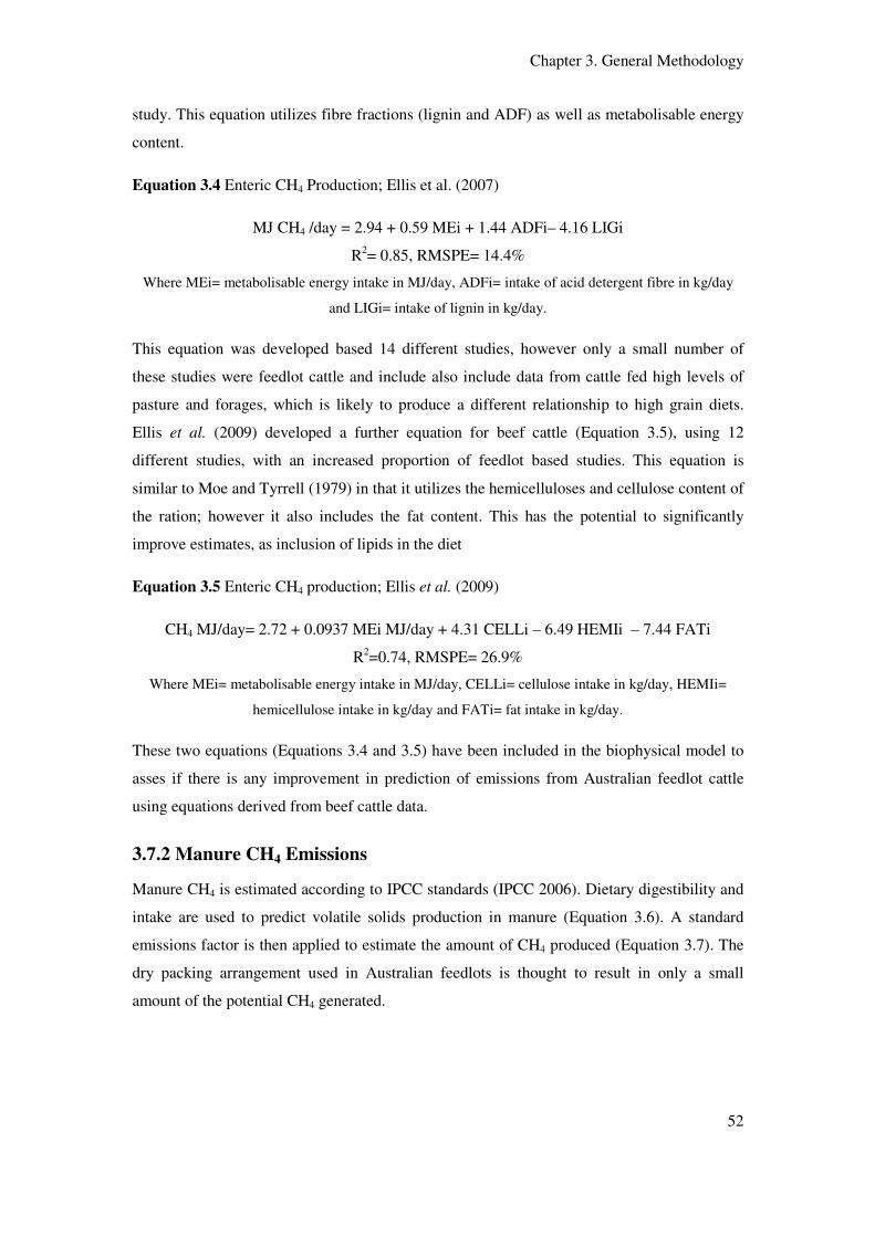
Chapter 3. General Methodology
52
study. This equation utilizes fibre fractions (lignin and ADF) as well as metabolisable energy
content.
Equation 3.4 Enteric CH4 Production; Ellis et al. (2007)
MJ CH4 /day = 2.94 + 0.59 MEi + 1.44 ADFi– 4.16 LIGi
R2= 0.85, RMSPE= 14.4%
Where MEi= metabolisable energy intake in MJ/day, ADFi= intake of acid detergent fibre in kg/day
and LIGi= intake of lignin in kg/day.
This equation was developed based 14 different studies, however only a small number of
these studies were feedlot cattle and include also include data from cattle fed high levels of
pasture and forages, which is likely to produce a different relationship to high grain diets.
Ellis et al. (2009) developed a further equation for beef cattle (Equation 3.5), using 12
different studies, with an increased proportion of feedlot based studies. This equation is
similar to Moe and Tyrrell (1979) in that it utilizes the hemicelluloses and cellulose content of
the ration; however it also includes the fat content. This has the potential to significantly
improve estimates, as inclusion of lipids in the diet
Equation 3.5 Enteric CH4 production; Ellis et al. (2009)
CH4 MJ/day= 2.72 + 0.0937 MEi MJ/day + 4.31 CELLi – 6.49 HEMIi – 7.44 FATi
R2=0.74, RMSPE= 26.9%
Where MEi= metabolisable energy intake in MJ/day, CELLi= cellulose intake in kg/day, HEMIi=
hemicellulose intake in kg/day and FATi= fat intake in kg/day.
These two equations (Equations 3.4 and 3.5) have been included in the biophysical model to
asses if there is any improvement in prediction of emissions from Australian feedlot cattle
using equations derived from beef cattle data.
3.7.2 Manure CH4 Emissions
Manure CH4 is estimated according to IPCC standards (IPCC 2006). Dietary digestibility and
intake are used to predict volatile solids production in manure (Equation 3.6). A standard
emissions factor is then applied to estimate the amount of CH4 produced (Equation 3.7). The
dry packing arrangement used in Australian feedlots is thought to result in only a small
amount of the potential CH4 generated.

Chapter 3. General Methodology
53
Equation 3.6 Volatile solids excretion
Volatile solids kg/day= i x (1- DMD) x (1- A)
Where i = intake, DMD= dry matter digestibility expressed as a fraction (assumed to be 0.8 for feedlot
diets) and A= ash content expressed as a fractions (assumed to be 0.08 for feedlot rations).
Equation 3.7 Methane production from manure
Manure CH4 kg/head/day= VS x B X MCF X ρ
Where VS= volatile solids (kg/day), B= the emissions potential of CH4 (-0.17m3 CH4/kg VS), MCF=
the CH4 conversion factor for the manure management system (for Northern Australia this value is 5%
and for Southern Australia this factor is 1.5%, based on climatic conditions). ρ = the density of CH
(0.662 kg/m3).
3.8 Nitrogen Model
There are two primary components to the N portion of the biophysical model. The equations
developed by the (SCA 1990 ) and Freer et al. (1997) as published in the National Inventory
Methodology (AGO 2006) are used to estimate N transactions within the animal; N retained
and excreted as urine and faecal N. The second component of the N model uses a set
emissions factor for the drylot management system to estimate the emission of N2O and
volatilisation of NH3.
The SCA (1990) methodology is used in the National Inventory Methodology (2006) as it was
developed in Australia and was therefore selected in preference to the IPCC standard (for N
excretion, which is based on NRC guidelines (NRC 1996). This method uses a mass balance
approach (N output= N input- N storage). This method for prediction N transactions was
selected for the model as it is the Australian standard for calculating nutrient requirements for
beef cattle, and as shown by its selection for the National Inventory Methodology (AGO
2006) over the IPCC standard values, is likely to form the basis of any methodology
estimating N transactions in cattle.
Nitrogen intake is calculated based on the crude protein concentration of the ration, with
crude protein considered a fixed 6.25 times N content. The N excreted in the faeces is
calculated (Equation 3.8) based on equations developed by the SCA (1990) and considered
the indigestible fraction of undegraded protein from feed, microbial protein and endogenous
faecal N.

Chapter 3. General Methodology
54
Equation 3.8 Faecal N Excretion
Faecal N g/head/day = (0.3(CPI x (1- ((DMD+ 10)/100)))+ 0.015 (ME x i x 0.008)+ (0.0152 x
i)/ 6.25
Where CPI= crude protein intake, DMD= dry matter digestibility, ME= metabolisable energy content
of the ration, i= intake and 6.25 represents a standard factor to convert crude protein to N.
Similarly, the amount of N retained in the body tissue is calculated (Equation 3.9) based on
growth rates and relative intake of the animal based on level of intake required for
maintenance and size of the animal relative to mature body size (based on a standard
reference weight, for feedlot cattle this is 660 kg, AGO 2006).
Equation 3.9 Nitrogen Retention
N retained g/head/day = ((0.212- 0.008 (Ri-1)- (0.140-0.008(L-2)/1+exp-6(z-0.04))) x (LWG x
0.92)) / 6.25
Where Ri= relative intake, determined by dividing feed intake by the intake required for maintenance,
Z= relative size and LWG= live weight gain.
Finally, urinary N excretion is calculated using a mass balance approach (Equation 3.10),
subtracting faecal N, retained N and dermal N loss from N intake.
Equation 3.10 Calculation of Urinary N excretion using a mass balance approach
Urinary N g/head/day= (CPi/ 6.25)- N Retained- Faecal N – ((1.1x 10⁻⁴x W0.75)/6.25)
Where CPi= crude protein intake, 6.25 represents a standard figure to convert nitrogen to crude protein
and W= live weight, with W0.75 = metabolic live weight
The second component of the N model uses standard emissions factors for drylot management
systems to convert the excreted N volatile NH3 and emitted N2O (Equations 3.11 and 3.12).
Equation 3.11 Estimated N2O Emissions from Faecal N
Faecal N2O g/head/day = Faecal N x MMS x EFmms x Cg
Equation 3.12 N2O Emitted from Urinary N

Chapter 3. General Methodology
55
Urine N2O g/head/day = Urinary N x MMS x EFmms x Cg
Where MMS indicates the fraction of manure managed under the manure management system (for
feedlot systems this is set at 1, with 100% of manure being managed under the dry lot management
system), EFmms = the N2O emission factor for the manure management system (for drylot manure
management systems the emission factor is 0.02. Cg is a factor used to convert the elemental mass of
N2O to molecular mass = 44/28.
Volatile NH3 is estimated in a similar way, with the fraction of NH3 volatilised under the
manure management system set as 0.03 for feedlot systems (Equations 3.13 and 3.14).
Equation 3.13 Loss of volatile NH3 from faecal N
Volatile Faecal N g/head/day= Faecal N x Fraction of N volatile
Equation 3.14 Loss of volatile NH3 from urinary N
Volatile Urinary N g/head/day= Urine N x fraction of N volatile
Where fraction of N volatile is set at 0.03 for feedlot systems
3.9 Assumptions
The assumptions primarily deal with the gross composition of the feed (digestibility, energy),
the conversion of energy to CH4 in the animal and manure and the emission of N2O and NH3.
The main assumptions used in the calculations are outlined in Table 3.3.
Emissions of nitrogenous gases and CH4 from manure are considered to be dependent on the
management of manure. For the purposes of the model all manure is assumed to be managed
under the dry lot management system. Emission factors for CH4 are taken from the Australian
Greenhouse Office (AGO 2006) (0.015 temperate, 0.05 warm) rather than the IPCC
guidelines (IPCC 2006). However emission factors for nitrogenous gases are taken from the
IPCC standard under the guidelines of the National Inventory Methodology (AGO 2006).
Detailed ration composition (cellulose, hemicelluloses and lignin) is not commonly reported,
or provided in ration information. Where these values were required for model calculations as
in Moe and Tyrrell (1979), Ellis et al. (2007) and Ellis et al. (2009), they were calculated
based on Givens and Moss (1990) and the Cornell net crude protein system (CNCPS; Sniffen
et al. 1992). This was required for all feed lignin and ADF values, as well as detailed
composition of some unusual feedstuffs (protein meals). The gross energy of individual feeds
is assumed to be 18.4, with a digestibility of 80% (AGO 2006).

Chapter 3. General Methodology
56
Some assumptions were required to be made about the production systems in order to classify
the output and provide information about basic management practices. There are assumed to
be three production categories short fed domestic (<100 days), short fed export (100-200
days) and long Fed Export (>200 days; AGO 2006, van Sliedregt et al. 2000). Cattle were
grouped into these classes based on data provided by the feedlot. This influences the standard
reference weight, and intakes which can be predicted using the class of cattle (as a
comparison to offered feed) based on van Sliedregt et al. (2000).
Table 3.3 Assumptions of the standard model
Parameter Set Value Source
Energy content of CH4 55.22 MJ/kg Brouwer (1965)
Density of CH4 0.662 kg/m3
Gross energy content of feed 18.4 MJ/kg DM SCA (1990 )
Dry Matter Digestibility 80 %
Ym (CH4 conversion factor) 3% IPCC (2006)
MCF (manure CH4) 0.015 temperate
0.05 warm AGO (2006)
EF N2O 0.02 kg N as N2O/ kg N IPCC (2006)
EF NH3 0.03 kg N as NH3/ kg N IPCC (2006)
3.10 Validation
The first stage of the modelling process was the validation (described in chapter 4) of the
various models using published data. Separate databases were developed for enteric CH4, N
transactions and N emissions.
3.10.1 Enteric CH4 Model
In order to evaluate the ability of the model to predict changes in emissions associated with
changes in parameters, published results were used to test the model. The basic model was
evaluated for its ability to reflect the physiological changes associated with changes in diet
and intake, primarily changes in digestibility and intake, and changes in the fermentation
products produced by different diet types (e.g. propionate dominant in a high grain diet vs.
acetate dominant in a high forage diet).
Full details of the studies selected for validation of the enteric CH4 emissions model can be
found in Chapter 4, Table 4.1. Briefly; studies in the database were published since 2000 and

Chapter 3. General Methodology
57
focused on manipulating dietary factors on CH4 emissions from feedlot cattle. The primary
factor under investigation was the energy density of the diet; high vs. low forage, with the
exception of Hegarty et al. (2007) which used the same ration at different intake levels.
Rations used in the CH4 validation (Table 4.2) studies ranged in forage proportion from 0.09
to 0.7. With ME values between 8.8 and 12.1 MJ/kg and CP from 120 to 150 g/kg. Animal
production data used in the validation of the enteric CH4 model is outlined in Table 4.3.
Animal live weights ranged between 360 and 640kg, with reported live weight grains of
between 0.6 and 1.8 kg/day. Corresponding intakes ranged between 5.34 and 14.13 kg
DM/day, with reported CH4 outputs of 62 to 192 g/head/day.
3.10.2 Nitrogen Model
As with the enteric CH4 model, a database of studies was created to validate the prediction
equations for nitrogenous gases under the Australian Inventory methodology (2006).
However, in contrast to the model for enteric CH4, the N model was validated in two stages;
primarily due to lack of data directly linking detailed animal and ration information to
measured emissions. Initially a database was created providing data about N transactions in
the animal and used to validate the equations predicting N intake, retention and excretion
(Table 4.4). A second database was created focussing on volatilisation of NH3 and emission
of N2O from feedlot manure (Table 4.7). Studies selected for the validation of the N excretion
model were published since 2000, and focused on changing the N concentration in the diet
and effects on N retention and excretion in feedlot cattle. Average live weight in these studies
ranged from 495 to 627 kg, with average growth rates between 0.92 and 1.76 kg/day. Intakes
ranged from 6.4 to 11.4 with corresponding N intakes of 94.3 to 240 g/day (Table 4.5).
Limited ration information was provided in these studies, with many reporting only CP and
ME content (Table 4.6). Where ration nutritive value was not provided it was calculated based
on Givens and Moss (1990). The database of studies examining the emissions of N2O and
volatilisation of NH3 contained data from six published studies (Table 4.7). All studies were
published since 2000, but varied in the emissions measurement method. The direct emission
of N2O from feedlot manure pad (compared with compost piles) has received limited
attention, therefore data available to validation this component of the model was limited to the
results of Boadi et al. (2004b). Further, many recent studies examining the volatilisation of
NH3 from feedlot systems have been conducted using atmospheric dispersion and
micrometeorological methods, therefore detailed information on the composition of the
manure pad, rations and animal performance was not consistently available. Full details of the
studies utilised in the validation of the N excretion and gas components of the model are
found in Chapter 4.

Chapter 3. General Methodology
58
3.11 Comparison with Australian Feedlot Measurements
Full details of the approach used to compare measured and modelled emissions from
Australian feedlots are outlined in Chapter 5. Briefly, campaigns information was collected
from the feedlot operators in the form of bunk sheets, lot sheets, rations and daily feed
amounts. This information was collected for a minimum of five days for each 14 day
measurement campaign. Information collected included number of head (cattle) in each pen,
animal sex, estimated weight on entry and at the report date, days on feed, cattle class, rations
and amounts of feed offered. The collected data was utilised as input for the model outlined in
the general methodology (Sections 3.6 to 3.10). Three of the described equations for
estimation of enteric CH4 (Ellis et al. 2007; Moe and Tyrrell 1979 and IPCC Tier II) were
utilised in the application of the model to this data, based on the results of Chapter 4. The
predicted emissions of CH4, NH3 and N2O were compared statistically to measured values.
3.12 Statistical Analysis
For both the validation and model application exercises, linear regression (Genstat v. 11 VSN
International) was used to examine relationships between measured and predicted emissions.
Lin’s concordance (Genstat v. 11 VSN International) was used to measure how well the
modelled data reproduces the original data set (Lin 1989; Lin 2000). Lin (1989) reports that
this approach can detect non-reproducability in cases where the Pearson’s correlation
coefficient or paired t-test may provide misleading results. The concordance coefficient is
calculated using a simple Pearson’s correlation coefficient (reported in text as the correlation
between the variables) and the slope and origin of the line, known as Cb. Full equations can be
found in Appendix 9.1.
The factor Cb indicates the how far the best-fit line deviates from the 45° line (indicator of
accuracy). The further Cb is from 1, the greater the deviation. The Person correlation
coefficient (p) measures how much each observatiobn deviates from the best-fit line. The
concordance correlation coefficient evaluates the degree to which pairs fall on the 45° line,
with measurements of accuracy (Cb) and precision (p). For a perfect 45° line Pc = 1,
In biological systems, a correlation of 0.6 can be considered acceptable, however in the
comparison between the models the relative values can be considered equally important.
3.12.1 Interpretation

Chapter 3. General Methodology
59
The results of a Lin’s concordance analysis can be interpreted utilising the values of
concordance and correlation. High correlation and concordance indicate high model accuracy,
with a strong relationship between measured and predicted values, and a slope close to the
line of unity. A high correlation coupled with a low concordance indicates that while there is
a strong relationship between measured and predicted values, there are likely to be systemic
bias or errors in the model. Low correlations and concordance indicate poor model
performance, but may be reflective of a small range of data.
3.13 Animal Behaviour
In order to examine the relationship between diurnal emission pattern and animal feeding
patterns observations of animal feeding behaviour were conducted in conjunction with the
final two measurement campaigns (winter 2007 and summer 2008) at each site. Emissions
were measured using the methods described in Sections 3.2, full details of the behavioural
observations can be found in Chapter 6.
3.13.1 Pen Selection
Pens of cattle were selected to be representative of the general feedlot population (based on
weight, days on feed and breed composition). Pens also needed to be located close to power
supply and in an area where the camera could be mounted to view the entire pen (Plate 3.3).
3.13.2 Observations
Video recording was used to make continuous observations of the pen from sunrise to sunset.
Due to the lack of lights observations were not possible during the night. Observations were
recorded at 10 minute intervals by stopping the video and counting the number of cattle at the
feed bunk, water trough (if visible), standing and lying. Walking and “other” behaviours were
determined by viewing 15 seconds either side of the 10 minute time point and counting the
number walking and undertaking activities classified as other (grooming, interacting with
another animal). Number ruminating was determined using the same interval, by randomly
selecting 20 animals and counting the number ruminating. The proportion determined using
this method was then multiplied to give total number ruminating.
Video recording was validated using manual observations during the winter measurement
periods by a single operator using a modified octave approach. The 12 hour period from
sunrise to sunset was divided into three hour blocks and manual observations undertaken by a
single operator for one of these three hour periods over four consecutive days. Observations
were made in the categories defined above.

Chapter 3. General Methodology
60
3.13.3 Animal Details
During the first (winter) measurement campaign at the Southern Site the pen contained 247
head of mostly B. Taurus steers, weight 434-442 kg, minimum 28 days on feed (DOF). The
ration fed contained 69.9% wheat, 12.5% silage, 3.5% grass hay, 5% liquid finisher, 8%
cottonseed and 1.1% veg oil. 75% DM, 14.42% CP, 13.15 MJ ME/kg DM. At the Northern
Site the pen contained 161 head of B. Indicus beef steers. Estimated weight of 477 kg,
approximately 30 DOF. The ration fed comprises 11.5% silage, 0.5% recycled oil, 1.5%
straw, 4.6% liquid supplement, 75.9% sorghum grain and 6% cottonseed. 69.15% DM,
13.50% CP, 12.76 MJ ME/kg DM.
During the second (summer) measurement campaign the Southern Site contained 223 head of
B. Taurus cattle, between 480 and 570kg and 60 to 75 days on feed. The ration fed contained
27% wheat, 14% silage, 1.5% grass hay, 4.8 % liquid finisher, 8% cotton seed, 1.1%
vegetable oil, 3.1% molasses and 40.5% barley. 73% DM, 13.5% CP, 12.8 MJ ME/ kg DM.
The Northern Site pen contained 196 head of B. Taurus steers, 642 kg, and 116 days on feed.
The ration fed contained 39% sorghum, 4.5 liquid supplement, 1% straw, 1% cotton hulls,
10% cotton seed, 5% silage, 39% barley and 0.5% recycled oil. 73% DM, 13.83% CP, 12.67
MJE ME/kg DM.
3.13.4 Statistical Analysis
Ten minute behavioural observations were averaged over 30 minute periods for comparison
with the emissions measurements (15 minute values averaged over 30 minute periods).
Simple correlation analysis was used to evaluate the relationship between emissions of CH4
and NH3, and animal feeding behaviour, as well as temperature (°C).

Chapter 3. General Methodology
61
A
B
Plate 3.3 Video camera mounted in the Northern (A) and Southern (B) feedlots

Chapter 4. Model Validation
62
Chapter 4. Evaluation of a Methodology for Estimation of
Greenhouse Gas Emissions from Feedlot Systems
4.1 Introduction
The Australian agricultural sector, like many other industries, faces considerable pressure to
reduce emissions of the greenhouse gases. However, in order to assess the usefulness of
mitigation options, current emissions need to be accurately measured and estimated.
Measurement of greenhouse gas emissions can be expensive and complicated (Ellis et al.
2007), however prediction equations can be used to estimate emissions. Empirical models
currently used in national inventories were developed in the 1960’s and 1970’s for
metabolism based predictions, and not for the greenhouse inventories. Therefore, the
predictions may not adequately reflect the Australian feedlot environment, particularly as
most are based on calorimetric measurements designed to measure the energy value of feeds
(Denmead et al. 2000) and not as a measurement of the contribution of these gases towards
global warming (Ellis et al. 2007). Additionally, empirical models often have variables which
are not commonly measured and many have been reported to be inaccurate for conditions
outside those (rations, animal characteristics etc) which were used in the development (Ellis et
al. 2007; Mills et al. 2003; Wilkerson et al. 1995).
The National Inventory Methodology (AGO 2006) for estimation of greenhouse sources and
sinks is used in Australia for carbon accounting under the Kyoto protocol, and would be the
likely basis for estimation under a future carbon constrained economy, such as the recently
proposed Carbon Farming Initiative (Austalian Government 2010a). However, the accuracy
of the Australian Inventory Methodology (AGO 2006) for feedlot systems has not been
evaluated under commercial Australian conditions. Furthermore reducing total N loss is
important for the sustainability of the feedlot industry (Erickson et al. 2000). However, as
with enteric CH4 emissions measurement nitrogenous gases in situ can be complicated and
expensive. Although emissions of NH3 do not currently have to be reported under the
UNFCCC guidelines, monitoring potential and actual NH3 emissions will become
increasingly important, particularly in terms of contribution to indirect N2O emissions.
4.1.1 Inventories and Emissions Reporting
According to international agreements under the United Nations Framework Convention on
Climate Change (UNFCCC), national inventories of greenhouse gas emissions are prepared
annually. These inventories are prepared according to published methodologies and allow
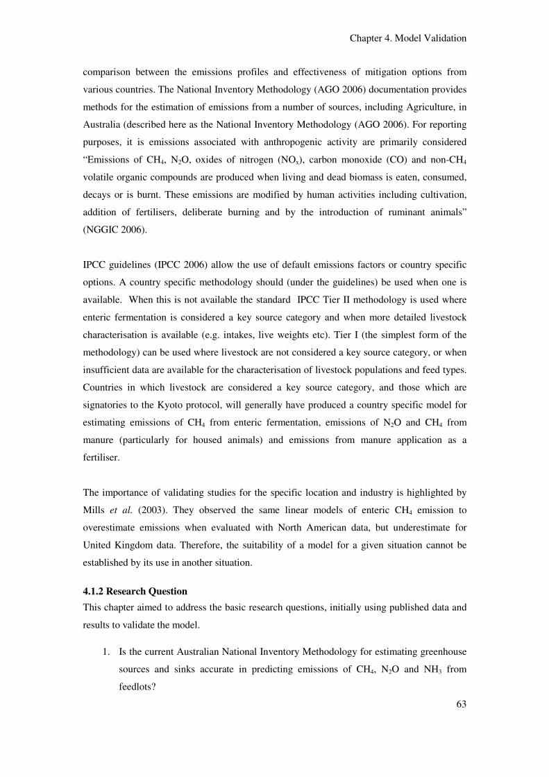
Chapter 4. Model Validation
63
comparison between the emissions profiles and effectiveness of mitigation options from
various countries. The National Inventory Methodology (AGO 2006) documentation provides
methods for the estimation of emissions from a number of sources, including Agriculture, in
Australia (described here as the National Inventory Methodology (AGO 2006). For reporting
purposes, it is emissions associated with anthropogenic activity are primarily considered
“Emissions of CH4, N2O, oxides of nitrogen (NOx), carbon monoxide (CO) and non-CH4
volatile organic compounds are produced when living and dead biomass is eaten, consumed,
decays or is burnt. These emissions are modified by human activities including cultivation,
addition of fertilisers, deliberate burning and by the introduction of ruminant animals”
(NGGIC 2006).
IPCC guidelines (IPCC 2006) allow the use of default emissions factors or country specific
options. A country specific methodology should (under the guidelines) be used when one is
available. When this is not available the standard IPCC Tier II methodology is used where
enteric fermentation is considered a key source category and when more detailed livestock
characterisation is available (e.g. intakes, live weights etc). Tier I (the simplest form of the
methodology) can be used where livestock are not considered a key source category, or when
insufficient data are available for the characterisation of livestock populations and feed types.
Countries in which livestock are considered a key source category, and those which are
signatories to the Kyoto protocol, will generally have produced a country specific model for
estimating emissions of CH4 from enteric fermentation, emissions of N2O and CH4 from
manure (particularly for housed animals) and emissions from manure application as a
fertiliser.
The importance of validating studies for the specific location and industry is highlighted by
Mills et al. (2003). They observed the same linear models of enteric CH4 emission to
overestimate emissions when evaluated with North American data, but underestimate for
United Kingdom data. Therefore, the suitability of a model for a given situation cannot be
established by its use in another situation.
4.1.2 Research Question
This chapter aimed to address the basic research questions, initially using published data and
results to validate the model.
1. Is the current Australian National Inventory Methodology for estimating greenhouse
sources and sinks accurate in predicting emissions of CH4, N2O and NH3 from
feedlots?

Chapter 4. Model Validation
64
2. Are equations based on energy or carbohydrate more accurate in estimating CH4
emissions?
3. What is the impact of using a single emissions factor in the model to predict NH3 and
N2O?
4. Does introducing equations developed based on beef cattle data improve accuracy of
estimates compared to measured values of CH4 emissions compared with the current
approaches?
5. How sensitive is the model to changes in parameters such as animal intake, and to
the gross energy and dietary digestibility of the ration?
4.2 Model Development/Structure
The full model is outlined in detail in the general methodology (Section 3.6 to 3.10). Breifly,
the concept of the model was to utilise the current National Inventory Methodology (AGO
2006 ) for estimating emissions (CH4, N2O and NH3) from feedlot cattle, with additional
equations for the prediction of enteric CH4 emissions (developed specifically for beef or
feedlot type cattle). This section will discuss the equations selected for the model, the
development of these original models, and the usefulness/ applicability of the parameters
which are used, in the context of a feedlot system.
An empirical modelling approach was used, as these types of models will allow data which is
collected in a commercial environment (or for which reasonably reliable tabulated data exist)
to be utilised as inputs. The alternative approach is a dynamic mechanistic model- which
attempts to represent rumen fermentation biochemistry and processes (Mills et al. 2003).
Although this type of model can provide much more accurate estimates, they require more
complex information and do not enable estimates based on limited dietary information (Mills
et al. 2003). The complexity of these models makes them unsuitable for application in a
commercial environment or for use in updating National Inventory guidelines, where an
empirical model is a more practical approach.
4.2.1 IPCC Tier I and Tier II Equations
The IPCC recommend the use of a Tier II country specific model for ‘other’ (non dairy)
cattle, including feedlot cattle (IPCC 2006). However, it is valid to compare emissions
calculated using the standard Tier II methodology and the single estimate used in Tier I with
values measured for feedlot cattle for two reasons. Firstly, the Tier II approach is utilised in
countries where agriculture is not considred a key source category, many of which have large

Chapter 4. Model Validation
65
feedlot industries Secondly, feedlot production is increasing in developing countries, where
there is likely to be insufficient information (animal population, production system
characteristics and feed base details) to utilise a Tier II approach or more detailed country
specific approach. Increasing understanding of the accuracy of these models for feedlot
production will be beneficial in the ability to compare industries.
The Tier I methodology is based on cattle type and geographical region. Oceania is
characterised as having “Commercialised dairy sector based on grazing. Separate beef cow
herd, primarily grazing rangelands of widely varying quality with growing amount of feedlot
feeding with grains”(IPCC 1996). Under the IPCC Tier I methodology beef cattle are
estimated at producing 60 kg CH4/head/year, equating to 164 g CH4/head/day, assuming a
calendar year.
Tier II is the simplest step of the methodology which allows differences in animal production
systems to be accounted for. The IPCC standard Tier II methodology estimates gross energy
intake based on dry matter intake and a standard value for the gross energy content of feeds.
Gross energy intake is multiplied by a set factor for CH4 as a percentage of GEi, with
different factors for different production systems. For a feedlot system, 3 ±1 % of GEi is
assumed to be emitted as CH4, compared with 6.5 ±1 % for dairy and grazing beef systems. A
criticism of this method is that a single factor is not representative of the proportion of gross
energy converted to CH4 for all feed types and production systems. Measurements from
feedlot systems and from beef cattle fed feedlot type rations suggest emissions ranging from
62 g/head/day to190 g/head/day, or between 0.7 and 7.3 % GEi (Beauchemin and McGinn
2005; Boadi et al. 2004b). Even with a single diet type considerable variability has been
observed; Boadi et al. (2004b) measured CH4 production, as a percentage of GE, as between
0.9 and 6.9% for a high forage feedlot diet, and from 0.7 to 4.9% for a high grain diet. In this
evaluation a figure of 3% of gross energy intake, and 18.4 MJ/ kgDM of gross energy are
used, in accordance with the IPCC standard for feedlot cattle.
4.2.2 Moe and Tyrell (1979) Equation
This equation (Equation 3.2) is used as the Australian country specific model for beef feedlot
cattle (Tier II, country specific), as it is considered to better represent the type of diets fed to
feedlot cattle (higher grain/ concentrate) compared with a methodology based on energy and
intake. Moe and Tyrell (1979) developed this equation based on studies with dairy cows,
with the original experiments designed to examine the effects of dietary components (protein,
concentrate proportion, different grain types, and form of grain) on energy utilisation in dairy

Chapter 4. Model Validation
66
cattle diets. In the studies utilised in the development of the Moe and Tyrrell (1979) model all
animals were Holstein dairy cows, with live weight ranging from 369 to 893 kg (average 617
kg), and corresponding intakes 2.7 to 22.9 kg DM/day (average 12.1 kg DM/day). The range
of diets included corn and barley grain, oats, beet pulp, dried brewers grains and dried
distillers grains.
Moe and Tyrrell (1979) report that the soluble residue (calculated as neutral detergent soluble
minus crude protein and ether extract) utilised in the equation should represent most soluble
and readily fermentable carbohydrates, consisting primarily of starch for the mixed rations
evaluated. The other parameters of interest are cellulose (ADF- lignin and silica) and
hemicellulose (NDF-ADF). Which were determined to have the most significant relationships
with CH4 production (other dietary parameters (crude protein, ether extract and lignin were
determined to be non significant). Intake of soluble residue ranged from 0.95 to 9.66 kg/day
(average 5.06 kg/day), cellulose from 0.41 to 3.90 kg/day and hemicellulose from 0.47 to 4.41
kg/day. CH4 production as a percentage of GEi averaged 6.3% (1.6 to 9.9%).
The equation of Moe and Tyrrell (1979) is reported to have the advantage of utilising a wider
range of rations than many other studies (e.g. Blaxter and Clapperton 1965). The basis of the
equation on carbohydrate fractions additionally means that it is able to distinguish differences
in emissions associated with changes in diet type. Variation in emissions from diets with
different digestibility, diets increasing in grain content, and from different basal grains are
commonly reported (Beauchemin and McGinn 2005; Boadi et al. 2004b); using an equation
with a set value for GE or digestibility does not allow these differences to be distinguished.
A detailed review of a number of statistical models by Wilkerson et al. (1995) suggested that
Moe and Tyrrell (1979) should be used for dairy cattle, however, as noted by Mills et al.
(2003) this was developed based on North American data and therefore may not represent
other feed types or animal genetics. Mills et al. (2003) observed this model to be the best
estimate for both North American and United Kingdom data, and suggests its use for dairy
cattle, making no recommendation for beef cattle. A disadvantage of more specific dietary
approaches; is that parameters (such a cellulose, hemicellulose) are not commonly measured,
in both commercial feed tests and for research purposes (Mills et al. 2003). Additionally,
values for these feeds may vary considerably both between and within feed types and with
measurement methods, which may increase the error associated with using a set value for
emissions.

Chapter 4. Model Validation
67
4.2.3 Blaxter and Clapperton (1965) Equation
This equation (Equation 3.3) uses intake of dry matter digestibility and relative intake to
estimate Ym (a CH4 conversion factor). This is then multiplied by the intake of gross energy to
determine daily CH4 emissions (g/head/day). This equation was developed primarily based on
sheep (16 sources, cattle contributing only five sources) which are likely to vary significantly
from cattle, particularly those with high growth rates, (or high milk production) in terms of
CH4 emissions. The data set included 55 diets. CH4 production as a percentage of dietary
energy ranged from 6.2 to 10.8%. Primarily the diets were roughage based (29 diets), while
the mixed diets (11 diets) also contained some hay.
A downfall of this equation as used in the current National Inventory Methodology (AGO
2006) (Tier II) country specific model for dairy and grazing beef cattle) is that a set value is
given for both digestibility (80%) and feed gross energy content (18.4 MJ/kg DM).
Digestibility and energy content varies not only between feeds (e.g. forages lower in both
digestibility and energy than grains) but within single feeds. This limits the ability of this
methodology to distinguish between differing diet composition.
4.2.4 Ellis et al. (2007) Equation
Ellis et al. (2007) developed a range of equations for beef and dairy cattle, using dietary
variables. The source data utilised for this equation included both beef and dairy cattle,
entirely of Canadian and North American origin, DMI ranged from 3.8 to 18.4 kg DM/day,
live weights between 268 and 707 kg. Mean forage percentage in the beef rations was 79% (9
to 100%) and in the dairy rations 69% (28 to 100%). At the lower end this is similar to feedlot
type diets, however the number of high grain diets evaluated was not reported. The best
performing equation for beef cattle (Equation 3.4) uses dietary NDF, lignin and metabolisable
energy intake (MEi), similar in principal to Moe and Tyrell (1979). The primary advantage of
this equation is that a database focussed specifically on beef cattle was used in the
development, which can be assumed to increase accuracy.
However Yan et al. (2009) determined high predictive error when validating a range of
prediction equations developed by Ellis et al. (2007), with the lowest R2 values (in their
study) recorded for these set of equations. They attributed this to the use of both calorimetric
(20 sources), SF6 (8 sources) and mass balance (one source) methods in the measurements
used for the producing the equations. This will be discussed in more detail in the general
discussion, however observations (Boadi et al. 2004b; Grainger et al. 2007) suggest that there
are significant differences in CH4 emissions measured using chambers and SF6 techniques,
even when feed type and intake is constant.
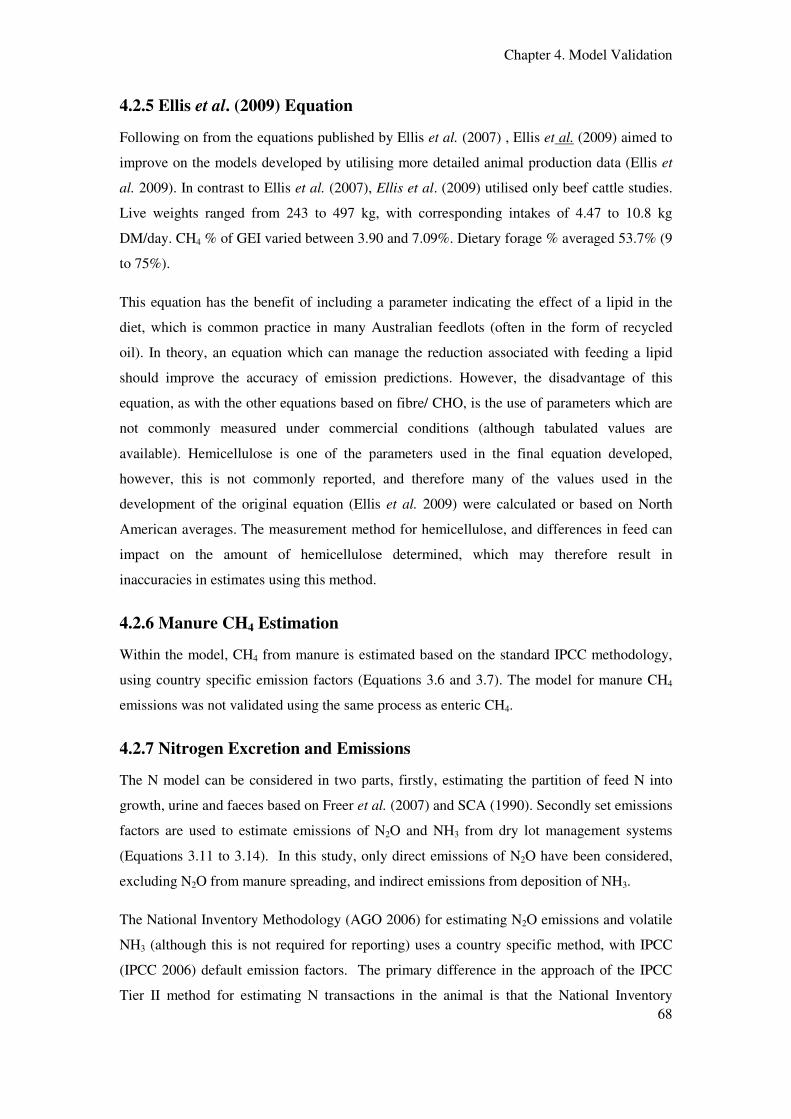
Chapter 4. Model Validation
68
4.2.5 Ellis et al. (2009) Equation
Following on from the equations published by Ellis et al. (2007) , Ellis et al. (2009) aimed to
improve on the models developed by utilising more detailed animal production data (Ellis et
al. 2009). In contrast to Ellis et al. (2007), Ellis et al. (2009) utilised only beef cattle studies.
Live weights ranged from 243 to 497 kg, with corresponding intakes of 4.47 to 10.8 kg
DM/day. CH4 % of GEI varied between 3.90 and 7.09%. Dietary forage % averaged 53.7% (9
to 75%).
This equation has the benefit of including a parameter indicating the effect of a lipid in the
diet, which is common practice in many Australian feedlots (often in the form of recycled
oil). In theory, an equation which can manage the reduction associated with feeding a lipid
should improve the accuracy of emission predictions. However, the disadvantage of this
equation, as with the other equations based on fibre/ CHO, is the use of parameters which are
not commonly measured under commercial conditions (although tabulated values are
available). Hemicellulose is one of the parameters used in the final equation developed,
however, this is not commonly reported, and therefore many of the values used in the
development of the original equation (Ellis et al. 2009) were calculated or based on North
American averages. The measurement method for hemicellulose, and differences in feed can
impact on the amount of hemicellulose determined, which may therefore result in
inaccuracies in estimates using this method.
4.2.6 Manure CH4 Estimation
Within the model, CH4 from manure is estimated based on the standard IPCC methodology,
using country specific emission factors (Equations 3.6 and 3.7). The model for manure CH4
emissions was not validated using the same process as enteric CH4.
4.2.7 Nitrogen Excretion and Emissions
The N model can be considered in two parts, firstly, estimating the partition of feed N into
growth, urine and faeces based on Freer et al. (2007) and SCA (1990). Secondly set emissions
factors are used to estimate emissions of N2O and NH3 from dry lot management systems
(Equations 3.11 to 3.14). In this study, only direct emissions of N2O have been considered,
excluding N2O from manure spreading, and indirect emissions from deposition of NH3.
The National Inventory Methodology (AGO 2006) for estimating N2O emissions and volatile
NH3 (although this is not required for reporting) uses a country specific method, with IPCC
(IPCC 2006) default emission factors. The primary difference in the approach of the IPCC
Tier II method for estimating N transactions in the animal is that the National Inventory

Chapter 4. Model Validation
69
Methodology (AGO 2006) is based on the equations developed by SCA (1990), while the
IPCC model is based on the NRC (1996). However, the underlying approach of both
methodologies is similar, with a mass balance approach of N intake- N Retention= N
excretion utilised. The SCA models partition N excretion into faecal and urinary N, while the
IPCC methodology uses a single figure for N excretion.
4.3 Methods
The enteric CH4 component of the model was evaluated using the results of published studies.
The procedure followed will be discussed in more detail in the following sections, however
briefly, a database was developed comprising studies which focussed specifically on enteric
CH4 emissions from beef feedlot cattle. Where data were not available specifically for beef
feedlot cattle, the database was extended to include beef cattle with similar characteristics to
feedlot cattle (weight, age, ration types, intakes).
The N model was validated in two stages. Initially a database was created providing data
about N transactions in the animal and used to validate the equations predicting N intake,
retention and excretion (in manure and faeces). A second database was created focussing on
volatilisation of NH3 and emission of N2O from feedlot manure.
4.3.1 Enteric CH4 Validation
Five published studies were selected for the validation of the enteric CH4 model (Table 4.1).
These studies all investigated the effect of changing dietary parameters (chemical
composition, intake) on enteric CH4 emissions. One study Boadi et al. (2004b) included data
on emissions of CH4 and N2O from manure. Studies in the database were published since
2000 and focused on manipulating dietary factors on CH4 emissions from feedlot cattle. The
primary factor under investigation was the energy density of the diet, utilizing high and low
forage proportion, with the exception of Hegarty et al. (2007) who utilized the same ration at
different intake levels.
Table 4.1 Studies selected for evaluation of the standard model, comparisons of the model
and physiological response tested in the model
Study Primary Comparison
Beauchemin and McGinn (2005) Backgrounding v. Finishing
Boadi et al. (2004b) High Forage vs. Low Forage
Beauchemin and McGinn (2006) Level of Grain
Hegarty et al. (2007) Intake

Chapter 4. Model Validation
70
Lovett et al. (2003) Forage: concentrate ratio
The studies (Table 4.1) were primarily conducted in the Northern hemisphere, with the
exception of Hegarty et al. (2007). There are limited studies investigating changes in dietary
parameters on CH4 emissions of feedlot cattle under Australian conditions, therefore Northern
hemisphere based studies were also included. Rations used in the CH4 validation studies
ranged in forage proportion from 0.09 to 0.7. ME values ranged between 8.9 and 12.1 MJ/kg
DM and CP from 120 to 150 g/kg DM. Forage proportion ranged between 9 and 70% of the
rations. Animal live weights ranged between 360 and 640kg, with reported live weight grains
of between 0.6 and 1.8 kg/day. Corresponding intakes ranged between 5.3 and 14.1 kg
DM/day, with reported CH4 outputs of 62 to 192 g/head/day (Table 4.3).

Chapter 4. Model Validation
71
Table 4.2 Ration characteristics of the studies utilised for validation of the enteric CH4 model
^ study included an investigation of the effects of inclusion of coconut oil into the above rations, however for simplicity only the results of alteration to the forage
concentration of the diet were utilized. * offered forage proportion, #reported as GE kcal/kg DM ME calculated using digestibility of GE and a factor of 4.184 to
convert kcal to MJ, ˜ reported as GE KJ/g ME calculated.
Study Ration DM
%
GE
MJ/kg
ME
MJ/ kg
CP
g/kg DM
NDF
g/kg DM
ADF
g/kg DM
Forage
Proportion*
Corn Backgrounding 50.8 18.3 8.9# 146 350 150 0.70
Barley Backgrounding 42.2 18.6 9.4# 137 363 163 0.70
Corn Finishing 78.2 18.2 10.9# 134 127 35 0.09
Beauchemin and McGinn (2004)
Barley Finishing 78.2 18.1 10.6# 151 204 60 0.09
Low F:G 73.9 17.8 11.5˜ 132 196 102 0.11 Boadi et al. (2004b)
High F:G 55.6 18.8 10.6˜ 120 291 185 0.41
Low Grain 50.9 18.7 9.6# 168 348 218 0.70 Beauchemin and McGinn (2006)
High Grain 66.8 18.7 10.8# 160 203 116 0.30
Hegarty et al. (2007) 88.7 17.8 12.1 159 178 79 0.10
1 (65:35 F:C) 45.8 19.5 11.0˜ 158 473 272 0.60
2 (40:60) 60.2 18.8 10.5˜ 157 371 197 0.38
Lovett et al. (2003)^
3 (10:90) 77.9 17.9 10.˜ 155 244 104 0.12

Chapter 4. Model Validation
72
Table 4.3 Published animal production data and measured enteric CH4 emissions used in validation of the model (mean and standard deviation)
Study Ration/ Parameter Enteric CH4
g/head/day
Initial
Weight
Kg
Final
Weight
kg
ADG’
kg/day
Intake
kgDM/day
Days
on
Feed
FCE#
kg/ kgDMI
Corn Backgrounding 170 ± 22.3 330 ± 19.8 380 ± 25.5 1.2 ± 0.3 6.9 ± 1.60 42 0.17
Barley Backgrounding 130 ± 22.3 325 ± 19.8 364 ± 25.5 0.9 ± 0.3 5.3 ± 1.60 42 0.17
Corn Finishing 62 ± 22.3 426 ± 19.8 452 ± 25.5 0.8 ± 0.3 6.8 ± 1.60 32 0.11
Beauchemin and McGinn (2005)
Barley Finishing 80 ± 22.3 412 ± 19.8 442 ± 25.5 0.9 ± 0.3 6.2 ± 1.60 32 0.15
Low F:G 126± 47.0^ 300 ± 32.0 569 ± 37.0 1.8 ± 0.2 11.7 ± 3.00 150 0.15 Boadi et al. (2004b)
High F:G 90.± 47.0^ 302 ± 32.0 548 ± 37.0 1.5 ± 0.2 10.0 ± 3.00 164 0.15
Low Grain 132 ± 39.6 328 ± 28.0 430 ± 29.0 1.7* 6.2 ± 1.20 60 0.27 Beauchemin and McGinn (2006)
High Grain 151 ± 39.6 328 ± 28.0 430 ± 29.0 1.7* 7.5 ± 1.20 60 0.22
Ad Lib 169 ± 39.6 328 ± 28.0 430 ± 29.0 1.7* 8.3 ± 1.20 60 0.20
Restricted 114 ± 39.6 328 ± 28.0 430 ± 29.0 1.7* 5.4 ± 1.20 60 0.32
Low Intake 142± 52.2 541 ± 44.4 642 ± 52.1 1.1 ± 0.3 8.4 ± 2.60 15 0.13 Hegarty et al. (2007)
High Intake 190 ± 52.2 541 ± 44.4 642 ± 52.1 1.2 ± 0.3 14.1 ± 2.60 15 0.08
1 (65:35 F:C) 148 ± 120.0^ 463 ± 12.0 512 ± 30.0 0.6 ± 0.6 6.9 ± 2.04 77 0.09
2 (40:60) 193 ± 120.0^ 462 ± 12.0 525 ± 30.0 0.8 ± 0.6 8.4 ± 2.04 77 0.09
Lovett et al. (2003)
3 (10:90) 122 ± 120.0^ 462 ± 12.0 543 ± 30.0 1.1 ± 0.6 8.2 ± 2.04 77 0.13
*ADG (average daily gain) and days on feed not reported 60 days assumed based on class of cattle, ADG calculated based on weight gain and days on
feed, ^reported in L/head/day, #feed conversion efficiency calculated as kg of gain/ kg feed intake, ‘average daily gain

Chapter 4. Model Validation
73
4.3.2 Nitrogen Transactions
Studies selected for the validation of the N transaction model (Table 4.4) were published
since 2000, and focussed on changing the N concentration in the diet and effects on N
retention and excretion in feedlot cattle. Average live weight (Table 4.5) in these studies
ranged from 495 to 627 kg, with average growth rates between 0.9 and 1.8 kg/day. Intakes
ranged from 6.4 to 11.4 kg DM with corresponding N intakes of 94 to 240 g/day. Limited
ration information (Table 4.6) was provided in these studies, with many reporting only CP
and ME content. Where ration nutritive value was not provided it was calculated based on
ration composition and tabulated values (Givens and Moss 1990).
Table 4.4 Studies selected for validation of the model for nitrogen transactions in the animal
and primary parameter investigated
Source Primary Comparison
Cole et al. 2003 Crude Protein concentration
Adams et al. 2004 Digestibility of protein
Cole et al. 2006 Crude protein concentration
Archibeque et al. 2007 Crude protein concentration
Vasconcelos et al. 2009 Crude protein and urea level
The database of studies examining the emissions of N2O and volatilisation of NH3 contained
data from six published studies (Table 4.7). All studies were published since 2000, but varied
in the emissions measurement method. The direct emission of N2O from feedlot manure pad
(compared with compost piles) has received limited attention, therefore data available to
validation this component of the model was limited to the results of Boadi et al. (2004b).
Further, many recent studies examining the volatilisation of NH3 from feedlot systems have
been conducted using atmospheric dispersion and micrometeorological methods, therefore
detailed information on the composition of the manure pad, rations and animal performance
was not consistently available. For these studies, an estimate of N intake based on the data
provided in the publication was used in the model to predict NH3 volatilisation (Table 4.8).

Chapter 4. Model Validation
74
Table 4.5 Animal production data used in the validation of the model for nitrogen transactions (mean and standard deviation)
Study Trt. Initial
Weight
kg
Final
Weight
kg
ADG
kg/day
Days on
Feed
N
Intake
g/day
N
Retained
g/day
Faecal
N
g/day
Urine
N
g/day
Cole et al. (2003)^ 12% CP 404 ± 23.4 495# 1.6 ± 0.36 56 198 ± 29.1 22 ±7.38 29 ± 11.6 147 ± 25.9
14% CP 404 ± 23.4 517# 2.0 ± 0.36 56 240 ± 29.1 27 ±7.38 31 ± 11.6 182 ± 25.9
T1. Con 324 ± 9.8 613 ± 78.4 1.6 ± 0.39 180 211 ± 5.9 26 ± 0.98 91 ± 15.7*
T1. Bran 325 ± 9.8 591 ± 78.4 1.5 ± 0.39 180 221 ± 5.9 24 ± 0.98 93 ± 15.7*
T2. Con 376 ± 9.8 574 ± 39.2 1.5 ± 0.29 132 236 ± 9.8 27 ± 1.37 79 ± 12.7*
T2. Bran 376 ± 9.8 569 ± 39.2 1.5 ± 0.29 132 239 ± 9.8 27 ± 1.37 91 ± 12.7*
T3. Con 335 ± 9.8 627 ± 22.5 1.8 ± 0.10 166 291 ± 3.9 36 ± 0.59 98 ± 7.8*
Adams et al.
(2004)^
T3. Bran 337 ± 9.8 616 ± 22.5 1.7 ± 0.10 166 222 ± 3.9 34 ± 0.59 138 ± 7.8*
Cole et al. (2006)^ 11.5% CP 315 ± 12.3 561 ± 9.4 1.4 ± 0.03 180 135 ± 8.0 23 ± 1.16 41 ± 8.4 71 ± 8.1
13% CP 315 ± 12.3 570 ± 9.4 1.5 ± 0.03 180 167 ± 8.0 23 ± 1.16 58 ± 8.4 86 ± 8.1
Low 305 ± 57.6 507 ± 127.2 1.0 ± 0.84 184 94 ± 51.6 35 ± 48 37 ± 18 24 ± 37.2
Medium 307 ± 57.6 590 ± 127.2 1.5 ± 0.84 184 131 ± 51.6 50 ± 48 43 ± 18 39 ± 37.2
Archibeque et al. (2007)^
High 304 ± 57.6 588 ± 127.2 1.5 ± 0.84 184 143 ± 51.6 40 ± 48 43 ± 18 60 ± 37.2
T1. 11.5 315 ± 16.6 507 ± 67.5 1.24‘ 154 112 ± 16.6 39± 6.8 35 ± 31.4 38 ± 79.2
T1. 13 315 ± 16.6 507 ± 67.5 1.24’ 154 131 ± 16.6 37± 6.8 38 ± 31.4 55 ± 79.2
T1. 14.5 315 ± 16.6 507 ± 67.5 1.24’ 154 142 ± 16.6 42± 6.8 40 ± 31.4 60 ± 79.2
T2. 11.5 353 ± 43.6 499 ± 67.5 0.92’ 159 112 ± 16.6 39± 6.8 35 ± 31.4 38 ± 79.2
T2. 13 353 ± 43.6 499 ± 67.5 0.92’ 159 131 ± 16.6 37± 6.8 39 ± 31.4 55 ± 79.2
Vasconcelos
et al. (2009)^
T2. 14.5 353 ± 43.6 499 ± 67.5 0.92’ 159 142 ± 16.6 42± 6.8 40 ± 31.4 60 ± 79.2
* total manure N, ^ SEM reported S.D shown are calculated values, #calculated from daily gain and days on feed; blank areas represent data which was not reported
and could not be calculated based on published values, ‘ ADG (average daily gain) not reported, calculated from total gain and days on feed

Chapter 4. Model Validation
75
Table 4.6 Ration details of the studies used in the validation of the model for nitrogen
transactions
Study Treatment ME
MJ/kg DM
CP
g/kg DM
Cole et al. (2003) 12% CP 12.9 121
14% CP 12.8 141
Adams et al. (2004) T1. Control 12.0 129
T1. Bran 11.0 131
T2. Control 12.2 138
T2. Bran 10.9 138
T3. Control 12.0 127
T3. Bran 11.1 128
Cole et al. (2006) 11.5% CP 11.9 111
13% CP 11.7 131
Low 12.9 91 Archibeque et al. (2007))
Medium 12.9 117
High 12.9 139
Vasconcelos et al. (2009) T1. 11.5 11.8 104
T1. 13 11.9 104
T1. 14.5 11.6 115
T2. 11.5 11.7 115
T2. 13 11.5 128
T2. 14.5 11.6 128
The studies used in the validation of the N emissions component of the model utilised both
chamber (in vitro) and micrometeorological methods (Table 4.7). For the chamber studies N
intake ranged from 94 to 150 g/day with between 673 and 1277 g of N applied to the
chamber. For the micrometeorological studies N intake ranged from 160-205 g/head/day.

Chapter 4. Model Validation
76
Table 4.7 Studies selected for the validation of the model for nitrogen gas, major gas
measured and measurement approach
Source Gas Measured Measurement Method
Boadi et al. (2004b) N2O Chambers
Cole et al. (2005) NH3 Chambers
McGinn et al. (2007) NH3 Open-path Laser
Todd et al. (2008) NH3 Acid Washing Samplers
Van Haarlem et al. (2008) NH3 Open-path Laser

Chapter 4. Model Validation
77
Table 4.8 Treatments, N intakes and excretion and measured N emissions (N2O and NH3) used in the validation of the N gas model
Treatment N Intake
g/head/day
N Added
to Chamber
g
Faecal
N Added
g
Urine
N Added
g
NH3- Loss
g/head/day
N2O- Loss
g/head/day
Boadi et al. (2004b) Low forage: grain 98.1 0.16
High forage:
Grain 76.2 0.15
Cole et al. (2005) 11.5% CP 129.2 840 382 459 17.55
13% CP 143.3 1155 434 721 35.09
14.5% CP 150.4 1113 466 647 29.41
McGinn et al. (2007) Whole Feedlot 164 140
Todd et al. (2008) Summer 2002 162 117
Winter 2003 169 51
Summer 2003 186 130
Winter 2004 201 84
Summer 2004 205 131
Spring 2005 193 118
Van Haarlem et al (2009) Whole feedlot 318
blank areas represent data which was not reported and could not be calculated based on published values, ^ SEM. reported, SD calculated
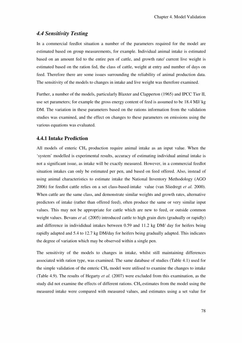
Chapter 4. Model Validation
78
4.4 Sensitivity Testing
In a commercial feedlot situation a number of the parameters required for the model are
estimated based on group measurements, for example. Individual animal intake is estimated
based on an amount fed to the entire pen of cattle, and growth rate/ current live weight is
estimated based on the ration fed, the class of cattle, weight at entry and number of days on
feed. Therefore there are some issues surrounding the reliability of animal production data.
The sensitivity of the models to changes in intake and live weight was therefore examined.
Further, a number of the models, particularly Blaxter and Clapperton (1965) and IPCC Tier II,
use set parameters; for example the gross energy content of feed is assumed to be 18.4 MJ/ kg
DM. The variation in these parameters based on the rations information from the validation
studies was examined, and the effect on changes to these parameters on emissions using the
various equations was evaluated.
4.4.1 Intake Prediction
All models of enteric CH4 production require animal intake as an input value. When the
‘system’ modelled is experimental results, accuracy of estimating individual animal intake is
not a significant issue, as intake will be exactly measured. However, in a commercial feedlot
situation intakes can only be estimated per pen, and based on feed offered. Also, instead of
using animal characteristics to estimate intake the National Inventory Methodology (AGO
2006) for feedlot cattle relies on a set class-based-intake value (van Sliedregt et al. 2000).
When cattle are the same class, and demonstrate similar weights and growth rates, alternative
predictors of intake (rather than offered feed), often produce the same or very similar input
values. This may not be appropriate for cattle which are new to feed, or outside common
weight values. Bevans et al. (2005) introduced cattle to high grain diets (gradually or rapidly)
and difference in individidual intakes between 0.59 and 11.2 kg DM/ day for heifers being
rapidly adapted and 5.4 to 12.7 kg DM/day for heifers being gradually adapted. This indicates
the degree of variation which may be observed within a single pen.
The sensitivity of the models to changes in intake, whilst still maintaining differences
associated with ration type, was examined. The same database of studies (Table 4.1) used for
the simple validation of the enteric CH4 model were utilised to examine the changes to intake
(Table 4.9). The results of Hegarty et al. (2007) were excluded from this examination, as the
study did not examine the effects of different rations. CH4 estimates from the model using the
measured intake were compared with measured values, and estimates using a set value for

Chapter 4. Model Validation
79
cattle class, intake as a % of live weight and intake calculated using an equation developed to
predict forage intake from size and growth of beef cattle (Minson and McDonald 1987).
4.4.2 Gross Energy Estimation
The common value assigned for the gross energy content of feeds is 18.4 MJ/ kg DM.
However, feeds commonly used in the feedlot range in GE content from 14.7 MJ/kg DM
(grass silage) to 39.3 MJ/ kg DM (oils; Givens and Moss 1990). Weighted average GE
concentrations were calculated using the data reported by Givens and Moss (1990) for the
rations in the validation studies. Measured and weighted average gross energy contents were
then used as inputs to the modelled equations, to examine the impact of the altered GE on
predicted CH4 emission. As discussed previously, there are two predominant kinds of
equations used in the modelling process, the energy based models (Blaxter and Clapperton
1965 and IPCC Tier II) and carbohydrate based models (Moe and Tyrrell 1979; Ellis et al.
2007 and Ellis et al. 2009). The carbohydrate based equations do not incorporate an estimate
of gross energy therefore the effect of changes to gross energy content was only examined on
the equations which utilise GE as a specific input parameter

Chapter 4. Model Validation
80
Table 4.9 Variation in predicted intake for a number of studies based on a set class based value, the equation of Minson and McDonald (1987), and a value
derived from percentage live weight.
Intake inputs
kgDM/head/day
Study Ration As Fed Method. Minson % LWT
Corn Backgrounding 6.9 9.8 8.5 9.1
Barley Backgrounding 5.3 9.8 7.8 8.7
Corn Finishing 6.8 9.8 8.8 10.8 Beauchemin and McGinn (2005)
Barley Finishing 6.7 9.8 8.9 10.6
Boadi et al. (2004b) Low F:C* 11.7 9.8 12.2 13.7
High F:C* 10.0 9.8 13.2 13.2
Low Grain 6.2 9.8 10.2 10.3 Beauchemin and McGinn (2006)
High Grain 7.5 9.8 10.2 10.3
Lovett et al. (2003) 1 (65:35 F:C*) 6.9 11.7 9.35 11.4
2 (40:60 F:C*) 8.4 11.7 9.38 11.4
3 (10:90 F:C*) 8.2 11.7 9.38 11.4
*F: C = forage to concentrate ratio

Chapter 4. Model Validation
81
4.5 Results
4.5.1 Enteric CH4
A significant (P<0.05) linear relationship was determined only for prediction based on Moe
and Tyrrell (1979) (Table 4.10). This is consistent with visual observations (Figure 4.1 and
4.2) indicating Moe and Tyrrell (1979) appears to have the best fit.. Based on concordance
(Table 4.11), the best estimates of CH4 emission are those based on the CHO based equations
of Moe and Tyrrell (1979) (0.26) and Ellis et al. (2007) (0.29), although concordance values
are low. The highest correlation was observed for Moe and Tyrell (1979) (0.63). This
suggests that for feedlot cattle, an equation which is able to represent the feed characteristics
will provide the most accurate estimate and allow the reduction in emissions associated with a
high grain diet to be fully represented.
Table 4.10 Fitted Linear relationships between measured and predicted CH4 emissions based
on five equations utilising the results of published studies
Equation y-intercept Slope Significance SE Obs SE Pred
Blaxter and Clapperton (1965) 155.5 0.66 P=0.183 67.1 17.3
Moe and Tyrell (1979) 123.5 0.51 P=0.012 24.9 6.4
Tier II 46.6 0.24 P=0.148 22.2 5.7
Ellis et al. (2007) 112.2 0.42 P=0.141 38.0 9.8
Ellis et al. (2009) 158.6 0.08 P=0.855 61.2 15.8
Table 4.11 Lin’s concordance correlation coefficients between measured and predicted
emissions of CH4 using five equations based on the results of published studies.
Equation Concordance Correlation Cb
Blaxter and Clapperton (1965) 0.11 0.36 0.29
Moe and Tyrrell (1979) 0.26 0.63 0.41
Tier II 0.14 0.39 0.35
Ellis et al. (2007) 0.29 0.40 0.72
Ellis et al. (2009) 0.04 0.05 0.73

Chapter 4. Model Validation
82
A
B
C
Figure 4.1 Comparison of measured and predicted emissions (from published studies) of the
energetic based models for prediction of enteric CH4 emissions. IPCC Tier I (A), IPCC Tier
II (B) and Blaxter and Clapperton (1965)(C). Horizontal error bars indicate SD of measured
emissions (as published); vertical error bars indicate SD of predicted emissions (estimated
from model output).
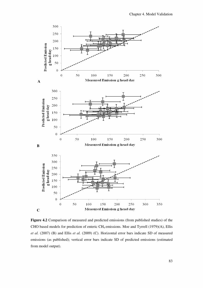
Chapter 4. Model Validation
83
A
B
C
Figure 4.2 Comparison of measured and predicted emissions (from published studies) of the
CHO based models for prediction of enteric CH4 emissions. Moe and Tyrrell (1979)(A), Ellis
et al. (2007) (B) and Ellis et al. (2009) (C). Horizontal error bars indicate SD of measured
emissions (as published); vertical error bars indicate SD of predicted emissions (estimated
from model output).

Chapter 4. Model Validation
84
4.5.2 Nitrogen Transactions
In contrast to enteric CH4 (where different predictive equations were assessed) the objective
of this section was to examine the accuracy of the current methodology in predicting N
transactions, and therefore how inaccuracy may influence predicted emissions. Methodologies
for prediction of N transactions are well established, and the current approach used in the
National Inventory Methodology (2006) is based on SCA (1990) and Freer et al. (1997)
(updated Freer et al. 2007).
Significant linear relationships (P<0.05) were determined between measured and predicted
values for all N transaction parameters (Table 4.12). Calculated concordance (Table 4.13)
demonstrates a strong relationship (0.94, correlation 0.94) between measured and predicted N
intake. In contrast to the results of the CH4 study (Figures 4.1 and 4.2) where variability of
measured/predicted emissions was considerably different; variability (as shown by the
horizontal and vertical error bars) is quite consistent between observed and predicted value
(Figures 4.3 and 4.4).
Table 4.12 Fitted Linear relationships between measured and predicted values for N excretion
parameters based on published studies.
Equation y-intercept Slope Significance SE Obs SE Pred
N Intake 17.6 0.88 P<0.001 18.7 4.3
N Retained 23.7 -0.20 P=0.034 3.0 0.7
N Excreted 29.7 0.91 P<0.001 7.09 1.6
N Urine -1.6 0.76 P=0.003 35.4 8.1
N Faecal 42.9 0.18 P=0.018 12.4 2.9
Despite the significant (P<0.05) relationship (Table 4.12) the model does not accurately
predict N retention particularly when measured values are high. Concordance (Table 4.13) is
considerably lower than observed with other N parameters (-0.08). Variability (Figure 4.4)
(Standard deviations, horizontal error bars) of measured values is considerably higher than
predicted values. Similarly to retained N, the accuracy of prediction of faecal N decreses with
increasing level of measured N in the faeces (Figure 4.4).
Urinary N is over predicted at lower levels and under estimated at higher levels of measured
urinary N. However, a significant (P<0.05) linear relationship between observed and
predicted was determined with a moderate concordance (0.53) and correlation (0.64).
Variability in measured values is considerably higher than predicted values. When excreted N

Chapter 4. Model Validation
85
is considered as a whole (faecal and urine N) the relationship improves, compared to when
they are considered as individual components Lin's concordance is also improved by
considering N excretion as a whole (0.94, compared with 0.53 for urinary N and 0.31 for
faecal N alone).
Table 4.13 Concordance and correlations between measured and predicted values for N
excretion based on published studies.
Equation Concordance Correlation Cb
N Intake 0.94 0.94 0.10
N Retained -0.08 -0.49 0.16
N Excretion 0.94 0.99 0.95
N Faecal 0.31 0.54 0.57
N Urine 0.53 0.64 0.83

Chapter 4. Model Validation
86
A
B
C
Figure 4.3 Comparison between measured and predicted values of N intake (A), N retention
(B) and Excretion of faecal N (C) based on published studies. Horizontal error bars indicate
SD of measured emissions (as published); vertical error bars indicate SD of predicted
emissions (estimated from model output). .

Chapter 4. Model Validation
87
A
B
C
Figure 4.4 Comparison between measured and predicted values of Urinary N excretion (A),
Total N excretion (B) and volatile NH3 (C) based on published studies. Horizontal error bars
indicate SD of measured emissions (as published); vertical error bars indicate SD of predicted
emissions (estimated from model output).

Chapter 4. Model Validation
88
4.5.3 Gaseous Nitrogen Emissions
For a number of these studies, particularly where emissions were measured using
micrometeorological methods, limited data was provided regarding the ration and intake (
McGinn et al. 2007, Todd et al. 2008, van Haarken et al. 2008). Further, intakes and live
weights (particularly for whole feedlot measurements) are likely to be an average of all
animals on the lot at the time of measurement. Where ration information was limited, N
intake as reported by the study was used as an input to the N Intake component of the model.
Concordance calculations (Table 4.15) demonstrate a low relationship (0.2827) between
observed and predicted NH3 emissions, although a significant (P<0.001) linear relationship
was fitted (Table 4.14). The model appears to be able to reasonably accurately predict
emissions at lower levels, but accuracy decreases as measured emissions increase, with
considerable underestimation at high levels of measured NH3 (Figure 4.4c). Variability was
not reported for estimates on an individual animal basis in the majority of studies utilised in
the validation process. These studies have primarily been micrometeorological work;
therefore per head emissions are extrapolated from whole site measurements of concentration,
variability is reported for measured concentrations, but not for values on a per head basis.
Table 4.14 Linear relationships between measured and predicted emissions of ammonia based
on published studies. There was insufficient data to evaluate a linear relationship between
measured and predicted values of nitrous oxide.
Equation y-intercept Slope Significance SE Obs SE Pred
NH3 28.3 0.21 P<0.001 6.7 2.0
Table 4.15 Concordance and correlations between measured and predicted emissions of
Nitrogenous gases
Equation Concordance Correlation Cb
NH3 0.28 0.94 0.30
N2O 0.00 1.00 0.00
Very limited data is available which links animal production characteristics to N2O emissions
from feedlot systems, resulting in inability to fit a linear relationship (Table 4.14) and very
low concordance (0.00, Table 4.14). However, a correlation of 1.0 was determined- related to
the low sample size. Although measurements have increased in this area the majority are

Chapter 4. Model Validation
89
undertaken using micrometeorological measurements, or using manure in chambers, which do
not always provide the details required for the modelling approach used here. Boadi et al.
(2004b) report N2O of 2.2 and 2.4 g/pen/day, equating to 0.15 g/head/day for the experimental
pens of 14 head. This is considerably lower than predicted emissions from this study (based
on the model described above) of 7.0 and 5.4 g/head/day. However, the study of Boadi et al.
(2004b) was conducted under conditions of very low temperatures; therefore they are unlikely
to represent the range of possible emissions. Modelled emissions based on the data provided
in the other studies used in the gas validation (only NH3 was reported) range from 3.3 to 10.7
g/head/day.
4.5.4 Sensitivity Testing
In most cases (excluding Boadi et al. 2004b) the estimates of intake (Table 4.9) using all
alternate methods are considerably greater than intakes recorded. Simple linear regression and
concordance calculations were used to examine the relationship between measured intake and
the alternative estimates of intake utilised in the methodology. Significant linear relationships
were determined between offered feed (measured intake) and intake predicted using Minson
and McDonald (1987) (P<0.01) and as a percentage of live weight (P<0.001) (Table 4.16)..
Lin’s concordance calculations (Table 4.17) showed the highest concordance between
measured intake and intake estimated as a percentage of live weight (0.30, correlation 0.90).
The equation of Minson and McDonald (1987) showed moderate correlation (0.53) with
measured intake values, but no concordance (0.00), whilst a set value based on class of cattle
had very low correlation and concordance (0.05 and 0.01) with measured intakes.
Despite the low concordance (Table 4.16) between measured and class-based-intake
estimates, utilising a class-based-intake actually improves the correlation between measured
and predicted CH4 emissions
Reported gross energy content (Table 4.17) varied from the set value (18.4 MJ GE/kg DM),
with a range of 17.8 to 19.5 MJ GE/kg DM measured in the examined studies. Weighted
average GE content was not concordant with the measured value (concordance -0.06,
correlation 0.13). Weighted average GE content was more variable (more difference between
min and max calculated values) for higher forage rations (e.g. backgrounding vs. finishing in
Beauchemin and McGinn (2005) and the 65:35 in Lovett et al. (2003)). This reflects the
variability in quality of the forage crops/ products. It also suggests that using a fixed value for
gross energy may not but suitable for all ration types, even within “feedlot” type rations.

Chapter 4. Model Validation
90
Concordance calculations demonstrate a high level of concordance between the emissions
predicted using the standard 18.4 MJ value for GE and the GE value reported by the studies
(0.99 tier II and 0.97; Blaxter and Clapperton 1965) and with the standard value and a
calculated weighted average based on ration composition (0.94 Tier II and 0.92; Blaxter and
Clapperton 1965). Strong correlations (>0.95) are also observed between emissions predicted
using the standard value, reported values and the calculated weighted average value for 18.4
(MJ GE/kg DM).
Table 4.16 Concordance and Correlations between measured CH4 output and CH4 output
predicted using measured intake, intake as a set value based on cattle class, intake calculated
based on the equation of (Minson and McDonald 1987), and intake as a percentage of live
weight. Predicted CH4 is based on five different equations.
Equation Intake Concordance Correlation
Tier II Measured 0.01 0.03
Class 0.13 0.43
Minson and McDonald -0.02 0.06
% Live weight -0.13 -0.23
Measured 0.05 0.02
Class 0.02 0.31
Minson and McDonald -0.01 -0.72
Blaxter and Clapperton (1965)
% Live weight -0.03 -0.31
Measured 0.19 0.52
Class 0.14 0.65
Minson and McDonald 0.11 0.47
Moe and Tyrrell (1979)
% Live weight 0.08 0.45
Ellis et al. (2007) Measured 0.09 0.14
Class 0.11 0.67
Minson and McDonald 0.04 0.13
% Live weight 0.00 0.01
Ellis et al. (2009) Measured -0.13 -0.21
Class -0.06 -0.15
Minson and McDonald -0.11 -0.28
% Live weight -0.10 -0.32

Chapter 4. Model Validation
91
Table 4.17 Reported and calculated* weighted average GE concentrations of rations used in the validation studies
Weighted Average GE Concentration
MJ GE/kg DM
Study Ration Reported Average Minimum Maximum
Corn Backgrounding 18.3 18.0 16.6 18.7
Barley Backgrounding 18.6 17.8 17.1 18.8
Corn Finishing 18.2 18.3 17.9 18.5 Beauchemin and McGinn (2005)
Barley Finishing 18.1 18.0 17.4 18.4
LF:G 17.8 17.5 17.0 18.0 Boadi et al. (2004b)
High F:G 18.8 15.2 14.6 15.9
LG 18.7 17.7 17.0 18.8 Beauchemin and McGinn (2006)
HG 18.7 18.2 17.7 18.8
Hegarty et al. (2007) - 17.8 16.8 16.2 17.2
65:35 19.5 17.8 15.0 19.5
40:60 18.8 17.3 15.4 18.6 Lovett et al. (2003)
10:90 17.9 18.1 17.2 18.8
*based on (Givens and Moss 1990)

Chapter 4. Model Validation
92
4.6 Discussion
4.6.1 Accuracy of the Models for Feedlot Systems
The accuracy of a number of the models used under Australian and International
methodologies for reporting emissions has been questioned (ALFA 2008), particularly in the
context of Carbon Trading and the Carbon Farming Initiative (Australian Government 2010a).
The National Inventory Methodology (AGO 2006) for enteric CH4 emissions from feedlot
cattle; Moe and Tyrell (1979) and the equation developed by Ellis et al. (2007) performed the
best, with a concordance of 0.26 and 0.29 respectively (although these correlations are still
poor). The approach of these equations is similar, basing potential CH4 emissions from a diet
on fermentative properties (fibre/ carbohydrate composition) rather than the total gross energy
and intake of the diet (as in Blaxter and Clapperton 1965 and IPCC Tier II). The factors used
are different between the two equations, but the most significant difference in terms of
approach is the inclusion of metabolisable energy intake as a factor in Ellis et al. (2007). Both
Moe and Tyrrell (1979) and Ellis et al. (2007) have the disadvantage of using parameters
which are not commonly measured in a commercial situation, for example Moe and Tyrrell
(1979) relies on estimated soluble residue, hemicellulose and cellulose, and Ellis et al. (2007)
on ADF and lignin. This is suggested by a number of sources as a source of error in the
prediction of CH4 emissions, particularly when tabulated values are required. Yan et al.
(2009) observed Ellis et al. (2007) to have a poor predictive ability for the range of diets
evaluated.
In general, the equations based on energy appeared to have poor predictive ability for feedlot
situations. The Tier II equation (concordance 0.14) appears to closely estimate emissions
when the grain content of the ration is high (greater than 90%), however in practice,
particularly in Australian feedlots, grain content is unlikely to be this high. This type of model
may have potential with the use of a diet specific Ym factor, rather than a set value for a type
of cattle (Kebreab et al. 2008). Estimates may also be improved by using offered feed in place
of a set value for intake. Both the energy based equations (Tier II and Blaxter and Clapperton
(1965)) are affected significantly by changing intake and GE estimation. These models are
unable to reflect differences related to ration composition (when a consistent group of cattle
are fed different rations), when intake is estimated on a class basis, or as a proportion of live
weight, and when a set value is used for GE. The National Inventory Methodology (AGO
2006) currently uses class-based-intake values, and a set GE, so it is likely that it would be
unable to identify feedlots which are using dietary changes to reduce CH4 emissions if these
equations were used.

Chapter 4. Model Validation
93
The trend for all the more complex approaches (excluding Tier II, 3% GEi) is for over
estimation of emissions. Over estimation (average) ranges from 33 g/head/day to 109
g/head/day, on average Tier II under estimates by 55 g/head/day. The primary reason for
inaccuracies in any of the methodologies is consistently identified as an effect of applying the
model on a range of data which is dissimilar to that on which the model was developed (Mills
et al. 2003; Wilkerson et al. 1995). For CH4 emissions, the most common source of this
variation is in ration components, although animal characteristics may also contribute. A
particular dietary parameter which is likely to result in overestimation of emissions using the
models evaluated is starch. Increasing starch in the ration alters rumen fermentation,
increasing propionate relative to acetate and decreasing hydrogen production (for the same
amount of consumed dry matter). As noted by Boadi et al. (2004a) fermentation of structural
CHO (cellulose, lignin etc) results in greater CH4 loss than the fermentation of soluble starch
and sugars. Structural CHO fermentation favours a decreased rate of passage and increased
production of acetate relative to propionate. Further, rapid fermentation of starchy grains (at
high intake levels) favours rapid rumen fermentation and increased propionate production.
Decreased rumen pH also restricts growth and activity of methanogens (Hegarty and Gerdes
1998). An example of the effect of alterations in CHO composition (ADF, NDF and starch)
with different grains is the differing CH4 emissions observed for corn and barley based diets
by Beauchemin and McGinn (2005). The starch content of barley grain was 54.5% and of
corn 66.7%. When used in a high concentrate (finishing) diet, emissions were less for a corn
based diet (9.2 g/kg DM) than barley based diet (13.1 g/kg DM).
Hindrichsen et al. (2004) tested a range of feed types varying in CHO properties (using
isonitrogenous and isocaloritic diets) in vitro and concluded that equations predicting CH4
from CHO fractions need to include starch and sugars as well as commonly evaluated
carbohydrate fractions. Although the equation of Moe and Tyrell (1979) includes a parameter
(soluble residue) which is primarily made up of starch, the proportion of soluble residue in the
diets utilised in the development of the model averaged 1.8 kg/day (.27 to 3.83 kg/day). As
previously discussed, inaccuracies in the majority of modelling approaches tend to arise when
they are applied to data outside the range on which they were developed (Mills et al. 2003).
For the majority of the studies utilised in this evaluation intake of soluble residue was greater
than 5 kg/day, which is significantly greater than those used in the development. This may
result in artificially high predicted values, where the impact of a high starch feed on
fermentation and microbial populations are not adequately represented by the models.
Further, these calculations of soluble residue are based on a standard value (according to the
National Inventory Methodology, AGO 2006). Soluble residue of concentrates is set at 0.19,

Chapter 4. Model Validation
94
grains 0.68 and roughages 0.21. However, as discussed in terms of GE, there can be
considerable variation between individual grains and roughages within these feed types.
Commonly used grains in Australian feedlot rations include barley and wheat in the south,
and sorghum in the north. Givens and Moss (1990) reports starch contents of 562 g/kg DM of
barley, 730 g/kg DM for sorghum and 674 g/kg DM for wheat, suggesting that a single value
for a feed type is unlikely to represent the range of soluble residue in a feed type.
Of key importance of assessing the impact that difference in specific dietary parameters is the
role of intake in influencing the amount of CH4 produced/ kg of component digested. Moe
and Tyrell (1979) report that CH4 production from carbohydrate depended more on the
amount fermented than the type of carbohydrate. At higher intakes >3.5 times maintenance
(intake requirement to maintain the animal in steady state) CH4 production was influenced
more by type of carbohydrate than at lower intakes. Moe and Tyrell (1979) determined at
intakes below 1.5 times maintenance requirement CH4 production is nearly as related to dry
matter intake or total digestible nutrients, but at intakes greater than 1.5 times intake
consideration of the amount of individual carbohydrate fractions digested. Relative intakes
calculated for the studies utilised in this evaluation (for enteric CH4) range from 0.5 to 1.05
(based on a standard reference weight of 660 kg), suggesting that dry matter intake or total
nutrients may be more highly correlated with CH4 emissions than carbohydrate fractions for
this range of data. However, these studies may not be entirely representative of an ad lib
feeding feedlot situation (especially where calorimetric methods may have affected intakes
and behaviour). Beauchemin and McGinn (2005) reports that measured CH4 emissions in
their study may underestimate those from commercial feedlot cattle due to a drop in intake
associated with chamber measurements.
The model for N transactions very accurately predicts N intake (R2 0.94, concordance 0.94).
This is not surprising, given this requires only intake and feed N concentration (the greatest
source of error here being intake estimation). Errors in the estimation of N intake occur at
higher levels, perhaps associated with N concentration in the feeds or variation in the
conversion factor between N and crude protein. In general, a factor of 6.25 is used to convert
N to crude protein, however represents an average value (similar to the 18.4 MJ/kg DM set as
the gross energy of feed). These higher N intake diets, such as Cole et al.(2005) and Adams et
al. (2004), contain byproduct feeds such as cottonseed meal (Cole et al. 2005) and
supplements containing urea, blood meal and feather meal (Adams et al. 2004). These
supplements are higher in non-protein N than traditional grains and forages, which are not
accounted for using a single factor for the N content of a feed. This is likely to have a flow on
effect to N excreted and therefore the balance between predicted and measured emissions.

Chapter 4. Model Validation
95
Nitrogen retention is poorly estimated by the model, (R2-0.49, concordance -0.01). This
model uses relative intake, relative size and live weight gain in prediction of retained N. The
errors in this estimation suggest problems with the standard reference weights, and
calculations of relative intake may not be suitable for feedlot type cattle. Similarly, the model
of CH4 production, produced by Blaxter and Clapperton (1965), which utilises a value of
relative intake has been found to overestimate emissions, compared with measured values.
Both relative size and intake are based on the concept of a standard reference weight.
Standard reference weight is defined as the weight of an animal when it reaches mature
skeletal size and has a condition score in the middle of the range (Freer et al. 2007). Feedlot
rations are designed to produce high rate of body growth and protein deposition, compared
with standard cattle growth, particularly on forage based diets. It has been observed by a
number of authors that N retention differs between ration types, with the primary effects
related to N intake, DMI and effects of live weight gain (Adams et al. 2004; Farran et al.
2006). However, specific effects have been reported with changes to forage type, grain types
and processing and method of protein feeding (e.g. phase feeding vs. constant protein level;
Cole et al. 2006). Addition of rumen modifiers to the diet is suggested to influence
propionate production and consequentially protein anabolism (Freer et al. 2007). The use of
these compounds (e.g. monensin) is increasingly common in feedlot systems and may result
in N transactions differing from predictions when its effects are not considered. Freer et al.
(2007) suggest alternations of the efficiency of growth factor to compensate for these changes
when modelling N retention.
Further, there are likely to be considerable difference between breeds in N retention. Moore et
al. (1975) determined significant differences in N retention between Angus, Hereford and
Brahman steers. B. Taurus breed steers exhibited higher N retention than B. Indicus steers fed
high energy rations, although these differences are less pronounced when lower energy
rations are fed. In addition to inaccuracies observed in the model here, utilising this approach
for a wider selection of Australian feedlot producers. Cattle populations in Northern feedlots
(depending on the season) can be predominantly B. Indicus type, while those in the Southern
feedlots are more commonly B. Taurus.
Validation of this component of the model is likely to be complicated by the methods used to
produce N retention in the published studies. Nitrogen retention in the majority of studies
used in the validation process is estimated based on animal live weights and live weight gains
using the procedures outlined by the (NRC 1996); the same approach used in the IPCC
guidelines. Effectively, this results in the results of one model being used to validate the

Chapter 4. Model Validation
96
results of a different model for N retention. This is likely to be a contributing factor to the
high level of variability observed in measured emissions.
The estimation of faecal N output is also fairly poor (R2 0.53, concordance 0.31). Greater
errors are observed at higher levels of measured faecal N excretion. Faecal N excretion is
estimated using digestibility, metabolisable energy, crude protein and feed intake. In the
general modelling approach a fixed value of 80% is used for the digestibility of the ration,
ME is also assumed based on this DMD (12 MJ ME/ kg MD). A fixed feed intake is
additionally incorporated for feedlot cattle. In the initial validation these fixed values were
used, some inaccuracy in the estimates of faecal N compared with measured values would
therefore be expected.
The accuracy of faecal N estimates decreases, with increasing levels of measured faecal N.
The higher measured values for faecal N result from the study of Adams et al. (2004). Steers
were kept in small feedlot pens for periods of 180 days during winter and 132 days during
summer. Total N intake and N excretion (measured from collection of manure and
measurements of changes in soil N) were determined for the whole period. Manure N in this
case was calculated based on the amount of material scraped from the pen, and the N content
of this material. It is likely that this over estimated manure N, the value of faecal N in this
study (Adams et al. 2004) ranged from (the equivalent of) 90 to 190 g/steer/day, compared
with 30 to 60 g/head/day in the other studies (Cole et al. 2003; Cole et al. 2006; Vasconcelos
et al. 2006). Despite the majority of urinary N being volatilised under most conditions there is
likely to have been some contribution from this source, particularly during the winter
measurement period. There may also have been a contribution of non volatile forms of N, for
example hair and scurf, feed waste and bedding material. The results of Cole et al. (2003) are
also inconsistent with other results, having considerably higher N intakes (average 218
g/head/day) and lower faecal N (average 30 g/day) compared with the other studies used in
the validation. It is well known that altering the concentration and ruminal degradability of
feeds alters N partitioning. It is possible that these diets, while having a higher level of N,
contained protein supplements which were quickly degradable (e.g. Urea), resulting in more
N being partitioned to urine (Cole et al. 2005).
In contrast to N retention and faecal N excretion urinary N excretion is estimated quite
accurately by the model (R2 0.99, concordance 0.94). The model predicts urinary N excretion
based on N intake, subtracting N retained and faecal N. Interestingly, despite the inaccuracy
in retained N and faecal N, urinary N is still estimated well. This suggests that the model is
able to estimate N “use” in the animal (if faecal N and retained N are considered together),

Chapter 4. Model Validation
97
but has errors when attempting to partition N between these areas. As urinary N is the major
pathway of N excretion, and the primary source of both volatile NH3 and emissions of N2O, it
is possible that the inaccuracy associated with faecal N excretion may not result in significant
alterations in predicted greenhouse gas emissions. This is confirmed by the examination of
total N excretion (Figure 4.4b). Considering total N excretion rather than the individual
components improves estimation based both on a regression between measured and modelled
and on concordance and correlations.
The use of a single factor to convert urine and faecal N to potential volatile NH3 and N2O is
the primary contributor to the inaccuracy associated with prediction of gaseous emissions.
Despite a reasonable prediction of urinary N, which is the major contributor to emissions of
both gases, NH3 emissions are quite significantly under estimated (Figure 4.4c), although
accuracy is better at lower measured values. Direct emissions of N2O were also significantly
over estimated by the model, although limited studies were able to be investigated. The major
issue which arises from attempting to predict gaseous N emissions from dietary components
and animal performance is the role which environmental conditions play in the emissions
process. As outlined in the literature review (Sections 2.4 to 2.6), moisture content, pH,
temperature, manure pack depth and organic matter content have a significant impact on
nitrification and denitrification, and volatilisation of NH3.
Emissions of NH3 vary between seasons, based on temperature and rainfall (contributing to
soil/ manure pack moisture). Todd et al. (2005) determined NH3 emissions of 55% of feed N
during summer, and only 27% of feed N during winter. They determined an emission factor
of 15 kg NH3/head/year, in contrast to the USEPA factors of 11 kg/head/day. Similarly
Klopfenstein and Erickson (2002) determined that 60-70% of feed N was lost as NH3 in
summer, and 40% during winter. Todd et al. (2005) report that NH3 emissions were greatest
in hot dry weather, and precipitation suppressed NH3 emissions. Denmead et al. (2008)
determined emission rates of 69 g NH3-N/animal/day for a temperate Australian site and 24 g
NH3-N/animal/day for a tropical Australian site (during winter). They attributed this to
differences in surface wetness, which was higher at the temperate site and therefore allowed
increased volatilisation of NH3; this contrasts with the observation of Todd et al. (2005). Loh
et al. (2008) report summer emissions from the same sites during summer, equal to 170 g
NH3-N/head/day (tropical) and 117 g NH3-N/head/day (temperate). In a discussion of these
results, Denmead et al. (2008) also cite surface wetness as the major factor influencing
emission rate.

Chapter 4. Model Validation
98
Although there is insufficient data to estimate concordance between measure and predicted
N2O emissions; predicted N2O emissions from these studies ranged between 3.3 and 10.7
g/head/day. Denmead et al. (2008) report emissions of 1.1 and 1.8 g N2O-N/head/day from
Australian feedlots, whilst Boadi et al. (2004b) determined N2O emissions equivalent to 0.16
g/head/day (using chamber incubations), which was approximately 50% of that estimated
using IPCC calculations (the same coefficient used in the methodology examined here).
Further examination of the source of the IPCC emission factor for dry lot manure
management reveals a number of issues in the potential application of the source study to a
feedlot situation. According to the IPCC methodology- the default emission factor of 0.02 for
N2O emissions was developed based on the work of Kulling et al. (2003) and consultation
with the expert committee. The study of Kulling et al. (2003) was focussed on emissions from
dairy manure comparing three management systems (slurry, liquid and farmyard manure) and
two rations types (hay or grass based). It can be assumed that the farmyard manure
management system was considered similar to feedlot, as this was the driest and most
compacted material. However, this material was amended with straw, in order to replicate the
bedding system used in Switzerland. The types of rations used, resultant changes in manure
composition compared with a feedlot suggest that emission factors developed for this work
are unlikely to be entirely applicable to dry lot management systems. However, Kulling et al.
(2003) reports emissions of N2O between 1.7 and 2.8 g/head/day, very similar to those
measured in an Australian feedlot (Denmead et al. 2008).
4.6.2 Sensitivity of Models
Changing intake prediction influences the models differently. The simplest model, Tier II
(IPCC 2006), which was shown by the validation process to be mid range in terms of
concordance between measured and modelled emissions, is significantly affected by changing
intake. When cattle are fed different rations, we would expect that a higher grain/ more
digestible ration to result in lower CH4 emissions, which is reflected in the measured values.
When a class based or % live weight intakes are applied to a consistent group of cattle, the
Tier II model does not reflect any differences in ration composition (this is associated with the
use of a set factor for GE. A similar issue is associated with the Blaxter and Clapperton
(1965) equation, which uses a set value for GE and digestibility, with the differences in
emissions therefore resulting from intake (through the relative intake parameter). The
carbohydrate equations, in contrast, are able to reflect differences in ration composition, even
when intake is estimated using a fixed value for the class or live weight of the animal. If these
equations were to be utilised for inventory purposes it would enable the reduction in enteric
emissions associated with diet type to be accounted for, however, an assessment of intake

Chapter 4. Model Validation
99
values set for a specific class may need to be undertaken, given the overestimation of intake
for all equations examined here.
As the National Inventory Methodology (AGO 2006) currently uses a fixed value for the class
of feedlot cattle (referred to in this discussion as the ‘methodology’ estimate of intake) the
higher estimate is likely to result in over estimation of emissions, compounding the issues
with over estimation which are already observed with most models of enteric CH4. As the
most concordant estimate of intake was the equation of Minson and McDonald (1987), it
would be assumed that predicting intake using this equation would improve the estimate of
CH4 from the model, relative to the fixed values from the methodology and as a % of live
weight. For inventory purposes, it would be impractical to record intake of individual animals
on a daily basis, or even over the time spent on feed, for the calculation of emissions. Even
calculating based on growth is impractical as measurements such as weight are not commonly
calculated on an individual basis in the feedlot (as well offered feed is on a per pen basis).
However, these results suggest that improved estimates of intake are required; if a set value
(for intake) is going to be used in a Tier II approach.
4.6.3 Further Considerations
When evaluating the results of the validation process, the difference in standard deviation (as
represented by the error bars) between measured and modelled emissions is a concern. For
many of the models (e.g. Tier II, Moe and Tyrell 1979, Ellis et al. 2007 and Ellis et al. 2009)
modelled emissions are significantly less variable than measured emissions. For Tier II, this is
likely to be related to the parameters set by the model, feed gross energy is set at 18.4 MJ GE/
kg DM, and CH4 as a percent of gross energy at 3%. As discussed individual feed gross
energy can range from 14.7 MJ/ kg DM to 39.3 MJ/ kg DM (Givens and Moss 1990), and the
reported values for the validation study rations ranged from 17.8 to 19.5 MJ GE/ kg DM.
Although a high level of concordance was observed between modelled emissions using a
variety of different GE values using set values for these parameters would significantly
reduce the variation associated with modelled emissions. A single figure of 3% does not,
therefore, demonstrate the natural variation in emissions, although it provides a reasonable
overall estimate for higher concentrate rations.
The reason for the lower variation in the other equations, which are feed/ carbohydrate based,
is likely to be similar. These equations all use ration contents of factors such as hemicellulose,
cellulose, soluble residue etc, and calculate potential emissions from these fractions.
However, the accuracy of these estimates can be significantly affected by the method used in
determination, and even by the feed and forage type. Hemicellulose and forage cellulose, key

Chapter 4. Model Validation
100
parameters in both Moe and Tyrell (1979) and Ellis et al. (2009) is often estimated using NDF
and ADF content of feeds, or using ADF minus sulphuric acid lignin (Hans-Joachim 1997).
Hemicellulose, when estimated as NDF-ADF is often overestimated by the presence of non
extracted proteins in the NDF (Hans-Joachim 1997). For this to provide a reasonable estimate
of hemicellulose, NDF and ADF need to be sequentially determined. The original method of
determination of NDF and ADF (Van Soest et al. 1991) has been modified considerably since
its conception and therefore equations developed based on the original method (e.g. Moe and
Tyrell 1979) may be inaccurate when values determined using the modified method are
utilised in the calculations (Hao et al. 2001a).
Ellis et al. (2007) uses ADF and lignin; as reported by Hans-Joachim (1997) the measurement
of lignin is complicated due to variable methods (at this point there was no definitive
reference method). The most common method is acid detergent lignin, however evidence
suggests that lignin is underestimated using this method (Hans-Joachim 1997). However,
Hindrichsen et al. (2004) examined a variety of methods for estimating cellulose,
hemicelluloses and lignin and determined high correlations between methods for cellulose
(0.99) and lignin (0.93), but low correlation for hemicellulose (0.44). They attribute this to
high amounts of soluble hemicellulose in some feeds, which was washed out during NDF
analysis. However, this highlights the impact that measurement method may have on
measured parameters and consequentially the potential for errors in prediction based on this
data.
Further, the parameters used in this equation (soluble residue, cellulose and hemicelluloses)
are not commonly measured in commercial feed testing, and are therefore estimated based on
fixed values in the methodology. There can be a significant variation in the estimation of
these parameters, depending on the feed type. An examination of the data used in the
development of the model demonstrates the range in the contents of soluble residue,
hemicellulose and cellulose with the rations used. Soluble residue varied from 18.1 to 54.1%,
hemicellulose from 7.1 to 28.2% and cellulose from 8.5 to 34.3% (Moe and Tyrrell 1979).
As discussed by Yan et al. (2000) most of the earliest developed equations were based on
animals offered dry or high DM forages, this may not reflect the lower DM silages used in
feedlot rations. Fermentation processes in silages which result in low concentrations of water
soluble CHO, and high levels of fermentation products (e.g. VFA) which result in differences
in rumen processes (Yan et al. 2000), reducing the ability of the model to reflect rumen
processes, hydrogen production and therefore CH4 emissions.

Chapter 4. Model Validation
101
Measurement method can have a significant impact on reported emissions, and therefore on
the perceived accuracy of models. Boadi et al. (2004b) measured CO2 and CH4 emissions
using both the SF6 tracer technique and calorimetric methods; although animals and rations
remained constant a significant difference was observed in CO2 output. Similarly, Grainger et
al. (2007) compared the chamber and SF6 measurements of CH4 and determined significant
differences in measured emissions of CH4, which could not be entirely accounted for by hind
gut CH4 production. Yan et al. (2009) suggest that the poor predictive ability of some models
(e.g. Ellis et al. (2007)) may be related to some of the data used in the development being
measured using the SF6 techniques, which does not measure emissions from the hindgut,
therefore under estimating emissions. In contrast Ellis et al. (2009) did not find measurement
method to have a significant effect on CH4 output, when CH4 was expressed as MJ/day, or as
% of gross energy.
Although the National Inventory Methodology (AGO 2006) for estimating manure CH4 takes
into consideration differences between environmental conditions between tropical and
temperate regions of the country (CH4 conversion factors of 5% and 1.5% are used for
tropical and subtropical areas respectively) this is not followed through to either volatile NH3
or N2O . A number of studies have determined significantly different NH3 emissions between
seasons and feedlot sites. This suggests that at a minimum, modifications need to be made to
the emission factor used in order to more accurately represent NH3 volatilisation. The current
emission factor used in the inventory is 30 % of excreted N, or 0.3 kg/kg excreted N. This is
considerably lower than calculated emission factors of 0.6 (Denmead et al. 2008), 0.6-0.7
(Bierman et al. 1999) and 0.9 (Loh et al. 2008). As evidenced by the validation study, the
emission factor (or fraction of volatile N) is too low under some circumstances, and does not
account for differences in environmental conditions which have a significantly impact on
emissions.
4.7 Conclusion
Although there has been recent research into emissions from Australian beef and dairy
systems, including feedlots (Alford et al. 2006; Charmley et al. 2008; Chen et al. 2009;
Denmead et al. 2008; Hegarty et al. 2007; Loh et al. 2008; McGinn et al. 2008), the accuracy
of the current National Inventory Methodology (2006) for the estimation of Greenhouse
sources and sinks (as it applies to feedlot systems) has not been formally examined under
commercial conditions.
This validation exercise suggests that for the most accurate estimation of emissions from
feedlot systems, and the ability to distinguish between diet types, a methodology based on

Chapter 4. Model Validation
102
dietary composition is required. The National Inventory Methodology (AGO 2006) equation;
Moe and Tyrell (1979), has the benefit of utilising this approach, and along with Ellis et al.
(2007) provide the best estimates of CH4 emissions. However, the IPCC Tier II approach
merits further investigation.
Despite errors in estimating retained N and faecal N, urinary N and total N excretion are
estimated reasonably well by the model. However, this is not translated into accurate
estimation of emissions of NH3. Insufficient data was available to determine accuracy of
models for N2O, however predicted emissions from the studies utilised were higher than the
range of measured emissions from beef cattle. Errors in estimating the emissions of NH3
using this methodology are likely to result from the use of a single “emission factor” which
does not represent emission potential under all environmental conditions.

Chapter 5. Model Application
103
Chapter 5. Measured Emissions and Application of a Model
for Estimation of Greenhouse Gas Emissions from
Australian Beef Feedlots
5.1 Introduction
Under the United Nations Framework Convention on Climate Change (UNFCCC) the
Australian government is obligated to produce inventories of annual emissions of greenhouse
gases produced under agricultural (and other industrial) activities. The inventories are
produced based on a methodology developed by The National Greenhouse Gas Inventory
Committee (NGGIC), published by the Australian Greenhouse Office (AGO) in accordance
with IPCC guidelines (IPCC 2006). Globally, there is a lack of data available on baseline
emissions from cattle breeds (particularly tropical (B. Indicus) breeds) and life stages
representative of the feedlot industry (Stackhouse et al. 2011), although there has been
considerable focus on greenhouse gas emissions from Canadian and Northern American
feedlot cattle, in more recent years (Beauchemin and McGinn 2005; Beauchemin and McGinn
2006; Boadi et al. 2004b; Kebreab et al. 2006; McGinn et al. 2009; van Haarlem et al. 2008).
Locally, concerns have been expressed by industry bodies regarding the accuracy of this
method (ALFA 2008) and about the impact of errors in emissions estimates under a carbon
constrained future on profitability and industry sustainability. There has also been limited
validation of models commonly used for predicting emissions from feedlot cattle, particularly
with respiration chamber experiments (Kebreab et al. 2006; Stackhouse et al. 2011).
Meat and Livestock Australia studies suggest that the feedlots are already paying
$2.35/standard cattle unit on environmental management, without the further cost of
managing a carbon reduction/ trading scheme (Monni et al. 2007). Accurate estimates are
important under all prospective applications of a carbon constrained economy, in order for
mitigation options to be accounted for, and to reduce the economic impact of a direct Carbon
Tax.
The equations developed to predict emissions of CH4 are based on measurements conducted
in order to examine the metabolisable energy partition from feed GE (GE minus loss of
energy in faeces, urine and gases). Blaxter and Clapperton (1965) produced their equation
(which now forms the basis of a number of national inventories) in order to predict losses of
energy as CH4 by cattle and sheep from knowledge of feed composition and intake. Similarly,

Chapter 5. Model Application
104
Moe and Tyrrell (1979) assert the need for direct measurements of CH4 production, or
adequate means of estimating emissions. Although the current focus on CH4 is as a
greenhouse gas, CH4 emitted from a system additionally represents a loss of energy (as
reflected by the development of the original equations). In theory, reducing loss of CH4
energy could provide increased energy for growth. However, the emission of both CH4 and
nitrogenous gas can be considered an inefficiency of the system, the reduction of which
should have benefits for both productivity and economic performance. Accurate estimates
may provide a tool for managers to improve efficiency of production as well as advising
decisions on mitigation of emissions.
Chapter 4 evaluated a range of methodologies for the estimation of enteric CH4 emissions, as
well as examining the current prescribed model for predicting emissions of NH3 and N2O
from livestock manure. Utilising the results of published studies based on feedlot cattle from
(predominantly) the Northern hemisphere. The current Australian empirical equation for
feedlots, Moe and Tyrell (1979), was observed to have a relatively low (0. 25) concordance
between observed and predicted enteric CH4 emissions. However, utilising an equation based
on nutrient fractions improved predictive ability compared with equations based on energy
consumption (concordance increase from 0.10 and 0.13 for the energy based equations to 0.25
and 0.28 for the nutrient fraction based rations). The results of Chapter 4 suggest issues with
overestimation exist in the current methodology for feedlot cattle; however, as discussed by
Mills et al. (2003) validation of a model for one location does not guarantee accuracy under
different conditions, therefore the model needs to be tested under Australian commercial
conditions.
Based on the results of Chapter 4, the two models for enteric CH4 with the most potential in
terms of accuracy of prediction were those based on carbohydrate fractions, Moe and Tyrell
(1979) and Ellis et al., (2007). However, the IPCC Tier II model (energetic based) shows
potential particularly for higher grain rations and was therefore considered for potential
application. The application of these models to data collected in Australian feedlots and
measurements undertaken using micrometeorological methods will be discussed in this
Chapter. Detailed climatic and animal production information was additionally collected, and
reasons for differences between sites and seasons in measured CH4, NH3 and N2O emissions
will be evaluated.
An evaluation (Chapter 4) of the N partitioning and gaseous emissions estimated based on the
current National Inventory Methodology (AGO 2006) suggested that while N excretion as a
whole (combined urine and faecal N) is predicted relatively well (concordance 0.94, R2 0.85)

Chapter 5. Model Application
105
individual components of N partitioning in the animal (in particular faecal and retained N) are
poorly estimated. Although this gives confidence that the amount of N being excreted by
feedlot animals is estimated accurately, the evaluation process suggests that the use of fixed
values to covert this figure to emissions of nitrogenous gases results in inaccuracies
(concordance 0.27 for NH3) related to the impact of environmental conditions. The 30% of
excreted N figure is accurate at the lower range of measured emissions, but accuracy
decreases as measured emissions increase.
5.1 Research Questions
This section aimed to build on the previous chapter and address the following questions
utilising data and measured emissions from two commercial Australian feedlots.
1. Is the current Australian National Inventory Methodology for estimating greenhouse
sources and sinks accurate in predicting emissions of CH4, N2O and NH3 from
feedlots?
2. Are equations based on energy or carbohydrate more accurate in estimating CH4
emissions?
3. What is the impact of using a single emissions factor in the model to predict NH3 and
N2O?
4. Does introducing equations developed based on beef cattle data improve accuracy of
estimates compared to measured values of CH4 emissions compared with the current
approaches?
5. Which factors contribute to differences in measured emissions at each site and
between seasons
5.2 Methodology
Full details of the feedlots studied can be found in the General Methodology Section 3.1.
Briefly, micrometeorological measurements of greenhouse gas emissions were undertaken at
two Australian feedlots during two seasons over two years. Details of the
micrometeorological measurement methods can be found in the General Methodology,
Section 3.2.
The objective of this modelling approach was to utilise data available from commercial
feedlots. Therefore during the measurement campaigns information was collected from the
feedlot operators in the form of bunk sheets, lot sheets, rations and daily feed amounts. This
information was collected for a minimum of five days for each 14 day measurement

Chapter 5. Model Application
106
campaign. Information collected included number of head (cattle) in each pen, animal sex,
estimated weight on entry and at the report date, days on feed, cattle class, rations and
amounts of feed offered. This information is easily available using feedlot management
software, and is collected and maintained by commercial feedlots on a routine basis.
Therefore the ability to use this type of data to estimate emissions will enable estimates to be
made simply for an individual operation.
The collected data was utilised as input for the model outlined in the general methodology.
Three of the described equations for estimation of enteric CH4 (Ellis et al. 2007; Moe and
Tyrrell 1979 and IPCC Tier II) were utilised in the application of the model to this data, based
on the results of Chapter 4.
5.2.1 Assumptions
Standardised inputs (Table 5.1) were utilised for the model (where appropriate) for both
feedlot sites, and where these values are specified by the National Inventory Methodology
(AGO 2006). Standard values are commonly used for feed composition where factors are not
commonly measured, such as GE (energy content of ruminant rations is more commonly
expressed as ME or net energy NE), soluble residue, cellulose and hemicellulose. Where
required dietary parameters (e.g. lignin) were not given as standard values this information
was taken from the appropriate feed type as reported by Givens and Moss (1990).
Although more detailed information regarding intakes, live weight gain (forecast) and current
weights was available from the feedlot operators than would be used in producing inventory
calculations animal class was required to be translated from the denominator used by the
operators to a numerical representative of class. This was based on information provided by
the feedlot management.
Inventory guidelines (AGO 2006) suggest intakes (kgDM/head) of 2 to 2.4% of live weight
(dependent on animal class). Where intake/ offered feed data provided by the feedlot
operators indicated intakes of greater than 3% of live weight these values were replaced by
intakes predicted based on percentage live weight. Intakes higher than physically possible
(due to large amounts of offered feed on a given day) result in artificially inflated emissions
predictions, which are unlikely to occur in practice. Further, where no offered feed or very
low offered feed (less than one kgDM/head) were reported these values were replaced by
intake as a percentage of live weight. Intake in ruminant animals is limited by physical
capacity of the rumen. It is unlikely that feedlot cattle will consume feed (even offered ad lib)
greater than 3% of live weight. Holt et al. (2004) formulated ad lib grain rations for feedlot

Chapter 5. Model Application
107
cattle (starting at 324 kg LWT) at 2.6% LWT. Similarly, Hicks et al. (1990) measured intakes
of feedlot cattle arriving in a feed yard, measuring DM intake weekly from entry to 150 days
on feed, DMI as a percentage of live weight ranged from 2.7% at the start of feeding, to 1.6%
during the finishing period. Maximum intakes were observed during the middle of the feeding
period (approximately days 40 to 80), however based on growth rates provided DMI during
this period was close to 2.5% LWT. These estimates support those reported in the National
Inventory Methodology (AGO 2006) and by van Sliedregt et al. (2000).
Table 5.1 Standardised values utilised in the prediction of greenhouse gas emissions from
beef feedlot cattle.
Parameter Set Value
Standard Reference Weight kg 660
GE content of rations MJ/ kg DM 18.4
Digestibility of rations % 80
N2O Emission Factor 0.02
NH3 Proportion of Excreted N 0.3
Manure CH4 conversion factor- temperate 0.015
Manure CH4 conversion factor- hot 0.05
Soluble Residue* g/kg DM
Grains
Concentrates
Forages
0.68
0.19
0.21
Cellulose* g/kg DM
Grains
Concentrates
Forages
0.07
0.19
0.31
Hemi- Cellulose* g/kg DM
Grains
Concentrates
Forages
0.31
0.31
0.21
* Based on AFIC (1987)
Removing offered feed amounts larger than what can physically be consumed by a feedlot
animal removes artificially inflated emissions- which do not represent the biology of the
system. Additionally, feedlot cattle are managed to produce maximum growth, therefore the
offering feed of less than 1 kg/head, less than 0.2% LWT for a 500 kg steer, would not be
Chapter 5. Model Application
108
indicative of the amount of feed offered (as reported in “bunk” or “lot” sheets) to support
growth in these animals. It is likely that small amounts of feed were offered in these cases to
provide a small top up from larger amounts offered in the previous days and do not reflect the
actual amount consumed by these animals. Intake as a percentage of live weight was found in
the previous Chapter (4) to have a moderate concordance (compared with a set value for live
weight/class and the equation of Minson and McDonald (1987)); however this was selected
for simplicity.
Metabolisable energy (ME) content can be estimated based on diet digestibility, with 80%
digestibility equating to approximately 12 MJ ME/kg DM. Overall digestibility of the rations
used in the feedlots was not available in the rations composition provided, therefore the
standard value of 80% was used, however ME provided in the ration formulation was used in
the calculations where required.
5.2.2 Emissions from Manure
Measurements using micrometeorological methods do not enable emissions of CH4 to be
partitioned between animals, or between enteric and manure pad emissions. Modelled
estimates and results of Boadi et al (2004b) suggest that CH4 emissions from the manure pad
equate to less than 2 g/head/day, therefore emissions measured using micrometeorological
methods can been attributed almost entirely to enteric emissions. For the purpose of this
evaluation CH4 measured using micrometeorological methods was assumed to reflect
primarily enteric CH4, and used in analysis as such (manure excluded from estimated CH4).
The primary source of NH3 and N2O in the feedlot is the pen/ manure surface and the effluent
management system. The software used in calculating emissions using wind statistics and
concentration measurements accounts for the effluent ponds as a source and discounts periods
where wind statistics indicate the measured concentration is derived primarily from this area.
There is some evidence of N2O production in the rumen (depending on dietary composition;
Kaspar and Tiedje 1981); however this is unlikely to make a significant contribution of total
measured emissions. There is also a possibility of NH3 and N2O production through
fermentation and microbial reactions in feedstuffs, particularly if these become wet (through
rainfall) or remain sitting in the feed bunk for long periods. Where nitrite or NO3 is present in
grass N2O can be formed during ensiling, however a less acidic (low soluble carbohydrate)
silage will show increased conversion of NO3 to ammonium (NH4; Hill 1999). The formation
of anaerobic pockets in distributed feeds may result in further production of N2O or NOx;
although this is unlikely to be as significant a source as manure decomposition. An emission

Chapter 5. Model Application
109
factor for N2O release from grass silage of 15g N2O-N/ kg NO3-N (Hill 1999), however this
represents the ensiling process, not post ensiling fermentation. For the purposes of this
analysis measured emissions of NH3 and N2O are considered to be derived from the manure
pad.
5.2.3 Statistical Analysis
Details of the bLS approach used in the measurement and calculation of fluxes/emissions in
g/head/day are described in the general methodology (Chapter 3). Average emissions
estimated for each of the three gases (CH4, N2O and NH3) was calculated for each day of data
collected from each measurement campaign. Average estimates reflect the average over the
useable data collected for the entire measurement campaign. Standard deviations reflect the
variation over the entire measurement campaign. Linear regression (Genstat v. 11 VSN
international) was used to examine relationships between measured and predicted emissions.
Significance represents the fit of a linear equation to the data, the probability that correlation
is greater than 0. Lin’s concordance (Genstat v. 11 VSN international) was used to measure
how well the modelled data reproduces the original data set (Lin 1989; Lin 2000). The
concordance coefficient is calculated using a simple Pearson’s correlation coefficient
(reported in text as the correlation between the variables) and the slope and origin of the line,
known as Cb.
5.2.4 Input Data
Model input was derived from information collected from feedlot operators during the
measurement campaigns (Table 3.1). An objective of this approach was to utilise information
readily available from commercial feedlots, therefore data was collected from feedlot
operators in the form of standard outputs from management software. The Northern feedlot
had a capacity of 17,000 and was operating between maximum capacity and approximately
1/3 capacity during the four campaigns. The Southern feedlot had a maximum capacity of
20,000 head, and was operating between 12,000 and 18,000 head during the four
measurement campaigns. Total number of head was higher in all campaigns at the Southern
Site than at the Northern Site.
In contrast to experimental data, where live weight, live weight gain and feed intakes are
recorded for individual animals, the information provided by the feedlot operators is on a pen
or “lot” (cattle group) basis. Live weight is estimated for a group of cattle on arrival (based on
the weight of the consignment of cattle (in the transport vehicle) and used to determine an
average start weight. Live weight is then computed from number of days on feed, and

Chapter 5. Model Application
110
estimated live weight gain (for class, offered feed amount and ration type); very few cattle are
weighed individually. Average live weight (Table 5.2) was higher and more variable at the
Northern Site. Estimated daily live weight gain and offered feed were consistently higher at
the Northern Site. This is related to the differing market targets of the two sites, which long
fed export cattle being the primary output of the Northern Site compared with shorter fed
domestic class cattle at the Southern Site.
Basic environmental conditions (Table 5.3) were measured at each site (including detailed
wind statistics). Temperatures showed typical seasonal variations at both sites. However,
there was more variation between summer and winter minimum temperatures at the Southern
Site than the Northern Site. Rainfall was substantially higher during the final two
measurement campaigns at the Northern Site, than for the remainder of the measurement
periods Mean wind speed (km/h) also tended to be higher in summer at both sites, with
consistently higher “gust” speed during summers at the Northern site. Overall average wind
speed was higher at the Northern site.
.

Chapter 5. Model Application
111
Table 5.2 Feedlot stock characteristics (mean and SD) averaged over the duration of eight measurement campaigns. Data was collected from feedlot
operators in the form of standard management software outputs.
Campaign Number of
Head
Live weight*
Kg
Estimated Live weight gain
kg/day
Offered Feed
kgDM/head/day
Southern Summer 2008 12863 455 ± 68.2 1.3 ± 0.33 9.7 ± 1.89
Southern Winter 2007 13107 441 ± 91.5 1.3 ± 0.35 9.4 ± 1.76
Southern Summer 2007 16593 519 ± 101.0 1.4 ± 0.37 10.1 ± 1.96
Southern Winter 2006 18137 492 ± 93.5 1.3 ± 0.38 10.1 ± 1.64
Northern Summer 2008 6167 756 ± 132.8 1.6 ± 0.46 11.9 ± 2.04
Northern Winter 2007 10554 530 ± 117.8 1.8 ± 0.23 11.3 ± 1.95
Northern Summer 2007 13747 562 ± 118.3 1.8 ± 1.00 10.4 ± 1.81
Northern Winter 2006 16655 546 ± 214.5 1.9 ± 1.62 10.3 ± 2.33
*Current live weight is estimated based on entry weight, days on feed and estimated live weight gain (based on class, ration and feed offered).

Chapter 5. Model Application
112
Table 5.3 Environmental conditions at two feedlot sites (northern and southern Australia) during eight measurement campaigns (covering summer
and winter)
Average Daily
Temperature
(°C)
Rainfall
(mm)
Average Daily
Wind Speed
(km/h)
Average Daily
Relative Humidity
(%)
Min Max Total Mean Gust Min Max
Southern Summer 2008 12.0 26.7 0.2 10.8 37.0 17.7 68.2
Southern Winter 2007 4.7 19.7 4.4 4.2 32.7 63.1 90.5
Southern Summer 2007 19.1 34.4 7.4 9.2 19.9 23.5 71.8
Southern Winter 2006 3.3 15.2 2.0 6.7 29.6 49.3 89.8
Northern Summer 2008 19.0 29.7 61.4 11.8 32.5 48.1 71.3
Northern Winter 2007 10.4 18.9 23.6 7.4 17.3 48.5 83.7
Northern Summer 2007 17.9 31.8 0.0 12.6 45.5 24.6 77.6
Northern Winter 2006 12.3 25.3 4.4 8.1 18.0 31.8 70.4
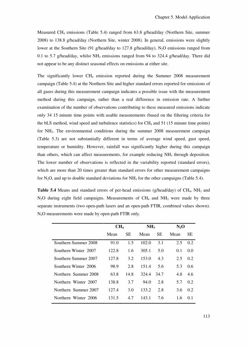
Chapter 5. Model Application
113
Measured CH4 emissions (Table 5.4) ranged from 63.8 g/head/day (Northern Site, summer
2008) to 138.8 g/head/day (Northern Site, winter 2008). In general, emissions were slightly
lower at the Southern Site (91 g/head/day to 127.8 g/head/day), N2O emissions ranged from
0.1 to 5.7 g/head/day, whilst NH3 emissions ranged from 94 to 324.4 g/head/day. There did
not appear to be any distinct seasonal effects on emissions at either site.
The significantly lower CH4 emission reported during the Summer 2008 measurement
campaign (Table 5.4) at the Northern Site and higher standard errors reported for emissions of
all gases during this measurement campaign indicates a possible issue with the measurement
method during this campaign, rather than a real difference in emission rate. A further
examination of the number of observations contributing to these measured emissions indicate
only 34 15 minute time points with usable measurements (based on the filtering criteria for
the bLS method, wind speed and turbulence statistics) for CH4 and 51 (15 minute time points)
for NH3. The environmental conditions during the summer 2008 measurement campaign
(Table 5.3) are not substantially different in terms of average wind speed, gust speed,
temperature or humidity. However, rainfall was significantly higher during this campaign
than others, which can affect measurements, for example reducing NH3 through deposition.
The lower number of observations is reflected in the variability reported (standard errors),
which are more than 20 times greater than standard errors for other measurement campaigns
for N2O, and up to double standard deviations for NH3 for the other campaigns (Table 5.4).
Table 5.4 Means and standard errors of per-head emissions (g/head/day) of CH4, NH3 and
N2O during eight field campaigns. Measurements of CH4 and NH3 were made by three
separate instruments (two open-path lasers and an open-path FTIR, combined values shown).
N2O measurements were made by open-path FTIR only.
CH4 NH3 N2O
Mean SE Mean SE Mean SE
Southern Summer 2008 91.0 1.5 102.0 3.1 2.5 0.2
Southern Winter 2007 122.8 1.6 305.1 5.0 0.1 0.0
Southern Summer 2007 127.8 3.2 153.0 4.3 2.5 0.2
Southern Winter 2006 98.9 2.8 151.4 5.6 5.3 0.6
Northern Summer 2008 63.8 14.8 324.4 34.7 4.8 4.6
Northern Winter 2007 138.8 3.7 94.0 2.8 5.7 0.2
Northern Summer 2007 127.4 3.0 133.2 2.8 3.6 0.2
Northern Winter 2006 131.5 4.7 143.1 7.6 1.6 0.1

Chapter 5. Model Application
114
A detailed investigation of animal behaviour and interactions with emissions is undertaken in
Chapter 6. Diurnal emissions patterns observed during this study demonstrate peaks in
emissions of NH3 at around midday. CH4 emissions tended to be lowest during the late
morning and early afternoon, corresponding with feeding and high temperatures (decreasing
rumination). However, for both NH3 and CH4 measured during this campaign (Northern
Summer 2008) the periods with measured emissions occurred primarily between 9 am and 4
pm, capturing the peak emissions from NH3, and lows in emission of CH4. This is likely to
lead to higher calculated emissions for NH3, and lower for CH4. For these reasons, the
measured emissions from the Northern Summer 2008 campaign were not utilised in this
evaluation.
Detailed ration information (Table 5.5) was also recorded at each site during each
measurement campaign. At the Southern Site, barley and wheat are the most commonly used
grains, whilst sorghum forms the basis of the Northern Site rations. Both sites use silages
(whole crop sorghum silage at the Northern Site and grass silage at the Southern Site) and dry
forages (hay and straw) and some by-product feeds (including bread crumbs). There is a
greater use of cotton seed and processed products of cotton seed (meal and hulls) at the
Northern Site. Proportion of grain tends to be higher on average at the Northern Site (61 to
71% at the Southern Site, compared with 71 to 81% at the Northern Site). Grain concentration
tended to be more variable at the Southern Site (particularly during 2007) than the Northern
Site. The Southern Site also reported the use of a hay only ration for newly arrived cattle
transitioning to the feedlot.
Excluding the hay only ration (which is fed to a very limited number of cattle over short time
frames) average DM (Table 4.6) was slightly higher (73% cf. 70%) at the Southern Site, as
was CP % (14.0 % cf. 13.6%, ME (MJ/ kg DM, 12.2 compared with 12.0) and average fat
content (kg/kg DM). At both sites, fat (recycled oil or vegetable oil) was included in a limited
number of rations (approximately two at each site during each campaign).

Chapter 5. Model Application
115
Table 5.5 Major ration Ingredients and proportions of grain at two feedlots sites over 8 measurement campaigns
Grains Forages Additives Proportion Grain
Southern Summer 2008
Wheat
Barley
Whole Cotton Seed
Silage
Grass Hay
Bread Crumbs
Molasses
Liquid Starter
Liquid Finisher
Vegetable Oil
0 Hay only
62 to 78% Mixed
70% average
Southern Winter 2007 Wheat
Whole Cotton Seed
Grass Hay
Silage
Bread Crumbs
Molasses
Liquid Starter
Liquid Finisher
Vegetable Oil
0 Hay only
24 to 80% Mixed
61% Average
Southern Summer 2007 Wheat
Whole Cotton Seed
Bread Crumbs
Grass Hay
Silage
Molasses
Liquid Starter
Liquid Finisher
Vegetable Oil
0 Hay only
24 to 80% Mixed
61% Average
Southern Winter 2006
Wheat
Barley
Canola Meal
Whole Cotton Seed
Bread crumbs
Barley Silage
Oaten Hay
Liquid Starter
Liquid Finisher
Vegetable Oil
Molasses
0 Hay only
62 to 82 % Mixed
71 % Ave Mixed
Northern Summer 2008
Barley
Sorghum
Cotton Seed
Straw
Cotton Hulls
Silage
Liquid Supplement
Starter Supplement
Recycled Oil
51 to 88% Mixed
71% Ave Mixed

Chapter 5. Model Application
116
Cotton Seed Meal
Hay
Northern Winter 2007
Cotton Seed Meal
Sorghum
Whole Cotton Seed
Cotton Hulls
Hay
Silage
Straw
Liquid Supplement
Starter Supplement
Recycled Oil
77 to 87% Mixed
81% Ave Mixed
Northern Summer 2007
Sorghum
Cotton Seed Meal
Whole Cotton Seed
Wheat
Maize
Silage
Cotton Hulls
Straw
Hay
Starter Supplement
Liquid Supplement
Recycled Oil
77 to 87% Mixed
81% Ave Mixed
Northern Winter 2006
Wheat
Cotton Seed Meal
Sorghum
Whole Cotton Seed
Hay
Straw
Silage
Cotton Hulls
Liquid Finisher
Liquid Starter
Recycled Oil
51 to 89% Mixed
79% Ave Mixed

Chapter 5. Model Application
117
Table 5.6 Ration composition and nutritive values required for predicting enteric CH4 (using five equations), manure CH4, NH3 and N2O emissions
from feedlot beef cattle.
Ration
DM
%
CP
%
ME
MJ/ kg DM
Soluble
Residue
kg/ kg DM
Cellulose
kg/ kg
DM
Hemicellulose
kg/kg
DM
ADF
kg/ kg
DM
Lignin
kg/ kg
DM
Fat
kg/kg
DM
Southern Summer 2008 1 77.0 14.5 11.0 0.503 0.131 0.154 0.147 0.029
2 75.2 14.3 11.5 0.533 0.114 0.138 0.127 0.027
3 74.1 14.0 12.1 0.553 0.100 0.126 0.112 0.025
4 73.0 13.6 12.8 0.576 0.085 0.112 0.096 0.023 0.001
5 72.6 13.8 13.1 0.513 0.118 0.141 0.129 0.021 0.002
9 (Hay) 85.0 8.00 2.0 0.210 0.310 0.310 0.367 0.060
Southern Winter 2007 1 78.6 14.5 11.4 0.518 0.144 0.182 0.139 0.027
2 76.9 14.2 12.0 0.523 0.113 0.140 0.126 0.025
3 75.5 14.2 12.6 0.557 0.100 0.126 0.116 0.024
4 75.1 14.4 13.3 0.573 0.086 0.050 0.099 0.022 0.001
5 73.6 14.6 13.3 0.498 0.092 0.128 0.137 0.019 0.002
9 52.3 14.0 10.5 0.324 0.229 0.242 0.254 0.040
10 (Hay) 85.0 8.00 2.00 0.210 0.310 0.310 0.367 0.060
Southern Summer 2007 1 78.6 14.5 11.4 0.518 0.144 0.182 0.139 0.027
2 76.9 14.2 12.0 0.523 0.113 0.140 0.126 0.025
3 75.5 14.2 12.6 0.557 0.100 0.126 0.116 0.024
4 75.1 14.4 13.2 0.573 0.086 0.050 0.099 0.022 0.001

Chapter 5. Model Application
118
5 73.6 14.6 13.3 0.498 0.092 0.128 0.127 0.019 0.002
6 (Hay) 85.0 8.00 2.0 0.210 0.310 0.310 0.367 0.060
Southern Winter 2006 2 73.3 13.9 11.4 0.558 0.067 0.091 0.139 0.040
3 72.4 13.8 11.4 0.577 0.056 0.081 0.120 0.037
6 54.5 12.2 11.6 0.441 0.154 0.169 0.198 0.038
26 75.3 13.4 12.7 0.604 0.053 0.019 0.142 0.030 0.002
27 74.4 13.9 12.9 0.594 0.053 0.079 0.126 0.026 0.002
30 71.9 13.7 12.8 0.617 0.051 0.078 0.099 0.032 0.001
Northern Summer 2008 1 54.5 12.2 11.6 0.451 0.164 0.182 0.162 0.039
2 74.8 13.7 10.9 0.532 0.104 0.132 0.158 0.042
3 72.4 13.5 11.9 0.565 0.081 0.112 0.120 0.032
33 74.4 14.2 12.3 0.612 0.057 0.083 0.097 0.027 0.001
Northern Winter 2007 2 74.8 13.7 10.9 0.575 0.082 0.113 0.154 0.046
3 72.4 13.5 11.9 0.583 0.070 0.100 0.114 0.037 0.001
26 69.1 13.5 12.8 0.584 0.073 0.104 0.096 0.030 0.001
30 72.6 14.1 13.0 0.608 0.057 0.083 0.090 0.029 0.001
Northern Summer 2007 2 74.8 13.7 10.9 0.575 0.082 0.113 0.154 0.046
3 72.4 13.5 11.9 0.583 0.070 0.100 0.114 0.037 0.001
26 69.1 13.5 12.8 0.584 0.073 0.104 0.096 0.030 0.001
30 72.6 14.1 13.0 0.608 0.057 0.083 0.090 0.029 0.001
Northern Winter 2006 2 73.3 13.9 11.4 0.558 0.067 0.091 0.139 0.040
3 72.4 13.8 11.4 0.577 0.056 0.081 0.120 0.037

Chapter 5. Model Application
119
6 54.5 12.2 11.6 0.440 0.154 0.169 0.198 0.037
26 75.3 13.4 12.7 0.604 0.053 0.019 0.142 0.030 0.002
27 74.4 13.9 12.9 0.594 0.053 0.079 0.126 0.026 0.002
30 71.9 13.7 12.8 0.617 0.051 0.078 0.099 0.032 0.001
DM %, CP% and ME content were taken from feedlot ration information. Soluble residue, cellulose and hemicellulose were calculated (using weighted averages)
based on ration concentration of roughage and concentrate using standard values outlined in the methodology (refer to section. Concentrations of ADF, lignin and fat
were calculated as weighted averages based on proportions of individual feeds in the ration and chemical compositions reported by (Givens and Moss 1990).

Chapter 5. Model Application
120
5.3 Results
5.3.1 Accuracy of Prediction
A visual examination of measured and predicted emissions (Figure 5.1) suggests the best
estimate of enteric CH4 emissions is made using the Tier II equation. NH3 (Figure 5.2) appears
to be estimated well by the model at lower levels of measured emission with accuracy
decreasing as measured emission increases. In contrast to NH3, accuracy of prediction of N2O
emission decreases with decreased measured emissions, further N2O is consistently over
estimated by the model (whilst NH3 is consistently under estimated by the model, Figure 5.2).
No significant (P>0.05) linear relationship could be determined between measured and
predicted enteric CH4 emissions (Table 5.7). A significant linear relationship was determined
between measured and predicted emissions of N2O (P<0.05).
Table 5.7 Fitted linear relationships and SE for measured and predicted greenhouse gas
emissions at two feedlot sites over seven measurement campaigns
Equation y-intercept Slope Significance SE Obs SE Pred
Moe and Tyrell (1979) 177.9 0.05 P=0.879 13.3 5.0
Tier II 77.5 0.12 P=0.165 5.23 2.0
Ellis et al .( 2007) 186.4 0.27 P=0.160 7.2 2.7
N2O 0.016 0.15 P=0.048 0.3 0.1
NH3 64.46 -0.02 P=0.465 3.84 1.5
Lin’s concordance (Lin 1989, 2000) demonstrates how well a “new” set of data is able to
reproduce another data set. The highest concordance between measured and predicted data
(for the 7 measurement campaigns) was observed using the Tier II equation (Table 5.8).
Although this equation does not demonstrate a strong correlation (0.59), the value of Cb is
considerably higher than for the remainder of the enteric CH4 prediction equations. This
indicates close association between the slope and origin of the “old” and “new” data. Low to
moderate correlations were observed for the other enteric CH4 equations. Low concordance
was observed for both N2O and NH3. A strong correlation was observed between measured
and predicted values for N2O (0.76) reflective of the significant relationship. The low
correlation and concordance determined for NH3 is indicative of the significant
underestimation in predicted values at high levels of measured NH3 (Figure 5.2). Similarly the
low concordance between measured and predicted N2O (Table 5.8) reflects the over
estimation at lower levels of measured N2O (g/head/day) (Figure 5.2).

Chapter 5. Model Application
121
Table 5.8 Concordance and correlations between measured and predicted greenhouse gas
emissions at two feedlot sites over eight measurement campaigns
Equation Concordance Correlation Cb
Moe and Tyrell (1979) 0.01 0.07 0.09
Tier II 0.18 0.59 0.30
Ellis et al. (2007) 0.02 0.59 0.03
N2O 0.07 0.76 0.10
NH3 -0.01 -0.33 0.04
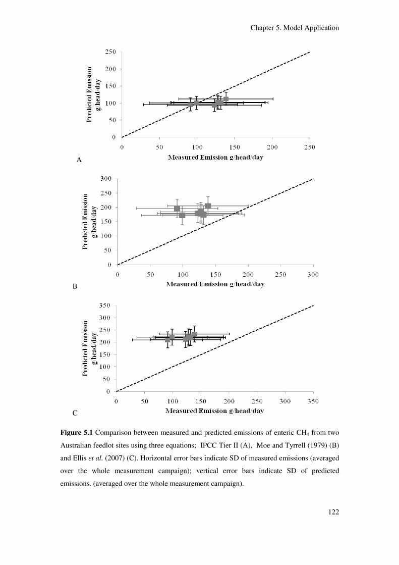
Chapter 5. Model Application
122
A
B
C
Figure 5.1 Comparison between measured and predicted emissions of enteric CH4 from two
Australian feedlot sites using three equations; IPCC Tier II (A), Moe and Tyrrell (1979) (B)
and Ellis et al. (2007) (C). Horizontal error bars indicate SD of measured emissions (averaged
over the whole measurement campaign); vertical error bars indicate SD of predicted
emissions. (averaged over the whole measurement campaign).
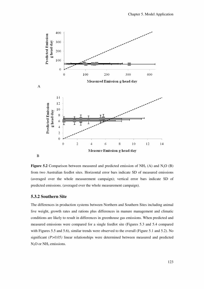
Chapter 5. Model Application
123
A
B
Figure 5.2 Comparison between measured and predicted emission of NH3 (A) and N2O (B)
from two Australian feedlot sites. Horizontal error bars indicate SD of measured emissions
(averaged over the whole measurement campaign); vertical error bars indicate SD of
predicted emissions. (averaged over the whole measurement campaign).
5.3.2 Southern Site
The differences in production systems between Northern and Southern Sites including animal
live weight, growth rates and rations plus differences in manure management and climatic
conditions are likely to result in differences in greenhouse gas emissions. When predicted and
measured emissions were compared for a single feedlot site (Figures 5.3 and 5.4 compared
with Figures 5.5 and 5.6), similar trends were observed to the overall (Figure 5.1 and 5.2). No
significant (P>0.05) linear relationships were determined between measured and predicted
N2O or NH3 emissions.

Chapter 5. Model Application
124
Table 5.9 Fitted linear relationships and SE for predicted and measured greenhouse gas
emissions from a Southern Australian feedlot site over four measurement campaigns
Equation y-intercept Slope Significance SE Obs SE Pred
Moe and Tyrell (1979) 213.2 -0.29 P=0.499 11.0 5.5
Tier II 95.3 0.02 P=0.889 4.4 2.2
Ellis et al. (2007) 202.8 0.12 P=0.682 7.6 3.8
N2O 6.2 0.11 P=0.406 0.4 0.2
NH3 62.7 -0.01 P=0.815 4.7 2.3
Concordance (Table 5.10) between all equations and measured emissions were very low,
however a moderate correlation was observed between measured CH4 emissions and
predictions based on Moe and Tyrell (1979). Consistent with the overall analysis Cb was
highest for estimated based on Tier II. Concordance between measured and predicted values
for both N2O and NH3 are lower at the Southern Site compared with overall estimates, as is
correlation between measured and predicted N2O (0.59) compared with (0.76, overall
correlation).
Table 5.10 Concordance and correlations between predicted and measured greenhouse gas
emissions from a Southern Australian feedlot site over four measurement campaigns
Equation Concordance Correlation Cb
Moe and Tyrell (1979) -0.03 -0.50 0.07
Tier II 0.03 0.11 0.26
Ellis et al. (2007) 0.01 0.22 0.02
N2O 0.05 0.59 0.09
NH3 -0.01 -0.19 0.03

Chapter 5. Model Application
125
A
B
C
Figure 5.3 Comparison between measured and predicted emissions of enteric CH4 using
IPCC Tier II (A), (Moe and Tyrrell 1979) (B) and (Ellis et al. 2007) (C) from a southern
Australian feedlot site. Horizontal error bars indicate SD of measured emissions (averaged
over the whole measurement campaign); vertical error bars indicate SD of predicted
emissions. (averaged over the whole measurement campaign). .

Chapter 5. Model Application
126
A
B
Figure 5.4 Comparison between measured and predicted emissions of NH3 (A) and N2O (B)
from a southern Australian feedlot site. Horizontal error bars indicate SD of measured
emissions (averaged over the whole measurement campaign); vertical error bars indicate SD
of predicted emissions. (averaged over the whole measurement campaign).
5.3.3 Northern Site
No significant (P>0.05) linear relationships (Table 5.11) were observed between measured
and predicted emissions of enteric CH4 at the Northern Site (Figure 5.5 and 5.6).. The linear
relationship between measured and predicted emission of N2O approached significance
(P=0.071).

Chapter 5. Model Application
127
Table 5.11 Fitted linear relationships and SE for predicted and measured greenhouse gas
emissions from a Northern Australian feedlot site over four measurement campaigns.
Equation y-intercept Slope Significance SE Obs SE Pred
Moe and Tyrell (1979) -98.0 2.16 P=0.460 14.8 8.5
Tier II -26.2 0.99 P=0.293 3.8 2.2
Ellis et al. (2007) 16.9 1.56 P=0.154 3.0 1.7
N2O 5.8 0.21 P=0.131 0.13 0.1
NH3 82.3 2.29 P=0.071 0.66 0.4
The highest concordance for measured and predicted (Table 5.12) enteric CH4 emissions was
observed for the Tier II equation (0.07) consistent with the lowest residuals for this equation.
The strongest correlations between measured and predicted CH4 emissions were observed for
the Ellis et al. (2007) (0.97) and Tier II equations (0.90), although Moe and Tyrrell (1979)
also showed a moderate correlation (0.75). Correlation between measured and predicted N2O
emissions was higher at the Northern Site (Table 5.12) than the Southern Site as was the
correlation between measured and predicted emissions of NH3.
Table 5.12 Concordance and correlations between measured and predicted greenhouse gas
emissions from a Northern Australian feedlot site over four measurement campaigns.
Equation Concordance Correlation Cb
Moe and Tyrell (1979) 0.04 0.75 0.05
Tier II 0.07 0.90 0.08
Ellis et al. (2007) 0.01 0.97 0.01
N2O 0.14 0.98 0.14
NH3 -0.05 -0.99 0.05

Chapter 5. Model Application
128
A
B
C
Figure 5.5 Comparison between measured and predicted emissions of enteric CH4 using
IPCC Tier II (A), Moe and Tyrrell (1979) (B) and Ellis et al. (2007) (C) from a northern
Australian feedlot site. Horizontal error bars indicate SD of measured emissions (averaged
over the whole measurement campaign); vertical error bars indicate SD of predicted
emissions. (averaged over the whole measurement campaign). .

Chapter 5. Model Application
129
A
B
Figure 5.6 Comparison between measured and predicted emissions of NH3 (A) and N2O (B)
from a northern Australian feedlot site. Horizontal error bars indicate SD of measured
emissions (averaged over the whole measurement campaign); vertical error bars indicate SD
of predicted emissions. (averaged over the whole measurement campaign). .
5.3.4 Seasonal Differences
During both summer and winter, no significant (P>0.05) linear relationships could be
determined between measured and predicted CH4 emissions for the range of data evaluated.
During winter, significant linear relationships (P <0.05) were determined between measured
and predicted values of NH3 and N2O. During summer a significant relationship (P <0.05)
was only observed for NH3. During winter, the strongest concordance was observed between
measured values and predictions based on Tier II (0.16), although this was not strong.
Concordance between measure and predicted values of NH3 and N2O were very low, despite
strong correlations (N2O 0.96 and NH3 -0.71). A similar effect was observed during summer,
with low concordance, but strong correlations (N2O 0.67 and NH3 0.86). A strong correlation

Chapter 5. Model Application
130
was observed for measured and predicted enteric emissions based on the Tier II equation
(0.99) and a strong negative correlation for Moe and Tyrell (1979) equation (-0.94).
5.3.6 Combined Data
In Chapter 4 the National Inventory Methodology (AGO 2006) for predicting greenhouse gas
emissions (CH4, N2O and NH3) was evaluated using the results of published studies. This
evaluation indicated that for prediction of CH4 emission utilising an equation based on the
CHO fractions in the ration provided the most accurate estimates, although an over estimation
was observed for CHO based equations and an under estimation for the Tier II (3% GEI)
equation. This was consistent with the results of the application of the model to Australian
measurements as described in this Chapter . .
Insufficient published data was available to validate the accuracy of estimates of N2O
emission. However, combining published estimates emissions of NH3 with the measured data
demonstrated that estimates were more accurate (predictions closer to measured values) at
lower emissions levels; however the results of the validation exercise suggested that a single
emission factor to estimate either N2O or NH3 does not allow the impact of environmental
conditions on emissions to be accounted for. This leads to inaccuracies in estimates, despite
the methodology producing reasonable estimates of N excretion.
Examination of the combined dataset (Figure 5.7 and 5.8) demonstrates the similarity of
measured CH4 emissions (Figure 5.7) to those reported in the literature, and consistency of
predicted emissions based on the three equations utilised in this evaluation. Variability
(standard deviations as shown in error bars) was also similar between the measured emissions
reported in this Chapter (5), Chen et al. (2009) and the published studies. The combination of
the published emissions data (and corresponding models) and the measured emissions/
predictions results in changes in the significance of linear relationships; using the combined
data (Table 5.13) a significant (P<0.01) linear relationship was determined between measured
and predicted emissions based on the equation of Moe and Tyrrell (1979). Despite no
significant (P>0.05) linear relationship being observed for the Tier II equation standard errors
of observation and prediction were comparable to those for Moe and Tyrrell (1979). Using the
combined data, estimates of enteric CH4 based on Ellis et al. (2007) were less accurate than
those for the Australian data, reflecting reduced accuracy in the published predictions.
A significant linear relationship (Table 5.13) was observed between the combined measured
and predicted data for N2O. In contrast to the published data there was no significant
relationship between measured and predicted emissions of NH3 using the combined data set.

Chapter 5. Model Application
131
Table 5.13 Fitted linear relationships and SE for measured and predicted emissions of CH4,
N2O and NH3 based on published values and measurements from two Australian feedlots over
seven measurement campaigns. Predicted emission of CH4 is based on three equations.
Equation y-intercept Slope Significance SE Obs SE Pred
Moe Tyrell (1979) 127.8 0.48 P=0.003 21.6 4.6
Tier II 65.6 0.16 P=0.287 21.8 4.7
Ellis et al. (2007) 154.7 0.23 P=0.402 41.0 8.7
N2O 36.2 0.15 P<0.001 10.1 2.4
NH3 6.1 0.13 P=0.170 0.502 0.2
The highest concordance (Table 5.14) between measured and predicted emissions of enteric
CH4 was observed for predictions based on Moe and Tyrrell (1979), consistent with the
results of the published studies (Chapter 4) a similar correlation (0.60 compared with 0.62)
was also observed. Predictions of enteric CH4 using both Tier II and Ellis et al. (2007)
showed low concordance and correlations (0.10 and 0.23 for Tier II and 0.09 and 0.18 for
Ellis et al. (2007) when the combined data set was examined. Concordance between measured
and predicted emissions of NH3 (0.17) increased compared with the Australian feedlot data (-
0.01), but decreased compared with published data (0.29). Utilising the combined data set
decreased concordance between measured and predicted emission of N2O (0.06 compared
with 0.07); however correlation was reduced (0.50 to 0.76).
Table 5.14 Concordance and correlations between measured and predicted emissions of CH4,
N2O and NH3 based on published data (as used in the evaluation reported in Chapter 4) and
measurements from two Australian feedlots over seven measurement campaigns.
Equation Concordance Correlation Cb
Moe and Tyrell (1979) 0.20 0.60 0.33
Tier II 0.10 0.24 0.41
Ellis et al. (2007) 0.09 0.19 0.47
N2O 0.06 0.50 0.12
NH3 0.17 0.78 0.22

Chapter 5. Model Application
132
A
B
C
Figure 5.7 Comparison between measured and predicted enteric methane emissions based on
a database of published studies (literature), and measurements from two Australian feedlot
sites (Aus). Predictions were based on three equations IPCC Tier II (A), Moe and Tyrrell
(1979) (B) and Ellis et al. (2007) (C).

Chapter 5. Model Application
133
A
B
Figure 5.8 Comparison between measured and predicted emissions of nitrogenous gases; NH3
(A) and N2O (B) from a database of published studies (Literature) and measurements from
two Australian feedlot sites (Aus).
5.4 Discussion
This Chapter aimed to apply the predictive equations examined in the previous Chapter (4) to
data collected from two Australian feedlots over seven measurement campaigns, and
compared predictions to measured emissions during these periods. Sources of variation in
measured emissions between sites and seasons were also examined.
5.4.1 Measured Emissions
Measured CH4 emissions are assumed to represent primarily enteric CH4 as manure CH4 was
estimated to contribute less than 2 g/head/day (Hao et al. 2001a). Measured emission from the
Southern Site averaged 110 g/head/day, whilst emissions from the Northern Site averaged 132
g/head/day (excluding summer 2008, 64 g/head/day).

Chapter 5. Model Application
134
Using calorimetric methods Beauchemin and McGinn (2005) measured emissions from high
grain rations of 62 g/day (corn based) and 80 g/day (barley based) and 170 g/day (corn based)
and 130 g/day (barley based) high forage diets. Similarly Boadi et al. (2004b) measured
emissions of 90 g/head/day and 128 g/head/day (for high and low grain rations) using
calorimetric methods. Beauchemin and McGinn (2006) reports emissions of 114 g/head to
169 g/head and Hegarty et al. (2007) report emissions from Australian feedlot cattle
(measured using SF6) of 142 g/head/day (low intake, 8.4 kg DM/head) and 190 g/head/day
(high intake 14.1 kgDM/head/day). McGinn et al. (2007) used micrometeorological methods
to measure CH4 emissions from feedlots in both Australia (also reported by Loh et al. 2008)
and Canada reporting 166 g/head/day for the Australian feedlot, and 214 g/head/day for the
Canadian feedlot.
Emissions measured during the seven measurement campaigns are consistent with enteric
emissions reported for beef feedlot cattle of similar weights and intake levels. The high grain
diets evaluated by Beauchemin and McGinn (2005) with reported emissions of 62 and 80
g/head/day demonstrated very low intakes (5.3 to 6.9 kg DM/day) compared with those
during the measurement campaigns reported here (9-10 kg DM/day at the Southern Site, and
10–11 kg DM/day at the Northern Site). Reduced intakes are consistently cited as an effect of
using calorimetric methods, with alterations to animal feeding behaviour and energy
requirements due to reduced activity. Beauchemin and McGinn (2005) observed reductions in
intake of 31% on a high forage diet, and 22% on a high grain diet when animals were moved
to calorimetric chambers for measurements. Measured emissions reported in this study are
consistent with those reported by Hegarty et al. (2007) and Boadi et al. (2004b) where intakes
and live weights are similar to those reported by the feedlot operators during the measurement
campaigns.
Emissions of CH4 vary both between site and season; although there does not appear to be any
distinct seasonal trends in emissions. However, emissions during 2007 at the Southern Site
were higher (123 and 128 g/head/day) than those in 2006 (989 g/head/day) and 2008 (91
g/head/day). The major difference between these measurement periods where reported
intakes, live weights and target live weight gains were similar was the grain types and average
grain proportion in the rations. During 2007, average grain concentration was 61%, compared
with 70 and 71% during the other measurement periods, whilst barley was the primary grain
source in 2007, compared with wheat for the other campaigns. Whilst Beauchemin and
McGinn (2005) determined a significant difference in emissions between barley and corn
diets due to differences in the fermentative properties of the grain. The difference between
wheat and barley; slightly higher cellulose (46.6 cf. 21.4 g/kg DM) and lignin (17.0 cf. 11.2

Chapter 5. Model Application
135
g/kg DM) in barley and higher starch (674.1 cf. 561.7 g/kg DM) in wheat (Givens and Moss
1990) are likely to be less pronounced than differences between barley and maize (corn).
Maize (corn) contains more rumen protected starch, reducing starch digestibility in the rumen,
depending on processing method (Archibeque et al. 2006). Starch digestion in the rumen is
affected by both starch concentration and physical form of the starch containing grain (Oba
and Allen 2003) although starch concentration is higher in grain such as sorghum and maize
(compared to wheat or barley) it is less available due to enclosure by a hard endosperm (Oba
and Allen 2003; Remond et al. 2004). Less available starch passes to the intestine, where it is
degraded (with variable efficiency); without contributing to rumen fermentation. Although
this does not explain differences in emissions observed between measurement campaigns at
the Southern Site, it may contribute to differences in emissions between northern and southern
feedlot systems, where different base grains are utilised.
There is little difference in the average calculated concentrations of soluble residue, cellulose,
hemicellulose and lignin between the average ration fed during each measurement campaign
at the Southern Site. However, the lower grain concentration (9-10% difference) in the
rations during this period is likely to result in differences in fermentation patterns, primarily
associated with higher available starch, and an increase in hydrogen and CH4 production
which may not be reflected in a simple examination of dietary properties. Measured emissions
at the Northern Site were more similar between measurement campaigns, which appear to
reflect greater consistency of dietary grain concentration (79-81%). A strong negative
correlation (-0.96) was observed between grain concentration and measured emission
(g/head/day) for the Southern Site, which is commonly observed in both beef and dairy cattle
(Beauchemin and McGinn 2005).
Todd et al. (2008) measured NH3 emission rates from a commercial feedlot in the Southern
high plains of Canada and determined mean summer emissions of almost twice those in
winter. In general, emissions were higher during summer (117 and 130 g/head/day) than
winter (51 and 84 g/head/day). Similarly, McGinn et al. (2007) used micrometeorological
measurements and a dispersion model to measure NH3 emissions from a Canadian feedlot
during Summer, and determined emissions averaging 140 g/head/day. Emissions measured
during the 8 measurement campaigns were similar to these results (excluding the Northern
Site summer 2008 and the Southern Site winter 2007), although there did not appear to be any
distinct seasonal trends for these sites. Excluding emissions measured at the Northern Site in
summer 2008 (as discussed above) NH3 emissions from the Northern Site averaged 123
g/head/day compared with 178 g/head/day from the Southern Site.

Chapter 5. Model Application
136
Ammonia emissions can be expressed as a percentage of animal N intake, Todd et al. (2008)
report NH3 emissions annually of 53% of N intake (32 to 72%). Whilst other studies report
NH3 losses as a percentage of total N intake to be between 29 and 63% (Cole et al. 2006;
Flesch et al. 2007; Todd et al. 2008; Todd et al. 2005). Within site, N intakes were similar
(13 to 13.5% CP for the Southern Site, 13.4 to 13.7% Northern Site), despite larger difference
in NH3 emissions between sites and seasons (within sites). This contrasts with the
observations of Todd et al. (2008); where despite similar N intake NH3 loss (g/head/day) was
30-40% higher during summer than in winter. This indicates that differences in manure
management and climatic conditions are primarily responsible for the differences in NH3
observed (although this may not be seasonally dependant). NH3 emissions were more strongly
correlated with humidity (min 0.64, max 0.54) and wind (-0.67) than min or max temperature
(min -0.44, max -0.21) and rainfall (-0.24; Todd et al. (2008).
Measured N2O emissions from both sites were variable, averaging 2.6 g/head/day at the
Southern Site (0.1 to 5.3 g/head/day) and 3.6 g/head/day (1.6 to 5.7 g/head/day) at the
Northern Site (excluding summer 2008, 4.8 g/head/day). Boadi et al. (2004b) reports N2O
emissions equivalent to 0.16 and 0.15 g/head/day. However, these measurements were based
on small chamber measurements (in situ). Chambers were 20 cm diameter, and 6 used in each
pen area. There is considerable spatial variation within a single pen, therefore the chamber
measurements may not reflect potential emissions from the whole surface. Further,
environmental conditions (reported as cold temperatures, averaging 0.4, -8.0 and -6.4 °C for
the three measurement periods (Boadi et al. 2004b)) are considerably lower than those
observed in the measurement campaigns reported here, which is likely to limited microbial
activity in the observations of Boadi et al. (2004b).
There is a significant lack of published information regarding the loss of N2O from feedlot
surfaces, although an increasing number of studies (Chadwick 2005; Hao et al. 2001a) have
examined losses from manure composting, spreading and effluent systems (mostly for housed
dairy cattle; Jungbluth et al. 2001; Kulling et al. 2003). In general, measurements of
nitrogenous gas loss from feedlot systems focus on the volatilisation of NH3, which although
considered a direct greenhouse gas, is a secondary source of N2O, and an environmental
polluter. The association between NH3 and other malodorous volatile compounds produced in
feedlot systems is likely to result in calls for a reduction in NH3 (McGinn et al. 2003). Further
investigation is required into the deposition of NH3 (and potential N2O emissions) as well as
the impact of a reduction in NH3 volatilisation on direct N2O emissions. In this study there
was a moderate negative correlation (R2 -0.68) between emissions of NH3 and N2O (over 7
measurement campaigns). Conditions which favour volatilisation result in decreased N

Chapter 5. Model Application
137
concentrations in the manure pad/ soil substrate, reducing available N. This moderate
correlation indicates that practices which decrease NH3 volatilisation may in fact increase
direct N2O loss (although feedlot conditions generally do not favour N2O production), which
has more significant consequences as a greenhouse gas.
5.4.2 Emissions Prediction
In Chapter 4, which evaluated the prediction equations for enteric CH4, N transactions and
emission of nitrogenous gases, it was concluded that using an equation based on the
carbohydrate concentration/ composition (e.g. Moe and Tyrell 1979 and Ellis et al. 2007)
improved emissions estimates (based on concordance, which is a measure of both the
correlation between the values and the slope and origin of the line). The Tier II equation
demonstrated the lowest SE of prediction and observation, suggesting low residuals and
improved accuracy of estimates, however concordance was reduced compared to CHO based
equations. It was concluded that utilising an equation based on the CHO composition of the
ration would improve estimates compared with the energy based models.
For the measurement campaigns and periods of data collection at Australian feedlots utilised
here the Tier II equation appears to provide the most reasonable estimates. The Tier II
equation demonstrates the highest concordance observed (utilising Australian measurements)
between measured and predicted emissions. As detailed in the general methodology the Tier
II equation estimates enteric CH4 emission based on intake of Gross Energy, and a CH4
conversion factor, which is loosely based on ration type. A value of 3 ± 1% of gross energy is
prescribed for feedlot cattle consuming a high (greater than 90%) grain diet. The primary
difference between the range of studies utilised in the evaluation, and those fed in the
measurement campaigns outlined here is the content of grain in the rations. Using the Tier II
predictions (Figure 5.3) at the Southern Site as an example (and based on the trends discussed
above) the need for an emission factor which considers grain concentration at an individual
site is demonstrated clearly. For the lower measured emissions (and higher grain
concentrations) predictions demonstrate residuals of less than 5 g/head/day. Higher measured
emissions (and high grain concentration) show residuals closer to 30 g/head/day. The Tier II
equation is suggested by the IPCC for diets with grain concentrations above 90%, however
the range of grain concentrations for which this is effective has not been established.
Although studies selected for validation were those feeding “feedlot type” rations, the overall
grain content ranged from 30 to 90% (65% average), which is likely to result in
underestimation in predicted emissions at the lower end of grain concentration. Average grain
percentages reported over the 8 measurement campaigns at the Northern and Southern

Chapter 5. Model Application
138
feedlots ranged from 61 to 81%, which is consistent with improved predictive ability for
higher grain rations.
The evaluation of the model for nitrogen transactions in Chapter 4 suggested that whilst faecal
excretion (and retained N) was poorly estimated overall N excretion could be predicted quite
accurately (concordance 0.94). Due to the measurement methods utilised for this study,
detailed examination of N excretion was not able to be undertaken, however based on the
evaluation in Chapter 4, it is assumed that excretion is being estimated accurately. The aim of
this section was therefore to examine the accuracy of the emission factors applied to excreted
N in order to predict NH3 and N2O emission. The implication of using a single emission factor
to estimate volatilisation of NH3, which is affected not only by excreted N, but by
environmental conditions, is demonstrated clearly by these results. At low levels of measured
NH3 accuracy of prediction is reasonable, however as measured NH3 increases the ability of
the model to predict emission decreased substantially. A significant linear relationship could
not be determined (P>0.05), and both concordance (0.005) and correlation (0.15) were low.
This effect can be considered to be primarily due to the use of the single emission factor (0.3)
which does not reflect the wide range of environmental conditions influencing NH3
volatilisation (temperature, moisture, pH). Measured NH3 emissions range from 94 ± 2.8
g/head/day to 324 ± 34.7 g/head/day (mean and SE), with no distinct seasonal or site trends.
Percentage loss of NH3 has been reported to vary between 29 and 60% of N intake, and up to
70% of N excreted (McGinn et al. 2007); this alone suggests the difficulty in setting a single
emissions factor.
As reported by McGinn et al. (2007) a significant factor contributing to the under estimation
of NH3 emissions may be related to accumulated manure in the pens. Although the majority
of NH3 is quickly volatilised, the accumulated manure may still be a source of volatile NH3.
These emissions are not accounted for by the empirical equation utilised in the methodology.
There is also a difference in manure management strategies between sites, which is likely to
contribute to differences in measured emissions, and in accuracy of prediction. The chemical
composition of manure is also affected by animal size, age and condition, water consumption,
feedlot surface, animal density, amount of type of bedding and handling of the manure/
surface (Miller et al. 2003). Volatilisation of NH3 is influenced by not only N excreted (and
available in the substrate) but by ambient and substrate temperature, pH and moisture content,
leading to considerable variation not only with a day, but between site and season. The use of
a single emission factor, and similarity in ration crude protein, weight gain and feed offered
results in very low variability in predicted volatile NH3, which is not reflective of the
biological variability.
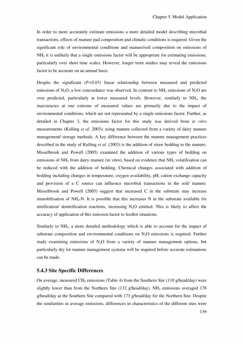
Chapter 5. Model Application
139
In order to more accurately estimate emissions a more detailed model describing microbial
transactions, effects of manure pad composition and climatic conditions is required. Given the
significant role of environmental conditions and manure/soil composition on emissions of
NH3 it is unlikely that a single emissions factor will be appropriate for estimating emissions,
particularly over short time scales. However, longer term studies may reveal the emissions
factor to be accurate on an annual basis.
Despite the significant (P<0.05) linear relationship between measured and predicted
emissions of N2O, a low concordance was observed. In contrast to NH3 emissions of N2O are
over predicted, particularly at lower measured levels. However, similarly to NH3, the
inaccuracies at one extreme of measured values are primarily due to the impact of
environmental conditions, which are not represented by a single emissions factor. Further, as
detailed in Chapter 3, the emissions factor for this study was derived from in vitro
measurements (Kulling et al. 2003); using manure collected from a variety of dairy manure
management/ storage methods. A key difference between the manure management practices
described in the study of Kulling et al. (2003) is the addition of straw bedding to the manure.
Misselbrook and Powell (2005) examined the addition of various types of bedding on
emissions of NH3 from dairy manure (in vitro), based on evidence that NH3 volatilisation can
be reduced with the addition of bedding. Chemical changes associated with addition of
bedding including changes in temperature, oxygen availability, pH, cation exchange capacity
and provision of a C source can influence microbial transactions in the soil/ manure.
Misselbrook and Powell (2005) suggest that increased C in the substrate may increase
immobilisation of NH4-N. It is possible that this increases N in the substrate available for
nitrification/ denitrification reactions, increasing N2O emitted. This is likely to affect the
accuracy of application of this emission factor to feedlot situations.
Similarly to NH3, a more detailed methodology which is able to account for the impact of
substrate composition and environmental conditions on N2O emissions is required. Further
study examining emissions of N2O from a variety of manure management options, but
particularly dry lot manure management systems will be required before accurate estimations
can be made.
5.4.3 Site Specific Differences
On average, measured CH4 emissions (Table 4) from the Southern Site (110 g/head/day) were
slightly lower than from the Northern Site (132 g/head/day). NH3 emissions averaged 178
g/head/day at the Southern Site compared with 173 g/head/day for the Northern Site. Despite
the similarities in average emissions, differences in characteristics of the different sites were

Chapter 5. Model Application
140
hypothesised to result in differences in the accuracy of the various equations utilised in the
prediction of enteric CH4 emissions. The major differences in animal characteristics between
the sites are the average live weight (440 to 520 kg at the Southern Site compared with 530 to
750 kg at the Northern Site, Table 5.2), offered feed amount (9.8 kg DM/head/day Southern
Site, 10.7 kg DM/head/day Northern Site), the grain content of the rations Table 5.5) and the
types of grains used (predominately wheat at the Southern Site and sorghum at the Northern
Site). Climatic conditions vary between sites; temperatures (both minimum and maximum)
were higher and less variable at the Northern Site. Average wind speed and summer gust
speed was faster at the Northern Site, potentially increasing diffusion gradients by removing
emitted gases from the surface.
The slightly higher CH4 emissions measured at the Northern Site could be attributed to the
higher live weights and intakes observed. Average CH4 emissions at the Northern Site
equated to 12.4 g CH4/kg DM compared with 11.2 g CH4/kg DM intake at the Southern Site,
the additional 0.8 kg DMI at the Northern Site could be expected to increase average CH4
output by 9.3g/day to 119 g/day (based on average production CH4 g/kg DM at the Southern
Site). This indicates that the higher CH4 emissions observed are not simply an artefact of
higher intakes.
The effect of a different grain type cannot be ignored. The previous discussion focused on the
difference between emissions associated with wheat or barley based rations at the Southern
Site, however the small difference in fermentative characteristics (considered as starch,
cellulose and hemicellulose as these are key model components) between wheat and barley
was considered unlikely to be the primary cause of the differences in measured emissions
between years. Grain concentration of rations showed a strong negative correlation with
measured emission at the Southern Site. However, a more significant difference exists in
grain types between sites. Grains at the Northern Site are predominantly sorghum, whilst
wheat and barley are more common at the Southern Site. Sorghum contains considerably
higher starch (730 g/kg DM) than barley (560 g/kg DM), more comparable to maize grain
(699 g/kg DM), although lignin is considerably lower in maize (6.3 g/kg DM) than in
sorghum (23.8 g/kg DM; Givens and Moss 1990).
Differences in metabolism between tropical (Bos Indicus) and temperate (Bos Taurus) type
cattle may contribute to differences in emissions between sites. Typical of Northern
Australian feedlots, the Northern Site contained tropical breeds (e.g. Brahman) during all
measurement campaigns, while the Southern Site contained predominantly temperate/ British
breeds (e.g. Angus and Hereford). Kurihara et al. (1999) reports that relationships between

Chapter 5. Model Application
141
CH4 production, energy utilisation and live weight of Bos Indicus (tropical) cattle when fed
tropical forages (e.g. Ruzi grass and Rhoades grass) differ from those of Bos Taurus cattle fed
temperate forages, however they do not report comparative CH4 production for tropical cattle
fed temperate forages. Hunter (2007) in a letter regarding the results of Kurihara et al. (1999)
this indicate that CH4 production from tropical cattle fed high grain diets (per unit of gross
energy intake) is higher than for Bos Taurus cattle. The high number of tropical cattle in the
Northern Australian production system is likely to be a contributing factor to the higher
emissions observed at this site, and particularly the higher emissions/kg DMI.
The Tier II equation could be expected to more accurately predict emissions from the
Northern Site; due to the higher grain content (71-81%), compared to the Southern Site (61 to
71%). The Tier II equation demonstrates the highest concordance (Table 5.12) of the CH4
prediction equations evaluated for both sites. However, closer examination of the predictions
for individual measurement campaigns shows underestimation of emissions. Similarly to the
overall analysis, no significant (P>0.05) linear relationships were determined between
measured and predicted emissions at either site. Concordance was significantly reduced for
all CH4 prediction equations at both sites. From the Southern Site, the lowest standard errors
(of observation and prediction) were observed for Tier II (4.35 and 2.17); however Ellis et al.
(2007) showed the lowest standard errors (observation and prediction) and highest correlation
for the Northern Site. These results suggest that the difference in composition of rations (the
major difference between sites in terms of CH4 emission), particularly the source of grain,
influences the accuracy of emissions estimates. Specifically, the distinct variation in
emissions related to grain type reported by Beauchemin and McGinn (2005) and observed to
some extent in this study (sorghum vs. barley), as well as forage concentration, suggests that
utilising an equation based on ration nutrient fractions, even when these are estimated, will
probably allow more accurate estimates of CH4 output based on the individual site
characteristics.
Although Tier II shows the highest concordance at the Northern Site, the reduced accuracy, as
indicated by higher standard errors of observation and prediction compared to the Southern
Site, may be influenced by the factors discussed above in the context of between site
differences. Such as alterations in fermentative characteristics of grain types (sorghum
compared with wheat or barley) and in the metabolism of tropical compared with temperate
cattle breeds.
Ammonia emissions from the Northern Site averaged 123 g/head/day, compared with 178
g/head/day from the Southern Site. Nitrous oxide emissions averaged 2.6 g/head/day from the

Chapter 5. Model Application
142
Southern Site and 3.6 g/head/day from the Northern Site. The primary factors influencing
emissions of N2O and volatilisation of NH3 are N content (N excretion), moisture content,
temperature, pH, soil compaction, oxygen availability and microbial activity. These factors
are all likely to vary both between and within sites, and contribute to the differences in
emissions observed.
Nitrogen intakes were similar between sites, 212 to 233 g/head/day (averaging 223
g/head/day) at the Southern Site and 222 to 250 g/head/day (averaging 233 g/head/day) at the
Northern Site. The slightly higher N intake at the Northern Site could be expected to result in
higher NH3 emissions, however this was not observed. Over feeding N relative to
requirements results in increased excretion of N, primarily in the urine, this is readily volatile
as NH3. The difference in fed N g/kg live weight (0.42 Northern Site, 0.47 Southern Site)
indicates that feeding level of N is slightly higher at the Southern Site; however it would be
unlikely to contribute to the magnitude of difference observed in emissions. Consistently,
estimated N excretion (calculated based on the modelling approach described) was similar
between sites (204 g/head/day south, 208 g/head/day north). Ammonia emissions equate to
87% (south) and 59% (north) of excreted N, or 80% and 53% of N intake. The Southern Site
values are considerably higher than the normal range reported. However, NH3 emissions
measured using micrometeorological methods reflect not only freshly deposited manure but
built up manure in pens, which may contribute significantly to total emissions. Manure pad
management differed between the sites, manure was observed to be more built up in pens at
the Southern Site, which were generally scraped clean after individual “lots” of cattle leave
the feedlot. In contrast, pens were cleaned more frequently at the Northern Site, with manure
mounded in the centre of pens. The less frequent cleaning results in a wetter, deeper and more
variable surface. As discussed by McGinn et al. (2009) this build up of manure is likely to
contribute to higher measured NH3 emissions. Less frequent cleaning and manure build up
also changes the composition of the manure pad below at the surface. Todd et al. (2005)
report that NH3 volatilisation in the feedlot comes from a pool of rapidly hydrolysed urea,
replenished regularly by urination, and from NH4 mineralised from organic forms. Built up
manure is likely to contain organic N, which can be mineralised (a slower process) to provide
a more constant source of NH3 (Todd et al. 2008).
The lower N2O emissions observed at the Southern Site (and higher at the Northern Site)
reflect the greater loss of N (in the form of NH3) at the Southern Site, where conditions appear
to favour volatilisation over nitrification/ denitrification. Stewart (1970) determined that
under laboratory conditions the amount of NH3 volatilised and nitrate (NO3) accumulated
depended on the moisture content of the soil/ substrate; when urine was added to dry soil (at 4

Chapter 5. Model Application
143
day intervals) more than 90% of N was lost as NH3. When soil was initially wet about 65% of
N was converted to nitrate. However, Miller and Berry (2005) determined that at very low
moisture contents nitrogenous compounds were less likely to volatilize or convert to more
volatile forms, and that increased moisture enhanced the volatilisation of NH3.
Miller and Berry (2005) also determined that manure content (in the soil pan incubations)
altered the effect of moisture on greenhouse gas emissions (CH4 and N2O), suggesting that
with increased manure content (relative to the soil in the incubation) water availability for
microbial activity decreased. At low manure contents under fermentative (high moisture)
conditions, N2O was the dominant greenhouse gas emission, whilst at high (75%) manure
concentration N2O emissions were absent. Consistently, Adams et al.(2004) determined that
more frequent pen cleaning reduced N losses from open yard feedlots (and compost). This
supports the observation that higher NH3 loss at the Southern Site, associated with a greater
build up of manure, further these observations go some way to explaining the differences in
N2O observed between sites. The more frequently cleaned, lower manure substrate at the
Northern Site (which was observed in most campaigns to be drier) showed higher average
emissions whilst the generally higher manure surface at the Southern Site showed lower
average emissions. Additionally, Saggar et al. (2004b) reports increased N2O emissions at
higher temperatures, consistent with the higher average temperatures at the Northern Site.
Differences in animal characteristics, manure management practices and ration composition
are likely to result in differences in accuracy of emission prediction between the sites (Boadi
et al. 2004b). Although NH3 was consistently under estimated, and N2O consistently over
estimated, the range in measured values (at a quite constant predicted value) highlights the
issues with using a single emission factor. As discussed, predicted N excretion (based on
animal and dietary parameters) is multiplied by an emissions factor. The differences in
accuracy (as indicated by concordance) between sites, for both NH3 and N2O concordance
was slightly higher for the Northern Site, perhaps indicates that if a more complex model is
not applied, then a site specific parameter should be used. This approach is utilised for
prediction of manure CH4 in the National Inventory Methodology (AGO 2006), with different
emissions factors for temperate and tropical regions. However, seasonal conditions could be
expected to have a greater impact than site characteristics.
5.4.4 Season Specific Differences
Environmental and climatic conditions have a significant impact on emissions of N2O and
volatilisation of NH3 (Saggar et al. 2004b), which could therefore be expected to contribute to
both site and seasonal differences in emissions, and in the accuracy of a single emissions

Chapter 5. Model Application
144
factor. Miller et al. (2003) determined chemical properties of feedlot manure to be
significantly different between seasons, including total C and P, NO3-N, NH4-N. Bacterial
content of the manure was also seasonally affected, including numbers of E.coli and total
coliforms. Saggar et al. (2004b) measured soil moisture, temperature, N availability and
soluble C in dairy pastures during four seasons and determined that N input and water filled
pore space were the factors which most affected N2O emissions. They also determined large
variability throughout the year in both grazed and un-grazed pastures. The differing
composition between seasons is likely to contribute to differences in potential emissions,
moderated by the effects of temperature (Miller et al. 2003).
As discussed above, there does not appear to be a distinct seasonal difference in measured
emissions of NH3. Average NH3 emissions in summer were 129 g/head/day, while average
winter emissions were 173 g/head/day. N2O emissions averaged 2.9 g/head/day in summer,
and 3.2 g/head/day in winter, with considerably greater variability observed between winters
(at both sites) for both gases. Higher emissions of NH3 would be expected when conditions
favour a wetter surface, which promotes NH3 volatilisation (Denmead et al. 2008). However,
a substrate which promotes NH3 volatilisation could be expected to result in decreased N2O
emission.
There was no substantial difference in the crude protein concentration of the rations between
seasons, therefore differences in emissions between seasons is associated primarily with
environmental conditions. Todd et al. (2008) attribute the seasonal differences observed in
their study to increase in dietary N. Increasing CP above requirements increases excretion of
urinary N, of which a large proportion is volatile NH3. In the study of Todd et al. (2008) CP
increased from 13.5 to 15% increasing N intake up 24 g/head/day, and increasing volatile N
loss. However, there was little discussion regarding the impact of environmental or manure
management conditions on these emissions. Crude protein concentrations of the rations (from
the Australian feedlots reported) ranged from 13.0 to 13.7%, with no correlation with season
(R2 < 0.05). This suggests the differences in emissions between sites and seasons are related
more closely to environmental conditions than differences in ration N (crude protein)
concentration. However, it should be noted that live weights and growth rates are lower at the
Southern Site. Despite lower average DMI, cattle at the Southern Site are offered on average
0.98 kg CP/kg gain, compared with 0.85 kg CP/kg gain at the Northern Site. Potentially
contributing to higher NH3 emissions at this site (reduced efficiency of N use).
Significant linear relationships (P<0.05) were determined between measured and predicted
emissions of NH3 for both seasons, however standard errors of prediction suggest Summer

Chapter 5. Model Application
145
estimates were more accurate, supported by higher concordance. The discussion above
suggested a drier surface led to more accumulation of N in the substrate (Miller and Berry
2005) and reduced NH3 emissions (Stewart 1970), suggesting that the conditions in Summer
better represent the current emissions factor. As argued for the site differences, the differences
in accuracy between seasons highlight the need for either a more complex model of NH3
emissions. This model needs to account for not only differences in composition associated
with seasonal conditions, but with the contribution of built up manure, and differences in pen
cleaning interval.
Significant (P<0.05) linear relationships were determined for emissions of N2O separated by
summer and winter (SE of both observation and prediction was decreased substantially
compared with the overall data set). However, in contrast to NH3, concordance and
correlation demonstrated more accurate predictions during winter than summer. This suggests
that the 0.02 emission factor is more appropriate for the cooler temperatures and possible
wetter surface (particularly at the Southern Site) observed during winter than the desiccated
surface commonly observed in summer, despite the greater variability in emissions. Saggar et
al. (2004a) determined more variable emissions during winter and spring than the drier
autumn measured. They suggest that a model which accounts for climatic variation in rainfall
and soil texture is better able to predict emissions more accurately than a single emission
factor (Saggar et al. 2004a).
Environmental conditions are likely to have less impact on emissions of CH4 than on the
nitrogenous gases. CH4 emissions averaged 122.9 g/head/day in winter, compared with 115.4
g/head/day in summer. However, as discussed there did not appear to be any seasonal trends
in emissions within site. Alterations in ration composition did not appear to have any distinct
seasonal trends, although there was some difference in types of grain used between years,
particularly at the Southern Site. Alterations in intake behaviour associated with higher day
time temperatures may influence total intake, leading to differing emissions between summer
and winter. Reported intakes average 10.0 kg DM/head/day for the Summer campaigns, and
10.3 kg/head/day for the Winter campaign, resulting in 11.5 g CH4/kg DM during Summer,
and 12.0 g CH4/kg DM during Winter. Blaxter and Wainman (1961) determined that CH4
production did not change in response to environmental temperature (between -5 and 35 °C),
therefore differences between seasons in CH4 emissions appears to be primarily associated
with slight differences in intake. McGinn et al. (2008) reports lower CH4 emissions during
daylight hours from the Northern feedlot utilised in this study, which they attribute to changes
in intake associated with heat stress. They report that shade seeking behaviour, and a
reduction in intake to manage heat load (Mader et al. 2002) may result in reduced intake and

Chapter 5. Model Application
146
therefore lower emissions. This effect is likely to be translated to total daily emissions, which
would not be accounted for in the intake figures reported by the feedlot operators (these are
offered feed amounts kg DM/head/day).
The short term nature of the measurement campaigns contributes to difficulty in making
assumptions regarding seasonal differences in emissions. This is particularly important for the
emissions of nitrous oxide and ammonia . Pulses or peaks of N2O have been observed
following rainfall events in dairy pastures (Saggar et al. 2004a) for long periods after urine/ N
deposition. The short term measurements may (or may not) have captured periods of high
emissions. Longer term monitoring of emissions, N consumption and manure pad
characteristics would increase the ability to asses these emissions and accuracy of emissions
estimates on a longer term basis. However, these results indicate that seasonal differences are
unlikely to have a significant impact on accuracy of enteric CH4 emission prediction, where
they are not associated with substantial changes in ration composition. The consistency of
rations utilised in a feedlot environment should enable the same predictive equation to be used
to estimate emissions on an annual basis, once they are further refined to improve accuracy of
estimates.
5.4.5 Combined Data Set
In contrast to the evaluation based on the two feedlot sites, when the combined data set is
utilised, the equation of Moe and Tyrrell (1979) demonstrates increased accuracy and a
significant linear relationship between measured and predicted emissions. Differences in
accuracy of CH4 prediction equations between the published data and that reported in this
study may be related to the measured animals. Feedlots house animals at varying stages of
growth, size, intakes and rations (Stackhouse et al. 2011) in contrast to the more consistent
animals used in calorimetric measurements. On an individual animal/ pen basis, over a
smaller range of live weights, intakes and rations composition the more specific equation
based on ration composition may prove more accurate. Over an entire feedlot, the simpler
Tier II equation appears to be more “generally” right, although it is less suitable for use with
more specific studies.
5.4.6 Role of DMI
As determined by Bell et al. (2009) daily DMI is highly correlated with live weight and gross
or metabolisable energy intake. Based on the observations discussed previously in this
Chapter, the Tier II equation linking gross energy consumption to CH4 production provides a
reasonable estimate of CH4 emissions over the range of data evaluated. The difference

Chapter 5. Model Application
147
between the approach used here, and that used in the National Inventory Methodology (2006),
is that offered feed was utilised as the predictor of intake, rather than a set value for feedlot
cattle class. In Chapter 4 (section 4.4) this set value was observed to have the lowest
concordance with offered feed, with set values generally considerably higher than offered
feed. However, using a class based estimate of intake improved accuracy of emissions based
on the three best performing equations, compared to offered feed, feed based on live weight
% and feed intake predicted based on growth (Minson and McDonald 1987).
For the data reported utilising a class-based-intake improves the concordance from Moe and
Tyrrell (1979) (from 0.01 to 0.02) and correlation between measured and predicted emissions
(-0.32 compared with 0.07). In contrast, concordance and correlations reduced for Tier II and
Ellis et al. (2007) compared with offered feed based measurements. As Stackhouse et al.
(2011) suggests, the cattle in a feedlot are made up of a range of live weights, intakes, growth
stages and potential emissions. When offered feed is used as a predictor, the Tier II equation
appears to be account for the differences in emissions over the feedlot, providing the most
accurate estimates. When a class-based-intake value is used, it appears to add an additional
layer of uncertainty, decreasing accuracy of estimates. The improvement in estimates based
on (Moe and Tyrrell 1979) with the class-based-intake could potentially be related to the
more specific accounting for ration composition.
5.5 Conclusion
The application of the model to data collected from commercial feedlots highlights the
observations of Mills et al. (2003) that validation of an approach in one situation does not
guarantee accuracy in another. In contrast to the published data evaluated in the previous
Chapter, for an analysis covering both feedlots the Tier II methodology provided the most
accurate estimates. However, this may be attributed in some part to the micrometeorological
measurement method, which encompasses a wider range of animal characteristics, intakes,
rations and potential emissions. The combination of Moe and Tyrrell (1979) and a class-
based-intake prediction is the current methodology for estimating emissions from feedlot
cattle in Australia. This evaluation indicates that while Moe and Tyrrell (1979) shows the best
estimate when a class-based-intake is used; Tier II appears more accurate when a feedlot
average offered feed is applied.
The differences in accuracy of CH4 prediction equations between seasons and sites indicate
that a modified CHO based equation, or a ration specific emission factor (based on grain

Chapter 5. Model Application
148
content) will be more accurate than a single value. However, further research will be required
to determine these for Australian feedlot conditions.
For NH3 and N2O, the application of the model of the data here demonstrates clearly the
primary issue with the approach of the current methodology. The use of a single emissions
factor estimating emissions from excreted N does not allow the effects of manure
composition, management and climatic conditions to be accounted for. The short term nature
of these measurement campaigns means that it is difficult to determine if these single
emissions factors will prove to be accurate on an annual basis (although they are not on a
daily or weekly basis). Similar to CH4, more detailed studies focussing on greenhouse gas
emissions from Australian beef feedlots are required in order to increase reliability of
modelling approaches.

Chapter 6. Behaviour and Emissions
149
Chapter 6. Correlations between Diurnal Patterns of
Greenhouse Gas Emissions and Feeding Behaviour of
Feedlot Cattle
6.1 Introduction
Distinct diurnal emissions patterns have been observed for NH3 and CH4, particularly when
continuous measurements are conducted using micrometeorological techniques. Methane
emissions appear to be cyclical and greatest during periods of rumination (Denmead et al.
2000; Harper et al. 1999). Denmead (1994) observed short term cycles in CH4 production (as
well as a distinct diurnal pattern) of peaks during rumination and troughs during grazing.
Lockyer (1997) reported CH4 emissions which increase during daylight, reaching a peak near
sunset and then declining towards sunrise. NH3 emissions appear to follow the reverse pattern,
being low in the morning and evening and highest during the middle of the day. Flesch et al.
(2007) observed NH3 emissions be low early in the morning, increase into the early afternoon
and then decline until sunset, a similar pattern was recorded by Loh et al. (2008).
Lockyer (1997) compared observed diurnal pattern of CH4 with published records of sheep
grazing behaviour and young cattle and concluded that the pattern of CH4 emissions was
comparable to published grazing behaviour. Methane emissions increased as grazing activity
increased (with the accumulation of feed into the rumen), as rumination or idling increased
following sunset CH4 emission decreased (decrease in rumen contents; Lockyer 1997). A
similar pattern was observed by Murray et al. (1999) who observed an increase in CH4
emissions directly following time of feeding (grass). Murray et al. (1999) also noted a large
flux when animals were fed, which they attributed to displacement of CH4 from the rumen by
the introduction of feed material. Harper et al. (1999) determined that short term variability
in CH4 emissions were primarily related to animal behaviour, however presented only a small
part of the data identifying the correlation between rumination index (rather than total number
ruminating) and CH4 flux. It is well documented that the feeding behaviour of feedlot and
grazing cattle follows a diurnal pattern, and is influenced by temperature and timing of feed
delivery (for housed or feedlot cattle), as well as composition and characteristics of feed, and
social hierarchies (DeVries et al. 2003; Fell and Clarke 1993). Hoffman and Self (1973)
observed the first peak in feeding between 6 and 9 am, followed by a decline between 9 and
12, with a gradual increase to a second peak between 3 and 9 pm. Cattle are generally
observed to most of their eating at sunrise and sunset, particularly during Summer (Gonyou
and Stricklin 1984; Ray and Roubicek 1971). Feeding behaviour is also influenced by season,
primarily due to temperature and photoperiod differences (Gonyou and Stricklin 1984).

Chapter 6. Behaviour and Emissions
150
Hoffman and Self (1973) observed the greatest activity in late afternoon and early evening in
summer, and in later afternoon (3-6pm) in winter. Cattle were also observed to spend more
time under shade in Summer than in winter (Hoffman and Self 1973). Feeding at sunrise and
sunset appears to be relatively independent of the timing of feed delivery (Gonyou and
Stricklin 1984).
However, animal behaviour may not be the only contributing factor to diurnal patterns of
emissions. Measurements undertaken using micrometeorological methods may suffer from
microclimate issues, primarily related to the inversion layer, or increased boundary layer
stability, at night (Flesch et al. 2007; McGinn et al. 2009). This effect appears to be more
pronounced for CH4. Flesch et al. (2007) observed little modulation of emissions related to
temperature and wind speed, citing time of day (and animal activity) as a greater predictor of
NH3 emissions. Knowledge of behavioural patterns and associations with emissions may be
useful in attempting to select a period of the day for short term measurements of emissions
(which are then extrapolated to whole day estimates).
6.1.2 Research Questions
This section aimed to address the following research questions;
1. Is there a significant differences in emissions of CH4 and NH3 between times of day,
which contributes to diurnal flux patterns?
2. How closely correlated are fluxes of greenhouse gas, animal behaviour and
environmental conditions?
6.2 Materials and Methods:
6.2.1 Site Selection
Full details of the sites selected can be found in the General Methodology (Section 3.1).
Behavioural observations were conducted in conjunction with the final winter (2007) and
summer (2008) measurements at both sites.
6.2.2. Animal Characteristics
Observations of animal behaviour took place over two measurement campaigns; winter and
summer at each site (four campaigns in total). A single pen was selected at each site during
each campaign, which was representative of the range (size, days on feed, breed) of cattle
currently on feed at each site.

Chapter 6. Behaviour and Emissions
151
6.2.2.1 Winter 2007
During the first (winter) measurement campaign at the Southern Site the pen contained 247
head of mostly B. Taurus, weight 434-442 kg, minimum 28 DOF. The ration fed contained
69.9% wheat, 12.5% silage, 3.5% grass hay, 5% liquid finisher, 8% cottonseed and 1.1%
vegetable oil; 75% DM, 14.42% CP, 13.15 MJ ME/kg DM. Measured emissions (averaged
over the whole site) were 122.8 g CH4/head/day and 305.1 g NH3/ head/day (Table 5.4). At
the Northern Site the pen contained 161 head of B. Indicus steers with an estimated weight of
477 kg, approximately 30 days on feed. The ration fed comprises 11.5% silage, 0.5% recycled
oil, 1.5% straw, 4.6% liquid supplement, 75.9% sorghum grain and 6% cottonseed; 69.15%
DM, 13.50% CP, 12.76 MJ ME/kg DM. Measured emissions averaged 138.8 g CH4/head/day
and 94 g NH3/head/day (Table 5.4).
6.2.2.2 Summer 2008
During the second measurement campaign the Southern Site contained 223 head of B. Taurus
steers, between 480 and 570 kg and 60 to 75 days on feed. The ration fed contained 27%
wheat, 14% silage, 1.5% grass hay, 4.8 % liquid finisher, 8% cotton seed, 1.1% vegetable oil,
3.1% molasses and 40.5% barley; 73% DM, 13.5% CP, 12.8 MJ ME/ kg DM. Emissions
averaged 91.0 g CH4/head/day, and 102.0 g NH3/head/day (Table 5.4). The Northern Site pen
contained 196 head of B. Taurus steers 642 kg, and 116 days on feed. The ration fed
contained 39% sorghum, 4.5 liquid supplement, 1% straw, 1% cotton hulls, 10% cotton seed,
5% silage, 39% barley and 0.5% recycled oil; 73% DM, 13.83% CP, 12.67 MJE ME/kg DM.
Emissions averaged for the whole site were 63.8 g CH4/head/day and 324.4 g NH3/head/day
(Table 5.4).
6.2.3 Behavioural Observations
Video recording was used for make continuous observations of the pen from sunrise
(approximately 6 am in summer and 7 am in winter) to sunset (6 pm in winter and summer).
Due to the lack of lights observations of feeding behaviour were not possible during the night.
Observations were recorded at 10 minute intervals by stopping the video and counting
number of cattle at the feed bunk (within one m), water trough (within one m), standing and
lying. Walking and “other” were determined by viewing 15 seconds either side of the 10
minute time point and counting the number walking and undertaking activities classified as
‘other’ (grooming, interacting with another animal). Number ruminating was determined
using the same interval, by randomly selecting 20 animals and counting the number

Chapter 6. Behaviour and Emissions
152
ruminating. The proportion determined using this method was then multiplied to give total
number ruminating.
6.2.4 Micrometeorological Measurements
Full details of the micrometeorological and emissions measurements can be found in the
General Methodology (Section 3.2). Briefly, a micrometeorological approach based on
measurements of gas concentrations with open-path gas analysis (tuneable diode lasers and
FTIR) and a backward Lagrangian Stochastic (bLS) dispersion model was used to calculate
CH4, NH3, N2O and CO2 emissions. Twenty four hour measurements (15 minute averages)
were available for all gases. Full emissions profiles of all gases are shown in Appendix 9.5.
However, observations from the Northern Site during summer 2008 were limited due to a
large number of data points being excluded in the filtering process associated with bLS
calculations (primarily related to wind speed and turbulence).
6.2.5 Environmental Data
Environmental conditions were monitored in conjunction with the micrometeorological
measurements. The key environmental parameter recorded and evaluated in this study was air
temperature, due to its effect on animal behaviour, and on emissions of NH3 and CH4 from
manure. Wind speed, direction and turbulence statistics were also monitored, however these
are not reported in the context of this study.
6.2.6 Statistical Analysis
Due to lack of light overnight in the feedlots, behaviour observations were recorded during
daylight hours, approximately 6 am to 6 pm, with some deviation from this depending on
light land environmental conditions. Thirty minute averages of fluxes, temperature and
number of animals performing a specific behaviour (feeding, ruminating etc) based on
observations, were calculated. Observations were initially undertaken at 10 minute intervals,
as intervals of less than 15 minutes were found to be more precise than longer intervals (30 or
60 minutes; Mitlohner et al. 2001). However, flux data was calculated only as 15 minute
averages; therefore 30 minute intervals were used to evaluate the relationship between
variables.
Each day was divided into four time periods, 6am-9 am, 9am-12 midday, 12 midday-3 pm
and 3-6 pm in order to examine if fluxes and feeding behaviour during one part of the day
were significantly different to others. One way ANOVA (Genstat v. 11, VSN International,
UK) was used to examine the differences in fluxes associated with time of day. Spearman’s

Chapter 6. Behaviour and Emissions
153
Correlation (Genstat 11, VSN International, UK) was used to examine correlations between
variables, focussing on relationships between feeding behaviour and emissions of CH4 and
NH3, and the relationships between environmental temperature and emissions of these gases.
6.3 Results
6.3.1 Northern Site- Winter 2007
Ammonia fluxes (Figure 6.1) increased from early morning to a peak around midday, then
slowly decreased towards evening. CH4 fluxes showed a small peak in the early morning,
followed by a decline around 10 am and increased to a large peak, almost double morning
emissions, in the late afternoon. There was a significant (P<0.001) difference in CH4
emissions between time periods. There was also a significant (P<0.001) difference in NH3
emissions measured during each time period. Daily temperature was also significantly
(P<0.001) different between time periods. Temperature was lowest in the early morning
(12.1°C) and highest in the early afternoon (23.3°C). Number of cows feeding (Figure 6.2)
was low during the morning and increased rapidly when feed was delivered (around 11 am).
Feeding activity continued throughout the afternoon. Number of cattle feeding was
significantly (P<0.01) different between time periods, on average most cattle were feeding
during the late afternoon, despite the rapid increase in number feeding following feed
delivery. Emissions of NH3 were most highly correlated (Table 6.1) with temperature (0.77,
P<0.001), followed by feeding (0.30, NS), although the correlation with feeding was not
significant. Emissions of CH4 (Table 6.1) were most highly correlated with feeding (0.66,
P<0.001), and negatively correlated with number ruminating (-0.51, P<0.05).
Table 6.1 Correlation Matrix (and t-probabilities) for animal behaviour and greenhouse gas
fluxes measured at the Northern Site during winter.
Temperature CH4 NH3 Feeding Ruminating
Temperature 1.00 - - - -
CH4 0.43* 1.00 - - -
NH3 0.77*** -0.07NS 1.00 - -
Feeding 0.57** 0.66*** 0.30NS 1.00 -
Ruminating -0.17NS -0.51* -0.01NS -0.75*** 1.00
NSNot Significant, * P<0.05, **P<0.01, ***
P<0.001

Chapter 6. Behaviour and Emissions
154
0
50
100
150
200
250
6.00 AM 7.00 AM 8.00 AM 9.00 AM 10.00 AM 11.00 AM 12.00 PM 1.00 PM 2.00 PM 3.00 PM 4.00 PM 5.00 PM 6.00 PM
Time
Gas
Flu
x g
/hea
d/d
ay
0
5
10
15
20
25
30
Deg
rees
Cel
ciu
s
Methane Ammonia Temperature
Figure 6.1 Emission of CH4 and NH3 (flux rates calculated to g/head/day) and air temperature (°C) during winter at the northern site. Error bars
indicate LSD for significance at P<0.05 level.

Chapter 6. Behaviour and Emissions
155
0
20
40
60
80
100
120
6.00 AM 7.00 AM 8.00 AM 9.00 AM 10.00 AM 11.00 AM 12.00 PM 1.00 PM 2.00 PM 3.00 PM 4.00 PM 5.00 PM 6.00 PM
Time
Nu
mb
er o
f H
ead
Feeding Ruminating
Figure 6.2 Number of cattle feeding and ruminating over 12 hours during winter at the Northern Site. Error bars indicate LSD for significance at
P<0.05 level.

Chapter 6. Behaviour and Emissions
156
6.3.2 Southern Site- Winter 2007
Ammonia emissions were significantly (P<0.001) affected by time period, with the lowest
flux in the early morning (227 g/head/day) and highest in the early afternoon (442
g/head/day). Similarly, temperature was highest in the early afternoon (15.6 °C) and lowest in
the early morning (8.2°C). Methane flux was significantly (P<0.001) influenced by time of
day (time period). Emissions of CH4 during winter at the Southern Site (Figure 6.3) are
relatively consistent throughout the day, although a small peak is observed between 5 and
6pm (towards sunset). At the Southern Site, the number of cattle feeding had a small peak in
the early morning and a larger peak (of longer duration) in early afternoon, probably
stimulated by feed delivery (Figure 6.4). Number feeding and ruminating were both
significantly (P<0.001) different between time periods.
Ammonia flux (g/head/day) was most strongly correlated (Table 6.2) with temperature (0.87,
P<0.001). Ammonia emissions were moderately associated with number feeding (0.60,
P<0.01). Number feeding was also strongly correlated with temperature (0.67, P<0.01).
Methane flux (g/head/day) was negatively correlated with number ruminating (-0.76,
P<0.001).
Table 6.2 Correlation matrix (and t-probabilities) for animal behaviour and greenhouse gas
fluxes measured at the Southern Site during winter.
Temperature CH4 NH3 Feeding Ruminating
Temperature 1.00 - - - -
CH4 0.13NS 1.00 - - -
NH3 0.87*** -0.59 NS 1.00 - -
Feeding 0.67** 0.49* 0.60** 1.00 -
Ruminating 0.23 NS -0.76*** 0.48 NS -0.17 NS 1.00
NSNot Significant, * P<0.05, **P<0.01, ***
P<0.001
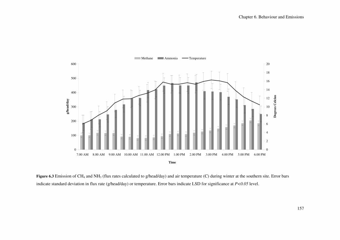
Chapter 6. Behaviour and Emissions
157
0
100
200
300
400
500
600
7.00 AM 8.00 AM 9.00 AM 10.00 AM 11.00 AM 12.00 PM 1.00 PM 2.00 PM 3.00 PM 4.00 PM 5.00 PM 6.00 PM
Time
g/h
ead
/da
y
0
2
4
6
8
10
12
14
16
18
20
Deg
rees
Cel
ciu
s
Methane Ammonia Temperature
Figure 6.3 Emission of CH4 and NH3 (flux rates calculated to g/head/day) and air temperature (C) during winter at the southern site. Error bars
indicate standard deviation in flux rate (g/head/day) or temperature. Error bars indicate LSD for significance at P<0.05 level.

Chapter 6. Behaviour and Emissions
158
0
20
40
60
80
100
120
140
160
180
7.00 AM 8.00 AM 9.00 AM 10.00 AM 11.00 AM 12.00 PM 1.00 PM 2.00 PM 3.00 PM 4.00 PM 5.00 PM 6.00 PM
Time
Nu
mb
er o
f H
ead
Feeding Ruminating
Figure 6.4 Number of cattle feeding and ruminating over 12 hours during winter at the Southern Site. Error bars indicate LSD for significance at
P<0.05 level.

Chapter 6. Behaviour and Emissions
159
6.3.3. Northern Site- Summer 2008
Due to the filtering criteria applied to flux data, CH4 fluxes were calculated for only 48% of
the observed time period (6 am to 6 pm). NH3 fluxes were calculated for 64% of the observed
time period. Fluxes of both CH4 and NH3 (Figure 6.5) were not significantly (P>0.05)
different between time periods. CH4 was highest during the early afternoon (73 g/head/day
and lowest in the late afternoon (43 g/head/day). NH3 was highest in the early morning (403
g/head/day) decreasing to 281 g/head/day in the late afternoon. However the limited flux data
available for this period makes it difficult to examine possible diurnal patterns (Figure 6.5).
Temperature was significantly (P<0.001) higher during the late morning and early afternoon
(26.5 and 26.9 °C). Neither number feeding or ruminating (Figure 6.6) were significantly
(P>0.05) different between time periods. Number feeding tended to be highest in the late
afternoon and lowest in the late morning and early afternoon when temperatures where
highest.
In general, there were no strong correlations (Table 6.3) between emissions of CH4 and NH3
and behavioural parameters. Methane was moderately (but significantly) correlated with NH3
(0.63, P<0.05), but this is likely to be due to the limited data set available. Number feeding
was strongly negatively correlated with temperature (-0.83, P<0.001).
Table 6.3 Correlation matrix (and t-probabilities), for animal behaviour and greenhouse gas
fluxes measured at the Northern Site during summer 2008
Temperature CH4 NH3 Feeding Ruminating
Temperature 1.00 - - - -
CH4 -0.34 NS 1.00 - - -
NH3 -0.36 NS 0.63* 1.00 - -
Feeding -0.83*** 0.38 NS 0.34 NS 1.00 -
Ruminating -0.28 NS 0.38 NS 0.08 NS 0.02 NS 1.00
NSNot Significant, * P<0.05, **P<0.01, ***
P<0.001

Chapter 6. Behaviour and Emissions
160
0
100
200
300
400
500
600
700
800
900
6.00 AM 7.00 AM 8.00 AM 9.00 AM 10.00 AM 11.00 AM 12.00 PM 1.00 PM 2.00 PM 3.00 PM 4.00 PM 5.00 PM 6.00 PM
Time
g/h
ead
/da
y
0.0
5.0
10.0
15.0
20.0
25.0
30.0
35.0
Deg
rees
Cel
ciu
s
Methane Ammonia Temperature
Figure 6.5 Emission of CH4 and NH3 (flux rates calculated to g/head/day) and air temperature (°C) during summer at the northern site. Error bars
indicate LSD for significance at P<0.05 level.
Chapter 6. Behaviour and Emissions
161
0
20
40
60
80
100
120
140
6.00 AM 7.00 AM 8.00 AM 9.00 AM 10.00 AM 11.00 AM 12.00 PM 1.00 PM 2.00 PM 3.00 PM 4.00 PM 5.00 PM 6.00 PM
Time
Nu
mb
er o
f H
ead
Feeding Ruminating
Figure 6.6 Number of cattle feeding and ruminating over 12 hours during summer at the Northern Site. Error bars indicate LSD for significance at
P<0.05 level.

Chapter 6. Behaviour and Emissions
162
6.3.4 Southern Site- Summer 2008
Methane emissions from the Southern Site during summer demonstrate a small peak during
the morning, and increase from midday (Figure 6.7). Methane flux was significantly
(P<0.001) higher during the late afternoon (93 g/head/day) and lowest during late morning
(63 g/head/day). Ammonia flux increased, reaching a peak around midday and decreasing
towards evening. Significantly differences in NH3 flux were observed between time periods,
peaking in the early afternoon (173 g/head/day). At the Southern Site, during summer,
number feeding exhibits a peak in the early morning, and again in the mid to late afternoon
(Figure 6.8). Number ruminating exhibits less distinct peaks in the late morning and the late
afternoon. Number feeding and ruminating did not significantly (P>0.05) vary by time of day.
Emissions of both CH4 and NH3 were not strongly correlated with animal behaviour during
summer at the Southern Site (Table 6.4).
Table 6.4 Correlation matrix (and t-probabilities), for animal behaviour and greenhouse gas
fluxes measured at the Southern Site during summer
Temperature CH4 NH3 Feeding Ruminating
Temperature 1.00 - - - -
CH4 0.18* 1.00 - - -
NH3 0.02 NS 0.32** 1.00 - -
Feeding 0.29 NS 0.17 NS 0.05 NS 1.00 -
Ruminating -0.34 NS -0.12 NS 0.36 NS -0.60** 1.00
NSNot Significant, * P<0.05, **P<0.01, ***
P<0.001

Chapter 6. Behaviour and Emissions
163
0
50
100
150
200
250
6.00 AM 7.00 AM 8.00 AM 9.00 AM 10.00 AM 11.00 AM 12.00 PM 1.00 PM 2.00 PM 3.00 PM 4.00 PM 5.00 PM 6.00 PM
Time
g/h
ead
/day
0
5
10
15
20
25
30
Deg
rees
Cel
ciu
s
Methane Ammonia Temperature
Figure 6.7 Emission of CH4 and NH3 (flux rates calculated to g/head/day) and air temperature (°C) during summer at the southern site. Error bars
indicate LSD. for significance at P<0.05 level.

Chapter 6. Behaviour and Emissions
164
0
20
40
60
80
100
120
140
160
180
200
6.00 AM 7.00 AM 8.00 AM 9.00 AM 10.00 AM 11.00 AM 12.00 PM 1.00 PM 2.00 PM 3.00 PM 4.00 PM 5.00 PM 6.00 PM
Time
Nu
mb
er o
f H
ead
Feeding Ruminating
Figure 6.8 Number of cattle feeding and ruminating over 12 hours during summer at the Southern Site. Error bars indicate LSD. for significance at
P<0.05 level.

Chapter 6. Behaviour and Emissions
165
6.5 Discussion
Anecdotal evidence suggests that greenhouse gas fluxes (CH4 and NH3) from grazing and lot
fed livestock (sheep and cattle) are associated with animal behavioural patterns (Flesch et al.
2007; Lockyer 1997; Loh et al. 2008). From the two feedlots measured, stronger
relationships between behaviour and emissions were observed during winter, than during
summer, when poor correlations were observed. Distinct diurnal patterns were observed for
NH3 emissions, and were consistent between sites and seasons. In contrast, CH4 emissions
exhibited much more variable daily patterns. Environmental conditions are likely to have
contributed both to the different flux patterns observed between summer and winter, and the
changes in animal feeding behaviour.
6.5.1 Cattle Behaviour
Animal feeding behaviour was more different between seasons than between sites. The
delivery of fresh feed has been found to be a stimulant of feeding behaviour in housed dairy
cattle, and feedlot cattle (DeVries et al. 2003; Fell and Clarke 1993). During winter at the
Northern Site, number of cattle feeding increased rapidly following feed delivery, and
continued at a similar level during the afternoon. Similarly, at the Southern Site number of
cattle feeding also increased following the delivery of fresh feed. In winter number feeding
peaked at around 2 pm, and then decreased back to similar levels to the early morning by the
time observations concluded at 6 pm. However, in summer (at both sites) feeding behaviour
exhibits two distinct peaks associated with the early morning and late afternoon. Ray and
Roubicek (1971) noted two distinct peaks of eating activity, cattle started eating around
sunrise, but feeding ceased by mid morning. They noted that the major period of consumption
occurred in the afternoon and early evening. These two peaks were more pronounced during
summer than in winter. Ray and Roubicek (1971) also noted that eating between 6pm and
midnight was increased in steers during summer. Two distinct peaks of feeding activity were
also noted by Gonyou and Stricklin (1981) who also observed a lesser peak during the night
and by Hoffman and Self (1973). Gonyou and Stricklin (1981) noted that feeding behaviour
appeared to be associated with sunrise and sunset and relatively independent of feed
management. These observations are consistent with the summer observations of this study.
It appears environmental conditions and heat load have a significant effect on the feeding
behaviour of feedlot cattle (Castaneda et al. 2004). During winter, when air temperatures are
moderate, timing of feed delivery during the late morning stimulates feeding. During summer,
cattle choose to feed during periods of cooler air temperature. In winter, the highest
frequency of number eating appears to be associated with the time the feed in placed in the

Chapter 6. Behaviour and Emissions
166
bunk however in summer, placing feed in the bunk during the afternoon does not appear to
illicit a response (Ray and Roubicek 1971). We would therefore expect that there would be a
difference in diurnal emissions pattern, particularly of CH4, between summer and winter.
6.5.2 Fluxes
Over the periods observed, both within day and within season, a distinct diurnal pattern was
observed for NH3 flux. Fluxes of NH3 increased from the early morning, peaking during the
early afternoon, NH3 fluxes were significantly different between time periods (excluding the
Northern Site summer 2008). The diurnal pattern of NH3 emissions recorded here are similar
to those reported by Flesch et al. (2007) and Loh et al. (2008). At each site NH3 flux peaked
during the early afternoon, despite a significantly higher magnitude of emissions during
winter at the Southern Site. Methane fluxes were more variable; however (excluding the
Northern Site summer 2008) fluxes were consistently significantly (P<0.05) different
between time of day, tending to be lowest during the late morning, and highest during the late
afternoon. However the timing of depressions and peaks is more variable than the consistency
observed for NH3. The variably of daily emission patterns for CH4 is consistent with the
results of Lockyer (1997) who observed very different patterns, particularly in the period
between sunset and sunrise. However, Lockyer (1997) observed a tendency for CH4 emissions
to increase towards sunset, similar to the observations reported here.
6.5.3 Correlations
Ammonia emissions follow a consistent diurnal pattern at both sites and in both seasons. The
same pattern is reported by a number of other sources- including (Flesch et al. 2007).
Although there appears to be an association between number feeding and NH3 during the
Winter measurement campaigns, this relationship is likely to be primarily due to the
association of both emissions and feeding behaviour with temperature and the timing of feed
delivery. During winter, feed delivery stimulates feeding, which continues throughout the
afternoon, this coincides with the peak in NH3 emissions (and temperature). During summer,
feed delivery does not stimulate feeding to the same extent (behaviour is affected by
temperature). Despite these differences in feeding behaviour, the diurnal pattern of NH3
emissions is consistent between seasons and sites. For all seasons the highest correlation is
observed between temperature and NH3 emissions. As reported by Van Haarken et al (2008) a
24 hour pattern exists for NH3, but this is not closely related to the feeding schedule (for all
seasons). They attribute this to the fact that emissions of NH3 are not a direct animal process.
These results suggest that in contrast to the suggestion of Flesch et al. (2007) and Loh et al.
(2008) who suggest that the increase in emissions is associated with increased animal activity
Chapter 6. Behaviour and Emissions
167
and decreases with decreasing activity in the afternoon. Flesch et al. (2007) suggest that time
of day is the predominant determinant of NH3, as the pattern is consistent (with some
modulation with temperature and wind speed) between days and seasons. The observation
that time of day is the predominant determinant of NH3 is supported by the low correlation
between temperature and NH3 emissions during summer at the Southern Site, despite NH3
flux maintaining a similar diurnal pattern to winter measurements. However, the lack of
animal activity during the early afternoon during these summer measurements suggests that
environmental conditions are more likely to be the primary determinant of diurnal patterns of
NH3 emissions.
The low correlations between emissions of CH4 and rumination are unexpected. Increased
number of animals ruminating (and therefore releasing CH4 via eructation) would be expected
to be associated with increased emissions. However, moderately negative correlations were
observed between CH4 emission and number ruminating during winter at both sites, and a
weak negative correlation at the Southern Site during summer. In general, a positive
correlation was observed between CH4 flux and number feeding. The correlation between
CH4 and number feeding during winter (CH4 increasing with feeding) is consistent with the
observations of Lockyer (1997) and Murray et al. (1999); this was attributed by both authors
to accumulation of ingesta into the rumen and displacement of CH4 with the introduction of
feed material. Murray et al. (1999) also observed that an increase in ruminating (or idling)
after sunset, as the majority of feeding occurs during daylight hours, was associated with a
decrease in emissions (as rumen contents decreased). This observation would be consistent
with the lowest measured emissions occurring just prior to feed delivery.
6.5.4 Other Considerations
Behavioural observations were not able to be conducted over night; therefore definite
conclusions cannot be drawn about the patterns of emissions during this period. However, in
both winter and summer emissions tend to peak in the early evening (slightly later in
summer). During winter these emissions drop back to “daytime” levels over night, however in
summer emissions continue to be high until the early morning. Although, based on the results
of this study, this is unlikely to be related directly to feeding behaviour it is possible that
alterations in the timing of feeding bouts associated with seasonal differences in temperature
and photoperiod may be contributing to these differences. Gonyou and Stricklin (1984)
observed a significant period of feeding near midnight during winter in lot fed cattle, however
this decreased in duration (and intensity) as photoperiod increased. The longer day length in
summer will have resulted in delayed timing of the feeding bout associated with sunset. This
Chapter 6. Behaviour and Emissions
168
would potentially increase emissions during the early evening, but is unlikely to explain the
maintenance of higher emissions until early morning.
However, the increase in CH4 emissions during the late afternoon and evening may also be
related to micrometeorological conditions. When using micrometeorological measurements, a
commonly observed phenomenon is a period of atmospheric boundary layer stability after
sunset (low turbulence and wind movement; Griffith et al. 2002). These results in
concentration build up under the inversion layer, and can result in very low accuracy in
calculations of fluxes using dispersion modelling (Flesch et al. 2007). Laubach and Kelliher
(2004) examined concentrations and CH4 emissions estimates from various periods over the
day (measured using micrometeorological methods) and determined increased concentrations
(from 250 g/head/day to 400 g/head/day) associated with the change from unstable day
conditions to stable night time conditions. This trend appears to be more clearly demonstrated
during summer than winter (see appendix), and is potentially associated with differences in
environmental conditions, such as wind speed and turbulence. Yi et al. (2001) report that the
boundary layer is often not clearly defined during heavy cloud or rainfall, and demonstrates
differences between the height of the stable boundary layer between seasons. Similarly,
Dayan and Rodnizki (1999) observed the depth and frequency (of occurrence) of the
boundary layer to be greater in summer. Both these factors are possible explanations for the
differences in “over night” emissions patterns between seasons.
This is additionally a potential source of the diurnal emissions pattern observed for NH3.
Temperature and air inversion create a boundary layer, which may hold NH3 near the surface
over night reducing volatile NH3 in the atmosphere until air temperature warms and more
turbulence is created by less stable conditions. Further, high concentrations of NH3 near the
surface of the manure pad will impact rate of diffusion of NH3 from the manure pad to the
atmosphere. However further examination would be required to draw conclusions about
sources of diurnal variation in NH3 emissions.
Errors associated with this methodology (as evidenced by the reduction in flux data from the
Northern summer campaign) may influence reported diurnal patterns as well as average
emissions estimates. Further, although video recording and assessment of behaviour at ten to
30 minute intervals has been found to be relatively accurate for longer term behaviours (Hao
et al. 2001a). However, short term behaviours may not be observed. Additionally, video
recording techniques are commonly used for housed animals. Although feedlot animals are
confined to a relatively small area the placement of the camera resulted in incomplete
coverage of the pens (roughly 95% of the pens could be seen on the video at any time). The

Chapter 6. Behaviour and Emissions
169
ability to easily distinguish between idling and ruminating cattle in the video recording was
limited at times. Further development of the methodology, perhaps utilising smaller numbers
of cattle and smaller areas in an artificial feed yard situation may enable increased ability to
draw conclusions.
6.6 Conclusion
Diurnal pattern of NH3 emissions is more strongly associated with environmental conditions
than animal activity, as evidenced by the similarity in emissions despite seasonal differences
in animal feeding behaviour. In contrast, CH4 emissions are more closely associated with
feeding behaviour (increases in number feeding) than ruminating; however the correlation is
greater in summer than winter. Feeding behaviour explains only a small amount of observed
diurnal patterns of emissions. If “snap-shot” sampling methods are going to be utilised,
consideration needs to be given to changes in emissions with time of day. When unfavourable
wind conditions result in limited data points which can be used in the estimation of emissions,
calculated values may be significantly impacted by the time of day in which these data points
are centred. Clustering of usable data in periods of high or low emissions may result in
artificial inflation/deflation of daily average emissions. This is potentially a significant
limiting factor for the use of micrometeorological methods over short term measurement
campaigns.

Chapter 7. General Discussion
170
Chapter 7. General Discussion
7.1. Introduction
This thesis examined greenhouse gas emissions from beef feedlot operations in Australia,
including investigating differences in magnitude of emissions between sites and seasons, role
of intake behaviour in influencing diurnal emissions fluctuations and the application of a
modelling methodology for prediction of emissions. But why are emissions from feedlot
systems important or different from other livestock production systems? Why do we need to
account for emissions, and what is the role of predictive equations?
In this Chapter the research findings are contextualised in the current and future policy
situation regarding greenhouse emissions from agricultural systems and from high to low
level; in order to address the above questions. Opportunities for mitigation and quantification
of emissions are outlined and areas for future exploration in modelling approaches discussed.
7.2 Feedlot Production
The principle of feedlot operation is the ability to produce a consistent product efficiently.
Although the majority of Australian beef production occurs on pasture (particularly at the
breeding, cow/calf pre finishing stages) cattle are being increasingly finished using feedlot
operations in response to consumer demand. The ability to control quality and quantity of
finished cattle throughout the year and produce faster growth rates and finishing makes
feedlot operations very efficient (Charmley et al. 2008; Pritchard 2006; Stackhouse et al.
2011). Approximately 65% of Australian beef is exported annually, although domestic
production is still the largest single market (ALFA 2008). Another significant output of
feedlot systems is nutrients (N and phosphorus) and greenhouse gases (CH4, N2O and the
indirect greenhouse gas NH3); which effectively represents an inefficiency or leakage from
the system.
Characteristics of feedlot production mean that the emissions profile is considerably different
to other cattle feeding operations, including grass fed, rangeland and pastoral beef and dairy
systems. The concentrated nature of a feedlot, with large numbers of cattle confined in a
relatively small area makes the site a significant point source of enteric CH4. Built up manure,
in pens, effluent systems and compost piles is a source of CH4, N2O, NH3 and volatile
compounds. A considerable part of the efficiency of feedlot operations results from the ability
to supply rations balanced for energy, protein and other dietary requirements in the quantities

Chapter 7. General Discussion
171
required for growth. Feedlot rations are typically higher grain and higher energy than a
pasture based ration, resulting in not only faster growth rates, but improved efficiency.
In Australian feedlots, cattle are typically fed to meet domestic or export markets (which can
be long or short fed), cattle will be yarded within the feedlot based on breed, age, weight and
likely market. Cattle spend between 50 and 120 days on average in a feedlot, dependent on
market. The concentrated nature of feedlot operations results in a build up of manure, which,
like an individual dung or urine patch, can provide a significant source of CH4, N2O and NH3.
However, emissions from the manure pad differ from those from a single dung pat or urine
patch due to built up manure and manure of varying ages (Miller and Berry 2005; Miller et al.
2003; Stackhouse et al. 2011).
Additionally, feedlot rations differ from grazing systems with the addition of products (e.g.
oils, rumen modifiers) which are commonly reported to reduce emissions, and proposed as
mitigation options. These options can be applied more easily under the controlled feeding
environment of the feedlot, where feed is provided daily, than in a grazing (intensive or
extensive) system. Lipid based supplements (commonly recycled vegetable oil) are
commonly utilised in feedlot rations, which may contribute to lower emissions. However,
there may be limited potential for further emissions reduction, due to the higher basal
efficiency of the system (compared with grazing operations).
There may also be some differences in the feeding behaviour of feedlot cattle, particularly in
winter where timing of feed delivery has a greater impact on timing of feeding (number of
cattle feeding immediately following feed delivery declines sharply in summer, but remains
higher during winter). However, similar to grazing systems, feedlot cattle demonstrate feeding
bouts near sunrise and sunset in both seasons. However, this may influence diurnal emissions
profile in relation to a grazing animal, and have implications for snapshot measurements of
enteric emissions, and for micrometeorological measurements, where large amounts of data
can be filtered based on environmental conditions.
7.3 The Need for Accounting
Quantification of emissions from feedlot systems is necessary due to requirements for
national auditing and reporting of emissions, under the Kyoto Protocol and international
agreements (administered by the IPCC) and for use in a potential emissions trading scheme.
Despite the current debate around the application of a Carbon Tax and/or price for carbon
credits in Australia, consensus has been to exclude Agriculture from a direct Carbon Tax in
the immediate future, although the Carbon Farming Initiative will allow agricultural

Chapter 7. General Discussion
172
producers to utilise mitigation practices to generate carbon credits. There is increasing public
awareness and demand for low emissions, low pollution products, which is likely to continue
in the future.
The increased requirement for accounting due to government requirements notwithstanding,
accurate accounting for emissions may be a useful tool in benchmarking the efficiency of the
system in terms of energy and protein use. CH4 is a loss of energy, which could potentially be
utilised as energy for growth or production (although there is little concrete evidence that
decreasing CH4 emissions increases growth or milk production). Whilst N/protein is
commonly one of the most expensive ingredients in feeds, and often slightly overfed (to avoid
limitations to growth). High levels of N, in excess of requirements, result in the animal
expending energy to process the excess as well as excretion of significant quantities of N. The
ability to accurately account for emissions could have significant benefits for operators in
terms of examining potential changes to their production system.
7.3.1 Measurement as an Accounting Method
The ideal way of accounting for emissions is direct measurement. Measurements of enteric
CH4 were originally undertaken using calorimetric methods, in order to examine the loss of
feed energy from CH4. Calorimetric approaches continue to be used for experimental
purposes; however they have limited applicability under commercial conditions due to
requirements for enclosure of animals (and availability of appropriate calorimetric facilities).
Traditional measurements of nitrogenous gases has utilised chamber measurements, static or
dynamic, or various sizes. These chambers are used to contain subsamples of manure/ soil,
placed over artificial feed yard surfaces, or for in situ measurements. More recently
techniques which enable animals to remain under grazing/ unrestrained, the SF6 technique and
measurement using tuneable diode lasers (or similar) accompanied by calculations based on
wind statistics (commonly known as micrometeorological methods).
It can be considered that the primary difference between measurement approaches is between
measurement of individual components or the whole system. The application of component
measurement methods, such as calorimetry and SF6 under commercial situation is impractical,
given the requirements for infrastructure, training of animals, and in the case of SF6 dosing
with a sulfar-hexaflouride bolus, which has a withholding period prohibitive for commercial
meat production. The use of small chambers and short term measurements for nitrogenous
gases can result in inability to capture spatial and temporal variation which can significantly
impact on estimated emissions. For NH3 volatilisation, due to its nature and reversible
physical-chemical process, micrometeorological techniques, are needed to measure losses

Chapter 7. General Discussion
173
from the whole system. From this perspective, whole of system approaches which can provide
indirect measurements (limiting impacts on animal behaviour and intake and encompassing
spatial variability within soil or manure) should enable more accurate accounting.
Although not a primary aim of this thesis, the use of micrometeorological measurements in
the comparison between modelled and measured emissions highlighted one of the major
issues with micrometeorological measurements- the loss of useable observations under
unfavourable environmental conditions. In contrast to a calorimetric chamber, where
conditions are closely controlled, micrometeorological measurements rely on wind speed,
direction and turbulence to be between set parameters to enable accurate estimation of
emissions from measured concentration. This effect is demonstrated clearly in the comparison
between the numbers of data points used in the calculation of average emissions from the
Northern Site summer 2008 measurement campaign, with the remainder of the campaigns.
The reduced data points resulted in much more variable average emissions (SE is more than
20 times higher) for all reported gases, making it difficult to draw conclusions when
attempting to quantify emissions. Increased variability in measurement using these types of
approaches may also make the assessment of mitigation options difficult. Where expected
reductions are less than the variability observed, it may be difficult to determine either a
statistically or practically significant value. However, this approach remains the most viable
for measuring whole system emissions, provided the limitations are understood.
The effect of reduction in useable data under unfavourable environmental conditions is
compounded when emissions show a distinct diurnal pattern. Although this study
demonstrated low correlations between animal behaviour and emissions there was observed to
be a distinct diurnal pattern in emissions of both NH3 and CH4. The pattern of NH3 emissions
was more consistent between seasons and sites, but CH4 was more variable. The variation in
CH4 emission could potentially be associated with differences in feeding times due to climatic
conditions and timing of feed delivery. However, where the usable data points are clustered
around periods of peaks or troughs in emission (as they were during the Northern Summer
2008 campaign) artificial inflation or deflation of average emissions can occur.
Although measurements of emissions from agricultural systems would enable accurate
inventories the cost can be prohibitive. Further, the challenges associated with all
measurement methods makes application difficult, particularly under commercial situations
where value for money (in terms of accurate emissions obtained for investment in
measurement equipment/ expertise) is likely to be as important to the enterprise as obtaining
accurate estimates of emissions.

Chapter 7. General Discussion
174
7.3.2 Modelled Emissions Estimates for Accounting
The impracticality of direct measurement of emissions from each individual feedlot operator
means an indirect method of estimating emissions is required for accounting purposes. A
standard methodology is prescribed by the IPCC (for various industries); however, where
agriculture is a key source category (such as Australian and New Zealand) the use of a
country specific methodology is recommended. For feedlot cattle in Australia, CH4 estimates
are based on the equation developed by (Moe and Tyrrell 1979) and on volatile solid
excretion (combined with a country specific manure CH4 emissions factor). Emissions of
nitrogenous gases are predicted utilising an N excretion estimate based on SCA guidelines
and country specific emission factors (for N2O and NH3). A similar approach is taken for N
emissions under IPCC guidelines, and the same emissions factors are used in both the IPCC
and Australian methodologies.
A key aspect of the evaluation was to examine the ability to utilise data available from
commercial feedlot operations, reducing requirement for additional recording for accounting
purposes. Feedlot cattle are managed primarily on a pen or lot basis, weights are estimated on
arrival based on the weight of the transport vehicle and number of cattle, feed is delivered and
rationed on a pen basis and growth is estimated by a pen basis. There appears to be a
difference in the reliability of emissions estimates between individually measured values and
measured values from the whole system. The more detailed CHO based equations Moe and
Tyrrell (1979) and Ellis et al. (2007) show a closer relationship to emissions measured on an
individual basis, presumably due to increased specificity compared with the Tier II approach.
However, for emissions measurements based on the whole feedlot the Tier II approached
showed (overall) the closest relationship between measured and predicted emissions.
However, over-estimation with the CHO equations and under estimation with the Tier II
equation was consistent between published and measured data (Chapters 4 and 5). In terms of
Tier II, this is likely to be due to the range of grain concentrations observed in feedlot rations,
which can limit the applicability of a single emissions factor. Kebreab et al. (2006) suggests
that with ration specific emission factors the Tier II equation may provide reasonable
estimates of emissions. Although this equation demonstrated the closest relationship (overall)
with measured emissions the differences observed in accuracy between sites and seasons
suggest that it needs to be modified in order to improve emissions estimates.
An issue with all the current approaches for estimating enteric CH4 is that despite the ability
of the CHO based equations to account for differences in ration composition, there is limited
ability to account for the use of mitigation options, such as lipids or dietary additives. In

Chapter 7. General Discussion
175
Chapter 4, an equation developed by Ellis et al. (2009) which included fat as a parameter was
evaluated; however accuracy proved to be reduced compared with the other options. Future
accounting methodologies need to be not only accurate, but able to account for reductions
associated with mitigation. It is clear further development is required if an empirical
modelling approach is to be used in preference to a dynamic/ rumen simulating approach.
The failure of predictive approaches for N (NH3 and N2O) gas emissions is due in the most
part to the lack of consideration of the impact of environmental conditions on emissions.
Emissions of nitrogenous gas from the manure pad is influenced not only by quantities of N
excreted and the form of N (urine or faeces) of the current cattle, which is accounted for in the
modelling approach, but accumulated manure, substrate pH, moisture content, organic matter
and temperature. However, it should be noted that the measurement campaigns reported here
and used in the application of the model are short term measurements. It is possible that the N
emissions factors (0.3 for NH3 and 0.02 for N2O) may be appropriate when considered
annually (or over the time which an individual pen of animals spend on feed), although they
are inaccurate for short term measurements.
7.4 Implication of Inaccurate Accounting
This thesis demonstrates that there are issues with over estimation of both enteric (and manure
pad) CH4 and N2O, and underestimation of NH3 under the current National Inventory
approach (AGO 2006). Despite agriculture being excluded from a Carbon Trading scheme
indefinitely, there will still be pressure on agricultural industries (political and social) to
produce low emissions products. However, this will need to occur within a carbon constrained
economy. The RIRDC (Jiang et al.2009) recently examined the impact of an emissions
trading scheme on agricultural industries, under 2 prices for carbon ($25 and $50/ tonne), and
scenarios of full agricultural inclusion and indirect impacts (agriculture not included). Key
aspects of the analysis which may impact the productivity of feedlot operations included a
projected increased in the cost of purchasing cattle of between 1.28 and 2.35 % for a full
inclusion scenario (at $25 and $50/ tonne respectively) or 0.13 and 0.25% for a non inclusion
scenario. They determined the primary increase in cost to be related to the introduction of
abatement methods, or purchase of permits. Under a full inclusion scenario a beef farm is
suggested to have the biggest fall in farm income under both carbon prices (63 and 125%
respectively), compared to grain, sheep, horticulture and mixed farming. Under a non
inclusion scenario, agricultural industries would still be affected due to changes in prices of
inputs including fuel, fertiliser, transport and other goods and services. The RIRDC (Jiang et
al. 2009.) suggest that the cash income of a beef operation would decrease by 2.7% under a
Chapter 7. General Discussion
176
non-inclusion scenario. The impacts of increased costs of fuel and transport would be likely to
have a greater impact on a feedlot operation than an extensive beef operation, given the high
proportion of fuel and transport costs in operating costs.
Over-estimation of emissions will increase the pressure to reduce emissions, substantially
easier to achieve actual reductions. Under estimation of emissions will actually make it harder
to achieve actual reductions, whilst will not encourage the application of mitigation practices,
or changes to current practice, particularly if this adds an additional cost to the system.
7.5 Opportunities
The nature of the feedlot system means that application of mitigation strategies (such as lipids
and rumen modifying additives) can be easily utilised in the production system; indeed lipids
and fats as well as additives are commonly already added to feedlot rations to increase energy
density. This thesis does not aim to fully explore mitigation options; however the need to
include reductions in emissions associated with the use of mitigation options in
methodologies should be highlighted.
Of equal importance to the reduction of emissions is accurate accounting for emissions from
the system. As described, the cost of measurements using calorimetric and
micrometeorological methods can limit use under commercial conditions. This results in short
term measurement periods, limiting the ability to evaluate emissions over whole growth
periods and examine seasonal differences. Denmead et al. (2008) report on emissions
measured using a fixed trace gas station (Ecotech Pty Ltd), which utilises a point
measurement rather than a path length measurement of concentration. The benefit of this
approach is that once set up, the unit can be left in place for long periods enabling long term
measurements and assessment of changes in emissions. The unit utilised by (Denmead et al.
2008) contained a CH4/non CH4 hydrocarbon analyser, an NH3 chemiluminescence analyser
and a NO/NO2/NOx chemiluminescence analyser allowing measurement of the greenhouse
gas of interest. As with other micrometeorological measurements, this equipment is expensive
and requires some expertise to apply and use correctly. However, this may provide a tool for
researchers to monitor long term emissions and correlate these with animal production,
rations and climatic conditions. This is particularly relevant for measurements of the
nitrogenous gases, as long term measurements with automatic dynamic chambers are
impractical in occupied pens. New high sensitivity, low maintenance and more reliable
sensors are emerging which will make long term measurement more feasible.

Chapter 7. General Discussion
177
More precise measurement of enteric CH4 can be obtained from direct measurements of
rumen gas production; however this is difficult without the use of fistulated cows in an
intensively managed situation. More recently wireless sensors (boluses) have been utilised in
ruminant nutrition, measuring pH, temperature and pressure telemetrically and in real time
(Laporte-Uribe et al. 2010) and can be used in non fistulated cattle (Lin 2009). Lin (2009)
evaluated the Kahne bolus (which is commercially available) for effectiveness in monitoring
rumen pH under both indoor and outdoor feeding situations and determined they were
effective. They also discuss the use of a pressure sensing bolus for measurement of changes in
rumen pressure (Lin 2009). Rumen boluses which measure pH are commercially available in
New Zealand (Kahne Ltd) and the United Kingdom (WellCowTM) targeted at primarily dairy
farmers for the management of subclinical acidosis, however with further development they
may have application for CH4 production. The recording span of the bolus is up to 100 days
(WellCowLtd 2009), making it suitable for monitoring cattle over the finishing period in a
feedlot.
Montanholi et al. (2008) draw on the concept that more efficient dairy cattle demonstrate both
lower heat loss and lower CH4 production and examined the use of infrared thermography
(which has also seen recent evaluation in heat stress research) in prediction of CH4
production. Infra-red measurements of the difference in temperature between the left and right
flank showed correlations of between 0.53 and 0.77 dependent on time of day (time following
feeding). In the periods after feeding temperature difference explained 60% of the variation in
CH4 emissions. This approach would be non-invasive, relatively inexpensive and easily
applied, which would enable easy adoption under commercial feedlot operations. However,
significant further research and demonstration of effectiveness is required before it could be
applied to large numbers of cattle or for the purposes of accounting.
For a feedlot system, where the majority of “measurements” are conducted on a pen basis
(estimates of weight, intakes) modelling emissions on a pen basis (whilst still accounting for
the potential variability between individual animals) would have more relevance in terms of
the production system. Further, drawing links between cattle class and emissions would
provide a useful tool in terms of accounting. Within the feedlot system cattle are fed for a
specific market (generally domestic, short fed export or long fed export). If a greenhouse gas
emission value could be applied to each of these classes numbers in each category reaching
the processor (detailed are reported back to the feedlot) could be used as a proxy for detailed
inventory calculations. The increase in accuracy in the validation study (Chapter 4) for the
carbohydrate based equations when using the class-based-intake rather than the measured
intake indicates the possibility for further development in this area.

Chapter 7. General Discussion
178
7.6 Implications
This study highlights the contributions of the various gases to total feedlot emissions. In
contrast to expectations, feedlot emissions are dominated by nitrogenous gases, in the form of
NH3, rather than CH4. Based on the feedlots measured, an “average” feedlot steer in a feedlot
is predicted to emit 183 g CH4, 62 g NH3 and 6.5 g N2O daily. However measured emissions
reported here and by Chen et al. (2009) indicate CH4 emissions closer to 119 g/head/day (94.0
to 130.3), NH3 emissions closer to 154 g/head/day (94 to 305 g/head/day) and N2O emissions
of 3 g/head/day (0.1 to 5.7 g/head/day). On an individual site basis (Northern Australian
feedlot compared with Southern) an average animal (and manure contribution) at the Northern
Site is predicted to emit 187 CH4, 62 g NH3 and 6.5 g N2O daily, whilst measured emissions
from this site suggest each animal contributes 132 g CH4, 123 g NH3 and 3.6 g N2O. From the
Southern Site, predicted emissions were 181 g CH4, 61.2 g NH3 and 6.4 g N2O per head daily.
Whereas measured emissions are closer to 110 g CH4, 178 g NH3 and 2.6 g N2O. From both
sites, NH3 volatilisation is considerable higher than predicted, however daily emissions of
CH4 and NH3 are more similar from the Northern Site (132 and 123 g/head/day) compared
with the Southern Site, where emissions of NH3 are considerably higher than CH4 (178 and
110 g/head/day).
Denmead et al. (2008) assumed potential emissions of indirect N2O from deposition of NH3 to
be equal in magnitude to direct N2O, amounting to approximately 3 g/head/day. Using the
same approach as (Denmead et al. 2008) indirect N2O is calculated at 1.25% of deposited N,
and that all NH3 is assumed to be deposited, measured emissions of NH3 account for an extra
1.9 g indirect N2O/head/day. Nitrogen is predicted to contribute an average of 40% of total
CO2-e and up to 52% of total CO2-e (predicted contribution range from 34 to 39% total CO2-
e). Based on average values, the contribution of N to total emissions is slightly greater at the
Northern Site (where NH3 emissions are included as indirect N2O). N gases contribute 40% to
total CO2-e at the Northern Site, compared with 39% at the Southern Site. This similarity
arises from the higher direct N2O loss measured at the Northern Site, resulting in 1.8
kg/head/day CO2-e from N and 2.8 kg/head/day from CH4. At the Southern Site, the lower
direct N2O emissions (2.6 g/head/day) and indirect N2O (from NH3) contribute 1.4
kg/head/day CO2-e, whilst CH4 contributes 2.3 kg/head/day to total CO2-e.
Although not a considerable difference in terms of contribution of CO2-e, the higher NH3
emissions on a daily basis recorded at both sites, but in particular at the Southern Site,
indicate that mitigation strategies should be evaluated and applied not only for CH4 emissions.
This contribution of N to total emissions demonstrates that whilst mitigation strategies could

Chapter 7. General Discussion
179
be applied effectively to CH4, between 40 and 50% of total CO2-e is contributed by N, and a
substantial amount of this through indirect emissions of N2O, coming from NH3. Therefore
management strategies to reduce excess N excretion and volatilisation could have a
significant impact on total CO2-e emissions from feedlots. However, this is based on the
assumption (Denmead et al. 2008) that all volatile NH3 eventually becomes a source of N2O.
Volatilisation, deposition and potential indirect N2O emissions require further investigation
from concentrated animal feeding operations.
As discussed in the literature review, feeding a high digestibility high grain ration has been
observed to reduce emissions by a number of sources (Beauchemin and McGinn 2005; Boadi
et al. 2004b), additionally additives such as oils and products which modify rumen
fermentation (e.g. monensin) are commonly added to feedlot rations already. The results of
this study demonstrate this impact, particularly when the Southern Site is considered, a
change in grain concentration (averaged over rations offered) of 9% from 61 to 70% grain
was associated with an increase in average CH4 emissions from 95 g/head/day to 125
g/head/day. Although this demonstrates the potential for further reducing emissions feedlot
rations are balanced to produce maximum growth whilst avoid metabolic conditions (sub
clinical and clinical acidosis) which may limit more significant reductions in ration forage
concentration difficult. Although, rations at the Northern Site comprise up to 89% grain, and
Beauchemin and McGinn (2005) fed rations of 90% grain to finishing cattle. Suggesting
further increases in grain concentration are feasible.
Despite rationing systems such as the MP (metabolisable protein system, NRC) enabling
feedlot rations to be formulated so requirements are met but not exceeded (Klopfenstein and
Erickson 2002) and protein being one of the more expensive feed components, over feeding
of protein occurs to avoid limitations in growth (Cole et al. 2003). Rations are formulated
with a safety margin increasing concentrations above those required (Vasconcelos et al.
2007). Overfeeding of N (in the form of crude protein) is a significant source of volatile NH3;
protein consumed above requirements is excreted, primarily in the urine, its most volatile
form. The greater emissions of NH3 from the Southern Site may potentially be attributed to
overfeeding protein, which also indicates a simple approach to reducing NH3 volatilisation. At
the Southern Site, CP % in the rations averaged 14 %, compared with 13.5% at the Northern
Site, despite lower live weights (477 kg compared with 598 kg), and lower estimated growth
rates (1.3 compared with 1.8 kg/day). Todd et al. (2006) observed decreasing crude protein
from 13% to 11.5% decreased daily NH3 emissions by 28% (on an annual basis) however
impact on animal performance was not reported. Although they suggest that “reducing crude
protein in beef cattle diets may provide the most practical and cost-effective way to reduce

Chapter 7. General Discussion
180
NH3 emissions from feedyards” (Todd et al. 2006). Similarly Vasconcelos et al. (2006)
determined that reducing CP concentration during the finishing period did not affect feedlot
performance but can reduce the N content of manure. However, environmental conditions and
pen management can also play a considerable role in regulating NH3 volatilisation and further
investigation surrounding (for example) pen cleaning frequency, altering surface pH and the
use of urease inhibitors is required (in association with dietary changes) to effectively
manage NH3 volatilisation (Cole et al. 2005; Todd et al. 2006).
A number of policy solutions for reduction of carbon emissions have been proposed in a last
3-5 years, associated with the end of Kyoto obligations. The initial approach was the Carbon
Pollution Reduction Scheme (CPRS), a cap and trade approach which was intended to effect a
reduction in emissions to 60% of 2000 levels by 2050. This approach was intended to be
applied by mid 2010; however its introduction was deferred early in 2010, in favour of a fixed
carbon price. Due to commence in July 2012, the “Carbon Tax” is a fixed price on C
emissions (initially $23/ tonne) applied to the top 500 polluters, or about 0.02% of Australian
businesses.
The current approach of the Carbon Tax does not include emissions from agriculture,
consistently; the CPRS was not proposed to cover agriculture within the first three years, with
intended inclusion after the 5th year. However, the recently introduced Carbon Farming
Initiative (CFI) will allow agricultural industries to become actively involved in Carbon
Trading (Austalian Government 2010a) and is a further reason why baseline emissions from
feedlots need to be measured. The CFI introduces legislation to establish carbon crediting for
offset/ emissions reduction projects. Effectively, businesses with high emitters can purchase
carbon credits- units of greenhouse gas abatement achieved (in agricultural industries) by
either reducing or avoid emissions, or by removing and storing atmospheric C. This activity
needs to be additional to any management strategy which was undertaken prior to the CFI
(Austalian Government 2010b).
Methodologies for emission reduction, which comprise detail of the implementation of
abatement or mitigation approaches need to also detail how these approaches will be
monitored (Austalian Government 2010a). One of the current submissions (and the only
animal based proposal submitted to date, is reduction of CH4 emissions through the
management (culling) of feral herbivores (camels). In this approach (Australian Government
2010b), baseline emissions are estimated using an empirical equation- effectively derived
from the National Inventory Methodology (2006)). Although camels appear to have little
relevance to feedlot cattle, the approach for estimating baseline emissions using the set of

Chapter 7. General Discussion
181
equations in the current methodology could be transferable to other projects proposed under
the Carbon Farming Initiative. The results of this thesis demonstrate inaccuracies in the
estimation of emissions using these methods, and indicate further measurements are required
for emissions benchmarking before a “business as usual” baseline emission can be
established.
7.7 Conclusion
This thesis examines emissions from Australian beef feedlot systems, diurnal fluctuations in
emissions and the role of animal feeding behaviour in these emissions profiles. The current
Australian National Inventory Methodology (AGO 2006) was evaluated with both published
data and with measurements from Australian beef feedlots.
Although the equations on which the current methodology (for enteric CH4) is based
performed adequately with the results of published studies, it did not demonstrate the same
accuracy when applied to Australian measurements. The results of both the validation
(Chapter 4) and application exercises (Chapter 5) indicate that diet specific calculations will
be essential in the prediction of enteric CH4 emissions. Whether this is a more complex
approach considering dietary CHO, or a simpler modified Tier II approach. The diurnal
pattern of emissions of both CH4 and NH3 is not entirely controlled by behaviour, particularly
in the case of NH3, which is influenced more strongly by environmental temperature (which
in turn influences feeding behaviour). Diurnal fluctuations can influence emissions
measurements using micrometeorological measurements when coupled with poor
environmental conditions, and caution needs to be taken in assessing the results from these
measurement approaches.
The prediction of nitrogenous emissions using a set emissions factor has significant issues,
due to the lack of consideration of the role of environmental conditions in moderating
emissions. A more detailed approach will be required to improve these estimates- including
long term measurements of not just emissions, but animal and ration characteristics and
manure pad composition.
Development of technologies around measurements and increasing social demand for reduced
emissions products will increase both ability to measure emissions on farm, and requirement
to do so. In either case, further research will only increase accuracy of emissions
measurements and enable development of a more reliable model for emissions prediction.

Chapter 8. References
182
Chapter 8. References
Australian Bureau of Agrictulural and Resrouces Economics (ABARE) and Ministry of
Agriculture and Forestry (MAF, NZ), (2006) ‘Agricultural Economics of Australia and New
Zealand.’ (ABARE, Canberra, Australia).
Adams JR, Farran TB, Erickson GE, Klopfenstein TJ, Macken CN, WIlson CB (2004) Effects
of organic matter addition to the pen surface and pen cleaning ferquency on nitrogen mass
balance in open feedlots. Journal of Animal Science 82, 2153- 2163.
AFIC (1987) ‘Australian Feed Composition Tables: National Collection (1970-1987).’
(AFIC-CSIRO, Sydney, Australia).
Australian Greenhouse Office (AGO) (2006)’ Australian Methodology for the Estimation of
Greenhouse Sources and Sinks 2005; Agriculture.’ (Commonwealth of Australia, Canberra,
Australia).
Alford AR, Hegarty RS, Parnell PF, Cacho OJ, Herd RM, Griffith GR (2006) The impact of
breeding to reduce residual feed intake on enteric methane emissions from the Australian beef
industry. Australian Journal of Experimental Agriculture 46, 813-820.
Amon B, Th A, Boxberger J, Ch A (2001) Emissions of NH3, N2O and CH4 from dairy cows
housed in a farmyard manure tying stall (housing, manure storage, manure spreading).
Nutrient Cycling in Agroecosystems 60, 103-113.
Archibeque SL, Freetly HC, Cole NA, Ferrell CL (2007) The influence of oscillating dietary
protein concentrations on finishing cattle. II Nutrient retention and ammonia emissions.
Journal of Animal Science 85, 1496-1503.
Archibeque SL, Miller DN, Freetly HC, Ferrell CL (2006) Feeding high moisture corn instead
of dry-rolled corn reduces odourous compound production in the manure of finishing beef
cattle without decreasing performance. Journal of Animal Science 84, 1767-1777.
Arogo J, Westerman PW, Heber AJ, Robarge WP, Classen JJ (2006) Ammonia emissions
from animal feeding operations. In 'Animal Agriculture and the Environment, National Center
for manure and animal waste management, white papers.' (Eds JM Rice, DF Caldwell and FJ

Chapter 8. References
183
Humenik) pp. 41-88. American Society of Agricultural and Biological Engineers: St Joseph,
MI.
Australian Lot Feeders Association (ALFA) (2008) ‘Response to carobon pollution reduction
scheme green paper’. Public domain submission to the Federal Government, Canberra, 2008.
Austalian Government Department of Climate Change and Energy Efficiency (2010a) Carbon
Farming Initiative. http://www.climatechange.gov.au/cfi. Accessed 15 July 2011.
Austalian Government Department of Climate Change and Energy Efficiency (2010b)
OffsetMethodologies.http://www.climatechange.gov.au/government/initiatives/carbon-
farming-initiative/methodology-development.aspx. Accessed 15 July 2011
Bureau of Agricultural Economics (BAE) (1976) ‘Production Systems in the Australian Beef
Cattle Industry.’ (BAE, Canberra, Australia).
Baek B-H, Todd RW, Cole NA, Koziel JA (2006) Ammonia and hydrogen sulphide flux and
dry deposition velocity estimates using vertical gradient method at a commercial beef cattle
feedlot International Journal of Global Environmental Issues 6(2/3), 189-203.
Baldwin RL (1995) 'Modelling Ruminant Digestion and Metabolism' (Chapman and Hall:
London, UK).
Ball BC, Scott A, Parker JP (1999) Field N2O, CO2 and CH4 fluxes in relation to tillage,
compaction and soil quality in Scotland Soil and Tillage Research 53, 29-39.
Beauchemin KA, McGinn SM (2005) Methane emissions from feedlot cattle fed barley or
corn diets. Journal of Animal Science 83, 653-661.
Beauchemin KA, McGinn SM (2006) Enteric methane emissions from growing beef cattle as
affected by diet and level of intake. Canadian Journal of Animal Science 86, 401- 408.
Bekku Y, Koizumi H, Oikawa T, Iwaki H (1997) Examination of four methods for measuring
soil respiration. Applied Soil Ecology 5, 247-254.

Chapter 8. References
184
Bell MJ, Wall E, Russell G, Simm G Modelling methane output from lactating and dry dairy
cows In 'Aspects of Applied Biology 93, Integrated Agricultural Systems: Methodologies,
Modelling and Measuring', 2009, SAC Edinburgh, UK. (Eds M MacLeod, S Mayne, N
McRobertset al), pp. 47- 53
Benchaar C, Pomar C, Chiquette J (2001) Evaluation of dietary strategies to reduce methane
production in ruminants: a modelling approach. Canadian Journal of Animal Science 81, 563-
574.
Benchaar C, Rivest J, Pomar C, Chiquette J (1998) Prediction of methane production from
dairy cows using existing mechanistic models and regression equations. Journal of Animal
Science 76, 616-627.
Bevans DW, Beauchemin KA, Schwartzkopf-Genswein KS, McKinnon JJ, McAllister TA
(2005) Effect of rapid or gradual grain adaptation on subacute acidosis and feed intake by
feedlot cattle. Journal of Animal Science 83, 1116-1132.
Bierman S, Erickson GE, Klopfenstein TJ, Stock RA, Shain DH (1999) Evaluation of
nitrogen and organic matter balance in the feedlot as affected by level and source of dietary
fiber. Journal of Animal Science 77, 1645-1653.
Bindon BM, Jones NM (2001) Cattle supply, prouction systems and markets for australian
beef. Australian Journal of Experimental Agriculture 41, 861-877.
Blaxter KL, Clapperton JL (1965) Predicting of the amount of methane produced by
ruminants. British Journal of Nutrition 19, 511- 522.
Blaxter KL, Wainman FW (1961) Environmental temperature and the energy metabolism and
heat emission of steers. The Journal of Agricultural Science 56, 81-90.
Boadi D, Benchaar C, Chiquette J, Masse D (2004a) Mitigation strategies to reduce enteric
methane emissions from dairy cows: Update review. Canadian Journal of Animal Science 84,
319-335.
Boadi DA, Wittenberg KM, McCaughey WP (2002) Effects of grain supplementation on
methane production of grazing steers using the sulphur (SF6) tracer gas technique. Canadian
Journal of Animal Science 82, 151-157.

Chapter 8. References
185
Boadi DA, Wittenberg KM, Scott SL, Burton D, Buckley K, Small JA, Ominski KH (2004b)
Effect of low and high forage diet on enteric and manure pack greenhouse gas emissions from
a feedlot. Canadian Journal of Animal Science 84, 445-453.
Brouwer E (1965) ‘Report of Sub-committee on Constants and Factors’. In 'Energy
Metabolism; Proceedings of the 3rd International Symposium on Energy Metabolism. Vol.
Publication No.11'. Ed. KL Blaxter) pp. pp. 441-443. (European Association for Animal
Production,: Scotland 1964)
Brown L, Jarvis SC, Headon D (2001) A farm scale basis for predicting nitrous oxide
emissions from dairy farms. Nutrient Cycling in Agroecosystems 60, 149-158.
Bunton B, O'Shaughnessy P, Fitzsimmons S, Gering J, Hoff S, Lyngbye M, Thorne PS,
Wasson J, Werner M (2007) Monitoring and modelling of emissions from concentrated
animal feeding operations: overview of methods. Environmental Health Perspectives 115,
303-307.
Castaneda CA, Gaughan JB, Sakaguchi Y (2004) Relationships between climatic conditions
and the behaviour of feedlot cattle. Animal Production in Australia 25, 33-36.
Chadwick DR (2005) Emissions of ammonia, nitrous oxide and methane from cattle manure
heaps: effect of compaction and covering. Atmospheric Environment 39, 787-799.
Chadwick DR, Martinez J, Marol C, Beline F (2001) Nitrogen transformations and ammonia
loss following injection and surface application of pig slurry: a laboratory experiment using
slurry labelled 15N- ammonium. Journal of Agricultural Science, Cambridge 136, 231-240.
Charmley E, Stephens ML, Kennedy PM (2008) Predicting livestock productivity and
methane emissions in northern Australia: development of a bio-economic modelling
approach. Australian Journal of Experimental Agriculture 48, 109-113.
Chaves AV, Thompson LC, Iwaasa AD, Scott SL, Olson ME, Benchaar C, Veira DM,
McAllister TA (2006) Effect of pasture type (alfalfa vs. grass) on methane and carbon dioxide
production by yearling beef heifers. Canadian Journal of Animal Science 86, 409- 418.

Chapter 8. References
186
Chen D, Bai M, Denmead OT, Griffith DWT, Hill J, Loh ZM, McGinn SM, Muir S, Naylor
T, Phillips F and Rowell D (2009) ‘Greenhouse gas emissions from Australian beef cattle
feedlots.’ (Meat and Livestock Australia, North Sydney, Australia).
Cole NA, Clark RN, Todd RW, Richardson CR, Gueye A, Greene LW, McBride K Influence
of dietary crude protein on potential ammonia emissions from beef cattle manure. In 'Air
Pollution of Agricultural Operations, Proceedings of the Third international symposium', 12-
15 October 2003 2003, Raleigh, North Carolina,
Cole NA, Clark RN, Todd RW, Richardson CR, Gueye A, Greene LW, McBride K (2005)
Influence of dietary crude protein concentration and source on potential ammonia emissions
from beef cattle manure. Journal of Animal Science 83, 722-731.
Cole NA, Defoor PJ, Galyean ML, Duff GC, Gleghorn JF (2006) Effects of phase-feeding of
crude protein on performance, carcass characteristics, serum urea nitrogen concentrations, and
manre nitrogen of finishing beef steers. Journal of Animal Science 84, 3421-3432.
Cole NA, Mason AM, Todd RW, Rhoades M, Parker DB (2009) Chemical composition of
pen surface layers of beef cattle feedyards. The Professional Animal Scientist 25, 541-552.
Dayan U, Rodnizki J (1999) The temporal behavior of the atmospheric boundary layer in
Israel. Journal of Applied Meteorology 38, 830-836.
de Klein C, Barton L, Sherlock RR, Zheng L, Littlejohn RP (2003) Estimating a nitrous oxide
emission factor for animal urine from some New Zealand pastoral soils. Australian Journal of
Soil Research 41, 381-399.
Denmead OT (1994) Measuring fluxes of CH4 and N2O between agricultural systems and the
atmosphere. In 'CH4 and N2O: Global emissions and controls from rice fields and other
agricultural and industrial sources '. pp. 209-234. (National Institute for Agro-Environmetnal
Sciences, Japan)
Denmead OT, Chen D, Griffith DWT, Loh ZM, Bai M, Naylor T (2008) Emissions of the
indirect greenhouse gases NH3 and NOx from Australian beef cattle feedlots. Australian
Journal of Experimental Agriculture 48, 213-218.

Chapter 8. References
187
Denmead OT, Leuning R, Griffith DWT, Jamie IM, Esler MB, Harper LA, Freney JR (2000)
Verifying inventory predictions of animal methane emissions with micrometerological
measurements Boundary-Layer Meteorology 96., 187–209.
DeVries TJ, von Keyserlingk MAG, Beauchemin KA (2003) Short Communication: Diurnal
feeding pattern of lactating dairy cows Journal of Dairy Science 86, 4079-4082.
Dijkstra J, Neal HD, Beever DE, France J (1992) Simulation of nutrient digestion, absorption
and outflow in the rumen: model description. Journal of Nutrition 122, 2239-2256.
Doughtey RW (1968) Eructation in Ruminants. Annals of theNew York Academy of Science
150, 22-26.
Elliot LF, Schuman GE, Viets FG (1971) Volatilization of nitrogen-containing compounds
from beef cattle areas. Soil Science Society of America Proceedings 35, 752- 755.
Ellis JL, Kebreab E, et al. (2009) Modeling methane production from beef cattle using linear
and nonlinear approaches. Journal of Anim Science 87, 1334-1345.
Ellis JL, Kebreab E, Odongo NE, McBride BW, Okine EK, France J (2007) Prediction of
methane production from dairy and beef cattle. Journal of Dairy Science 90, 3456- 3467.
Erickson GE, Milton CT, Klopfenstein TJ (2000) Animal, agricultural and food processing
wastes. In 'Animal, Agricultural and Food Processing Wastes, Proceedings of the 8th
International Symposium', October 9-11, 2000, Des Moines, Iowa. (Ed. JA Moore), pp. 297-
304
Escue SG, Bauer ML, Soto-Navarro SA, Gilberry TC, Lardy GP (2004) Effect of
supplementing ruminally undegradable fiber to feedlot steers on fecal nutrient fractions and
fecal ammonia emissions. Proceedings, Western Section, American Society of Animal Science
55, 137- 140.
Farran TB, Erickson GE, Klopfenstein TJ, Macken CN, Lindquist RU (2006) Wet corn gluten
feed and alfalfa hay levels in dry rolled corn finishing diets; effects on finishing performance
and feedlot nitrogen mass balance. Journal of Animal Science 84, 1205- 1214.

Chapter 8. References
188
Fell LR, Clarke MR (1993) Behaviour of lot fed cattle. Recent Advances in Animal Nutrition
12, 107- 116.
Fiala N (2008) Meeting the demand; An estimation of potential future greenhouse gas
emissions from meat production. Ecological Economics 67, 412- 419.
Flesch TK, Wilson JD, Harper LA, Crenna BP, Sharpe RR (2004) Deducing ground-to-air
emissions from observed trace gas concentrations: a field trial. Journal of Applied
Meteorology 43, 487-502.
Flesch TK, Wilson JD, Harper LA, Todd RW, Cole NA (2007) Determining ammonia
emissions from a cattle feedlot with an inverse dispersion technique. Agricultural and Forest
Meteorology 144, 139-155.
Freer M, Dove H, Nolan JV (Eds) (2007) 'Nutrient Requirements of Domesticated
Ruminants.' (CSIRO Publishing: Collingwood, Victoria )
Freer M, Moore AD, Donnelly JR (1997) GRAZPLAN: Decision support systems for
Australian grazing enterprises II. The animal biology model for feed intake, production and
reproduction and the GrazFeed DSS. Agricultural Systems 54, 77-126.
Givens DI, Moss AR (Eds) (1990) 'UK Tables of Nutritive Value and Chemical Composition
of Feedingstuffs.' (Rowett Research Services Ltd: Aberdeen, UK)
Gonyou HW, Stricklin WR (1981) Eating behaviour of beef cattle groups fed from a single
stall or trough. Applied Animal Ethology 7, 123-133.
Gonyou HW, Stricklin WR (1984) Diurnal behaviour patterns of feedlot bulls during winter
and spring in northern latitudes. Journal of Animal Science 58, 1075-1083.
Gonzalez-Avalos E, Ruiz-Suarez LG (2001) Methane emission factors from cattle manure in
Mexico. Bioresource Technology 80, 63-71.
Gonzalez-Avalos E, Ruiz-Suarez LG (2007) Methane conversion factors from cattle manure
in Mexico. Atmosfera 20, 83-92.

Chapter 8. References
189
Grainger C, Clarke T, McGinn SM, Auldist MJ, Beauchemin KA, Hannah MC, Waghorn GC,
Clark H, Eckard RJ (2007) Methane emissions from dairy cows measured using the sulfur
hexafluoride (SF6) tracer and chamber techniques. Journal of Dairy Science 90, 2755-2766.
Griffith DWT, Bryant GR, Hsu D, Reisinger AR (2008) Methane emissions from free-ranging
cattle: a comparision of tracer and integrated horizontal flux techniques. Journal of
Environmental Quality 37, 582-591.
Griffith DWT, Leuning R, Denmead OT, Jamie IM (2002) Air-land exchanges of CO2, CH4
and N2O measured by FTIR spectrometry and micrometeorological techniques. Atmospheric
Environment 36, 1833-1842.
Gurian- Sherman D (2008) 'CAFOs Uncovered; The untold costs of confined animal feeding
operations.' (Union of Concerned Scientists: Cambridge, MA.)
Hans-Joachim GJ (1997) Analysis of forage fiber and cell walls in ruminant nutrition. Journal
of Nutrition 127, 810s-813S.
Hao X, Chang C, Carefoot JM, Janzen HH, Ellert BH (2001a) Nitrous oxide emissions from
an irrigated soil as affected by fertilizer and straw management. Nutrient Cycling in
Agroecosystems 60, 1-8.
Hao X, Chang C, Larney FJ (2004) Carbon, nitrogen balances and greenhouse gas emission
during cattle feedlot manure composting. Journal of Environmental Quality 33, 37-44.
Hao X, Chang C, Larney FJ, Travis GR (2001b) Greenhouse gas emissions during cattle
feedlot manure composting. Journal of Environmental Quality 30, 376-386.
Hao X, Mir PS, Shah MA, Travis GR (2005) Influence of canola and sunflower diet
amendments on cattle feedlot manure. Journal of Environmental Quality 34, 1439-1445.
Harper LA, Denmead OT, Freney JR, Byers FM (1999) Direct measurements of methane
emissions from grazing and feedlot cattle. Journal of Animal Science 77 1392-1401.
Hartung E, Monteny GJ (2000) Methane (CH4) and Nitrous Oxide (N2O) emissions from
animal husbandry. Agrartechische Forschung 6, S. E62- E69.

Chapter 8. References
190
Hashimoto AG, Varel VH, Chen YR (1981) Ultimate methane yield from beef cattle manure:
effect of temperature, ration constituents, antibiotics and manure age Agricultural Wastes 3,
241-256.
Hegarty RS (2001) ‘Greenhouse gas emissions from the australian livestock sector: what do
we know? what can we do?.’ (Australian Greenhouse Office, Canberra, Australia)
Hegarty RS (2004) Genotype differences and their impact on digestive tract function of
ruminants: a review. Australian Journal of Experimental Agriculture 44, 459- 467.
Hegarty RS, Gerdes R (1998) Hydrogen production and transfer in the rumen. Recent
Advances in Animal Nutrition 12, 37-44.
Hegarty RS, Goopy JP, Herd RM, McCorkell B (2007) Cattle selected for lower residual feed
intake have reduced daily methane production. Journal of Animal Science 85, 1479-1486.
Hicks RB, Owes FN, Gill DR, Oltjen JW, Lake RP (1990) Dry matter intake by feedlot beef
steers: Influence of initital weight, time on feed, and season of year recived in yard. Journal
of Animal Science 68, 254-265.
Hill J (1999) Nitrate in ensiled grass: a risk or benefit to livestock production. In 'Managing
risks of nitrates to humans and the environment.' (Eds WS Wilson, AS Ball and RH Hinton)
pp. 98-109. (The Royal Society of Chemistry Cambridge, UK)
Hinderichsen IK, Wettstein HR, Machmuller A, Kreuzer M (2006) Methane emission,
nutrient degradation and nitrogen turnover in dairy cows and their slurry at different milk
production scenarios with and without concentrate supplementation. Agriculture, Ecosystems
and Environment 113, 150-161.
Hindrichsen IK, Wettstein H-R, Machmuller A, Soliva CR, Bach Knudsen KE, Madsen J,
Kreuzer M (2004) Effects of feed carbohydrates with contrasting properties on rumen
fermentation and methane release in vitro. Canadian Journal of Animal Science 84, 265-276.
Hoffman MP, Self HL (1973) Behavioural traits of feedlot steers in Iowa. Journal of Animal
Science 37, 1438-1445.

Chapter 8. References
191
Holt SM, Gaughan JB, Mader TL (2004) Feeding strategies for grain fed cattle in a hot
environment. Australian Journal of Agricultural Research 55, 719-725.
Holter P (1997) Methane emissions from danish cattle dung pats in the field. Soil Biology and
Biochemistry 29, 31-37.
Howard PJA (1965) The carbon-organic matter factor in various soil types. Oikos 15, 229-
236.
Howden SM, Reyega PJ (1999) Methane emissions from Australian livestock: implications of
the Kyoto Protocol. Australian Journal of Agricultural Research 50, 1285-1291.
Hristov AN, Hanigan M, Cole A, Todd R, McAllister TA, Ndegwa PM, Rotz A (2011)
Review: ammonia emissions from dairy farms and beef feedlots. Canadian Journal of Animal
Science 91, 1-35.
Hungate RE (1975) The rumen microbial ecosystem. Annual Reviews of Ecological
Systematics 6, 39-66.
Hunter RA (2007) Letter to the Editor, Methane production by cattle in the tropics. British
Journal of Nutrition 98, 657.
Hunter RA, Siebert BD (1985) Utilization of low-qualtuy roughage by Bos taurus and Bos
indicus cattle 1. Rumen Digestion. British Journal of Nutrition 53, 637- 648.
Hutchinson GL, Moiser AR, Andre CA (1982) Ammonia and amine emissions from a large
cattle feedlot. Journal of Environmental Quality 11, 288-293.
Immig I (1996) The rumen and hindgut as a source of ruminant methanogenesis.
Environmental Monitoring and Assesment 42, 57-72.
IPCC (1996) 'Greenhouse Gas Inventory Revised Methodology. Guidelines for National
Greenhouse Gas Inventories'. Vol. 3. (Bracknell, U.K.)
IPCC (2006) 2006 ‘IPCC Guidelines for the Preparation of National Greenhouse Gas
Inventorie; Chapter 10 Emissions from Livestock and Manure Management’. (IPCC, Japan).

Chapter 8. References
192
Janssen PH (2010) Influence of hydrogen on rumen methane formation and fermentation
balances through microbial growth kinetics and fermentation. Animal Feed Science and
Technology 160, 1-22.
Jarvis SC, Lovell RD, Panayides R (1995) Patterns of methane emission from excreta of
grazing animals. Soil Biology and Biochemistry 27, 1581-1588.
Jentsch W, Schweigel M, Weissbach F, Scholze H, Pitroff W (2007) Methane prodution in
cattle calculated by the nutrient composition of the diet. Achieves of Animal Nutrition 61(1),
10-19.
Jiang T, Hanslow K, Pearce D (2009) On-farm impacts of an Australian ETS; Economic
Analysis. Report Prepared for the Australian Government (Canberra, Australia)
Johnson DE, Ward GM (1996) Estimates of animal methane emissions. Environmental
Monitoring and Assesment 42, 133-141.
Johnson KA, Huyler M, Westberg H, Lamb B, Zimmerman P (1994) Measurement of
methane emissions from ruminant livestock using a SF6 tracer technique. Environmental
Science and Technology 28, 359-362.
Johnson KA, Johnson DE (1995) Methane emissions from cattle. Journal of Animal Science
73, 2483-2492.
Johnson KA, Westberg HH, Lamb BK, Kincaid RL The use of sulfur hexafluoride for
measuring methane emissions from farm animals. In 'Greenhouse gases and animal
agriculture', 2001, Proceedings of the 1st International conference of greenhouse gases and
animal agriculture. (Eds J Takahashi and BA Young), pp. 105- 114
Jungbluth T, Hartung E, Brose G (2001) Greenhouse gas emissions from animal houses and
manure stores. Nutrient Cycling in Agroecosystems 60, 133-145.
Kaharabata SK, Schuepp PH, Desjardins RL (2000) Estimating methane emissions from dairy
cattle housed in a barn and feedlot using an atmospheric tracer. Environmeantal Science and
Technology 34(15), 3296-3302.
Chapter 8. References
193
Kaspar HF, Tiedje JM (1981) Dissimilatory reduction of nitrate and nitrite in the bovine
rumen: nitrous oxide production and effect of acetylene. Applied and Environmental
Microbiology 41, 705-709.
Kebreab E, Clark K, Wagner-Riddle C, France J (2006) Methane and nitrous oxide emissions
from canadian animal agriculture. Canadian Journal of Animal Science 86, 135-158.
Kebreab E, Johnson KA, Archibeque SL, Pape D, Wirth T (2008) Model for estimating
enteric methane emissions from United States dairy and feedlot cattle Journal of Animal
Science 86, 2738-2748.
Kebreab E, Mills JAN, Crompton LA, Bannink A, Dijkstra J, Gerrits WJJ, France J (2004 )
An integrated mathematical model to evaluate nutrient partition in dairy cattle between the
animal and its environment. Animal Feed Science and Technology 112 131-154.
Kissinger WF, Koelsch RK, Erickson GE, Klopfenstein TJ (2007) Characteristics of manure
harvested from beef cattle feedlots Applied Engineering in Agriculture 23, 357-365.
Klopfenstein TJ, Erickson GE (2002) Effects of manipulating protein and phosphorus
nutrition of feedlot cattle on nutrient management and the environment. Journal of Animal
Science 80, E106-E114.
Kreuzer M, Hinderichsen IK (2006) Methane mitigation in ruminants by dietary means: the
role of their methane emission from manure. International Congress Series 1293, 199-208.
Kulling DR, Menzi H, Krober TF, Neftel A, Sutter F, Lischer P, Kreuzer M (2001) Emissions
of ammonia, nitrous oxide and methane from different types of dairy manure during storage
as affected by dietary protein content. Journal of Agricultural Science, Cambridge 137, 235-
250.
Kulling DR, Menzi H, Sutter F, Lischer P, Kreuzer M (2003) Ammonia, nitrous oxide and
methane emissions from differently stored dairy manure derived from grass- and hay-based
rations. Nutrient Cycling in Agroecosystems 65, 12-22.
Kurihara M, Magner T, Hunter RA, McCrabb GJ (1999) Methane production and energy
partition of cattle in the tropics. British Journal of Nutrition 81, 227- 234.

Chapter 8. References
194
Kurihara M, Shibata M, Nishida T, Purnomoadi A, Terada F (1997) Methane production and
its dietary manipulation in ruminants. In 'Rumen microbes and digestive physiology in
ruminants.' (Eds R Onodera, H Itabashi, K Ushida, H Yano and Y Sasaki) pp. 199-208. (Japan
Science Society Press: Tokyo)
Laporte-Uribe J, Brooks F, Steer M, Fernley P, Eiver M (2010) The application of a reliable
wireless snesor provides better understanding of the rumen environment. Journal of Animal
Science 88, E2.
Larney FJ, Buckley KE, Hao X, McCaughey WP (2006) Fresh, stockpiled and composted
beef cattle feedlot manure: nutrient levels and mass balance estimates in Alberta and
Manitoba. Journal of Environmental Quality 35, 1844- 1854.
Lassey KR (2007) Livestock methane emission: From the individual grazing animal through
national inventories to the global methane cycle. Agricultural and Forest Meteorology 142,
120-132.
Laubach J, Kellier FM (2005) Measuring methane emission rates of a dairy cow herd (II):
results from a backward-lagrangian stochastic model. Agricultural and Forest Meteorology
129, 137-150.
Laubach J, Kelliher FM (2004) Measuring methane emission rates of a dairy cow herd by two
micrometeorological techniques. Agricultural and Forest Meteorology 125, 279-303.
Laubach J, Kelliher FM (2005) Methane emissions from dairy cows: comparing open-path
laser measurements to profile based techniques. Agricultural and Forest Meteorology 135,
340-345.
Li C, Frolking S, Frolking TA (1992a) A model of nitrous oxide evolution from soil driven by
rainfall events: II. Model applications. Journal of Geophysical Research 97, 9777-9783.
Li C, Frolking S, Frolking TA (1992b) A model of nitrous oxide evolution from soil driven by
rainfall events I. model structure and sensitivity. Journal of Geophysical Research 97, 9759-
9779.

Chapter 8. References
195
Li C, White RE, Zhang JB, Li BG, Zhang YM, Huang YF, Edis R (2007) A spatially
references Water and Nitrogen Management Model (WNMM) for (irrigated) intensive
cropping systems in the North China Plain. Ecological Modelling 203, 395-423.
Lin LI (1989) A concordance correlation coefficient to evaluate reproducibility. Biometrics
45, 255-268.
Lin LI (2000) A note on the concordance correlation coefficient. Biometrics 56, 324-325.
Lin X (2009) Evaluation of Kahne rumen sensors in fistulated sheep and cattle under
contrasting feeding conditions. Massey University, Palmerston North, New Zealand
Lockyer DR (1997) Methane emissions from grazing sheep and calves. Agriculture,
Ecosystems and Environment 66, 11- 18.
Lodman DW, Branine ME, Carmean BR, Zimmerman P, Ward GM, Johnson DE (1993)
Estimates of methane emissions from manure of U.S. Cattle Chemosphere 26, 189-199.
Loh ZM, Chen D, Bai M, Naylor T, Griffith DWT, Hill J, Denmead OT, McGinn SM, Edis
RB (2008) Measurement of greenhouse gas emissions from australian feedlot beef production
using open-path spectroscopy and atmospheric dispersion modelling. Australian Journal of
Experimental Agriculture 48, 244-247.
Lovett D, Lovell S, Stack L, Callan J, Finlay M, Conolly J, O'Mara FP (2003) Effect of
forage/concentrate ratio and dietary coconut oil level on methane output and performance of
finishing beef heifers. Livestock Production Science 84, 135-146.
Machmuller A, Hegarty RS (2006) Alternative tracer gases for the ERUCT technique to
estimate methane emission from grazing animals. International congress series, Greenhouse
gases and animal agriculture: An update 1293, 50-53.
Mader TL, Holt SM, Hahn GL, Davis MS, Spiers DE (2002) Feeding strategies for managing
heat load in feedlot cattle. Journal of Animal Science 80, 2373-2382.

Chapter 8. References
196
McBain MC, Desjardins RL (2005) The evaluation of a backward Lagrangian stochastic
(bLS) model to estimate greenhouse gas emissions from agricultural sources using a synthetic
tracer source. Agricultural and Forest Meteorology 135, 61-72.
McCaughey WP, Wittenberg KM, Corrigan D (1997) Methane production by steers on
pasture. Canadian Journal of Animal Science 77, 519-524.
McCrabb GJ, Hunter RA (1999) Prediction of methane emissions from beef cattle in tropical
production systems. Australian Journal of Agricultural Research 50, 1335-1339.
McGinn S, Beauchemin K, Flesch TK, Coates T (2009) Perfromance of a dispersion model to
estimate methane loss from cattle in pens. Journal of Environmental Quality 38, 1796- 1802.
McGinn S, Chen D, Loh ZM, Hill J, Beauchemin KA, Denmead OT (2008) Methane
emissions from feedlot cattle in Australian and Canada. Australian Journal of Experimental
Agriculture 48, 183-185.
McGinn SM, Beauchemin KA, Coates T, Colombatto D (2004) Methane emissions from beef
cattle: Effects of monensin, sunflower oil, enzymes, yeast, and fumaric acid. Journal of
Animal Science 82, 3346–3356.
McGinn SM, Beauchemin KA, Iwaasa AD, McAllister TA (2006a) Assesment of the sulfur
hexafluoride (SF6) technique for measuring enteric methane emissions from cattle. Journal of
Environmental Quality 35, 1686- 1691.
McGinn SM, Flesch TK, Crenna BP, Beauchemin KA, Coates T (2007) Quantifying
ammonia emissions from a cattle feedlot using a dispersion model. Journal of Environmental
Quality 36, 1585- 1590.
McGinn SM, Flesch TK, Harper LA, Beauchemin KA (2006b) An approach for measuring
methane emissions from whole farms. Journal of Environmental Quality 35, 14-24.
McGinn SM, Janzen HH, Coates T (2003) Atmospheric ammonia, volatile fatty acids, and
other odorants near beef feedlots. Journal of Environmental Quality 32, 1173-1182.

Chapter 8. References
197
McGinn SM, Koenig KM, Coates T (2002) Effect of diet on odorant emissions from cattle
manure. Canadian Journal of Animal Science 82, 435-444.
Miller DN, Berry ED (2005) Cattle feedlot soil moisture and manure content: 1. Impacts on
greenhouse gases, odor compounds, nitrogen losses and dust. Journal of Environmental
Quality 34, 644-655.
Miller JJ, Beasley BW, Yanke LJ, Larney FJ, McAllister TA, Olsen BM, Selinger LB,
Chanasyk DS, Hasselback P (2003) Bedding and seasonal effects on the chemical and
bacterial properties of feedlot cattle manure. Journal of Environmental Quality 32, 1887-
1894.
Miller TL (1995) Ecology of methane production and hydrogen sinks in the rumen. In
'Ruminant physiology: Digestion, metabolism, growth and reproduction.' (Eds Wv
Engelhardt, S Leonhard-Marek, G Breves and D Giesecke) pp. 317-332. (Ferdinand Enke
Verlag: Stuttgart)
Mills JAN, Dijkstra J, Bannink A, Cammell SB, Kebreab E, France J (2001) A mechanistic
model of whole tract digestion and methanogenesis in the lactating dairy cow: model
development, evaluation and application. Journal of Animal Science 79, 1584-1597.
Mills JAN, Kebreab E, Yates CM, Crompton LA, Cammell SB, Dhanoa MS, Agnew RE,
France J (2003) Alternative approaches to predicting methane emissions from dairy cattle.
Journal of Animal Science 81, 3141- 3150.
Miner JR, Humenik FJ, Overcash MR (2000) 'Managing livestovk wastes to preserve
environmental quality ' (Iowa State University Press: Ames, Iowa)
Minson DJ, McDonald CK (1987) Estimating forage intake from the growth of beef cattle.
Tropical Grasslands 21, 116- 122.
Misselbrook TH, Powell JM (2005) Influence of bedding material on ammonia emissions
from cattle excreta. Journal of Dairy Science 88, 4304-4312.
Mitlohner FM, Morrow-Tesch JL, Wilson SC, Dailey SC, McGlone JJ (2001) Behavioural
sampling techniques for feedlot cattle. Journal of Animal Science 79, 1189-1193.

Chapter 8. References
198
Moate PJ, Williams SRO, Grainger C, Hannah MC, Ponnompalam EN, Eckard RJ (2011)
Influence of cold-pressed canola, brewers grains and hominy meal as dietary supplements
suitable for reducing enteric methane emissions from lactating dairy cows. Animal Feed
Science and Technology 166-167, 254-264.
Moe PW, Tyrrell HF (1979) Methane production in dairy cows. Journal of Dairy Science 62,
1583-1586.
Mosier A, Kroeze C, Nevison C, Oenema O, Seitzinger S, van Cleemput O (1998) Closing
the global N2O budget: nitrous oxide emissions through the agricultural nitrogen cycle.
Nutrient Cycling in Agroecosystems 52, 225-248.
Monni S, Perala P, Regina K (2007) Uncertainty in agricultural CH4 and N2O emissions from
finland- possibilities to increase accuracy in emission estimates. Mitigation and Adaptation
Strategies for Global Change 12, 545-571.
Montanholi YR, Odongo NE, Swanson KC, Schenkel FS, McBride BW, Miller SP (2008)
Application of infradred thermography as an indicator of heat and methane production and its
use in the study of skin temperature in response to physiological events in dairy cattle (Bos
taurus). Journal of Thermal Biology 33, 468-475.
Monteny GJ, Erisman JW (1998) Ammonia emission from dairy cow buildings: a review of
measurement techniques, influencing factors and possibilities for reduction. Netherlands
Journal of Agricultural Science 46, 225-247.
Moore RL, Essig HW, Smithson LJ (1975) Influence of breeds of beef cattle on ration
utilization. Journal of Animal Science 41, 203-207.
Morgan T (2010) ‘Australian Cattle Industry Overview: September 2010’. (Meat and
Livestock Australia, North Sydney, Australia).
Moss AR (1993) 'Global warming and production by animals.' (Chalcombe Publications)
Muller C, Sherlock RR, Williams PH (1997) Mechanistic model for nitrous oxide emission
via nitrification and denitrification. Biology and Fertility of Soils 24, 231-238.

Chapter 8. References
199
Murray PJ, Moss AR, Lockyer DR, Jarvis SC (1999) A comparision of systems for measuring
methane emissions from sheep Journal of Agricultural Science, Cambridge 133, 439-444.
NGGIC (2006) 'Australian Methodology for the Estimation of Greenhouse Gas Emissions and
Sinks: Workbook for Livestock'. In. Vol. Workbook 6.1 '. (National Greenhouse Gas
Inventory Committee, Canberra, Australia)
Ni J (1999) Mechanistic models of ammonia release from liquid manure: a review. Journal of
Agricultural Engineering Research 72, 1-17.
NRC (1996) 'Nutrient requirements of beef cattle.' (National Academic Press: Washington,
D.C, United States )
O’Mara FP (2004) Greenhouse gas production from dairying: reducing methane production.
Advances in Dairy Technology 16, 295- 309.
Oba M, Allen MS (2003) Effect of corn grain conservation method on ruminal digestion
kinetics for lactating dairy cows at two dietary starch concentrations. Journal of Dairy
Science 86, 184-194.
Oenema O, Gebauer G, Rodriguez M, Sapek A, Jarvis SC, Corre WJ, Yamulki S (1998)
Controlling nitrous oxide emissions from grassland livestock producton systems. Nutrient
Cycling in Agroecosystems 52, 141-149.
Ogino A, Kaku K, Osada T, Shimada K (2004) Environmental impacts of the Japanese beef-
fattening system with different feeding lengths as evaluated by the life-cycle assessment
method. Journal of Animal Science 82, 2115-2122.
Pandrangi S, Parker DB, Greene LW, Almas LK, Rhoades MB, Cole NA Effect of dietary
crude protein on ammonia emissions from open-lot beef cattle feedyards. ASAE meeting
presentation no. 034143. In '2003 ASAE Annual International Meeting', 2003, Nevada, USA,
Panetta DM, Powers WJ, Lorimor JC (2005) Management strategy impacts on ammonia
volatilization from swine manure. Journal of Environmental Quality 34, 1119-1130.
Parton WJ, Hartman M, Ojima DS, Schimel DW (1998) DAYCENT and its land surface
submodel: description and testing. Global Planet Change 19, 35-48.

Chapter 8. References
200
Parton WJ, Holland EA, Del Grosso SJ, Hartman MD, Martin RE, Mosier AR, Ojima DS,
Schimel DS (2001) Generalized model for NOx and N2O emissions from soils. Journal of
Geophysical Research 106, 17403-17419.
Parton WJ, Mosier AR, Ojima DS, Vaentine DW, Schimel DS, Weier K, Kulmala AE (1996)
Generalized model for N2 and N2O production from nitrification and denitrification. Global
Biogeochemical Cycles 10, 401-412.
Peters GM, Rowley HV, Wiedemann S, Tucker R, Short MD, Schulz M (2010) Red meat
production in Australia: Life cycle assessment and comparison with overseas studies
Environmental Science and Technology 44, 1327-1332.
Petersen SO, Sommer SG, Aaes O, Soegaard K (1998) Ammonia Losses from urine and dung
of grazing catle: effect of N intake. Atmospheric Environment 32, 295-300.
Pinares-Patino CS, Ulyatt MJ, Holmes CW, Barry TN, Lassey KR Some rumen digestion
characteristics and methane emission in sheep. In 'Energy metabolism in animals', 2000,
Snekkersten, Denmark. (Eds A Chwalibog and K Jakobsen), pp. 117- 120
Pinares-Patino CS, Ulyatt MJ, Lassey KR, Barry TN, Holmes CW (2003) Persistence of
differences between sheep in methane emission under generous grazing conditions. Journal of
Agricultural Science 140, 227-233.
Pritchard B (2006) The political construction of free trade visions: The geo-politics and geo-
economics of Australian beef exporting. Agriculture and Human Values 23, 37-50.
Ray DE, Roubicek CB (1971) Behaviour of feedlot cattle during two seasons. Journal of
Animal Science 33, 72-76.
Remond D, Cabrera-Estrada JI, Champion M, Chauveau B, Coudure R, Poncet C (2004)
Effect of corn particle size on site and extent of starch digestion in lactating dairy cows.
Journal of Dairy Science 87, 1389-1399.
Rhoades MB, Auvermann BW, Cole NA, Todd RW, Parker DB, Caraway EA, Schuster G,
Spears J (2008) Ammonia concentration and modeled emission rates from a beef cattle

Chapter 8. References
201
feedyard In Proceedings of the American Society of Agricultural and Biological Engineer
Conference, Providence, Rhoade Island June 2008. (ASABE, MI, USA).
Rotz CA, Oenema J (2006) Predicting management effects on ammonia emissions from dairy
and beef farms. Transactions of the American Society of Agricultural and Biological
Engineers 49, 1139-1149.
Ruiz-Suarez LG, Gonzalez-Avalos E (1997) Modeling methane emissions from cattle in
mexico. The Science of the Total Environment 206, 177-186.
Saggar S, Andrew RM, Tate KR, Hedley CB, Rodda NJ, Townsend JA (2004a) Modelling
nitrous oxide emissions from dairy-grazed pastures. Nutrient Cycling in Agroecosystems 68,
243-255.
Saggar S, Bolan NS, Bhandral R, Hedley CB, Luo J (2004b) A review of emissions of
methane, ammonia and nitrous oxide from animal excreta deposition and farm effluent
application in grazed pastures. New Zealand Journal of Agricultural Research 47, 513-544.
Saggar S, Harvey M, Giltrap DL, Metherell AK, Andrew RM (2005) Simultaneous
examination of nitrous oxide emissions in grazed pastures using paddock scale measurements
and process based models. Environmental Sciences 2, 117-131.
Saggar S, Hedley CB, Giltrap DL, Tate K, Lambie S, Changsheng L (2004c) Nitrous oxide
emissions from grazed pastures. In 'SuperSoil 2004: 3rd Australian New Zealand Soil
Conference. ' (Published on CDROM. : University of Sydney, Australia)
Satter LD, Klopfenstein TJ, Erickson GE (2002) The role of nutrition in reducing nutrient
ouput from ruminants Journal of Animal Science 80, E143-E156.
SCA (1990 ) 'Feeding standards for Australian livestock, Ruminants ' (CSIRO Australia)
Shi Y, Parker DB, Cole NA, Auvermann BW, Mehlhorn JE (2001) Surface ammendments to
minimise ammonia emissions from beef cattle feedlots. Transactions of the ASAE 44, 677-
682.

Chapter 8. References
202
Smits MCJ, Valk H, Elzing A, Keen A (1995) Effect of protein nutrition on ammonia
emission from a cubicle house for dairy cattle. Livestock Production Science 44, 147-156.
Sniffen CJ, O'Connor JD, Van Soest PJ, Fox DG, Russell JB (1992) A net carbohydrate and
protein system for evaluating cattle diets: II. Carbohydrate and protein availability. Journal of
Animal Science 70, 3562- 3577.
Sommer SG, McGinn SM, Hao X, Larney FJ (2004) Techniques for measuring gas emissions
from a composting stockpile of cattle manure. Atmospheric Environment 38, 4643-4652.
Stackhouse KR, Pan Y, Zhao Y, Mitloehner FM (2011) Greenhouse gas and alcohol
emissions from feedlot steers and calves. Journal of Environmental Quality 40, 899-906.
Steed JJ, Hashimoto AG (1994) Methane emissions from typical manure management
systems Bioresource Technology 50, 123-130.
Steinfeld H, Gerber P, Wassenaar T, Castel V, Rosales M, de Haan C (2006a) 'Livestock's
long shadow; environmental issues and options.' (Food and Agriculture Organization of the
United Nations: Rome)
Steinfeld H, Wassenaar T, Jutzi S (2006b) Livestock production systems in developing
countries: status, drivers and trends. Rev. Sci. Tech. Off. Int. Epiz 25, 505-516.
Stewart BA (1970) Volatiliaation and nitrification of nitrogen from urine under simulated
cattle feedlot conditions. Environmental Science and Technology 4, 579- 582.
Swensson C (2003) Relationship between content of crude protein in rations for dairy cows,
N in urine and ammonia release. Livestock Production Science 84, 125-133.
Takahashi J Nutritional manipulation of methane emission from ruminants. In 'Greenhouse
gases and animal agriculture', 2001, 1st International conference on greenhouse gases and
animal agriculture, Obihiro, Japan. (Eds J Takahashi and BA Young), pp. 95- 103
Tamminga S (1992) Gaseous pollutants produced by farm animal enterprises. In 'Farm
Animals and the Environment.' (Eds CJC Phillips and D Piggins) pp. 345-357. (CAB
International: Wallingford, UK)

Chapter 8. References
203
Tiquia SM, Tam NFY, Hodgkiss IJ (1996) Microbial activities during composting of spent
pig-manure sawdust litter at different moisture contents. Bioresource Technology 55, 201-
206.
Tisdale S, Nelson WL, Beaton JD (1985) 'Soil Fertility and Fertilizers.' 4th Edition edn.
(Macmillan: New York, NY)
Todd RW, Cole NA, Clark RN (2006) Reducing Crude Protein in Beef Cattle diets reduces
ammonia emission from artificial fedyard surfaces. Journal of Environmental Quality 35,
404-411.
Todd RW, Cole NA, Clark RN, Flesch TK, Harper LA, Baek BH (2008) Ammonia emissions
from a beef cattle feedyard on the southern High Plains Atmospheric Environment 42, 6797-
6805.
Todd RW, Cole NA, Harper LA, Flesch TK, Baek BH Ammonia and gaseous nitrogen
emissions from a commercial beef cattle feedyard estiamted using the flux-gradient method
and N:P ratio analysis. In 'State of the science: Animal manure and waste management', 5-7
Jan 2005 2005, San Antonio TX. (Ed. PJ Nowak),
Uchida Y, Clough TJ, Kelliher FM, Sherlock RR (2008) Effects of aggregate size, soil
compaction and bovine urine on N2O emissions from a pasture soil. Soil Biology and
Biochemistry 40, 924-931.
Ulyatt MJ, Baker SK, McCrabb GJ, Lassey KR (1999) Accuracy of SF6 tracer technology and
alternatives for field measurements. Australian Journal of Agricultural Research 50, 1329-
1234.
Van Groenigen JW, Kuikman PJ, de Groot WJM, Velthof GL (2005) Nitrous oxide emission
from urine-treated soil as influences by urine composition and soil physical conditions. Soil
Biology and Biochemistry 37, 463- 473.
van Haarken RP, Desjardins RL, Gao Z, Flesch TK, Li X (2008) Methane and ammonia
emissions from a beef feedlot in western Canada for a twelve day period in the fall. Canadian
Journal of Animal Science 88, 641-649.

Chapter 8. References
204
van Haarlem RP, Desjardins RL, Gao Z, Flesch TK, Li X (2008) Methane and ammonia
emissions from a beef feedlot in western Canada for a twelve day period in the fall. Canadian
Journal of Animal Science 88, 641-649.
Van Nevel CJ, Demeyer DI (1996) Control of rumen methanogenesis. Environmental
Monitoring and Assesment 42, 73-97.
Van Sliedregt H, McGahan E, Casey K (2000) ‘Predicting waste production from feedlot
cattle.’ Unpublished Confidential Report prepared for Cattle and Beef CRC (Meat
Quality)(Australia).
Van Soest PJ, Robertson JB, Lewis BA (1991) Methods for dietary fiber, neutral detergent
fiber, and nonstarch polysaccharides in relation to animal nutrition. Journal of Dairy Science
74, 3583-3597.
Vasconcelos JT, Greene LW, Cole NA, Brown MS, McCollum FT, III, Tedeschi LO (2006)
Effects of phase feeding of protein on performance, blood urea nitrogen concentration,
manure nitrogen:phosphorus ratio, and carcass characteristics of feedlot cattle. Journal of
Animal Science 84, 3032-3038.
Vasconcelos JT, Tedeschi LO, Fox DG, Galyean ML, Greene LW (2007) Review: feeding
nitrogen and phosphorus in beef cattle feedlot production to mitigate environmental impacts.
The Professional Animal Scientist 23, 8-17.
Verge XPC, Dyer JA, Desjardins RL, Worth D (2008) Greenhouse gas emissions from the
Canadian beef industry. Agricultural Systems 98, 126-134.
Vlaming JB, Clark H, Lopez- Villalobos N The effect of SF6 release rate, animal species and
feeding conditions on estimates of methane emissions from ruminants In 'Proceedings of the
New Zealand Society of Animal Production', 21-24 June 2005 2005, Lincoln University, pp.
4- 8
Wagner-Riddle C, Kebreab E, France J, Clark K, Rapai J (2006) Supporting measurements
required for evaluation of greenhouse gas emission models for enteric fermentation and stored
animal manure. Discussion Paper for the 2nd Meeting of the Animal Production and Manure

Chapter 8. References
205
Management Network, http://agrienvarchive.ca/bioenergy/download/wagner_riddle-
DiscussionPaper.pdf. Accessed 21 September 2009.
WellCowLtd (2009) Well Cow; Background. http//www.wellcow.co.uk. Accessed 20 July
2011.
Whitehead DC, Raistrick N (1993) The volatilisation of ammonia from cattle urine applied to
soils as influenced by soil properties. Plant and Soil 148, 43-51.
Wilkerson VA, Casper DP, Mertens DR (1995) The prediction of methane production of
holstein cows by several equations. Journal of Dairy Science 78, 2402-2414.
Williams PH, Haynes RJ (1990) Influence of improved pastures and grazing animals on
nutrient cycling within new zealand soils. New Zealand Journal of Ecology 14, 49-57.
Yamulki S, Jarvis SC, Owen P (1999) Methane emission and uptake from soils as influences
by excreta deposition from grazing animals. Journal of Environmental Quality 28, 676-682.
Yan T, Agnew RE, Gordon FJ, Porter MG (2000) Prediction of methane energy output in
dairy and beef cattle offered grass silage-based diets. Livestock Production Science 64, 253-
263.
Yan T, Porter MG, Mayne CS (2009) Prediction of methane emission from beef cattle using
data measured in indirect open-circuit respiration chambers. Animal 3, 1455- 1462.
Yi C, Davis KJ, Berger BW, Barwin PS (2001) Long-Term observations of the dynamics of
the continental planetary boundary layer. Journal of Atmospheric Sciences 58, 1288-1299.

Chapter 9. Appendices
206
Chapter 9. Appendices
9.1 Appendix for Chapter 3- Lin’s concordance
Figure 9.1. Calculation of Cb, a bias correction factor that measures how far the best-fit line
deviates from the 45° line (measure of accuracy). Reproduced from Lin (1989).
Figure 9.2. Calculation of the concordance correlation coefficient. Reproduced from Lin
(1989).

Chapter 9. Appendices
207
9.2 Appendix for Chapter 3- General Model Structure
Figure 9.3 Diagrammatic representation of the basic modelling approach used to estimate greenhouse gas emissions from feedlot systems. The
principal domains of each equation or set of equations is indicated by the dotted lines. Transfers of information between parts of the model are
indicated by the arrows
Data collection
F
E
E
D
L
O
T
D
A
T
A
1. Standard value
2. % LWT
3. Minson and McDonald (1987)
4. Offered Feed
Class
Days on Feed
Rations
Intakes
LWT
Growth Rate
Final Weight
Production
I
N
T
A
K
E
M
O
D
E
L
Biophysical and System Inputs
S
Y
S
T
E
M
D
A
T
A
Empirical Model
ENTERIC METHANE 1. Blaxter & Clapperton (1965)
2. Moe & Tyrell (1979)
3. IPCC Tier II
4. Ellis et al. (2007)
5. Ellis et al. (2009)
E
N
T
E
R
I
C
MANURE METHANE
Volatile Solids Output
Conversion of VS to CH4
NITROGEN TRANSACTIONS
Nitrogen partitioning to maintenance,
growth and excretion
Conversion of excreted nitrogen to
N2O & NH3
M
A
N
U
R
E
Output
E
S
T
I
M
A
T
E
S
Enteric CH4
Manure CH4
Manure N2O & NH3
Overall Averages
Average by Class type
Average by ration type
Numbers/ pen
In weight
Current weight
Growth Rate
Class
DOF
Offered feed
Ration

Chapter 9. Appendices
208
9.3 Appendix for Chapter 4- Measured and Predicted Emissions
Table 9.1 Published and modelled CH4 emissions (g/head/day) used in the model validation
Study Ration Published Tier I Tier II
Blaxter and
Clapperton
(1965)
Moe and
Tyrell
(1979)
Ellis et al
(2007)
Ellis et al.
(2009)
Beauchemin and McGinn (2005) Corn Finishing 62 164 68 210 148 137 173
Barley Finishing 80 164 61 190 138 131 157
Barley Backgrounding 130 164 53 160 179 123 89
Corn Backgrounding 171 164 69 210 216 143 96
Beauchemin and McGinn (2006) Restricted Intake 114 164 54 170 166 134 136
Low Grain 132 164 61 190 200 155 112
High Grain 151 164 74 230 183 157 159
Ad Lib 169 164 82 250 221 180 125
Boadi et al. (2004b) High F:G 90 164 90 300 234 210 182
Low F:G 128 164 116 350 209 226 268
Hegarty et al. (2007) Low Intake 142 164 83 260 170 177 218
High Intake 190 164 140 420 245 263 283
Lovett et al. (2003) 10:90 122 164 81 250 169 161 230
65:35 148 164 68 220 201 135 133
40:60 193 164 83 260 205 188 171

Chapter 9. Appendices
209
Table 9.2 Published and predicted values (g/head/day) of nitrogen intake and excretion used in the validation of the nitrogen model
Measured Predicted
Intake Retained Excreted Faecal Urine Intake Retained Excreted Faecal Urine
12% CP 198 22 175 29 147 199 21 178 60 118 Cole et al. (2003)^
14% CP 240 27 213 31 182 257 25 232 78 154
T1. Con 211 26 184 90 94 212 18 194 64 130
T1. Bran 221 24 198 194 4 222 17 205 67 138
T2. Con 236 27 209 79 130 236 18 219 71 147
T2. Bran 239 27 211 91 120 252 17 234 76 158
T3. Con 291 33 183 98 86 211 20 191 64 127
Adams et al.
(2004)^
T3. Bran 222 34 189 138 51 221 19 202 67 135
11.5% CP 135 23 112 41 71 136 17 119 41 78 Cole et al. (2006)^
13% CP 167 23 144 58 86 167 17 149 50 99
Low 94 35 59 36 24 94 13 81 52 29
Medium 131 50 82 43 39 130 17 113 56 57
High 143 40 102 43 59 145 17 128 54 74 Archibeque et al. (2007)
T1. 11.5 112 39 73 35 38 113 16 97 34 63
T1. 13 131 37 94 38 55 128 16 112 39 74
T1. 14.5 142 42 100 40 60 137 16 121 41 79
T2. 11.5 112 39 73 35 38 112 11 100 34 66
T2. 13 131 37 94 39 55 129 12 117 39 78
Vasconcelos et al.
(2009)^
T2. 14.5 142 42 100 40 60 137 12 125 41 83

Chapter 9. Appendices
210
Table 9.3 Published and Predicted emissions (g/head/day) of emissions of NH3 and N2O used
in the validation of the model for N gas
Published Predicted
NH3 N2O NH3 N2O
Cole et al. (2005) 18 32.2 3.3
35 36.8 3.8
29 38.9 4.1
Todd et al. (2008) 117 42.5 4.5
51 44.6 4.7
130 49.7 5.2
84 54.2 5.7
131 55.4 5.8
118 52.8 5.4
Van Haarlem et al. (2008) 318 102.6 10.7
McGinn et al. (2007) 140 48.7 5.1
Boadi et al. (2004b) 0.16 67.2 7.0
0.15 51.5 5.4

Chapter 9. Appendices
211
9.4 Appendix for Chapter 5- Measured and Predicted Emissions
Table 9.4 Measured and predicted emissions (g/head/day) used in the application/ evaluation of the model for use in Australian feedlots
Measured Predicted
CH4 NH3 N2O Moe and
Tyrell (1979) Tier II
Ellis et al
(2007) NH3 N2O
Southern Summer 2008 91.0 102.0 2.5 196.1 95.7 209.3 57.2 5.9
Southern Winter 2007 122.8 305.1 0.1 178.9 93.8 210.6 58.6 6.1
Southern Summer 2007 127.8 153.0 2.5 177.3 101.2 221.9 64.8 6.8
Southern Winter 2006 98.9 151.4 5.3 172.1 100.3 220.6 64.2 6.7
Northern Summer 2008 63.8 324.4 4.8 225.5 112.9 233.1 67.6 7.1
Northern Winter 2007 138.3 94.0 5.7 204.7 112.3 233.7 67.1 7.0
Northern Summer 2007 127.4 133.2 3.6 184.2 102.2 217.3 61.4 6.4
Northern Winter 2006 131.5 143.1 1.6 173.6 101.3 219.7 58.9 6.2

Chapter 9. Appendices
212
9.5 Appendix for Chapter 6- Full Diurnal Emissions Patterns
Figure 9.4 15 minute average CH4 (g/head/day) and NH3 (g/head/day) fluxes from the Northern Site measured during winter 2007

Chapter 9. Appendices
213
Figure 9.5 15 minute average CH4 (g/head/day) and NH3 (g/head/day) fluxes from the Northern Site measured during summer 2008

Chapter 9. Appendices
214
Figure 9.6 15 minute average CH4 (g/head/day) and NH3 (g/head/day) fluxes from the Southern Site measured during winter 2007

Chapter 9. Appendices
215
Figure 9.7 15 minute average CH4 (g/head/day) and NH3 (g/head/day) fluxes from the Southern Site measured during summer 2008

Minerva Access is the Institutional Repository of The University of Melbourne
Author/s:Muir, Stephanie Kate
Title:Greenhouse gas emissions from Australian beef feedlots
Date:2011
Citation:Muir, S. K. (2011). Greenhouse gas emissions from Australian beef feedlots. PhD thesis,Dept. of Agriculture and Food Systems, Melbourne School of Land and Environment, TheUniversity of Melbourne.
Persistent Link:http://hdl.handle.net/11343/37133
Terms and Conditions:Terms and Conditions: Copyright in works deposited in Minerva Access is retained by thecopyright owner. The work may not be altered without permission from the copyright owner.Readers may only download, print and save electronic copies of whole works for their ownpersonal non-commercial use. Any use that exceeds these limits requires permission fromthe copyright owner. Attribution is essential when quoting or paraphrasing from these works.