Greenhouse Gas (GHG) Verification Guideline Series Parametric Emissions Monitoring System (PEMS) Version 1.1

Prepared by:

Greenhouse Gas Technology Center Southern Research Institute

September 2001

Under a Cooperative Agreement With U.S. Environmental Protection Agency

EPA REVIEW NOTICE

This report has been peer and administratively reviewed by the U.S. Environmental Protection Agency, and approved for publication. Mention of trade names or commercial products does not constitute endorsement or recommendation for use.

Greenhouse Gas Technology Center A U.S. EPA Sponsored Environmental Technology Verification ( ) Organization

Greenhouse Gas Verification Guideline Series

Parametric Emissions Monitoring System (PEMS)

Prepared by: Greenhouse Gas Technology Center

Southern Research InstitutePO Box 13825

Research Triangle Park, NC 27709 USATelephone: 919/806-3456

Under EPA Cooperative Agreement CR 826311-01-0

U.S. Environmental Protection AgencyOffice of Research and Development

National Risk Management Research LaboratoryAir Pollution Prevention and Control DivisionResearch Triangle Park, NC 27711 USA

EPA Project Officer: David A. Kirchgessner

September 2001Version 1.1

Page i

F O R E W A R D

The U.S. Environmental Protection Agency (EPA) has created the Environmental Technology Verification (ETV) program to facilitate the deployment of promising environmental technologies. Under this program, third-party performance testing of environmental technology is conducted by independent verification organizations under strict EPA quality assurance guidelines. Southern Research Institute (SRI) is one of six independent verification organizations operating under the ETV program, and SRI operates the Greenhouse Gas Technology Center (GHG Center). With full participation from technology providers, purchasers, and other stakeholders, the GHG Center develops testing protocols and conducts technology performance evaluation in field and laboratory settings. The testing protocols are developed and peer-reviewed with input from a broad group of industry, research, government, and other stakeholders. After their development, the protocols are field-tested, often improved, and then made available to interested users via guideline series reports such as this one. Typically, verifications conducted by the center involve substantial measurements, so an effort is made here to recommend only the most important measurements for the guideline.

Guidelines for verifying an alternative method of monitoring exhaust emissions in gas-fired IC engines are presented here. This guideline was based upon a verification test conducted by the GHG Center on a parametric emissions monitoring system (PEMS) developed by ANR Pipeline Company (ANR) of Detroit, Michigan. The ANR PEMS approach to monitoring exhaust emissions is based on relationships established between engine operating parameters, as reported by existing engine sensors, and exhaust emissions. The PEMS approach to monitoring can be applied to other source categories and industry sectors, but the guidelines presented here were developed specifically for PEMS installations on gas-fired IC engines.

In the natural gas industry, interstate gas pipeline operators use gas-fired engines to provide the mechanical energy needed to drive pipeline gas compressors. The patented PEMS approach to emissions monitoring provides an alternative to instrumental continuous emissions monitoring systems (CEMS), and is potentially more cost effective. IC engine PEMS can be designed to predict emissions of carbon dioxide (CO2), carbon monoxide (CO), total hydrocarbons (THCs), oxygen (O2), and nitrogen oxides (NOX). The parametric approach to determining air emissions is provided for in 40 CFR Part 64.

The purpose of this guideline is to describe specific procedures for evaluation and verification of IC engine PEMS. It is not the intention of the GHG Center that these guidelines become accepted as a national or international standard. Rather, a significant effort has been devoted to their development, field trial, and improvement; and this experience and data are recognized as potentially valuable to others. Instrument descriptions and recommendations presented in this document do not constitute an endorsement by the GHG Center or the EPA. Readers should be aware that use of this guideline is voluntary, and that the GHG Center is not responsible for liabilities that result from its use.

Finally, the GHG Center continues to conduct verifications, and will update this guideline with new findings as warranted. Updates can be obtained on-line at the GHG Center’s Web site (www.sri-rtp.com) or at the EPA ETV Web site (www.epa.gov/etv).

Page ii

ACKNOWLEDGEMENTS

The Greenhouse Gas Technology Center wishes to thank all participants in the field verifications used to prepare this guideline. The GHG Center wishes to thank the staff and employees of Coastal Corporation and its member company, ANR Pipeline Company, for their invaluable service in hosting the test used in the development of this guideline. They provided the compressor station to test this technology, and gave technical support during the setup and field testing of the PEMS technology. Key ANR personnel who should be recognized for contributing to the success of the testing include Curtis Pedersen, Joseph Weisbrod, Michael Scudder, Ron Bickel, Mike Haller, Jeff Beach, and George Jirkos.

Page iii

TABLE OF CONTENTS Page

FORWARD..............................................................................................................................................iiACKNOWLEDGMENTS .........................................................................................................................iiiACRONYMS/ABBREVIATIONS.............................................................................................................v

FOREWARD ............................................................................................................................................................................................II

1.0 BACKGROUND AND INTRODUCTION ....................................................................................................................... 1-11.1. ETV PROGRAM DESCRIPTION....................................................................................... 1-11.2. VERIFICATION SCOPE.................................................................................................... 1-2

2.0 PEMS TECHNOLOGY DESCRIPTION ......................................................................................................................... 2-12.1. PRINCIPLES OF PEMS TECHNOLOGY........................................................................... 2-12.2. PEMS DESCRIPTION........................................................................................................ 2-1

3.0 VERIFICATION GUIDELINE............................................................................................................................................ 3-13.1. INTRODUCTION .............................................................................................................. 3-13.2. RELATIVE ACCURACY DETERMINATIONS ................................................................. 3-13.3. OPERATIONAL PERFORMANCE EVALUATIONS ......................................................... 3-5

3.3.1. PEMS Prediction Capabilities During Abnormal Engine Operation ............................ 3-53.3.2. PEMS Response to Sensor Failure............................................................................ 3-8

4.0 FIELD TESTING AND CALCULATION PROCEDURES........................................................................................ 4-14.1. OVERVIEW ...................................................................................................................... 4-1

4.1.1. Determination of Relative Accuracy......................................................................... 4-14.2. SAMPLE HANDLING AND TESTING METHODS ........................................................... 4-3

4.2.1. Sample Conditioning and Handling .......................................................................... 4-34.2.2. Calibrations ............................................................................................................ 4-54.2.3. Reference Method 3A – Determination of Oxygen & Carbon Dioxide

Concentrations ........................................................................................................ 4-54.2.4. Reference Method 7E - Determination of Nitrogen Oxides Concentration ................... 4-64.2.5. Reference Method 10 - Determination of Carbon Monoxide Concentration................. 4-64.2.6. Reference Method 25A - Determination of Total Gaseous Organic Concentration ....... 4-64.2.7. Determination of Emission Rates ............................................................................. 4-7

4.3. DATA ACQUISITION ....................................................................................................... 4-7

5.0 DATA VALIDATION, QUALITY ASSESSMENT, AND REPORTING................................................................ 5-15.1. DATA VALIDATION........................................................................................................ 5-15.2. DATA QUALITY .............................................................................................................. 5-15.3. REPORTING ..................................................................................................................... 5-3

6.0 BIBLIOGRAPHY.................................................................................................................................................................... 6-1

APPENDICES

APPENDIX A – Sample Field Data Log Forms and Data Acquisition System Outputs.......................... A-1

Page iv

ANR ATDC BHp BTDC CEMS cfh CFR CH4

CO CO2

DQO DP EPA ETV ft3

Ft-lbs g GHG Center H2O Hp hr inches Hg KV Lb MMBtu Msec NOX

O2

PEMS ppm ppmvd PSIG QA RA RATA RPM SCF SRI THCs WC o F

ACRONYMS/ABBREVIATIONS

ANR Pipeline Company after top dead center brake horsepower before top dead center continuous emissions monitoring system cubic feet per hour Code of Federal Regulations methane carbon monoxide carbon dioxide data quality objective differential pressure United States Environmental Protection Agency Environmental Technology Verification cubic feet foot-pounds gram Greenhouse Gas Technology Center water horsepower hour inches mercury kilovolt pounds million British thermal units milli second nitrogen oxides oxygen parametric (also Predictive) emissions monitoring system parts per million parts per million volume dry pounds per square inch gauge quality assurance relative accuracy relative accuracy test audit revolutions per minute standard cubic feet Southern Research Institute total hydrocarbons water column degrees Fahrenheit

Page v

1.0 B A C K G R O U N D A N D I N T R O D U C T I O N

1.1. E T V P R O G R A M D E S C R I P T I O N

The U.S. Environmental Protection Agency’s Office of Research and Development (EPA-ORD) operates a program to facilitate the deployment of innovative technologies through performance verification and information dissemination. The goal of the Environmental Technology Verification (ETV) program is to further environmental protection by substantially accelerating the acceptance and use of improved and innovative environmental technologies. ETV is funded by Congress in response to the belief that there are many viable environmental technologies that are not being used for the lack of credible third-party performance data. With performance data developed under ETV, technology buyers, financiers, and permitters in the United States and abroad will be better equipped to make informed decisions regarding environmental technology purchase and use.

The Greenhouse Gas Technology Center (GHG Center) is one of six verification organizations operating under ETV. The GHG Center is managed by the EPA’s partner verification organization, Southern Research Institute (SRI), which conducts verification testing of promising GHG mitigation and monitoring technologies. The GHG Center’s verification process consists of developing verification protocols, conducting field tests, collecting and interpreting field and other test data, obtaining independent peer review input, and reporting findings. Performance evaluations are conducted according to externally reviewed verification Test and Quality Assurance Plans and established protocols for quality assurance.

The GHG Center is guided by volunteer groups of stakeholders. These stakeholders offer advice on specific technologies most appropriate for testing, help disseminate results, and review Test Plans and verification reports. The GHG Center’s stakeholder groups consist of national and international experts in the areas of climate science and environmental policy, technology, and regulation. Members include industry trade organizations, technology purchasers, environmental technology finance groups, governmental organizations, and other interested groups. In certain cases, industry specific stakeholder groups and technical panels are assembled for technology areas where specific expertise is needed. The GHG Center’s Oil and Gas Industry Stakeholder Group offers advice on technologies that have the potential to improve operation and efficiency of natural gas transmission activities. They also assist in selecting verification factors and provide guidance to ensure that the performance evaluation is based on recognized and reliable field measurement and data analysis procedures.

In a June 1998 meeting in Houston, Texas, the Oil and Gas Industry Stakeholder Group voiced support for the GHG Center’s mission, identified a need for independent third-party verification, prioritized specific technologies for testing, and identified verification test parameters that are of most interest to technology purchasers. At this meeting, ANR Pipeline Company, of Detroit, Michigan, requested the GHG Center conduct a verification test on a parametric (or sometimes referred to as predictive) emissions monitoring system (PEMS) they had developed. Verification of the PEMS was conducted in August 1999. Details on the verification test design, measurement test procedures, and Quality Assurance/Quality Control (QA/QC) procedures for the PEMS verification can be found in the test plan titled Testing and Quality Assurance Plan for the ANR Pipeline Company Parametric Emissions Monitoring System (PEMS) (SRI 1999). It can be downloaded from the GHG Center’s Web site (www.sri-rtp.com) or the EPA’s ETV Web site (www.epa.gov/etv). Results of the ANR verification can be found in the test report titled Environmental Technology Verification Report for the ANR Pipeline Company Parametric Emissions Monitoring System (PEMS) (SRI 2000) which is available at the same Web sites. The verification guidelines presented in this document were developed in support of that performance verification test.

Page 1-1

The purpose of this guideline is to describe specific procedures for evaluation and verification of IC engine PEMS. It is not the intention of the GHG Center that these guidelines become accepted as a national or international standard. Although the guidance has been field tested, it may not be applicable to all gas-fired internal combustion engines and installations. This guideline should also be considered dynamic, because the GHG Center continues to conduct technology verifications, and this document may be updated regularly to include new findings and procedures as warranted. Updates of this document can be obtained on-line at the GHG Center’s Web site or EPA’s ETV Web site as referenced above

Following the planning, execution, and post-test analysis phases of each field verification, the GHG Center identifies field or other procedures that performed poorly or were marginally necessary, and then revises the protocol. All procedural changes instituted from this effort are included here.

1.2. VERIFICATION SCOPE

Natural gas transmission companies often use large gas-fired IC engines to drive gas compressors that transport gas through the transmission network in the United States. There are several approaches to monitoring the exhaust emissions from these gas-fired engines, one of which is the PEMS. The PEMS approach to monitoring exhaust emissions is based upon establishing relationships between engine operating parameters, as determined by commonly used sensors, and exhaust emissions.

PEMS provides a potentially more cost-effective alternative to instrumental continuous emissions monitoring systems (CEMS). IC engine PEMS can be designed to predict emissions of nitrogen oxides (NOX), carbon monoxide (CO), total hydrocarbons (THCs), oxygen (O2), and carbon dioxide (CO2). The parametric approach to determining air emissions is provided for in 40CFR64.

This guide recommends an approach to evaluate the functionality and accuracy of a PEMS on a gas-fired IC engine. Basically, the PEMS is evaluated by comparing its emission predictions to emissions data collected simultaneously using instrumental procedures. There are two classes of verification parameters recommended: (1) emission monitoring relative accuracy determinations, and (2) PEMS operational performance determinations. The relative accuracy determinations provide a statistical comparison between PEMS emission prediction values and emissions measurements obtained using EPA Reference Methods during normal engine operations. PEMS operational performance evaluations include determination of the PEMS ability to respond to adverse engine operating conditions and sensor drift or failure. The following specific verification parameters should be considered during the PEMS evaluation and are described individually in the following sections:

• PEMS relative accuracy for emissions of each pollutant predicted • PEMS prediction capabilities during abnormal engine operation • PEMS ability to respond to sensor failure

The remainder of this guideline provides descriptions and explanations of PEMS functions and a proposed verification methodology. The document is organized as follows:

• Section 2 provides an overview of PEMS principals and describes a typical IC engine PEMS design, set-up, and operation;

• Section 3 discusses verification parameters and approach;

• Section 4 describes testing and analytical procedures to be used;

• Section 5 describes data validation process and quality assurance goals;

Page 1-2

• Section 6, the Bibliography, provides references relevant to this Guideline, including references to detailed, step-by-step procedures for the recommended Reference Methods.

Certain limitations of this guideline must be stated. First, the verification test described in this guideline is not intended to characterize PEMS accuracy when the monitored engine is operating abnormally. Also, these verification guidelines may not be applicable to all types of engines operating under a wide range of conditions. The verification that was used to develop these guidelines was conducted on a 6,000 hp Ingersoll-Rand engine fired with pipeline quality natural gas.

Page 1-3

2.0 PEMS TECHNOLOGY DESCRIPTION

2.1. PRINCIPLES OF PEMS TECHNOLOGY

The PEMS approach to monitoring exhaust emissions is based upon establishing relationships between engine operating parameters, as determined by commonly used engine sensors, and exhaust emissions. As such, PEMS are fundamentally computerized algorithms that describe the relationships between operating parameters and emission rates, and which estimate emissions without the use of continuous emission monitoring systems. Advantages that the PEMS approach to monitoring provides over CEMS applications include eliminating costs associated with monitoring instrumentation and the cost of maintaining the sampling and analysis systems, and procurement of analyzer calibration gases. Some sensors may be needed for installation of a PEMS, but many engines are already equipped with the sensors needed. Disadvantages associated with the PEMS are that they are currently not widely accepted in many industries, and setup and engine mapping (i.e., determination of engine emissions using conventional methods over a wide range of engine operating regimes) costs may be high.

2.2. PEMS DESCRIPTION

Each engine produces unique relationships between emissions and engine operational functions, so initial parameterization of a PEMS must be engine specific. Engine and emission relationships established for a site can be a function of engine speed and engine load (as torque), but other operational parameters that may be used include: engine efficiency (calculated fuel consumption/actual fuel consumption), ignition timing, combustion air manifold temperature, and combustion air manifold pressure. Relative humidity may not be applicable to reciprocating engines, and therefore may be an operational parameter not considered in some PEMS.

Figure 2-1 illustrates several important PEMS prediction features for gas-fired IC engines. The figure indicates that engine speed and torque may be primary determinants of emissions, and that with values for speed and torque, the baseline emissions for an engine can be defined. Baseline emissions are representative of a normally functioning and well-tuned engine, but as engine operational changes occur, indicators of engine efficiency, ignition timing, air manifold temperature, and air manifold pressure may be used to adjust emission values. Within a given type of PEMS, monitored and estimated values for these five key parameters may be used to increase or decrease predicted emission from the baseline level as shown in Figure 2-1. Table 2-1 describes typical engine sensors from which values for these operational parameters might be derived.

Figure 2-2 illustrates general PEMS operational steps and outputs. The PEMS evaluated by the GHG Center contained several different functions including the prediction of continuous emissions, the reporting of total emissions and high emission alarms/alerts, the monitoring of engine sensor performance, and the reporting of potential sensor malfunctions. Other PEMS may offer different features.

Page 2-1

Figure 2-1. PEMS Operations Features

Emissions Adjusted or Biased Based on Key

Engine Operational Parameters

Baseline Emissions

Alarm Level

Alarm Level

Engine Speed and Torque

Table 2-1. Example Engine Parameters/Sensors Used by the PEMS Verified by the GHG Center

Sensor Model Specified Accuracy

Calibration Check

Operating Range

Ignition timing feedback

Altronic #DI-1401P

+ 1 % of full scale

Annual 45o BTDC to 45o ATDC

Fuel DP (flow) Rosemount #1151DP-4-S-12-MI-B1 transducer

+ 1 % Annual 0-100” wc

Fuel temperature Rosemount #444RL1U11A2NA RTD

+ 0.25 % Annual 0-125 o F

Air manifold pressure

Electronic Creations #EB­010-50-1-0-40/N transducer

+ 0.25 % Annual 0-25 PSIG

Air manifold temperature

Rosemount 0068-F-11-C-30-A-025-T34 RTD

+ 0.25 % Annual 0-150 o F

Page 2-2

Figure 2. Simplified PEMS DiagramFigure 2-2. Example PEMS Diagram

Sensor Outputs Outputs from RedundantEngine Speed and

for all Monitored Sensors for all Monitored Torque SettingsEngine Parameters Engine Parameters

No Is the Output for PEMS Calculates PEMS Determines all Monitored Values for all Baseline

Parameters Reliable? Monitored Parameters Emissions

Yes Comparison of PEMS Adjusts Baseline Emissions

Calculated and Monitored Values

PEMS Reports aPotentially Faulty

Sensor Alarm PEMS Reporting:

• Emissions Values • Emissions Alerts

• Out of Limit Alarms

A PEMS may also use redundant engine monitoring sensors. Redundant sensors can be used for those engine parameters that the PEMS vendor or engine operator expect to influence emissions the most or are expected to fail most frequently (including fuel flow, combustion air temperature, and combustion air pressure). Incorporating sensor redundancy on PEMS applications can facilitate assessments of sensor drift and the identification of failed or malfunctioning sensors.

Alarms and alerts may be set to give the engine operator knowledge when one or more key operating parameters is out of specification. These alarms/alerts are set by the PEMS vendor and station operator specific to each engine. Key parameters that have alarm/alert functions might include efficiency (high and low), ignition timing deviation from set point, air fuel deviation from set point, and exhaust gas temperature absolute value (high and low). On the ANR PEMS tested, redundant sensors were used on three key engine monitoring parameters including air manifold temperature, air manifold pressure, and fuel DP.

Page 2-3

3.0 VERIFICATION GUIDELINE

3.1. INTRODUCTION

This section recommends an approach for evaluating the functionality of a PEMS and verifying the accuracy of its emissions predictions. Specific testing strategies and matrices are presented, and calculations and instrumental testing methods are identified. Section 4 details the instrumental methods used to verify PEMS predictions.

The PEMS should be tested over a full range of normal and off-normal engine operating conditions. There are two classes of verification parameters: emission prediction relative accuracy, and PEMS operational performance. In the relative accuracy determinations, PEMS emission prediction values are compared to emissions measurements obtained using EPA Reference Methods for emission rate determinations. PEMS operational performance evaluations include determination of the PEMS ability to respond to adverse engine operating conditions and sensor drift or failure. PEMS predictions during these activities are also compared to Reference Method values. The following specific verification parameters are described individually in the following sections and should be determined during the PEMS evaluation:

• PEMS relative accuracy for emissions of each pollutant predicted • PEMS prediction capabilities during abnormal engine operation • PEMS ability to respond to sensor failure

The parameters listed above should be assessed through observation, collection and analysis of emissions data generated by the PEMS, comparative instrumental gas measurements collected on-site, use of engine data logs, and evaluation of data used to characterize engine operations. PEMS emission prediction performance capabilities should be assessed under normal engine operating conditions, and then challenged by simulating episodes of substandard engine performance and evaluating PEMS emission predictions during these episodes.

3.2. R E L A T I V E A C C U R A C Y D E T E R M I N A T I O N S

Because the PEMS approach to air emissions monitoring is a new technology it is in limited use. As such, formalized performance demonstration procedures specific to PEMS have not yet been promulgated by EPA (although EPA has developed a draft performance specification for PEMS, and several states have specific performance evaluation procedures in place for PEMS). CEMS have been developed to the level that they are a primary means for monitoring gaseous emissions from industrial processes for regulatory compliance purposes. This recognition has led to EPA’s development of Performance Specification Test procedures to confirm the precision and accuracy of CEMS by conducting a relative accuracy test audit (RATA). A RATA is a series of tests during which CEMS outputs are compared to data collected using an independent sampling system and following EPA’s Reference Methods for emission rate determinations.

The EPA Performance Specification Tests can also be used to evaluate PEMS performance. Therefore, the Performance Specification Tests are the primary bases used in this PEMS verification guideline. After a RATA is conducted, a statistical comparison is developed on the PEMS emission predictions and the corresponding Reference Method data collected during the testing. This statistical comparison is defined in Section 4.1.1 and determines the relative accuracy (RA) of the PEMS for each pollutant.

The Performance Specifications generally require a relative accuracy of 20 percent of the mean reference method value for a CEMS to be considered functional and able to report accurate emissions for compliance purposes. A relative accuracy of 20 percent of the mean reference method value is also used to evaluate PEMS.

Page 3-1

EPA’s Performance Specification Tests require the use of EPA Reference Test Methods to collect measured emissions data for comparison with PEMS values. The list below identifies the individual Performance Specification Tests to be used, and their accompanying Reference Test Method.

• Performance Specification Test 2 for NOX Reference Method 7E • Performance Specification Test 3 for CO2 & O2 Reference Method 3A • Performance Specification Test 4 for CO Reference Method 10 • Performance Specification Test 8 for THCs Reference Method 25A

Documentation of these Reference Methods is available in the Code of Federal Regulations, (40CFR60, Appendices A and B). In general PEMS emission predictions should be compared with the EPA Reference Method values obtained by an independent gas sampling system. The Reference Method values are obtained using extractive sampling systems that analyze pollutant concentrations in the exhaust gas using instrumentation housed in a mobile laboratory. These comparisons should be made after the predicted PEMS and measured Reference Method values are placed on a common basis (e.g., common moisture and temperature), and after each have been carefully time-matched. To facilitate time-matching, synchronization of the PEMS and EPA Reference Method data acquisition clocks should be done daily, and sampling system lags associated with the Reference Method Sampling Train response time should be measured and integrated into the time-matching. The Reference Method values are also corrected for sampling system bias and instrument drift before being compared to PEMS predictions. More detail regarding the methods is provided in Section 4.

The first step in conducting a RATA is to determine the engine operating conditions at which the testing should occur. Collection of the emissions and other data needed to perform a RATA should occur while the engine operates under normal speed and torque conditions, and when it is in a well-tuned state. Engine operators at the site should determine when these conditions are met, and thus, when relative accuracy testing can begin. For the ANR PEMS verification, engine speed and torque were the primary determinants used by PEMS to predict engine emissions, and therefore the RATA was conducted while operating the engine at a minimum of four speed and torque regimes within the normal operating range of the engine. For other PEMS or engine types, other engine parameters may be the primary factors for PEMS function. The primary engine parameters for a specific PEMS must be identified prior to designing a verification strategy and evaluating the system.

For example, the test engine used in the ANR PEMS verification test normally operated at torque and speed values that ranged between 75 to 100 percent of the maximum values for each parameter. Although the engine/compressor was capable of operating with loads and speeds as low as 50 percent, operation at loads and/or speeds of less than 70 percent occurred only during start-up or severe process interruption. This engine operated at loads/speeds of 85 to 100 percent approximately 90 percent of its operating time. The other 10 percent of the time it operated at 70 to 85 percent of rated maximum load and speed.

Using historical operational data for the engine to be tested, a series of normal operating conditions should be specified for the RATA. The normal operating conditions established for the ANR verification test are shown in the matrix presented in Table 3-1. The individual speed/load values in the matrix were considered to be the nominal values that should be attempted in the field. As a practical matter, varying demand on the engine under test and other conditions can cause slight variations in these normal test conditions to occur.

Page 3-2

Table 3-1. Example Relative Accuracy Test Matrix

Nominal Engine Speed (%) Nominal Engine Load (%)

50 – 75 75 – 90 90 – 100

50 – 75 Not normal Not normal Not normal

75 – 90 Not normal 3 runs 3 runs

90 – 100 Not normal 3 runs 3 runs

Once the engine operating conditions at which the testing will be conducted are identified, the RATA can be initiated. A minimum of 12 individual test runs should be conducted to constitute a complete RATA. In this example, a series of 3 runs were conducted at each of four operating conditions. The Performance Specifications for CEMS allow for 3 test results to be discarded, and relative accuracy to be determined on the best 9 results obtained. This practice is not recommended for PEMS because the verification is not intended for compliance or enforcement purposes. More than 12 runs can be conducted and used to determine relative accuracy, but repetitions (single test runs) should be evenly distributed over the number of engine operating conditions selected (e.g., if 5 operating regimes are tested, 3 replicates should be conducted at each for a total of 15 individual runs). Each run should be 21 to 30 minutes in duration after stable emissions readings have been observed using the Reference Method monitors. A more rigorous RATA can be conducted by conducting 12 individual test runs at each of the engine operating points. The draft EPA performance specification requires this level of testing for PEMS that will be used for compliance monitoring.

At the completion of the series of test runs, emission data from the Reference Methods and the PEMS should be compiled for each pollutant predicted by the PEMS. Results should be presented in the reporting units predicted by the PEMS; typically on a concentration basis (ppm or percent), and on an emission factor basis (usually gram/brake horsepower-hour (g/Bhp-hr)). This should result in two sets of results with at least 12 replicates each. The relative accuracy for each PEMS pollutant should be determined for each set of reporting units. The procedures and instrumentation associated with the execution of specific Reference Methods, other sampling tasks, and relative accuracy calculations are described in Section 4. Data should be summarized in tabular form similar to the example provided in Table 3-2.

Table 3-2. Example Relative Accuracy Test Results

Emission Rates as g/BHp-hr Concentrations as ppmvd (% for CO2 )

Parameter Mean Diff. Std. Dev. RA (%) Mean Diff. Std. Dev. RA (%)

NOX 0.60 0.14 11.1 71.4 26.9 11.2

CO2 10.9 7.41 3.90 -0.36 0.08 8.18

CO -0.07 0.05 6.78 -12.9 9.61 6.38

THCs -0.06 0.02 3.42 -22.0 9.20 3.36

It can also be useful to summarize the RATA results graphically as in the example provided in Figures 3-1a andFigure 3-1b. The figures present results as a function of percent difference between PEMS and Reference

Page 3-3

Method values, and as absolute values. The figures also show the engine operating conditions during the runs as percent speed and torque using the right vertical axes.

Figure 3-1a. Example RATA Results as Percent Difference (g/BHp-hr)

RATA Results- NOx (grams/BHp-hr)

50

40

30

20

10

0

-10

-20

-30

-40

% Diff Torque RPM

100

90

80

70

60

50

40

30

20

10

-50 19

Figure 3-1b.

14

12

0 20 21 22 23 24 25 26 27 28 29 30

Run Number

Example RATA Results as Absolute Values (g/BHp-hr)

RATA Results- NOx (grams/BHp-hr)

100

90

BH

p-hr

)

10

8

6

4

2

80

70

60 Torque (%) RPM (%)

50RM PEMS

40

30

20

10

0 0 19 20 21 22 23 24 25 26 27 28 29 30

Run Number

Page 3-4

Figure 3-2 presents an example graphic representation of each Reference Method and corresponding PEMS prediction data point collected during the RATA conducted on the ANR PEMS. This plot allows a reader to evaluate the PEMS ability to track large and small emission rate changes and trends in the emissions over all of the engine operating conditions tested. The different engine speed settings observed during the tests are also plotted.

Figure 3-2. Predicted and Measured NOX Concentrations During RATA Testing

0

200

400

600

800

1000

1200

1400

1600

NO

x E

mis

sio

ns

(pp

m)

200

220

240

260

280

300

320

340

360

En

gin

e S

pee

d (

rpm

)

PEMS

Ref. Method

Engine Speed

Reference Method Data

PEMS Predictions

3.3. O P E R A T I O N A L P E R F O R M A N C E E V A L U A T I O N S

The accuracy of PEMS predictions during normal engine operation is determined by conducting the RATA. Operators may also wish to evaluate PEMS operational performance during periods of abnormal engine operation, or engine sensor drift or failure. During the ANR PEMS verification, it was useful to the engine operators to evaluate how engine or sensor malfunctions affected PEMS predictions of each of the pollutants, and to evaluate the predictions by comparison to Reference Method data. By intentionally perturbing engine operations, or by electronically perturbing sensor signals to the PEMS, it was determined that in certain cases these failures can have a significant impact on the accuracy PEMS predictions. PEMS evaluations during abnormal engine operations are recommended, but could create compliance problems on some sources. Engine operations that create emissions in excess of compliance limits should be avoided. The following sections provide guidelines for conducting these tests to evaluate abnormal engine operation.

3.3.1. PEMS Prediction Capabilit ies During Abnormal Engine Operation

In Section 3.2, procedures for evaluating the PEMS under normal engine operating conditions were described. Those conditions are where an engine operates most often, but mechanical engine changes, changes in fuel properties, and changes in ambient conditions can affect engine performance and emissions relative to normal operation. To examine how a given PEMS responds to abnormal engine operations, a series of tests can be conducted while physically perturbing key engine operating characteristics.

Page 3-5

The first step needed to evaluate the effects of abnormal conditions is to select the engine parameters that are most likely to have an effect on true emissions, and determine the methods for forcing these changes to occur. Typically, engine operating features affecting emissions are pollutant specific. From a general perspective, the most significant parameters include (in approximate order): (1a) air manifold pressure, (1b) exhaust manifold pressure, (2) ignition timing, (3) engine efficiency, (4) air manifold temperature, (5) exhaust manifold temperature, and (6) relative humidity. The operating parameters that should be used for perturbation include those parameters that can be physically perturbed on the engine. This excludes ambient humidity, where perturbations can not be easily simulated, and exhaust gas pressure and temperature, which generally can not be altered in a predictable manner. The parameters that were varied in ANR PEMS verification are summarized below along with the physical methods used to vary them, and the measurements used for each condition. Note that other procedures may be better suited for the test conditions of a given PEMS verification. Consultation with the operators and vendors involved is recommended to determine the best way to perturb the engine in a representative and safe manner.

• Combustion air manifold temperature and pressure – Air manifold temperatures can be varied by manually changing the temperature setting, causing the engine to increase or decrease air flow through the heat exchanger. Both high and low temperatures that are close to the upper and lower air temperature alarm levels should be established prior to testing. Manifold pressure changes should be accomplished by increasing and decreasing combustion air flow.

• Engine efficiency – Engine efficiency is generally determined as calculated fuel consumption/actual measured fuel consumption. Where an engine computer is available, overriding it and manually changing the engine horsepower value should vary this operating parameter. This should cause the engine to change fuel flow without a true need for a fuel change (e.g., when actual demand on the engine is changed). On carbureted engines, manual adjustments can be made. With the engine consuming non-optimal fuel, efficiency should be changed. By increasing and decreasing the horsepower setting (or the gas supplied by the carburetor), efficiency can be raised to an optimum level, and then reduced to a point where the engine efficiency or some other related engine alarm occurs.

• Ignition timing – Ignition timing can be manually adjusted. As above, values just short of upper and lower alarm values should be established.

After the engine parameters and methods of perturbing operations are identified, tests should be conducted by changing each of the engine operating parameters both above and below normal operation. After reaching each of the desired abnormal conditions, emissions should be allowed to stabilize by observing real-time Reference Method data, and then test runs of approximately 15 to 30 minutes should be conducted. Depending on the engine torque and speed, emission changes occurring as a result of changes in operating parameters may vary in significance. Thus, the evaluations should be conducted at two or three different torque and speed conditions. Evaluation of off-normal operations should focus on specific speed and torque operating ranges that occur most often for the engine. As an example, the matrix summarizing the tests used for the ANR verification is presented as Table 3-3.

Table 3-3. Example Off-Normal Engine Operating Conditions to be Tested

Page 3-6

Nominal Engine Speed/Torque (% capacity)Operational Parameter/Alarm Condition

100/100 75/100 100/75

High X X X Efficiency

Low X X X

High X X X Ignition Timing

Low X X X

High X X X Air Manifold Temperature

Low X X X

High X X XAir Manifold Pressure

Low X X X

X indicates one test run of 15 to 30 minutes.

The adequacy of the PEMS response to off-normal conditions should be evaluated by comparing the emission rates obtained from the Reference Method with the emission rates predicted by the PEMS during each of the tests. The absolute difference and percent difference between these two values should be summarized and reported. Figure 3-3 is an example of data collected during off-normal engine operation tests. Interpretation of results of these tests can expose conditions where PEMS predictions of one or more pollutants can become inaccurate as operating conditions change. These tests can also be used to determine if PEMS predictions are conservative, or higher than actual, for certain pollutants when abnormal operations are evident. During the ANR PEMS verification, NOX emission predictions were most affected by abnormal engine operation, primarily due to changes to engine efficiency.

Figure 3-3. Example Off-Normal Engine Operating Test Results

Torque RPM (%) RM

Off Normal Operation Results - NOxPEMS

25 100

90

20 80

10

35 36 43 44 49 50 39 40 47 48 55 56 33 34 41 42 53 54 37 38 45 46 51 52

Run Number

AM

Pre

ssur

e H

i

AM

Pre

ssur

e Lo

AM

Pre

ssur

e Lo

AM

Pre

ssur

e H

i

AM

Pre

ssur

e Lo

AM

Pre

ssur

e H

i

AM

Tem

p H

i

AM

Tem

p Lo

AM

Tem

p H

i

AM

Tem

p Lo

AM

Tem

p H

I

AM

Tem

p Lo

Effi

cien

cy L

o

Effi

cien

cy H

I

Effi

cien

cy L

o

Effi

cien

cy H

i

Effi

cien

cy H

i

Effi

cien

cy L

o

Igni

tion

Lo

Igni

tion

Hi

Igni

tion

Lo

Igni

tion

Hi

Igni

tion

Hi

Igni

tion

Lo

40

30

5 20

10

0 0

Eng

ine

Tor

que/

Spe

ed

Per

cent

of N

orm

al O

pera

ting

Con

ditio

n

70

60

50

Em

issi

ons

(g/

BH

p-h

r)

15

Page 3-7

3.3.2. PEMS Response to Sensor Failure

Engine sensor signals are the primary basis of PEMS functions. Therefore a series of tests should be conducted to demonstrate the performance of PEMS when engine sensor drift or failure occurs, and to document PEMS ability to identify potentially failed engine sensors. As a first step in doing this evaluation, the vendor-designed, failure-mode operational procedures should be determined (for example, use of redundant sensors). The failure mode operation should be reviewed first for its thoroughness (are enough contingencies provided for) and for applicability (are the procedures appropriate for the application).

As an example of this, the ANR PEMS that was tested was designed to provide conservative NOX emission predictions when sensor drift or failure occurred. When failure occurred, and redundant sensors were used to monitor the engine parameter, the ANR PEMS defaulted to the sensor input that resulted in the highest predicted NOX emission. If the predicted emissions were higher than a pre-set maximum emission level, usually the maximum permitted emissions for the operating engine, the PEMS alarmed. When sensor failure occurred, the operators used the PEMS alarm to diagnose and resolve failed sensors. For engine parameters that do not have redundant sensors (e.g., energy efficiency and ignition timing), erroneous readings from failed sensors can also result in high emissions indications and alarms at some point within the failure period.

To evaluate PEMS performance during sensor failure, the PEMS emission predictions should be compared to Reference Method data while simulating engine sensor outputs that correspond to a failed or drifting sensor. The process should start by collecting and reviewing sensor calibration data for the test engine prior to testing to document sensor accuracy. Then the sensor inputs to be tested should be identified along with a method of electronically inhibiting sensor signals. These typically include ignition timing, exhaust manifold pressure, engine efficiency (fuel flow related sensors), air manifold temperature, and air manifold pressure. Other PEMS applications may use additional engine monitoring sensors in determining emission bias factors and in these cases, those sensors should also be perturbed and the PEMS tested. During the ANR test, control software included the ability to put sensor signals in a control inhibit mode that allowed the operator to simulate sensor failure.

Testing should be conducted by establishing steady state engine operation at torque and speed levels that are within 75 to 100 percent of engine capacity. Steady-state Reference Method and PEMS emission rates should be reached to establish comparability prior to sensor perturbations. Next, sensor perturbation should be simulated by manually adjusting sensor output signals for each PEMS sensor. Sensors should be perturbed one at a time, and each should be changed by slowly adjusting the sensor output signal until the transmitter alarm level is reached. Up to three levels of sensor drift should be simulated whenever possible by periodically incrementing perturbations to the sensor. In some cases, engine alarms or upsets can be reached quickly and test runs should be aborted to avoid stalling or damaging the engine. Test durations should be 15 to 30 minutes, or as needed to achieve stable PEMS concentrations at multiple sensor settings (up to 3 sensor settings when possible). Throughout each perturbation period, the data below should be recorded.

• PEMS concentrations and emission rates for all pollutants, • Reference Method concentrations and emission rates for all pollutants, • Perturbed sensor signal values, • All other sensor values, and • Alarm/alert conditions reported by the PEMS and engine computer.

The data should be used to verify how PEMS predictions change as sensors drift toward the alarm level, and, if appropriate information is available for operators to identify if a sensor has failed. The simultaneous reference method data should allow a direct comparison of actual emissions with PEMS predictions, and should demonstrate how the two values diverge as sensor failure approaches. The entire procedure should be repeated

Page 3-8

for low- and high-level alarm regimes, and with all of the sensors that are used by a specific PEMS to predict emissions.

The difference and percent difference between these two values should be summarized and reported. Figures 3­4a and b provide examples of data presentation. During the ANR PEMS verification, perturbations to certain sensor signals did have a significant affect on the accuracy of PEMS predictions, especially cases where redundant sensors are in use. As shown in these figures, perturbations to the air manifold pressure and temperature sensors had a large impact on NOX emission predictions.

Page 3-9

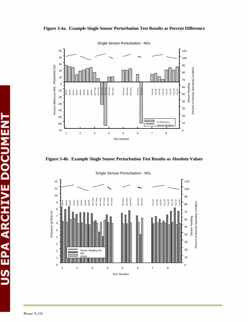
Figure 3-4a. Example Single Sensor Perturbation Test Results as Percent Difference

Single Sensor Perturbation - NOx

50

Igni

tion

Igni

tion

Igni

tion

Igni

tion

Igni

tion

Igni

tion

Igni

tion

Igni

tion

AM

Tem

p

AM

Tem

p

AM

Tem

p

AM

Tem

p

AM

Tem

p

AM

Tem

p

AM

Pre

ss

AM

Pre

ss

AM

Pre

ss

AM

Pre

ss

AM

Pre

ss

Fue

l DP

Fue

l DP

Fue

l DP

Fue

l DP

Fue

l DP

Fue

l DP

Fue

l DP

Fue

l DP

110

40 100

30 90

20 80

10 70

0

Per

cent

diff

eren

ce (

RM

- P

EM

S)/

RM

*100

Per

cent

of N

orm

al O

pera

ting

Con

ditio

n

Sen

sor

Rea

ding

60 -10

50 -20

-30

-40

-50

-60

-70

40

30

20

% Difference 10 Sensor Reading

0 7 81 2 3 4 5 6

Run Number

Figure 3-4b. Example Single Sensor Perturbation Test Results as Absolute Values

Single Sensor Perturbation - NOx

110

100

90

Igni

tion

Igni

tion

Igni

tion

Igni

tion

Igni

tion

Igni

tion

Igni

tion

Igni

tion

AM

Tem

p

AM

Tem

p

AM

Tem

p

AM

Tem

p

AM

Tem

p

AM

Tem

p

AM

Pre

ss

AM

Pre

ss

AM

Pre

ss

AM

Pre

ss

AM

Pre

ss

Fue

l DP

Fue

l DP

Fue

l DP

Fue

l DP

Fue

l DP

Fue

l DP

Fue

l DP

Fue

l DP

Sensor Reading (%) RM PEMS

12

11

10 S

enso

r R

eadi

ng

Per

cent

of N

orm

al O

pera

ting

Con

ditio

n9

8

7

6

5

4

3

80

70

60

50

40

30

Em

issi

ons

(g/ B

Hp

-hr)

20

10

2

1

0 0 1 2 3 4 5 6 7 8

Run Number

Page 3-10

�

��

=

4.0 FIELD TESTING AND CALCULATION PROCEDURES

4.1. OVERVIEW

The procedures described in this section provide a framework for testing a PEMS during both normal and off­normal engine operation. They are based on EPA Performance Specification Test guidelines for CEMS (40 CFR 60, Appendix B), EPA Reference Methods for determination of emission rates (40 CFR 60, Appendix A), and the document “Example Specifications and Test Procedures for Predictive Emission Monitoring Systems” provided by EPA’s Emission Measurement Center (Emission Measurement Center, 1999).

4.1.1. Determination of Relative Accuracy

For each of the gases for which concentrations and/or emission rates are predicted by a PEMS, the parameter that should be used to represent the result of the PEMS/Reference Method comparison is Relative Accuracy. Relative Accuracy should be calculated in accordance with the four-step process outlined below.

First, calculate the arithmetic mean of the difference, d, for all runs conducted as in Equation 1 below:

n1=d d in (Eqn. 1) i =1

][

Where: n = number of runs di = difference between Reference Method and PEMS output for a run

Second, calculate the standard deviation associated with all runs, Sd, as shown in Equation 2 below:

n 2

d i i 1

1 Ø ø 2 Œ ŒŒ ŒŒ ŒŒ ŒŒŒº

œ œœ

n

d 2 -i œœS d = 1 n (Eqn. 2) i =

n - 1 œœœœœß

Third, calculate the 2.5 percent error confidence coefficient (one-tailed), cc, as shown in Equation 3 below:

S dcc = t0 . 975 (Eqn. 3) n

Where: t0.975 = t-value (see Table 4-1).

Page 4-1

Table 4-1. t-Values

n* t0.975 n* t0.975 n* T0.975

2 12.706 7 2.447 12 2.201

3 4.303 8 2.365 13 2.179

4 3.182 9 2.306 14 2.160

5 2.776 10 2.262 15 2.145

6 2.571 11 2.228 16 2.131

* The values in this table are already corrected for n-1 degrees of freedom. individual runs.

Use n equal to the number of

Fourth, calculate the Relative Accuracy, RA, for all runs as shown in Equation 4 below:

100RA = [d + cc ] RM (Eqn. 4)

Where:

d = Absolute value of the mean differences (from Eqn. 1)

cc = Absolute value of the confidence coefficient (from Eqn. 1)

RM = Average Reference Method value

The test procedures suggested for utilization in this guideline are Federal Reference Methods. Reference Methods are well documented in the Code of Federal Regulations, include detailed procedures, and generally address the elements listed below (40CFR60, Appendices A and B).

• Applicability and principle • Range and sensitivity • Definitions • Measurement system performance specifications • Apparatus and reagents • Measurement system performance test procedures • Emission test procedure • Quality control procedures • Emission calculations • Bibliography

Page 4-2

Each of the selected testing methods utilizing an instrument measurement technique includes performance-based specifications for the gas analyzer used. These performance specifications cover span, calibration error, sampling system bias, zero drift, response time, interference response, and calibration drift requirements. An overview of each test method suggested for use is presented in this section, with emphasis on the type of monitors to be used, the monitor range, the sampling system configuration, and general calibration plans. The entire method reference will not be repeated here, but should be available to site personnel during testing, and can be viewed in Appendix A of 40CFR60 (www.epa.gov/cfr40.htm). Field log forms that can be used to conduct calibrations and other field activities are presented in Appendix A. Sample Reference Method output formats and summaries are also presented in Appendix A.

4.2. S A M P L E H A N D L I N G A N D T E S T I N G M E T H O D S

4.2.1. Sample Conditioning and Handling

A schematic of the sampling system used for the ANR test is presented as Figure 4-1. In order for some of the instruments used to operate properly and reliably, the flue gas must be conditioned prior to introduction into the analyzer if conditions are outside acceptable instrument parameters. The gas conditioning system shown in this figure is designed to remove water vapor and/or particulate from the sample. All interior surfaces of the gas conditioning system are made of stainless steel, Teflon™, or glass to avoid or minimize any reactions with the sample gas components. Gas is extracted from the gas stream through a heated stainless steel probe, filter, and sample line and transported to two ice bath condensers on each side of the sample pump. The condensers remove moisture from the gas stream. The clean, dry sample is then transported to a flow distribution manifold where sample flow to each analyzer is controlled. Calibration gases can be routed through this manifold to the sample probe by way of a Teflon™ line. This allows calibration and bias checks to include all components of the sampling system. The distribution manifold also routes calibration gases directly to the analyzer when linearity checks are made on each of the analyzers (other than the THC analyzer).

Page 4-3

Figure 4-1. Gas Sampling and Analysis System

F I L T E R

Condenser THC analyzer

O 2/CO2

analyzer CO

analyzer NOx

analyzer

Data acquisition

system

Post-pump condenser

Sample line and calibration gases

Cal gas

vent

Probe

( sample in) Heated sample lines

Sample gas manifold

Condensate pumps

O2

analyzer

The time required for sample gas to travel from the probe tip to the analyzers and obtain a stable response (i.e., the system response time) must be determined to ensure that time-matched comparisons of PEMS and Reference Method outputs are made. The sampling system response time should be measured at the beginning of field testing. The procedure should include the following stepwise process for each analyzer used:

1. Initiate a flow of zero concentration calibration gas at the probe and wait for stable readings to occur,

2. Introduce a high concentration calibration gas at the probe while simultaneously recording the start time,

3. Record the time at which the gas concentrations due to the step increase are at 95 percent of their expected level, and

4. Repeat the procedure going from high range gas to zero gas, record that time, and record the system response time for that pollutant as the longer of the two.

The final system response time is the longest response time recorded for an individual test parameter over the whole range of analyzers in use.

In addition to the system response time test, a flue gas stratification test should be conducted prior to the start of testing to determine the most representative location to position the reference method sampling probe. The

Page 4-4

procedures specified in Reference Method 20 for determination of NOX emissions from gas turbines should be followed. Since most engine exhaust ducts are less than 16 square feet in diameter, 8 traverse points are sufficient to check for stratification. Using a calibrated sampling system, measure the O2 or CO2 concentration in the exhaust gas stream at each of the 8 traverse points selected. If the concentrations are consistent at each of the 8 points, position the probe tip near the GHG Center of the duct for sampling. If the concentrations vary by 5 percent or more at one or more of the points, position the probe at the point where the value nearest to the average O2 or CO2 concentration was measured.

4.2.2. Calibrations

Calibrations should be conducted on all monitors using Protocol No. 1 calibration gases. Protocol No. 1 gases comply with requirements for traceability to the National Institute of Standards and Technology.

Each monitor should be calibrated with a zero concentration gas. In addition, each should be calibrated with a suite of gases, selected to cover the monitor operating ranges specified later in Section 4. The NOX, CO2, and O2

monitors should be calibrated with two additional gas concentrations each. One concentration should be 40 to 60 percent of span and one should be 80 to 100 percent of span. Maximum and actual pollutant concentrations anticipated for the test engine should be determined prior to the test to aid in selecting appropriate calibration gases and setting instrument ranges. The CO and THC monitors should be calibrated with three additional gas concentrations. For CO, the concentrations should include one each at approximately 30 , 60 , and 90 percent of span. For THCs, methane should be used if this is consistent with the basis that PEMS uses to report THCs (i.e., THC concentrations quantified as methane). The calibration concentration ranges for THCs includes the following: 25 to 35 percent, 45 to 55 percent, and 80 to 90 percent of span.

All monitor calibrations should be conducted daily, before sampling begins. Calibrations should start by routing calibration gases directly to each monitor using the sample gas manifold, and then adjusting the monitors to read the appropriate calibration gas values. Note that the THC monitor calibrations are conducted through the entire system only, not directly to the analyzer. After adjustments are made to the analyzers, a final linearity test should be conducted by introducing each gas to the analyzers and recording responses while making no adjustments. In accordance with Reference Method Criteria, an analyzer response within two percent of the span (range) of the analyzer is acceptable. Following this and after each test run, zero concentration and mid­span gases should be passed through the entire sampling system, and the values that are measured should be recorded. Differences between the initial calibration and these system calibrations should be used to determine system bias and drift values for each run and analyzer drift over the duration of each run. After field operations are complete, these bias and drift values should be used to adjust measured Reference Method concentrations before comparing the values to PEMS predictions. Details regarding the equations used to calculate these corrections are provided in the corresponding Reference Method.

Regarding engine sensor calibrations, the testing entity should obtain copies of the most recent calibration records for all of these sensors. If PEMS predictions do not agree well with Reference Method values during the testing, these records may help in determining if the problem is related to sensor accuracy, or PEMS algorithm problems.

4.2.3. Reference Method 3A – Determination of Oxygen & Carbon Dioxide Concentrations

For CO2 and O2, a continuous sample should be extracted from the emission source and passed through instrumental analyzers. For determination of CO2 a non-dispersive infrared (NDIR) analyzer or equivalent should be used. This type of instrument measures the amount infrared light that passes through the sample gas versus a reference cell. As CO2 absorbs light in the infrared region, the light attenuation is proportional to the CO2 concentration in the sample. The CO2 monitor range should be set at 0 to 20 percent CO2.

Page 4-5

Oxygen should be analyzed using a fuel cell, electrochemical cell, or paramagnetic analyzer or equivalent. The fuel cell and electrochemical cell analyzers use electrolytic concentration cells that contain a solid electrolyte to enhance electron flow to the O2 as it permeates through the cell. The technology used by this type of instrument determines levels of O2 based on partial pressures. The electrode is porous (zirconium oxide) and serves as an electrolyte and as a catalyst. The sample side of the reaction has a lower partial pressure than the partial pressure in the reference side. The current produced by the flow of electrons is directly proportional to the O2

concentration in the sample. The paramagnetic technology used by this instrument determines levels of O2

based on the level of physical deflection of a diamagnetic material caused by exposure to the stack gas. The higher the O2 concentrations, the greater the material is deflected. An optical system with an amplifier detects the level of deflection, which is linearly proportional to the O2 level in the gas. The O2 monitor range should be set at 0 to 25 percent O2.

4.2.4. Reference Method 7E - Determination of Nitrogen Oxides Concentration

Nitrogen oxides should be determined on a continuous basis, utilizing a chemiluminescence analyzer. This type of analyzer catalytically reduces nitrogen oxides in the sample gas to NO. The gas is then converted to excited NO2 molecules by oxidation with O3 (normally generated by ultraviolet light irradiation of air or oxygen). The resulting NO2 luminesces in the infrared region. This emitted light is measured by an infrared detector and reported as NOX. The intensity of the emitted energy from the excited NO2 is proportional to the concentration of NO2 in the sample. The efficiency of the catalytic converter in making the changes in chemical state for the various nitrogen oxides is checked as an element of instrument set up and checkout. The appropriate NOX

monitor range should be set based on preliminary site-specific data collected before starting the test. More than one range may be needed if measured NOX concentrations vary widely between different engine load and speed operations. In any case, measured NOX concentrations should be greater than 30 percent of the analytical range selected, and no readings should be higher than the selected range.

4.2.5. Reference Method 10 - Determination of Carbon Monoxide Concentration

For Reference Method 10, a gas filter correlation analyzer utilizing an optical filter arrangement and NDIR detection or equivalent should be used. The method chosen should provide high specificity for CO.

In the instrument suggested gas filter correlation utilizes a constantly rotating filter with two separate 180­degree sections (much like a pinwheel.) One section of the filter contains a known concentration of CO, and the other section contains an inert gas without CO. The sample gas is passed through the sample chamber containing a light beam in the region absorbed by CO. The sample is then measured for CO absorption with and without the CO filter in the light path. Based upon the known concentrations of CO in the filter, these two values are correlated to determine the concentration of CO in the sample gas. An appropriate CO analyzer operating range should be selected as described in Section 4.2.4.

4.2.6. Reference Method 25A - Determination of Total Gaseous Organic Concentration

Total hydrocarbon vapors in the exhaust gas should be measured using a flame ionization (FID) analyzer. The method used by the FID passes the sample through a hydrogen flame. The intensity of the resulting ionization is amplified, measured, and then converted to a signal proportional to the concentration of hydrocarbons in the sample. Unlike the other reference methods, the sample stream going to the FID analyzer does not pass through the condenser system, so it can be kept heated until it is analyzed. This is necessary to avoid loss of the less volatile hydrocarbons in the gas sample. Because all combustible hydrocarbons are being analyzed and reported, the emission value must be calculated to some base (methane or propane). The calibration gas for THCs should be either methane or propane; which ever is consistent with the basis on which the PEMS reports THC values. An appropriate THC analyzer operating range should be selected as described in Section 4.2.4.

Page 4-6

4.2.7. Determination of Emission Rates

If the PEMS predicts emissions in units of mass per unit time, use Reference Method 19 to convert measured concentration values of the exhaust gases to emission rate values. This is accomplished by determining the volumetric flow rate of the exhaust gas and then calculating the emission rate from the concentration and volume data. The fundamental principle of this method is based upon F-factors, which are the ratio of combustion gas volume to the heat content of the fuel. F-factors are calculated as a volume/heat input value, (e.g., standard cubic feet per million Btu). This method applies only to combustion sources for which the heating value for the fuel can be determined. The F-factor can be calculated from measured CO2 or O2

concentrations. This method includes all calculations required to compute the F-factors and guidelines on their use. The F-factor for natural gas should be calculated from gas compositional measurements (elemental analyses and lower heat content). Many facilities can provide these analyses using pipeline gas chromatograph (GC) data. If not, gas samples can be collected and submitted to a laboratory for analysis, or the F-factors published in Reference Method 19 can be used.

Other parameters needed to complete the Method 19 conversions to mass rate include fuel flow rate measured by a fuel flow monitoring system (pressure and temperature based), and calculated engine brake horsepower (can be calculated from engine speed and torque readings per operator based methods). The step-by-step calculations involved are listed below.

Step 1. Normalize measure pollutant concentrations to heat input.

Concentration (lb/MBtu) = measured concentration (lb/scf) x F-factor (scf/MBtu)

Step 2. Calculate the engine heat consumption rate in million Btu per hour.

Heat consumption (MBtu/hr) = measured fuel flow (scfh) x fuel heating value (MBtu/ft3)

Step 3. Calculate emission rate as pounds per hour of pollutant.

Emission rate (lb/hr) = concentration (lb/Mbtu) x engine heat consumption (Mbtu/hr)

Step 4. Normalize emission rates to engine output as grams per brake horsepower hour (g/BHp-hr).

Emission rate (g/BHp-hr = (emission rate (lb/hr) x 453.59 gms/lb) / engine output (BHp-hr)

As an alternative to Method 19 for determination of emission rates, exhaust gas volumetric flow rate can be determined using actual stack gas measurements. This testing is done in accordance with EPA Reference Methods 1 through 4 and involves determining exhaust gas velocity and molecular weight, and using these measurements along with the measured stack cross-sectional area to calculate gas volumetric flow rate. This procedure is fully documented in the Reference Methods and not repeated here. However, this procedure can only be conducted on engine exhaust stacks that have sufficient straight run of pipe, acceptable test ports with safe access, and laminar flow characteristics.

4.3. DATA ACQUISITION

Output from each of the instruments should be transmitted to a data acquisition system, typically a personal computer-based data acquisition system. The system clock should be synchronized with the PEMS and the engine control systems. This system should be configured to receive signals from all of the instruments every

Page 4-7

two seconds, and integrate those values over a pre-specified averaging period. During all tests, a 30-second averaging period should be used for each monitored parameter, and these values should be stored for later analysis and reporting purposes. Average values should also be determined over the time associated with each run, and these values should be stored and used to determine run-average emissions for Relative Accuracy and other determinations. Computer spreadsheets (ExcelTM or other) can be used to calculate calibration results, and make corrections to the data for calibration, system bias, and drift values.

Data should also be collected on engine performance parameters, and these data should be provided by either the operator or PEMS data acquisition systems. These data will be needed to calculate some verification parameters, identify alarm/alert conditions, and interpret verification results. Data should be recorded at 30­second intervals, and then averaged for each test period.

Page 4-8

5.0 DATA VALIDATION, QUALITY ASSESSMENT, AND REPORTING

5.1. DATA VALIDATION

Quality control checks for the Reference Method measurements were presented in Section 4.2.2. Upon review, all data collected should be classified as valid, suspect, or invalid. In general, valid results are based on measurements that meet data quality goals, and that were collected when an instrument was verified as being properly calibrated.

Often anomalous data are identified in the process of data review. All outlying or unusual values should be investigated daily in the field using test records, test crew and engine operator interviews, and log forms. Anomalous data may be considered suspect if no specific operational cause to invalidate the data is found. All data, whether valid, invalid, or suspect, should be included in the final report. However, report conclusions should be based on valid data only. The reasons for excluding any data should be justified in the report. Suspect data may be included in the analyses, but may be given special treatment as specifically indicated.

All engine sensor and Reference Method data should be reviewed in the field by a designated field team leader on a daily basis including those listed below.

• Run average comparison of Reference Method and PEMS data for agreement based on arithmetic mean, standard deviation, and Relative Accuracy for each measured parameter

• Daily Reference Method calibration results and run-specific zero and mid-span calibration results

5.2. DATA QUALITY

As a consequence of using EPA Reference Methods to verify PEMS performance, measurement methodologies and data quality determinations are defined. Reference Method procedures ensure that run-specific quantification of instrument and sampling system drift and bias occurs, and that runs are repeated if specific performance goals are not met. Furthermore, the Reference Methods require adjustments be made to all measured concentrations based on run-specific measurements of instrument and sampling system responses to calibration checks. Normally, measurements of these data quality indicators would be used to quantify the data quality achieved during testing, but in this case, these data are used to adjust measured values to ensure that the highest possible representativeness and quality exists in the final results. Therefore, the Relative Accuracy and other determinations conducted are considered to be of acceptable quality if all Reference Method calibrations, performance checks, and concentration corrections specified in the Reference Methods have been successfully conducted. As such, the Data Quality Objective (DQO) for all runs is to ensure that this has occurred. Evidence of the successful execution of these requirements should be documented in the verification report, along with run- and pollutant-specific calibration results.

Specific data quality indicators are discussed below including indicators for completeness, precision, and bias. These apply to all of the verification parameters that should be assessed. A summary of the data quality indicator goals is shown in Table 5-1.

1. Completeness should be 100 percent for the Relative Accuracy determinations. This means that data must meet the DQOs (analyzer and system calibration criteria) for all RATA runs conducted. Runs that don’t meet the

Page 5-1

DQO should be repeated. The completeness goal for the off-normal engine operating tests should be 85 percent. This goal is lower than 100 percent to account for potential difficulties that may occur in (1) establishing abnormal engine operating conditions planned for this series of tests, and (2) measuring potentially large and dynamic pollutant concentration profiles in a manner that meets the DQO. Finally, the completeness goal for the sensor drift tests is 100 percent, which means that all runs should be conducted, as outlined in 3.3.2, that meet the DQO above, or be repeated. During the verification of the ANR PEMS, all of these completeness goals were met.

2. System accuracy or bias assessments should be conducted at the beginning of each day using the protocols defined in each Reference Method. This should be accomplished by routing a suite of calibration gases directly into each monitor. For each calibration gas concentration examined, a data quality indicator goal of – 2 percent of the analyzer span value should be used for O2, CO2, NOX, and CO. A goal of – 5 percent of the calibration gas value should be used for THCs. Daily accuracy values determined from these evaluations should be reported in the final verification report to document the ability of the testing entity to achieve the accuracy indicator goals specified above. These accuracies should be determined in the field, and if deviations from the goals are observed, sampling should be halted by the testing entity until corrective action is taken. A corrective action is the process that occurs when the result of an audit or quality control measurement is shown to be unsatisfactory, as defined by the data quality objectives or by the measurement objectives for each task. The corrective action process involves the Field Team Leader, Project Manager, and QA Manager. In cases involving the analytical process, the correction action will also involve the analyst. A written Corrective Action Report is required on all corrective actions (Example in Appendix A).

3. System precision or bias should be determined for the combined sampling system and analyzer at the beginning and end of each run using the protocols defined in each Reference Method. This is accomplished by routing zero concentration and mid-span gases through the sample collection lines and monitor systems, and comparing the measured concentrations with the certified calibration values. System bias, determined in this manner, should be measured before and after each run to determine if the run is acceptable for use. A drift of greater than – 3 percent of analyzer span (difference between the before and after system bias) should be considered unacceptable, and the run should be repeated. If a drift of less than 3 percent occurs, which is the data quality indicator goal for precision, the average of the before and after system bias values should be used to correct the measured concentrations in each of the Reference Methods. All system bias values and calculated drift values should be reported in the final verification report on a run-specific and gas specific basis as a means of documenting that this data quality indicator goal has been achieved.

Table 5-1. Data Quality Indicator Goals

Data Quality Indicator

Type of Verification Test Relative Accuracy Off-Normal Engine Sensor-Failure

Completeness 100 % 85 % 100 % Precision Drift < – 3% of span Drift < – 3% of span Drift < – 3% of span

Accuracy – 2 % of spana

– 5 % of cal. conc.b – 2 % of spana

– 5 % of cal. conc.b – 2 % of spana

– 5 % of cal. conc.b

a O2, CO2, NOX, and CO b THCs

In addition to these quality control measures, independent systematic checks to determine the quality of the data should be performed on the activities of this type of evaluation. Under the ETV Program, these checks consist

Page 5-2

of a performance evaluation audit and data audit as described below. In addition, the internal quality control measurements are used to assess the performance of the analytical methodology. The combination of these audits and the evaluation of the internal quality control data allow the assessment of the overall quality of the data for the evaluation.

Under the ETV program, a designated QA Manager is responsible for ensuring the audits are conducted as required by the site specific Test/QA Plan. Audit reports that describe problems and deviations from the procedures are prepared and distributed to the Field Team Leader. Any problems or deviations need to be corrected. The Field Team Leader is responsible for evaluating corrective action reports, taking appropriate and timely corrective actions, and informing the QA Manager of the action taken. The QA Manager is then responsible for ensuring that the corrective action was taken. A summary report of the findings and corrective actions is prepared and distributed to the Project Manager and Center Director.

Performance Evaluation Audit

The performance evaluation audit (PEA) is designed to check the operation of the emissions testing analytical system. The method of performance will be based on internal audits performed by the Field Team Leader. For an evaluation of this type, a blind audit of one or more of the analyzers can represent the PEA. Calibration gases can be obtained with known (certified) concentrations of NOX, CO, and/or THCs and be presented to the Entech analyst in such a manner as to have the concentration of the PEA unknown (blind) to the analyst. Upon receiving the analytical data from the analyst, the Field Team Leader will evaluate the performance data for compliance with the requirements of the project. The PEA must occur on-site during the field test.

Audit of Data Quality

The audit of data quality (ADQ) is an evaluation of the measurement, processing, and evaluation steps to determine if systematic errors have been introduced. During the ADQ, the QA Manager, or designee, will randomly select approximately 10 percent of the data to be followed through the analysis and processing the data. The scope of the ADQ is to verify that the data-handling system is correct and to assess the quality of the data generated.

The ADQ, as part of the system audit, is not an evaluation of the reliability of the data presentation. The review of the data presentation is the responsibility of the Project Manager and the technical peer reviewer.

5.3. REPORTING

At the completion of the evaluation, a draft verification report and Statement is prepared by the Project Manager. Under the ETV Program, the final verification report contains a verification statement, which is a 3 to 4 page summary of the PEMS tested, the test strategy used, and the verification results obtained. The verification report summarizes the results for each verification parameter discussed in this guideline and contains sufficient raw data to support findings and allow others to assess data trends, completeness, and quality. Clear statements should be provided which characterize the performance of the verification parameters. An example outline of the report is shown below.

Example Verification Report Outline

Verification Statement

Page 5-3

Section 1: Verification Test Design and Description Identification of Participants PEMS system and site description Overview of the verification parameters and evaluation strategies

Section 2: Results Relative Accuracy Determinations PEMS Prediction Capabilities During Abnormal Engine Operation PEMS Response to Sensor Failure

Section 3: Data Quality Assessment

Section 4: Additional Technical and Performance Data (optional)

Appendices: Raw Verification and Other Data

Page 5-4

6.0 BIBLIOGRAPHY

Buchop, Thomas Robert, et al. “Parametric Emissions Monitoring System Having Operating Condition

Deviation Feedback.” United States Patent Number 5,703,777. United States Patent Office. Washington, DC.

December 30, 1997.

Code of Federal Regulations, Title 40, Part 60 (Appendices A and B). United States Environmental Protection

Agency. Washington, DC. 1999.

Code of Federal Regulations, Title 40, Parts 64 (Appendix C) and 75 (Appendix E). United States

Environmental Protection Agency. Washington, DC. 1999.

“Example Specifications and Test Procedures for Predictive Emission Monitoring Systems.” Emission

Measurement Center. United States Environmental Protection Agency. Research Triangle Park, NC. 1999.

Document can be obtained from the following Internet location www.epa.gov/ttn/emc/cem.html.

Page 6-1

APPENDIX A

SampleField Data Log Forms

andData Acquisition System Outputs

Page A-1

SAMPLEFIELD DATALOG FORMS

Page A-2

PEMS INSTALLATION/SET-UP CHECKLIST

Completed by:__________________________________ Date:__________

Complete Y/N/na

ACTIVITY/ITEM REMARKS (if needed, continue on reverse side by item)

Software installation and checkout completed

Verify critical sensors – number, model

Sensor input present on engine computer, correct range

Procure sensor calibration data

Verify PEMS printouts available and include identification of

engine, date, time, all emission values, and alarms

Verify and document engine I.D.

NOTES:

Page A-3

TESTING SET-UP/PREPARATION CHECKLIST

Completed by:__________________________________ Date:__________

Complete Y/N/na

ACTIVITY/ITEM REMARKS (if needed, continue on reverse side by item)

Identify test team participants and team leader

Identify contact person for PEMS and engine operation

Identify test team Reference Method system – model, serial number, wet or dry basis

Identify operating range and calibration gases – contents, concentrations, cylinder s/n calibration certificate

Verify interference tests documented or completed

Verify and document results of NO2 to NO conversion test

Verify DAS printout is complete

Verify stratification testing and document results

Verify integrity of the sampling system, multi-point sampling, and document location of calibration gas injection Document system leak check

NOTES:

Page A-4

TESTING SET-UP/PREPARATION CHECKLIST (continued)

Complete Y/N/na

ACTIVITY/ITEM REMARKS (if needed, continue on reverse side by item)

Document system response times

Synchronize PEMS and Reference Method Clocks Manually check DAS calculations

Document any data points requiring manual data collection and transfer list to “Test Run Observation Checklist”

NOTES:

Page A-5

TEST RUN OBSERVATION CHECKLIST (Note: Complete a checklist for each test run)

Completed by:__________________________________ Date:__________

Complete Y/N/na

ACTIVITY/ITEM REMARKS (if needed, continue on reverse side by item)

Document planned test conditions (from test matrix)

Pre-test calibrations on sampling systems completed? Documented?

Atmospheric conditions Temperature__________ Barometric Press._________ RH _________ Wind speed/direction________/________

Start time for test run Test Start__________

Document actual test conditions

Verify PEMS and Reference Method System are collecting required data points

Verify all manually collected data are documented

End time for test run Test end__________

Post-test calibration of sampling systems completed

Bias determined and applied to data

NOTES:

Page A-6

TEST RUN OBSERVATION CHECKLIST (continued)

Complete Y/N/na

ACTIVITY/ITEM REMARKS (if needed, continue on reverse side by item)

Copy of Reference Method test run data obtained Verify completeness

Copy of PEMS test run data obtained Verify completeness

Document all anomalies and unexpected events/conditions

DAS output obtained?

Obtain gas composition data?

NOTES:

Page A-7

______________________________________________________

______________________________________________________

______________________________________________________

_____________________________________________________

_____________________________________________________

_____________________________________________________

______________________________________________________

______________________________________________________

______________________________________________________

Corrective Action Report

Verification Title: ________________________________ Verification Description: __________________________

Description of Problem: _________________________________

Originator: _______ Date: ________

Investigation and Results: ______________________________

Investigator: _______ Date: ________

Corrective Action Taken: _______________________________

Originator: _______ Date: ________ Approver: _______ Date: ________

Carbon copy: Project Manager, Center Director, Center QA Manager, Pilot Manager

Page A-8

SAMPLEREFERENCE METHOD

DATA ACQUISITION SYSTEMOUTPUTS

Page A-9

PLANT NAME: UNIT # :

LOCATION: DATE:

REFERENCE METHOD CONTINUOUS MONITORING DIFFERENCE

START END lb NOx / lb NOx / lb NOx / RUN # TIME TIME ppmd NOx %w CO2 mmBtu ppmd NOx %w CO2 mmBtu ppmd NOx %w CO2 mmBtu

1 0:00 0:30 268.80 13.28 0.435 265.05 13.08 0.436 3.75 0.20 -0.001

2 12:01 12:31 274.23 13.34 0.442 264.45 13.05 0.436 9.78 0.29 0.006

3 12:47 13:17 279.63 13.21 0.455 261.90 13.03 0.432 17.73 0.18 0.023

4 13:30 14:00 275.21 13.35 0.443 264.50 13.03 0.436 10.71 0.32 0.007

5 14:15 14:45 272.02 13.27 0.441 262.85 12.97 0.436 9.17 0.30 0.005

6 15:00 15:30 272.58 13.27 0.441 259.75 13.03 0.428 12.83 0.24 0.013

7 15:45 16:15 268.34 13.25 0.435 253.40 12.94 0.421 14.94 0.31 0.014

8 16:30 17:00 271.52 13.28 0.439 254.50 12.94 0.423 17.02 0.34 0.016

9 17:30 18:00 268.61 13.28 0.435 252.75 12.99 0.418 15.86 0.29 0.017

* 10

* 11

* 12

Test Mean: 272.33 13.28 0.441 259.91 13.01 0.430

MEAN DIFFERENCE: 12.42 0.27 0.01

NOx Conversion Factor: 1.194E-07 lb NOx / SCF - ppm NOx Fc - Factor: 1800 SCF / mmBtu STANDARD DEVIATION: 4.52 0.06 0.01

CONFIDENCE COEFFICIENT: 3.47 0.04 0.01 _

Bias Adjustment Factor = (1 + d / CEM ) RELATIVE ACCURACY (%): 5.84 2.39 3.81 _

WHERE: d = Mean of the Differences BIAS ADJUSTMENT FACTOR: 1.026

CEM = Mean of the Source Monitor's Data Values T - VALUE: 2.306

* Run not included in Relative Accuracy Calculations

Page A-10

Reference Method Values Corrected for Bias & Drift

PLANT NAME: UNIT #: RUN #:

START TIME:END TIME: DATE:

CAL GAS VALUE INITIAL CAL FINAL CAL AVERAGE CAL

0 . 0 0 ppm SO2 4 . 1 5 2 . 6 9 3 . 4 2 443 .00 ppm SO2 435 .41 439 .80 437 .61

0 . 0 0 ppm NOx 1 . 2 2 0 . 7 3 0 . 9 8 463 .60 ppm NOx 437 .36 439 .80 438 .58

0 . 0 0 % O2 0 . 1 8 0 . 4 3 0 . 3 1 1 2 . 1 2 % O2 1 2 . 1 5 1 2 . 2 7 1 2 . 2 1

0 . 0 0 % CO2 0 . 1 5 -0 .05 0 . 0 5 1 1 . 5 0 % CO2 1 1 . 3 8 1 1 . 4 8 1 1 . 4 3

Raw Data: 223 .11 ppm SO2 257 .27 ppm NOx

6 . 4 1 % O 2 1 3 . 1 9 % CO2 0 . 0 0 0 % H2O

CORRECTED VALUES: 224 .15 ppmw SO2 271 .52 ppmw NOx

1 3 . 2 8 %w CO2 0 . 4 3 9 lb NOx / mmBtu

6 . 2 2 %d O2 1 3 . 2 8 %d CO2

CONVERSION FACTORS: N O x = 1 .194E-07 lb NOx / SCF - ppm NOx

Fc - FACTOR = 1 8 0 0 SCF / mmBtu

SAMPLE CALCULATIONS: _

CORRECTED VALUES = Cma * (C - Co) / (Cm - Co) _

WHERE: C = MEAN REFERENCE MEASUREMENT

C o = MEAN ZERO CALIBRATION RESPONSE Cm = MEAN MID OR UPSCALE CALIBRATION RESPONSE

Cma = ACTUAL MID OR UPSCALE CAL GAS CONCENTRATION

EMISSION RATE = (ppm)(Conversion Factor)(Fc-Factor)(100 / % CO2)

Page A-11

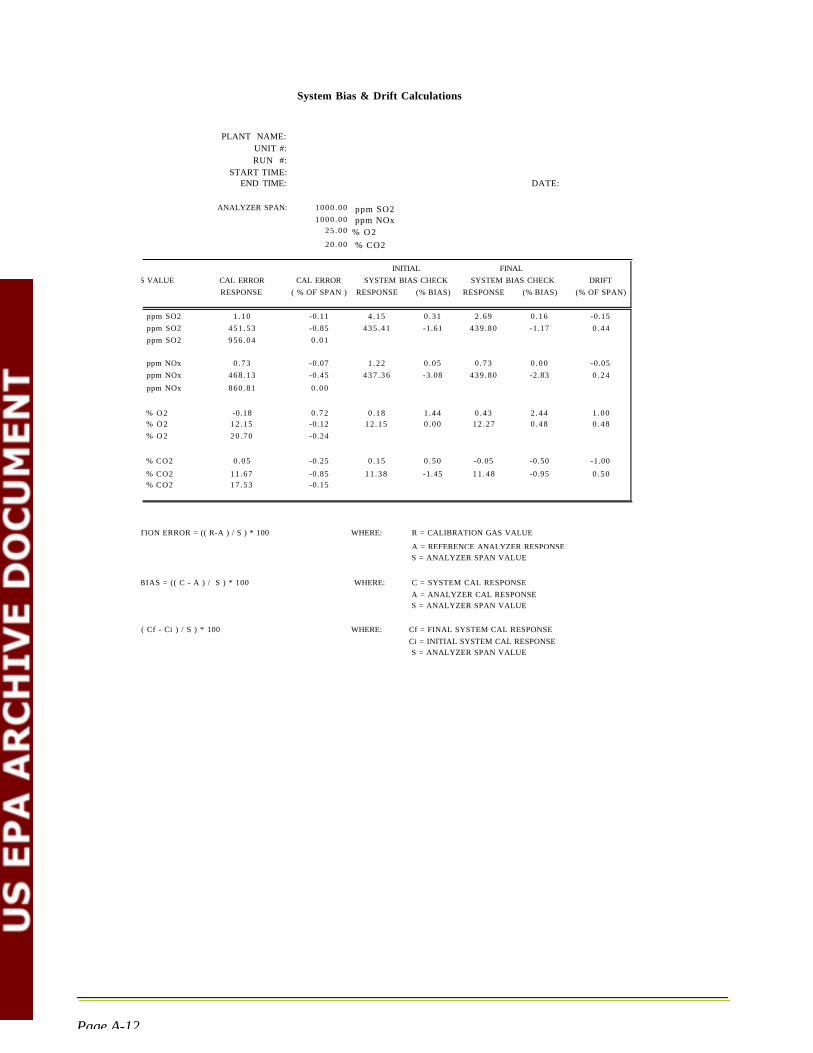
UNIT #: RUN #:

System Bias & Drift Calculations

PLANT NAME: UNIT #: RUN #:

START TIME: END TIME: DATE:

ANALYZER SPAN: 1000 .00 ppm SO2 1000 .00 ppm NOx

25 .00 % O 2 20 .00 % CO2

CAL GAS VALUE CAL ERROR

RESPONSE

CAL ERROR

( % OF SPAN )

INITIAL

SYSTEM BIAS CHECK

RESPONSE (% BIAS)

FINAL

SYSTEM BIAS CHECK

RESPONSE (% BIAS)

DRIFT

(% OF SPAN)

ppm SO2

ppm SO2

ppm SO2

1 .10

451 .53

956 .04

-0.11

-0.85

0 .01

4 .15

435 .41

0 .31

-1.61

2 .69

439 .80

0 .16

-1.17

-0.15

0 .44

ppm NOx

ppm NOx

ppm NOx

0 .73

468 .13

860 .81

-0.07

-0.45

0 .00

1 .22

437 .36

0 .05

-3.08

0 .73

439 .80

0 .00

-2.83

-0.05

0 .24

% O 2 % O 2

% O 2

-0.18 12 .15

20 .70

0 .72 -0.12

-0.24

0 .18 12 .15

1 .44 0 .00

0 .43 12 .27

2 .44 0 .48

1 .000 .48

% CO2

% CO2 % CO2

0 .05

11 .67 17 .53

-0.25

-0.85 -0.15

0 .15

11 .38

0 .50

-1.45

-0.05

11 .48

-0.50

-0.95

-1.00

0 .50

% CALIBRATION ERROR = (( R-A ) / S ) * 100 WHERE: R = CALIBRATION GAS VALUE

A = REFERENCE ANALYZER RESPONSE S = ANALYZER SPAN VALUE

% SYSTEM BIAS = (( C - A ) / S ) * 100 WHERE: C = SYSTEM CAL RESPONSE

A = ANALYZER CAL RESPONSE S = ANALYZER SPAN VALUE

% DRIFT = (( Cf - Ci ) / S ) * 100 WHERE: Cf = FINAL SYSTEM CAL RESPONSE

Ci = INITIAL SYSTEM CAL RESPONSE S = ANALYZER SPAN VALUE

Page A-12

Volumetric Flow Rate Determination

PLANT NAME: UNIT #: RUN #:

START TIME:END TIME:

DATE:TEST DATA

Test Delta P Temperature Stack Diameter (D): 367.00 inches

Point (in H2O) (Deg. F) Stack Area (A): 105,784 sq. inches A-1 0.530 126 Barometric Pressure (Pbar): 29.70 inches Hg

A-2 0.520 126 Static Pressure (Pg): -0.480 inches H2O

A-3 0.530 127 Percent O2 (% O2): 6.22 % O2 A-4 0.490 129 Percent CO2 (% CO2): 13.28 % CO2

A-5 0.530 128 Percent Nitrogen (% N2): 80.50 % N2

A-6 0.520 128 Pitot Tube Coefficient (Cp): 0.84 A-7 0.500 123 Meter Box Delta H (dH): 1.94 A-8 0.450 125 Meter Box Factor (Y): 0.9800 B-1 0.530 128 Average Meter Temp. (Tm): 67.300 degrees F

B-2 0.530 129 Gas Meter Volume (Vm): 23.838 cubic feet B-3 0.520 128 Impinger (V): 62 ml

B-4 0.470 125 Silica Gel (W): 3 .6 grams

B-5 0.540 125 B-6 0.520 125 B-7 0.510 125 Root Mean Sq. Delta P (Pavg): 0.5077 inches H2O

B-8 0.440 125 Mean Stack Temperature (Ts): 126.38 degrees F

MAX. MIN.

0.540 0.440

129 123

CALCULATIONS

Vm(std) = (Vm)(Y)(17.64((Pbar)/(Tm + 460))

Vwc(std) = (V)(.04707) + (W)(.04715) % H2O = [Vwc(std) / (Vwc(std) + Vm(std))] x 100

Mfd = 1 - (%H2O / 100) Ps = Pbar + (Pg / 13.6)

Md = 0.44(% CO2) + 0.32(% O2) + 0.28(% N2) Ms = (Md)(Mfd) + 0.18(% H2O)

Vs = 85.49 (Cp) x SQRT[(Pavg)(Ts + 460) / (Ps)(Ms)] Qsd = (60 / 144)(Mfd)(Vs)(A)(Ps / Pstd)(Tstd / (Ts + 460))

Qs = (3600 / 144)(Vs)(A)(Ps / Pstd)(Tstd / (Ts + 460)) Qaw = (60 / 144)(Vs)(A)

Vm(std) = 23.211 dscf

Vwc(std) = 3.0834 cubic ft. % H2O = 11.726 % H2O

Mfd = 0.883 P s = 29.665 in. Hg

Md = 30.374 lb/lb-mole M s = 28.931 lb/lb-mole

V s = 42.29 ft/sec Q s d = 1 .469E+06 DSCFM

Q s = 9 .985E+07 SCFH Q a w = 1 .864E+06 ACFM

1664.1 Kscfm

Page A-13