grid impedance estimation for islanding detection and ...eprints.nottingham.ac.uk/44087/1/grid...

1

Grid Impedance Estimation for Islanding Detection and Adaptive Control of Converters

Abdelhady Ghanem1,2*, Mohamed Rashed1, Mark Sumner1, Mohamed. A. Elsayes2 and

Ibrahim. I. I. Mansy2

1Department of Electrical and Electronics Engineering, University of Nottingham, Nottingham, UK. 2 Electrical Engineering Department, Mansoura University, Mansoura, Egypt. *[email protected]

Abstract: Power system (grid) impedance is time varying due to the changing structure of the power system

configuration and it can have a considerable influence on the control and stability of grid connected converters. This

paper presents an online grid impedance estimation method using the output switching current ripple of a SVPWM

based grid connected converter. The proposed impedance estimation method is derived from the discretised system

model using two consecutive samples within a single switching period. The estimated impedance is used for islanding

detection and online current controller parameter tuning. Theoretical analysis and MATLAB simulation results are

presented to verify the proposed method and its effectiveness is validated using experimental testing.

1. Introduction

An increasing number of power electronic converters are being used to connect renewable energy sources to

the grid. In recent years, real-time grid impedance estimation has been researched to improve controller stability and

protection (e.g. with islanding detection) in these types of converter [1-3]. Methods for grid impedance estimation are

generally classified as passive (non-invasive) and active (invasive) [4]. Passive methods use the non-characteristic

(harmonic) voltage and current measurements inherently present in the system to estimate impedance whilst active

methods deliberately create a disturbance in the grid and the impedance is estimated from the grid response: in general

good results can be achieved as the injection gives the measurements used for impedance estimation a high signal to

noise ratio (SNR). Passive methods are preferred as they do not create additional disturbances in the grid, however,

the SNR is much lower and the estimate tends to be poorer.

Passive methods for example based on the disturbance induced during the connection of a capacitor bank have

been presented in [5, 6]. In [5], the authors measured the unbalanced voltage and current variation induced by

connecting a capacitor bank to only one phase of a 12 kV substation power system. The voltage and current before

and after the capacitor bank switching as well as the capacitor current are digitally recorded to estimate the self and

mutual system impedance at the harmonic frequencies using the Fast Fourier Transform (FFT). The precision of the

results is limited not only by the frequency of the harmonics present but also by their amplitudes, which become very

low with respect to noise for higher frequencies. In [6], the voltage and current before and after the switching of a 12

kV, 750 kVAr capacitor are recorded to estimate the system impedance. Two frequency domain methods are presented.

The first method uses the FFT and is named the direct method: the frequency components of the voltage and current

are identified, then the voltage and current spectra are used to find the impedance transfer function. This method was

found to produce accurate results when the frequency component SNRs are large. The second method (the indirect

method) first obtains an estimate of the voltage and current samples and then auto and cross-correlation functions are

employed to reject the frequency components that are contaminated with noise. These functions are then used together

with the FFT to find the respective power spectra of the signals, and finally to find the impedance transfer function.

However, this second method suffers from false cross correlations between the voltage and current.

A passive grid impedance estimation method based on the inherent switching features (high frequency

harmonics) of the grid-connected power converter is presented in [7]. This method achieved fast and accurate

impedance estimation. However, the current at the switching frequency is very small, so more consideration for SNR

and the measurement of a low amplitude current harmonic superimposed on a large fundamental are required. A grid

inductance estimation method based on the excitation of the LCL-filter resonance is proposed in [8]. The technique

presented is based on the fact that the frequency peak due to the resonance is particularly sensitive to a change of grid

inductance. The limitations of this method include exciting the system resonance in a controlled way and the high

number of calculations can overload the processing platform. In [9], an Extended Kalman Filter (EKF) is used to

estimate the time variant grid impedance. It uses an observer based parameter identification based on the inherent

mailto:*[email protected]

2

disturbance at the point of common coupling (PCC). The main disadvantage of this method is the complicated tuning

processes for the covariance matrices. Another example of a passive method [10] is an analytical estimation model

created in the stationary reference frame to estimate the total inductance seen by a variable switching frequency

converter using two consecutive current samples. However, the estimated inductance is sensitive to system resistance.

A major drawback of passive techniques is that the grid variations might not be sufficiently large enough to

give an accurate estimation of the grid impedance due to the low SNR. Another issue is the time interval at which grid

variations occur. It might be the case that no variations appear for a long time, hence no information about grid

impedance is known during this time interval. For this reason, it is known that passive methods have a very large non‐detection zone.

Several active techniques have been reported in recent years. Ciobotaru et al. [4] presented an online impedance

estimation technique based on periodical variations of active and reactive power (PQ variations) of a grid connected

single phase power converter. This technique is based on the intentional change of both active and reactive power in

order to produce a grid disturbance and hence grid impedance can be estimated. The accuracy of this method depends

on the PQ variation values and the duration of the perturbation. In [11, 12] a current spike is deliberately injected at

the voltage zero crossing instant by a grid connected converter. In order to eliminate the background grid disturbance

and harmonics, the voltage and current signals before the injection are measured and subtracted from their signals

during the injection. Based on the extracted voltage and current signals, the grid impedance value is determined using

a FFT. A similar method employing the Continuous Wavelet Transform (CWT) to derive the impedance from transient

data is presented in [13]. The main drawbacks of current spike injection based impedance estimation techniques are

that the system ratings may be exceeded and nonlinear system response may be excited. Asiminoaei et al. [14] have

used a PV inverter to inject a low frequency non-characteristic harmonic current of 75 Hz by adding a harmonic

voltage to the voltage reference of the PV inverter. A Discrete Fourier Transform (DFT) amplitude and phase

calculations are then performed to calculate the grid impedance at that frequency. In [15] an injection of a high

frequency signal comprising one or two voltage harmonic signals is implemented. The single harmonic injection uses

a 500 Hz signal and the double harmonic injection uses a 500 Hz and 600 Hz signals. The authors in [16], presented

a power network parameter estimation based on stimulations injected through a pulse width modulator: it creates a

stimulation signal based on Pseudo Random Binary Sequences (PRBS) which have been used to create harmonic-rich

stimulation.

Good impedance estimation can be achieved using the aforementioned active methods; however, they suffer

from various problems, mainly related to the rate and amplitude of the repeated injections which are usually kept high

to increase the SNR and adversely increase the total harmonic distortion. In addition, the estimated impedance

accuracy depends on the level of the background harmonics. Furthermore, complicated post-processing is always

required which may overload the processing platforms.

In this paper, an improved approach to passive impedance estimation is proposed. It uses closed form models

for grid inductance and resistance estimation derived from the discretised system model in a rotating reference frame.

It uses two consecutive samples within a single switching period of a SVPWM based converter – it could be argued

that it is using the PWM itself as an injection signal to obtain the benefit of improved SNR compared to most passive

methods. The proposed impedance estimation technique is capable of identifying the total inductance seen by the

converter. However, it is unable to identify the resistance of the grid impedance. The proposed impedance estimation

method has the following features: no need for intentional operating point change or external injection, simple post-

processing, fast and sample-by-sample impedance estimation. Furthermore, the new inductance estimator is

completely independent of the resistance estimate.

This paper is organized as follows. In section II, the system description and control scheme for a grid connected

converter are presented. Section III presents the derivation of the inductance and resistance estimation models.

MATLAB based simulation results for different scenarios and applications of the estimated inductance are given and

discussed in section IV. Experimental results are presented in section V and finally, conclusions are drawn.

2. System Description

A three-phase grid connected converter system is shown in Fig. 1-a. The power converter is connected to the

PCC via an inductive filter. The converter is operated in current control mode with a sensorless approach to grid

voltage phase angle detection.

3

2.1. Current control loop

The current control loop using a sensorless grid voltage phase angle detection based on a Phase Locked Loop

(PLL) is shown in Fig. 1-b. The error between the reference and actual measured currents in a dq rotating reference

frame (synchronised to the grid voltage vector) is processed via a PI controller (together with cross coupling

compensation) in order to achieve independent control of active and reactive power and calculate the required

converter output reference voltage. A SVPWM technique is used to drive the power converter switches.

It should be noted that PLL based synchronisation methods are sensitive to the voltage at the PCC and their

dynamic response can adversely affect the overall system stability especially in high impedance networks [17].

vdc Rg LgRf Lf

VgGrid ImpedanceL-Filter PCC

Controller and

sensorless PLL

i abcs

Inductance

Estimator

Lest

Gate signals

vdc

s

1est-e

*

eeθ est-eθ

est-e

PLL

i abcs

2

vdc

2

vdc

Va

Vb

Vc

4

T z

2

T z

4

T z

2

1T2

1T2

2T2

2T

T s

0

Vz V1 V2 Vz V2 V1 Vz

4

Ts

0

Van

ia

k1k2k

2

Ts

0

Vd

(1) (2) (3) (4)

d

a

d*i

di

q

*iqi

ωe (Lf+Lg)

e θeJ

d*v

q*v

abc*v

PI-d*v

PI-q*v

SVPWMGate

signals

gv

e θeJ

Sensorless PLL

s

1e

*

e

e eθ

i abcs

ωe (Lf+Lg)

b

13

4

5

6

V 1

V 2V 3

V 4

V 5 V 6

V 8,7

Vc

*

2

c

Fig. 1. Configuration of grid connected converter and SVPWM.

a Three-phase grid connected converter test system.

b Current control loop with sensorless PLL.

c Basic space vector representation.

d SVPWM and measurement instants.

For grid-connected converters, it is important to extract the synchronizing angle even if the voltage at PCC is

highly polluted due to the presence of a large grid impedance. To overcome this problem, a sensorless grid voltage

4

detection based PLL is used [18]. The output voltage from the PI controller of the quadrature axis current control loop

represents the reference quadrature axis component of the grid voltage 𝑉𝑞−𝑃𝐼∗ and it can be used for synchronization

instead of a direct PCC voltage measurement. The PLL is locked by setting 𝑉𝑞−𝑃𝐼∗ to zero as a phase detector. A PI

controller is used to control this component by minimizing the phase error. The output of the PI controller is added to

a constant value 𝜔𝑒∗ which represents the nominal frequency and hence the output is the grid voltage frequency 𝜔𝑒.

A Voltage-Controlled Oscillator (VCO), normally an integrator, is then used to extract the grid phase angle 𝜃𝑒 (see

Fig. 1-b).

In this paper, the grid impedance estimator proposed uses the current and voltage components measured in the

rotating dq reference frame. Therefore, it is important to ensure that the angle used within the inductance estimator

algorithm does not have any fast changes associated with it (eg due to noise or step changes within the system). At

the same time, fast tracking of the grid voltage is required in order to provide a fast and stable control operation.

Therefore, a low bandwidth PLL is used for the impedance estimator as shown in Fig. 1-a in order to ensure separation

of the dynamic responses of the control algorithm and the proposed inductance estimator. The output grid voltage

angle from the PLL 𝜃𝑒 is fed to a PLL with a significantly lower bandwidth and 𝜃𝑒−𝑒𝑠𝑡 is extracted. 𝜃𝑒−𝑒𝑠𝑡 is used to

transform the abc current and voltage to the dq rotating reference frame used for the impedance estimation only, while

𝜃𝑒 is used within the current controller processes and grid synchronization.

2.2. Space vector PWM

Fig. 1-c shows a representation of the basic space-vector and the reference voltage vector in the stationary

reference frame. It can be seen that the grid connected converter shown in Fig. 1-a has eight switching states V 1 to V 8

where V 1 to V 6 are non-zero voltage vectors form the axes of the hexagon and each 60° shift, while V 7 and V 8 are zero

voltage vectors located at the origin [19]. The objective of the space vector technique is to approximate the reference

voltage vector V c∗ with the eight space vectors available in VSI. For instance, if V c

∗ lies between two arbitrary vectors V i,

V i+1, only the nearest non-zero vectors (V i, V i+1) and one zero vector (V 7 or V 8) should be used. Fig. 1-d shows the

space vector implementation in sector one as an example.

The general expressions for each vector time at any sector can be calculated as [19, 20]:

𝑇1 =√3.𝑇𝑠. 𝑐

∗

𝑉𝑑𝑐sin (

𝜋

3− 𝜃 +

(𝑠𝑛−1)𝜋

3) (1)

𝑇2 =√3.𝑇𝑠. 𝑐

∗

𝑉𝑑𝑐sin (𝜃 −

(𝑠𝑛−1)𝜋

3) (2)

𝑇𝑧 = 𝑇𝑠 − 𝑇1 − 𝑇2 (3)

𝑐∗ = √(𝑉𝑐𝛼

∗ )2 + (𝑉𝑐𝛽∗ )

2 (4)

𝜃 = 𝑡𝑎𝑛−1 (𝑉𝑐𝛽

∗

𝑉𝑐𝛼∗ ) (5)

Where; 𝑇𝑠 is the sampling period, 𝑠𝑛 is the sector number which can be determined according to the value of

converter reference voltage position and 𝑉𝑐𝛼∗ , 𝑉𝑐𝛽

∗ are the demand αβ converter voltages derived from the d and q axis

current controllers and 𝜃𝑒 from the PLL.

5

3. Impedance Estimation Method

The total inductance and resistance (grid plus filter) are estimated using two consecutive current samples

measured within the SVPWM period and used with the discretised system model in the rotating dq frame. For the grid

connected converter shown in Fig. 1, the continuous-time model in the dq frame is:

𝑑

𝑑𝑡𝑖𝑑𝑞 =

1

𝐿(𝑣𝑐𝑑𝑞 − 𝑅𝑖𝑑𝑞 − 𝑗𝜔𝑒𝐿𝑖𝑑𝑞 − 𝑣𝑔𝑑𝑞) (6)

where subscript dq denotes the axes of an arbitrary rotating dq frame. c and g refer to converter and grid respectively.

Fig. 1-d shows typical PWM outputs in sector one and the three fixed measurement instants in each sampling period,

which are marked as k-2 at the beginning, k-1 at Ts/4 and k at the middle of the sampling period. It should be noted

from Fig. 1-d that the converter output phase voltage waveforms are constant during the time intervals of the voltage

vectors V1 and V2, which e.g. for V1 are equal to van=2Vdc/3, vbn=-Vdc/3 and vcn=-Vdc/3. However the equivalent

instantaneous dq voltage components during these time intervals are time varying, (see vd waveform in Fig. 1-d).

Therefore, the discrete form of (6) is given in (7 and 8), where subscript “av” denotes average value, e.g. the discrete

voltage 𝑣𝑐𝑑𝑞−𝑎𝑣𝑘−1 is the average value of the instantaneous voltage waveform vcdq(t) over the time interval between the

sampling instants k-1 and k. The current derivatives in (6) are approximated using the Forward Euler method. The

discrete model of (6) for two consecutive samples k and k-1 is expressed as:

𝑖𝑑𝑞𝑘 = 𝑖𝑑𝑞

𝑘−1 +𝑇𝑠

4𝐿(𝑣𝑐𝑑𝑞−𝑎𝑣

𝑘−1 − 𝑅𝑖𝑑𝑞−𝑎𝑣𝑘−1 − 𝑗𝜔𝑒𝑖𝑑𝑞−𝑎𝑣

𝑘−1 − 𝑣𝑔𝑑𝑞−𝑎𝑣𝑘−1 ) (7)

𝑖𝑑𝑞𝑘−1 = 𝑖𝑑𝑞

𝑘−2 +𝑇𝑠

4𝐿(𝑣𝑐𝑑𝑞−𝑎𝑣

𝑘−2 − 𝑅𝑖𝑑𝑞−𝑎𝑣𝑘−2 − 𝑗𝜔𝑒𝑖𝑑𝑞−𝑎𝑣

𝑘−2 − 𝑣𝑔𝑑𝑞−𝑎𝑣𝑘−2 ) (8)

where;

𝑖𝑑𝑞−𝑎𝑣𝑘−2 = 0.5 × (𝑖𝑑𝑞

𝑘−2 + 𝑖𝑑𝑞𝑘−1) (9)

𝑖𝑑𝑞−𝑎𝑣𝑘−1 = 0.5 × (𝑖𝑑𝑞

𝑘−1 + 𝑖𝑑𝑞𝑘 ) (10)

𝑣𝑐𝑑𝑞−𝑎𝑣𝑘−2 = (

1

𝑇𝑠−𝑇𝑧) [(𝑣𝑐𝑑𝑞

(1)+ 𝑣𝑐𝑑𝑞

(2))

𝑇1

2+ (𝑣𝑐𝑑𝑞


(3)) (

𝑇𝑠

4−

𝑇𝑧

4−

𝑇1

2)] (11)

𝑣𝑐𝑑𝑞−𝑎𝑣𝑘−1 = 0.5 × (𝑣𝑐𝑑𝑞


(4)) (12)

The grid voltage is assumed to be slowly varying, so for two consecutive samples, the vgdq components are

assumed constant in (7 and 8) and the discrete model can be rearranged as:

𝑖𝑑𝑘 = 2𝑖𝑑

𝑘−1 − 𝑖𝑑𝑘−2 +

𝑇𝑠

4[1

𝐿(𝑣𝑐𝑑−𝑎𝑣

𝑘−1 − 𝑣𝑐𝑑−𝑎𝑣𝑘−2 ) −

𝑅

𝐿(𝑖𝑑−𝑎𝑣

𝑘−1 − 𝑖𝑑−𝑎𝑣𝑘−2 ) + 𝜔𝑒(𝑖𝑞−𝑎𝑣

𝑘−1 − 𝑖𝑞−𝑎𝑣𝑘−2 )] (13)

𝑖𝑞𝑘 = 2𝑖𝑞

𝑘−1 − 𝑖𝑞𝑘−2 +

𝑇𝑠

4[1

𝐿(𝑣𝑐𝑞−𝑎𝑣

𝑘−1 − 𝑣𝑐𝑞−𝑎𝑣𝑘−2 ) −

𝑅

𝐿(𝑖𝑞−𝑎𝑣

𝑘−1 − 𝑖𝑞−𝑎𝑣𝑘−2 ) − 𝜔𝑒(𝑖𝑑−𝑎𝑣

𝑘−1 − 𝑖𝑑−𝑎𝑣𝑘−2 )] (14)

The discrete models of the two consecutive samples given in (13 and 14) are analytically solved for the unknown

parameters (1/L) and (R/L) where R and L are the total resistance and inductance of the system.

After some algebraic manipulation, the solution for the unknown (1/L) and (R/L) are given by (15, 16). It is

worth noting that the derived inductance and resistance estimator models are fully decoupled and independent.

1

𝐿=

4

𝑇𝑠[(𝑖𝑑

𝑘−𝑖𝑑𝑘−1)(𝑖𝑞−𝑎𝑣

𝑘−1 −𝑖𝑞−𝑎𝑣𝑘−2 )−(𝑖𝑞

𝑘−𝑖𝑞𝑘−1)(𝑖𝑑−𝑎𝑣

𝑘−1 −𝑖𝑑−𝑎𝑣𝑘−2 )−(𝑖𝑑

𝑘−1−𝑖𝑑𝑘−2)(𝑖𝑞−𝑎𝑣

𝑘−1 −𝑖𝑞−𝑎𝑣𝑘−2 )+(𝑖𝑞

𝑘−1−𝑖𝑞𝑘−2)(𝑖𝑑−𝑎𝑣

𝑘−1 −𝑖𝑑−𝑎𝑣𝑘−2 )]

−𝜔𝑒[(𝑖𝑞−𝑎𝑣𝑘−1 −𝑖𝑞−𝑎𝑣

𝑘−2 )2+(𝑖𝑑−𝑎𝑣

𝑘−1 −𝑖𝑑−𝑎𝑣𝑘−2 )

2]

(𝑣𝑐𝑑−𝑎𝑣𝑘−1 −𝑣𝑐𝑑−𝑎𝑣

𝑘−2 )(𝑖𝑞−𝑎𝑣𝑘−1 −𝑖𝑞−𝑎𝑣

𝑘−2 )−(𝑣𝑐𝑞−𝑎𝑣𝑘−1 −𝑣𝑐𝑞−𝑎𝑣

𝑘−2 )(𝑖𝑑−𝑎𝑣𝑘−1 −𝑖𝑑−𝑎𝑣

𝑘−2 ) (15)

6

𝑅

𝐿=

4

𝑇𝑠[(𝑖𝑑

𝑘−𝑖𝑑𝑘−1)(𝑣𝑐𝑞−𝑎𝑣

𝑘−1 −𝑣𝑐𝑞−𝑎𝑣𝑘−2 )−(𝑖𝑞

𝑘−𝑖𝑞𝑘−1)(𝑣𝑐𝑑−𝑎𝑣

𝑘−1 −𝑣𝑐𝑑−𝑎𝑣𝑘−2 )−(𝑖𝑑

𝑘−1−𝑖𝑑𝑘−2)(𝑣𝑐𝑞−𝑎𝑣

𝑘−1 −𝑣𝑐𝑞−𝑎𝑣𝑘−2 )+(𝑖𝑞

𝑘−1−𝑖𝑞𝑘−2)(𝑣𝑐𝑑−𝑎𝑣

𝑘−1 −𝑣𝑐𝑑−𝑎𝑣𝑘−2 )]

−𝜔𝑒[(𝑖𝑞−𝑎𝑣𝑘−1 −𝑖𝑞−𝑎𝑣

𝑘−2 )(𝑣𝑐𝑞−𝑎𝑣𝑘−1 −𝑣𝑐𝑞−𝑎𝑣

𝑘−2 )+(𝑖𝑑−𝑎𝑣𝑘−1 −𝑖𝑑−𝑎𝑣

𝑘−2 )(𝑣𝑐𝑑−𝑎𝑣𝑘−1 −𝑣𝑐𝑑−𝑎𝑣

𝑘−2 )]

(𝑣𝑐𝑑−𝑎𝑣𝑘−1 −𝑣𝑐𝑑−𝑎𝑣

𝑘−2 )(𝑖𝑞−𝑎𝑣𝑘−1 −𝑖𝑞−𝑎𝑣

𝑘−2 )−(𝑣𝑐𝑞−𝑎𝑣𝑘−1 −𝑣𝑐𝑞−𝑎𝑣

𝑘−2 )(𝑖𝑑−𝑎𝑣𝑘−1 −𝑖𝑑−𝑎𝑣

𝑘−2 ) (16)

It should be noted that the (R/L) estimator given by (16) is mainly dependent on the voltage difference and

current derivatives measured between two consecutive samples. Furthermore, during the change of the current, the

change of the voltage difference across the resistance will be very small. It means there is a high sensitivity to

inaccurate measurements and averaging which will eventually lead to inaccurate estimates. As a result, the proposed

impedance estimator technique is not capable of identifying the system resistance. Therefore, in the following sections

only the inductance estimator is investigated.

An important practical issue that affects the accuracy of current measurement during the switching period is the

high frequency current ringing that happens after turn on/off switching instants [21] due to parasitic inductances and

capacitances within the power electronic system. In order to mitigate this problem, the estimation is disabled if the

on/off instants have occurred less than 5 µs before the measuring instants (to allow the ringing to decay).

4. Simulation Results

The grid connected converter shown in Fig. 1 has been modelled using the SIMPOWER blockset in MATLAB

using ideal power switches in the converter and parameters listed in Table 1. A random white Gaussian noise was

added to the measured current to reflect realistic measurement noise and the inductance estimation (15) is performed

alongside the simulation.

Table 1 System parameters.

symbol meaning value

Rf Filter Resistance 0.12 Ω

Lf Filter inductance 1.93 mH

Rg Grid Resistance 0.113 Ω

Lg Grid inductance 0.54 mH

Vg Grid voltage 120 V

Vdc DC-link voltage 250 V

fs switching frequency 10 kHz

4.1. Inductance estimation at different grid parameters

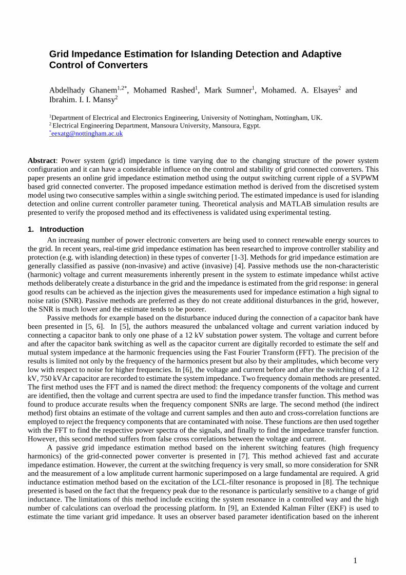
Fig. 2 shows the simulation results for system inductance estimation with different grid impedance parameters.

The grid resistance is changed at t = 0.1 s from 0.113 Ω to 0.5 Ω and the grid inductance is increased at t = 0.2 s from

0.54 mH to 1.43 mH. The results show an accurate estimation of the change in grid inductance (even in the presence

of measurement noise) with insensitivity to resistance variations. The ramp in the estimated inductance is caused by

a rate limit (10 H/s) which has been added to the estimator to reduce the effect of noise and measurement filtering.

Fig. 2-b shows the instants at which the inductance estimation is disabled to avoid the switching instant

ringing/oscillation. Their effect on the inductance estimation process is negligible.

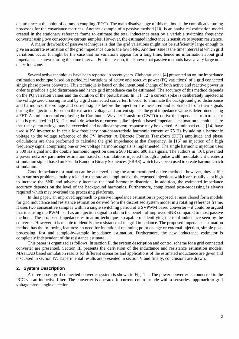
4.2. Islanding detection test

One important application of the grid inductance estimation is islanding detection. A simulation scenario to

show the use of the inductance estimator for islanding detection is given in Fig. 3-a and the results are shown in Fig.

3-b.The converter is connected to a grid made up of two connections; one is strong and the other is weak. The strong

connection in Fig. 4 is disconnected at t = 0.1 s and the estimated inductance changes to a higher value (see Fig. 3-b)

within 50 ms – close to two supply periods. This is fast enough for the change in the estimated inductance to be used

as a flag for islanding.

7

Fig. 2. The estimated inductance for different grid parameters.

a The estimated inductance variation at different grid resistance and inductance.

b Zoom in shows estimation idle instants.

a

b

Fig. 3. Application of the estimated inductance for Islanding.

a Islanding test system configuration.

b Simulation results for islanding detection.

Rgm Lgm

Rf Lf

vdc

VgmPCC

Vc L-Filter

Controller and Inductance

estimator

Rgw Lgw

i conv

i m-g

i w-g

Main Grid

Weak Grid (Loads+DGs)

Vgw

C.B

vdc

8

4.3. Adaptive current control

In this section, the estimated inductance is used for online current control loop tuning. The closed loop transfer

function of the reference current to the actual current is given by:

𝐶(𝑠) =𝐼(𝑠)

𝐼∗(𝑠)=

1

𝐿(𝐾𝐼+𝐾𝑝𝑆)

𝑆2+1

𝐿(𝑅+𝐾𝑝)𝑆+

𝐾𝐼𝐿

(17)

The second order system given by the closed loop transfer function has an undamped natural frequency of 𝜔𝑛 =

√𝐾𝐼 𝐿⁄ and damping ratio of 𝜉 = 0.5√1

𝐾𝐼.𝐿(𝑅 + 𝐾𝑝). The controller parameters Kp and KI are adaptively calculated to

achieve a specific bandwidth and damping ratio based on the estimated inductance. The magnitude of the closed loop

transfer function |𝐶(𝑗𝜔𝑏𝑤)| is set to be -3 dB at the required bandwidth and damping ratio as given by (18, 19).

|𝐶(𝑗𝜔𝑏𝑤)| = [(𝜔𝑏𝑤 𝐾𝑝

𝐿)2

+(𝑅+ 𝐾𝑝

2𝐿𝜉)4

(𝜔𝑏𝑤)2(𝑅+ 𝐾𝑝

𝐿)2

+[(𝑅+ 𝐾𝑝

2𝐿𝜉)2

−(𝜔𝑏𝑤)2]

2]

1/2

=1

√2 (18)

𝐾𝑖 =1

𝐿(𝑅+ 𝐾𝑝

2𝜉)2 (19)

Equation (18) is solved using the Newton-Raphson iterative method for Kp and then Ki is calculated using (19)

to achieve a bandwidth of 200 Hz and damping ratio of 0.8. The adaptive parameters are updated once every sampling

period and the same PI parameters are used for both the d and q current loops.

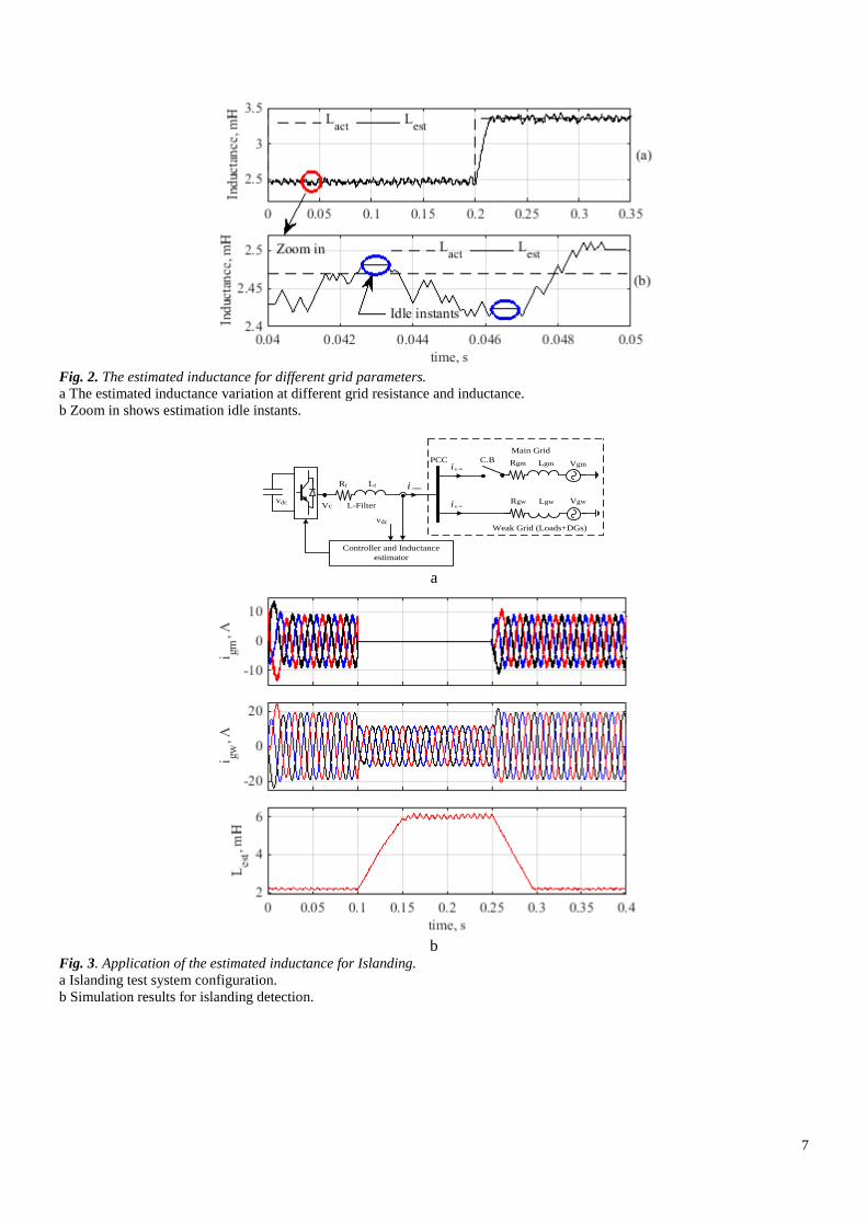
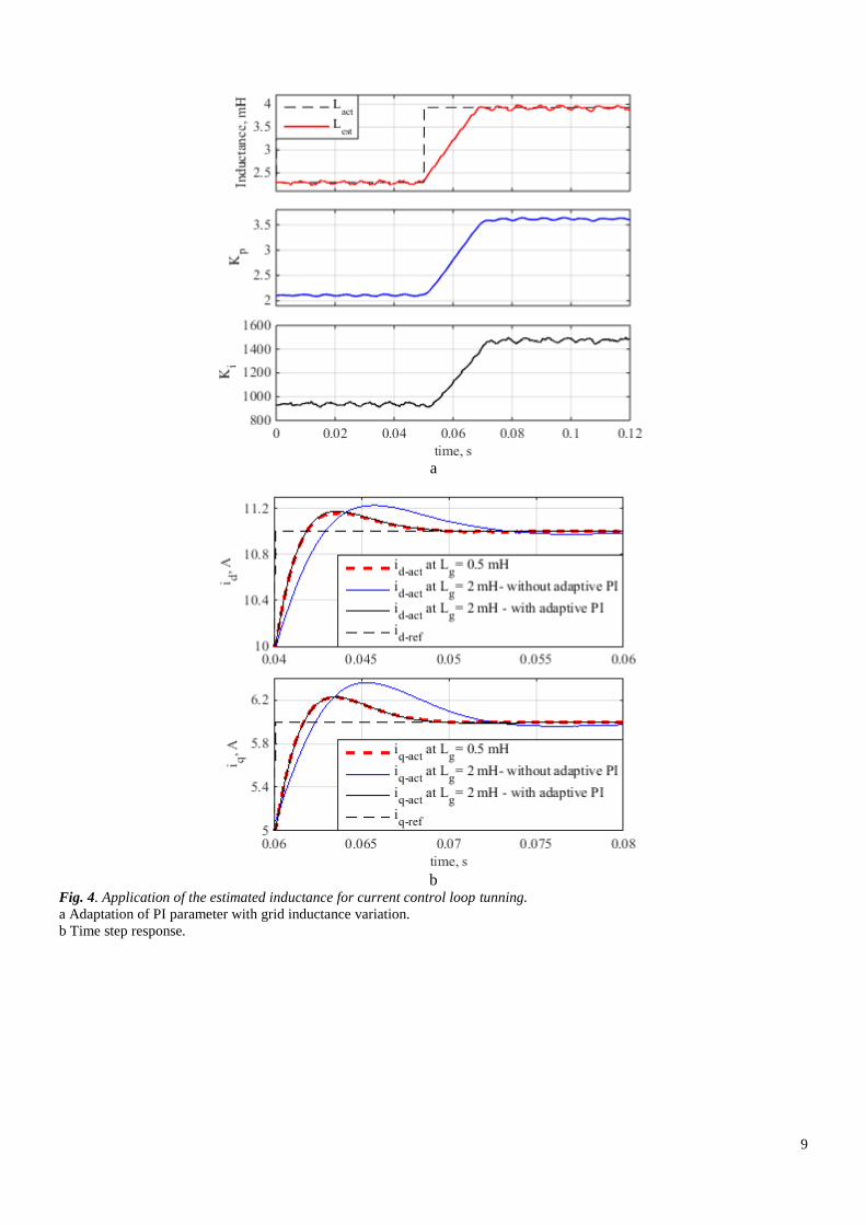
The tuning of the PI parameters due to change of the grid inductance is presented in Fig. 4-a. It can be seen that

at t = 0.05 s the grid inductance is increased to 2 mH giving a total inductance of 3.93 mH. During the change of the

estimated inductance, the PI parameters are also tuned to achieve the specified bandwidth and damping ratio. Once

the new inductance is estimated and becomes constant, the PI parameters also become steady.

The time step response at different grid inductance values without and with the adaptive PI controller for d and

q axes control loops are presented in Fig. 4-b. Obviously, it can be seen that without the PI parameter adaptation, an

increase in the grid inductance affects the performance of the controller and decreases its bandwidth. In contrast, with

the adaptive PI controller, the same step response before and after the grid impedance change is achieved.

5. Experimental Evaluation of Online inductance estimation

An experimental system has been constructed to evaluate the challenges of implementing this impedance

measurement technique on a representative power electronic converter.

The converter controller was implemented using a Texas Instruments TMS320C6713 DSK board alongside

a bespoke Actel FPGA A3P400 based data acquisition board and Host Port Interface (HPI) daughter card for user

interaction. The DSP board has a clock frequency of 225 MHz while the FPGA board has a clock frequency of 50

MHz and has ten channels of Analogue to Digital Converters (ADCs). The dc-side was set at 250 V and the converter

operated in rectifier mode feeding load resistors on the DC side. Note that the tests were performed using switching

frequencies of both 5 kHz and 10 kHz.

The ac supply used for the microgrid was a Chroma 61511 programmable AC source, which can provide an

ideal sinusoidal supply and also harmonic content. An inductive filter is used to connect the converter to PCC, and

two parallel inductors (L1, L2) are used to represent the grid impedance between PCC and the ideal source, as shown

in Fig. 5-a. In addition, a circuit breaker (C.B) is used in series with the inductor L2 in order to switch it in and out of

circuit to vary the grid impedance.

9

a

b

Fig. 4. Application of the estimated inductance for current control loop tunning.

a Adaptation of PI parameter with grid inductance variation.

b Time step response.

10

L-filter

dcv

PCC

Vc

DSP/FPGA

dcvL1

C.B

L2

Grid

Lo

ad

ig

a

b

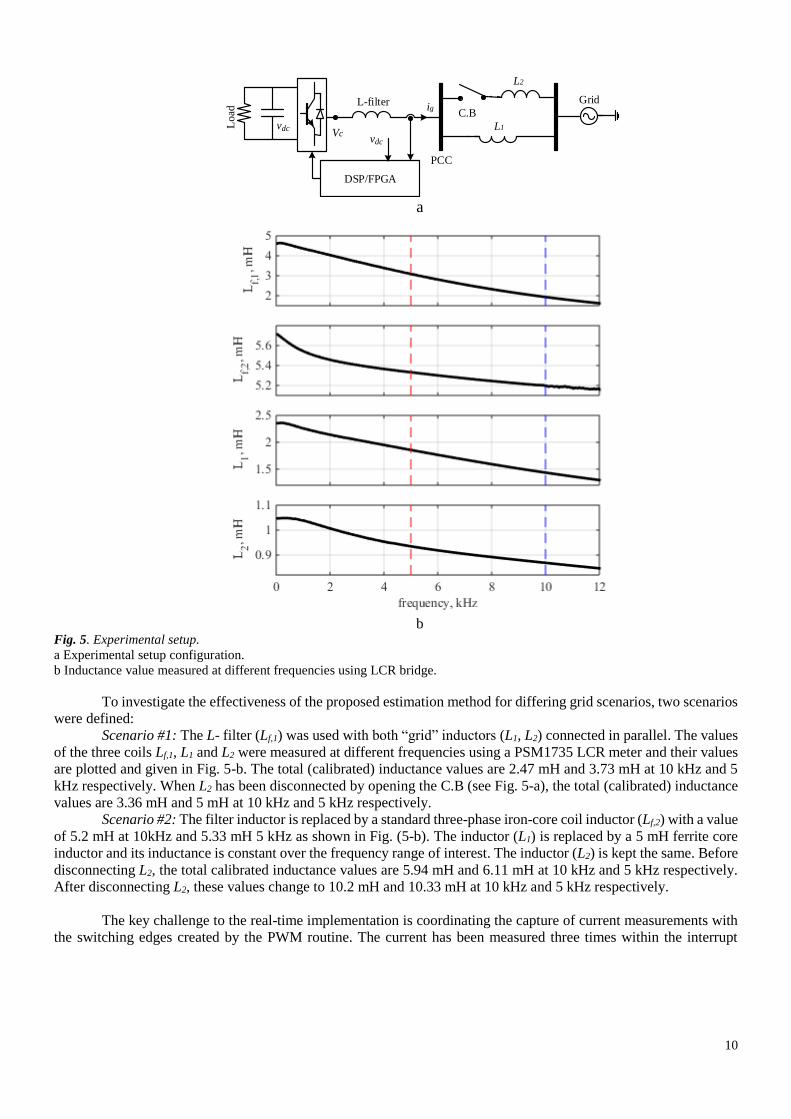
Fig. 5. Experimental setup.

a Experimental setup configuration.

b Inductance value measured at different frequencies using LCR bridge.

To investigate the effectiveness of the proposed estimation method for differing grid scenarios, two scenarios

were defined:

Scenario #1: The L- filter (Lf,1) was used with both “grid” inductors (L1, L2) connected in parallel. The values

of the three coils Lf,1, L1 and L2 were measured at different frequencies using a PSM1735 LCR meter and their values

are plotted and given in Fig. 5-b. The total (calibrated) inductance values are 2.47 mH and 3.73 mH at 10 kHz and 5

kHz respectively. When L2 has been disconnected by opening the C.B (see Fig. 5-a), the total (calibrated) inductance

values are 3.36 mH and 5 mH at 10 kHz and 5 kHz respectively.

Scenario #2: The filter inductor is replaced by a standard three-phase iron-core coil inductor (Lf,2) with a value

of 5.2 mH at 10kHz and 5.33 mH 5 kHz as shown in Fig. (5-b). The inductor (L1) is replaced by a 5 mH ferrite core

inductor and its inductance is constant over the frequency range of interest. The inductor (L2) is kept the same. Before

disconnecting L2, the total calibrated inductance values are 5.94 mH and 6.11 mH at 10 kHz and 5 kHz respectively.

After disconnecting L2, these values change to 10.2 mH and 10.33 mH at 10 kHz and 5 kHz respectively.

The key challenge to the real-time implementation is coordinating the capture of current measurements with

the switching edges created by the PWM routine. The current has been measured three times within the interrupt

11

service routine (ISR) (at the beginning, a quarter and half the way through the switching period). The timing of these

measurements within the interrupt period is achieved using time delay counters. The inductance is calculated every

interrupt period using these three measurements, using the closed form given in (15). A change rate limit is then

applied based on the present and previous value of the calculated inductance in order to alleviate the effect of

measurement noise. The HPI interface daughter card provides a user interface and allows the user to modify and

monitor the parameters within the ISR using the MATLAB environment.

It is worth mentioning that proposed method has been evaluated under ideal and distorted grid voltage

conditions. For the distorted grid, the Chroma output voltage was modified to include five percent of 5th and 7th

harmonic orders.

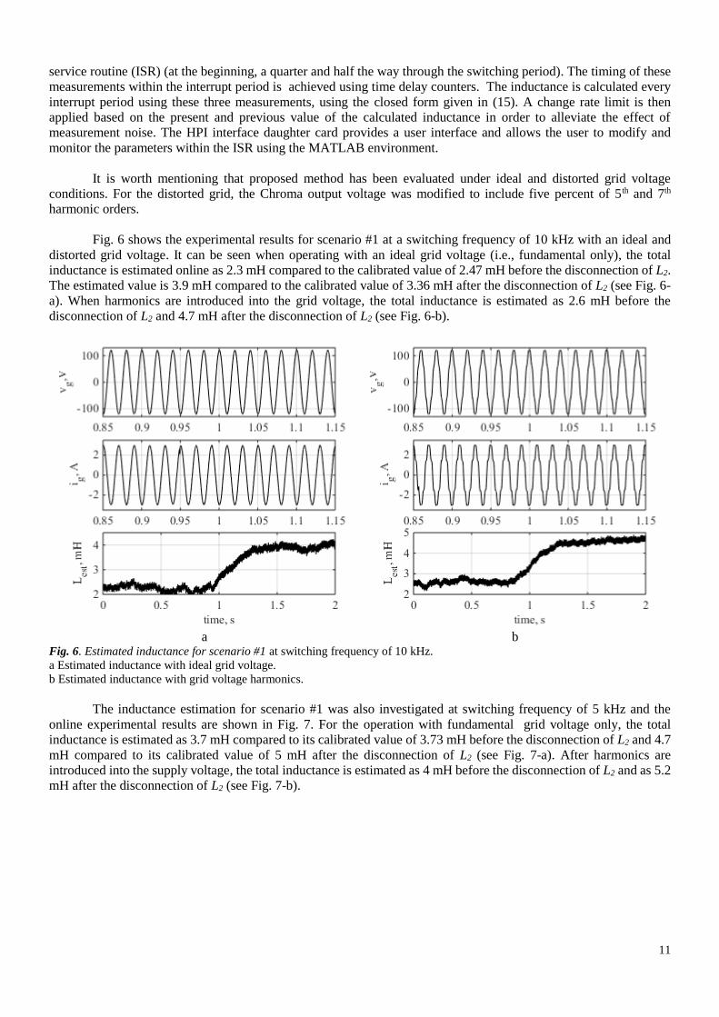
Fig. 6 shows the experimental results for scenario #1 at a switching frequency of 10 kHz with an ideal and

distorted grid voltage. It can be seen when operating with an ideal grid voltage (i.e., fundamental only), the total

inductance is estimated online as 2.3 mH compared to the calibrated value of 2.47 mH before the disconnection of L2.

The estimated value is 3.9 mH compared to the calibrated value of 3.36 mH after the disconnection of L2 (see Fig. 6-

a). When harmonics are introduced into the grid voltage, the total inductance is estimated as 2.6 mH before the

disconnection of L2 and 4.7 mH after the disconnection of L2 (see Fig. 6-b).

a b

Fig. 6. Estimated inductance for scenario #1 at switching frequency of 10 kHz.

a Estimated inductance with ideal grid voltage.

b Estimated inductance with grid voltage harmonics.

The inductance estimation for scenario #1 was also investigated at switching frequency of 5 kHz and the

online experimental results are shown in Fig. 7. For the operation with fundamental grid voltage only, the total

inductance is estimated as 3.7 mH compared to its calibrated value of 3.73 mH before the disconnection of L2 and 4.7

mH compared to its calibrated value of 5 mH after the disconnection of L2 (see Fig. 7-a). After harmonics are

introduced into the supply voltage, the total inductance is estimated as 4 mH before the disconnection of L2 and as 5.2

mH after the disconnection of L2 (see Fig. 7-b).

12

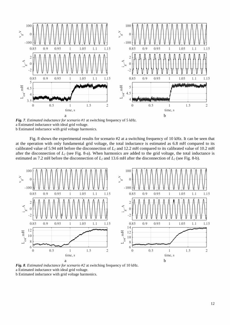
a b




Fig. 8 shows the experimental results for scenario #2 at a switching frequency of 10 kHz. It can be seen that

at the operation with only fundamental grid voltage, the total inductance is estimated as 6.8 mH compared to its

calibrated value of 5.94 mH before the disconnection of L2 and 12.2 mH compared to its calibrated value of 10.2 mH

after the disconnection of L2 (see Fig. 8-a). When harmonics are added to the grid voltage, the total inductance is

estimated as 7.2 mH before the disconnection of L2 and 13.6 mH after the disconnection of L2 (see Fig. 8-b).

a b




13

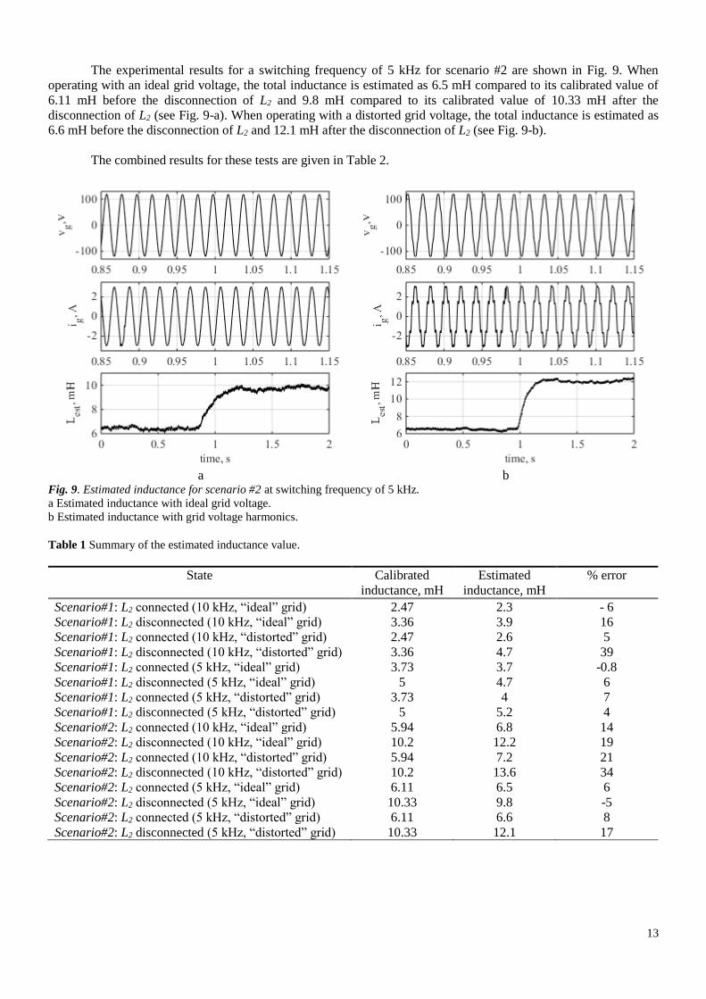
The experimental results for a switching frequency of 5 kHz for scenario #2 are shown in Fig. 9. When

operating with an ideal grid voltage, the total inductance is estimated as 6.5 mH compared to its calibrated value of

6.11 mH before the disconnection of L2 and 9.8 mH compared to its calibrated value of 10.33 mH after the

disconnection of L2 (see Fig. 9-a). When operating with a distorted grid voltage, the total inductance is estimated as

6.6 mH before the disconnection of L2 and 12.1 mH after the disconnection of L2 (see Fig. 9-b).

The combined results for these tests are given in Table 2.

a b




Table 1 Summary of the estimated inductance value.

State Calibrated

inductance, mH

Estimated

inductance, mH

% error

Scenario#1: L2 connected (10 kHz, “ideal” grid) 2.47 2.3 - 6

Scenario#1: L2 disconnected (10 kHz, “ideal” grid) 3.36 3.9 16

Scenario#1: L2 connected (10 kHz, “distorted” grid) 2.47 2.6 5

Scenario#1: L2 disconnected (10 kHz, “distorted” grid) 3.36 4.7 39

Scenario#1: L2 connected (5 kHz, “ideal” grid) 3.73 3.7 -0.8

Scenario#1: L2 disconnected (5 kHz, “ideal” grid) 5 4.7 6

Scenario#1: L2 connected (5 kHz, “distorted” grid) 3.73 4 7

Scenario#1: L2 disconnected (5 kHz, “distorted” grid) 5 5.2 4

Scenario#2: L2 connected (10 kHz, “ideal” grid) 5.94 6.8 14

Scenario#2: L2 disconnected (10 kHz, “ideal” grid) 10.2 12.2 19



Scenario#2: L2 connected (5 kHz, “ideal” grid) 6.11 6.5 6

Scenario#2: L2 disconnected (5 kHz, “ideal” grid) 10.33 9.8 -5



14

It is clear from Figs. 6 to 8 that the grid inductance estimator can identify changes in supply impedance when

implemented in an experimental system. However it is also clear from Table 2 that the error in the estimation is

dependent on operating conditions and is certainly higher than seen in the simulation studies. There are significant

differences between the simulation and experimental systems: measurement noise is more prominent, especially as

the measurements used are taken close to the switching of power converters; the timing of the measurements is

dependent on both the resolution of the system clock and the interrupt latency associated with the measurement time

and errors in these timings can have a large effect on the accuracy of the non-averaged terms of (15). Other real

phenomena such as semiconductor nonlinearities, device voltage drop, dead time, antialiasing filters and current

sensor accuracy will all influence the behaviour of this estimator.

For example, the results of Table 2 show that the proposed inductance estimator has improved accuracy when

employed at a lower switching frequency. This is likely to be due to the increased amplitude of the current ripple

(even when the grid voltage is distorted) which reduces the effect of measurement noise and improves the resolution.

The lower switching frequency will also reduce the influence of timing delays in the sampling and PWM processes.

More investigation is required to determine the relative influences of these phenomena on the accuracy of the

identification algorithm. However, even in this early experimental implementation the proposed inductance estimator

can effectively detect the variation of inductance even with a distorted grid voltage.

6. Conclusion

Closed-form grid inductance and resistance estimation models have been derived from the discrete grid

connected converter modelled in the dq reference frame. The estimators use two consecutive current samples

measured within a single SVPWM switching period. The derived inductance and resistance estimator models are fully

decoupled and independent. The effectiveness of the proposed estimation approach for islanding detection and

adaptive tuning (online) of the PI current controller gains have verified by simulation even in the presence of

representative measurement noise. Experimental results demonstrate that the proposed impedance estimator can detect

changes in grid impedance although its accuracy is lower than expected. The proposed method has been shown to be

more effective when a low switching frequency is used. It is thought that the lower accuracy in the experimental

system is due to errors in the timing of the measurements made in the experimental system: the accuracy improves as

the switching period becomes higher and the influence of timing errors reduces. Future work will investigate this

further. Other applications of the proposed method include converters for motor drives which use an L-only filter or

that connect directly to the machine e.g., permanent magnet synchronous machine drives. Furthermore, it can be as

the basis of a portable device to measure the grid inductance at specific network positions.

7. References

[1] Guo, X.Q., Zhang, X., Wang, B.C., et al.:‘Asymmetrical grid fault ride-through strategy of three-phase grid-connected

inverter considering network impedance impact in low-voltage grid’, IEEE Transactions on Power Electronics, 2014, 29,

(3), pp. 1064-1068

[2] Strasser, T., Andren, F., Kathan, J., et al.:‘A review of architectures and concepts for intelligence in future electric energy

systems’, IEEE Transactions on Industrial Electronics, 2015, 62, (4), pp. 2424-2438

[3] Sumner, M., Abusorrah, A., Thomas, D., et al.:‘Real time parameter estimation for power quality control and intelligent

protection of grid-connected power electronic converters’, IEEE Transactions on Smart Grid, 2014, 5, (4), pp. 1602-1607

[4] Ciobotaru, M., Teodorescu, R., Rodriguez, P., et al.:‘Online grid impedance estimation for single-phase grid-connected

systems using PQ variations’, in, 2007 IEEE Power Electronics Specialists Conference, 2007

[5] Crevier, D. and Mercier, A.:‘Estimation of Higher Frequency Network Equivalent Impedances by Harmonic Analysis

Natural Waveforms’, IEEE Transactions on Power Apparatus and Systems, 1978, PAS-97, (2), pp. 424-431

[6] Girgis, A.A. and McManis, R.B.:‘Frequency domain techniques for modeling distribution or transmission networks using

capacitor switching induced transients’, IEEE Transactions on Power Delivery, 1989, 4, (3), pp. 1882-1890

[7] Herong, G., Guo, X., Deyu, W., et al.:‘Real-time grid impedance estimation technique for grid-connected power

converters’, in, Industrial Electronics (ISIE), 2012 IEEE International Symposium on, 2012

[8] Liserre, M., Blaabjerg, F., and Teodorescu, R.:‘Grid impedance estimation via excitation of LCL-filter resonance’, IEEE

Transactions on Industry Applications, 2007, 43, (5), pp. 1401-1407

15

[9] Hoffmann, N. and Fuchs, F.W.:‘Minimal invasive equivalent grid impedance estimation in inductive-resistive power

networks using extended kalman filter’, IEEE Transactions on Power Electronics, 2014, 29, (2), pp. 631-641

[10] Arif, B., Tarisciotti, L., Zanchetta, P., et al.:‘Grid parameter estimation using model predictive direct power control’, IEEE

Transactions on Industry Applications, 2015, 51, (6), pp. 4614-4622

[11] Cespedes, M. and Sun, J.:‘Online grid impedance identification for adaptive control of grid-connected inverters’, in, 2012

IEEE Energy Conversion Congress and Exposition (ECCE), 2012

[12] Palethorpe, B., Sumner, M., and Thomas, D.W.P.:‘Power system impedance measurement using a power electronic

converter’, in, Harmonics and Quality of Power, 2000. Proceedings. Ninth International Conference on, 2000

[13] Sumner, M., Thomas, D.W.P., and Zanchetta, P.:‘Power System Impedance Estimation for Improved Active Filter Control,

using Continuous Wavelet Transforms’, in, 2005/2006 IEEE/PES Transmission and Distribution Conference and

Exhibition, 2006

[14] Asiminoaei, L., Teodorescu, R., Blaabjerg, F., et al.:‘Implementation and test of an online embedded grid impedance

estimation technique for PV inverters’, IEEE Transactions on Industrial Electronics, 2005, 52, (4), pp. 1136-1144

[15] Ciobotaru, M., Teodorescu, R., and Blaabjerg, F.:‘On-line grid impedance estimation based on harmonic injection for grid-

connected PV inverter’, in, 2007 IEEE International Symposium on Industrial Electronics, 2007

[16] Neshvad, S., Chatzinotas, S., and Sachau, J.:‘Wideband identification of power network parameters using pseudo-random

binary sequences on power inverters’, IEEE Transactions on Smart Grid, 2015, 6, (5), pp. 2293-2301

[17] Zhou, J.Z., Ding, H., Fan, S.T., et al.:‘Impact of short-circuit ratio and phase-locked-loop parameters on the small-signal

behavior of a VSC-HVDC converter’, IEEE Transactions on Power Delivery, 2014, 29, (5), pp. 2287-2296

[18] Li, D., Notohara, Y., Iwaji, Y., et al.:‘AC voltage and current sensorless control method for three‐phase PWM

converter’, Electrical Engineering in Japan, 2010, 172, (4), pp. 48-57

[19] Shu, Z.L., Tang, J., Guo, Y.H., et al.:‘An efficient SVPWM algorithm with low computational overhead for three-phase

inverters’, IEEE Transactions on Power Electronics, 2007, 22, (5), pp. 1797-1805

[20] Siwakoti, Y.P. and Town, G.E.:‘Design of FPGA-controlled power electronics and drives using MATLAB simulink’, in,

ECCE Asia Downunder (ECCE Asia), 2013 IEEE, 2013

[21] Ginart, A.E., Brown, D.W., Kalgren, P.W., et al.:‘Online ringing characterization as a diagnostic technique for IGBTs in

power drives’, IEEE Transactions on Instrumentation and Measurement, 2009, 58, (7), pp. 2290-2299

grid impedance estimation for islanding detection and ...eprints.nottingham.ac.uk/44087/1/grid...

Documents