grid modernization: metrics analysis (gmlc1.1) 1_reference... · iii executive summary this report...
TRANSCRIPT

PNNL-26541
Grid Modernization: Metrics Analysis (GMLC1.1)
Reference Document, Version 2.1
May 2017
Grid Modernization Laboratory Consortium


PNNL-26541
Grid Modernization: Metrics Analysis (GMLC1.1)
Reference Document Version 2.1
Grid Modernization Laboratory Consortium Members: David Anderson1 Michael Kintner-Meyer
1
Annika Eberle7 Julia Phillips
4
Thomas Edmunds2 Gian Porro
7
Joseph Eto3 Monisha Shah7
Steven Folga4 Cesar Silva-Monroy5 Stan Hadley6 Eric Vugrin
5
Garvin Heath7 Meng Yue8
Angeli Tompkins4
May 2017
Prepared for the U.S. Department of Energy under Contract DE-AC05-76RL01830
Pacific Northwest National Laboratory Richland, Washington 99352
1 Pacific Northwest National Laboratory
2 Lawrence Livermore National Laboratories
3 Lawrence Berkeley National Laboratory
4 Argonne National Laboratory
5 Sandia National Laboratories
6 Oak Ridge National Laboratory
7 National Renewable Energy Laboratory
8 Brookhaven National Laboratory


iii
Executive Summary
This report is version 2.1 of the Reference Document for the Grid Modernization Laboratory Consortium
(GMLC) Metrics Analysis project , generally referred to by its initials, GMLC1.1. It documents the
progress made after Year 1 of conducting the project to select, describe, and define metrics for the
purpose of monitoring and tracking system properties of the electric infrastructure as it evolves over time.
The Reference Document covers the following six topic areas for characterizing the U.S. electric grid:
Reliability Sustainability
Resilience Affordability
Flexibility Security
These six topics were selected by the U.S. Department of Energy (DOE) as a core set of electric
infrastructure metrics areas that are important to track (DOE 2015a). No claim has been made about the
completeness of this set, but it appears that the six areas are a reasonable starting point for a metrics
analysis.
The expected outcome of this 3-year GMLC Metrics Analysis project is to enhance the existing state of
metrics to 1) provide federal, state, and municipal regulators more comprehensive information about the
current state of the electricity system to measure impacts of grid modernization and technology
deployment, 2) support self-assessment by utility organizations across multiple attributes of grid
operations, and 3) enable DOE to better set priorities on modernization research and development (R&D).
To achieve this outcome, the project team adopted the following approach: 1) engage with key
stakeholders and data partners in each of the six metrics areas to understand industry needs, data
availability, access to data, and potential use of metrics and concerns about misuse of metrics results; 2)
define new metrics or enhancements to existing metrics; 3) validate metrics in real-world conditions; and
4) work on the adoption of metrics through standards bodies or use by key data partners.
Definitions of Metrics
The six metric categories explored in this project are described in Table 1.1.
Table ES.1. Metrics Descriptions and Focus Areas
Attribute Definition Existing Metrics Metrics Being Refined or
Developed
Reliability: Maintain the delivery
of electric services to customers in
the face of routine uncertainty in
operating conditions.
For utility distribution systems,
measuring reliability focuses on
interruptions in the delivery of
electricity in sufficient quantities
and of sufficient quality to meet
electricity users’ needs for (or
Existing reliability metrics
(e.g., SAIDI and SAIFI),
though mature, pertain
primarily to distribution
networks. They gauge the
frequency and duration of
outages averaged over all
customers within a given
service territory over a
specified time period. This
At the distribution level, the GMLC analysts
are developing more granular, value-based
metrics that will enable utilities to estimate
the likely costs to customers of outages in
specific locations so that investment dollars
can be allocated to reduce the likelihood of
the most costly interruptions. These metrics
will be developed and demonstrated through
a partnership with the American Public
Power Association.

iv
Attribute Definition Existing Metrics Metrics Being Refined or
Developed
applications of) electricity. For the
bulk power system, measuring
reliability focuses separately on
both the operational (current or
near-term conditions) and
planning (longer-term) time
horizons.
approach masks the wide
variance among outages in
terms of size, duration, and
economic impact on
customers.
At the bulk power level, the GMLC team
will work with NERC on new transmission
metrics to gauge the overall health (in terms
of reliability) of three North American
interconnections.
Resilience: “The ability to
prepare for and adapt to changing
conditions and withstand and
recover rapidly from disruptions.
Resilience includes the ability to
withstand and recover from
deliberate attacks, accidents, or
naturally occurring threats or
incidents.”1
At present, widely-accepted
metrics for resiliency do not
exist. As noted above, existing
reliability metrics do not focus
on the impacts resulting from
individual events or on
individual critical sectors,
especially resilience events,
which are infrequent, yet have
large consequences.
GMLC analysts are piloting new metrics
through case studies of hypothetical
resilience conducted with industry
stakeholders (e.g., City of New Orleans
facing another Category 5 hurricane)
Direct metrics
Electrical
Service
Cumulative customer-
hours of outages
Cumulative customer
energy demand not
served
Average number (or
percentage) of
customers experiencing
an outage during a
specified time period
Critical
Electrical
Service
Cumulative critical
customer-hours of
outages
Critical customer
energy demand not
served
Average number (or
percentage) of critical
loads that experience an
outage
Restoration Time to recovery
Cost of recovery
Monetary Loss of utility revenue
Cost of grid damages
(e.g., repair or replace
lines, transformers)
Cost of recovery
Avoided outage cost
Indirect metrics
Community Critical services
1 Source: Presidential Policy Directive 21 [PPD-21, Obama 2013]

v
Attribute Definition Existing Metrics Metrics Being Refined or
Developed
Function without power (e.g.,
hospitals, fire stations,
police stations)
Flexibility: The ability of the grid
(or a portion of it) to respond to
future uncertainties that stress the
system in the short term and may
require the system to adapt over
the long term. Two perspectives:
1) from an operational viewpoint,
the agility of the electrical
network in adjusting to known or
unforeseen short-term changes,
such as abrupt changes in load
conditions or sharp ramps due to
errors in renewable generation
forecasts; and 2) from a strategic
investment perspective, the ability
to respond to major regulatory and
policy changes and technological
breakthroughs without incurring
stranded assets.
At present, widely-accepted
metrics for flexibility do not
exist.
Grid operators have told GMLC analysts
that the flexibility metrics they need most
urgently pertain to coping with short-term
fluctuations in the availability of generation
from wind and utility-scale solar facilities.
The analysts are evaluating more than 20
separate metrics that could be used to either
understand quickly the nature of a given
fluctuation or to estimate the likely
effectiveness of alternative options for
dealing with a particular fluctuation.
The GMLC analysts are concentrating on
this bulk-power problem and have deferred
for a later time the issues of how to measure
and respond to short-term flexibility
challenges at the distribution level, and how
to build more flexibility into long-term
system plans.
Sustainability: The provision of
electric services to customers
while minimizing negative
impacts on humans and the natural
environment. This attribute may
be more broadly defined as
including three pillars:
environmental, social, and
economic. GMLC is focusing first
on the environmental pillar.
A wealth of existing and
mature metrics exists,
particularly regarding
electricity-related
environmental impacts.
However, most of these
metrics pertain to “ lagging”
indicators, as opposed to
metrics that would aid in
predicting likely future
performance.
The GMLC analysts are focusing first on
how to aid stakeholders in making better use
of the available information related to
greenhouse gas (GHG) emissions, including
identification of current gaps in available
information (e.g. emissions from distributed
generation). In the second year of this three-
year study, the GMLC analysts will develop
a new metric to better quantify the
relationship between power sector water use
and water availability in affect ed areas.
Affordability: The ability of the
system to provide electric services
at a cost that does not exceed
customers’ willingness and ability
to pay for those services.
Several mature metrics exist
pertaining to the cost-
effectiveness of alternative
investments in specific
technologies, services,
practices, or regulations.
Examples include calculation
of the levelized cost of
electricity (LCOE) from new
or existing generators, and the
internal rate of return (IRR) for
The GMLC analysts are focusing primarily
on demonstrating the applicability of
customer cost-burden metrics to investment-
related options that are evaluated at the
utility, state, and national levels. They are
also collaborating with another team of
GMLC analysts to demonstrate the value of
cost-burden metrics in the conduct of the
Alaska Microgrid Project, which is
designing renewable-based microgrids for
two remote Alaskan villages. The purpose

vi
Attribute Definition Existing Metrics Metrics Being Refined or
Developed
many kinds of grid-related
investments or combinations of
them.
Metrics are evolving but are
not yet widely accepted for
gauging the relative size of the
“ cost burden” that paying for
electricity services represents
for customers. Most work in
this area has focused on low-
income residential customers.
Very little work has been done
pertaining to cost burden for
commercial and industrial
customers.
of the microgrids is to reduce the extreme
cost of providing electricity services to these
communities using petroleum-based fuels
delivered by aircraft.
Security: The ability to resist
external disruptions to the energy
supply infrastructure caused by
intentional physical or cyber
attacks or by limited access to
critical materials from potentially
hostile countries. GMLC is
focusing first on external
disruptions to electricity supply
infrastructure.
Although a variety of metrics
have been proposed, at present
widely-accepted metrics for
security do not exist.
Development and application
of metrics for this attribute is
difficult because there are no
actuarial tables that can tell
what adversaries are likely to
do, how often they will do it,
and how much it will cost the
electricity sector when they do
it. Further, the subject does
not lend itself to modeling
because of the large number of
unknowns that would have to
be estimated and the large
margin of error associated with
those unknowns.
The Department of Homeland Security
(DHS) has developed an Infrastructure
Survey Tool (IST) that can be used to
collect physical security information
pertaining to a given facility. The
information thus gathered can then be
compiled into a metric called the Protective
Measures Index (PMI). The IST/PMI
method is applicable to many kinds of
energy facilities. GMLC analysts are
revising and refining the IST/PMI method to
make it more electricity specific. They are
demonstrating the modified method with
electric-sector organizations (e.g.,
Commonwealth Edison) through field tests.
Note that this effort pertains only to
assessing the physical security of grid
facilities. The GMLC analysts will address
cyber security in a subsequent stage of this
three-year project.
Stakeholder Engagement
Throughout the project, input and feedback are sought out from stakeholders. Key national organizations
in the electric industry were identified as Working Partners at the inception of the project and engaged to

vii
provide both strategic and technical input to the project as a whole. Three types of organizations were a lso
identified for each of the six individual metric areas: (1) primary metric users, (2) subject matter experts,
and (3) data or survey organizations. These stakeholders were engaged at various stages of the project,
especially at, but not limited to, the beginning and scoping stages of the effort and then to more formally
review the content in this document at the end of Year 1.
The project team engaged with, received feedback from, and in some cases, formed a partnership with the
following entities:
Reliability: North American Electric Reliability Corporation (NERC), Institute of Electrical and
Electronics Engineers (IEEE), American Public Power Association (APPA),
Resilience: DOE/Office of Energy Policy and Systems Analysis (DOE/EPSA), U.S. Department of
Homeland Security (DHS), City of New Orleans, PJM Interconnection, Electric Power
Research Institute (EPRI)
Flexibility: Federal Energy Regulatory Commission (FERC), Pacific Gas and Electric Company
(PG&E), California Independent System Operator (CAISO), EPRI, Electric Reliability
Council of Texas, Inc. (ERCOT)
Sustainability: U.S. Environmental Protection Agency (EPA), Energy Information Administration
(EIA), Arizona State University National Resources Research Institute (NRRI),
Sustainability Accounting Standards Board (SASB)
Affordability: EPRI, Minnesota Public Utilities Commission (PUC), Colorado State Energy Office,
Washington State Utilities and Transportation Commission (UTC), Nation Association of
Regulatory Utility Commissioners (NARUC), Alaska Energy Authority
Security: DHS, EPRI, National Association of State Energy Officials (NASEO), Edison Electric
Institute (EEI), Exelon Corporation.
Below is a summary of the feedback from partners regarding the value of the specific metrics
development.
New Metrics Development
Definition
Metrics are discussed by their ability to characterize system properties measured in the past ( lagging
metrics) as well as metrics that represent the system’s ability to respond to challenges in the future
(leading metrics).
Reliability
Reliability refers to maintaining the delivery of electric power to customers in the face of routine
uncertainty in operating conditions. For utility distribution systems, measuring reliability focuses on
interruption in the delivery of electricity in sufficient quantities and of sufficient quality to meet
electricity users’ needs for (or applications of) electricity. For the bulk power system, measuring
reliability focuses separately on both the operational (current or near -term conditions) and planning
(longer-term) time horizons.

viii
GMLC1.1 focuses on the following three thrusts within the reliability metrics area:
Improving distribution system metrics
Improving transmission system metrics
Probabilistic enhancement of transmission planning metrics.
Improvements in reliability metric designs are needed to better link metrics to the value of reliability; e.g.,
the economic costs borne by customers (and utilities) when power is interrupted. Examining these costs
involves analyzing informat ion on individual interruptions that is more granular than the information
summarized in traditional metrics for annual reliability performance. That is, information is needed on
which customers have lost power and for how long. The utilization of this kin d of information is essential
for introducing economic considerations into grid modernization decisions, so that decision -makers can
determine how much improving reliability is worth to a utility, its customers, and society at large.
In addition, research into new metrics is needed. For example, transmission metrics for the overall health
(from a reliability standpoint) of the three U.S. Interconnections each taken as a whole, have only recently
been formulated by NERC’s Performance Analysis Subcommittee. Research is needed to help make them
even more useful in guiding public and private decision -making.
Currently, the project is working on the improvement of distribution system metrics. The remaining two
thrusts are planned activities for Years 2 and 3.
Existing, lagging metrics of distribution reliability (e.g., SAIDI and SAIFI) represent aggregations of
interruptions averaged over all customers within a service territory. Consequently, they suppress
information that is of growing importance for supporting improvements in the planning and operation of
distribution systems. This information, which utilities already collect, involves assessing which types of
customers (residential, commercial, industrial) have experienced a power interruption and for how long in
order to understand the economic costs that power interruptions impose on them. This task is being
conducted in partnership with the American Public Power Association. It will develop new metrics that
enable direct consideration of the cost of power int erruptions to customers that will support future
distribution system planning and operating decisions.
Resilience
The Presidential Policy Directive 21 [PPD-21] (Obama 2013) asserts the following definition of
resilience:
The term ‘resilience’ means the ability to prepare for and adapt to changing conditions and
withstand and recover rapidly from disruptions. Resilience includes the ability to withstand and
recover from deliberate attacks, accidents, or naturally occurring threats or incidents.
PPD-21 establishes a national policy on critical infrastructure resilience; additionally, PPD-21’s resilience
definition is consistent with most other proposed definitions (e.g., Biringer et al. 2013).
The project has developed a set of grid resilience metrics and a process for calculating them. The metrics
and process have been developed to accomplish the following:
Help utilities better plan for and respond to low-probability, high-consequence disruptive events that
are not currently addressed in reliability metrics and analyses.
Provide an effective, precise, and consistent means for utilities and regulators to communicate about
resilience issues.

ix
The proposed resilience metrics are leading indicators with a forward look at estimating or projecting the
resilience of the electric infrastructure given a certain threat scenario.
The GMLC1.1 team recommends that grid resilience metrics be consequence-based and, to the extent
possible, they should be reflective of the inherent uncertainties that drive response and plann ing activities.
Table ES.2 lists example consequence categories to serve as the basis for resilience metrics. All of the
consequence categories are measured for the defined system specifications and therefore may be
measured across spatial (geographical) and temporal (duration) dimensions.
Table ES.2. Examples of consequence categories for consideration in grid resilience metric
development.
Consequence Category Resilience Metric
Direct
Electrical Service Cumulative customer-hours of outages
Cumulative customer energy demand not served Average number (or percentage) of customers experiencing an outage during a
specified time period
Critical Electrical Service Cumulative critical customer-hours of outages
Critical customer energy demand not served
Average number (or percentage) of critical loads that experience an outage
Restoration Time to recovery
Cost of recovery
Monetary Loss of utility revenue
Cost of grid damages (e.g., repair or replace lines, transformers)
Cost of recovery
Avoided outage cost
Indirect
Community Function Critical services without power (e.g., hospitals, fire stations, police stations) Critical services without power for more than N hours (where backup power
exists by outage exceeds fuel supply, i.e., N > hours of backup fuel requirement)
Monetary Loss of assets and perishables
Business interruption costs
Impact on Gross Municipal Product (GMP) or Gross Regional Product (GRP)
Other critical assets Key production facilities without power
Key military facilities without power
The project team recommends the following Resilience Analysis Process (RAP), originally developed by
Watson et al. (2015) for the 2015 Quadrennial Energy Review (QER). The RAP (Figure ES.1) illustrates
the seven-step process to be used to help specify resilience objectives for utilities.

x
Figure ES.1. The Resilience Analysis Process.
The seven steps are further defined as follows:
1. Define resilience goals. The goals lay the foundation for all following steps. For example, the
specific goal could be to assess the resilience of a power system to a previous historical event .
Alternatively, the goal could be to evaluate possible system improvements. System specification (e.g.,
geographic boundaries, physical and operational components, relevant time periods, etc.) is required.
2. Define consequence categories and resilience metrics. In the context a specified hazard, the RAP
measures the resilience of a power system by quantifying the consequences of the hazard for the
power system and other infrastructures and communities that depend upon the power system. The
consequence categories should reflect the resilience goals. Resilience analyses are not restricted to a
single consequence category when developing metrics
3. Characterize hazards. Hazard characterization involves the specification of hazards of concern (e.g.,
hurricane, cyber-attack, etc.). Development of hazard scenarios includes detailing the specific hazard
conditions—for instance, frequency or probability of occurrence, the expected hurricane trajectory,
wind speeds, regions with storm surge and flooding, landfall location, duration of the event, and other
conditions—needed to sufficiently characterize the hazard and its potential impact on the power
system.
4. Determine the level of disruption. This step specifies the level of damage or stress that grid assets
are anticipated to suffer under the specified hazard scenarios. For example, anticipated physical
damage (or a range of damage outcomes when incorporating uncertainty) to electric grid assets from a
hurricane hazard might include substation X is nonfunctional because of being submerged by sea
water, lines Y and Z are blown down due to winds, etc.
5. Collect consequence data via system model or other means. Utilities maintain Outage
Management Systems (OMSs). These systems are often a rich source of data for resilience analyses,
though for the largest events, they often lack details such as the actual locations of the causes of the
individual outages and information about system design and condition. When conducting forward-
looking analyses, system-level computer models can provide the necessary power disruption
estimates. These models use the damage estimates from the previous RAP step as inputs to project
how delivery of power will be disrupted. Multiple system models may be required to capture all of
the relevant aspects of the complete system.
6. Calculate consequences and resilience metrics. Most energy systems provide energy for some
larger social purpose (e.g., transportation, healthcare, manufacturing, economic gain). During this

xi
step, outputs from system models are converted to the resilience metrics that were defined during
Step 2.
7. Evaluate resilience improvements. After developing a baseline for resilience quantification by
completing the preceding steps, it is possible and desirable to populate the metrics for a system
configuration that is in some way different from the baseline in order to compare which configuration
would provide better resilience. This could be a physical change (e.g., adding a redundant power
line); a policy change (e.g., allowing the use of stored gas reserves during a disruption); or a
procedural change (e.g., turning on or off equipment in advance of a storm).
Some examples from recent Superstorm Sandy were developed to illustrate the application of the RAP
process.
Flexibility
Grid flexibility refers to the ability to respond to future uncertainties that may stress the system in the
short term and require the system to adapt over the long term . System flexibility can be defined from two
perspectives: 1) from an operational viewpoint that considers the agility of the electric al network to adjust
to known or unforeseen changes, for instance in load conditions or responding to sharp ramps due to error
in renewable generation forecasts; and 2) flexibility from a strategic investment perspective that would
consider the flexibility in expansion planning to respond to new regulatory and policy changes as well as
to technological breakthroughs without incurring stranded assets. GMLC1.1 focuses on the former—the
operational system agility.
The scope of flexibility metric development has been limited to the bulk power system solely based on
the urgency that RTOs/Independent System Operators (ISOs) have expressed about needing a better
understanding of the flexibility requirements to address expected increases in generation fluctuations from
wind and utility-scale solar installations. The flexibility concerns for distribution systems have not risen
to the same level of urgency as the concerns mentioned by grid operators of the transmission network.
However, with increasing distributed energy resource penetration, flexibility concerns may arise for
distribution systems as well. Currently, “hosting capacities” for rooftop photovoltaic installations of
individual feeders are being used as an indicator to assess the need for feeder upgrades. If and when we
reach increasing limitations of hosting capacity, the exploration of flexibility metrics for the distribution
system will become more compelling and urgent.
The motivation to consider operational flexibility stems from the need to accommodate an increasing
amount of variable generation from renewable resources (solar, wind), and the fact that an inflexible
system can lead to lower reliability, higher costs, and lower sustainability (as expressed in higher
emissions or higher consumptive use of water resources) . In this report, we focus on both lagging and
leading indicators.
The set of potential new flexibility metrics for use directly in operations and in planning models to
estimate future flexibility requirements is large and currently under investigation. They include the
following:
1. Loss of load 2. Insufficient
ramping
3. Flexibility ratio 4. Wind generation
5. Solar generation
fraction
6. Wind generation
volatility
7. Solar generation
volatility
8. Net load
forecasting error
9. Net load factor 10. Maximum ramp
rate in net load
11. Maximum ramp
capacity
12. Energy storage
available
13. Demand response 14. Inter-regional 15. Intra-regional 16. Interruptible tariffs

xii
capability transfer capability transfer capability
17. Renewable
curtailment
18. Negative LMP 19. Price spikes 20. Load shedding
21. Operational reserve
shortage
22. Control
performance (CPSs
1. 2; BAAL)
23. Out-of-market
operations
(BAAL = Balancing Authority area control limit; CPS = Control Performance Standard; LMP = Locational
marginal price)
The metrics can be used individually and in combination to infer causality and to inform system planning
decisions and operating policies. For example, if a wind curtailment occurs coincident with a large net
load forecast error, the lack of flexibility could be attributed to forecast accuracy rather than insufficient
ramping capability in the system.
The project team has developed a process to down-select the 23 candidates to a small set. It is recognized
that not all metrics are universally applicable for all stakeholders; the metric down-selection process will
be driven by stakeholders engaged in the use cases (CAISO, ERCOT, or both). Because CAISO has a
significantly larger proportion of solar generation than ERCOT, different flexibility metrics may be
chosen for the two ISOs. The ultimate down-selection goal is to identify two or three key leading and
lagging metrics for flexibility that include demand, supply, and market efficiency.

xiii
Sustainability
Sustainability is often defined as including three pillars: 1) environmental, 2) social, and 3) economic.
Given the other categories of metrics defined for the GMLC1.1 project, we define sustainability within
GMLC1.1 as environmental sustainability. Further, there is a continuum of environmental sustainability
metrics from environmental stressors (e.g., greenhouse gas [GHG] emissions) to effects on the
environment (e.g., global surface temperature increase) to impacts on humans and the environment (e.g.,
increased incidence of mosquito-borne diseases). The challenge increases when determining the causality
of impacts as one moves from stressors to impacts because multiple causes could be responsible for any
given impact (e.g., the health of U.S. citizens). In the first years of the GMLC1.1 project, we will consider
environmental stressors, specifically those related to GHG emissions.
This report documents the differences between eight federal electric-sector GHG data products that are
publicly available and then discusses how the GHG metrics and reporting procedures may need to be
modified to assess changes in environmental sustainability as the grid evolves, particularly, as new
distributed resources are deployed.
Table ES.3 summarizes the different federal GHG data products and their constituents.
Table ES.3. Summary of eight federal data products produced by the EPA and the EIA to report GHG
emissions from the electric power sector.
Source Primary Purpose
GHGs
Included
Spatial Resolution for Electric-Sector
Emissions
Temporal Resolution for Electric-Sector
Emissions
Time
Range
Reporting
Lag
EPA GHG Inventory
(a)
To develop an
economy-wide GHG inventory
CO2, N2O, CH4, HFCs, PFCs, SF6,
NF3
National Annually 1990-2014
2 years
EPA GHG Reporting
Program(b)
To satisfy federal
regulations by tracking historical
GHG emissions from industrial sectors
listed in the Mandatory GHG Reporting Rule, e.g.,
power plants
CO2, N2O, CH4, HFCs, PFCs, SF6,
NF3, and other
GHGs
Facility Annually 2010-
2015 1 year
EPA eGRID(c)
To provide a
comprehensive source of historical
electricity data to the public
CO2, N2O,
and CH4
Unit within
facility, entire facility, state,
balancing authority, eGRID sub-region, NERC
region, and national
Typically every two to three
years
1996-
2014
(with
several gaps)
18 months
EPA Clean Air
Markets Program
(d)
To satisfy federal
regulations by tracking historical emissions from power
plants
CO2
Unit within facility, entire
facility, state, EPA region, and national (only
includes the 48 contiguous states)
Hourly, daily, monthly,
quarterly, annually
1980-
2016 0-4 months

xiv
Table ES.3. (contd)
Source Primary Purpose
GHGs
Included
Spatial
Resolution for Electric-Sector
Emissions
Temporal
Resolution for Electric-Sector
Emissions
Time
Range
Reporting
Lag
EIA Electric Power
Annual(e)
To provide historical,
energy-related information to the public
CO2
State and national,
with facility-level supplements
available upon request
Annually 1994-
2015 9 months
EIA Monthly
Energy Review
(f)
To provide historical,
energy-related information to the
public
CO2
State and national, with facility-level
supplements available upon request
Monthly 1973-2017
1 month
EIA Annual Energy
Outlook(g)
To forecast long-term
energy usage CO2
Census region and
national Annually
1993-
2050 1 year
EIA Short-Term Energy
Outlook(h)
To forecast short-
term energy usage CO2 National
Monthly, quarterly,
annually
2009-
2018 1 month
References: (a) EPA 2015b; (b) EPA 2016e; (c) EPA 2015a; (d) EPA 2016b; (e) EIA 2016b (f) EIA 2016c (g) EIA 2017a;
(h) EIA 2017b; (i) EPA 2013
Each of the eight federal electric-sector GHG data products has its own specific purpose, scope, and
methods.
At least four of these data products are publicly communicated as representing “electric -sector CO2
emissions,” yet the difference between estimates in a given year is up to 9.4% ( Eberle and Heath, paper in
preparation).
The absolute differences among these data products are no t an indication of uncertainty, but are instead
due to legitimate differences in the data products’ scopes, purposes, methods, and other factors. For
example, the EPA’s Clean Air Markets Program (CAMP) data are the lowest because they only account
for emissions from units that supply generators above 25 MW, and the EIA’s Electric Power Annual (EP
Annual) is the highest because it includes emissions from combined heat and power.
Grid modernization may affect the accuracy of established GHG emission data products because the
generation mix may change, wherein certain energy sources that emit GHGs that are not currently
captured by these metrics could increase. We evaluated the potential coverage gaps that might result for
each of the eight federal data product s. We found that none of the current data products are currently able
to fully allocate the electric-sector portion of CO2 emissions from several energy sources that are
projected to grow in the future: biopower, energy storage, combined heat and power, and small-scale,
fossil-fueled distributed generation (Eberle and Heath, paper in preparation). Recommendations will be
developed in conjunction with the data product owners that could improve the ability to capture all of the
CO2 emissions from the electric sector in the future, by using methods resilient to anticipated changes in
generation sources.
Affordability
The foundational basis for modern grid architecture specification defines affordability as a system quality
that “ensures system costs and needs are balanced with the ability of users to pay” (Taft and Becker -

xv
Dippmann 2014). Depending on the stakeholder’s objectives, electricity affordability is defined either as
the quantification of the cost effectiveness of grid investments or the quantificatio n of the burden on
customers of the net costs associated with receiving electric service.
Established metrics for cost -effectiveness are acknowledged and documented, but most recent metric
development effort has been devoted to defining metrics designed to inform stakeholders and decision-
makers about the customer cost burden imposed by the technology investments to achieve the grid
modernization. The cost burden connotation recognizes the notion that while grid technology investments
may prove to be cost -effective for their investors, the resulting cost burden on customers may or may not
be affordable (i.e. exceeds the customers willingness or ability to pay for).
Electricity affordability implies different things to different stakeholders, as follows:
residential customer: proportion of electricity costs to household income (cost burden)
commercial/industrial customer: proportion of electricity costs to gross revenue (cost burden)
utility commission: the economic effect of provision of electricity on rate p ayers, underserved
markets, and other stakeholders
utility: the most prudent (economically efficient) resource investments given the constraints
merchant: economic efficiency, maximizing returns to owners.
This report focuses on the first bullet. The following six metrics were defined for the residential sector:
Household electricity burden
Household electricity affordability gap
Household electricity affordability gap index
Household electricity affordability headcount index
Annual average customer cost
Average customer cost index.
The metrics lend themselves to being compared across different jurisdictions down to the finest level of
household income resolution. Figure ES. and Figure ES.3 are representations for state-level and county-
level resolutions.
Figure ES.2. 2015 State-level household electricity affordability gap at the 3 percent cost -burden
threshold.
Increasing Affordability
DecreasingAffordability

xvi
Figure ES.3. 2015 California county-level household electricity affordability gap at the 3 percent cost -burden threshold.
Physical and Cyber Security
Presidential Policy Directive 21 (Obama 2013), “Critical Infrastructure Security and Resilience,” defines
“security” as “reducing the risk to critical infrastructure by physical means or defense cyber measures to
intrusions, attacks, or the effects of natural or man-made disasters.”
During its first year, this project focused on physical security. The proposed metric, the “Protective
Measures Index” (PMI) has 9 constituents and a process to assign values to the constituents. The PMI
structure is shown in Figure ES.4.
Figure ES.4. Level 1 and 2 subcomponents for physical security (Argonne 2013).
The proposed process is a survey instrument that is designed for utility o rganizations interested in
understanding their physical security posture. The survey instrument guides the analysts through a set of
questions to assess the various underlying aspects of PMI and assign numerical or qualitative values. The
Increasing Affordability
DecreasingAffordability

xvii
values are then compared against default values that were derived from DHS surveys for critical
infrastructure protection. The outcome of the survey instrument is a ranking that scores relative values
against a default value or peer groups. Figure ES. below provides an example of the survey output.
Figure ES.5. Example PMI dashboard for consideration as physical security metrics.
The utility may use the outcome of such surveys to self-assess and identify insufficiencies and how a
certain investment could improve the overall PMI value or some of the underlying constituents.
Feedback from Stakeholders on the Metrics Development in Year 1
Between February and March of 2017, the project team conducted a series of 2 -hour webinars with a
select group of external reviewers, most of whom are project partners, and the DOE program managers
assigned to this project (Joseph Paladino, DOE/OE; Guohui Yuan, DOE/Energy Efficiency an d
Renewable Energy; and David Meyer DOE/OE volunteer). The six metric teams held separate webinars
in which they provided an update on metric methodology development and received both directional and
technical feedback from these key stakeholders relevant to their work. After a presentation and general
discussion, the project team asked a set of specific questions regarding the value and direction of the
metrics work. The following section provides a synopsis of the feedback from stakeholders, presented for
each of the six metrics areas.
Reliability (Feedback from NERC, APPA)
The following insights were gained for improved transmission system metrics:
The overall goal of NERC’s effort is to try to enhance the metrics that are in its annual State of
Reliability report that discuss the Severity Risk Index (SRI). NERC’s objective is steady and
appropriate integration of new metrics. NERC would like to get to a position where it always has a
scale that identifies what needs to be done to increase the reliability of the system. The GMLC 1.1
research will determine how this could be done. The aspiration for this project is to develop a much
better understanding of SRI – what it can and cannot tell us about reliability – and to develop new
metrics that will complement SRI that will address things that SRI cannot tell us.
This GMLC 1.1 work effort is likely the start of a long-term collaborative, ground-up exploratory
engagement with NERC. This effort is an early-state interaction, in which we are working very
collaboratively with the NERC Performance Analysis team to look at data in new ways.

xviii
The following insights were gained for improved distribution system metrics:
APPA has determined that it can be very helpful to its members to have data and tools that can be
used to estimate what their customers lose when a service interruption occurs and to inform potential
investments to improve system resilience and reduce some amount of outage. APPA has also found
that quantifiable research-based estimates of costs related to outages can be extremely meaningful in
the public discourse associated with a utility’s investments.
With DOE funding, APPA is building a web-based platform, which will incorporate the Interruption
Cost Estimate (ICE) Calculator originally funded by DOE and Lawrence Berkeley National
Laboratory. This platform will provide actual outage data collected by utilities and outage cost
estimation. One output from the platform will be a ranking of a utility’s circuits based on outage cost.
The platform is expected to be released by September 2017.
Our APPA partner sees that his collaboration with DOE over the last half decade is now in a position
to legitimately evaluate the efficacy of existing distribution system metrics and to invent new metrics
that address any gaps. Based on data provided by utility application of the reliability data collection
and analysis platform, APPA and the project team will jointly develop new metrics and assess if they
have value.
The outcomes of this effort are expected to be useful to investor-owned and other utilities beyond
APPA’s members.
Resilience (Feedback from EPRI, DHS, City of New Orleans, PJM)
Collaboration with industry. As part of a GMLC regional partnership project with New Orleans, the
local utility company (Entergy) is collaborating with DOE laboratories to work on resilience analyses
using the approach outlined in this report .
Value to the community. It is very important from a recovery assistance perspective to have
transparent and repeatable methodologies developed that prioritize investment option for improving
the resilience of any infrastructure. The approach developed here for the electric grid, will hopefully
be employed across multiple sectors so that we understand better how risk affect s the resilience of our
communities.
Implementation options for resilience metrics and analysis processes. 1) Regulators could require
reporting of resilience assessments, and 2) part of the request for recovery funding from federal
sources could require some prior resilience assessment.
Regarding retrospective versus prospective views of resilience, both PJM and DHS expressed more
interest in forward-looking or leading indicators that can inform the prioritization of investments for
improving resilience.
The spatial scope of the analysis may dictate the complexity of the resilience assessment. For
instance, assessment of cities or metropolitan areas with highly integrated infrastructure systems may
require analysis of interactions of failure. However, resilience analyses for an RTO area may focus on
the electric grid because the interactions with other infrastructures are weak or loosely coupled.
It is not clear whether any measure performed to increase resilience will also improve reliability.
What has been observed in the aftermath of Hurricane Sandy is that improved resilience increased the
flexibility of the grid such that circuits could be sectionalized and switched.
Flexibility (Feedback from FERC, PG&E, CAISO, EPRI)
The project team compiled a comprehensive list of flexibility metrics based on a literature review and
the team’s expertise. The reviewers thought that the collection of candidate metrics was sufficient, but

xix
that a clearer set could be more useful if supplemented with guidance about where and under what
circumstance each metric might apply. The reviewers also acknowledged that the large group of
compiled metrics could be further refined into a smaller set of metrics, as some of the metrics seemed
to target the same question and some were applicable only to specific market regions. No further
suggestions were provided by the reviewers identifying specific metrics to include in a reduced set of
metrics.
Reviewers suggested that one of the overarching metrics for flexibility could be overall system cost or
market prices. Lack of flexibility might be reflected in the various product price data (energy,
ancillary services), but perhaps also in the uplift fees that reflect “out -of-market” dispatches. Pricing
data could be a better indicator of inflexibility than NERC performance characteristics (CSP1 or
CSP2) because the markets should resolve best resources for dispatch.
Value of lagging and leading metrics:
– Lagging flexibility metrics are of interest to regulators and even legislators. System operators also
use lagging metrics, and underlying historical data, to try to identify instances of constrained
flexibility and potential sources. Lagging metrics could be used to identify potential market
improvements.
– Leading metrics are important to grid operators for scheduling and operational assessments.
Leading metrics are of interest for longer-term adequacy assessments and investment decisions
for which the reliability councils and ISOs/RTOs are responsible, addressing questions of how
much flexibility do we need to support higher levels of renewable generation (e.g., for a high
renewable portfolio standard scenario).
The role of statistical analysis to analyze recent events, and in the calculation of lagging metrics, was
also discussed. The reviewers indicated that there is value in performing statistical analysis of
historical data, both operational and market data, to identify what conditions indicative of lack of
flexibility. It was suggested that using market price data may be a good sta rting point to find any
correlations of system conditions and lack of flexibility. Furthermore, using net load, curtailments,
self-scheduled generation, or weather data could also inform statistical analysis. However, identifying
specific root causes of inflexibility with multiple potential factors can be a data-intensive and
challenging process.
The role of Production Cost Models (PCMs) in determining flexibility requirements was discussed,
including the role of PCMs as a tool for determining future flexibility requirements under high
penetration of renewable generation resources. A set of reliability indicators is commonly used in
PCM modeling to assess sufficient versus insufficient flexibility. One such indicator is the level of
unserved energy as a consequence of insufficient ramping capabilities. PCM modeling has also been
used in cases of hindcasting to identify the root causes of, for example, excessive renewable
curtailments, or outages, or other grid conditions indicative of a lack of flexibility .
The value of flexibility metrics was considered. Reviewers indicated that there would be great value
in standardizing the methodology for estimating flexibility metrics across the different RTO/ISO
markets; or, at least, understanding how the RTO/ISO differ in their methodological approaches.
Sustainability (Feedback from EPRI, EPA, EIA, ASU, NRRI, SASB)
Technical considerations:
– Reviewers from the Federal organizations that publish the national GHG emissions data products
provided some clarifications of the scope and similarity of their products. They indicated that we
should mention that the differences among the reported historical emissions for the various
products are not due to data uncertainty or variability, but instead relate to the scope of coverage

xx
for each data product, including whether CHP units are included and the generator capacity
threshold.
– To expand the GHG emissions reporting to systems with less than 1 MW capacity, one reviewer
suggested talking with APX2—a provider of technology and service solutions for clients in the
energy and environmental markets—about its systems that currently track electricity production
from utility-scale plants, to consider if these systems could be augmented to track GHG emissions
as well.
Value of work:
– Reviewers generally indicated that the work completed so far is valuable for the community, and
that work in the sustainability area for utilities should continue. The subset of reviewers involved
in providing the national GHG data products did not contribute their views on this topic during
the meeting.
– One reviewer noted that our work on sustainability metrics is also of value to the investment
community.
Reviewers shared their viewpoints for Years 2 and 3 activities. Individual reviewers provided
feedback on the options presented but the group did not reach a consensus regarding which topics
should be pursued. The following notions were shared:
– One reviewer noted the importance of water metrics and the value of integrated planning among
electric and water utilit ies.
– Land use was an interesting and under-analyzed topic.
– Determining the health impact of criteria pollutants would be valuable but difficult.
Affordability (Feedback from EPRI, MN PUC, Colorado SEO, WA UTC)
The reviewers provided the following technical comments:
– A time-trend of the affordability metrics is very useful for assessing changes over time. Perhaps it
is more useful/appropriate than the disaggregation across geographic areas that could be
influenced by different consumption patterns. For instance, coastal climate zones versus inland
zones.
– Metrics should be defined by seasons, such that consumption for cooling can be isolated from
heating end-uses. If we report only annual affordability metrics, the monthly spikes will be
reduced in the annualization process, thus underestimating some of the more season -related
burdens faced by low-income customers. Addressing seasonality could also support explanation
of the consumption-based driver.
– In addition to the current definition of affordability metrics, the team should consider
supplementing the affordability metrics with a $/kWh indicator in order to isolate the rate driver
in the affordability values from the consumption-based driver.
– Income data may be difficult to obtain. Reviewers from Washington and Colorado indicated that
the data must be “air-t ight” in order to use them in PUC rate proceedings. Utilities would need to
be willing to share billing data.
2 http://www.apx.com/about-apx/

xxi
– Consider whether the affordability metric should include the total or certain portions of the
electricity bill. For instance, charges such as transmission and distribution charges, taxes, and
demand charges could be separated and not included to make the bill more consumption based.
– The affordability metrics are very much aligned with the sustainability research EPRI is doing.
Value of affordability metrics. Affordability metrics are very useful from the reviewers’ perspective
(primarily from a state perspect ive), as follows:
– In Colorado, State Energy Office is interested in this data as they design and execute low-income
energy assistance and clean energy programs for residential households.
– The next customer group for which affordability metrics should be demonstrated is the industrial
sector. Industrial customers have been vocal about affordable power concerns via their
interveners. Many have threatened states with moving their operations to lower -cost jurisdictions.
The challenge is to deal with the very high demand charge not necessarily the usage-based
portion of the electricity bill.
– Reviewers suggested exploring the piloting of this metric development with a specific utility.
Usability and practicality of applying affordability metrics. A high degree of certainty of the
correctness of income data must exist for metrics to be used in a meaningful way at rate proceedings .
– Perhaps affordability metrics could be used in the context of value-creating attributes or metrics
such as resilience. This would allow t rade-off analysis to weight affordability versus resilience.
– A good use of affordability metrics would be to assess investments in residential low-income
areas.
– Utility companies could potentially adopt affordability metrics as a part of their voluntary
sustainability reporting.
Consider what is the best way for the affordability metrics to gain traction in the utility community:
– via the voluntary route, such that a utility adopts affordability metrics (or a portion of them) as a
part of their sustainability reporting based on their own customer bill data (appropriate income
data may still be an issue); or
– via requirements by PUCs for integrated resource planning or in rate proceedings.
Engage with stakeholders to explore priorities of affordability metrics within the scope of the six
metrics categories.
Security (Feedback from DHS, EEI, EPRI, NASEO)
Technical considerations.
– The aggregation of multiple indicators representing detailed information about the security
posture may not be meaningful as an aggregated indicator masks the higher detailed information.
It was suggested to present both the sub-indicators that make up the Protection Measures Index
(PMI) as well as the overall PMI.
– One reviewer suggested providing as much transparency as possible about the underlying
assumptions of security measures that were considered in the formulation of the approach and
tool development .
Value of work. Reviewers generally saw that the approach could provide value to an electric utility
and regulators and state energy offices in the following respects:

xxii
– The metrics approach was viewed as useful for utilit ies to understand better the relative strength
of their physical security posture as well as how they compare against peers.
– The metric approach could be useful for identifying strategies to improve specific physical
security practices within their organizations.
– Information derived from the developed approach could be useful for informing rate-recovery
decisions with or without consideration of the peer comparisons.
– General concern was expressed about the appropriateness of using the method for peer
comparison or even presenting geographically aggregated protected measures index values. This
concern in part stemmed from prior experience where some reviewers have seen metrics for other
projects be used to create unfair judgments among and between entities that could lead to
inappropriate policies.
– The reviewers also recognized challenges associated with protecting the electric utility-completed
data.

xxiii
Acronyms and Abbreviations
°F degree(s) Fahrenheit
ACE area control error
ACEEE American Council for an Energy-Efficient Economy
ACS American Community Survey
AEO Annual Energy Outlook (published annually by EIA)
ALE annualized loss expectancy
AMI Advanced Metering Infrastructure
AMP Alaska Microgrid Project
APPA American Public Power Association
APPRISE Applied Public Policy Research Institute for Study and Evaluation
APS Arizona Public Service
ARO annualized rate of occurrence
ASU Arizona State University
BAA balancing authority area
BAAL Balancing Authority ACE limit
BES Bulk Electric System
BESSMWG Bulk Electric System Security Metrics Working Group
C2M2 Cybersecurity Capability Maturity Model
CAMP (EPA) Clean Air Markets Program
CAISO California Independent System Operator
CDP formerly known as “Carbon Disclosure Project” (now simply CDP)
CEMS continuous emission monitoring system
CH4 methane
CHP combined heat and power
CIP Critical Infrastructure Protection
C-IST Cyber Infrastructure Survey Tool
CO2 carbon dioxide
CO2e carbon dioxide equivalentCPS1 Control Performance Standard 1
ComEd Commonwealth Edison
CPS1 Control Performance Standard 1
CPS2 Control Performance Standard 2
CPUC California Public Utilities Commission
CS&C (DHS) Office of Cybersecurity & Communications
CSF Cybersecurity Framework
CVaR Conditional Value at Risk
CVSS Common Vulnerability Scoring System

xxiv
DHS Department of Homeland Security
DOE U.S. Department of Energy
ECC economic carrying capacity
ECIP Enhanced Critical Infrastructure Protection
EEI Edison Electric Institute
EERE DOE Office of Energy Efficiency and Renewable Energy
eGRID Emissions and Generation Resource Integrated Database
EIA Energy Information Administration
EP Electric Power (Annual)
EPA U.S. Environmental Protection Agency
EPRI Electric Power Research Institute
EPSA DOE Office of Energy Policy and Systems Analysis
ERCOT Electric Reliability Council of Texas, Inc.
ERSTF (NERC’s) Essential Reliability Services Task Force
ES-C2M2 Electricity Subsector Cybersecurity Capability Maturity Model
ES-ISAC Electricity Sector Information Sharing and Analysis Center
EUE Expected unserved energy
EWN energy-water nexus
FERC Federal Energy Regulatory Commission
FRAC-MOO flexible resource adequacy criteria-must offer obligation
g gram(s)
GADS Generation Availability Data System
GHG Greenhouse gas
GHGI Greenhouse Gas Inventory
GHGRP greenhouse gas reporting program
GMLC Grid Modernization Laboratory Consortium
GMLC1.1 Grid Modernization Laboratory Consortium Project Metrics Analysis
IEA International Energy Agency
IEEE Institute of Electrical and Electronics Engineers
IP Infrastructure Protection
IPCC Intergovernmental Panel on Climate Change
IRP Integrated Resource Plan
IRR internal rate of return
IRRE Insufficient Ramping Resource Expectation
ISO Independent System Operator
ISO-NE New England Independent System Operator
IST Infrastructure Survey Tool
kV kilovolt(s)

xxv
lb pound(s)
LBNL Lawrence Berkeley National Laboratory
LCOE Levelized cost of electricity
LMP Location marginal price
LOLE loss-of-load expectations
LOLP loss-of-load probability
MER Monthly Energy Review
MYPP Multi Year Program Plan
mmBtu one million British thermal units
MOA Memorandum of Agreement
MOU Memorandum of Understanding
MW megawatt(s)
N2O nitrous oxide
NA not applicable
NARUC National Association of Regulatory Utility Commissioners
NEMS National Energy Modeling System
NERC North American Electric Reliability Corporation
NIPP National Infrastructure Protection Plan
NIST National Institute of Standards and Technology
NOx nitrogen oxide
NPV net present value
NREL National Renewable Energy Laboratory
OE (DOE) Office of Electricity Delivery and Energy Reliability
OMS Outage Management System
PCA power control area
PCE Power Cost Equalization program
PCII Protective Critical Infrastructure Information
PCM Production Cost Model
PG&E Pacific Gas and Electric Company
PMI Protective Measures Index
PPD Presidential Policy Directive
psi pound(s) per square inch
PUC Public Utilities Commissions
QER Quadrennial Energy Review
R&D research and development
RAP Resilience Analysis Process
RECS Residential Energy Consumption Survey
RIST Rapid Infrastructure Survey Tool

xxvi
RPS renewable portfolio standard
RTO regional transmission organization
RWR Relative Water Risk
SAIDI Systems Average Interruption Duration Index
SAIFI Systems Average Interruption Frequency Index
SASB Sustainability Accounting and Standards Board
SDG&E San Diego Gas & Electric Company
SLE single loss expectancy
SMUD Sacramento Municipal Utility District
SO2 sulfur dioxide
SOL System Operating Limit
SPP Southwest Power Pool
SRI solar reflectance index
STEO Short-Term Energy Outlook
TADS Transmission Availability Data System
TVA Tennessee Valley Authority
VaR Value at Risk
VG variable generation
WECC Western Electricity Coordinating Council

xxvii
Contents
Executive Summary................................................................................................................................ iii
Acronyms and Abbreviations.............................................................................................................. xxiii
Contents ............................................................................................................................................ xxvii
1.0 Introduction.................................................................................................................................. 1.1
1.1 Project Background an d Motivation ...................................................................................... 1.1
1.2 Metric Categories Definitions ............................................................................................... 1.1
1.3 Difference between Reliability and Resilience ...................................................................... 1.2
2.0 Overview of Approach ................................................................................................................. 2.4
2.1 Stakeholder Engagement ...................................................................................................... 2.6
2.2 Integration and Consideration of Multiple Metric Categories ................................................ 2.6
3.0 Reliability..................................................................................................................................... 3.8
3.1 Definition ............................................................................................................................. 3.8
3.2 Considerations for Metrics Development .............................................................................. 3.8
3.3 Existing Metrics and Their Maturity ..................................................................................... 3.8
3.4 Emerging an d Future Metrics................................................................................................ 3.9
3.4.1 Improving Distribution System Metrics .................................................................... 3.13
3.4.2 Improving Transmission System Metrics .................................................................. 3.13
3.4.3 Probabilistic Enhancement of Transmission Planning Metrics................................... 3.14
3.5 Scope of Applicability ........................................................................................................ 3.15
3.5.1 Asset, Distribution, Bulk Power Level ...................................................................... 3.15
3.5.2 Utility Level............................................................................................................. 3.15
3.5.3 State Level ............................................................................................................... 3.15
3.5.4 Regional Level ......................................................................................................... 3.16
3.5.5 National Level.......................................................................................................... 3.16
3.5.6 Other Level .............................................................................................................. 3.16
3.6 Use-Cases for Metrics......................................................................................................... 3.16
3.7 Value of Metrics................................................................................................................. 3.16
3.8 Links to Other Metrics........................................................................................................ 3.18
4.0 Resilience ................................................................................................................................... 4.19
4.1 Definition ........................................................................................................................... 4.19
4.2 Existing Metrics and Their Maturity ................................................................................... 4.19
4.2.1 Requirements ........................................................................................................... 4.20
4.2.2 Additional Considerations ........................................................................................ 4.27
4.3 Scope of Applicability ........................................................................................................ 4.28
4.3.1 Asset, Distribution, and Bulk Power Level ............................................................... 4.28
4.3.2 Utility Level............................................................................................................. 4.28

xxviii
4.3.3 State Level ............................................................................................................... 4.28
4.3.4 Regional Level ......................................................................................................... 4.28
4.3.5 National Level.......................................................................................................... 4.28
4.4 Value of Resilience Metrics ................................................................................................ 4.28
4.5 Links to Other Metrics........................................................................................................ 4.29
4.6 Feedback from Stakeholders Regardin g Year 1 Outcomes .................................................. 4.29
5.0 Flexibility..................................................................................................................................... 5.1
5.1 Definition ............................................................................................................................. 5.1
5.2 Backgro und .......................................................................................................................... 5.1
5.3 Existing Metrics and Their Maturity ..................................................................................... 5.3
5.4 Emerging an d Future Metrics................................................................................................ 5.5
5.4.1 Potential New Flexibility Metrics ............................................................................... 5.6
5.4.2 Metric Down-Selection Process.................................................................................. 5.8
5.4.3 Statistical Analysis for Lagging Metrics ..................................................................... 5.9
5.4.4 Use of Production Cost Models to Assess Flexibility .................................................. 5.9
5.5 Linkages to Other Metrics .................................................................................................. 5.10
5.6 Scope of Applicability ........................................................................................................ 5.11
5.6.1 Asset, Distribution, Bulk Power Level ...................................................................... 5.11
5.6.2 Utility Level............................................................................................................. 5.11
5.6.3 State Level ............................................................................................................... 5.11
5.6.4 Regional Level ......................................................................................................... 5.11
5.6.5 Interconnect Level.................................................................................................... 5.11
5.6.6 National Level.......................................................................................................... 5.12
5.7 Use-Cases for Flexibility Metrics........................................................................................ 5.12
5.7.1 Improving Distribution System Metrics .................................................................... 5.12
5.7.2 Improving Transmission System Metrics .................................................................. 5.12
5.7.3 Probabilistic Enhancement of Transmission Planning Metrics................................... 5.13
5.8 Feedback from Stakeholders Regardin g Year 1 Outcomes .................................................. 5.13
6.0 Sustainability................................................................................................................................ 6.1
6.1 Definition ............................................................................................................................. 6.1
6.2 Established Metrics .............................................................................................................. 6.1
6.2.1 Federal GHG Emissions Metrics ................................................................................ 6.2
6.2.2 Voluntary GHG Emission Metrics .............................................................................. 6.7
6.3 Emerging an d Future Metrics.............................................................................................. 6.11
6.3.1 Federal GHG Emission Metrics in the Context of Grid Mo dernization...................... 6.11
6.3.2 Water Use and Availability ...................................................................................... 6.12
6.4 Scope of Applicability ........................................................................................................ 6.13
6.4.1 Asset, Distribution, and Bulk Power Level ............................................................... 6.13
6.4.2 Utility Level............................................................................................................. 6.13

xxix
6.4.3 State Level ............................................................................................................... 6.13
6.4.4 Regional Level ......................................................................................................... 6.13
6.4.6 Other Level .............................................................................................................. 6.14
6.5 Use-Cases for Metrics......................................................................................................... 6.14
6.5.1 Comparing Federal and Voluntary GHG Emission Metrics ....................................... 6.14
6.5.2 Quantifying GHG Emission Reductions with Increased Deployment of
Renewable Energy in Remote Locations .................................................................. 6.14
6.5.3 Developing Baseline GHG Inventories ..................................................................... 6.14
6.6 Value of Metrics................................................................................................................. 6.15
6.7 Links to Other Metrics........................................................................................................ 6.15
6.8 Feedback from Stakeholders Regardin g Year 1 Outcomes .................................................. 6.15
7.0 Affordability................................................................................................................................. 7.1
7.1 Definition ............................................................................................................................. 7.1
7.2 Established Metrics .............................................................................................................. 7.1
7.2.1 Levelized Cost of Electricity ...................................................................................... 7.1
7.2.2 Internal Rate of Return ............................................................................................... 7.2
7.2.3 Simple Payback Period............................................................................................... 7.3
7.2.4 Net Revenue Requirements ........................................................................................ 7.3
7.2.5 Avoided Cost ............................................................................................................. 7.4
7.3 Emerging Metrics ................................................................................................................. 7.4
7.3.1 Customer Cost Burden ............................................................................................... 7.5
7.3.2 Electricity Affordability Gap ...................................................................................... 7.7
7.3.3 Electricity Affordability Gap Index ............................................................................ 7.7
7.3.4 Electricity Affordability Headco unt ............................................................................ 7.8
7.3.5 Electricity Affordability Headco unt Index .................................................................. 7.8
7.3.6 Average Customer Electricity Cost............................................................................. 7.9
7.3.7 Average Customer Electricity Cost Index ................................................................... 7.9
7.3.8 Maturity Level ........................................................................................................... 7.9
7.3.9 Applications............................................................................................................... 7.9
7.3.10 Data Source an d Availability .................................................................................... 7.10
7.3.11 Challenges ............................................................................................................... 7.10
7.4 Scope of Applicability ........................................................................................................ 7.12
7.4.1 Utility Level............................................................................................................. 7.12
7.4.2 State Level ............................................................................................................... 7.14
7.4.3 Regional Level ......................................................................................................... 7.23
7.4.4 National Level.......................................................................................................... 7.24
7.5 Customer-Data Use-Cases for Metrics ................................................................................ 7.27
7.5.1 Alaska Microgrid Project.......................................................................................... 7.27
7.5.2 Baseline Metrics....................................................................................................... 7.28

xxx
7.5.3 Future Use-Cases ..................................................................................................... 7.31
7.6 Links to Other Metrics........................................................................................................ 7.31
7.7 Feedback from Stakeholders Regardin g Year 1 Outcomes .................................................. 7.31
8.0 Physical and Cyber Security ......................................................................................................... 8.1
8.1 Definition ............................................................................................................................. 8.1
8.2 Established Metrics .............................................................................................................. 8.1
8.3 State-of-the-Art .................................................................................................................... 8.1
8.3.1 NERC Bulk Electric Sy stem Security Metrics ............................................................ 8.2
8.3.2 DHS Cy ber Infrastructure Survey Tool....................................................................... 8.6
8.3.3 DOE Electricity Subsector Cybersecurity Capability Maturity Model ......................... 8.7
8.3.4 California Public Utilit ies Commission Physical Security Metrics .............................. 8.7
8.3.5 DHS Infrastructure Survey Tool ................................................................................. 8.8
8.4 Emerging Metrics ............................................................................................................... 8.10
8.4.1 Revised Protective Measures Index .......................................................................... 8.10
8.4.2 National Infrastructure Protection Plan Security Metrics........................................... 8.15
8.5 Challenges.......................................................................................................................... 8.15
8.6 Scope of Applicability ........................................................................................................ 8.16
8.6.1 Asset, Distribution, and Bulk Power Level ............................................................... 8.17
8.6.2 Utility Level............................................................................................................. 8.20
8.6.3 State Level ............................................................................................................... 8.21
8.6.4 Regional Level ......................................................................................................... 8.22
8.6.5 National Level.......................................................................................................... 8.22
8.6.6 Other Level .............................................................................................................. 8.22
8.7 Use-Cases for Metrics......................................................................................................... 8.22
8.7.1 Smart Reconfiguration of Idaho Falls Power Distribution Network for Enhanced
Quality of Service .................................................................................................... 8.22
8.7.2 Commonwealth Edison ............................................................................................ 8.23
8.8 Value of Metrics................................................................................................................. 8.23
8.9 Feedback from Stakeholders Regardin g Year 1 Outcomes .................................................. 8.23
9.0 Baselining Year 1 Metrics ............................................................................................................ 9.1
9.1 Reliability............................................................................................................................. 9.4
9.2 Resilience ............................................................................................................................. 9.5
9.3 Flexibility............................................................................................................................. 9.5
9.4 Sustainability........................................................................................................................ 9.5
9.5 Affordability......................................................................................................................... 9.6
9.6 Security ................................................................................................................................ 9.6
10.0 Using Multiple Metrics to Inform Decision-Making.................................................................... 10.1
11.0 References.................................................................................................................................. 11.1
Appendix A – Metrics Inventory...........................................................................................................A.1

xxxi
Figures
2.1 T ime Line for GMLC1.1 Activities ............................................................................................. 2.5
4.1 The resilience analysis process .................................................................................................. 4.25
5.1 Historical and projected net load in California during a typical spring day. .................................. 5.2
5.2 Update of the California net load curve with historical data for years 2011–2016. ........................ 5.2
5.3 Operational savings and curtailment reduction associated with added flexibility .......................... 5.9
5.4 Increase in economic carrying capactiy resulting from increased operation flexibility. ............... 5.10
7.1 2015 residential customer affordability by Census block group in the Sacramento
Municipal Utility District .......................................................................................................... 7.13
7.2 2009 average residential customer electricity cost burden .......................................................... 7.15
7.3 2009 average percentage of households with electricity cost burdens greater than
5 percent of household income .................................................................................................. 7.16
7.4 2015 California county-level residential customer affordability at the 3 percent
cost-burden threshold ................................................................................................................ 7.17
7.5 2015 residential sector average electricity cost per customer and rates by state........................... 7.18
7.6 2015 commercial sector average electricity cost per customer and rates by state ........................ 7.18
7.7 2015 industrial sector average electricity cost per customer and rates by state ............................ 7.19
7.8 2015 State-level residential customer affordability at the 3 percent cost -burden
threshold ................................................................................................................................... 7.25
7.9 National level residential customer percentage of households with affordable
electricity as a function of affordability threshold values ............................................................ 7.26
8.1 EPRI hierarchy of metrics ........................................................................................................... 8.3
8.2 Level 1 Components of the Protective Measures Index ................................................................ 8.9
8.3 Overall process diagram for revising the DHS PMI for the electric sector. ................................. 8.11
8.4 Level 2 and Level 3 subcomponents for Level 1 “Physical Security” component ....................... 8.12
8.5 Level 2 and Level 3 subcomponents for Level 1 component “Security Force” ............................ 8.13
8.6 Level 2 and Level 3 subcomponents for Level 1 “Security Activity History/Background”
component ................................................................................................................................ 8.13
8.7 Sample information from the Rapid Infrastructure Survey Tool ................................................. 8.14
8.8 Core metrics results for the energy sector in the NIPP................................................................ 8.15
8.9 Example dashboard for physical security metrics....................................................................... 8.16
8.10 IST dash board sho win g calculated PMI and its five sub-metrics ................................................ 8.18
8.11 Typical responses to IST questions for electric substations ........................................................ 8.18
8.12 Typical responses to IST questions for electric generation plants ............................................... 8.19
8.13 An enclosed substation .............................................................................................................. 8.20
8.14 An open-air substation............................................................................................................... 8.20


xxxiii
Tables
1.1 Metrics Descriptions and Focus Areas ......................................................................................... 1.1
2.1 Metric Category Teams ............................................................................................................... 2.4
3.1 Taxonomy of lagging an d leading metric types .......................................................................... 3.11
4.1 Examples of consequence categories for consideration in grid resilience metric
development.............................................................................................................................. 4.22
4.2 Examples of statistical properties that can represent uncertainty................................................. 4.22
4.3 Resilience enhancement options. ............................................................................................... 4.25
4.4 Consequence categories for resilience analysis. ......................................................................... 4.26
4.5 Simulation results for multiple scenarios describing damage uncertainty.................................... 4.27
5.1 Flexibility use-case partners, work scope, and schedule ............................................................. 5.13
6.1 Summary of eight federal data products produced by the EPA and the EIA to
report GHG emissions from the electric power sector ................................................................. 6.3
6.2 List of electric-sector GHG emission data reported by federal data products ................................ 6.4
6.3 Voluntary metrics used to assess GHG emissions from the electric power industry as
reported by the Electric Power Research Instituteand the Sustainability Accounting and
Standards Board .......................................................................................................................... 6.8
7.1 2006–2015 State and National Average Real Residential Rate Index ......................................... 7.19
7.2 2006–2015 State and National Average Real Commercial Rate Index ........................................ 7.21
7.3 2006–2015 State and National Average Real Industrial Rate Index ............................................ 7.22
7.4 1993–2009 affordability by threshold value from RECS microdata. ........................................... 7.27
7.5 Alaska village baseline affordability metrics.............................................................................. 7.29
7.6 Alaska village baseline affordability headcount metrics ............................................................. 7.29
7.7 Electricity affordability metrics for Chefornak and Shungnak using alternative threshold
values........................................................................................................................................ 7.29
8.1 EPRI’s strategic metrics and associated tactical metrics. .............................................................. 8.3
8.2 EPRI’s tactical metrics and associated operational metrics........................................................... 8.4
9.1 Ability to baseline Year 1 metrics by metrics area. ...................................................................... 9.3

1.1
1.0 Introduction
1.1 Project Background and Motivation
The U.S. Department of Energy’s (DOEs) 2015 Grid Modernization Initiative Multi Year Program Plan
(MYPP), states that as the U.S. electric grid transitions to a modernized electric infrastructure, policy
makers, regulators, grid planners, and operators must seek balance among six overarching attributes
(DOE 2015a): (1) reliability, (2) resilience, (3) flexibility, (4) sustainability, (5) affordability, and (6)
security. Some attributes have matured and are already clearly defined with a set of metrics (e.g.,
reliability), other are emerging and less sharply defined (e.g., resilience). To provide more clarity to the
definition and use of the attributes, the DOE is funding an effort that will evaluate the current set of
metrics, develop new metrics where appropriate or enhance existing metrics to provide a richer set of
descriptors of how the U.S. electric infrastructure evolves over time.
The DOE engaged nine National Laboratories to develop and test a set of enhanced and new metrics and
associated methodologies through the Grid Modernization Laboratory Consortium (GMLC)’s Metrics
Analysis project , generally referred to by its acronym GMLC1.1.
The project support s the mission of three DOE Offices’ (Office of Electricity Delivery and Energy
Reliability (OE), Office of Energy Efficiency and Renewable Energy (EERE) , and Office of Energy
Policy and Systems Analysis (EPSA)) by revealing and quantifying the current states and its evolution
over time of the nation’s electric infrastructure.
This project started in April 2016. This report reflects the accomplishments of year 1 activities.
1.2 Metric Categories Definitions
The MYPP uses the term attribute to describe the characteristics of the power grid. In this report, we
choose the term metric areas or metric categories. Metrics are physical measurements or economic
measures that can be measured or counted. Several metrics can be grouped into a metric category.
The six metric categories explored in this project are described in Table 1.1. The purpose of this table is
to list commonly-used definitions and indicate which aspects of the large breadth within a metric category
this project addresses.
Table 1.1. Metrics Descriptions and Focus Areas
Metric Categories Definitions Focus Areas under GMLC 1.1
Reliability Maintain the delivery of electric services to
customers in the face of routine uncertainty in
operating conditions.
For utility distribution systems, measuring
reliability focuses on interruption in the
delivery of electricity in sufficient quantities
and of sufficient quality to meet electricity
users’ needs for (or applications of) electricity.
For the bulk power system, measuring
reliability focuses separately on both the operational (current or near-term conditions)
and planning (longer-term) time horizons.
We are developing new metrics of
distribution reliability, which account for
the economic cost of power interruptions
to customers, with APPA.
We are developing new metrics of bulk
power system reliability for use
in NERC's Annual State of Reliability
Report
We are demonstrating the use of
probabilistic transmission planning metrics with ERCOT and Idaho Power.

1.2
Table 1.1. (contd)
Metric Categories Definitions Focus Areas under GMLC 1.1
Resiliency The ability to prepare for and adapt to changing
conditions and withstand and recover rapidly
from disruptions, including the ability to
withstand and recover from deliberate attacks,
accidents, or naturally occurring threats or
incidents (Obama 2013).
We apply a consequence-based approach
that defines a process using resilience
goals to a set of defined hazards. This
approach provides the information needed
to prioritize investments for resilience
improvements.
Flexibility Respond to future uncertainties that may stress
the system in the short-term and require the
system to adapt over the long-term.
Short-term operational and economic
uncertainties that are likely to stress the system
or affect costs.
Long-term, to adapt to economic variabilities
and technological uncertainties that may alter
the system.
We focus on flexibility of the bulk power
system needed to accommodate
variability of net load, which is the load
minus variable generation including high
penetrations of variable resource
renewables.
Sustainability Provide electric services to customers
minimizing negative impacts on humans and
the natural environment.
We focus on environmental sustainability
specifically in year 1 assessing metrics
for greenhouse gas emissions from
electricity generation.
Affordability Provide electric services at a cost that does not
exceed customers’ willingness and ability to
pay for those services. (Taft and Becker-
Dippman 2014).
We document established investment
cost-effectiveness metrics and focus our
research on emerging customer cost-
burden metrics.
Security Prevent external threats and malicious attacks from occurring and affecting system operation.
Maintain and operate the system with limited
reliance on supplies (primarily raw materials)
from potentially unstable or hostile countries.
Reduce the risk to critical infrastructure by
physical means or defense cyber measures to
intrusions, attacks, or the effects of natural or
man-made disasters (Obama 2013)
We develop metrics to help utilities' evaluate their physical security posture
and inform decision-making and
investment.
The metric categories are described in depth in the remaining sections below.
1.3 Difference between Reliability and Resilience
Grid resilience metrics should be developed in the context of low-probability, high-consequence potential
disruptions. Reliability metrics are defined in the context of outages and disruption under routine or
design operating conditions and typically are calculated as aggregated totals over all events – large and
small - occurring over the course of a year. Consequently, resilience metrics are more useful for capturing
the impacts of singular, infrequent large scale events like hurricanes, earthquakes, and terrorist attacks.
The difference in disruption magnitudes leads to a difference in temporal durations. The majority of
reliability events are shorter in duration but resilience focuses on individual events that could last days to
weeks.
Grid resilience metrics should quantify the consequences that occur as a result of strain on or disruption
of the power grid. These consequences can be closely related to grid operations and power delivery (e.g.,
megawatt-hours of power not delivered as a result of a storm, utility revenue lost, cost of recovery to the
utility, etc.) and hence have some similarities to existing reliability metrics. Or they can be measured in

1.3
terms of greater community impacts such as populations without power (e.g., measured in people -hours),
business interruption costs resulting from the power outage, impacts on critical infrastructure
functionality, loss of Gross Regional Product, etc. Traditional reliability metrics do not distinguish among
the types of customers impacted and aggregate information on the actual duration of interruptions.
Currently an hour of power loss to a hospital is equally weighted as an hour of power loss to an empty
shed.
Resilience metrics can include secondary impacts to systems when power is lost, such as economic
impacts, impacts to crit ical infrastructure, and effects on local and regional communities. Reliability
metrics generally do not include secondary impacts.
Reliability metrics rely on aggregations of historical records (or projected future impacts) to calculate
reliability of a system over a period of time, such as a year. Resilience metrics focus on individual events.
These events, moreover, are low probability events, thus, historic data may not exist or may be sparse and
insufficient to fully characterize resilience. Consequently, resilience metrics are often forward looking
and derived with extensive simulations performing what -if analyses.

2.4
2.0 Overview of Approach
The GMLC 1.1 project team adopted the following approach: First, metric category teams (Table 2.1)
were formed for each of the six categories and led by one of the nine National Laboratories.
Table 2.1. Metric Category Teams
Metric Category Lead Laboratory (Lead Staff) Contributing Laboratory
Reliability Lawrence Berkeley National Laboratory (Joe
Eto)
Brookhaven National Laboratory (Meng Yue)
Resilience Sandia National Laboratories (Eric Vugrin)
Flexibility Lawrence Livermore National Laboratory
(Tom Edmunds)
Lawrence Berkeley National Laboratory
(Andrew Mills)
National Renewable Energy Laboratory (Paul
Denholm)
Sustainability National Renewable Energy Laboratory
(Garvin Heath)
Lawrence Berkeley National Laboratory (Dev
Millstein)
Affordability Pacific Northwest National Laboratory (Dave
Anderson)
Oak Ridge National Laboratory (Stacy
Powell)
Security Argonne National Laboratory (Steve Folga
and Angeli Tompkins)
Then, each metric category team developed a landscape of existing metrics (see Appendix A Metrics
Inventory), and this inventory was used to identify opportunities for new metrics and metrics
enhancements. Metric teams engaged with potential users and other key stakeholders, including data
partners, in each of the six metrics areas to understand stakeholder needs, supporting data availability, the
likely application of the metrics, and any potential sensitivities related to public use of the metrics. The
key work scope for Year 1 activities included: (1) identification of focus for metrics development and (2)
first definitions of new and enhanced metrics, and (3) validation of metrics selection by stakeholders. This
report reflects the outcomes of the Year 1 activities.
A key challenge in reporting grid-related metrics is that DOE is neither responsible for providing primary
supporting data nor “owns” much of the dat a from which grid metrics are expected to be derived. An
ideal outcome would be for the organizations that bear this responsibility to adopt metric methodologies
developed and successfully tested and accepted by a broad range of electric system stakeholder s via
GMLC 1.1.
Years 2 and 3 of the project will focus on validating metric methodologies by applying them to real-world
situations with electric sector partners and also establishing partnerships with key data providers,
including federal and state agencies, and regional entities that could potentially help institutionalize the
final products and results of GMLC 1.1. This approach is described in Figure 2.1.

2.5
Figure 2.1. T ime Line for GMLC1.1 Activities
Specific approaches to formalizing metrics varied across the six metrics category teams, depending on the
maturity of metrics development and use in the area, the existence of publically collected and
disseminated sets of supporting data, and the presence of other organizations working in the space. The
specific approaches included:
Developing new methodologies and working with specific partners to pilot test the usefulness o f these
metrics with their data
Collaborating with and leveraging related efforts of established national data providers or industry
associations to explore and develop with them new ways of looking at their data
Adapting methodologies originally developed for a specific stakeholder for broader application
In emerging areas, working with a collection of system operators and utilities to carefully identify the
existing measurement landscape and a longer-term research program to develop methodologies that
could be effectively applied across jurisdictions.
Metrics are categorized by their ability to characterize: the electricity system’s properties historically
(lagging metrics); or the system’s ability to respond to challenges in the future ( leading metrics). Lagging
metrics are backward looking, or retrospective, where the impact of a collection of activities on a specific
system can be assessed after their actual implementation. As such, they can be helpful aggregate
indicators of progress being made in grid modernization. Leading metrics are forward-looking or
prospective, where the future impact of an activity can be estimated prior to its actual completion or
Mapping the Current Metrics Landscape to Identify the Focus of GMLC Metrics work
Methodology Development
Testing with Industry Members
Dissemination of Metric Methods and Testing; Broader-scale Adoption
Institutionalize Methods and Data Collection at National Scale
GMLC Metrics Year 1 Year 2/3 Post GMLC Efforts

2.6
implementation on a system. As such, they can be used to inform decisions on infrastructure investments
or policy interventions.
2.1 Stakeholder Engagement
A critical aspect of this project is to ensure that the metrics being developed directly benefit the electricity
sector. Throughout the process of developing and testing the metrics from this project, input and feedback
are sought out from stakeholders.
Key national organizations in the electric industry were identified as Working Partners at the inception of
the project and engaged to provide both strategic and technical input to the project as a whole. Three
types of organizations were also identified for each of the six individual metric areas: (1) primary metric
users, (2) subject matter experts, and (3) data or survey organizations. These stakeholders were engaged at
various stages of the project, especially at , but not limited to, the beginning and scoping stages of the
effort and then to more formally review the content in this document at the end of Year 1.
The project team engaged with, received feedback from, and in some cases, formed a partnership with the
following entities:
Reliability: North American Electric Reliability Corporation (NERC), Institute of Electrical and
Electronics Engineers (IEEE), American Public Power Association (APPA),
Resilience: DOE/Office of Energy Policy and Systems Analysis (DOE/EPSA), U.S. Department of
Homeland Security (DHS), City of New Orleans, PJM Interconnection, Electric Power
Research Institute (EPRI)
Flexibility: Federal Energy Regulatory Commission (FERC), Pacific Gas and Electric Company
(PG&E), California Independent System Operator (CAISO), EPRI, Electric Reliability
Council of Texas, Inc. (ERCOT)
Sustainability: U.S. Environmental Protection Agency (EPA), Energy Information Administration
(EIA), Arizona State University National Resources Research Institute (NRRI),
Sustainability Accounting Standards Board (SASB)
Affordability: EPRI, Minnesota Public Utilities Commission (PUC), Colorado State Energy Office,
Washington State Utilities and Transportation Commission (UTC), Nation Association of
Regulatory Utility Commissioners (NARUC), Alaska Energy Authority
Security: DHS, EPRI, National Association of State Energy Officials (NASEO), Edison Electric
Institute (EEI), Exelon Corporation.
In Years 2 and 3, metric category teams will be working with some of the stakeholders listed above, as
well as additional ones, to test out the metric methodologies and demonstrate that they are technically
feasible and provide value in a real world setting. Working Partners and data organizations will also be
engaged at various stages in the upcoming years.
2.2 Integration and Consideration of Multiple Metric Categories
Although each metric category team has drawn a boundary around its particular top ic area in order to
explore and develop an enhanced set of metrics, there is recognition that there are interactions among the

2.7
resulting metrics across the categories and that decision makers may consider multiple metric categories
when making decisions. T o that end, this project also includes a synthesis component , as well as a
interactions to the GMLC Valuation Framework Development project (GMLC 1.2.4) that focuses on the
development of a grid services valuation framework . Only conceptual work on the synthesis has been
completed in Year 1. The majority of this activity is planned in Years 2 and 3.

3.8
3.0 Reliability
3.1 Definition
Reliability refers to maintaining the delivery of electric power to customers in the face of routine
uncertainty in operating conditions. For utility distribution systems, measuring reliability focuses on
interruption in the delivery of electricity in sufficient quantities and of sufficient quality to meet
electricity users’ needs for (or applications of) electricity. For the bulk power system, measuring
reliability focuses separately on both the operational (current or near -term conditions) and planning
(longer-term) time horizons.
3.2 Considerations for Metrics Development
The reliability of the electric power system has long been a focus of analysis. Many highly mature metrics
are in widespread use for this area. The purposes they serve remain important today. However, there are
also rapidly growing needs for new, complementary reliability metrics.
First, household, firm/industrial, and society’s dependence on electricity have grown and their
expectations for reliability have increased. Hence, it is now important to take explicit account of the value
of reliability to electricity consumers in making reliability investment decisions.
Second, restructuring of the electricity industry has led to both federal and state regulatory regimes for
overseeing reliability. Hence, it is essential to assess the reliability of the distribution system separately
from that of the bulk power system.
Third, uncertainty around the future generation mix and composition of loads has grown. Hence, it is
important to improve the treatment of the sources of these uncertainties in reliability planning and
operational decisions.
3.3 Existing Metrics and Their Maturity
Lagging metrics measure what has happened, such as how long or how often electric service has been
interrupted. They include the System Average Interruption Duration Index (SAIDI) and the System
Average Interruption Frequency Index (SAIFI), both of which are widely used by distribution utilities. 12
1 SAIDI measures the total number of minutes each customer, on average, is without electric service for a given time
period. It is defined as follows:
SAIDI = ∑ Customer Interruption Durations
∑ Total Number of Customers Served (1)
Higher values of SAIDI correspond to more minutes of interruption experienced by all customers, on average, and
therefore indicate that the reliability of the utility is lower than the reliability of a utility with lower values of SAIDI.
SAIFI measures the number of times each customer, on average, experiences a power interruption. It is defined as
follows:
SAIFI = ∑ Total Number of Interruptions
∑ Total Number of Customers Served (2)

3.9
They also include reporting on individual large events, such as those that are reported to the North
American Electric Reliability Corporation (NERC) in accordance with Standard EOP -004 and to DOE
using form OE-417.3 Lagging metrics also include metrics specifically related to the restoration of electric
service after power interruptions occur, such as the number of customers restored over time. These
metrics are used by both transmission and distribution utilities.
Lagging metrics can be either ultimate or intermediate measures of events or conditions that have
occurred. An ultimate lagging measure of reliability is whether or not delivery of electric power to
electricity users has been interrupted. An intermediate lagging metric is an observation of a condition or
state of the system that may be a prelude to, or is otherwise associated with, the reliable provision of
electricity to consumers. For example, NERC routinely measures the frequency control (e.g., Control
Performance Standard 1, Balancing Authority ACE4 Limit) and frequency response performance of
balancing authorities (e.g., Balancing Authority Frequency Response).
Lagging metrics can be applied to both the electric system as a whole or to elements (or equipment)
within the electric system. All of the above examples are of lagging metrics applied to the electric power
system as a whole. Examples of lagging ultimate metrics for equipment are equipment outages and
equipment mis-operation. An example of a lagging intermediate metric for equipment is a measurement
of its performance during operation (such as an uninstructed deviation in generator output).
Leading metrics measure aspects of the state of the power system prior to the events that stress it and
possibly cause a power interruption. They are used to help assess how well the power system is prepared
for these events. For the bulk power system, NERC further divides these metrics into those associated
with resource adequacy (e.g., reserve margin—both planning and operating) and operational security
(e.g., N-1 planning).
See Table 3.1 for the taxonomy of the above metric types, additional examples, a review of sources of
information, and a description of concerns regarding existing metrics, including an indication of which
concerns are the planned focus of this GMLC activity.
3.4 Emerging and Future Metrics
Improvements in reliability metric designs are needed to better link metrics to the value of reliability; e.g.,
the economic costs borne by customers (and utilities) when power is interrupted. Examining these costs
involves analyzing information on individual interruptions that is more granular than the information
summarized in traditional metrics for annual reliability perfo rmance. That is, information is needed on
which customers have lost power and for how long. The utilization of this kind of information is essential
Analogous to SAIDI, a higher value of SAIFI corresponds to more interruptions experienced by all customers, on
average, and therefore indicates that the reliability of the utility is lower than the reliability of a utility with lower
values of SAIFI. 2 Starting in 2014, the Energy Information Administration (EIA) began collecting and publishing these data from all
utilities in the United States. EIA, furthermore, collects these data in a manner that allows for a rough separation
between events originating from the transmission system and events originating from within (and limited to) the
distribution system. 3 Reporting to NERC and DOE on energy emergencies (via EOP-004 and OE form 417, respectively) is mandatory
within specific time windows after an event (e.g., 24 hours). T hese data are intended only to provide immediate,
rough situational awareness for first responders; they are not intended to be an archival source of detailed
information about what has taken place. 4 Area Control Error

3.10
for introducing economic considerations into grid modernization decisions, so that decision -makers can
determine how much improving reliability is worth to a utility, its customers, and society at large. In
addition, research into new metrics is needed. For example, transmission metrics for the overall health
(from a reliability standpoint) of the three U.S. In terconnections each taken as a whole, have only recently
been formulated by NERC’s Performance Analysis Subcommittee. Research is needed to help make them
even more useful in guiding public and private decision -making.

3
.11
Table 3.1. Taxonomy of lagging and leading metric types.
Type Source Example Metrics
Granularity/Data Sources;
Availability
Concerns
(bold = focus of GMLC Reliability Task)
Lagging
(measured)
System Ultimate: Customer
power interruptions
Annual SAIDI, SAIFI,
MAIFI
Distribution utilities;
EIA (SAIDI and SAIFI, only)
Annual metrics of performance must be
supplemented by analysis of how individual
interruption events af fect customers by
type and duration in order to assess
evaluation of economic impacts on
customers. Annual utility-level metrics do not
account for customer-owned standby
generation or UPS systems
Intermediate:
Operational
performance in
compliance with
NERC standards
Monthly CPS1 and BAAL
scores; Daily IROL and
SOL violations; Event
frequency response
Balancing Authorities;
NERC does not publish
routinely
Support only existing standards; do not
address distribution systems
Intermediate/Ultimate:
Bulk Electric System
performance
Annual SRI NERC Performance Analysis
Subcommittee;
NERC Annual State of
Reliability
Ad hoc; not systems-based (see below)
Equipment Ultimate: Equipment
outages, mis-
operations
Annual outage/mis-
operation rates; total outage
duration (generators)
Generator/Transmission
Operators;
NERC GADS and TADS
aggregated regionally
Contribution of individual outage events to
overall health of bulk power system cannot
be determined
Intermediate:
Generator
uninstructed deviation
Monthly megawatt-hours Generator Operators;
Not published routinely
Data not generally available
Leading
(calculated)
System Operational reliability
(“ N-1” security;
resource adequacy)
None, per se (Real-time/
Day-ahead/Seasonal
compliance is mandatory)
Balancing Authorities,
Transmission Operators;
No reporting requirements
Binary formulation does not allow for
incorporation of uncertainty or provide a
basis for discussing robustness
Planning reliability 1 day in 10 years LOLE;
% reserve margin
Distribution utilities;
Integrated Resource Plans
Technical issues associated with how to
address load forecast (and generation)
uncertainty; how to reflect capacity of
renewable/DR; how to treat transmission Planning reliability % reserve margin Planning Authorities;
NERC Reliability Assessments
Equipment Maintenance records None, per se Generator/Transmission
Operators;
No reporting requirements
Data not generally available


3.13
3.4.1 Improving Distribution System Metrics
Existing, lagging metrics of distribution reliability (e.g., SAIDI and SAIFI) represent aggregations of
interruptions averaged over all customers within a service territory. Consequently, they suppress
information that is of growing importance for supporting improvements in the planning and operation of
distribution systems. This information, which utilities already collect, involves assessing which types
customers’ have experienced a power interruption and for how long in order to understand the economic
costs that power interruptions impose on them. This task is being conducted in partnership with the
American Public Power Association. It will develop new metrics that enable direct consideration of the
cost of power interruptions to customers that will support future distribution system planning and
operating decisions.
A simple example will illustrate the shortcomings of SAIDI and SAIFI, as presently defined. In order to
address spatial and customer class information, one can readily envision developing se parate SAIDI and
SAIFI values that are simply indexed by customer class (e.g., a separate SAIDI and SAIFI for the
residential and non-residential classes) and location (e.g., a separate SAIDI and SAIFI for the urban and
rural regions within a service territory). Such an approach, however, would still not provide information
on the actual durations and numbers of interruptions experienced by customers because SAIDI and SAIFI
are averages calculated over an entire population (See Footnote 1). Yet, information on the actual
duration and number of interruptions is essential for understanding the economic impacts of these
interruptions on customers. To capture information on the number and duration of interruptions actually
experienced by customers requires further de-aggregating or un-packing averages and expressing the
information, instead, as mathematical distributions. Such distributions would express how many
customers (of a given class and location) were interrupted and for how long.
Greater spatial and temporal resolution of information on distribution reliability is already collected, as
most utilit ies have automated outage management systems (OMS) that record the start t ime, duration, and
restoration of power to customers affected by power interruptions (Advanced meter infrastructure (AMI)
can in principle measure interruptions for each customer). However, utilit ies rarely use this information in
conjunction with information on the cost of power interruptions to customers. Engagement with industry
stakeholders, professional societies (e.g., Institute of Electrical and Electronics Engineers [IEEE]),
regulators (e.g., National Association of Regulatory Utility Commissioners [NARUC]), and federal
agencies (e.g., Energy Information Administration [EIA]) is needed to better understand the importance
of taking these economic considerations into account when making decisions to maintain or improve
reliability.
This task will foster these engagements by developing and demonstrating new metrics that capture these,
currently under-analyzed, economic aspects power interruptions. The development of new metrics will be
supported by linking the Interruption Cost Estimate Calculator developed and maintained by Lawrence
Berkeley National Laboratory (LBNL) to more granular information on power interruption. The
development of these metrics will be co-sponsored by and demonstrated using information on power
interruptions that is being collected by the American Public Power Association.
3.4.2 Improving Transmission System Metrics
Parallel activities will seek, on the one hand, to support industry -led development of new transmission
system metrics and, on the other hand, to demonstrate the value of probabilistic approaches for
transmission planning.

3.14
This first activity will involve working directly with NERC staff to review and develop new ways for
presenting information the reliability of the bulk power system. This activity will seek to enhance
information, which resides in what are known as the Transmission Availability Data System (TA DS) and
the Generation Availability Data System (GADS), has been collected by NERC for many years. It
includes information reported by transmission and generation owners about the status of transmission
system elements and generation units, respectively, including the types and causes of outages over the
course of the year.
However, the information reported is about the status of individual transmission system elements or
generating unit. It does not contain information about the bulk power system within wh ich these elements
and units are located. Consequently, it is not possible from the information currently reported to
understand the impact or severity of an outage from the standpoint of overall bulk power system
reliability. That is, the information reported, by itself, provides an incomplete context for judging the risks
individual outages pose to overall bulk power system reliability. As a result, it is difficult to judge
whether overall bulk power system reliability, as a whole, is getting better or wo rse, based solely on
trends in the number and causes of individual transmission element or generation unit outages .
This activity will involve engaging technical experts in the design and operation of the bulk power
systems to work with NERC staff to devise means for adding contextual information about the
significance of the information NERC already collects on transmission equipment and generating unit
outages.
3.4.3 Probabilistic Enhancement of Transmission Planning Metrics
Deterministic criteria and metrics have been used for decades in transmission planning and are currently
mandated by NERC. Over the years, a spectrum of planning tools has been developed and used to
calculate the deterministic metrics required to implement this planning approach. Although this planning
approach fits well into the current framework of transmission decision-making processes as practiced by
almost all utilit ies and regulators, it is difficult to accommodate new sources of uncertainty into them,
such as the less predictable patterns of generation from renewables.
One of the most important of these transmission planning techniques, called contingency analysis, which
assesses the individual impacts of a large number of contingencies on the system with respect to element
capacity ratings, such as under- or over-voltage, and loss of load. The evaluation is binary: a reliability
criterion is or is not exceeded. This form of analysis does not take into account the relative frequencies of
the individual contingencies. Nor does the pass/fail nature of the evaluation take into account the relative
severity of the potential impacts with respect to one another. Yet, understanding the frequency and
severity of various contingencies is essential for assessing the risks that contingencies pose to the system
and hence the priorities to assign to potential remedies. Note that contingency analysis evaluates system
security, i.e., the system responses under disturbances by taking preventive and corrective actions while
loss of load probability or expectation (LOLP or LOLE) is used to measure generation adequacy and
usually probabilistic by considering the load profile and scheduled and random generation unit outages.
This task intends to enhance the existing deterministic transmission planning metrics such as loss of load
and voltage violation with probabilistic metrics, i.e., by associating each of the metrics with a
probabilistic distribution determined by the distributions of frequencies and durations of the individual
contingencies. The major activities in this task will include the identification of the existence and
availability of data sources needed for calculating the probabilistic metrics, the availability of the tools
that can be used for the calculation, and more importantly, the demonstration of additional information
provided by probabilistic metrics and how transmission planners can make use of such information to

3.15
help with the decision-making process. In addition, a study of the comparative strength and weakness of
both deterministic and probabilistic metrics needs to be performed to demonstrate the usefulness of these
metrics.
The purpose of these assessments is to help demonstrate the usefulness of probabilistic planning
approaches to transmission planners and thereby help pave the way toward formal adoption of these
approaches to complement existing approaches. Many transmission planners are already very interested in
moving toward incorporation of such probabilistic planning approaches. The candidates include but are
not limited to the Electric Reliability Council of Texas, Inc. (ERCOT), New England Independent System
Operator (ISO-NE), and Southwest Power Pool (SPP).
Note that transmission planning authorities will be using both deterministic and probabi listic reliability
metrics simultaneously but in a complementary manner—taking advantage of the strengths of both types
of metrics. Also note that the focus of this study is on transmission planning. Such a method and tool can
be extended to application of operational planning but is beyond the scope of this study.
3.5 Scope of Applicability
This subsection describes the applicability of the three reliability metrics focus areas (distribution system,
bulk power system, and probabilistic transmission planning) for different organizational or jurisdictional
levels within the electricity industry.
3.5.1 Asset, Distribution, Bulk Power Level
Improved distribution system metrics will apply to utility distribution systems, as a whole, as well as to
sub-regions or even individual feeders within a utility service territory. Improved bulk power system
metrics will apply primarily to each of the three U.S. interconnected bulk power systems (WECC,
ERCOT, Eastern). Probabilistic transmission planning metrics will apply primarily to the footprint of a
single transmission planning entity, either that of a utility or a regional planning entity.
3.5.2 Utility Level
Improved distribution system metrics are intended to apply primarily to individual utilit ies. Improved
bulk power system metrics, in contrast, are intended to apply only to entire interconnections. Probabilistic
transmission planning metrics are intended to apply primarily to transmission-owning utilities, but can
also apply to regional transmission planning entities.
3.5.3 State Level
Improved distribution system metrics for individual firms within a state can be rolled up to the state level.
Improved bulk power system metrics are not intended to apply at a state level, with the limited exception
of ERCOT, which operates a stand-alone interconnection for the majority of the state of Texas.
Probabilistic transmission planning metrics would only apply at the state level when the footprint of
transmission planner coincides with state borders (e.g., NYISO and ERCOT).

3.16
3.5.4 Regional Level
Improved distribution system metrics for individual firms can be rolled up to the regional level. Improved
bulk power system metrics would not normally be measured at a regional level; see discussion above
under state level. Probabilistic transmission planning metr ics would generally be applicable at the
regional level. Again, see discussion above under state level; regional transmission planning entities in the
U.S. generally span multiple states.
3.5.5 National Level
Improved distribution system metrics for individual utilit ies can be rolled up to a national level. Improved
bulk power system metrics are intended for entire interconnections of which there are three in the U.S.,
and of which two include portions of Canada and/or Mexico . Thus, a roll up to a national level may not be
meaningful. It is feasible to apply probabilistic transmission planning approaches to a region comprised of
multiple utilities or perhaps to an entire interconnection, but they would not normally be applied to the
nation, as whole (unless one sought to study interconnecting the three US interconnections and, at the
same time, disconnecting them from Canada and Mexico).
3.5.6 Other Level
Not applicable.
3.6 Use-Cases for Metrics
This subsection summarizes the industry partners that we will work with for each of the three reliability
metrics focus areas.
With respect to improving distribution system reliability metrics, we will co-develop and demonstrate
with the American Public Power Association a new distribution-level metric that captures the economic
impact of power interruptions on public utility customers.
With respect to improving transmission system metrics, we will co-develop/demonstrate with NERC a
new bulk power system metric to augment (and possibly eventually replace) SRI metric that is reporte d
annually by NERC in the State of Reliability report .
With respect to probabilistic transmission planning metrics, we will work with ERCOT and Idaho Power
to compare and demonstrate the strength and weakness of both deterministic and probabilistic reliability
metrics and how the two types of metrics can be used to complement each other in transmission planning.
ERCOT already provided one year of historical 5-minute-interval generation data of individual wind
plants for this purpose. Renewable sources can be modeled as generators in the system. The major
difference between conventional generator outages and renewable outages is that different outage modes
for renewables have to be considered and modeled, i.e., in addition to a complete loss of generat ion,
under- or over-generation of renewable generators also have to be explicitly modeled. The probabilistic
models and the parameterization of the models for such contingencies need to be developed to provide
input data to the probabilistic contingency analysis.
3.7 Value of Metrics
Based on engagements with stakeholders, the following specific values were reported:
3.17
Improved bulk power system metrics: David T ill, Senior Manager for the Performance Analysis Group,
NERC reported the following:
David expressed that the metrics that we currently have are suitable for today’s system, but not for
tomorrow’s. At what point tomorrow comes we can’t predict – but we know that will need to have
better metrics available before they are needed.
The overall goal of this collaborative effort is to try to enhance the metrics that are in the report that
are led by the Severity Risk Index (SRI). NERC’s objective is steady and appropriate integration of
new metrics. NERC would like to get to a position where it always has a scale that identifies what
needs to be done to increase the reliability of system. This research will determine how this could be
done. The aspiration for this project is to develop a much better understanding of SRI – what it can
and can’t tell us about reliability – and to develop new metrics that will complement SRI that will
address things that SRI can’t tell us.
This work effort is likely the start of a long-term collaborative, ground-up exploratory engagement
with NERC. The approach being taken in GMLC1.1 is very different from earlier approaches by
LBNL. Previously, LBNL has developed a new tool or a new technique and now we are seeking to
apply it to NERC’s data and use it to calculate value of metrics that we have already developed and
demonstrate their usefulness. This project is a much earlier state of interaction in which we are
working very collaboratively with the NERC Performance Analysis team to look at data in new ways.
Improved distribution system metrics: Alex Hoffman, Director, Energy and Environmental Services,
APPA reported the following:
APPA has had a long-time interest in maintaining reliable electric systems, and in reliability metrics,
specifically on the distribution side of the meter: understanding what they mean and how they can be
used by its members to improve and manage reliability. APPA has determined that it can be very
helpful to its members to have data and tools that can be used to estimate what their customers lose
when a service interruption occurs and to inform potential investments to improve system resilience
and reduce some amount of outage. APPA has also found that quantifiable research -based estimates
of costs related to outages can be extremely meaningful in the public discourse associated with a
utility’s investments.
APPA recently received a DOE grant to expand its efforts to build out a reliability data collection and
analysis platform. An intent of the platform, which will incorporate the Interruption Cost Estimate
(ICE) Calculator originally funded by DOE and Lawrence Berkeley National Laboratory, is to
provide an interface that enables the combination of actual outage data collected by utilities with the
publically-funded research on outage cost estimat ion to generate estimates in a form where they can
be used readily by the people who most need them. One output from the platform will be a ranking of
a utility’s circuits based on outage cost. The platform is expected to be released by September 2017.
Our APPA partner sees that his collaboration with DOE over the last h alf decade is now in a position
to legitimately evaluate the efficacy of existing distribution system metrics and to invent new metrics
that address any gaps. Based on data provided by utility application of the reliability data collection
and analysis platform, APPA and the project team will jointly develop new metrics and assess if they
have value through a trial and error approach, based on developing an understanding of how utilities
are using the outage cost information, how that cost is experienced across utilities, and how the
information stands up to public discourse, and then working back to identify measures that improve
the understanding of cost.
The outcomes of this effort are expected to be useful to investor -owned and other utilities beyond
APPA’s members, as there are no fundamental differences in the types of customers served by these

3.18
utilities or the types of damages those customers might experience from an outage that would require
distinct definitions of the value of reliability.
Probabilistic transmission planning metrics:
The review meeting with the stakeholders for the principal use case that will be explored for this metric
had not taken place at the time of this update to the reference document. This information will be added
in a future update to this document.
3.8 Links to Other Metrics
There are important linkages to resilience and flexibility/adaptability metrics. For example, metrics for
restoration times and emergency preparedness are also considered in resilience metrics. Similarly, r eserve
margin, especially operating reserve margin, is also considered among metrics for flexibility/adaptability.

4.19
4.0 Resilience
Historically, U.S. government policy toward critical infrastructure security has focused on physical
protection. However, after the terrorist attacks of September 11, 2001, the devastation from Hurricane
Katrina in 2005, and a series of other disasters in the early 2000s, the infrastructure security community in
the United States and around the world recognized that it was simply not possible to prevent all threats to
all assets at all t imes. Consequently, assuring critical infrastructure resilience emerged in the United
States and across the globe as a complementary goal to prevention -focused activities. Whereas critical
infrastructure security policies historically emphasized prevention of terrorism, accidents, and other
disruptions, critical infrastructure resilience activities emphasize the infrastructure’s ability to continue
providing goods and services even in the event of disruptions. Together, critical infrastructure security
and resilience strategies provide a more comprehensive set of activities for ensuring that critical
infrastructure systems are prepared to operate in an uncertain, multi-hazard environment.
Today, resilience is at the forefront of several efforts by local, state, and federal governments and
agencies. However, no consensus exists at present about how to define or quantify resilience. This issue
was highlighted in the National Academy of Sciences’ report on disaster resilience: “without some
numerical basis for assessing resilience, it would be impossible to monitor changes or show that
community resilience has improved. At present, no consistent basis for such measurement exists…”
(NRC 2012). To date, resilience definition and metric development are very active areas of research.
Historically, reliability metrics represent the standards by which delivery of electric power by utilities was
evaluated. In the grid community, resilience has only recently emerged as a concept that is starting to be
prioritized, but an opportunity exists to leverage previous work from other infrastructure areas to the grid.
4.1 Definition
As noted above, no resilience definitions or metrics have been universally accepted by the grid
community. Still, a rich discussion and body of research on these topics is currently ongoing, and
GMLC1.1 leverages that information to inform its recommendations on grid resilience metrics.
Presidential Policy Directive 21 [PPD-21] (Obama 2013) asserts the following definition of resilience:
The term ‘resilience’ means the ability to prepare for and adapt to changing conditions
and withstand and recover rapidly from disruptions. Resilience includes the ability to
withstand and recover from deliberate attacks, accidents, or naturally occurring threats or
incidents.
PPD-21 establishes a national policy on critical infrastructure resilience; additionally, PPD -21’s
resilience definition is consistent with most other proposed definitions (e.g., Biringer et al. 2013).
Consequently, this project uses this definition for establishing grid resilience metrics.
4.2 Existing Metrics and Their Maturity
Even though universally accepted grid resilience metrics do not currently exist, a number of leading
organizations within the community have asserted needs and requirements for resilience metrics and
analysis methodologies. For example, the NARUC has asserted that current reliability metrics are not
sufficient for informing analyses on investments for large-scale disruptions (such as hurricanes,
earthquakes, etc.) and that resilience metrics need to be designed to meet that gap (NARUC 2016). The

4.20
Electrical Power Research Institute (EPRI) is researching the development of risk-based metrics, methods
for quantifying resilience, and methods for selecting among various options for reducing the risk of
damage to the bulk power and distribution systems during severe events (EPRI 2015a). The Edison
Electric Institute (EEI) notes that no single solution exists to make all systems more resilient; rather,
“utilities and their regulators must look at the full menu of options and decide the most cost -effective
measures to strengthening the grid” (EEI 2014). PJM is actively developing tools to analyze the resilience
of the grid to cascading failures. DOE has also explored energy resilience analysis frameworks in the
Quadrennial Energy Review and Quadrennial Technical Review (Watson et al. 2015; DOE 2015b, c).
GMLC1.1 also identified two main categories of metrics that have been proposed for quantifying
resilience in the grid and other infrastructure. They are as follows:
Attribute-based: Attribute-based metrics generally try to answer the question “What makes my
system more/less resilient?” and can be used to provide a baseline understanding of the system’s
current resilience, relative to other systems. Thus, they typically include categories of system
properties that are generally accepted as being beneficial to resilience. Examples of these categor ies
might include robustness, resourcefulness, adaptivity, recoverability, etc. Application of these metrics
typically requires that analysts follow a process to review their system and determine the degree to
which the properties are present within the system. These determinations are usually made by
collecting survey responses, developing a set of subjective weighting values that represent the relative
importance of the survey responses, and performing a series of calculations that result in numerical
scores for the resilience attributes.
Performance-based: Performance-based metrics are generally quantitative approaches for answering
the question “How resilient is my system?” These methods are used to interpret quantitative data that
describe infrastructure outputs in the event of specified disruptions and formulate metrics of
infrastructure resilience. The required data can be gathered from historical events, subject matter
estimates, or computational infrastructure models. Because the metrics can often be used to measure
the potential benefits and costs associated with proposed resilience enhancements and investments,
performance-based methods are often ideal for cost -benefit and planning analyses.
4.2.1 Requirements
To establish a set of needs and requirements for grid resilience metrics, GMLC1.1 engaged with
stakeholders from the grid community and reviewed the current literature on this topic. The project
identified the following as commonly asked resilience questions:
How do I measure the resilience of my system?
If that a disruptive event is imminent (i.e., will occur within hours to days), what can I do to mitigate
the consequences of such an event and increase the resilience of my system?
How should I plan and invest to make my system more resilient across the spectrum of uncertain,
future events?
Stakeholders further noted the following considerations for resilience metrics:
Context . Grid resilience metrics should be specified in the context of low-probability, high-
consequence potential disruptions. This context will help distinguish them from reliability metrics.
Performance-based metrics. Grid resilience metrics should be based on the performance of power
systems, as opposed to relying solely on the attributes of power systems. Use of performance -based
metrics will maximize the utility of grid resilience metrics for baseline assessments, response and
recovery activities, and planning and investment efforts.

4.21
Consequences. Grid resilience metrics should quantify the consequences that occur as a result of
strain on or disruption of the power grid. These consequences can be closely related to grid operations
and power delivery (e.g., megawatt -hours of power not delivered as a result of a storm, utility revenue
lost, cost of recovery to the utility, etc.) and hence have some similarities to existing reliability
metrics. Or they can be measured in terms of greater community impacts such as populations without
power (e.g., measured in people-hours), business interruption costs resulting from the power outage,
impacts on critical infrastructure functionality, loss of Gross Regional Product, etc.
Prioritization. Resilience metrics should be useful for prioritizing which hazards should be planned
for and which investments and response actions should be taken to improve resilience to these
hazards. This ability would not only help grid operators decide which actions are beneficial, but it
could also prove useful for supporting rate-cases and grant applications.
Forward-looking. Much of the current focus on resilience analyses is planning for the future, and less
emphasis is being placed on benchmarking. Hence, resilience metrics should be “forward-looking”
and characterize the power syst em’s ability to cope with hazards that could potentially happen in the
future.
Modeling and simulation. Given that many resilience analyses focus on low frequency events such as
geomagnetic disturbances or electromagnetic pulses, sufficient historical data may not be available to
characterize grid resilience for all hazards of interest. Hence, grid resilience metrics should have
sufficient flexibility to use data from modeling and simulation activities that explore postulated
hazards and scenarios, if needed. Though the current state of modeling and simulation tools may be
limited or of research grade for certain hazards, grid resilience metrics need to be designed with
sufficient flexibility to include data for these tools when they are ready.
Consistency. A current challenge for resilience analyses is the lack of standard grid resilience metrics
and analysis methods. Stakeholders have identified a need for standardized consistent metrics that can
enable hazard prioritization, mitigation, and investment comparisons, etc.
Uncertainty. To the extent possible, grid resilience metrics should be reflective of the inherent
uncertainties that drive response and planning activities. These uncertainties include disruption
conditions (e.g., frequency of events, track o f the hurricane, wind speeds), damage to the grid,
demand from affected population, time required for response, and other factors.
Emerging and future metrics.
With the above considerations in mind, the project has developed a set of grid resilience metric s and a
process for calculating them. The metrics and process have been developed to accomplish the following:
Help utilities better plan for and respond to low-probability, high-consequence disruptive events that
are not currently addressed in reliability metrics and analyses.
Provide an effective, precise, and consistent means for utilities and regulators to communicate about
resilience issues.
Provide an effective, precise, and consistent means for utilities and the communities that they serve to
communicate about resilience issues.
GMLC1.1 recommends that grid resilience metrics be consequence-based and, to the extent possible,
reflective of the inherent uncertainties that drive response and planning activities. These uncertainties
include disruption conditions (e.g., frequency of events, track of the hurricane, wind speeds), damage to
the grid, demand from affected population, time required for response, and other factors, so consequence
estimates may take the form of probability distributions.

4.22
Table 4.1 includes a list of example consequence categories that could serve as the basis for resilience
metrics. All of the consequence categories are measured for the defined system specifications and
therefore may be measured across spatial (geographical) and temporal (duration) dimensions.
Table 4.1. Examples of consequence categories for consideration in grid resilience metric development.
Consequence Category Resilience Metric
Direct
Electrical Service Cumulative customer-hours of outages
Cumulative customer energy demand not served Average number (or percentage) of customers experiencing an outage during a
specified time period
Critical Electrical Service Cumulative critical customer-hours of outages
Critical customer energy demand not served
Average number (or percentage) of critical loads that experience an outage
Restoration Time to recovery
Cost of recovery
Monetary Loss of utility revenue
Cost of grid damages (e.g., repair or replace lines, transformers)
Cost of recovery
Avoided outage cost
Indirect
Community Function Critical services without power (e.g., hospitals, fire stations, police stations)
Critical services without power for more than N hours (e.g., N > hours of
backup fuel requirement)
Monetary Loss of assets and perishables
Business interruption costs
Impact on Gross Municipal Product or Gross Regional Product
Other critical assets Key production facilities without power
Key military facilities without power
To include uncertainties, resilience metrics need to include a measure of consequences and the relevant
statistical property from the probability distribution of those consequences. Table 4.2 lists examples of
relevant statistical properties and these properties should be combined with consequences categories to
define resilience metrics. For example, mean time to recovery and probability that utility revenue losses
will exceed $100 M are two examples of how consequence (time to recovery and utility revenue losses)
and statistical properties (mean value and probability of exceedance) can be c ombined.
Table 4.2. Examples of statistical properties that can represent uncertainty.
Statistical Property Description
Expected value (mean) The probability weighted average
Quantiles (Confidence Intervals) Quantiles divide the range of a probability distribution into contiguous intervals with equal probabilities, and the confidence interval is the
specified probability that any predicted value lies within a given quantile.
Value at Risk (VaR) A measure of the risk for a chosen probability.
For example, a 5% VaR of 1,000 means that there is a 5% probability that
the distribution exceeds 1,000 units. 5% is a commonly selected probability
for VaR.

4.23
Table 4.2. (contd)
Statistical Property Description
Conditional Value at Risk (CVaR) Another measure of risk. Assuming a loss occurs (conditional), it estimates the expected value for the worst X percentage of cases. That is, CVaR takes
into account the shape of the tail of a distribution. For example, a 5%
CVaR of 5,000 means that the expected value of the largest 5% of the
distribution is 5,000.
Maximum/Minimum (worst case) The largest/smallest predicted value; depending on the metric, it defines
one of these extremes as the worst case.
Other In some cases, functions that combine several statistical properties are employed. For instance, a linear combination of the mean and the CVaR
accounts for a risk-averse approach that also takes into account average
outcomes.
Though the focus is to ident ify metrics for quantifying grid resilience, it is just as important to describe
the process for calculating those metrics. We recommend an extension of the Resilience Analysis Process
(RAP), originally developed by Watson et al. (2015) for the 2015 Quadrennial Energy Review (QER), be
used to develop and apply grid resilience metrics. The RAP (Figure 4.1) is a seven-step process that can
be used to help specify resilience objectives for utilities, select the appropriate metrics that are reflective
of those objectives, gather the necessary data to populate the metrics, and ultimately decide on the best
path forward for making resilience-based decisions. The seven steps are as follows:
1. Define resilience goals. The first step in the process is specifying the resilience goals of the analysis.
The goals lay the foundation for all following steps. For example, the specific goal could be to assess
the resilience of a power syst em to a previous historical event . Alternatively, the goal could be to
evaluate possible system improvements. In some instances, multiple goals may exist, such as
assessing a historical event and evaluating options if the system was deemed not to be suffic iently
resilient to the historical event. If evaluating improvements is within the scope of the analysis, a
decision should be made about the kinds of changes to be considered and the types of questions the
analysis should address. System specification (e.g., geographic boundaries, physical and operational
components, relevant time periods, etc.) is also required. Additionally, in this stage key stakeholders
and any possible conflicting goals should be identified.
2. Define consequence categories and resilience metrics. In the context a specified hazard, the RAP
measures the resilience of a power system by quantifying the consequences of the hazard to the power
system and other infrastructures and communities that depend upon the power system. The second
step in the RAP is to select the appropriate consequence categories, which should reflect the
resilience goals. In some instances, the consequence estimates and resilience metrics may focus on
the impacts directly realized by the utility, such as power not deliv ered, loss of revenue, cost of
recovery, etc. However, in other instances, direct impacts are only part of the resilience assessment.
Energy systems provide energy not just for the sake of generating or distributing it , but for some
larger community benefit (e.g., transportation, healthcare, manufacturing, economic gain). Resilience
analyses that aim to include a broader community perspective may convert power disruption
estimates into community consequence estimates (e.g., number of emergency service assets affected,
business interruption costs, impact on gross regional product, etc.). Table 4.1 includes a list of
example consequence categories that could serve as the basis for resilience metrics. Data availability
may also affect selection of consequence categories. Resilience analyses are not restricted to a single
consequence category when developing metrics. Rather, the use of multiple consequence categories
can be beneficial for representing various stakeholder perspectives.
3. Characterize hazards. Hazard characterization involves the specification of hazards of concern (e.g.,
hurricane, cyber-attack, etc.). Any number of hazards can be specified, but typically, stakeholders will
have a limited number of hazards or a prioritized list of concerns. Development of hazard scenarios

4.24
includes detailing the specific hazard conditions. For example, if a hurricane is the specified hazard,
the hazard scenario could specify the expected hurricane trajectory, wind speeds, regions with storm
surge and flooding, landfall location, duration of the event, and other conditions needed to sufficiently
characterize the hazard and its potential impact on the power system.
4. Determine the level of disruption. The fourth step is determining the level of disruption. This step
specifies the level of damage or stress that grid assets are anticipated to suffer under the specified
hazard scenarios. For example, anticipated physical damage (or a range of damage outcomes when
incorporating uncertainty) to electric grid assets from a hurricane hazard might include substation X
is nonfunctional due to being submerged by sea water, lines Y and Z are blown down due to winds,
etc. Damage specification should not only indicate which assets are nonfunctional or degraded but
how severely the asset is impaired and what recovery steps are needed to repair overall system
functionality.
5. Collect consequence data via system model or other means. When assessing the resilience of a
power system in response to an actual, historical event, data collection can be typically performed by
gathering system or community data that describe the magnitude and duration of the disruption to
power delivery. Utilities maintain OMSs, which are often a rich source of data for resilience analyses;
however, for the largest events, these systems often lack details such as the actual locations of the
causes of the individual outages and information about system design and condition . When
conducting forward-looking analyses, system-level computer models can provide the necessary
power-disruption estimates. These models use the damage estimates from the previous RAP step as
inputs to project how delivery of power will be disrupted. For example, anticipated physical damage
(or a range of damage outcomes when incorporating uncertainty) to an electric grid from an
earthquake can be used as input to a system model that projects how the damage results in load not
being served. Multiple system models may be required to capture all of the relevant aspects of the
complete system. Furthermore, dependencies may exist between models. For example, a repair and
cost model may be used to determine a repair schedule for components of an infrastructure. The
schedule determined by these models may inform systems models used to assess how the systems
perform during the restoration period.
6. Calculate consequences and resilience metrics. When evaluating resilience, direct impacts on
system output as a result of damage are only part of the story. Most energy systems provide energy
for some larger social purpose (e.g., transportation, healthcare, manufacturing, economic gain).
During this step, outputs from system models are converted to the resilience metrics that were defined
during Step 2. When uncertainty is included in this process, probability distributions will characterize
the resilience metric values.
7. Evaluate resilience improvements. Unless this process is being undertaken purely for assessment
purposes, it is likely that decisions must be made about how to modify operational decisions or plan
investments to improve resilience. After developing a baseline for resilience quantification by
completing the preceding steps, it is possible and desirable to populate the metrics for a system
configuration that is in some way different from the baseline in order to compare which configuration
would provide better resilience. This could be a physical change (e.g., adding a redundant power
line); a policy change (e.g., allowing the use of stored gas reserves during a disruption); or a
procedural change (e.g., turning on or off equipment in advance of a storm).

4.25
Figure 4.1. The resilience analysis process (Watson et al. 2015).
Consider Superstorm Sandy and the impact it had on power delivery when it made landfall on the evening
of October 29, 2012. The day after the storm hit, 8.7 million customers experienced power outages ; 90
percent of those customers were in Long Island and over 1 million of Con Edison’s 3.3 million customers
were affected. In some areas, the impacts lasted for months. The following hypothetical application is
presented to demonstrate how the RAP can be used in practice.
Consider that a hypothetical utility, Tesla Electric (Tesla), had its operations severely compromised by
Superstorm Sandy. Tesla has identified two possible options for enhancing its resilience to future storms
(Table 4.3). Option A focuses on hardening 20 substations that were damaged by the storm and resulted
in 80 percent of the lost load. Option B focuses on installing AMI upgrades that would facilitate a more
rapid restoration but not prevent any actual damage. Both options would also include installation of
combined heat and power (CHP) in critical infrastructure assets and enabling photovoltaic (PV) systems
to operate in islanded mode.
Table 4.3. Resilience enhancement options.
Option A: $350M Option B: $250M
Harden 20 substations that experienced 80% of
loads with power outages.
Install CHP for uninterrupted heat and power in 60
critical community assets affected during the
storm.
Enable PV systems to operate in islanded mode.
Install AMI upgrades to enable remote detection
and power restoration.
Install CHP for uninterrupted heat and power in 60
critical community assets affected during the
storm.
Enable PV systems to operate in islanded mode.
Tesla chooses to evaluate the options by assessing how the options would lessen potential consequences
that could occur in the event of future storms. They are interested in consequences to their customers, the
community they serve, and themselves. Specifically, Tesla selects three consequence categories ( Table
4.4): magnitude of power outages that could occur in the event of a future storm; estimated costs to Tesla
for repairing the storm damage and recovering; and the number emergency serv ice assets (e.g., hospitals

4.26
and police stations) expected to be without power for more than 48 hours. These consequences establish
the resilience metrics that Tesla will use to evaluate the two investment options.
Table 4.4. Consequence categories for resilience analysis.
Consequence Resilience Metric
Units of
Measurement Calculation Process
Outage
Magnitude
Cumulative daily
power outages
Customer-days
without power
10
1
)(t
tx , where x(t) is the number of customers
without power on day t, and t=1 is the 1st day of the
analysis (October 29, 2012), t=2 is the 2nd day, etc.
Recovery
Costs
Repair and
recovery costs
bore by the utility
$ (dollars)
10
1
)()()(t
partsmaterialslabor tctctc , where )(tclabor is the
cost of labor spent on recovery activities on day t,
)(tcmaterials is the cost of materials spent on day t, and
)(tcparts is the cost of parts spent on day t
Community
Impact
Emergency service
assets without
power for more
than 48 hours
# of assets ℎ + 𝑝 + 𝑓, where h, p, and f, denotes the number of
hospitals, police stations, and fire stations,
respectively, in Tesla’s service region that lost power
for more than 48 hours
Given that no one can predict with complete certainty the precise characteristics of future storms, Tesla
selects two storm scenarios for their analysis. The first scenario is a Superstorm Sandy -like event that is a
category 1 hurricane with Sandy-level floods ranges. The second scenario is a more severe storm, a
category 2 hurricane with more extreme flooding. Based on projections from the research literature,
Tesla estimates the probabilities that the category 1 and category 2 storm scenarios occur before
2100 are 33 percent and 17 percent, respectively.
For the two hurricane scenarios, the utility projects the resulting level of damage on each component in
the power system. The utility leverages their OMS to characterize the damage inflicted by historical
events similar to Sandy for different storm categories. For each critical utility component, the utility is
able to assign a conditional probability that the component will be damaged, conditional upon each of the
two hazard scenarios and the options that are implemented.
The utility then exercises their power flow model in a Monte Carlo simulation. In each realization, the
following parameters are determined stochastically:
1. Category (1 or 2) of the storm: The individual probabilities that a category 1 or category 2 storm will
occur are 0.33 and 0.17, respectively. Because the utility wants to know the impact of the options if
one of the storms happens in the future, they use the conditional hazard probability. That is, given that
a storm will occur, there is a 0.66 probability the storm will be a category 1 hurr icane and a 0.34
probability the hurricane is a category 2 hurricane.
2. Damage to a system component: Component damage probabilities are conditional upon the hazard
scenario and which option was installed.

4.27
For the Monte Carlo simulation, the utility performs 100 realizations for Option A and 100 realizations
for Option B. The assessment team collects the simulation outputs for the projected outage estimates,
costs of recovery, and impacts on critical assets. They use these data to calculate the expected values for
each of the resilience metrics.
Simulation results describing the results of Tesla Electric for each option are shown in Table 4.5. Mean
consequences are reported. Additionally, the 10th and 90th percentiles of the distributions are also
included to illustrate the variability of the estimates.
Table 4.5. Simulation results for multiple scenarios describing damage uncertainty.
Option Disruption
Cumulative
customer-day
outages (millions)
Critical
facilities
outages
Cost of
recovery
(M$)
A
Mean 1.1 1 319
10th
% ile 0.5 0 189
90th
% ile 1.35 8 330
B
Mean 1.3 1 450
10th
% ile 1.05 0 300
90th
% ile 1.46 8 500
The results in Table 4.5confirm that option A, even with its higher investment costs, would likely provide
a higher benefit across all resilience metrics. On average, Option A would save $130M in recovery costs
(i.e., $450M - $319M = $131M), helping make up for the larger upfront cost of Option A.
The above example is a simplified version of how the RAP and grid resilience metrics could be applied to
inform a set of resilience-related decisions. See Vugrin et al. (2017) for a more detailed discussion of the
RAP and recommended grid resilience metrics.
4.2.2 Additional Considerations
For the sake of brevity, the hypothetical application described above is intentionally simplif ied. However,
some important considerations should be added to clarify the current state of grid resilience metrics and
analysis.
First, it should be noted that the availability of computer modeling and simulation tools that can be used
to inform grid resilience analysis and planning is limited. PJM and Sandia National Laboratories are
currently piloting computer modeling tools for a limited number of hazards. However, additional R&D is
needed to expand the hazards that can be analyzed using similar computer modeling capabilities. In
addition to the R&D of these tools, demonstration applications are needed on actual power systems to
validate the tools and provide stakeholders with sufficient confidence to trust the results.
Another factor for consideration is that use of probabilistic measures for grid analysis may represent a
culture shift for some grid stakeholders. Effectively communicating risk and probabilities is a common
challenge, so it should be noted that the use of probabilistic grid resilience metrics may face similar
challenges.
Finally, grid resilience decisions are (almost) never made without consideration of more traditional grid
measures such as reliability. When evaluating grid resilience enhancement options, grid stakeholders

4.28
simultaneously consider the potential effects that the options could have on reliability, sustainability, and
other measures. In some instances, changes can be beneficial to grid resilience and other measures. In
some instances, a change can benefit resilience but have a negative impact on other measures. Ultimately,
grid operators and stakeholders evaluate the potential tradeoffs before taking actions.
4.3 Scope of Applicability
4.3.1 Asset, Distribution, and Bulk Power Level
The metrics are reasonably well suited for distribution and bulk power systems. They are generally not
applicable to individual assets such as an individual transformer or individual line.
4.3.2 Utility Level
The metrics have been specifically designed for use at the utility level. Pilot studies are c urrently being
conducted at this scale.
4.3.3 State Level
The metrics have not been designed for use at the state level.
4.3.4 Regional Level
The metrics are potentially useful at a community or regional scale; the exact geographic distribution
would be determined by the extent of the power distribution system and the communities and
infrastructures that are included within the study and dependent upon the power system.
4.3.5 National Level
The metrics have not been applied for use at the national level because of the immense complexity.
However, there is no methodological reason to apply the RAP approach to the national level.
4.4 Value of Resilience Metrics
As noted by NARUC, there is a need for grid metrics that can be used to measure and plan for low-
probability, high-consequence disruptions to the grid. Reliability metrics were not designed for these
situations, so there is a recognized gap. Resilience metrics are intended to address that gap.
The RAP and resilience metrics described above are specifically designed to help ut ilities plan for and
respond to these kinds of events. The RAP’s use of consequence-based metrics is well-tailored to cost -
benefit decisions that utilit ies make when making planning and investment decisions. The RAP also
provides a uniform, repeatable process for conducting resilience analyses. Its rigor, transparency, and
repeatability can help remove some of the ambiguity around resilience and facilitate precise, detailed
conversations between utilities and grid stakeholders. Finally, the inclusion of uncertainties with
resilience metrics helps provide a more comprehensive understanding of how the grid will perform in the
event of a hazard and how much potential mitigations will truly benefit the utilities and dependent
communities.

4.29
4.5 Links to Other Metrics
There are important linkages to reliability. Resilience focuses on the low-probability, high-consequence
disruptions, and reliability is intended for the more frequent, smaller scale interruptions. Given the
importance of reliability from a regulatory perspective, it is important to understand any potential (good
or bad) impacts on reliability that might come from resilience investments. Flexibility and adaptability, in
principle, tend to be attributes of systems that enhance resilience, so there are potent ial linkages with
these metrics as well.
Finally, as noted in PPD-21, security and resilience are considered to be complementary. Whereas
security activities tend to consider a system’s ability to prevent the hazard from being realized, resilience
activities focus on managing consequences when the hazard is realized.
4.6 Feedback from Stakeholders Regarding Year 1 Outcomes
This section summarizes the feedback the research team received from domain experts regarding the
outcome of the Year 1 resilience metrics definitions, the relevance to the community’s needs, and the
overall value for monitoring progress as the grid evolves.
The following reflections stem from a briefing to domain experts who offered to review the team’s Year 1
results. The reviewers represent ed EPRI, the Department of Homeland Security (DHS), and City of New
Orleans, Louisiana, and PJM. The following is a synopsis of the key points made during the 1.5 hour
briefing:
Reliability and resilience are closely related. The impact metrics of failed r eliability or resilience are
an outage measured by its extent (i.e., number of customers or load affected) and by its duration. The
difference between reliability and resilience is that the threats or operational hazards are more severe
and include off-design conditions such as exposure to hurricanes and flooding.
It is not clear whether any measure performed to increase resilience will also improve reliability.
What has been observed in the aftermath of Hurricane Sandy is that improved resilience increased the
flexibility of the grid such that circuits could be sectionalized and switched.
Collaboration with industry: As part of a GMLC regional partnership project with New Orleans, the
local utility company (Entergy) is collaborating with DOE laboratories to work on resilience analyses
using the laboratories’ approach.
Value to the community: It is very important from a recovery assistance perspective to have
transparent and repeatable methodologies developed that prioritize investment options for improving
the resilience of any infrastructure. The approach developed here for the electric grid, will hopefully
be employed across all sectors so that we understand better how risk affect s the resilience of our
communities.
Implementation of resilience metrics and analysis processes: 1) regulators could require reporting of
resilience assessments, and 2) recovery funding from federal sources could require some prior
resilience assessment as part of the request for recovery funding.
The RAP described in this document is not yet standardized in a tool that is available either as an
open source product or through commercial vendors. Individual components, such as power flow
models exist, but many other analytics are employed to perform a full risk-based hazard/threat
assessment and perform modeling to estimate the improved system behavior and operational
survivability of grid assets relative to a given threat .

4.30
Regarding retrospective versus prospective views of resilience, several of the participants noted the
importance of forward-looking metrics because their organizations tend to pose forward looking
analysis questions such as how to prioritize investments to achieve improved resilience.
The ability to represent uncertainties in metrics is needed, but it is expected to be a challenge.
Representing uncertainties provides a more realistic picture of confidence in consequence estimates;
however, probabilistic metrics may represent a culture shift and take some getting used to.
The spatial scope of the analysis may dictate the complexity of the resilience assessment. For
instance, assessment of cities or metro areas with highly integrated infrastructure systems may require
analysis of interactions of failure. However, resilience analyses for an RTO area may focus on the
electric grid because the interactions with other infrastructures are weak or loosely coupled.

5.1
5.0 Flexibility
5.1 Definition
Grid flexibility refers to the ability to respond to future uncertainties that may stress the system in the
short term and require the system to adapt over the long term. Operational flexibility refers to the ability
to respond to relatively short -term operational and economic variabilities and uncertainties that are likely
to stress the system or affect costs. Planning flexibility refers to the ability to adapt to variabilities and
uncertainties over the long term.
In this document, we focus on flexibility as a property of the bulk -power systems. We recognize that there
are flexibility constraints in the distribution system that may limit the amount of renewable energy
technology to be deployed. In later versions of this Reference Document, we will address flexibility
associated with distribution systems topologies and operations. We also focus on variability and
uncertainty that may be caused by high penetrations of variable resource renewable generation in order to
meet renewable portfolio standards established by states such as California and Texas.
5.2 Background
Increased variability and uncertainty resulting from growing shares of variable renewable generation,
such as wind and solar power, are increasing the need for flexibility in grid planning and operations.
Traditional reliability measures account for the likelihood o f a reliability event due to generation and
transmission outages, but do not account for the likelihood of an even t due to insufficient flexibility. In
the past, maintaining adequate capacity could ensure reliability, but future power systems with larger
shares of variable renewables must also have capacity that is sufficiently flexible to accommodate large
swings in load net of wind and solar generation. The challenge is illustrated in Figure 5.1, which shows
historical and projected net loads at higher levels of renewable penetration in California. As indicated by
the data in the figure, solar generation depresses net load in the middle of the day so that large ramp rates
in generation from other sources must be provided to meet the evening peak when no solar generation is
available. An update of the net load curves with historical data is shown in Figure 5.2, which displays the
lowest March daytime net load for the years 2011 through 2016. The projected net load curve for the year
2016 in Figure 5.1 closely matches the historical net load for that year shown in Figure 5.2. A ramp up of
11,000 MW in 3 hours was required to compensate for the drop in solar generation and increase in load
during that time period. Although the California Independent System Operator (CAISO) has been able to
accommodate ramp rates of this magnitude in the past, recent and projected retirements of flexible fossil
fuel units may make this more difficult in the future.

5.2
Figure 5.1. Historical and projected net load in California during a typical spring day. 1
With growth in the share of variable renewables, flexibility is of growing importance and the time is ripe
for standardizing measures of flexibility. This project will consolidate information about existing
measures of flexibility, provide leadership toward coalescing around primary measures of flexibility, and
provide a pathway for moving from research into identification of flexibility metrics to data collection
and tracking.
Figure 5.2. Update of the California net load curve with historical data for years 2011 –2016.2
1 California Independent System Operator planners have characterized large swings in net load (gross load –
renewable generation) under high renewable penetration scenarios.
http://www.caiso.com/Documents/B riefing_DuckCurve_CurrentSyst emConditions -IS OPresentation-July2015.pdf

5.3
5.3 Existing Metrics and Their Maturity
Due to the relationship between flexibility and system balancing, flexibility metrics are most usefully
defined at the bulk power system level for balancing authorities or interconnections. Though industry
recognizes the need for both additional flexibility and the need to measure system flexibility, flexibility
only recently (less than a decade ago) emerged as an area of analysis. No standard metrics are in
widespread use, but a number of industry actors are beginning to propose and use measures of flexibility ,
including stakeholders in Europe. Although some of these metrics have not been specifically designed to
measure the flexibility of the system, they may be an appropriate surrogate. Existing metrics are
categorized depending on whether the metric focuses on only flexibility demand (the amount of flexibility
that is required), flexibility supply (the amount of flexibility that can be provided by dispatchable or
controllable resources), the balance between flexibility supply and demand, or proxy measures that
indicate insufficient flexibility. These metrics and examples of users are as follows:
Metrics focusing on flexibility demand:
– variable energy resource penetration (Tennessee Valley Authority [TVA])
– flexibility turndown factor (TVA)
– net demand ramping variability (NERC Essential Reliability Services Task Force [ERSTF])
– flexible capacity need (CAISO)
Metrics focusing on flexibility supply:
– system regulating capability (TVA)
– demand response (Federal Energy Regulatory Commission [FERC])
Metrics focused on the balance between flexibility supply and flexibility demand:
– flexible resource indicator (WECC)
– periods of flexibility deficit (EPRI)
– insufficient ramping resource expectation (EPRI/academic)
– flexibility metric (ISO-NE)
– system flexibility (Puget Sound Energy)
– loss of load due to flexibility deficiency (Pacific Gas and Electric Company [PG&E], San Diego
gas & Electric [SDG&E])
– binding flexibility ratio (LBNL)
Metrics that use a proxy to indicate insufficient flexibility:
– renewable curtailment (Energy and Environmental Economics)
– percentage of unit -hours mitigated (FERC)
– control performance standards (NERC).
As with the other metrics, flexibility metrics can be separated into lagging metrics that measure what has
happened and leading metrics that can be used to support long-term planning, day-ahead market clearing,
and real-time operational decisions about unit commitment or dispatch. Currently, there are no widely
used and mature lagging metrics of flexibility that directly measure the flexibility of the power system.
Instead there are several indirect measures that may indicate when the power system was not sufficiently
flexible. The indirect lagging metrics that show when the system had insufficient flexibility include
unserved load, insufficient operating reserves, poor balancing control performance (e.g., low Control
2 The CAISO forecasts have been updated with measured data by Scott Madden Management Consultants in their
report Revisiting the California Duck Curve: An Exploration of Its Existence, Impact, and Mitigation Potential
(October 2016).

5.4
Performance Standard 1 [CPS1] scores), renewable curtailment, wholesale price volatility including
negative prices, or constrained ramp rates.
Balancing authorities, Independent System Operators (ISOs), and utilities already collect data for most of
these indirect measures. Attributing outcomes to insufficient flexibility rather than inadequate capacity,
however, will be challenging.
There are no standard leading flexibility metrics, but as indicated in the list above, there are growing
numbers of examples from individual utilit ies or ISOs. The CAISO is developing a market product called
the “ flexible resource adequacy criteria-must offer obligation” (FRAC-MOO; CAISO 2014). Researchers
at EPRI developed an Insufficient Ramping Resource Expectation metric and Periods of Flexibility
Deficit to augment the traditional reliability metric of loss-of-load expectation. The SPP and ERCOT
have been developing metrics to measure the flexibility value of transmission capacity and other grid
properties. Examples of previous attempts to measure the flexibility of existing systems include
comparison of generation types performed by the WECC, and a screening-level flexibility metric is
reported as part of a cross-country comparison in the International Energy Agency’s (IEA’s) Harnessing
Variable Generation report (IEA 2011). Much of the information required to assess the flexibility of
future portfolios can be obtained from standard production cost models that are regularly used in
planning.
The existing metrics (listed below) used for other purposes are candidates for leading metrics describing
planning flexibility. The exact relationships between these metrics and the amount of flexible generation
or load needed for system planning purposes have not yet been developed. In general, these relationships
would need to be developed using production cost and reliability models. In the second and third year s of
this project we plan to work with ERCOT and CAISO stakeho lders to quantify these relationships.
Loss-of-load probability (LOLP) – This reliability metric is an output of grid reliability models that
simulate generation and transmission outages. It is generally reported as an annual average at the
utility or ISO scale. A value of 1 day in 10 years is a reliability standard used by many grid planners.
One possible direction for using LOLP as a flexibility metric is to first ensure that flexibility -related
constraints or characteristics are represented in the models (e.g., ramp limits, unit commitment,
forecast errors), then to separate loss-of-load events related to flexibility from loss-of-load events
caused by traditional reliability issues (i.e., outages of conventional generators or transmission). The
challenge to be addressed in using this approach is to develop an approach to examine the details of
each loss-of-load event realized in the simulation model in order to infer causality.
Expected unserved energy (EUE) – The expected unserved energy (megawatt -hours) is another
reliability metric that could be adapted to measure flexibility deficiencies, similar to the approach
described above for LOLP. It is also usually reported as an annual average at the utility or ISO scale .
Load forecast error – Errors in load and renewable forecasts with different time horizons provide one
measure of the demand for flexibility at corresponding timescales.
Existing metrics that could be useful lagging and leading metrics describing operational flexibility are
listed below. The exact relationships between these metrics and operational flexibility have not yet been
developed. In the second and third years of this project we plan to work with ERCOT and CAISO
stakeholders to quantify these relationships.
Fraction of load under interruptible tariffs – Interruptible tariffs have been used for many years by
many load-serving entities across the country, generally for large industrial and commercial
customers. At any point in time, the interruptible demand divided by total demand is one m easure of
flexibility in the system. Because large industrial and commercial loads under these tariffs typically
have real-time metering, this metric could be computed in real time.

5.5
Demand response – Similarly, demand response is a measure of flexibility in the grid. However,
demand response resources are also available from all customer classes at very disaggregated levels
(e.g., individual air conditioners). This disaggregation makes it difficult to estimate how much
flexibility is available at any given time because the loads are typically not metered in real time. In
addition, availability varies with respect to advanced notice requirements for participating in day -
ahead, hour-ahead, or real-time markets.
Energy storage – Stored energy is a measure of the supply of flexibility at any point in time.
Generator ramp rates – The aggregate ramping capability (megawatts per minute) of the fleet of
generators currently online is a measure of the supply of flexibility.
Headroom – The difference between the maximum output of all dispatchable generators and the
current load levels provides a measure indicating how long a given ramp rate can be sustained.
Price volatility – Large changes in real-time prices may be indicative of insufficient flexibility in the
system; in particular, negative prices indicative of over -generation conditions that may be due to
flexibility or possibly transmission line outages.
As discussed in Section 5.4, metrics will be used individually and in combination to infer inadequate
system flexibility.
5.4 Emerging and Future Metrics
Because of the importance of flexibility for integrating variable renewables, an inflexible system can le ad
to lower reliability, higher costs, and lower sustainability. Avoiding these consequences requires inclusion
of flexibility assessments in long-term planning, in order to identify portfolios of resources, and in real-
time operations. Because no standard flexibility metrics exist, there is a need to establish core criteria for
useful flexibility metrics (working with key users and stakeholders), identify flexibility metrics that can
meet those criteria, and identify standard levels of flexibility that need to be met to identify a system that
is “sufficiently” flexible.
An accepted metric for a flexibility assessment can be used to demonstrate the feasibility of proposed
future resource portfolios, to identify challenging operating conditions, to show the v alue of expanding
the operating envelope of flexible technologies, and to identify a need for investment in more flexible
technologies.
As indicated previously, multiple leading flexibility metrics have been proposed and are starting to be
used in some set tings, though a consistent definition is missing. Moving to a standard flexibility metric
requires identification of core principles that can help evaluate the usefulness of these different proposed
flexibility metrics, and comparison of the different approaches. We have collected some examples of
flexibility metrics and worked with some key stakeholders to identify core principles. In subsequent years
of this project, we plan to evaluate different proposed flexibility metrics against these principles, and to
demonstrate application of flexibility metrics in particular locations.
Because the need for flexibility is likely to vary by region, season, and time of day, such flexibility
standards must be dynamic in space and time. We will explore the development of metrics to estimate
how much flexibility is needed and explore metrics to describe how much flexibility is available. The
goal will be to develop and assess clearly defined, measurable, and reportable metrics for flexibility that
are analogous to standard metrics in production cost models for resource adequacy studies (such as a loss-
of-load expectation [LOLE]) or area control error (such as Control Performance Standard 2 [CPS2]

5.6
score). Application of these metrics to both operational analysis and capaci ty expansion will be also be
analyzed.
During the initial work the team began by working in areas where flexibility has already been highlighted
to be of interest. In particular, we reached out to key stakeholders in California (investor -owned utilities,
CAISO, California Public Utilities Commission [CPUC]), and in Texas (ERCOT). We engaged with
broader stakeholders who are interested in flexibility, including EPRI, NERC, and FERC.
Some of the indicators reflect inflexibility or reliability rather than a system’s ability to adjust quickly to a
new grid condition. A consistent definition of generation agility in ramping up and down and the ability
of the transmission system to accommodate such ramps is missing. Recognizing the uncertainties in
future build-out of the electric infrastructure, the grid needs to be able to adjust to new control paradigms,
new market participants, and new technologies preferably without the need for major long lead times and
high cost reconfigurations. Metrics capturing these more strategic or planning-related flexibility
capabilities will be of increasing value to future-proof the grid.
A robust approach to perform detailed system analysis that indirectly measures system flexibility using an
established metric or new metrics is yet to be developed, though several promising approaches are
emerging. As a paper from staff at the ISO-NE demonstrates (Zhao et al. 2016), system operators or
planners could continuously run analyses with production cost, load flow, reliabi lity, or other models that
test the current capability of the system to respond to uncertainty. The ISO-NE staff propose that the ratio
of the capability to respond to uncertainty to the expected range of uncertainty at any time could be a
consistent measure of the flexibility of the system at that time. Other proposed metrics for grid flexibility
generally examine some probabilistic component of the need for system response to the variability and
uncertainty of net load. A flexibility metric example is that of Lannoye et al. (2012, 2015), who
introduced a probabilistic flexibility metric called the Insufficient Ramping Resource Expectation.
Metrics need to consider the need to evaluate both operational flexibility and the need to incorporate
flexibility in system planning. Most planning tools do not account for flexibility, and revisions to the
common methods for least -cost capacity expansion have been proposed. Examples include those of Ma et
al. (2013), who propose a new flexibility metric and a capacity -expansion model that accounts for
flexibility needs and builds units to meet them. The metric is a normalized average of the ramp range and
hourly ramp rate for all of the generators in the system.
5.4.1 Potential New Flexibility Metrics
Potential new flexibility metrics for representation of operations in a planning model and for use directly
in operations are listed below. They are still in the experimental stage.
1. LOLE_flex – The LOLE (loss-of-load expectation) due to a deficiency in ramping capability over
some short time period (<1 hour) as opposed to insufficient availability. A multi-hour metric,
LOLE_multihour, is also under development. This leading metric would be an output of production
planning models. It has not been considered for use outside of Califo rnia, so collecting data from
other areas would require modification of their respective production cost models.
2. IRRE – The Insufficient Ramping Resource Expectation (IRRE) leading metric has been proposed by
EPRI. It is similar to LOLE_flex. As mentioned earlier, EPRI is also using the Periods of Flexibility
Deficit metric.
3. Flexibility ratio – This is the ratio of flexibility supply to demand. It has been used in several
Integrated Resource Plans in California.

5.7
4. Wind generation fraction – Leading metrics using weather and production cost models could be used
to characterize demand for flexibility. Lagging metrics could be used to identify trends and
correlations (e.g., high wind generation and load shedding may indicate insufficient intra -hour
ramping capability was available at that time). Large fractions of generation coming from wind can
lead to a range of challenges.
5. Solar generation fraction – Leading metrics using weather and production cost models could be used
to characterize demand for flexibility. Lagging metrics could be used to identify trends and
correlations (e.g., high solar generation and load shedding may indicate insufficient multi -hour
ramping capability).
6. Wind generation volatility – Standard deviation, autocorrelation, or other statistical measures may
provide a valuable metric for estimating the demand for flexibility.
7. Solar generation volatility – Standard deviation, autocorrelation, or other statistical measures may
provide a valuable metric for estimating the demand for flexibility.
8. Net load forecast error – Historical net load forecast errors can be characterized and used to estimate
the demand for flexibility. Forecast errors should be examined for multiple timescales including 5 -
minute, 1-hour, and 4-hour time periods. This metric could be used to characterize demand for
flexibility.
9. Net load factor – Mean divided by peak load net of renewable generation by time day, season, and
weekday/weekend. This metric could be used to characterize demand for flexibility.
10. Maximum ramp rate in net load – Ramp rate (megawatts per minute) over various timescales
including 5-minute, 1-hour, and 4-hour time periods. This metric should be computed for different
times of day, season, and weekday/weekend. It could be used to characterize demand for flexibi lity.
11. Maximum ramp capability – Ramp capability of dispatchable fleet (megawatts per minute or percent
of total generation) over 5-minute, 1-hour, and 4-hour durations.
12. Energy storage – Total energy storage in megawatts and megawatt -hours. This will depend upon
season for hydroelectric resources.
13. Demand response – Expand on the FERC metric to include the dependence of demand response upon
season, time of day, advance notification lead time, duration, rebound ratio, and other factors. Include
megawatt and megawatt-hour metrics.
14. Inter-regional transmission capacity – Transmission capacity in and out of the balancing area.
Capacity should be specified by season, time of day, and advance notification requirements.
Transmission capacity utilization is a related metric that could be used.
15. Intra-regional transmission capacity – Transmission capacity within the balancing area. Capacity
should be specified by season, time of day, and advance notification requirements. Components of
this metric could include the fraction of the time at least one transmission line is at capacity, system
average transmission line utilization, energy not transferred due to congestion, and congestion
charges as a fraction of total energy costs. Metrics previously developed by FERC in this a rea will be
used where deemed appropriate by stakeholders.
16. Interruptible tariffs – The fraction of energy consumption that is under interruptible tariffs with
various constraints on advance notice (e.g., day-ahead, hour-ahead, or no notification required).
17. Renewable wind curtailment – Wind curtailments imposed during operations are an indication that
the system design or operating policies do not provide sufficient flexibility. They should be
normalized to the total system load, renewable nameplate capacity , or some other system metric.
Estimating the total quantity of megawatt -hours curtailed will likely require weather data or modeling
to estimate what the output could have been during curtailed hours.

5.8
18. Solar curtailment – Solar curtailments imposed during operations are an indication that the system
design or operating policies do not provide sufficient flexibility. Solar curtailments should be
normalized to the total system load, renewable nameplate capacity, or some other system metric.
Estimating the total quantity of megawatt -hours curtailed will likely require weather data or modeling
to estimate what the output could have been during curtailed hours.
19. Negative prices – Negative prices during periods of over-generation could be measured as fraction of
the hours in the year prices are negative or the product of negative prices and megawatt -hours
delivered at that price.
20. Positive price spikes – Short-term positive price spikes during periods of under-generation could be
measured as a fraction of the hours in the year prices exceed a given threshold or the product of
excessive positive prices and megawatt -hours delivered at that price.
21. Load shedding – Historical data to be used as a lagging metric are readily available, but it would be
difficult to determine whether load shedding was due to lack of flexibility or other causes. Leading
metrics would be based upon production cost and reliability modeling to estimate LOLE due to
flexibility limitations. It is useful to partition this metric into intra-hour and multi-hour events. A
study sponsored by PG&E and SDG&E currently under way takes this approach. 3
22. Operating reserve shortage – Historical data documenting periods when operating reserves are below
minimum requirements are readily available, but it may be difficult to attribute these events to lack of
flexibility. For leading metrics, production cost and reliability models could be used. Historical prices
for flexible ramping reserves can also be used.
23. Control performance (e.g., CPS1, CPS2, BAAL, etc.) – Historical data are readily available.
Violations may be due to lack of flexibility, but it will be difficult to infer causality. For leading
metrics, production cost and reliability models could be used.
In this project, we plan to work with stakeholders to screen this long list of potential metrics to identify
ones that are most useful and reliable. Some driving factors for assessment are the metrics’ ability to
inform decisions that lead to capital cost savings, operating cost savings, greenhouse gas reduc tions, and
convenience/inconvenience of the user of grid services.
The metrics can be used individually and in combination to infer causality and to inform system planning
decisions and operating policies. For example, if a wind curtailment occurs coincide nt with a large net
load forecast error, the lack of flexibility could be attributed to forecast accuracy rather than insufficient
ramping capability in the system. Ramping capability may have been present, but generators may not
have been dispatched to the right point to accommodate the rapid increase in net load. Similarly, a load-
shedding event coincident with high inter-regional transmission line loading indicates that transmission
capacity may be the cause of insufficient flexibility .
5.4.2 Metric Down-Selection Process
The long list of potential flexibility metrics will be reduced to fewer than a dozen key metrics for detailed
evaluation and analysis. Because we believe that not all metrics are universally applicable for all
stakeholders, the metric down-selection process will be driven by stakeholders engaged in the use cases
(CAISO, ERCOT, or both). Because CAISO has a significantly larger proportion of solar generation than
ERCOT, different flexibility metrics may be chosen for the two ISOs. The ultimate down-selection goal is
to identify two or three key leading and lagging metrics for demand, supply, and market efficiency.
3 http://www.cpuc.ca.gov/WorkArea/DownloadAsset.aspx?id=9282

5.9
5.4.3 Statistical Analysis for Lagging Metrics
Historical data from CAISO and ERCOT archives can be used to infer insufficient system flexibility. For
example, wind and solar curtailment coincident with generators at their maximum or minimum output or
fully loaded transmission lines may indicate insufficient flexibility if there are no coincident failures in
the system. We plan to work with st akeholders to identify the frequency and magnitude of these
conditions in the historical data and summarize general trends. The costs of these events can also be
estimated. Similar analyses of the other metrics described in Section 5.4.1 can be conducted.
5.4.4 Use of Production Cost Models to Assess Flexibility
Production cost models can be used to evaluate a number of metrics associated with flexibility . A
production cost model simulates a least -cost unit commitment and dispatch over a period of time to
establish which resources—generators, storage, or demand response—are required to be online to meet
the electricity demand and supply reserves for operational reliability , and satisfy other system constraints.
The models calculate the total operational cost of system operation and include measures of system
reliability such as unserved load and reserve violations.
The models can estimate multiple impacts of increased flexibility. In the most extreme case, they can
measure unserved energy resulting from the inability to meet ramp rate requirements (metrics 1 and 2).
The more likely impact of insufficient flexibility is typically due to increased costs, including inefficient
dispatch and curtailment. The increase or decrease in system costs that results from changes in flexibility
can be measured from runs that simulate the system before and after any flexibility measure is introduced.
An example of the application of a production cost model to evaluating system flexibility is shown in
Figure 5.3 and Figure 5.4 using three different flexibility metrics—renewable curtailment, operational
savings, and renewable economic carrying capacity. The example studies the California grid under
increased penetration of solar PV (Denholm et al. 2016). Four flexibility measures were introduced
relative to the base case: 1) added 1,290 MW of new storage, roughly following the California storage
mandate; 2) changed the instantaneous variable generation (VG) penetration limit from 60% to 80%; 3)
removed a 25% local-generation requirement ; and 4) allowed curtailed VG to provide upward regulation,
contingency, and flexibility reserves.
Figure 5.3. Operational savings and curtailment reduction associated with added flexibility.
0
5
10
15
20
25
30
0
200
400
600
800
1,000
1,200
5% 10% 15% 20% 25% 30% 35%
Avo
ide
d C
urt
ailm
en
t (T
Wh
)
Op
era
tio
nal
Sav
ings
(M
$)
Annual Solar Energy Penetration
Operational Savings
Avoided Curtailment

5.10
Figure 5.4. Increase in economic carrying capactiy resulting from increased operation flexibility .
Figure 5.3 shows the operational savings as a function of PV penetration for the increased operational
flexibility case, as well as avoided PV generation curtailment. The base case represents a “business-as-
usual” scenario, representing traditional operating practices prior to 2016, including multiple restrictions
on the flexibility of thermal power plants, interaction with neighboring regions, and provisio n of reserve
services from VG. The increased operational flexibility case represents changes that are under way and
will likely be implemented by 2020 (CPUC 2015). These changes include allowing greater use of VG for
provision of reserves and reliability services, as well as the addition of over 1,000 MW of new storage in
response to the California storage mandate (Eichman et al. 2015). Note that for this study several different
flexibility metrics are changed at the same time. Production cost models could also be configured to
investigate the impact of making each of the changes in isolation.
The gain in flexibility also reflects the increased ability of the system to accommodate VG. One approach
to estimating the limits to VG deployment is to determine the penetration of VG (i.e., the fraction of a
system’s energy met by VG) at which the costs outweigh the benefits and where additional VG is no
longer economically desirable. This can be measured as economic carrying capacity (ECC) (Cochran et
al. 2015). Fundamentally, an ECC results from the decline in the value of renewables as they are added to
the grid (Mills and Wiser 2012). Figure 5.4 shows the decline in value of PV in California for two
flexibility cases. The figure shows the increase in ECC from about 16% of annual load to about 21% of
annual load derived from PV (a spread of about 5 percentage points), assuming a $60/MWh Levelized
Cost of Electricity (LCOE). As PV prices decrease (shown in the lower-cost PV line at $40/MWh), the
increase in ECC is greater, or about 8 percentage points from about 20% to about 28%.
5.5 Linkages to Other Metrics
Flexibility is linked to reliability, sustainability, and affordability. While reliability measures resource
adequacy to meet system peaks under possible contingencies, flexibility measures the ability of the
system to ramp resources at a sufficient rate to maintain system stability. It can be challenging to separate
these two factors when conducting planning studies with production cost models to attribute loss of load
to capacity or flexibility.
25
30
35
40
45
50
55
60
65
70
75
12% 14% 16% 18% 20% 22% 24% 26% 28% 30%
Tota
l Val
ue
of
PV
pe
r u
nit
of
Po
ten
tial
G
en
era
tio
n (
$/M
Wh
)
Annual PV Penetration
Increased OperationalFlexibility
Base (BAU)
Increase in economic carrying capacity at
$60/MWh
Increase at $40/MWh

5.11
Flexibility is also linked to sustainability. Many stakeholders are conducting renewable integration studies
to determine how much intermittent wind and solar generation can be integrated into the system without
imposing an unacceptable cost or reliability burden. System flexibility is a key focus of these studies .
5.6 Scope of Applicability
In general, system flexibility must be managed by stakeholders at balancing authority areas (BAAs),
regional transmission organizations, and ISOs. Hence, this level of aggregation is most relevant and
useful. The same metrics could be applied to higher levels of aggregation (regional and national), but
appropriate standards using these metrics that should be used for planning or historical performance
assessment may differ because of differences in operating environments. For example, one ISO may have
substantially more renewable penetration than another. T he ISO with more renewables would need to
have set much higher levels on the flexibility metrics than similar ISOs with fewer renewables.
5.6.1 Asset, Distribution, Bulk Power Level
Distribution-level resources may act autonomously to provide flexibility to the system (e.g., NEST
thermostats). However, flexibility is generally managed at higher levels of aggregation. Hence, flexibility
metrics are not very relevant at this low level.
5.6.2 Utility Level
Metrics representing flexibility potential in demand response and interruptible tariffs can help capture
flexibility attributes that are typically aggregated to the utility level. These resources are generally
incorporated in production cost models in a very aggregated way. Flexibility metrics are applicable at this
level.
5.6.3 State Level
Because states generally have a few utilities, flexibility metrics are applicable at this scale. In addition,
larger states have ISOs within the state boundary (ERCOT, CAISO, NYISO). It is at the ISO level of
aggregation that flexibility met rics become most useful.
5.6.4 Regional Level
Flexibility metrics are also very relevant for planning and operations at the larger, multi -state ISOs (e.g.,
MISO, PJM, and ISO-NE).
5.6.5 Interconnect Level
Flexibility metrics are also relevant at the Eastern and Western Interconnect levels. Administratively, it is
difficult to coordinate stakeholder efforts to conduct integrated planning and operations studies at this
level.

5.12
5.6.6 National Level
Although flexibility metrics can be aggregated to this level to track over all progress, flexibility is
generally not managed across multiple interconnects due to the limited capacities of ties for power
transfer.
5.7 Use-Cases for Flexibility Metrics
5.7.1 Improving Distribution System Metrics
The transmission system use-case will incorporate flexibility characteristics of the distribution system.
However, no use-cases are planned to demonstrate new flexibility metrics for application at the
distribution level.
5.7.2 Improving Transmission System Metrics Potential use-cases for these metrics are summarized in

5.13
Table 5.1. The first three rows in the table identify partners who would help develop and refine metrics.
We have already engaged these stakeholders to help develop the candidate metrics previously described.
The last two rows identify partners who would provide data for the use-cases. We have also engaged
these stakeholders to assess the availability of data from their systems and to seek their input on the
metrics. This report marks the completion of Year 1 of the project. In Year 2 of the project, the use-cases
would focus on adaptation of existing metrics, development of new metrics, and application of them to
historical data provided by ERCOT, CAISO, their respective Public Utilities Commissions (PUCs),
utilit ies, and other stakeholders. These use-cases would provide lagging indicators of progress toward grid
modernization.

5.14
Table 5.1. Flexibility use-case partners, work scope, and schedule.
Partner Description of Work Time Frame
FERC Adapt metrics described in FERC’s Common Metrics Report (FERC 2016) to
the ERCOT system. Collaborate to develop, refine, and apply additional metrics
to ERCOT and CAISO systems.
Year 2, 3
PG&E Illustrate how production cost modeling methods developed by PG&E and
Astrape Corp. can be applied to ERCOT and CAISO. Collaborate to develop,
refine, and apply additional metrics to ERCOT and CAISO systems.
Year 2, 3
EPRI Apply metrics developed by EPRI to the ERCOT and CAISO systems.
Collaborate to develop, refine, and apply additional metrics. Year 2, 3
CAISO Acquire historical data and results of planning studies with models to illustrate
use of metrics. Year 2, 3
ERCOT Acquire historical data and results of planning studies with models to illustrate
the use of metrics. Year 2, 3
Year 3 would focus more on the use of models to develop new metrics and to provide the same function
as metrics. In Year 1 of the project, some stakeholders indicated that the issue of flexibility is so
complicated that a metric—a simple algebraic expression using static properties of the system —cannot
provide reliable, actionable information. Rather, production cost, reliabil ity, load flow, and weather
models of the system are needed to determine whether the current or proposed system is sufficiently
flexible to accommodate variability and uncertainty in net load. We would work with ERCOT, CAISO,
and other stakeholders to exercise existing models to derive methods and heuristics to guide system
design, operation, and market structure, and to support policy analysis.
ERCOT and CAISO were selected as potential partners for use-cases because of their high levels of
renewable penet ration and related system flexibility challenges. Metrics that can effectively characterize
flexibility in these systems are likely to be useful in less demanding environments that have lower
renewable penetration.
Although distribution-level resources such as demand response are captured by the metrics, most of the
metrics would be more useful for planning and operations at the transmission level. Results from
emerging probabilistic planning methods will be used where available .
5.7.3 Probabilistic Enhancement of Transmission Planning Metrics
The transmission system use-case will incorporate probabilistic factors such as generator and transmission
line outages as well as forecast errors. However, no use-cases are planned to demonstrate new
probabilistic transmission system planning metrics.
5.8 Feedback from Stakeholders Regarding Year 1 Outcomes
This section summarizes the feedback the research team received from domain experts regarding the
outcome of the Year 1 flexibility metrics definitions, the relevance to the community’s needs, and the
overall value for monitoring progress as the grid evolves.
The following reflections stem from a briefing to domain experts who offered to review the team’s Year 1
results. The reviewers represented FERC, PG&E, CAISO, and EPRI. The following is a synopsis of the
key points made during the 1.5 hour briefing:

5.15
The scope of the flexibility metric development has been limited to the bulk power system solely
based on the urgency that RTOs/ISOs have expressed to better understand the flexibility requirements
to address the expected increase in generation fluctuations from wind and large solar installations.
The flexibility concerns for distribution systems have not risen to the same level of urgency as the
concerns mentioned by grid operators of the transmission network. However, with increasing
distributed energy resource penetration, flexibility concerns may arise for distribution systems as
well. Currently, “hosting capacities” for rooftop PV installations of individual feeders is being used as
an indicator to assess the need for feeder upgrades. If and when we reach increasing limitations of
hosting capacity, the exploration of flexibility metrics for distribution systems will become more
compelling and urgent.
The current number of flexibility metrics is large. The reviewers thought that the collection of
candidate metrics is sufficient, and perhaps a litt le too large without any guidance as to where and
under what circumstance each metric might apply . There was a desire to reduce the large set of
metrics to make it more manageable and expressive about what the overarching state of flexibility is.
No further guidance was provided by the reviewers as to what a reduced set of metrics may consist of .
The reduction of the large set of metrics to a few indicators was discussed. Reviewers suggested that
one of the overarching metrics for flexibility could be overall system cost or market prices. Lack of
flexibility might be reflected in the various product price data (energy, ancillary services), but perhaps
also in the uplift fees that reflect “out -of-market” dispatches. Pricing data could be a better indicator
for inflexibility than NERC performance characteristics (CSP1 or CSP2) because the markets should
resolve best resources for dispatch.
The role of Production Cost Models (PCMs) in determining flexibility requirements was discussed.
Reviewers discussed the role of PCMs as a tool for determining future flexibility requirements under
high penetration of renewable generation resources. The determinant for assessing sufficient versus
insufficient flexibility was generally some reliability indicators that are commo nly used in PCM
modeling; that is, the level of unserved energy as a consequence of insufficient ramping capabilities.
PCM modeling was also used in cases of hindcasting to find the root causes of, for instance, excessive
renewable curtailments, or outages, or other grid conditions indicative of a lack of flexibility.
The role of statistical analysis to reduce the set of flexibility metrics was discussed. The reviewers
indicated that there is value in performing statistical analysis of historical data, both operational and
market data, to winnow down the large set of metric candidates. It was suggested that using market
price data may be a good starting point to find correlation with system conditions that may be
suggestive of a lack of flexibility. Furthermore, using the amount of hourly curtailments may be a
starting point for further statistical analysis.
Value of lagging and leading metrics:
– Lagging flexibility metrics are of interest to regulators and even legislators. System operators also
use lagging metrics, and underlying historical data, to try to identify instances of constrained
flexibility and potential sources. Lagging metrics could be used to identify potential market
improvements.
– Leading metrics are important to grid operators for scheduling and operational assessments.
Leading metrics are of interest for longer-term adequacy assessments and investment decisions
for which the reliability councils and ISO/RTOs are responsible, addressing questions of how
much flexibility we need to support higher levels of renewable generation (e.g., for a high
renewable portfolio standard [RPS] scenario).

5.16
Value of flexibility metrics. Reviewers indicated that there would be great value in standardizing the
methodology of estimating flexibility metrics across the different RTO/ISO markets; or at least,
understanding how each RTO/ISO differs in their methodological approach es.

6.1
6.0 Sustainability
Sustainability is often defined as including three pillars: environmental, social, and economic. Given t he
other categories of metrics defined for the GMLC1.1 project, we focus sustainability within GMLC1.1 as
environmental sustainability. Further, there is a continuum of environmental sustainability metrics from
environmental stressors (e.g., greenhouse gas [GHG] emissions) to effects on the environment (e.g.,
global surface temperature increase) to impacts on humans and the environment (e.g., increased incidence
of mosquito-borne diseases). The challenge increases for determining the causality of impacts as one
moves from stressors to impacts because multiple causes could be responsible for any given impact (e.g.,
the health of U.S. citizens). In this GMLC1.1 project, we will consider environmental stressors.
6.1 Definition
Sustainability is defined for GMLC 1.1 as the "provision of electric services to customers minimizing
negative impacts on humans and the natural environment." Environmental Sustainability is further
defined in GMLC 1.1 as "provision of electric services to customers minimizing negative impact s on the
natural environment and human health." We focus GMLC 1.1 on environmental sustainability and in
year 1 on assessing metrics for GHG emissions from electricity generation.
6.2 Established Metrics
Although numerous mature metrics could be used to assess the environmental sustainability of the
electrical grid, they are not necessarily tailored to the electric power sector and they almost all evaluate
past performance (lagging metrics) rather than predicting future performance (leading metrics) . As a
result, it is important to critically examine these established metrics and evaluate their potential for
assessing changes in environmental sustainability as the grid evolves.
As an example of the breadth of environmental sustainability metrics (described furt her below), the EPRI
identified 249 individual metrics of environmental sustainability that electric utilities have been asked to
report through voluntary (corporate) reporting programs (EPRI 2014b). Many of these metrics were
established decades ago to comply with federal laws like the Clean Air Act (42 U.S.C. § 7401 et seq.
[1970]), Clean Water Act (33 U.S.C. § 1251 et seq. [1972]), the Resource Conservation and Recovery Act
(42 U.S.C. § 6901 et seq. [1976]), and their implementing regulations. These metrics generally measure
environmental stressors like air pollutant emissions (GHG and non-GHG pollutants like nitrogen and
sulfur oxides, particulate matter, etc.), pollutant discharges to water, land-use changes, and depletion of
natural resources, which can then be used (generally via modeling) to assess the impact on the
environment and human health (e.g., potential changes in the global surface temperature).
Because the established environmental sustainability metrics are so numero us and diverse, the first year
of the GMLC1.1 project focused on an environmental sustainability issue chosen for its maturity of
definition, multiple available data products, and availability of baseline data: GHG emissions. GHG
emission metrics can be classified into two main reporting categories: federal and non-federal referred to
as voluntary. The following discussion provides examples of these two types of established GHG
emission metrics. Note that the discussion is not meant to be all-inclusive because there are more metrics
even for GHG emissions alone than are possible to include in this reference document.
During the second year of the GMLC1.1 project, the relevance of these GHG emission metrics is
proposed to be assessed in the context of specific use-cases (further discussed in Section 6.5). In addition,
a new metric is proposed to be developed to better quantify the relationship between power sector wate r

6.2
use and availability (see Section 6.3), and additional assessment of existing metrics is proposed with
regard to criteria air pollutant emissions.
6.2.1 Federal GHG Emissions Metrics
The U.S. Environmental Protection Agency (EPA) and the EIA are the two primary federal agencies that
report GHG emissions from the electric power sector. However, between these two agencies, at least eight
data products use one or more of several primary data sources to report estimates of GHG emissions
(Table 6.1). The primary purpose of these data products varies from satisfying f ederal regulations to
providing information for forecasting future emissions. Six data products report only carbon dioxide
(CO2) emissions, while two report emissions for more than one GHG (i.e., CO2, nitrous oxide [N2O], and
methane [CH4]) and/or carbon dioxide equivalents (CO2e). The lowest level of spatial resolution is at the
unit (e.g., boiler) level and the lowest level of temporal resolution is hourly.

6
.3
Table 6.1. Summary of eight federal data products produced by the EPA and the EIA to report GHG emissions from the electric power sector.
Data Product Primary Purpose GHGs Included
Spatial Resolution for
Electric-Sector Emissions
Temporal Resolution for
Electric-Sector Emissions Time Range
Reporting
Lag
EPA GHG Inventory
(a) To develop an economy-wide GHG inventory
CO2, N2O, CH4, HFCs, PFCs,
SF6, NF3
National Annually 1990-2014 2 years
EPA GHG Reporting Program
(b)
To satisfy federal regulations by tracking historical GHG emissions from industrial
sectors listed in the Mandatory GHG Reporting
Rule(i)
, e.g., power plants
CO2, N2O, CH4, HFCs, PFCs, SF6, NF3, and
other GHGs
Facility Annually 2010-2015 1 year
EPA eGRID(c)
To provide a comprehensive source of historical electricity
data to the public
CO2, N2O, and CH4
Unit within facility, entire facility, state, balancing
authority, eGRID sub-region, NERC region, and national
Typically every 2 to 3 years 1996-2014 (with
several gaps) 18 months
EPA Clean Air Markets
Program(d)
To satisfy federal regulations by tracking historical
emissions from power plants
CO2 Unit within facility, entire facility, state, EPA region,
and national (only includes the 48 contiguous states)
Hourly, daily, monthly, quarterly, annually
1980-2016 0-4 months
EIA Electric
Power Annual
(e)
To provide historical, energy-
related information to the public
CO2 State and national, with
facility-level supplements available upon request
Annually 1994-2015 9 months
EIA Monthly
Energy Review
(f)
To provide historical, energy-
related information to the public
CO2 State and national, with
facility-level supplements available upon request
Monthly 1973-2017 1 month
EIA Annual
Energy Outlook
(g)
To forecast long-term energy
usage
CO2 Census region and national Annually 1993-2050 1 year
EIA Short-
Term Energy Outlook
(h)
To forecast short-term energy
usage
CO2 National Monthly, quarterly, annually 2009-2018 1 month
References: (a) EPA 2015b; (b) EPA 2016e; (c) EPA 2015a; (d) EPA 2016b; (e) EIA 2016b (f) EIA 2016c (g) EIA 2017a; (h) EIA 2017b; (i) EPA 2013

6.4
These federal data products use two main types of metrics to report GHG emissions from the electric
power sector (Table 6.2): absolute GHG emissions (mass emissions); and GHG emissions intensities
(e.g., mass emissions per unit of generation). The data products estimate these GHG emission metrics
using one of three calculation methods:
multiplying fuel consumption by a fuel-specific emission factor (mass of GHG emitted per unit of
fuel consumed)—covered in Sect ion 6.2.1.1,
directly measuring emissions via continuous emission monitoring systems (CEMSs)—covered in
Section 6.2.1.2, or
a combination of these two methods.
The following sections provide further detail about these two main calculation methods.
Table 6.2. List of electric-sector GHG emission data reported by federal data products.
Metric Name Definition Calculation Method
GHG emissions
from GHGRP
Absolute GHG emissions (metric tons of CO2, CH4, and N2O) as reported to the EPA
under a mandatory facility Greenhouse Gas
Reporting Program (GHGRP)
Primarily measured via CEMS
GHG emissions
from GHGI
Absolute GHG emissions (metric tons of CO2e) as estimated by the EPA's
Greenhouse Gas Inventory (GHGI)
Relies on primary data from EIA's Monthly Energy Review (MER) and other data
sources
GHG emissions
from eGRID
Absolute GHG emissions (short tons of CO2 and CO2e; pounds of N2O and CH4) as
compiled by the EPA’s Emissions and
Generation Resource Integrated Database
(eGRID)
Collection of primary data from EIA's MER and EPA's Clean Air Markets Program
(CAMP) and other data sources
GHG emissions intensity from
eGRID
GHG emissions intensity (pounds of CO2, N2O, CH4, and CO2e per unit of generation
(MWh or GWh) or per unit of heat input
(mmBtu)) as estimated in the EPA's eGRID
Collection of primary data from EIA's MER
and EPA's CAMP and other data sources
CO2 emissions
from CAMP
Absolute CO2 emissions (short tons of CO2) as reported by the EPA’s CAMP based on
mandatory reporting of CO2 emissions (only
includes units in the 48 contiguous states
that serve a generator >25 MW)
Primarily measured via CEMS
CO2 emissions
from MER
Absolute CO2 emissions (metric tons of
CO2) as compiled in the EIA’s MER
Estimated via fuel consumption data from
EIA-923 and EIA-compiled emission factors
CO2 emissions from EIA's EP
Annual
Absolute CO2 emissions (metric tons of CO2) as compiled in the EIA’s Electric
Power Annual (EP Annual) (includes
emissions from combined heat and power)
Estimated via fuel consumption data from
EIA-923 and EIA-compiled emission factors
CO2 emissions
from EIA's
STEO
Absolute CO2 emissions (metric tons of
CO2) as projected in the EIA’s Short-Term
Energy Outlook (STEO)
Estimated via fuel consumption projections
from the National Energy Modeling System
(NEMS) and EIA-compiled emission factors
CO2 emissions
from EIA's AEO
Absolute CO2 emissions (metric tons of CO2) as projected in the EIA’s Annual
Energy Outlook (AEO)
Estimated via fuel consumption projections from NEMS and EIA-compiled emission
factors

6.5
6.2.1.1 Calculating GHG Emissions via Fuel Consumption
Definition
According to the Intergovernmental Panel on Climate Change (IPCC 2006), the equation for calculating
GHG emissions from fuel consumption is given by
𝐸𝐺𝐻𝐺 ,𝑓𝑢𝑒𝑙 = 𝐹𝐶𝑓𝑢𝑒𝑙 × 𝐸𝐹𝐺𝐻𝐺 ,𝑓𝑢𝑒𝑙
where 𝐸𝐺𝐻𝐺 ,𝑓𝑢𝑒𝑙 equals the amount of GHG emissions (in kilograms) generated by a particular fuel type,
𝐹𝐶𝑓𝑢𝑒𝑙 is the amount of fuel combusted (in TJ), and 𝐸𝐹𝐺𝐻𝐺 ,𝑓𝑢𝑒𝑙 is the emission factor for a given GHG (in
kg/TJ) by type of fuel, which, for CO2, includes the fuel-specific fraction of carbon that is oxidized during
combustion (for CO2, the IPCC assumes that the oxidation factor is 1 for all fuel types).
The total emissions of a specific GHG are then calculated by summing over all fuel types as follows:
𝐸𝐺𝐻𝐺 = ∑ 𝐸𝐺𝐻 𝐺,𝑓𝑢𝑒𝑙
𝑓𝑢𝑒𝑙𝑠
The level of detail of the above equations can be further increased to compute the emissions by
combustion technology, not just fuel type. The specificity of the equations can also be decreased to use
country-specific (rather than fuel-specific) emission factors.
Maturity Level
This measure has been well known and applied for decades, but improvements in scientif ic understanding
occasionally adjust emission factors, fuel carbon content, the measurement of fuel consumption, and other
factors.
Applications
A variety of stakeholders, including the EIA and the EPA, estimate GHG emissions using fuel
consumption data. To do so they use a combination of U.S.-specific and IPCC default emission factors, as
appropriate for the specific application.
Data Source and Availability
Sources of GHG emissions from the electric sector that rely completely or partially on fuel consump tion-
based methods include the EIA Monthly Energy Review (MER; lagging), the EIA Annual Energy
Outlook (AEO; leading), the EIA Electric Power (EP) Annual (lagging), the EIA Short-Term Energy
Outlook (STEO; leading), the EPA GHG Inventory (lagging), and the EPA Emissions and Generation
Resource Integrated Database (eGRID; lagging).

6.6
6.2.1.2 Measuring GHG Emissions via Continuous Emission Monitoring Systems
Definition
The EPA’s Clean Air Markets Program (CAMP) oversees several market -based air-quality programs,
including the Acid Rain Program (EPA 2016a) and the Cross-State Air Pollution Rule (EPA 2016d). If a
facility is regulated by one of these programs, it must monitor and report hourly emissions of sulfur
dioxide (SO2), CO2, and nitrogen oxide (NOx) as well as operation data such as heat input and electrical
or steam output . These data are reported under the authority of T itle 40 of the Code of Federal
Regulations Part 75 (40 CFR Part 75) continuous emission monitoring rule (EPA 2009) and are accessible
using the CAMP (EPA 2016b). These data are also used by some states to implement the Regional
Greenhouse Gas Initiative (RGGI 2016).
The monitoring and reporting requirements for CEMSs vary by several factors including pollutant type,
source type, and technology type (EPA 2016c). For example, if CO2 is measured using a CO2 analyzer on
a wet basis, the emissions need to be calculated using
𝐸ℎ = 𝐾 ∗ 𝐶ℎ ∗ 𝑄ℎ
where
𝐸ℎ = the hourly CO2 mass emissions (in tons per hour),
𝐾 = a conversion factor of 5.7 × 10⁻⁷ (tons per standard cubic foot per percent CO2),
𝐶ℎ = the hourly average CO2 concentration (percent CO2 on a wet basis), and
𝑄ℎ = the hourly average volumetric flow rate (in standard cubic feet per hour on a wet basis).
However, if CO2 is measured using a gas or oil fuel flow meter, then the emissions must be computed
using
𝑊𝐶𝑂2=
𝐹𝑐 ∗ 𝐻 ∗ 𝑈𝑓 ∗ 𝑀𝑊𝐶𝑂2
2000
where 𝑊𝐶𝑂2
= the amount of CO2 emitted (in tons per hour),
𝐹𝑐 = the carbon-based fuel emission factor, which represents the ratio of the volume of CO2
generated to the calorific value of the fuel combusted (in standard cubic feet of CO2
per mmBtu),
𝐻 = the hourly heat input rate (in mmBtu per hour),
𝑈𝑓 = is the number of standard cubic feet of CO2 per lb-mol, which is equal to 1/360 at 14.7
psi and 68°F, and 𝑀𝑊𝐶𝑂2
= the molecular weight of carbon dioxide (44.0 lb/lb-mol).
Maturity Level
This measure has been well known and applied for decades.

6.7
Applications
The EPA requires most facilities with a generating capacity above 25 MW to report GHG emissions via
CEMSs (EPA 2009). Other provisions also require certain facilities that emit 25,000 or more metric tons
of CO2e per year (of any generating capacity) to report data via CEMSs (EPA 2013).
Data Source and Availability
Many federal sources use CEMS data in developing their estimates of GHG emissions, including the EPA
GHG Reporting Program (lagging), the EPA eGrid (lagging), and the EPA CAMP (lagging).
6.2.1.3 Challenges
Each of the eight federal electric-sector GHG data products has its own specific purpose, scope, and
methods (see Table 6.1 for a high-level summary). It is not the intent of this analysis to suggest that the
estimates provided by these data products are not accurate or that they do not meet their intended purpose.
Rather, we find the communication of the results challenging to overlapping audiences of analysts,
investors, intervenors, decision-makers and the general public, for whom the subtleties of legitimate
differences between the data products are important for proper interpretation and use of the GHG
emission data. At least four of these data products are publicly communicated as representing “electric -
sector CO2 emissions” (EIA 2015, 2017b; EPA 2016f, 2017a), yet the difference between estimates in a
given year is up to 9.4% (Eberle and Heath, paper in preparation).
The absolute differences among these data products are not an indication of uncertainty . Instead, variation
in the data products’ scopes (e.g., threshold for inclusion of facilities such as capacity, which fuel types
are tracked [e.g., biomass]) and other factors lead to disparities in coverage, which result in different
estimates of CO2 emissions. For example, the EPA’s CAMP data are the lowest because they only
account for emissions from units that supply generators above 25 MW, and the EIA’s Electric Power (EP)
Annual is the largest because it includes emissions from combined heat and power.
When this project began, no objective and comprehensive review of the landscape of federal GHG
emission estimation products was available. Thus, it was a valuable function of GMLC1.1 to develop
such a critical review (Eberle and Heath, paper in preparation).
6.2.2 Voluntary GHG Emission Metrics
In addition to federal GHG emission metrics, dozens of voluntary sustainability reporting programs
include GHG emission metrics. Beyond voluntary corporate social responsibility and integrated reporting,
the following four long-standing voluntary reporting programs are generally accepted by the electric
power industry (according to EPRI 2015b):
The Climate Registry
CDP (formerly the Carbon Disclosure Project)
Dow Jones Sustainability Index
The Global Reporting Initiative.
These reporting programs only represent a small portion of all voluntary reporting programs (EPRI
2015b).

6.8
6.2.2.1 Definition
EPRI performed a thorough review of voluntary sustainability reporting programs and identified an
extensive list of existing metrics that have been used and/or applied to the electric utility industry (EPRI
2014b). They performed this analysis with respect to 15 material sustainability issues that included all
three pillars of sustainability (environment, social, and economic). GHG emissions were one of the six
material issues that they examined within the pillar of environmental sustainability.
The goals of the EPRI study were to identify a comprehensive set of existing metrics for utility
benchmarking and to understand the purpose of each metric (EPRI 2014b). By interviewing 52
individuals at 29 different utilit ies and developing a database of metrics, EPRI was able to identify 448
different metrics for all 15 material sustainability issues. Of these, 249 mapped to environmental
sustainability, and 78 of these reported CO2 or CO2e emissions. For these GHG emission metrics, only
two were leading, while 76 were lagging. The complete database of metrics identified by EPRI is not
publicly available. However, with feedback from stakeholders, EPRI down-selected the metrics that are
most relevant, cost -effective, and scientifically defensible for the purpose of benchmarking sustainability
performance in the electric power industry (EPRI 2016a, 2017). Through this process, EPRI reduced the
number of relevant environmental sustainability metrics down to 55, out of the 249 originally identified.
The 12 metrics identified for GHG emissions are listed in Table 6.3 (please refer to EPRI 2016a and 2017
for detailed documentation of these metrics).
In addition to the metrics outlined by EPRI, the Sustainability Accounting and Standards Board (SASB)
has developed a provisional sustainability accounting standard for electric utilities (SASB 2016). This
standard includes total Scope 1 emissions, which are also included in EPRI’s list of metrics for
benchmarking GHG emission performance, and also describes five other metrics ( Table 6.3). Four of the
additional metrics defined by the SASB are percentages of emissions covered by 1) emissions-limiting1
and 2) emissions-reporting2 regulations; 3) percentages of customers served in markets subject to RPSs;
and 4) percentage fulfillment of RPS target s by market. The fifth metric is a qualitative metric that
describes the long- and short-term strategies for managing emissions, meeting emission-reduction targets,
and evaluating performance against those targets.
Table 6.3. Voluntary metrics used to assess GHG emissions from the electric power industry as reported
by the Electric Power Research Institute (EPRI 2016a) and the Sustainability Accounting and
Standards Board (SASB 2016).
Metric Name Definition Calculation Method Organization
Total CO2 emission
rate for net
generation from coal
GHG emissions intensity for company,
equity-owned coal net generation in
metric tons CO2 per MWh
Unspecified(a)
EPRI
Total CO2 emission
rate for net
generation from
natural gas
GHG emissions intensity for company,
equity-owned natural gas net generation
in metric tons CO2 per MWh
Unspecified(a)
EPRI
1 Emissions-limiting regulations are intended to limit or reduce emissions (e.g., cap-and-trade programs, carbon tax
systems, emissions control and permit-based systems). 2 Emissions-reporting regulations require the disclosure of data, but do not impose limits, costs, targets, or controls
on the amount of emissions generated.

6.9
Table 6.3. (contd)
Metric Name Definition Calculation Method Organization
Total CO2 emission
rate for net
generation from oil
GHG emissions intensity for company,
equity-owned oil net generation in metric
tons CO2 per MWh
Unspecified(a)
EPRI
Total CO2 emission
rate for net
generation from
fossil fuel
GHG emissions intensity for company,
equity-owned fossil-fueled net generation
in metric tons CO2 per MWh
Unspecified(a)
EPRI
Total CO2 emission
rate for net
generation from
biopower
GHG emissions intensity for company,
equity-owned biomass-fueled net
generation in metric tons CO2 per MWh
Unspecified(a)
EPRI
Total CO2 emissions
rate for total net
generation
GHG emissions intensity for all
company, equity-owned net generation
(i.e., full fleet) in metric tons CO2 per
MWh
Unspecified(a)
EPRI
Total CO2 emissions
rate for power
deliveries
GHG emissions intensity for power
deliveries to a utility’s customers (i.e.,
equity-owned generation and power
purchased power) in metric tons CO2 per
MWh
Unspecified(a)
EPRI
Total Scope 1 CO2e
emissions
Total mass of GHG emissions from all
direct company operations in metric tons
of CO2e
EPRI: The Climate
Registry’s General
Reporting Protocol(b)
SASB: The World
Resources Institute’s
GHG Protocol(c)
EPRI and
SASB
Total Scope 1 CO2e
emissions intensity
GHG emissions intensity from all direct
company operations in metric tons of
CO2e per MWh
Unspecified EPRI
Total Scope 1 and 2
CO2e emissions
Total mass of GHG emissions from all
direct operations (Scope 1) plus indirect
operations from the consumption of
purchased electricity, heat, or steam
(Scope 2)
General Reporting
Protocol(b)
EPRI
Total Scope 1 and 2
CO2e emissions
intensity
GHG emissions intensity from all direct
operations plus indirect operations from
the consumption of purchased electricity,
heat, or steam in metric tons CO2e per
MWh
Unspecified EPRI
Total Scope 3 CO2e
emissions
Total mass of GHG emissions associated
with upstream and downstream emissions
from a customer’s supply chain
General Reporting
Protocol(b)
EPRI

6.10
Table 6.3. (contd)
Metric Name Definition Calculation Method Organization
GHG emissions
covered by
emissions-limiting
regulations
Percentage of Scope 1 emissions covered
under emissions-limiting regulations
SASB Electric
Utilities Standard(d)
SASB
GHG emissions
covered by
emissions-reporting
regulations
Percentage of Scope 1 emissions covered
under emissions-reporting regulations
SASB Electric
Utilities Standard(d)
SASB
Customers in
markets subject to
renewable portfolio
standards (RPSs)
Number of customers served in markets
subject to RPSs
SASB Electric
Utilities Standard(d)
SASB
Fulfillment of RPS
target
Percentage fulfillment of RPS target by
market
SASB Electric
Utilities Standard(d)
SASB
Notes: (a) Likely calculated using data reported to federal sources in Table 6.1; (b) The Climate Registry
2013; (c) WRI/WBCSD 2004; (d) SASB 2016.
6.2.2.2 Maturity Level
These voluntary metrics vary in maturity, but they are more recent than the federal GHG data products’
metrics. However, in some cases, these voluntary metrics rely on the established methods used for federal
GHG emission metrics.
6.2.2.3 Applications
Electric utilities may choose to report information about their GHG emissions to voluntary programs in
order to benchmark against peers, increase stakeholder communication/engagement, and
measure/improve their own performance (EPRI 2014b).
6.2.2.4 Data Source and Availability
Data sources include The Climate Registry, the CDP, the Dow Jones Sustainability Index, the Global
Reporting Initiative, corporate social responsibility reports, and integrated (comprehensive sustainability
and financial) reports.
6.2.2.5 Challenges
There are two major challenges with voluntary reporting schemes: data availability and methodological
transparency. With regard to availability, many voluntary reporting schemes are proprietary or, if publicly
released, only report aggregated data (not total GHG emissions), which will make them challenging to use
in the GMLC context. Furthermore, the calculation methods for these metrics are often not defined
specifically enough to ensure consistency in responses from different utilit ies.

6.11
However, voluntary GHG emission metrics are generally calculated using data reported to the federal
sources and many companies use what they report to voluntary reporting schemes in their own corporate
sustainability reports and in reports to PUCs (Scott 20161). As a result, mapping the relationship between
federal (mandatory) and voluntary reporting will be useful to stakeholders in ensuring clarity,
consistency, comparability, and accuracy. One potential use-case that could be explored in the second
year of the GMLC1.1 project would be to assess the major linkages, complementarities, and
contradictions between voluntary reporting metrics and those reported to federal agencies (see Section 6.4
for details).
6.3 Emerging and Future Metrics
Because of the abundance and diversity of established environmental sustainability metrics, one purpose
of the first year of GMLC1.1 was to catalog, characterize, critically compare, and synthesize the available
federal GHG emission metrics for applicability and utility for electric grid actors in the context of a
modernizing grid. This work involved evaluating the ability of established federal GHG metrics to
capture changes in emissions that might result from grid modernization and to assess the need for
developing new metrics or modifying existing metrics to better capture future emissions. The results of
this work are summarized in Section 6.3.1, and details are provided by Eberle and Heath (paper in
preparation). Furthermore, in Years 2 and 3, we plan to develop a new water intensity metric; details
about the proposed metric are provided in Section 6.3.2.
6.3.1 Federal GHG Emission Metrics in the Context of Grid Modernization
Grid modernization may affect the accuracy of established GHG emission data products because the
generation mix may change, wherein certain energy sources that emit GHGs that are not currently
captured by these metrics could increase. We evaluated the potential coverage gaps that might result for
each of the eight federal data products outlined in Table 6.1. We found that none of the current data
products are currently able to fully allocate the electric-sector portion of CO2 emissions from several
energy sources that are projected to grow in the future: biomass, energy storage, CHP , and small-scale,
fossil-fueled distributed generation (Eberle and Heath, paper in preparation).
The EIA’s AEO, the EIA’s MER, the EPA’s eGRID, and the EPA’s Greenhouse Gas Inventory (GHGI)
are the four most comprehensive data products in terms of estimating CO 2 emissions from the growing
generation sources listed above, and attributing their emissions to the electric sector. Whereas each data
product as a whole may capture some, if not all, of the CO2 emissions from CHP, biomass, energy
storage, and small-scale distributed generation, no data product is able to fully allocate to the electric
sector the portion of these emissions that are attributable to electricity generation. For example, the EPA’s
GHGI considers distributed generation in as much as it reconciles all energy used in the economy, but the
GHGI does not attribute these emissions to any specific source, nor does it allocat e emissions from
generation sources under 1 MW to the electric power sector. Furthermore , only one of the data products—
the EIA’s AEO—is currently able to directly attribute some emissions associated with small-scale (less
than 1 MW) distributed generation, but these emissions are currently only estimated for specific
technologies in the commercial and residential sectors, not the electric power sector as a whole (EIA
2016a). As distributed generation and these other source categories grow in their contribution to total U.S.
electricity generation, these data products could misattribute and/or misallocate the CO 2 emissions, which
1 Scott, M. 2016. Personal correspondence with Morgan Scott, the manager of EPRI’s Energy Sustainability Interest
Group, regarding GMLC1.1 sustainability efforts and EPRI’s report titled Metrics to Benchmark Sustainability for
the Electric Power Industry. Phone conversation on December 1, 2016.

6.12
could lead to an inaccurate accounting of the electric sector’s contribution to national CO 2 emissions and
subsequently hinder the prioritization of sources and potentially lead to inefficient allocation of mitigation
resources.
While these emission categories currently account for less than 1 percent of electric -sector CO2
emissions, we show that they could potentially expand to ~2–8 percent of U.S. electric-sector emissions
by 2040 (Eberle and Heath, paper in preparation). These results highlight the need for modifying the
GHG emission data products (and their data collection surveys) to better capture and allocate electric-
sector GHG emissions in the future. We have already started to identify several recommendations for
improving these data products (Eberle and Heath, paper in preparation), but this effort will continue in
consultation with the federal data product owners during Years 2 and 3 of GMLC1.1 project.
6.3.2 Water Use and Availability
The 2016 Quadrennial Energy Review (QER) highlighted tradeoffs in the energy-water nexus (EWN) as
an area worthy of future research (DOE 2015c). The report also noted that “significant regional variability
in energy and water systems, their interactions, and resulting vulnerabilities” make addressing EWN
issues challenging (EPSA 2017). Existing metrics used in evaluating water usage in the energy sector are
inadequate and do not provide a comprehensive assessment of impacts and risks. In particular, water
intensity metrics do not consider the total magnitude of the water use or the timing of energy activities ;
water scarcity definitions are inconsistent from application to application and do not factor in the actual
impact of energy activities; and total water use estimates fail to consider water availability. Indeed, a
recent EPRI report states specifically that “additional metrics are needed” to fully understand “location
based water scarcity,” “water risk position,” and “regional ecological impacts” of the energy sector (EPRI
2016a).
This effort would build upon recent DOE and EPRI research to develop a new metric , tentatively titled
Relative Water Risk (RWR), that addresses water sustainability and impacts for a modernized power grid.
The RWR could be used to assess existing and proposed infrastructure and technological investments in
the energy sector. Specifically, this metric would quantify the use (both withdrawal and consumption) of
water in the context of local and regional water availability. This new metric would improve upon three
separate existing metrics (for which data are often available), namely: water intensity (in terms of water
use per unit of energy activity), water scarcity and availability (which can have many different
definitions), and total water use. This new metric is needed because the existing metrics do not adequately
capture the impacts of existing or proposed energy activities in the full context of available water
resources, leading to potentially misleading and inconsistent comparisons across regions and technology
types.
A RWR metric would build upon recent advancements in estimating water availability and impacts of
energy technology activities to provide a more comprehensive assessment of the sustainability of energy
activities in the context of regional water availability. The development of this metric aligns with the
stated research goals in the QER, which advocate additional research in alternative cooling syst ems and
carbon capture and storage systems, both of which can have significant impacts on power plant water
requirements. This new metric would allow for a consistent, transferrable comparison among different
technology advancements in different regions to better assess the sustainability of future investments, and
is complementary to (and non-duplicative of) DOE Water Energy Technology Team initiatives.
The effort to develop this metric would involve extensive stakeholder engagement with a diverse set of
participants (e.g., Western States Water Council, state-level water managers and engineers, energy
industry, environmental non-governmental organizations, and federal agencies) through at least one

6.13
regional workshop. This stakeholder engagement activity would build upon existing contacts the
sustainability team has developed related to characterizing water availability and differences in water
rights regimes across the country. In addition, this effort would consider two relevant case studies with
interested stakeholders to demonstrate the feasibility and usefulness of an RWR metric. Case studies
would consider diversity in location, energy activity, and/or water rights structures, and would build upon
existing contacts and ongoing projects.
6.4 Scope of Applicability
The GHG emission metrics assessed in Year 1 of the GMLC1.1 project are applicable across a wide range
of spatial scales.
6.4.1 Asset, Distribution, and Bulk Power Level
Two of the federal GHG data products—the EPA’s eGRID and CAMP—report emissions at the asset
(generator/boiler) level. eGRID also reports GHG emissions at the balancing authority level.
6.4.2 Utility Level
The data reported by the voluntary reporting programs are often reported at the utility level. In addition,
all but three of the federal GHG dat a products report emissions at the facility level, which could be
aggregated to the utility level. These data products include the EPA’s eGRID, GHGRP, and CAMP, and
the EIA’s EP Annual and MER. However, utility-level aggregation of these data may be difficult because
small and medium facilities have units that are owned by multiple utilities and the ownership of these
units changes frequently through purchases, mergers, and closures.
6.4.3 State Level
Voluntary GHG emission metrics are generally not reported at the state level. While the data from these
voluntary metrics could be aggregated to the state level, it could be challenging for these metrics to
capture all electric-sector GHG emissions at this level because voluntary metrics are compiled at the
utility level and not all utilit ies report these voluntary metrics. However, all but two of the federal data
products (the EPA’s GHGI and the EIA’s STEO) report data at the state level.
6.4.4 Regional Level
Similar to state-level metrics, voluntary GHG emission metrics are not generally reported at a regional
level. It might be possible to aggregate the voluntary data to the regional level but the accounting would
likely be incomplete. However, three federal data products explicitly report GHG emissions at a regional
level: 1) EPA’s CAMP reports at the EPA regional level, 2) EIA’s AEO reports data by Census region ,
and 3) EPA’s eGRID reports at the NERC regional and eGRID sub-regional levels1. In addition, all but
two of the federal data products (the EPA’s GHGI and the EIA’s STEO) report data in a manner that
could be summarized at a regional level.
1 An eGRID sub-region represents a portion of the U.S. power grid that is contained within a single NERC region
and generally consists of one or more power control areas (PCAs) that have similar emissions and resource mix
characteristics.

6.14
6.4.5 National Level
All of the federal GHG emission metrics are reported in a manner that allows for aggregation at t he
national level, albeit with different boundaries and scopes of emission sources, GHGs, and other factors
that result in differences in the estimate of total U.S. electric-sector CO2 emissions. Because of their
utility-specific boundaries, the voluntary GHG emission metrics are not well suited to this level of
aggregation.
6.4.6 Other Level
The data reported by several of the federal GHG emission data products could be aggregated to a variety
of other levels, such as by city or zip code, based on power supplied to that area. For example, the EPA’s
Power Profiler web tool (EPA 2017b) uses eGRID data to provide users with estimates of emission
intensities based on their distribution company’s service area.
6.5 Use-Cases for Metrics
The following sections outline three potential use-cases for GHG emission metrics. Based on continued
conversations with stakeholders and collaborators, along with further refinement of the use -case specifics,
one of the following three options will be selected for implementation during Year s 2 and 3 of the project.
6.5.1 Comparing Federal and Voluntary GHG Emission Metrics
As outlined in Sections 6.2.1.3 and 6.2.2.5, several differences exist across the current federal and
voluntary GHG emission metrics. One potential use-case would be to examine the intersection,
complementarities, and contradictions between federal reporting of GHG emissions and voluntary
reporting for utilities. This use-case would be performed in collaboration with EPRI’s Energy
Sustainability Interest Group (comprising more than 40 members from electric power companies). One
outcome of the use-case would be greater clarity for utilities, regulators, and policy-makers regarding the
methods and metrics used across the breadth of federal and voluntary GHG reporting data products.
6.5.2 Quantifying GHG Emission Reductions with Increased Deployment of Renewable Energy in Remote Locations
The GMLC Regional Partnership Project 13, tit led the Alaska Microgrid Partnership, is developing a
framework to help a village in Alaska reduce diesel consumption by 50 percent without increasing system
cost and while also improving system reliability, security, and resilience. This use -case would involve
working with the GMLC Regional Partnership to quantify emission reductions associated with the off -
grid village’s shift from diesel to renewable energy. This work would be done in collaboration with the
Alaska Center for Energy and Power and Alaska Energy Authority. The outcomes of this use -case would
be 1) an approach for assessing emission reductions and 2) an evaluat ion of the potential for existing
GHG emission metrics to capture emission reductions in the context increased deployment of renewable
energy in an off-grid location that uses mostly generators under 1 MW.
6.5.3 Developing Baseline GHG Inventories
Arizona Public Service (APS) Company has approached Arizona State University (ASU) about
developing a baseline GHG inventory for APS-wholly owned facilities. This use-case would involve

6.15
collaborating with the team lead at ASU to assist in the development of a utility -scale baseline GHG
inventory. The outcomes of this use-case would be 1) a framework for developing baseline GHG
inventories that could rely on federal data products and 2) inform ation for the development of more robust
GHG metrics by taking advantage of utility-specific data on small-scale generators.
6.6 Value of Metrics
Stakeholders have provided feedback to the Sustainability Metrics Team about the work they have
completed to date, emphasizing its value to their needs. According to the stakeholders, the development
of an accurate and unbiased comparison between the various federal data sources will
provide greater clarity to their users and decision-makers about the federal GHG data products, their
methods and proper use;
help utilities to better understand and communicate the differences in federal and voluntary GHG data
reporting to their stakeholders such as PUCs and intervenors; and
potentially enable wider use of these metrics and thereby improve performance tracking.
By evaluating the federal GHG data products with regard to their ability to discern changes in GHG
emissions in the context of a modernizing grid, this work will
assist federal data product owners in identifying potential improvement opportunities for the existing
data products; and
allow utilities, municipalities, and policy-makers to understand the potential future coverage gaps
associated with these established metrics, which may be deemed important in certain contexts.
6.7 Links to Other Metrics
Links to other GMLC1.1 metrics will be explored during this project. For instance, as more flexible
resources (such as renewables) are placed on the grid, they will have impacts on existing combustion
generators that not only affect their capacity factor but also emission rates during operating hours (e.g.,
part load, start -up, and shut-down emissions). Such relationships have been explored to some degree in,
for instance, renewable integration studies (e.g., Western Wind and Solar Integration Study by Lew et al.
2013), but not at decision-relevant spatial scales.
In the context of the proposed use-cases, additional relationships could be explored with, for instance,
reliability, affordability, and resilience.
6.8 Feedback from Stakeholders Regarding Year 1 Outcomes
This section summarizes the feedback the research team received from domain experts regarding the
outcome of the Year 1 sustainability metrics definitions, the relevance to the community’s needs, and the
overall value of monitoring progress as the grid evolves.
The following reflections stem from a briefing to domain experts who offered to review the team’s Year 1
results. The reviewers represented EPRI, EPA, EIA, ASU, the National Resources Research Institute
(NRRI), and SASB. The following is a synopsis of the key points made during the 1.5 hour briefing:
Technical considerations:

6.16
– Reviewers from the organizations publishing the national GHG emissions data products provided
clarification of the scope and similarity of their products. They indicated that we should mention
that the differences among the reported historical emissions for the various products are not due
to data uncertainty or variability. Differences stem from two data sources.
– To expand the GHG emissions reporting to systems with less than 1 MW, one reviewer suggested
talking with APX1—provider of technology and service solutions for clients in the energy and
environmental markets—about their systems that currently track megawatt -hours of electricity
production from utility-scale plants, and see if these systems could be augmented to track GHG
emissions as well..
– The potential increases in electrification of energy end-use services could result in increases in
electric sector GHG emissions running counter to reduction in overall economy-wide GHG
emissions.
Value of work:
– Reviewers generally indicated that work completed so far is valuable for the community, and that
work in the sustainability area for utilities should continue. The subset of reviewers involved in
providing the national GHG data products did not contribute their views on this topic during the
meeting.
– One reviewer who works with the investment community on sustainability issues noted that our
work is of value to the investment community.
Views shared for Year 2 and 3 activities: Individual reviewers provided feedback on the options
presented for metrics to pursue in Year 2 and 3 without consensus. The following notions were
shared:
– One reviewer noted the importance of water metrics and the value of integrated planning among
electric and water utilit ies.
– Land use was identified as an interesting and under-analyzed topic.
– Determining the health impact of criteria pollutants would be valuable but difficult.
1 More information available at: http://www.apx.com/about-apx/

7.1
7.0 Affordability
Electricity affordability is approached from two perspectives: cost -effectiveness and cost burden. Most
established metrics have been developed to determine cost -effectiveness or to answer the question “will a
specific investment pay off subject to return on investment criteria?” Emerging met rics determine the
electricity service cost burden affecting end-use customers or answering the question “what portion of
customers’ income or revenue is required to pay for electricity service?”
Electricity affordability implies different things to different stakeholders:
residential customer: proportion of electricity costs to household income (cost burden)
commercial/industrial customer: proportion of electricity costs to gross revenue (cost burden)
PUC: the economic effect of provision of electricity on rate payers, underserved markets, and other
stakeholders
utility: the most prudent (economically efficient) resource investments given the constraints
merchant: economic efficiency, maximizing returns to owner.
7.1 Definition
The foundational basis for modern grid architecture specification defines affordability as a system quality
that “ensures system costs and needs are balanced with the ability of users to pay” (Taft and Becker -
Dippmann 2014). Depending on the stakeholder’s objectives, electricity af fordability is defined either as
the quantification of the cost effectiveness of grid investments or the quantification of the burden on
customers of the net costs associated with receiving electric service.
Established metrics for cost -effectiveness are acknowledged and documented, but most recent metric
development effort has been devoted to defining metrics designed to inform stakeholders and decision-
makers about the customer cost burden imposed by the technology investments to achieve the grid
modernization. The cost burden connotation recognizes the notion that while grid technology investments
may prove to be cost -effective for their investors, the resulting cost burden on customers may or may not
be affordable (i.e. costs might exceed the customer’s willingness or ability to pay).
7.2 Established Metrics
Several mature metrics that address cost-effectiveness look at the affordability question from the
standpoint of making investments in new technologies, services, practices, or regulations. Short et. al.
(1995) is an often-cited report documenting cost -effectiveness metrics in the energy domain. Some
examples include, but are not limited to, the widely accepted examples presented in the following
sections.
7.2.1 Levelized Cost of Electricity
7.2.1.1 Definition
The LCOE is the total cost of installing and operating a project expressed in dollars per kilowatt -hour of
electricity generated by the system over its life. It translates the string of costs and production over time

7.2
into a single value, which, if charged to each unit of production, would give the same net present value as
the actual cost stream. Some analyses use nominal (inflated) dollars, while others use uninflated or real
dollars in the calculation. The simple equation is as follows:
𝐿𝐶𝑂𝐸 =𝑁𝑃𝑉(𝐶𝑜𝑠𝑡𝑠)
𝑁𝑃𝑉(𝑃𝑟𝑜𝑑𝑢𝑐𝑡𝑖𝑜𝑛)
Costs can be as simple as construction and operating costs, or can be expanded to include taxes, financing
costs, incentives, and salvage value. Production is the total electricity generated in kilowatt-hours over the
life of the asset . The NPV (or net present value) of cost is the sum of all costs over the life of the asset
with future amounts discounted by a specified discount rate (d) :
𝑁𝑃𝑉 = ∑ 𝐶𝑜𝑠𝑡𝑖
𝑁
𝑖 =0
∗ (1 + 𝑑)−𝑖
7.2.1.2 Maturity Level
This measure has been well known and applied for decades if not longer.
7.2.1.3 Applications
LCOE has been used for calculating the cost -effectiveness of projects. By incorporating different
categories of cash flows, different stakeholder interests can be examined.
7.2.1.4 Data Source and Availability
Publicly recognized data sources include EIA assumptions for the AEO (EIA 2016a) and the data from
the National Renewable Energy Laboratory’s (NREL’s) Annual Technology Baseline (Sullivan et. al.
2015). Individual projects will likely have their own more specif ic cost data. More detailed cost analysis
requires local, state, and federal tax code, incentives information, and general accounting practices.
7.2.2 Internal Rate of Return
7.2.2.1 Definition
Internal rate of return (IRR) is defined as the discount rate that makes the NPV of the cost and revenue
stream equal to zero.
7.2.2.2 Maturity Level
This measure has been well known and applied for decades if not longer.
7.2.2.3 Applications
IRR has been used for calculating the cost -effectiveness of projects. By incorporating different categories
of cash flows, different stakeholder interests can be examined. Rational investors would undertake
projects as ranked by descending IRR order.

7.3
7.2.3 Simple Payback Period
7.2.3.1 Definition
Simple payback is defined as the length of time after the first investment that the undiscounted sum of
costs and revenues equals zero.
7.2.3.2 Maturity Level
This measure has been well known and applied for decades if not longer.
7.2.3.3 Applications
Simple payback has been used for calculating the cost -effectiveness of projects. While simple to
calculate, it does not give as meaningful a result as the NPV or IRR, because it only tells how long it
takes until the costs have been recovered, without providing an estimation of the total return. It does not
capture any information about the time value of money, nor the impact over the full life of the project.
7.2.3.4 Example
This approach, along with several others, is documented and applied in the analyses supporting federal
building energy code implementation (Hart and Liu 2015).
7.2.4 Net Revenue Requirements
7.2.4.1 Definition
Net revenue requirements are defined as the annual stream of revenue necessary to recover the total costs
of a project including capital (in the form of depreciation), operating costs including fuel, financing costs
including interest and required return on rate on equity, and taxes including both costs and incentives.
This is most applicable to regulated utilities that are allowed a regulated rate of return on an approved rate
base of investment.
𝑅𝑒𝑣𝑅𝑒𝑞 = 𝐹𝑢𝑒𝑙 + 𝑂&𝑀 + 𝐷𝑒𝑝𝑟𝑒𝑐𝑖𝑎𝑡𝑖𝑜𝑛 + 𝑇𝑎𝑥𝑒𝑠 + 𝑅𝑒𝑡𝑢𝑟𝑛 𝑜𝑛 𝑅𝑎𝑡𝑒 𝐵𝑎𝑠𝑒
Because these factors will vary over time, the revenue requirements will change and inflation will raise
some costs, while depreciation will reduce other categories. Accounting rules, tax incentives, accelerated
depreciation, changes in allowed rate of return, life of debt, frequency of rate hearings, adjustment
clauses, and other policy and rate-setting factors will all play a role.
7.2.4.2 Maturity Level
Regulated rates and consequent revenue requirement calculations have been in existence for over a
century.

7.4
7.2.4.3 Applications
Revenue requirements are typically calculated and used on a company -wide basis, but the impacts of
single projects on revenue requirements can be calculated by applying the rules on just the subset of costs
applicable to the project.
7.2.4.4 Example
The 1992 Energy Policy Act (EPAct 2005) required a study of the tax and rate treatment of renewable
energy projects by DOE. Hadley et al. (1993) provided an in-depth analysis.
7.2.5 Avoided Cost
7.2.5.1 Definition
Avoided cost is defined as the net change in the costs of the overall system with the development of the
specified project. It can be a complicated calculation, subject to defining the boundaries of the analysis
and adequately simulating the system. It captures items such as the energy avoided from other generators
because of the new project (either a generator, demand response, or energy efficiency measures),
capacity, substation, or transmission and distribution expansion.
7.2.5.2 Maturity Level
This metric is less mature than the other cost -effectiveness metrics described above, partly because of the
expanded simulation needed, but it has been used by utilities and regulators for several decades.
Environmental assessments that include alternative ways to meet the needs of a project are a more
generalized form of avoided cost analysis.
7.2.5.3 Applications
This metric has been used by utilities and regulators for establishing the value of a project compared to its
alternatives and for setting the value of distributed generation technologies.
7.2.5.4 Example
Value assessment of residential solar photovoltaics.
7.3 Emerging Metrics
Emerging metrics address electricity affordability from the perspective of the cost burden faced by
customers. Cost-burden measures the proportion of income or revenue required to acquire the desired
level of electricity service. Customer cost burden is compared to some expected normal or expected
burden for a specific geographic area of interest (service territory, state, balancing area, intercon nect,
etc.). The metrics discussed derive from cost burden. They are much less widely adopted than the long-
established and widely understood metrics discussed above, which deal with cost -effectiveness, rather
than cost burden.

7.5
The DOE multi-year program plan for grid modernization (DOE 2015a) established the basis for
developing these emerging metrics in addition to cost -effectiveness metrics. In the grid modernization
context, affordable electricity “maintains reasonable costs to consumers.” The program p lan also
recommends developing capabilities to “rapidly evaluate new business models and impacts of policy
decisions working with states.” This guidance is consistent with explicitly accounting for the “ability of
users to pay” as defined by Taft and Becker-Dippmann (2014).
When discussing cost burden or customer costs within the metrics framework, we are referring to net
costs. Implicit in the notion of customer costs of electric service are any offsetting tangible benefits
accrued, in addition to the electric service provided. For example, consumers with appliances outfitted to
provide demand response service to the utility may receive credits on their bills which may partially offset
the cost of their electricity use. As grid modernization proceeds, additional consumer benefits are likely to
emerge and provide offsets to the cost of electricity for consumers. Customer affordability metrics need to
reflect net cost of electricity service, including any credits the customer receives.
7.3.1 Customer Cost Burden
Emerging affordability metrics all derive from the notion of customer cost burden. Actions taken to
modernize the grid might include the development and deployment of new technologies, new policies,
and the creation of new markets for new products and services. These actions require investments and
expenditures by electricity providers. The costs to provide these new products and services must be
recouped, which generally occurs by passing them on to customers in the form of electricity rates. The
aggregat ion of a customer’s net expenditure on electricity over a year relative to that customer’s
household income (residential) or gross revenue (commercial and industrial) is the cost burden:
Household electricity burden = Annual residence net electricity bill
Annual household income
Business electricity burden = Annual enterpise net electricity bill
Annual gross revenue
Customer net expenditures account for subsidies, rebates, and discounts received to reflect the actual out -
of-pocket expenditure for electricit y. For residential customers, household income is used for convenience,
consistency, and availability, but any income metric (e.g. , family income, disposable income) can be used
as long as it is applied consistently and compared with like metrics. However, for general comparability to
other studies, household income is generally preferred. For commercial and industrial customers
(businesses), annual gross revenue is used to provide a generally consistent income metric .
Most of the affordability literature focuses on energy affordability (all fuels), as opposed to electricity-
only affordability. In this Reference Document, we cover electricity affordability only and adapt the cost -
burden metrics developed in the wider literature for electricity -specific use. In addition, this Reference
Document focuses only on the residential sector. The development of meaningful cost -burden metrics for
the commercial and industrial sectors may proceed in the future.
7.3.1.1 Affordable Cost Burden
The concept of what cost burden is “affordable” is the subject of considerable literature. Existing
applications of this metric suggest that residential energy bills (including electricity and heating fuel) are
affordable if they are no greater than 6 percent of household income (Colton 2011). This threshold is

7.6
derived by logical deduction, rather than by quantitative analysis, but has been deemed reasonable by
many practitioners. The notion Colton (2011) reviews is that many studies have identified that to tal
housing costs should not exceed 30 percent of household income to be affordable, and this is now
universally accepted, as evidenced by wide adoption in the mortgage finance industry. Further, utility
costs should not exceed 20 percent of total housing costs to be affordable. Therefore, 20 percent of 30
percent equals the 6 percent figure deemed to be the affordable burden for household utility costs (Colton
2011). Electricity is not explicitly broken out in this construct, but to estimate the affordable electricity
cost burden, the electricity fraction of all utility expenditures is needed. Thus, if electricity costs represent
half of the energy costs of the household, the affordable electricity burden would be 3 percent.
Other practitioners use other approaches for determining the affordable cost burden threshold. The
American Council for an Energy-Efficient Economy (ACEEE) examined metropolitan area Census data
using the American Housing Survey and the American Community Survey (ACS) (Drehobl and Ross
2016), and found median income households had a median energy burden of 3.5 percent, while the
median low-income burden was 7.2 percent, and higher income households had a median energy burden
of 2.3 percent. Drehobl and Ross (2016) identify several possible cut-off points for what defines
affordable:
Six percent, derived originally from Colton (2011), which is based on the 30 percent of income cap
for housing costs and 20 percent of shelter costs for energy .
The Applied Public Policy Research Institute for Study and Evaluation models severe shelter burden
as 50 percent of income and energy costs as about 22 percent of shelter costs, or 11 percent of
income.
The Nevada threshold is that low-income home energy burdens should be no higher than the median .
Others point to a level no more than twice the median.
For ACEEE’s purposes, Drehobl and Ross settled on the median burden metric for their examination of
metropolitan area energy affordability for low-income customers (Drehobl and Ross 2016). This metric
suggests that the affordable energy burden would be no higher than the median energy burden for the
geography being analyzed.
European researchers suggest other alternative energy affordability threshold metrics (Heindl and
Schuessler 2015):
The Ten Percent Rule defines a household as fuel poor if it uses 10 percent or more of disposable
income for energy services (used in the United Kingdom since 1991).
Low-Income/High Cost is when expenditures on all energy services are above the median expenditure
and the household falls below the official income poverty line after expenditure on all energy
services.
Twice the median burden defines a household as energy poor if their total energy expenditure is 2
times the median of the overall population. This metric offers a couple of advantages in that it is not a
static value and it is not specifically linked to low income, although in practice it likely is.
For the purposes of evaluating GMLC outcomes, a broadly applicable standard threshold is attractive.
Based on the evolution of the general housing cost affordability threshold of 30 percent, experience has
shown that metric to have gained practically universal acceptance as a guiding criterion in mortgage
finance, low-income housing assistance, and other forms of househo ld financial assistance programs and
policies. It would not seem unreasonable to derive a residential electricity affordability threshold standard
from the housing cost affordability threshold standard.

7.7
Such a standard does not explicitly require the ident ification of low-income households, but applies
generally to all households. However, as will be discussed, derivative headcount metrics necessarily
require stratification of households by income classes. Using a flat percentage threshold provides a simple
demonstration of the application of the affordability metrics. It also allows for analytical flexibility
because metrics can be estimated for various threshold values to illustrate threshold sensitivity. The
metrics examined for GMLC purposes were estimat ed using alternative fixed-percentage threshold
values.
7.3.2 Electricity Affordability Gap
The first metric deriving from the calculation of the household electricity cost burden is the electricity
affordability gap. The electricity affordability gap is the ratio of the dollar amount by which electricity
bills in a specified geographic region vary from what electricity bills would be if they were set equal to an
affordable percentage of income. This factor is simply the ratio of the household electricity burden to the
affordable threshold burden deemed to apply to that household:
:
Household electricity affordability gap = Household electricity cost burden
Affordable cost burden threshold
This metric gives an indication of how much actual electricity costs vary fr om the threshold burden
deemed to be affordable. For example, if the affordable electricity burden deemed to apply to a service
territory is 4 percent and the customer cost burden is 6 percent, the gap is calculated as follows:
6%
4%= 1.5,
indicating that customers incurred net electricity costs that were 1.5 times greater than what would have
been affordable. This metric provides insights into the current state of electricity affordability.
7.3.3 Electricity Affordability Gap Index
The affordability gap index simply tracks the electricity affordability gap ratio for a specific geography
through time (t+y (y = years)), relative to a base year:
Household electricity affordability gap index = Affordability gap(𝑡+𝑦)
Affordability gap(𝑡)
For example, if the affordability gap metric is 1.5 in the base year and increases to 1.8 in the analysis
year, the affordability gap index is calculated as follows:
1.8
1.5= 1.2,
indicating that the affordability gap has widened by a factor of 1.2 over the analysis period. This metri c
provides insights into the trend in electricity affordability.

7.8
7.3.4 Electricity Affordability Headcount
A headcount metric equates the electricity burden and related affordability gap to the number of affected
households. The number or percentage of households facing unaffordable electricity costs is estimated
based on the household electricity burden explained above for specific geographic coverages. For the case
where customer billing data have been matched with customer household income data, the h eadcount is
simply the summation of the households that have an electricity affordability gap greater than 1 .
In cases where public data are necessary to estimate the electricity affordability gap, the analysis is more
complex and requires the use of Census ACS data on household income to do the estimation. The ACS
data are used to derive income bins for the households in the affected geography. Specifically, using the
Census web form interface, the analyst acquires, for the subject geography, the ACS 5 -year data for Table
B19001 (Census 2016) on household income, which bins the number of households into 16 discrete
annual income bins. This provides the highest income resolution possible for calculating average burdens
using public data.
Next, for each income bin, the midpoint income is calculated. This will be the value used for the income
portion of the burden calculation. For the endpoints of the income distribution, judgment is required. For
simplicity, it may be acceptable to use the bounding values of t he end-point bins (e.g., the maximum
value of the lowest bin and the minimum value of the highest bin). This will slightly distort the end-point
burden calculations. However, under common affordability threshold burden values, it would be expected
that the lowest bin would always be found to face an unaffordable cost burden and the highest bin would
never be found to face an unaffordable cost burden.
Next, each income bin’s share of households is calculated by dividing each bin’s number of households
by the total number of households. The cost burden by income bin is calculated by dividing the estimated
average customer cost for the area of interest by each income bin midpoint income. This yields 16
individual customer cost -burden values, one for each segment of the household income distribution.
Taking the weighted average of the 16 values yields the area average customer cost burden. Using the
midpoint of each bin implicitly assumes that the number of households in each income bin is normally or
uniformly distributed within the income bin such that the midpoint income would represent the average of
the bin.
With the cost burden by income bin calculated, the number of households facing unaffordable electricity
cost burdens can be estimated by varying the threshold percentage deemed to be affordable. This is done
by summing the bins of all cost burdens greater than the threshold value. This value is r eported as the
percentage of all households in the analysis area facing unaffordable electricity net costs.
7.3.5 Electricity Affordability Headcount Index
The affordability headcount is calculated for a series of years. The index simply tracks this value for a
specific geography through time (t+y (y = years)), relative to a base year:
Household electricity affordability headcount index = % Unaffordable (𝑡+𝑦)
% Unaffordable (𝑡)
For example, given our example territory, the number of households estimated to have e lectricity costs
higher than the established affordable threshold is 10,000 of 100,000 (10 percent) in the base or reference
year. In the analysis year, this number is estimated to be 15,000 of 120,000 (12.5 percent). The headcount
index would be calculated as follows:

7.9
12.5%
10.0% = 1.25,
suggesting that the number of households facing unaffordable electricity costs rose 25 % between the base
year and the analysis year.
7.3.6 Average Customer Electricity Cost
Stakeholder input suggests that average electricity cost s (effective rates) by customer class would provide
an additional meaningful affordability metric. As rates change, electricity costs and related cost burdens
also change. Grid modernization activities that result in rate changes ultimately can be linked t o changes
in customer affordability.
Average rates alone are not a satisfactory indicator of whether or not the cost of electricity is affordable .
There must be some comparison to average usage of electricity to estimate actual affordability . For
example, most of the southern states had average residential rates lower than the national average, but
also had total annual electricity costs that were much higher than the national average . This suggests that
electricity is the principal fuel used in these states and usage was much higher than the national average.
The annual average customer cost or effective rate ($/kWh) for a given geographic coverage i and
customer class c is indicated by the following simple equation:
Annual Average Customer Cost(i,c) = Total Revenue (𝑖,𝑐)
Total Consumption (𝑖 ,𝑐)
7.3.7 Average Customer Electricity Cost Index
Tracking this effective rate through time results in an index for making relative comparisons between
time periods:
Average Customer Cost Index = Avg Customer Cost (𝑡+𝑦)
Avg Customer Cost (𝑡)
7.3.8 Maturity Level
These measures are generally understood and are reflected in the literature for the residential sector. In
addition, forms of cost -burden metrics are used for determining eligibility for participation in utility or
government low-income programs such as weatherization assistance, bill assistance, etc. Very little has
been done to analyze commercial and industrial customer affordability using the cost -burden metric
approach. Compared to the cost -effectiveness metrics discussed in Section 7.2, the maturity of these
metrics is low. There are applications in the literature, but industry -standard approaches for their use,
especially for assessing the impacts of grid modernization, have yet to be developed.
7.3.9 Applications
The existing metrics described in Section 7.2 are used widely within the context of grid investments and
are generally understood to be industry-standard approaches for measuring costs and benefits.
Voluminous literature exists that both derives and documents the theory and application of cost -

7.10
effectiveness metrics. National assessments, state PUC regulatory processes, and firm-level investment
decisions all rely on the established cost -effectiveness metrics.
The emerging cost -burden metrics are of value primarily to electricity regulators such as PUCs or state
agencies charged with caring for the interests of electricity customers. Having a consistent methodology
for examining potential changes in the affordability of electric service induced by future grid
modernization and the development of new products and services provides a customer-side check on the
impacts of modernization. Beyond grid modernization, reliable and consistent affordability metrics can
provide quantitative standardization for how cost equity concerns are analyzed.
7.3.10 Data Source and Availability
As with all metrics, affordability metrics are only as valuable as the quality of the data used to derive
them. Fundamentally, two data sources are required to estimate electricity cost burden: household
electricity cost and household income. Ideally, the most robust estimation of cost burden would be made
using individual customer annual billing data (net bill) and individual customer annual household income.
While electricity utilities would have the billing data for their customers, they may or may not also have
customer household income data. Entities other than the electricity service provider are not likely to have
customer billing data or customer income data. The methodology described details how metrics can be
estimated with or without access to these key data sets. Public data sources are used to demonstrate the
application with the understanding that the availability of specific customer-level data would be the
preferred case for deriving the most meaning from the metrics.
The firm Fisher, Sheehan, and Colton (2013) has expanded on the notion of the 6 percent affordability
threshold and now provides a public, nationwide, data set on home energy affordability derived from
using county-level household income and a proprietary model for estimating annual average customer
electricity bills using the Residential Energy Consumption Survey (RECS) microdata, ACS data, and
public weather data on heating and cooling degree-days by region. The firm publishes the data annually
for each state and its counties, segmented by income bins.
In the absence of utility-supplied customer billing data, there are public sources of summarized residential
billing data. The EIA provides annual summarization of electricity sales and revenue by customer class
for all utilit ies in the country that file Form 861 (EIA 2016a). Service territory annual average electricity
bills can be simply calculated by dividing reported residential electricity sales revenue by the number of
customers reported. This provides a relatively geographically refined estimate of household electricity
cost, but sacrifices the potential refinement that may be possible using the RECS microdata to account for
household size, weather, and other factors. However, using the EIA Form 861 data requires much less
analysis time than performing econometric analysis of the RECS data. The use-case discussion will
examine these tradeoffs. For the purposes of summarizing average customer costs per kilowatt-hour, the
Form 861 data, adjusted for inflation, would be sufficient to generate average rate estimates at the
national, state, and service area geographic levels.
7.3.11 Challenges
Research is needed to develop an approach for constructing such metrics for nonresidential customer
classes. In addition, these metrics would be used by entities that can hypothesize the impact of cost and
benefit allocations on customer classes (e.g., rate making). Research is needed to understand the trade-off
between analytical convenience and accuracy of metric calculations.

7.11
7.3.11.1 Commercial and Industrial Sector Metrics
Little if any research has been done to estimate empirically what constitutes affordable electricity to
businesses. Unlike the residential sector, there is no convergence around a threshold gross revenue
percentage deemed to indicate an affordability bound. While residences are somewhat homogeneous,
businesses vary widely in their use of electricity relative to their gross revenues. Electricity -intensive
industries necessarily spend higher proportions of their input budgets on electricity, while for ot her
businesses, electricity use can be minor, relative to all other production inputs.
7.3.11.2 Affordability Impact Assessment
Performing impact analysis using these emerging metrics will depend upon reliable assignment of costs
and benefits to rates, exogenous to the impact analysis. The emerging metrics discussed in this section
provide lagging measures of general electricity affordability. The next step is to link the metrics to the
output of cost allocation analysis. To estimate the affordability impacts of fut ure grid modernization will
require the translation of expected activities into costs and benefits, then allocation of costs and benefits
to annual customer costs. This can require complex modeling, depending on the actions hypothesized. For
example, new service pricing may induce offsetting behavior among customers. It will be increasingly
important to reliably allocate the benefits of customer actions under a modernized grid as credits against
annual net electricity costs (net bill).
7.3.11.3 Use of Average Annual Bill Data
As discussed, in the absence of utility customer- or residence-specific billing data for the numerator of the
cost-burden metric, average household bills can be estimated from public data sources. At least two
concerns should be further studied. First, those having lower household income would be expected to
have received higher proportions of subsidies. For example, most utilit ies have some form of low-income
utility assistance and/or “ lifeline” type of service for the lowest income customers. T his noticeably
reduces the cost burden faced by these customers—making the use of a class or geographic average less
representative or misleading. The Alaska use-case discussed in Section 7.5 is valuable because the
customer cost data provided explicitly netted out the effect of customer subsidies. Second, the use of
average annual net bills implies that a “ top -down” average cost burden would not differ significantly, in
aggregate, from a cost burden carefully derived from data on household size, electricity proportion of
fuels used, heating and cooling degree-days, electric load profiles, floor space, or other explanatory
variables. A useful test would be to estimate and compare the affordability metrics using alternative
formulations of the net electricity cost derived from public data sources including RECS, EIA Form 861,
or available state-level data sources.
Examining customer affordability using annual average bills can mask acute affordability challenges that
could be revealed using monthly billing data. Some households, which would appear to face affordable
electricity when costs are figured on an annual basis, may face bills that exceed affordability thresholds
during certain months of high heating or cooling demand. Accounting for this potential would add
customers to the headcount metrics and require that billing data partners supply monthly data . EIA data
from Form-826 (EIA 2017c) could provide a useful test for identifying the impact of examining monthly
versus annual customer cost data.

7.12
7.4 Scope of Applicability
Established and emerging affordability metrics have meaning and applicability at any level of desir ed
spatial or grid-hierarchical aggregation. From DOE’s perspective, the value of examining the affordability
of grid modernization is that the emerging metrics can be examined at all aggregation levels, using
uniform calculation methods. Thus, the outcomes of grid modernization investments can be measured in
consistent affordability terms at a national, state, congressional district, county, local, or utility -system
level.
Established and emerging affordability metrics are useful at the system level from t he perspective of
internal service-provider decision-making. Cost-effectiveness metrics are used as a matter of standard
practice to evaluate investment decisions regarding new power plants, new efficiency technology
deployments, new transmission and distribution equipment upgrades, or distributed generation
deployment. Cost -burden metrics will become increasingly important at the system level in the future. As
the grid becomes more transactive and customers gain access to services that enable them to custo mize
their participation in electricity markets, the metrics will have greater meaning at smaller geographic and
temporal scales.
7.4.1 Utility Level
Established and emerging affordability metrics gain wider usefulness at the utility level. Regulated
utilities rely upon cost -effectiveness metrics to build their case to their regulators for cost -of-service
recovery from their rate base. Decisions regarding construction of new power plants, new efficiency
technology deployments, transmission and distribution equipment upgrades, or distributed generation
deployment become subject to robust and public estimates of cost -effectiveness metrics that are reviewed
and vetted by regulators, investors, the public, and shareholders. Merchant generator also rely upon
traditional cost-effectiveness metrics to make investment decisions regarding potential markets for their
power.
Customer cost-burden metrics are gaining in importance to individual utilit ies from the social
responsibility perspective. As grid modernization activities proceed, utilit ies will increasingly want to be
perceived favorably among their peers, to their regulators and customers. As the grid becomes more
transactive, customers will increasingly be able to choose their electricity supplier. Affordability metri cs
derived from customer cost burden may become a differentiator for service providers, in the context of
socially responsible electricity delivery. Merchant power providers typically are focused on the provision
of wholesale power and would only be concerned with cost -burden metrics to the degree that power
retailers pass those concerns on explicitly to wholesale providers.
As shown in Figure 7.1, customer affordability metrics can be illustrated in great detail within a utility
service area. In this case, the Sacramento Municipal Utility District (SMUD) also aligns with the
boundaries of Sacramento County. Census block groups were mapped and shaded according to the
proportion of households facing unaffordable electricity at the 3 percent cost threshold. The block groups
are binned into five ranges of percentages of households having cost burdens greater than 3 percent.

7.13
Figure 7.1. 2015 residential customer affordability (3 percent threshold) by Census block group in the Sacramento Municipal Utility District .
Two observations from the figure can be made. First, customer affordability varies considerably across
spatial extents even within a single county. Electricity is less affordable in low-income areas around the
City of Sacramento, but also in some more rural areas of the county. Suburban areas, where average
incomes would be expected to be generally higher, appear to have fewer households with cost burdens
greater than the affordable threshold value. Second, even in a geographically small utility service area like
SMUD, affordability varies considerably across the territory.
Increasing Affordability
DecreasingAffordability

7.14
7.4.2 State Level
Established and emerging affordability metrics also have importance at the state level. Most regulated
utilities are subject to state regulation. PUCs are generally charged with ensuring that the actions of
electricity utilities are fair and equitable toward customers (residents and businesses of the state). Utilities
must demonstrate that the costs for which they request recovery from rate payers are fair and equitable.
Cost-effectiveness metrics are used as a matter of standard practice to demonstrate the practicalit y or
reasonableness of requested investments.
For the purposes of states and other political jurisdictions, cost -burden metrics are useful in providing an
assessment of the equity of proposed rate changes proposed by utilities. Customer advocacy groups could
benefit from the availability of uniform affordability metrics applicable at any geographic scale of
interest. Adoption of uniform cost -burden metrics would enable utility commissions to consider more
formally customer affordability in their deliberations.
Figure 7.2 uses microdata from the most recent RECS (EIA 2013) to illustrate the average customer cost
burden across the state groupings used in the RECS. Two observations are possible. The average cost
burdens by state are somewhat higher in the South than in other parts of the country, though generally
residential electricity rates are lower in that region. This illustrates the effect of average household
incomes on the cost -burden metric. Average incomes are generally lower in the southern states than, for
example, in the northeastern states. This results in the electricity cost burden being higher. The higher
incomes in the northeastern states mitigate the higher electricity costs those customers face, making their
cost burden lower.
Figure 7.3 examines the RECS consumer cost and income data in terms of the affordability h eadcount.
Setting the affordable cost burden at 5 percent , the number of households that have cost burdens greater
than that threshold value were charted to illustrate the difference among the state groupings used in the
RECS. The values range from 7 percent of households in Colorado to over 40 percent in Florida, Georgia,
North Carolina, and South Carolina, based on the 2009 RECS microdata. The U.S. average for the 5
percent threshold is 27.5 percent of households having cost burdens greater than the threshold value.
As noted in Section 7.3.1.1, these metrics rely upon the selection of a threshold value. Alternative
threshold values yield different results by definition. The higher the affordable threshold is set, the higher
the number of residential customers that will be estimated to have affordable electricity. The lower the
threshold, the higher the number of residential customers that will have unaffordable electricity cost
burdens.
The affordability headcount can be illustrated for any level of spatial aggregation (state, county, Census
block groups, utility service areas, etc.), as demonstrated above for SMUD in California and below at the
county level for the counties in California in Figure 7.4. In this figure, the variation in affordability within
the state is evident. Cost burdens were estimated at the utility service area level using the EIA Form 861
data discussed in Section 7.3.8 and the Census ACS data on household income. Observations similar to
those derived from the use of the RECS data can be made. Areas with generally higher incomes have
fewer households with cost burdens above the affordable threshold (3 percent used in this case).
However, counties outside the large investor-owned territories also have higher average electricity costs.
These two factors together suggest the most affordable electricity in California is in the Bay Area counties
and central and southern coastal counties.

7.15
Figure 7.2. 2009 average residential customer electricity cost burden (EIA 2013).
4.59%
3.52%
5.21%
3.60%
4.58%
5.66%
5.01%
4.77%
3.35%
3.40%
4.65%
4.30%
4.73%
5.51%
9.29%
7.76%
7.52%
7.15%
7.08%
8.53%
6.59%
2.01%
3.98%
5.44%
4.09%
2.95%
4.81%
5.33%
0.0
%
1.0
%
2.0
%
3.0
%
4.0
%
5.0
%
6.0
%
7.0
%
8.0
%
9.0
%
10
.0%
CT,ME,NH,RI,VT
MA
NY
NJ
PA
IL
IN,OH
MI
WI
IA,MN,ND,SD
KS,NE
MO
VA
DE,DC,MD,WV
GA
NC,SC
FL
AL,KY,MS
TN
AR,LA,OK
TX
CO
ID,MT,UT,WY
AZ
NV,NM
CA
AK,HI,OR,WA
USA
Weighted Average Percent of HH Income

7.16
Figure 7.3. 2009 average percentage of households with electricity cost burdens greater than 5 percent of household income (EIA 2013).
23.0%
17.0%
25.0%
15.0%
21.2%
23.3%
21.6%
20.1%
13.5%
15.7%
14.2%
21.7%
22.1%
24.7%
40.5%
42.6%
41.6%
38.8%
37.7%
40.0%
35.4%
5.8%
20.9%
29.0%
18.5%
12.0%
20.1%
27.5%
0%
5%
10
%
15
%
20
%
25
%
30
%
35
%
40
%
45
%
CT,ME,NH,RI,VT
MA
NY
NJ
PA
IL
IN,OH
MI
WI
IA,MN,ND,SD
KS,NE
MO
VA
DE,DC,MD,WV
GA
NC,SC
FL
AL,KY,MS
TN
AR,LA,OK
TX
CO
ID,MT,UT,WY
AZ
NV,NM
CA
AK,HI,OR,WA
USA
Weighted Average Percent of HH with Burden > 5% of HH Income

7.17
Figure 7.4. 2015 California county-level residential customer affordability at the 3 percent cost-burden threshold.
Figure 7.5–Figure 7.7 illustrate the difference between simply examining average rates by customer class
and considerat ion of electricity usage to estimate annual electricity cost (and the related downstream
metrics associated with cost burden). These figures are derived using EIA Form 861 electricity sales data
by utility and state (EIA 2016a).
The movement of average rat es over time may suggest whether electricity is becoming more or less
affordable. For the same usage levels, rising average rates would indicate declining affordability of
electricity, and declining average rates would indicate increasing electricity affor dability. An index
provides the means to track this metric over time. Table 7.1–Table 7.3 report the state and national annual
average rate index by customer class, based on 2015 constant -dollar (adjusting for inflation)
summarization of kilowatt-hour sales and revenue data reported to EIA (EIA 2016a) over the 2006 –2015
period. Average rates reflect the total revenue divided by the total kilowatt-hours sold. Revenues include
all billed usage, including demand charges and other applicable fees tied to usage .
As with the other index metrics discussed, numbers greater than 1 indicate that average rates have
increased, net of inflation, relative to the base year, while numbers lower than 1 indicate rates have
Increasing Affordability
DecreasingAffordability

7.18
declined. For example, at the national level average rates have been slowly declining in real terms for
commercial and industrial customers, relative to 2006 levels, while residential average rates have
increased slightly over the same period. State-specific indices show considerable variation by state and
customer class. Variation in real average rates is greater among commercial and in dustrial customers,
given the differing mix of industries in different states and differences in classification of businesses into
those rate classes. This highlights the difficulty in developing cost -burden metrics for nonresidential
customers.
Figure 7.5. 2015 residential sector average electricity cost per customer and rates by state (EIA 2016a).
Figure 7.6. 2015 commercial sector average electricity cost per customer and rates by state (EIA 2016a).
29
.6
12
.6
11
.7
11
.3
11
.6
11
.6
11
.4
11
.5
10
.3
11
.3
12
.1
12
.5
9.3
19
.8
12
.8
11
.4
11
.2
15
.5
10
.2
10
.1
11
.6
10
.1
12
.3
9.8
11
.1
17
.8
11
.8
9.6
10
.6
15
.8
11
.6
14
.0
10
.6
16
.2
10
.7
17
.1
9.9
14
.1
15
.6
14
.4
16
.7
12
.1
11
.0
10
.9
10
.1
9.1
12
.1
10
.9
12
.5
8.9
13
.0
8.4
0
3
6
9
12
15
18
21
24
27
30
$0
$200
$400
$600
$800
$1,000
$1,200
$1,400
$1,600
$1,800
$2,000
HI
SC AL
MS
TX FL VA
GA
TN NC
AZ
DE
LA AK
NV
MD
MO CT
KY
WV IN OK KS
AR
SD RI
US
ND
NE
NH IA NJ
DC
MA
OR
VT ID WI
NY
MI
CA
MN
WY
MT
PA
WA
CO UT
NM OH
ME IL
Avg R
esiden
tial Cu
stom
er Electricty Co
st per kW
hA
vg A
nn
ual
Res
iden
tial
Cu
sto
mer
Ele
ctri
cty
Co
st (
$)
$/Customer
cents/kWh
$2
9,3
55
6
.52
6.9
13
.81
0.4
6.2
9.1
17
.48
.29
.29
.98
.69
.98
.28
.89
.59
.29
.47
.79
.59
.21
0.2
10
.98
.98
.71
0.8
6.5
10
.19
.88
.21
0.5
10
.38
.71
0.2
9.2
9.1
9.4
8.5
7.7
8.4
9.9
14
.58
.78
.35
.39
.45
.79
.98
.68
.97
.85
.48
.0
0
2
4
6
8
10
12
14
16
18
20
22
24
26
28
30
$0
$1,000
$2,000
$3,000
$4,000
$5,000
$6,000
$7,000
$8,000
$9,000
$10,000
$11,000
$12,000
$13,000
$14,000
$15,000
DC HI
CA AZ
MD CT
AK
VA
NY
GA
UT RI
TX ND FL
MA
MN NJ
MI
MO TN WI
US
LA AL
DE KS IN
WA
MS
NM NC SC SD WY
KY
OR
OK
NV
CO VT
NE
AR IL
NH
OH
MT
WV IA ID PA
ME
Avg C
om
merical C
usto
mer Electricty C
ost p
er kWh
Avg
An
nu
al C
om
mer
cial
Cu
sto
mer
Ele
ctri
cty
Co
st (
$)
$/Customer
cents/kWh

7.19
Figure 7.7. 2015 industrial sector average electricity cost per customer and rates by state (EIA 2016a).
Table 7.1. 2006–2015 State and National Average Real Residential Rate Index (2006 = 1).
State 2006 2007 2008 2009 2010 2011 2012 2013 2014 2015
AK 1.000 0.998 1.050 1.085 1.018 1.066 1.062 1.058 1.099 1.138
AL 1.000 1.027 1.107 1.142 1.124 1.130 1.137 1.111 1.113 1.131
AR 1.000 0.950 0.978 0.960 0.924 0.906 0.917 0.933 0.909 0.937
AZ 1.000 1.003 1.026 1.069 1.082 1.058 1.055 1.077 1.078 1.095
CA 1.000 0.979 0.904 0.966 0.950 0.921 0.939 0.974 0.959 0.993
CO 1.000 1.004 1.051 1.044 1.130 1.125 1.122 1.144 1.154 1.143
CT 1.000 1.050 1.051 1.049 0.845 0.704 0.646 0.642 0.747 0.809
DC 1.000 1.102 1.216 1.288 1.267 1.155 0.977 0.963 0.966 0.929
DE 1.000 1.071 1.087 1.099 1.065 1.018 0.975 0.909 0.895 0.901
FL 1.000 0.963 0.970 1.031 0.932 0.912 0.886 0.865 0.897 0.873
GA 1.000 0.994 1.042 1.066 1.049 1.118 1.105 1.118 1.110 1.099
HI 1.000 1.005 1.306 0.976 1.115 1.335 1.405 1.374 1.352 1.080
IA 1.000 0.952 0.927 0.979 1.001 0.980 0.988 0.991 0.993 1.028
ID 1.000 1.003 1.057 1.182 1.193 1.142 1.232 1.298 1.332 1.358
IL 1.000 1.169 1.237 1.264 1.265 1.238 1.003 0.711 0.781 0.851
IN 1.000 0.984 1.016 1.088 1.082 1.104 1.124 1.161 1.194 1.203
KS 1.000 0.960 1.004 1.075 1.114 1.144 1.185 1.209 1.252 1.260
KY 1.000 1.014 1.057 1.127 1.136 1.178 1.179 1.211 1.241 1.239
LA 1.000 1.004 1.060 0.836 0.914 0.886 0.810 0.894 0.898 0.869
MA 1.000 0.934 0.967 0.921 0.787 0.769 0.748 0.770 0.824 0.889
MD 1.000 1.175 1.317 1.419 1.280 1.073 0.979 0.964 0.976 1.010
ME 1.000 1.153 1.097 1.060 1.043 0.999 0.928 0.890 0.937 1.580
MI 1.000 1.012 1.022 1.112 1.179 1.216 1.263 1.289 1.260 1.250
$1
0,4
63
,75
0
$1
,15
1,4
63
$
1,1
39
,32
8
4.4
23
.16
.21
0.3
6.0
6.0
3.6
7.6
6.9
6.0
6.2
5.5
5.1
6.9
6.5
5.9
7.0
14
.54
.06
.36
.43
.45
.46
.65
.93
.75
.88
.24
.77
.48
.16
.16
.87
.48
.56
.25
.67
.07
.45
.36
.35
.97
.81
0.1
4.1
7.6
5.4
6.2
4.5
3.4
6.6
7.6
0
2
4
6
8
10
12
14
16
18
20
22
24
$0
$100,000
$200,000
$300,000
$400,000
$500,000
$600,000
$700,000
$800,000
$900,000
$1,000,000
DC HI
TN VT
SC MI IL WI
VA AL
NV KY
DE IN NC IA
MN AK
OH AZ
MO NY
LA MS
GA
PA
US FL ME
CO
ND
WV
WY
CT
MA
UT
TX NH SD OK
NM N
J RI
CA
WA KS
OR
AR
MD
MT ID NE
Avg In
du
strial Cu
stom
er Electricty Co
st per kW
hA
vg A
nn
ual
In
du
stri
al C
ust
om
er E
lect
rict
y C
ost
($
)
$/Customer
cents/kWh

7.20
Table 7.1. (contd)
State 2006 2007 2008 2009 2010 2011 2012 2013 2014 2015
MN 1.000 1.028 1.044 1.080 1.126 1.133 1.150 1.174 1.175 1.183
MO 1.000 1.012 1.012 1.079 1.137 1.175 1.210 1.239 1.220 1.287
MS 1.000 0.942 1.004 0.988 0.943 0.942 0.932 0.963 0.992 0.991
MT 1.000 1.031 1.027 1.007 1.024 1.058 1.068 1.074 1.046 1.117
NC 1.000 1.004 0.978 1.032 1.026 1.014 1.052 1.046 1.039 1.056
ND 1.000 0.999 0.989 1.006 1.054 1.085 1.125 1.109 1.091 1.150
NE 1.000 0.998 1.000 1.079 1.112 1.126 1.186 1.204 1.197 1.218
NH 1.000 0.985 1.000 1.035 1.025 1.006 0.938 0.824 0.852 0.914
NJ 1.000 1.071 1.149 1.196 1.184 1.043 0.940 0.906 0.905 0.930
NM 1.000 0.972 1.029 1.032 1.066 1.083 1.100 1.112 1.151 1.168
NV 1.000 1.033 1.004 1.092 1.033 0.936 0.933 0.928 0.990 0.981
NY 1.000 0.966 0.978 0.921 0.960 0.896 0.828 0.860 0.906 0.845
OH 1.000 1.005 1.021 1.066 0.987 0.906 0.858 0.826 0.823 0.851
OK 1.000 0.984 1.002 0.939 0.989 1.002 0.981 0.987 1.002 1.011
OR 1.000 1.063 1.061 1.090 1.097 1.135 1.147 1.142 1.192 1.213
PA 1.000 1.029 1.019 1.050 1.051 0.975 0.843 0.797 0.801 0.842
RI 1.000 0.901 1.079 0.970 0.967 0.843 0.826 0.848 0.914 1.003
SC 1.000 0.994 1.030 1.086 1.078 1.105 1.151 1.154 1.183 1.191
SD 1.000 1.009 0.996 1.024 1.066 1.080 1.137 1.143 1.146 1.210
TN 1.000 0.972 1.068 1.120 1.090 1.149 1.137 1.109 1.124 1.123
TX 1.000 0.927 0.944 0.903 0.831 0.771 0.749 0.765 0.786 0.765
UT 1.000 1.049 1.023 1.051 1.058 1.061 1.144 1.184 1.188 1.220
VA 1.000 0.995 1.058 1.171 1.131 1.118 1.146 1.099 1.112 1.141
VT 1.000 1.023 1.013 1.045 1.076 1.090 1.114 1.104 1.112 1.085
WA 1.000 1.044 1.033 1.064 1.087 1.094 1.097 1.107 1.089 1.138
WI 1.000 1.009 1.026 1.065 1.109 1.109 1.104 1.112 1.111 1.142
WV 1.000 1.018 1.039 1.160 1.271 1.316 1.358 1.284 1.237 1.342
WY 1.000 0.985 0.997 1.049 1.056 1.059 1.117 1.146 1.161 1.215
U.S. 1.000 1.007 1.047 1.054 1.048 1.035 1.024 1.018 1.034 1.051

7.21
Table 7.2. 2006–2015 State and National Average Real Commercial Rate Index (2006 = 1).
State 2006 2007 2008 2009 2010 2011 2012 2013 2014 2015
AK 1.000 0.997 1.070 1.145 1.080 1.137 1.099 1.134 1.224 1.244
AL 1.000 1.031 1.130 1.157 1.150 1.147 1.135 1.108 1.122 1.120
AR 1.000 0.958 1.017 1.020 0.964 0.960 0.966 0.989 0.973 1.008
AZ 1.000 1.009 1.042 1.104 1.098 1.064 1.043 1.060 1.075 1.106
CA 1.000 0.972 0.921 0.979 0.948 0.896 0.893 0.924 0.996 0.995
CO 1.000 0.985 1.074 1.027 1.121 1.123 1.100 1.142 1.147 1.123
CT 1.000 0.811 0.767 0.713 0.653 0.586 0.541 0.540 0.583 0.582
DC 1.000 0.906 0.949 0.927 0.912 0.836 0.759 0.748 0.759 0.747
DE 1.000 0.900 0.959 0.905 0.810 0.741 0.683 0.673 0.683 0.683
FL 1.000 0.952 0.955 1.025 0.915 0.887 0.860 0.822 0.852 0.816
GA 1.000 1.009 1.092 1.072 1.078 1.137 1.081 1.109 1.135 1.079
HI 1.000 0.995 1.300 0.961 1.119 1.357 1.432 1.379 1.361 1.069
IA 1.000 0.945 0.924 0.978 1.000 0.970 0.962 0.996 1.015 1.037
ID 1.000 0.953 1.026 1.174 1.173 1.103 1.165 1.231 1.277 1.276
IL 1.000 0.926 0.922 0.895 0.836 0.768 0.669 0.659 0.743 0.716
IN 1.000 0.986 1.014 1.083 1.078 1.095 1.110 1.154 1.183 1.158
KS 1.000 0.944 0.990 1.060 1.083 1.127 1.154 1.199 1.229 1.227
KY 1.000 1.033 1.068 1.116 1.141 1.190 1.193 1.163 1.251 1.249
LA 1.000 0.983 1.051 0.804 0.873 0.836 0.761 0.865 0.861 0.822
MA 1.000 0.914 0.918 0.921 0.860 0.816 0.765 0.780 0.750 0.775
MD 1.000 0.972 1.031 0.967 0.911 0.844 0.763 0.765 0.790 0.764
ME 1.000 1.019 0.982 0.955 0.939 0.896 0.821 0.823 0.879 1.097
MI 1.000 1.034 1.043 1.035 1.030 1.055 1.089 1.095 1.056 1.023
MN 1.000 1.042 1.057 1.060 1.109 1.101 1.104 1.162 1.204 1.142
MO 1.000 1.004 1.013 1.078 1.136 1.175 1.180 1.248 1.242 1.283
MS 1.000 0.920 0.996 0.949 0.914 0.906 0.869 0.930 0.978 0.950
MT 1.000 1.025 1.050 1.016 1.037 1.066 1.056 1.087 1.082 1.138
NC 1.000 0.999 0.988 1.044 1.053 1.008 1.061 1.058 1.041 1.028
ND 1.000 1.018 1.011 1.014 1.056 1.081 1.115 1.154 1.189 1.188
NE 1.000 1.003 1.012 1.106 1.133 1.156 1.189 1.200 1.195 1.193
NH 1.000 0.948 1.005 0.932 0.780 0.712 0.626 0.603 0.635 0.655
NJ 1.000 1.044 1.104 0.989 0.876 0.773 0.702 0.683 0.699 0.689
NM 1.000 0.985 1.072 1.038 1.046 1.073 1.074 1.104 1.154 1.153
NV 1.000 0.972 0.936 0.986 0.869 0.781 0.739 0.711 0.725 0.707
NY 1.000 0.962 0.983 0.902 0.933 0.861 0.791 0.797 0.818 0.775
OH 1.000 0.998 1.035 1.100 0.851 0.731 0.658 0.603 0.627 0.638
OK 1.000 0.972 1.013 0.875 0.937 0.933 0.878 0.925 0.945 0.897
OR 1.000 1.032 1.008 1.055 1.052 1.089 1.081 1.105 1.100 1.112
PA 1.000 0.996 0.971 0.986 0.856 0.664 0.585 0.555 0.578 0.567

7.22
Table 7.2. (contd)
State 2006 2007 2008 2009 2010 2011 2012 2013 2014 2015
RI 1.000 0.895 1.060 0.816 0.722 0.652 0.601 0.653 0.739 0.739
SC 1.000 0.985 1.035 1.075 1.082 1.097 1.109 1.127 1.154 1.141
SD 1.000 0.987 1.008 1.026 1.081 1.075 1.094 1.131 1.166 1.204
TN 1.000 0.984 1.077 1.127 1.121 1.154 1.130 1.082 1.107 1.084
TX 1.000 0.972 1.012 0.920 0.859 0.797 0.727 0.699 0.705 0.704
UT 1.000 1.036 1.028 1.078 1.076 1.087 1.166 1.177 1.187 1.199
VA 1.000 1.003 1.103 1.227 1.148 1.156 1.147 1.116 1.112 1.125
VT 1.000 1.022 1.000 1.036 1.059 1.072 1.073 1.087 1.063 1.054
WA 1.000 0.972 0.965 0.996 1.036 1.018 1.024 1.023 1.032 1.057
WI 1.000 1.007 1.037 1.074 1.100 1.109 1.097 1.102 1.095 1.104
WV 1.000 1.007 1.020 1.141 1.271 1.296 1.317 1.267 1.216 1.306
WY 1.000 0.957 0.996 1.088 1.086 1.095 1.143 1.181 1.203 1.229
U.S. 1.000 0.976 1.021 1.002 0.987 0.977 0.958 0.966 0.986 0.972
Table 7.3. 2006–2015 State and National Average Real Industrial Rate Index (2006 = 1).
State 2006 2007 2008 2009 2010 2011 2012 2013 2014 2015
AK 1.000 1.065 1.156 1.070 1.133 1.223 1.283 1.189 1.163 1.072
AL 1.000 1.051 1.166 1.150 1.132 1.134 1.111 1.042 1.077 1.041
AR 1.000 0.972 1.062 1.048 0.960 0.965 0.979 0.998 0.983 1.014
AZ 1.000 1.023 1.084 1.104 1.070 1.038 1.001 1.017 0.971 0.940
CA 1.000 0.984 0.958 1.006 0.924 0.907 0.909 0.987 1.032 1.011
CO 1.000 0.989 1.063 1.019 1.081 1.078 1.027 1.071 1.082 1.067
CT 1.000 0.733 0.758 0.752 0.697 0.619 0.575 0.574 0.588 0.572
DC 1.000 0.900 0.919 0.731 0.668 0.564 0.439 0.449 0.662 0.693
DE 1.000 1.028 1.152 1.066 1.102 0.982 0.861 0.832 0.852 0.834
FL 1.000 0.985 0.997 1.135 1.068 1.001 0.912 0.854 0.874 0.906
GA 1.000 0.990 1.162 1.061 1.061 1.095 0.975 1.009 1.041 0.929
HI 1.000 0.994 1.353 0.945 1.125 1.414 1.502 1.437 1.429 1.091
IA 1.000 0.932 0.917 1.016 1.019 0.951 0.950 0.989 0.991 1.024
ID 1.000 1.053 1.170 1.357 1.309 1.270 1.341 1.466 1.514 1.559
IL 1.000 0.972 1.014 0.965 0.950 0.871 0.756 0.769 0.875 0.851
IN 1.000 0.972 1.051 1.112 1.113 1.134 1.129 1.183 1.216 1.198
KS 1.000 0.953 1.026 1.102 1.102 1.155 1.199 1.231 1.277 1.243
KY 1.000 1.094 1.124 1.151 1.178 1.187 1.185 1.233 1.213 1.169
LA 1.000 0.958 1.072 0.722 0.777 0.740 0.611 0.740 0.740 0.666
MA 1.000 0.972 1.027 0.917 0.880 0.831 0.772 0.792 0.831 0.871
MD 1.000 1.078 1.140 1.103 1.045 0.916 0.840 0.846 0.907 0.832

7.23
Table 7.3. (contd)
State 2006 2007 2008 2009 2010 2011 2012 2013 2014 2015
ME 1.000 1.409 1.108 0.959 0.868 0.823 0.717 0.742 0.782 0.816
MI 1.000 1.042 1.087 1.107 1.007 1.008 1.035 1.004 0.958 0.911
MN 1.000 1.045 1.042 1.117 1.099 1.099 1.077 1.143 1.076 1.123
MO 1.000 1.014 0.997 1.103 1.105 1.130 1.126 1.185 1.185 1.183
MS 1.000 0.956 1.047 1.051 0.987 0.987 0.923 0.924 0.953 0.951
MT 1.000 1.160 1.238 1.030 1.044 0.925 0.906 0.949 0.961 0.933
NC 1.000 1.028 0.990 1.084 1.102 1.034 1.081 1.065 1.064 1.063
ND 1.000 1.011 1.049 0.977 1.072 1.111 1.159 1.229 1.294 1.378
NE 1.000 1.014 1.059 1.184 1.206 1.247 1.336 1.392 1.388 1.405
NH 1.000 0.923 1.011 0.836 0.675 0.627 0.571 0.536 0.562 0.595
NJ 1.000 1.031 1.121 0.996 0.952 0.869 0.772 0.787 0.813 0.760
NM 1.000 0.972 1.070 0.956 0.990 0.976 0.909 0.989 1.004 0.957
NV 1.000 1.012 0.936 0.927 0.861 0.749 0.722 0.711 0.770 0.722
NY 1.000 1.004 0.890 0.785 0.803 0.676 0.576 0.525 0.503 0.474
OH 1.000 1.010 1.047 1.105 0.834 0.738 0.671 0.611 0.651 0.667
OK 1.000 0.954 1.004 0.820 0.907 0.896 0.814 0.865 0.898 0.820
OR 1.000 0.951 0.936 0.960 1.005 0.994 0.992 0.978 1.018 0.998
PA 1.000 0.988 0.967 1.000 0.894 0.593 0.524 0.502 0.522 0.508
RI 1.000 0.902 1.033 0.755 0.667 0.619 0.552 0.607 0.667 0.684
SC 1.000 0.993 1.076 1.159 1.121 1.125 1.121 1.105 1.141 1.086
SD 1.000 1.033 1.034 1.116 1.175 1.157 1.207 1.262 1.242 1.311
TN 1.000 0.972 1.134 1.228 1.173 1.241 1.199 1.048 1.048 1.014
TX 1.000 0.972 1.056 0.807 0.758 0.712 0.630 0.643 0.677 0.611
UT 1.000 1.042 1.026 1.074 1.078 1.088 1.171 1.215 1.237 1.256
VA 1.000 1.055 1.156 1.379 1.318 1.239 1.252 1.215 1.250 1.249
VT 1.000 1.042 1.038 1.041 1.058 1.058 1.058 1.126 1.046 1.055
WA 1.000 0.972 0.936 0.825 0.857 0.831 0.814 0.823 0.831 0.851
WI 1.000 1.022 1.032 1.067 1.065 1.109 1.086 1.085 1.082 1.096
WV 1.000 1.051 1.063 1.320 1.474 1.502 1.495 1.450 1.358 1.402
WY 1.000 0.996 1.053 1.127 1.155 1.210 1.317 1.384 1.405 1.446
U.S. 1.000 0.995 1.055 1.003 0.991 0.978 0.954 0.961 0.977 0.947
7.4.3 Regional Level
As we move to larger geographic levels of aggregation, emerging metrics gain importance in their
usefulness to reflect performance against nationwide goals and objectives. Performance against national
goals and priorities can be assessed by rolling up state and regional performance. The methodologies
applicable to the affordability metrics are universally applicable at any geographic scale, and thus provide
a consistent view of the metrics from the highest to the lowest spatial level.
Well-established cost -effectiveness metrics used as a matter of standard practice at the project and system
level do not diminish in importance, but are likely aggregated and averaged as the level of geographic

7.24
aggregation rises. Cost -burden metrics will become increasingly important at the regional level in the
future.
7.4.4 National Level
There is national interest in measuring the effect of grid modernization efforts on customer affordability.
Nationally, DOE is looking for insights into how the technologies and policies sponsored by the
Department affect customer affordability. For the expected advances in technology to improve reliability,
flexibility, resilience, security, and sustainability, it is important to know the financial effect on electr icity
customers. Costs will be incurred for new investments, but it may be possible to offset the costs passed on
to customers using new products and services to provide benefits that mitigate annual net bills. These
emerging affordability metrics provide a robust methodology for measuring and report ing affordability
impacts nationally.
Figure 7.8 uses the EIA Form 861 data (EIA 2016a) to estimate the affordability headcount at the state
level. The weighted-average customer cost was derived using the utility-system–level data for each state.
State-level Census ACS data on household income were used for the income portion of the cost -burden
calculation. Two observations confirm the analyses previously discussed. The 2015 data confirm what
was observed in the 2009 RECS data. Electricity affordability is lower in the southern and Appalachian
states than in states with generally higher electricity costs, such as in the northeastern states. This likely is
a function of the average household incomes being somewhat lower in the southern and Appalachian
states. Second, although there is a concentration of decreased affordability in the souther n states, there is
wide variation across the country.

7.25
Figure 7.8. 2015 State-level residential customer affordability at the 3 percent cost-burden threshold.
Temporal variation in affordability also is important to understand as we look to measure the affordability
impacts of ongoing grid modernization investments. The Alaska use-case will analyze this in more detail,
but the RECS microdata from the previous surveys (EIA 1996, 2004, 2009a, 2009b, 2013) were examined
at the aggregate national level to identify whether trends exist in the effect of the selected affordability
threshold on the number of households with affordable electricity. Figure 7.9 plots the data from those
surveys, and Table 7.1 reports the range of percentage of households with affordable electricity at key
threshold values. The curves are somewhat similar and have inflection points in the range of 4 –6 percent
threshold values. The 2001 curve seems to be a bit of an outlier. Each curve was derived using the same
approach. None of them account for the effects of cost subsidies and other factors affecting the cost
burden. These additional factors would be expected to have similar effects in each analysis year, thus the
relative comparison is still valid.
Increasing Affordability
DecreasingAffordability

7.26
Figure 7.9. National level residential customer percentage of households with affordable electricity as a function of affordability threshold values (EIA 1996, 2004, 2009a, 2009b, 2013) .
Table 7.4 takes slices of the curves in Figure 7.6 at the key threshold values (2–10 percent). These values
suggest that baseline affordability varies over time (16 years) by about 6 –12 percent depending on the
threshold value selected, with wider variation in the lower thresholds. If 2001 were considered an outlier
year, the variation would be even tighter. These ranges might inform the estimation of uncertainty
associated with the affordability headcount metric.
0%
10%
20%
30%
40%
50%
60%
70%
80%
90%
100%
0.0% 1.0% 2.0% 3.0% 4.0% 5.0% 6.0% 7.0% 8.0% 9.0% 10.0%
1993
1997
2001
2005
2009
Percent of households having affordable electricty
Percent of houshold income deemed affordable

7.27
Table 7.4. 1993–2009 affordability by threshold value from RECS microdata.
Threshold 1993 1997 2001 2005 2009
2% 28.4% 36.1% 39.3% 34.4% 30.8%
3% 52.1% 52.7% 63.5% 54.8% 52.0%
4% 67.3% 65.4% 76.9% 68.1% 65.4%
5% 78.3% 74.6% 82.1% 78.2% 75.5%
6% 84.9% 80.4% 86.6% 82.6% 80.9%
7% 87.5% 82.3% 90.9% 87.7% 84.8%
8% 89.6% 85.9% 93.0% 90.0% 86.9%
9% 92.1% 88.3% 93.7% 92.4% 89.1%
10% 93.5% 90.4% 96.0% 94.4% 90.9%
7.5 Customer-Data Use-Cases for Metrics
7.5.1 Alaska Microgrid Project
The GMLC program has funded the Alaska Regional Partnership, which is conducting the Alaska
Microgrid Project (AMP). The AMP is designing renewable-based microgrids for two remote Alaskan
villages, Chefornak and Shungnak, as a means of mitigating the extreme costs associated with
transporting petroleum-based fuel to their remote locations. There is clear linkage with the affordability
metric, because the reason for the AMP is to demonstrate that renewable resource solutions can reduce
fuel costs, and therefore customer costs to villagers throughout Alask a.
Because these and most remote villages in Alaska have been receiving state subsidies to offset the high
cost of fuel for local electricity generation, the state has detailed monthly customer cost data (unpublished
2016 data provided by Alaska Energy Aut hority) for each village participating in the Power Cost
Equalization program (PCE). These data net out the cost of the PCE subsidies to reveal the net monthly
cost faced by the customers. Data were provided for GMLC purposes for each year in the 2010 –2015
period. Consistent data series were identified for 103 individual villages, including Chefornak and
Shungnak, which also are covered in the Census ACS data for household income. The villages range in
size from towns of more than 1,000 people to tiny outposts with just a few residents. Some of the villages
are grouped together in the PCE data, most likely indicating that they may share the same power
generation resources.
The AMP has value for demonstrating the affordability metrics for two reasons. It cove rs the entire state
with a consistent methodology for estimating customer cost and accounts for the subsidy portion received
by customers to yield a true net bill. Every village is analyzed and reported using the same approach.
There are two limitations in the data. The data are not customer-specific data, like those most utilit ies
would have. Thus, the reported costs represent residential customer averages at the village level. In the
Alaska village case, the dwellings would be expected to be somewhat homogeneous, without great
variation in floor space or heating demand. Therefore, the village average cost per customer may not be
unreasonable. In addition, there are no customer-level income data. As mentioned, there are village-level
household income ACS data for each of the 103 villages analyzed for 16 income bins.

7.28
7.5.2 Baseline Metrics
Using the monthly summarized billing data for 103 villages, the village weighted-average customer cost
burden was calculated by dividing the annual net cost per customer by the m idpoint of each of the ACS
household income bins, as described in Section 7.3.4, then weighting by the number of households in
each income bin. These weighted-average village cost burdens are reported in the left third of Table 7.5.
Based on the assumption that fuel use would be evenly split between heating and electricity generation,
an affordability threshold of 3 percent was selected, consistent with the approached outlined by Colton
(2011) and discussed in Section 7.3.1.1. The village-level affordability gap was calculated based on the
approach documented in Section 7.3.2, and is shown in the center section of Table 7.5. The affordability
gap index, which tracks the movement of the affordability gap through time , was calculated relative to
2010 and based on the approach in Section 7.3.3 and is shown in the right third of Table 7.5.
Table 7.5 presents results for all 103 villages analyzed, but some specific observations are possible for the
AMP villages of Cherfornak and Shungnak. Chefornak shows improving electricity affordability, based
on declining average cost burdens. The declining cost burden is happening concurrently with increasing-
to-level electricity costs, because incomes are increasing at a faster pace than electricity costs. The
increasing affordability has accelerated in recent years. Shungnak is facing decreasing affordability as the
average cost burden is increasing because of increased electricity costs coupled with declining incomes.
The affordability gap has widened in the last couple of years. Taken together, all 103 villages, in
aggregate, have been relatively stable over the 2010–2015 period, and the overall average cost burden
was just over 3 percent each year.
Table 7.6 lists the village-level affordability headcount metrics. Chefornak shows improving electricity
affordability, based on markedly fewer households facing unaffordable electricity. The increased
proportion of households with affordable electricity is due in part to more households in the upper income
bins compared to 2010 and 2011. The increasing affordability has accelerated in recent years, and 2015
was a good year for income growth and net electricity cost decline. The proportion of households in
Shungnak with unaffordable electricity has accelerated to an upward trend in the last 3–4 years, as the
average cost burden is increasing due to higher electricity costs relative to 2010. The headcount metric
has rebounded back to its 2010 level after declining from 2010 –1012. Taken together, all 103 villages in
aggregate have been relatively stable over the 2010–2015 period, and the overall affordable headcount
was at just over 32 percent of households each year.
Table 7.7 illustrates the importance of the selection of the affordable threshold value. This table presents
the affordability headcount metric and associated gap index for several alternative threshol d values. By
choosing alternative thresholds, the implications can change substantially. For example, given the results
discussed for 3 percent thresholds, by increasing the affordability threshold to 5 percent or greater,
intuitively, the percentage of households with affordable electricity grows substantially. At the aggregate
village level, the number of households also changes markedly, but the overall trend reflected in the gap
index remains level. However, the gap index for individual villages can fluctuate substantially.
The case of Alaskan villages is useful for testing the metrics using summarized data with the customer
subsidies netted out. However, given the very small size of these locations and the special circumstances
in which their electricity is generated and delivered, this case may not best represent the exper ience in the
rest of the nation. However, the reliance on relative as opposed to absolute numerical comparisons makes
the methods widely applicable and useful at any scale.

7
.29
Table 7.5. Alaska village baseline affordability metrics (2010–2015).
Village
Average Proportion of Income Spent on
Electricity (Customer Burden)
(%)
Affordability Gap @
3% Threshold Affordability Gap Index (2010 = 1)
2010 2011 2012 2013 2014 2015 2010 2011 2012 2013 2014 2015 2010 2011 2012 2013 2014 2015
Chefornak 3.21 3.00 2.68 2.86 2.52 2.28 1.07 1.00 0.89 0.95 0.84 0.76 1.00 0.94 0.84 0.89 0.79 0.71
Shungnak 4.28 3.69 3.71 3.91 3.85 4.02 1.43 1.23 1.24 1.30 1.28 1.34 1.00 0.86 0.87 0.92 0.90 0.94
All Villages (103)
Weighted
Average
3.08 3.03 3.01 3.09 3.10 3.10 1.03 1.01 1.00 1.03 1.03 1.03 1.00 0.98 0.98 1.00 1.01 1.01
Table 7.6. Alaska village baseline affordability headcount metrics (2010 –2015).
Village
Percent of HH with Unaffordable Electricity @
3% Threshold Affordability Headcount Gap Index
2010 2011 2012 2013 2014 2015 2010 2011 2012 2013 2014 2015
Chefornak 38.0% 36.1% 33.8% 38.6% 31.3% 22.7% 1 0.95 0.89 1.01 0.82 0.60
Shungnak 44.4% 40.3% 30.9% 36.8% 37.5% 44.9% 1 0.91 0.69 0.83 0.84 1.01
Villages (103) Weighted Average 32.1% 32.6% 32.5% 33.2% 32.9% 32.6% 1 1.02 1.02 1.04 1.03 1.02
Table 7.7. Electricity affordability metrics for Chefornak and Shungnak using alternative threshold values.
Village
Affordability
Threshold
Percent of HH with Unaffordable Electricity Affordability Headcount Gap Index
2010 2011 2012 2013 2014 2015 2010 2011 2012 2013 2014 2015
Chefornak
1.0% 69.0% 75.0% 74.0% 80.7% 85.0% 79.5% 1 1.09 1.07 1.17 1.23 1.15
1.5% 66.2% 70.8% 62.3% 65.1% 66.3% 55.7% 1 1.07 0.94 0.98 1.00 0.84
2.0% 50.7% 51.4% 46.8% 47.0% 47.5% 37.5% 1 1.01 0.92 0.93 0.94 0.74
2.5% 38.0% 36.1% 35.1% 39.8% 37.5% 28.4% 1 0.95 0.92 1.05 0.99 0.75
3.0% 38.0% 36.1% 33.8% 38.6% 31.3% 22.7% 1 0.95 0.89 1.01 0.82 0.60

7
.30
3.5% 32.4% 27.8% 22.1% 27.7% 17.5% 13.6% 1 0.86 0.68 0.86 0.54 0.42
4.0% 32.4% 27.8% 22.1% 27.7% 17.5% 13.6% 1 0.86 0.68 0.86 0.54 0.42
4.5% 22.5% 20.8% 15.6% 18.1% 12.5% 9.1% 1 0.92 0.69 0.80 0.55 0.40
5.0% 22.5% 20.8% 15.6% 18.1% 12.5% 9.1% 1 0.92 0.69 0.80 0.55 0.40
5.5% 18.3% 15.3% 9.1% 8.4% 3.8% 4.5% 1 0.83 0.50 0.46 0.20 0.25
6.0% 18.3% 15.3% 9.1% 8.4% 3.8% 4.5% 1 0.83 0.50 0.46 0.20 0.25
Shungnak
1.0% 93.7% 92.2% 94.1% 88.2% 92.2% 89.9% 1 0.98 1.00 0.94 0.98 0.96
1.5% 93.7% 88.3% 85.3% 82.4% 82.8% 79.7% 1 0.94 0.91 0.88 0.88 0.85
2.0% 71.4% 70.1% 64.7% 64.7% 60.9% 68.1% 1 0.98 0.91 0.91 0.85 0.95
2.5% 65.1% 59.7% 50.0% 47.1% 39.1% 52.2% 1 0.92 0.77 0.72 0.60 0.80
3.0% 44.4% 40.3% 30.9% 36.8% 37.5% 44.9% 1 0.91 0.69 0.83 0.84 1.01
3.5% 22.2% 19.5% 23.5% 27.9% 34.4% 40.6% 1 0.88 1.06 1.26 1.55 1.83
4.0% 22.2% 16.9% 19.1% 25.0% 28.1% 33.3% 1 0.76 0.86 1.13 1.27 1.50
4.5% 22.2% 16.9% 19.1% 25.0% 28.1% 33.3% 1 0.76 0.86 1.13 1.27 1.50
5.0% 22.2% 16.9% 19.1% 25.0% 28.1% 33.3% 1 0.76 0.86 1.13 1.27 1.50
5.5% 22.2% 16.9% 19.1% 25.0% 28.1% 33.3% 1 0.76 0.86 1.13 1.27 1.50
6.0% 22.2% 16.9% 16.2% 20.6% 21.9% 21.7% 1 0.76 0.73 0.93 0.98 0.98
All
Villages
Weighted
Average
1.0% 75.0% 74.0% 74.5% 75.6% 74.9% 74.9% 1 0.99 0.99 1.01 1.00 1.00
1.5% 59.4% 58.5% 58.2% 60.5% 60.9% 60.0% 1 0.98 0.98 1.02 1.02 1.01
2.0% 46.0% 46.2% 46.1% 47.4% 47.4% 47.3% 1 1.00 1.00 1.03 1.03 1.03
2.5% 38.5% 38.7% 38.7% 39.8% 39.2% 39.4% 1 1.01 1.01 1.04 1.02 1.03
3.0% 32.1% 32.6% 32.5% 33.2% 32.9% 32.6% 1 1.02 1.02 1.04 1.03 1.02
3.5% 26.8% 26.4% 26.4% 27.7% 27.7% 27.8% 1 0.99 0.99 1.03 1.03 1.04
4.0% 23.8% 22.8% 22.4% 23.3% 23.3% 23.6% 1 0.96 0.94 0.98 0.98 0.99
4.5% 20.4% 19.6% 19.2% 20.2% 20.4% 20.6% 1 0.96 0.94 0.99 1.00 1.01
5.0% 18.0% 17.3% 17.1% 17.9% 18.1% 18.2% 1 0.96 0.95 1.00 1.01 1.01
5.5% 16.0% 15.2% 15.1% 15.9% 16.0% 16.1% 1 0.95 0.95 1.00 1.00 1.01
6.0% 14.1% 13.1% 13.0% 13.9% 14.2% 14.0% 1 0.93 0.92 0.98 1.00 0.99

7.31
7.5.3 Future Use-Cases
The affordability metric needs to be further tested and demonstrated using meaningful test cases of value
to specific stakeholders. A number of considerations in the application of these metrics require testing.
One valuable test would be to compare the application of public data sources to the methodology
presented to determine any meaningful differences in results based on the use of alternate data sources .
For example, does it make a meaningful difference to use Form 861 customer cost data, as opposed to
carefully analyzing the RECS microdata, to extract the same information?
The ideal test would be to use anonymized customer billing data with the documented methodology . If
the cost-burden metric could be built up from individual customer data, including household income, then
most of the drawbacks of assumption making required to use public data sources would be overcome .
Further, such an approach could be coupled with the approach using public data sources and the results
compared. Would the two methods yield significantly different results?
An important use-case would be to engage a utility commission on a question of importance to them in
the area of affordability and expected future costs of grid modernization. It would seem useful to a
commission to know how cost burdens might change and where cost burdens are most severe.
7.6 Links to Other Metrics
Affordability is linked to all other metrics by the estimation of net costs. Changes in any other metric
domain will have companion effects on cost -effectiveness and customer affordability. The fact that
linkages exist to affordability is well understood. For example, utility investments to improve reliability,
resilience, and flexibility may result in costs that would be passed on to customers – reducing the
affordability of their electric service. At the same time, these investments may enable customers to take
advantage of new demand-side services which could result in benefits or credits to the cost of their
electric service – increasing the affordability of their electric service. The metrics developed will enable
the linkage of customer cost and benefit valuation with investment required to modernize the grid.
What may be of interest is to engage the other metrics from the affordability context by asking the
questions:
What can be done in the flexibility or reliability domain to make electricity more affordable?
What new products and services will a modernized grid enable that might offset costs required to
enable them?
What ancillary benefits from increased sustainability, resilience, and security can be translated to
improved affordability?
7.7 Feedback from Stakeholders Regarding Year 1 Outcomes
This section summarizes the feedback the research team received from domain experts regarding the
outcome of the Year 1 affordability metrics definitions, the relevance to the community’s needs , and the
overall value for monitoring progress as the grid evolves.
The following reflections stem from a briefing to domain experts who offered to review the team’s Year 1
results. The reviewers represented ERPI, Minnesota PUC, Colorado State Energy Office, and the

7.32
Washington Utilities and Transportation Commission. The following is a synopsis of key points made
during the 1.5 hour briefing:
Technical considerations:
– A time-trend of the affordability metrics is very useful for assessing the changes over time.
Perhaps it is more useful/appropriate than the disaggregation across geographic areas that could
be influenced by different consumption patterns. For instance, coastal climate zones versus inland
zones.
– Metrics should be defined by seasons, such that consumption for cooling can be isolated from
heating end-uses. If we report only annual affordability metrics, the monthly spikes will be
reduced in the annualization process, thus underestimating some of the more season -related
burdens faced by low-income customers. Addressing seasonality could also support explanation
of consumption-based driver.
– In addition to the current definition of affordability metrics, team should consider supplementing
the affordability metrics with a $/kWh indicator in order to isolate the rate driver in the
affordability values from the consumption-based driver.
– Income data may be difficult to obtain. Reviewers from Washington and Colorado indicated that
the data must be “air-t ight” in order to use them in PUC rate proceedings. Billing data are
available by the utility company.
– Consider whether the affordability metric should include the total or certain portions of the
electricity bill. For instance, charges such as transmission and distribution charges, taxes, demand
charges could be separated and not included to be more consumption based.
– The affordability metrics are very much aligned with the sustainability research EPRI is doing.
Affordability metrics are very useful from the reviewers’ perspective (primarily from a state
perspective):
– In Colorado, State Energy Office is interested in affordability from a low-income residential
customer’s perspective.
– The next customer group for which affordability metrics should be demonstrated is the industrial
sector. Industrial customers have been vocal about affordable power concerns via their
interveners. Many have threatened states with moving their operations to lower-cost jurisdictions.
The challenge is to deal with the very high demand charge not necessarily the usage -based
portion of the electricity bill.
– Reviewers suggested exploring the piloting of this metric development with a specific utility.
Usability and practicality of applying affordability metrics: A high degree of certainty of the
correctness of income data must exist for metrics to be used in a meaningful way at rate proceedings .
– Perhaps affordability metrics could be used in the context of value-creating attributes or metrics
such as resilience. This would allow trade-off analysis to weight affordability versus resilience.
– A good use of affordability metrics would be to assess investments in residential low-income
areas.
– Utility companies could potentially adopt affordability metrics as a part of their voluntary
sustainability reporting.
Consider what is the best way for the affordability metrics to gain traction in the utility community:

7.33
– Via the voluntary route, such that a utility adopts affordability metrics (or a portion of them) as a
part of its sustainability reporting based on their own customer bill data (appropriate income data
may still be an issue); or
– Via requirements by PUCs for IRP report of rate proceedings.
Engage with stakeholders to explore priorities of affordability metrics within the scope of the 6 metric
categories.

8.1
8.0 Physical and Cyber Security
8.1 Definition
Security is defined as the ability to resist external disruptions to the energy supply infrastructure caused
by intentional physical or cyber-attacks or by limited access to critical materials from potentially hostile
countries. As applied to physical/cyber security, security prevents external threats and mal icious attacks
from occurring and affecting system operation. Specifically, with respect to supply chain, security means
maintaining and operating the system with limited reliance on supplies (primarily raw materials) from
potentially unstable or hostile countries. These operational definitions are founded in principles outlined
in Presidential Policy Directive 21 (Obama 2013), "Critical Infrastructure Security and Resilience," which
defines "security" as "reducing the risk to critical infrastructure by phy sical means or defense cyber
measures to intrusions, attacks, or the effects of natural or man -made disasters."
8.2 Established Metrics
Security metrics for the electric sector have recently seen considerable development (Brotby 2009; Bakshi
et al. 2011); however, there are numerous approaches but no consensus on wh ich of the numerous
security metrics should be used. One reason is that “security” does not possess a well -understood canon
of techniques for measurement .
Instead of security metrics, the securit y community generally uses annualized loss expectancy (ALE) as a
means to justify its security budget (Seger 2003; CGI Security undated; Jaquith 2007). ALE is the
monetary loss that can be expected for an asset due to a risk over a 1 -year period and is calculated by
multiplying the single loss expectancy (SLE) by the annualized rate of occurrence (ARO):
ALE = SLE × ARO
There are issues with applying the ALE approach to the electric sector, especially in the case of planning
for a deliberate attack from an intelligent adversary. The electric sector does not have actuary tables
derived from decades of data collection that can tell precisely what adversaries will do, how often they
will do it , and how much it will cost the electric sector when they do it . The number of unknowns that
would have to be modeled to predict adversarial behaviors and the margin of error associated with
modeling those unknowns would make the estimates far too uncertain for the ALE approach to be useful.
In addition, the ALE approach is highly qualitative in terms of its inputs and does not provide metrics of
progress that display the status of physical and/or cyber security in comparison with the final security
goals of an electric utility.
8.3 State-of-the-Art
Quantifying the benefits of managing cyber and physical security in the electric industry is challenging.
The field of security metrics is relatively new compared to the engineering measures of a utility’s
traditional power systems. The following sections provide examples of recently developed security
metrics (the following is not meant to be all-inclusive).

8.2
8.3.1 NERC Bulk Electric System Security Metrics
In 2012, a new Bulk Electric System Security Metrics Working Group (BESSMWG) developed a metrics
framework for physical and cyber securit y metrics that measure and track historic performance (i.e.,
lagging) and provide leading indicators of future issues. The BESSMWG considered general categories of
metrics related to security performance including publicly available historical information about actual
physical and cyber events as well as leading indicators of information sharing and publicly available
metrics of global cyber vulnerabilities relevant to the electric sector; no classified information was
considered. The current NERC Bulk Electric System (BES) security metrics (NERC 2015) are as follows:
reportable cyber security incidents (that result in a loss of load)
reportable physical security events (that occur over time as a result of threats to a facility or BES
control center or damage or destruction to a facility)
Electricity Sector Information Sharing and Analysis Center (E-ISAC) membership (the number of E-
ISAC member organizations)
industry-sourced information sharing (the number of E-ISAC Incident Bulletins, currently known as
Watch List entries)
global cyber vulnerabilities (the number of global cyber vulnerabilities with a Common Vulnerability
Scoring System [CVSS] [NIST 2017] of 7 or higher).
8.3.1.1 Maturity Level
These security metrics have been in use since 2014.
8.3.1.2 Applications
The NERC BES security metrics have been applied for the U.S. bulk power system.
8.3.1.3 Data Source and Availability
The challenges in applying NERC’s security metrics include limited historical data, limited ability to
normalize available data, limited response to a changing threat landscape, and the need for sensitive
information.
8.3.1.4 EPRI Cyber Security Metrics
Cyber security as a field is typically defined by security standards and guidelines. Cyber security metrics
have been developed by EPRI for the bulk power system that are intended to provide example actionable
metrics that utilit ies may leverage to create a cyber security metrics program (EPRI 2016 c). In 2015,
EPRI collaborated with members and external partners to create and vet a template for creating security
metrics. In 2016, EPRI developed a set of potential metrics and data points that may be used in a security
metrics program. These metrics were categorized at three different levels in a hierarchical structure:
strategic, tactical, and operational. Figure 8.1 displays the connected nature of the metrics from strategic
level, executive-level summary metrics, to tactical, management level summary metrics, down to
operational day-to-day metrics calculated directly from data points gathered throughout the day.

8.3
Figure 8.1. EPRI hierarchy of metrics (EPRI 2016c).
Strategic- and tactical-level metrics are represented by a normalized value between 0 and 10, where a
higher value indicates better performance. The methodology for aggregating and normalizing the metrics
is currently under development at EPRI. Operational-level metrics are derived directly from the data
points consisting of various operational statistics collected from different points in utility operations and
represent one specific aspect of security controls in a target system . Table 8.1 and Table 8.2 detail EPRI’s
strategic- and tactical-level cyber security metrics for measuring the effectiveness of cybersecurity
program for the electric sector. Information on naming nomenclature can be found in the associated EPRI
report (EPRI 2016c).
Table 8.1. EPRI’s strategic metrics and associated tactical metrics.
Metric
ID Strategic Metric
Tactical Metric
ID Tactical Metric Name
S-PS Protection
Score
T-NPPS Network Perimeter Protection Score
T-EPS End-point Protection Score T-PAS Physical Access Control Score
T-HSS Human Security Score
T-NVS Core Network Vulnerability Control
Score
T-NAS Core Network Access Control Score
T-DPS Data Protection Score
O-I-MTBI Mean Time Between Security Incidents
T-SMS-P Security Management Score -Protection
S-DS Detection Score T-TAS Threat Awareness Score
T-TDS Threat Detection Score
T-SMS-D Security Management Score - Detection
S-RS Response Score T-IRS Incident Response Score
T-SMS-R Security Management Score - Response

8.4
Table 8.2. EPRI’s tactical metrics and associated operational metrics.
Metric ID Tactical Metric Name
Operational
Metric ID Operational Metric Name
T-NPS Network Perimeter
Protection Score
O-N-MAPS Mean Access Point Protection Score
O-N-MWAPS Mean Wireless Access Point Protection Score
O-N-MIPS Mean Internet Traffic Protection Score
O-I-MCME Mean Count-M Malicious Email
O-I-MCMU Mean Count-M Malicious URL
O-I-MCNP Mean Count-M Network Penetration
T-EPS End-point Protection
Score
O-U-MSDPS Mean Stationary End-Point Protection Score
O-U-MMDPS Mean Mobile End-Point Protection Score
O-I-MCMW Mean Count-M Malware
O-I-MCMD Mean Count-M Mobile End-Point
O-I-MCSD Mean Count-M Stationary End-Point
T-PAS Physical Access
Control Score
O-A-MPACS Mean Physical Access Control Score
O-I-MPAV Mean Count-M Physical Access Violation
T-HSS Human Security Score O-H-MHSS Mean Human Security Score
O-I-MCSE Mean Count-M Social Engineering
T-NVS Core Network
Vulnerability Control
Score
O-A-MAC Mean Asset Connectivity
O-A-MAP Mean Asset Proximity to Hostile Network
O-A-MVRS Mean Asset Vulnerability Risk Score
O-A-MNVRS Mean Network Vulnerability Risk Score
O-I-MCNP Mean Count-M Network Penetration T-NAS Core Network Access
Control Score
O-A-MAC Mean Asset Connectivity
O-A-MAP Mean Asset Proximity to Hostile Network
O-A-MACS Mean Asset Access Control Score
O-A-MNACS Mean Network Access Control Score
O-I-MCNP Mean Count-M Network Penetration
T-DPS Data Protection Score O-D-MDCS Mean Data Confidentiality Score
O-D-MDIS Mean Data Integrity Score
O-D-MDAS Mean Data Availability Score
O-I-MCDL Mean Count-M Data Leak/Loss
T-SMS Security Management
Score
O-M-SBR Security Budget Ratio
O-M-SPR Security Personnel Ratio
O-M-CRTS Cybersecurity Risk Tolerance Score
T-TAS Threat Awareness
Score
O-T-IES Organization Threat Awareness Score
O-T-MTIA Mean Time from Intelligence to Action
O-T-MTIP Mean Time from Intelligence to Protection
O-T-THES Threat Hunting Effectiveness Score

8.5
Table 8.2. (contd)
Metric ID Tactical Metric Name
Operational
Metric ID Operational Metric Name
T-TDS Threat Detection
Score
O-T-MITP Mean Threat Intelligence True Positive Rate
O-T-MCI Mean Count-M Threat Intelligence
O-E-METP Mean Security Event True Positive Rate
O-E-MC Mean Count-D Security Events
O-T-THTP Mean Threat Hunting True Positive Rate
O-T-MCH Mean Count-M Threat Hunting Intelligence
O-I-MCH Mean Count-M High Severity Incidents
O-I-MCM Mean Count-M Medium Severity Incidents
O-I-MCT Mean Count-M Total Incidents
T-IRS Incident Response
Score
O-I-MTTD Mean Time to Discovery
O-I-MCMSI Mean Count-M Missed Security Incidents
O-E-SEMS Security Event Management Score
O-I-MTTC Mean Time to Containment
O-I-MTR Mean Time to Recovery
O-I-MTTA Mean Time to First Action
O-I-MCRM Mean Cost of Response in Man-Hour (existing
resource)
O-I-MCRX Mean Cost of Response in Dollar Amount (extra
resource)
Unlike strategic or tactical metrics, operational metrics are not normalized into a numerical value between
0 and 10. Currently, 49 operational metrics are being considered by EPRI (please refer to the report for
further information – EPRI 2016c).
8.3.1.5 Maturity Level
EPRI stated in its report that there are a number of topics for future research that may include the
following:
data collection strategies including specific information technology and operational technology
considerations on extracting data from manual sources;
identification of security tools required for data collection ;
mapping of each metric to NERC Critical Infrastructure Protection (CIP), the National Institute of
Standards and Technology (NIST) Cybersecurity Framework (CSF), and the Cybersecurity Capability
Maturity Model (C2M2);
development of a methodology for rolling up the lower level metrics to higher level metrics; and
normalization techniques for metric scores.
EPRI indicates that it intended to continue the discussion among members and external partners to
aggregate metrics for industry benchmarking.

8.6
8.3.1.6 Applications
In addition to finalizing the methodology, EPRI intends to work with members to pilot the methodology.
Through the pilot program, the utilities will identify the best approach to adopting security metrics in
alignment with their own organizational goals and risk management strategies.
8.3.1.7 Data Source and Availability
Application of the EPRI cyber security metrics would require utility -specific data that could be
considered sensitive and possibly business-proprietary. This would limit the use of this approach to
utilities and it may not be available on a regional or national scale.
8.3.2 DHS Cyber Infrastructure Survey Tool
The Cyber Infrastructure Survey Tool (C-IST) is used by the DHS Office of Cybersecurity &
Communications (CS&C) to evaluate controls-based cyber protection and resilience measures within
critical infrastructure sectors. The C-IST is a structured, interview-based assessment focusing on over 80
cybersecurity controls grouped under 5 key surveyed topics. The key principles of the C-IST method
focus on protective measures, threat scenarios, and a service-based view of cybersecurity in the context of
the following five surveyed topics:
cybersecurity management,
cybersecurity forces,
cybersecurity controls,
cyber incident response, and
cyber dependencies.
The cybersecurity controls surveyed within the C-IST broadly align with the NIST CSF.
8.3.2.1 Maturity Level
These security metrics have been in use since 2014.
8.3.2.2 Applications
The DHS C-IST is used by the DHS CS&C’s Cyber Security Advisors.
8.3.2.3 Data Source and Availability
The data for the DHS C-IST are provided by the critical infrastruct ure asset owners and operators. This
information is considered sensitive, non-public information by industry and as such is designated as
Protected Critical Infrastructure Information (PCII) and subject to handling and dissemination restrictions.
The PCII limitations on use of this data set would be enforced when the information is associated with the
facility or owner/operator. If the data is sanitized of identifying information, it can be more widely shared
and potentially used in development of cyber security metrics. The sanitization process might limit the
use of this data set to only national- or regional-level aggregated metrics where individual sites or
operators and their vulnerabilities are not identified.

8.7
8.3.3 DOE Electricity Subsector Cybersecurity Capability Maturity Model
The Electricity Subsector Cybersecurity Capability Maturity Model (ES-C2M2) was developed by the
DOE to improve electricity subsector cybersecurity capabilities and to understand the cybersecurity
posture of the energy sector. The ES-C2M2 was derived from the Cybersecurity Capability Maturity
Model (C2M2) which was developed by DOE using industry -accepted cybersecurity practices to assist all
types of organizations in evaluating their cybersecurity programs. The model provides maturity indicators
that provide the organization information about their cybersecurity capabilities and risks during normal
and crisis operations. In additional to the C2M2 core, the ES-C2M2 contains reference material and
implementation guidance specific to the electric subsector (DOE 2016a).1 The maturity indicators in the
ES-C2M2 can be used to baseline and gauge the effectiveness of an electric organization’s cybersecurity.
The results allow an organization to quickly assess their current capabilities and outline plans for future
states. As a one-day self-evaluation, the C2M2 provides a relatively easy entry into the world of security
metrics. However, C2M2 does not measure the performance of each domain, which is needed for security
metrics.
8.3.3.1 Maturity Level
The ES-C2M2 tool has been available to public since January 2012.
8.3.3.2 Applications
The DOE ES-C2M2 was developed in partnership with NERC, EEI, National Rural Electric Cooperative
Association, APPA, and numerous utilities, including Southern California Edison, Bonneville Power
Administration, PG&E, ERCOT, Dominion Resources, and American Electric Power.
8.3.3.3 Data Source and Availability
The data for the DOE ES-C2M2 are provided by the critical infrastructure asset owners and operators.
According to the C2M2 FAQ sheet (DOE 2014), DOE does not retain any utility-provided information or
results from the self-assessments.
8.3.4 California Public Utilities Commission Physical Security Metrics
The CPUC examined grid security at all levels of the electric supply system, including the distribution
level and has recommended a possible methodology for utility electric distribution system physical
security planning (Brinkman, et. al. 2015). Existing CPUC rules establish various requirements regarding
distribution system physical security, and California Senate Bill 699 mandates CPUC action to develop
rules for physical security for the distribution system in a new proceeding or new phase of an existing
proceeding (CA Legislative Assembly 2014). Examples of quantitative metrics considered by the CPUC
for distribution physical security measures include tracking the following:
copper theft
successful or unsuccessful intrusion or attack
1 It should be noted that there is also an Oil and Natural Gas Subsector Cybersecurity Capability Maturity Model
(ONG-C2M2) that comprises a maturity model, an evaluation tool, and DOE-facilitated self-evaluations specifically
tailored for the oil and natural gas subsector.

8.8
false or nuisance alarms
the condition of all monitoring equipment (e.g., number of malfunctions of security equipment)
performance of security personnel in training exercises and on tests, and
instances of vandalism or graffiti.
The CPUC stated that it was virtually impossible for regulators to establish a "one-size-fits-all" approach
that would work for all utilit ies, and concluded that a performance-based approach with reliable metrics
lends itself well to a system that has varied equipment in the electric sector .
8.3.4.1 Maturity Level
A CPUC June 2014 physical security workshop indicated that all California electric utilities use some sort
of risk and vulnerability assessment to plan for physical security protections, and use similar physical
threat mitigation techniques.
8.3.4.2 Applications
The CPUC examined grid security at all levels of the electric supply system in California during 2014,
including the distribution level, and is re-evaluating its existing policies and oversight activities for
electric system security.
8.3.4.3 Data Source and Availability
A portion of the data needed for these metrics is available from public literature, but data on the condition
of monitoring equipment, problems with access control, etc. would have to be provided by each electric
utility. This type of information about the electric system would be confidential for security concerns. As
such, it may be difficult to apply this approach on a regional and national level without heavy
involvement of local electric utilities.
8.3.5 DHS Infrastructure Survey Tool
The Infrastructure Survey Tool (IST) is used to collect a series of physical security metrics developed by
DHS, through their Enhanced Critical Infrastructure Protection (ECIP) Initiative. This approach uses a
methodology for assessing infrastructure risk and resilience to a variety of natural and man-made hazards.
The IST has more than 1,500 data collection points covering 5 major security-related components:
physical security, security force, security management, information sharing, and security activit y
history/background. The gathered information is compiled into a metric called the Protective Measures
Index (PMI) (Argonne 2013), which is used to assist DHS in analyzing sector (e.g., Energy) and
subsector (e.g., Electricity, Oil, and Natural Gas) vulnerabilities to identify potential ways to reduce
vulnerabilities and to assist in preparing sector risk estimates. The PMI combines the information
collected in five categories, which are also called PMI Level 1 components ( Figure 8.2).

8.9
Figure 8.2. Level 1 Components of the Protective Measures Index
The PMI structures the information collected in five categories—namely, Physical Security, Security
Management, Security Force, Information Sharing, and Security Activity History/Background1 —to
characterize the protective posture of a facility. The overall PMI consists of a weighted sum of the five
major security-related components (W i), and scaling constant (di) indicating its relative importance:
PMI = ∑ di x W i
8.3.5.1 Maturity Level
These security metrics have been applied by DHS since 2009 (Fisher and Norman 2010).
8.3.5.2 Applications
From the period between January 2011 and January 2016, the DHS has conducted over 4,300 security
surveys on critical infrastructure and key resources, which included over 400 security surveys of electric
subsector facilities.
8.3.5.3 Data Source and Availability
The data collected as part of a DHS IST are provided by the critical infrastructure asset owners and
operators. The data are validated as PCII and are protected under the Critical Infrastructure Information
Act of 2002 from the Freedom of Information Act; state, local, tribal, and territorial disclosure laws; use
in regulatory actions; and use in civil lit igation. Only authorized federal, state, and local security analysts
are allowed to handle PCII data. (See the Final Rule at 6 CFR Part 29, published in the Federal Register
on September 1, 2006, for more information on PCII).
1 The “ Physical Security” component in the PMI approach refers to measures and features that protect a facility and
its buildings, perimeter, and occupants from intrusion; “ Security Management” refers to plans and procedures a
facility has in place to deal with security issues; “ Security Force” refers to a special group of employees or
contractors with security duties; “ Information Sharing” refers to the exchange of hazard and threat information with
local, State, and Federal agencies; and “ Security Activity History/Background” collects information related to
previous vulnerability assessments and new protective measures that a facility may have implemented within the last
year to improve its security posture.

8.10
8.4 Emerging Metrics
Baseline metrics are calculated with existing electric facility security information collected via the IST.
The baseline metrics listed in Section 0 would be augmented by emerging metrics or enhanced existing
metrics designed to fill the gaps identified through the security metrics reviews. Discussion with utilities,
industry trade associations, DHS, and DOE decision-makers might be necessary to ensure the necessary
and sufficient breadth of security activities and mitigation activities is captured by the developed metrics.
The proposed framework for security metrics provides consistent and repeatable application and
calculation across all utilit ies while maintaining flexibility to account for organization of facility security
objectives given their specific threat landscape and security priorities. In general, security objectives
focus on preventing, detecting, mitigating, and recovering from attacks on the system.
8.4.1 Revised Protective Measures Index
8.4.1.1 Potential or Proposed Approach
The DHS IST enables users to gather critical infrastructure data, including vulnerability, resilience, and
consequence information, which provide a complete context for meeting users’ mission -specific needs to
identify vulnerabilities and develop mitigation strategies. As described in Section 8.3.5, the data collected
with the IST are weighted and scored, enabling DHS to conduct comparisons of like sets of infrastructure.
The DHS IST is the “most widely applied security survey method that can identify security gaps and
trends, and enable detailed analyses of site and sector vulnerabilities” (DHS 2015).
Figure 8.3 displays the process to create a revised protective measures index is shown in. The current IST
questions are answered by site personnel but could conceivably be answered by public data sets. It is
proposed that the individual IST questions about physical security which are used in the PMI calculation
be examined to establish whether these IST questions require sensitive security information available only
from site personnel or whether public data could supply the required information.

8.11
Figure 8.3. Overall process diagram for revising the DHS PMI (based on IST questions) for the electric sector.
The PMI organizes the information collected with the IST into four levels of information in order of
increasing specificity; raw data are gathered at Level 4. These are then combine d further through Levels
3, 2, and, finally to Level 1. Each of the Level 1 components is defined by the aggregation of Level 2
subcomponents that allow analysts to characterize aspects of a facility’s existing security posture. The
PMI is constituted by five Level 1 components, 25 Level 2 subcomponents, and 64 Level 3
subcomponents. For the PMI, the information collected characterizes the weakest protective measures
(i.e., the weakest portion of fence if types and characteristics vary). Some of these value s can be inferred
from current industry practice (NERC and similar standards) for elements such as “Physical Security”, for
which the Level 2 subcomponents are shown below Figure 8.4. In this figure, the Level 1 component is
“Physical Security”, the nine Level 2 components are shown in the middle orange -colored boxes and
include “Fences” to “Building Envelope.” The Level 3 components for the Level 1 “Physical Security”
are shown on the right -hand side of Figure 8.3 and include “Type” (off of fences) to “Facility Access.”
The Level 3 subcomponents provide more granular information concerning the Level 2 subcomponents,
which are aggregated into the Level 1 “Physical Security” component.

8.12
Figure 8.4. Level 2 and Level 3 subcomponents for Level 1 “Physical Security” component (Argonne 2013).
The PMI requires information that may not be available from public data sources, such as Memoranda of
Understanding/Memoranda of Agreement (MOUs/MOAs) with local law enforcement, and detailed
characteristics of utility security forces. These gaps may be supplemented by analysis performed by
Argonne National Laboratory (Argonne) to identify gaps in preparedness and rapid recovery measures for
DOE’s QER, which used data collected on 170 electric facilities from January 2011 through September
2014 (DOE 2015c). Another option being investigated is whether default values could be applied based
on statistical analysis of the PMI Level 3 components, which could be subsequently revised when site- or
utility-specific data become available. This approach may be applicable for Level 1 Security Force
component and its Level 2 and Level 3 subcomponent s, which are shown in Figure 8.5. Public
information is available for the Level 2 subcomponent “Staffing” in Figure 8.5 while default values for
Level 3 subcomponents such as “Programs” and “Frequency” (associated with security force training) can
be assumed based on current electric industry security guidance (e.g., NERC 2011).

8.13
Figure 8.5. Level 2 and Level 3 subcomponents for Level 1 component “Security Force” (Argonne 2013).
Information needed for the Level 1 Security Activity History/Background component may be available
from data collected by various organizations concerning electric outages in the United States. The Level 2
subcomponents (the two orange-colored boxes) and the ten Level 3 subcomponents (ranging from “Prior
Vulnerability Assessment Conducted” to “Initiation of Planning and Preparedness”) are shown in Figure
8.6.
Figure 8.6. Level 2 and Level 3 subcomponents for Level 1 “Security Activity History/Background”
component (Argonne 2013).
Another sub-option shown in Figure 8.3 would be to reduce the number of questions in the analysis,
based on the statistical analysis of the PMI Level 3 components, which may result in a model similar to
the Rapid Infrastructure Survey Tool [RIST] (Figure 8.7; NASEO 2014). The Rapid Infrastructure
Assessment captures a facility’s physical and operational security and resilience data. The data are then
analyzed to determine the facility’s relative security and resilience in comparison to the national average
for similar facilities. This approach would have to be researched to determine its applicability for
establishing the security posture of a given electric utility using publicly accessible data; an initial
assessment indicates that the questions in the RIST would require utility input. Though the questions are
similar to those in the IST, the methodology for the calculations is different , which creates uncertainty

8.14
regarding the relationship between the indices provided via the RIST align ing with the indices provided
via the IST.
Figure 8.7. Sample information from the Rapid Infrastructure Survey Tool (Norman 2015).
The above approach was presented to and discussed with a number of potential stakeholders during 2016,
and the following points were made:
Argonne received approval from DHS management to develop potential metrics for physical security
based on the DHS PMI:
– DHS agreed to support GMLC activity through development of default values (for sub-metrics)
and identification of which sub-metrics are most significant in determining physical security of
the electric sector.
– Some PMI default values have been received from DHS, and statistical analysis of the DHS IST
data set for the electric sector is under way.
EPRI agreed to review the proposed approach and provide suggestions for improvement.
EEI stated that it would be willing to present the proposed physical security metrics to its members
for their approval and guidance if and when a demo tool (showing how the overall PMI is calculated
for a given electric utility) has been developed.
The National Association of State Energy Officials (NASEO) stated that it would review the
proposed approach to determine its acceptance by state PUCs and agencies, and establish which
states/regions may be most willing to participate in a pilot program.
The above organizations stated that they would be willing to be involved in the development of cyber
security metrics for the electric sector during fiscal year 2017.

8.15
8.4.2 National Infrastructure Protection Plan Security Metrics
8.4.2.1 Potential or Proposed Approach
For development of future security metrics, another op tion could be to follow the approach taken in the
National Infrastructure Protection Plan (NIPP), which defined three sets of primary measures as follows
(DHS 2009):
Descriptive measures, which will be used to understand electric resources and activities. These
measures will be qualitative in value, and should be the easiest and least costly for which to collect
data.
Process (or output) measures, which show progress toward achieving security goals. The data for
these measures would be quantitative or semi-quantitative in value.
Outcome measures that track the progress toward a strategic goal by beneficial results rather than
level of activity. These outcome measures, unlike descriptive and process measures, are generally
determined by models, assumptions, or complex formulas.
Example metrics for the energy sector used in the NIPP are shown in Figure 8.8. This approach was
rejected for physical security metrics development because it requires detailed utility input into decision
metrics such as how well does the utility “Assess Risks” or “Set Security Goals.”
Figure 8.8. Core metrics results for the energy sector in the NIPP (DHS 2009).
8.5 Challenges
Some security data are available on a national level for the electric sector , but there is no single data set
derived from decades of data collection that can tell precisely what adversaries will do, how often they
will do it , and how much it will cost the electric sector when they do it . Due to their sensitive nature,
security data collected by the individual utilit ies are not publicly available.
Data that are publicly available for use in security metrics include the following:
Historical data on electric outages due to vandalism, sabotage, and cyber incidents from Eaton's
Blackout Tracker (Eaton 2016) and DOE Form OE-417 (DOE 2016b);
U.S. Bureau of Justice crime statistics on property crime and burglary (DOJ 2016);
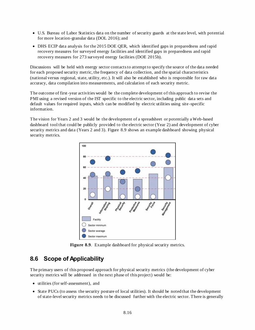
8.16
U.S. Bureau of Labor Statistics data on the number of security guards at the state level, with potential
for more location-granular data (DOL 2016); and
DHS ECIP data analysis for the 2015 DOE QER, which identified gaps in preparedness and rapid
recovery measures for surveyed energy facilities and identified gaps in preparedness and rapid
recovery measures for 273 surveyed energy facilities (DOE 2015b).
Discussions will be held with energy sector contacts to attempt to specify the source of the data needed
for each proposed security metric, the frequency of data collection, and the spatial characteristics
(national versus regional, state, utility, etc.). It will also be established who is responsible for raw data
accuracy, data compilation into measurements, and calculation of each security metric.
The outcome of first -year activities would be the complete development o f this approach to revise the
PMI using a revised version of the IST specific to the electric sector, including public data sets and
default values for required inputs, which can be modified by electric utilities using site -specific
information.
The vision for Years 2 and 3 would be the development of a spreadsheet or potentially a Web-based
dashboard tool that could be publicly provided to the electric sector (Year 2) and development of cyber
security metrics and data (Years 2 and 3). Figure 8.9 shows an example dashboard showing physical
security metrics.
Figure 8.9. Example dashboard for physical security metrics.
8.6 Scope of Applicability
The primary users of this proposed approach for physical security metrics (the development of cyber
security metrics will be addressed in the next phase of this project) would be:
utilities (for self-assessment), and
State PUCs (to assess the security posture of local utilit ies). It should be noted that the development
of state-level security metrics needs to be discussed further with the electric sector. There is generally

8.17
a reluctance by electric utilities to share physical security information because of the inherent nature
of the topic (i.e., making an electric utility more vulnerable to attack by giving out intelligence about
its systems, weaknesses, monitoring methods, etc.). This may limit the potential application of the
proposed approach to develop state-level security metrics scores.
8.6.1 Asset, Distribution, and Bulk Power Level
The PMI approach starts at the asset level and determines the PMI score for key assets such as
substations, control centers, and electric generation facilities.1 The PMI approach was selected for
physical security metrics development because a version of these metrics has been applied by DHS to
over 400 electric assets. The application of the PMI approach would address the lack of consistent
information about the security posture of the electric sector.
The process described in Figure 8.3 will produce a revised PMI, specifically tailored towards electric
sector infrastructure. Electric utilities that have not had DHS personnel conduct an IST survey could
answer a select set of questions that would provide insight into their existing security posture. The revised
set of questions will contain default values that would be determined using statistical analysis of the
available IST data for electric-sector components or publically available data. The utility can then change
those defaults and add additional information specific to their utility to get tailored PMI values for t heir
assets, considering their threat environment.
Recall from the previous section that t he PMI is constituted by five Level 1 components, 25 Level 2
subcomponents, and 64 Level 3 subcomponents. Figure 8.10 provides a typical IST dashboard showing
calculated overall PMI and its five sub-metrics. The proposed approach is to develop a similar PMI
dashboard for electric-sector components that would focus on the five Level 1 components using IST
answers to developed default values and/or public data sets.
1 The NERC CIP-002 standard describes how utilities define critical assets, as well as critical “ cyber” assets.
Essentially, all bulk transmission assets are deemed critical, and utilities may designate additional assets as critical
based on other factors. The first requirement under the CIP 014 standard is for utilities to identify transmission
stations, substations, and control centers that—if rendered inoperable or severely damaged—could result in
widespread instability, uncontrolled separation, or cascading failures within an interconnection.

8.18
Figure 8.10. IST dashboard showing calculated PMI and its five sub-metrics.
For the PMI, the information collected characterizes the weakest protective measures (i.e., the weakest
portion of fence if types and characteristics vary). Some of these values can be inferred from current
industry practice (NERC and similar standards). IST summary information for typical electric-sector
responses, as provided by DHS, indicates that almost all electric substations have performed background
checks, and contain fencing and gates, etc. as shown in Figure 8.11 and Figure 8.12.
Figure 8.11. Typical responses to IST questions for electric substations.

8.19
Figure 8.12. Typical responses to IST questions for electric generation plants.
The PMI requires information that may not be available from public data sources, such as MOUs/MOAs
with local law enforcement and the characteristics of security forces. These gaps in publi cly available data
would be supplemented by analysis previously performed by Argonne to identify gaps in preparedness
and rapid recovery measures for the QER using data collected for 170 electric facilities from January
2011 through September 2014 (DOE 2015d). The electric facilities considered in the previous Argonne
analysis included transmission and distribution substations as well as control rooms and power plants,
which are identified in the NERC CIP 014 standard as key physical assets and may be part of an utility’s
critical facility list (Shumard and Schneider 2014).
It can be expected that the current physical security posture of a given electric utility may depend on
historical crime statistics,
urban vs. suburban vs. rural locations of critical electric assets,
prior incidents of vandalism and sabotage, and
instances of copper theft, etc.
It is well known that substation design differs depending on its location; enclosed substations in urban
areas typically are located within buildings (Figure 8.13), while open-air substations in rural areas are
built without any secondary enclosure (Figure 8.14). The existence of any secondary enclosures such as
buildings is a major physical security benefit that would be reflected in the PMI score for enclosed
substations.

8.20
Figure 8.13. An enclosed substation (note indoor design blends in with its surroundings).
Figure 8.14. An open-air substation (note absence of secondary containment).
The proposed approach will investigate whether PMI scores for electric utilities correlate with historic al
crime statistics, prior incidents of vandalism and sabotage, and other physical security -related issues. The
analysis will be limited to those electric sector facilities for which DHS IST data are readily available
(over 400 electric assets).
8.6.2 Utility Level
Overall PMI for a given electric utility would be the weighted sum of the PMIs for expensive ha rd-to-
replace assets, such as substations, power plants, and control rooms, consistent with the approach in the
NERC CIP 014 Standard for Physical Security . The approach would ignore assets such as transmission
towers, which can be quickly and easily replaced and are assumed to be not as critical as long-lead–t ime
equipment such as transformers in substations, etc.
The overall PMI for an electric utility would account for the PMI scores of its critical assets, which are
assumed to include the utility control center(s), distribution and transmission substations, and electric
generation plants:

8.21
(PMI)utility = ∑ (nj * IFj * PMIj) / ∑ (n j)
where
(PMI)utility = the composite PMI score for the electric utility;
ni = the number of assets of category “i”;
IFi = the importance factor of asset category “i” [an IF of 1 would mean all assets are
equally important];
PMIi = the PMI score for asset category “i”.
Information about the number and characteristics of each utility’s control center(s), distribution and
transmission substations, and electric generation plants would be collected from the following sources:
electric utility control center data based on the location of the electric utility headquarters
electric substation data from Platts Electric Substation geospatial data layer1
electric generation plant data from the EIA-860, Annual Electric Generator Report, EIA-860M,
Monthly Update to the Annual Electric Generator Report and EIA-923, Power Plant Operations
Report.2
8.6.3 State Level
One potential approach to determining the overall PMI for a state would involve the PMI scores for the
electric utilities located within the state, normalized by the number of electric utility customers:
(PMI)state = ∑ { (PMI)utility * ncustomers} / ∑ (ncustomers)
where (PMI)state is the composite PMI score for the electric utility sector in the state, and n customers is the
number of electric customers by utility in the state, as provided by EIA forms EIA-861- schedules 4A &
4D and EIA-861S.3
Other approaches exist for determining the overall PMI for a State based on the PMI for each electric
utility, such as normalizing using
the total capacity of each electric utility, as provided in Form EIA-8264;
the total number of electric assets for each electric utility, as provided by EIA;
the total revenue of each electric utility, as provided by EIA forms EIA-861- schedules 4A & 4D and
EIA-861S;5 and
1 Platts, undated. Electric Substations Metadata – Platts, available at
http://www.platts.com/IM.Platts.Content/ProductsServi ces/Products/gismetadata/substatn.pdf, accessed January 25,
2017. 2 EIA, 2017. “ Layer Information for Interactive State Maps – Power Plants,” available at
http://www.eia.gov/maps/map_data/PowerPlants_US_EIA.zip, accessed January 25, 2017. 3 EIA, 2017. “ 2015 Utility Bundled Retail Sales- Total,” available at
http://www.eia.gov/electricity/sal es_revenue_pri ce/xls/t able10.xlsx, accessed January 25, 2017. 4 EIA (Energy Information Administration). 2017. “ Form EIA-826 detailed data,” available at
http://www.eia.gov/electricity/data/ eia826/, accessed January 25, 2017. s 5 EIA (Energy Information Administration). 2017. “ 2015 Utility Bundled Retail Sales- Total,” available at
http://www.eia.gov/electricity/sal es_revenue_pri ce/xls/t able10.xlsx, accessed January 25, 2017.

8.22
the number of critical sites such as healthcare facilities (hospitals and senior care centers), first
responder (police and fire) stations, mass transit facilities, data centers, and wastewater treatment
plants (WWTPs).1
The most appropriate way to combine individual PMI scores for each electric utility into a composite PMI
score for the electric sector in a state would be determined through consul tation with electric-sector
subject matter experts. Preferences for the specific values for these weights will be determined via a
formal elicitation process and would account for factors such as variations in facility vulnerability
between electric utilit ies. Sensitivity analysis would be performed to determine whether the weights are
reasonable.
8.6.4 Regional Level
The proposed approach to determining the overall PMI at the regional level would involve the PMI scores
for the electric utilities located within t he region, similar to the approach proposed at the state level.
8.6.5 National Level
The proposed approach to determining the overall PMI at the national level would involve the PMI scores
for the electric utilities located within the nation, similar to the appr oach proposed at the state level.
8.6.6 Other Level
The approach at this level is yet to be determined.
8.7 Use-Cases for Metrics
8.7.1 Smart Reconfiguration of Idaho Falls Power Distribution Network for Enhanced Quality of Service
The objective of the GMLC project tit led “Smart Reconfiguration of Idaho Falls Power Distribution
Network for Enhanced Quality of Service” is to identify existing technology and integration
solutions/methods that could be applied to the Idaho Falls utility system, which relies on significant
amounts of imported power to keep as much of the system operating as possible during system events at
both the transmission and distribution levels. Improving physical security at Idaho Falls substations is
something that is specifically called out (although with a focus on reducing the impact of any incidents
via smart system design, e.g., islanding). There may be potential to apply the PMI demo tool under
development to estimate the composite PMI score for the Idaho Falls utility system, to more broadly
understand the current physical security state and how proposed actions might improve it .
The physical security metrics team has contacted the GMLC project lead for the Idaho Falls GMLC
activity to understand how the work being performed compares to what was originally scoped, including
1 FEMA (Federal Emergency Management Agency). 2013. Performance of Critical Facilities and Key Assets,
available at https://www.fema.gov/media-library-dat a/1385587199555-
ebd60a9506168b4fd5a79ee519520c1e/Sandy_MAT_Ch5_508post.pdf, accessed on March 18, 2017.

8.23
physical security, and whether there is interest in examining the physical security opportunity for the
Idaho Falls utility system in greater depth.
8.7.2 Commonwealth Edison
Exploratory discussions are under way with security personn el at Commonwealth Edison (ComEd),
which is the largest electric utility in Illinois and serves the Chicago and Northern Illinois area. ComEd
provides electric service to more than 3.8 million customers across Northern Illinois and its service
territory contains urban, suburban, and rural customers. It also contains transmission (69 to 765 kV),
subtransmission (34.5 kV), and distribution (4.16 to 13.8 kV) substations.
This proposed use-case would provide a spreadsheet or potentially a Web-based dashboard tool that
would contain electric facility data specific to ComEd and estimate the individual Leve l 1 and 2
components for review and comments. Discussions between Argonne and ComEd security personnel are
anticipated and would result in determining the appropriate normalization method and importance factors
specific to substations, control centers, and generating plants. The final outcome would be utility
validation of the PMI approach for the electric sector, including assumptions, data, and default values.
8.8 Value of Metrics
Based on engagements with stakeholders, the following specific values were repo rted:
The DHS IP Assessments Team from the DHS Office of Infrastructure Protection (IP) stated that
DOE’s “grid security metrics efforts” are “examples of opportunities for DHS IP assessments to
contribute to DOE efforts.”
In an initial discussion describing the methodology, NARUC staff indicated that such a comparative
scale could be useful to provide utility commissions with an understanding of the relative physical
security posture of the utilities within their jurisdictions, and the relative impact of p otential
investments designed to improve physical security, without requiring the utilities to share potentially
sensitive data. A follow-up engagement with NARUC’s critical infrastructure resources staff
subcommittee is being planned.
8.9 Feedback from Stakeholders Regarding Year 1 Outcomes
This section summarizes the feedback the research team received from domain experts regarding the
outcome of the Year 1 sustainability metrics definitions, the relevance to the community’s needs, and the
overall value for monitoring progress as the grid evolves.
The following reflections stem from a briefing to domain experts who offered to review the team’s Year 1
results. The reviewers represented DHS, EEI, EPRI, and NASEO. The following is a synopsis of the key
points made during the 1.5 hour briefing:
Technical considerations:
– The aggregation of multiple indicators representing detailed information about the security
posture may not be meaningful because an aggregated indicator masks the higher detailed
information. It was suggested to present both the sub-indicators that make up the PMI as well as
the PMI

8.24
– One reviewer suggested providing as much transparency as possible about the underlying
assumptions of security measures that were considered in the formulation of the approach and
tool development .
Value of work – Reviewers generally saw that the approach could provide value to an electric utility
and regulators and state energy offices in the following respects:
– The metrics approach was viewed as useful for utilit ies to understand better the relative strength
of their physical security posture as well as how they compare against peers.
– The metric approach could be useful for identifying strategies to improve specific physical
security practices within their organization.
– Information derived from the developed approach could be useful for informing rate-recovery
decisions with or without consideration of the peer comparisons.
– General concern was expressed about the appropriateness of using the method for peer
comparison or even presenting geographically aggregated protected measures index values. This
concern in part stemmed from prior experience where some reviewers have seen metrics for other
projects be used to create unfair judgments among and between entities that co uld lead to
inappropriate policies.
– The reviewers also recognized challenges associated with protecting the electric utility -completed
data.

9.1
9.0 Baselining Year 1 Metrics
This section addresses the question of how the proposed metrics that currently do not exist can be
baselined. (Note that this does not apply to the existing metrics, such as GHG emissions). By baselining,
we mean how the metrics can be calculated or measured to assume their first estimation that is considered
a basis or reference, either for the next year’s estimation or to be estimated for a different asset or utility
organization; thus establishing a basis or baseline for the metrics.
One of the main objectives of this effort is to provide a quantitative fram ework for measuring the progress
of grid modernization in various regions of the country. The metric categories were in part selected by
DOE to provide a balanced view of the state of the grid at any point in time, recognizing that tradeoffs
between categories could occur as modernization investments are made. For example, the implementation
of investments that target improved system flexibility could also benefit grid reliability and resilience,
could improve environmental sustainability through supporting increased adoption of variable clean
generation technologies, but might require increased cost to customers in the near -term. Measuring grid
modernization progress can be considered from several different activity perspectives:
The impact of completed Grid Modernization Initiative research, development, demonstration, and
deployment (RD3) program activities on the pace and scale of the modernization of the U.S. grid over
time.
The impact of a specific investment related to a technology demonstration projec t or a production
implementation by a utility, ISO/RTOs, or other market participant, or of a specific legislative or
regulatory policy, or market mechanism, on the specific targeted geographic area in which the project
occurs or the policy or mechanism is meant to affect.
The overall impact of the total portfolio of grid modernization activities, both in terms of the evolving
technology make-up of the grid (including its generation mix) and the policy and regulatory context
that influences both the deployment of technologies on the grid and the constraints under which the
grid can be operated.
In addition, progress for each of these perspectives can be measured from different time considerations:
Prospectively: The future impact of the activity can be estim ated prior to its actual completion or
implementation on the grid. In some cases, these impacts can be expressed as projected costs and
benefits and included in the analysis that informs a decision to proceed with the activities.
Retrospectively: The impact of the activity can be assessed after its actual implementation, either
through application of formal evaluation methods or through ongoing data collection and reporting
efforts.
For any of the activity perspectives, and for either time consideration, de termination of the impact of an
activity is often made by comparing two grid states or scenarios:
The state of the current or expected grid prior to or without the implementation of the activity
The actual or expected state of the grid after or with the im plementation of the activity
The difference between the two states is then a measure of impact of the activity on the grid. The first of
these states is often referred to as a baseline. In the case of a retrospective impact analysis, the baseline
consists of actual measured attributes of then current state of the grid (e.g., historical time series at some
t ime interval). For a prospective analysis, the baseline often takes the form of a “business as usual”
projection, usually modeled, of what might be expected to occur going forward without the activity
occurring.

9.2
This effort is intended to formalize specific metrics in each of the six attribute categories. These
formalized metrics are not meant to represent a complete set of metrics that might be necessary to inform
a broad understanding of impacts within each category (e.g., see Appendix A for an inventory of
potentially useful metrics for each attribute category, most of which are currently reported for at least
some geography within the United States). The metrics being formalized are appropriate for application to
only the latter two act ivity perspectives identified above.1 Depending on the attribute category, the
formalized metrics may be suitable for application to one or both time considerations. As such, the type of
baseline appropriate for each category varies.2
Table 9.1 summarizes the applicable baseline(s) by metric or metrics class for each category, and the
status and potential geographic scope of the documentation of such a baseline. This baseline
characterization is informed significantly by stakeholder feedback on the applicable use of the metrics.
Following the table, a brief context is provided for each of the categories.
1 The attribution of impacts to specific sources of investment, particularly in research, development, and
demonstration, is a challenging exercise typically approached in retrospective evaluation studies. DOE has a rich
experience assessing its RD3 activities in this manner (for more information, see
https://energy.gov/eere/analysis/program -evaluation ). The National Academies has also conducted retrospective
assessments, including for specific DOE energy programs (see https://www.nap.edu/catalog/10165/energy -
research-at-doe-was-it -worth-it -energy-effici ency). This type of application of grid-related metrics falls outside the
scope of this work effort.
2 Those metrics being formulated in this work effort that have prospective application are informing the
development of a Grid Services and Technologies Valuation Framework in GMLC 1.2.4.

9.3
Table 9.1. Ability to baseline Year 1 metrics by metrics area.
Metrics Category
Baseline Feasibility for Metrics Formalized in Year 1
Status/Plans Retrospective Prospective
Reliability
Distribution – yes
Bulk power – yes
Probabilistic transmission
planning – no
Distribution – no
Bulk power – no
Probabilistic transmission
planning – yes, but would
limited to a "business as usual" comparator to a
specific investment
Metrics have not developed fully.
Baseline development will be considered
in Years 2-3, but is likely to be limited
to specific geographic area(s).
Resilience
For direct and indirect
consequence metrics:
Electrical service- no
Critical electrical service -
no
Restoration - no
Monetary - no
Community function - no
Retrospective baseline
development is hampered by
lack of available historical
data, particularly in relating
outage-related data to
specific hazards.
For direct consequence
metrics - yes, but would be
limited to a "business as
usual" comparator to a
specific hazard and type of
infrastructure.
Prospective baseline development is
planned in Years 2-3 for the pilot case
study.
Flexibility
Flexibility demand – yes
Flexibility supply - yes
Flexibility market balance -
yes
Flexibility demand – yes
Flexibility supply - yes
Flexibility market balance -
yes
Prospective baseline
development would be
limited to a "business as
usual" comparator to a
specific investment, policy,
or market mechanism.
While development of a retrospective
baseline is feasible, significant effort is
required to isolate flexibility-related
events from other system or market-
related conditions. Stakeholders have
also indicated that prospective baselines
associated with potential investment
decisions are more valuable.
Retrospective and prospective baseline
development is planned in Years 2-3 for
the pilot case study.

9.4
Table 9.1. (contd)
Metrics Category
Baseline Feasibility for Metrics Formalized in Year 1
Status/Plans Retrospective Prospective
Sustainability CO2 Emissions – yes
CO2 Emissions – yes
A prospective baseline could
be generated for a recognized
national baseline electric
sector projection (e.g., EIA's
Annual Energy Outlook
Reference Case) or as a
"business as usual"
comparator to a specific
investment, policy, or market
mechanism.
Retrospective baselines at the federal
level for the national data products
examined are included in this report.
These baselines do have some gaps or
limitations, mostly notably the lack of
inclusion of generation sources < 1 MW
in capacity. There are no further plans in
Year 2-3 to develop more geographically
granular retrospective baselines
(although this would be straightforward)
or to pilot a prospective baseline for a
specific case study for CO2 emissions.
Year 2-3 effort is proposed to focus on
development of a Water Risk Metric that
assesses water use in the context of its
availability (in space and time). This
metric could have retrospective and
prospective components, including use
case pilot application.
Affordability
For the residential end-use
sector:
Average customer cost
burden – yes
Affordability gap factor –
yes
Affordability gap headcount
– yes
Affordability gap index –
yes
Affordability gap headcount
index – yes
For the residential end-use
sector:
Average customer cost
burden – no
Affordability gap factor – no
Affordability gap headcount
– no
Affordability gap index – no
Affordability gap headcount
index – no
Prospective baseline
development is limited by the
difficulty of meaningfully
projecting household income.
Retrospective baselines at the national
and state level are included in this report
on an annual time step based on public
data sources. County, service territory,
and local examples are also provided for
California and Alaska. The latter
example uses stakeholder supplied
customer cost data. Year 2-3 plans
include a more detailed pilot application
to a utility service area based on utility-
provided customer bill data, and
examination of the applicability to
nonresidential customer classes.
Security
Physical security index
metrics - yes, but only based
on public information and
default values derived from
DHS critical infrastructure
database
Physical security index
metrics - yes, but would be
limited to a "business as
usual" comparator to a
specific investment or policy
Some stakeholders did not consider
retrospective baselines crossing utility
service territories (e.g., at state or
national level) as being useful and
expressed concern over potential mis-
use. Prospective baseline development is
planned in Years 2-3 for the pilot utility
case study.
9.1 Reliability
Two of the three classes of metrics under development (distribution and bulk power system metrics) are
related to historical data and lend themselves to retrospective analysis. As these metrics are still being

9.5
formalized, pilot baselines are expected to be generated for specific geographic regions as a part of Year
2-3 activities.
The third class of metrics, for probabilistic bulk system planning, is by design leading in nature and can
inform prospective decisions on transmission. Simulation-based modeling methods will be employed to
conduct probabilistic contingency analysis involving variable renewable generation to develop these
metrics. Prospective baseline development would involve simulating the contingencies if no change is
made to the transmission system. This “business as usual” baseline would then be compared to a set of
simulations where a proposed change is made to the bulk system. As these metrics are still being
formalized, pilot prospective baselines are expected to be generated for a specific geographic region as a
part of Year 2-3 activities as part of a collaboration with a utility or RTO.
9.2 Resilience
Stakeholders confirm that resilience metrics formalized in this work effort are most effectively applied in
forward-looking (prospective) analysis focused on specific types of hazard events, rather than
retrospectively based on historical data that is available. Retrospective baseline development is hampered
by lack of available historical data, particularly in relating outage-related data to specific types of hazards.
Prospective baseline development would involve modeling the impact of a set of future events if no
change is made to the electric infrastructure of interest. For the consequence metrics of interest, the
baseline is based on a modeled set of simulations that typically estimates the consequences of the set
future events with “business as usual” assumptions. This “business as usual” baseline would then be
compared to a modeled set of simulations where a proposed set of actions or investm ents is made.
9.3 Flexibility
Historical data from CAISO archives can be used to develop a retrospective baseline to assess current
system flexibility for this pilot test area, relying on reports in press related to flexibility. For example,
wind and solar curtailment metrics can be baselined to assess current flexibility of the system. The
challenge is to differentiate between curtailments due to contingencies such as generator or transmission
line forced outages and curtailments due to insufficient ramping capabilities or unit commitment and
dispatch logic that do not position units to provide sufficient flexibility. We plan to work with
stakeholders to identify the frequency and magnitude of these conditions in the historical data and
summarize general trends. Similar baselines for other metrics described in the Reference Document can
also be developed.
Prospective baseline development is also planned for the CAISO pilot, again relying on reports in press
related to flexibility in that region. The prospective baseline would be based on production cost model
outputs for a scenario of “business as usual” assumptions. This “business as usual” baseline would then
be compared to a modeled simulation where a proposed policy, investment, or market mechanism is
implemented.
9.4 Sustainability
Year 1’s effort examined national data products provided by EPA and EIA related to electric sector GHG
emissions. Retrospective baselines at the national level for 6 of the 8 national data products examined are
included in this report for years 2008 - 2014. These baselines do have some gaps or limitations, mostly
notably the lack of inclusion of generation sources < 1 MW in capacity. Two additional data products

9.6
provide forward-looking views of CO2 emissions based on projections of generation mix and associated
fuel consumption and could be considered forms on “business as usual” baselines (not included in this
report). While several recent studies have documented and applied a consistent prospective method, such
prospective application is not included in the scope of this work effort.
For Years 2-3, a Water Risk Metric is proposed to be developed that relates water use by electricity
generation to water availability. This new metric will have prospective and retrospective aspects that
could be developed and applied in a pilot use case.
9.5 Affordability
The formulation of the residential customer cost burden metrics developed in Year 1, and the supporting
customer electricity cost and income data needed to calculate the metrics, lend themselv es to the
development of a retrospective, as opposed to a prospective, baseline. Several examples of such a baseline
for multiple years are included in this report based on publically reported data, including at state and
national levels. Some stakeholders indicated that such a time trend analysis is very useful to assess the
changes over time for a specific utility service territory and felt that this is a more appropriate application
of the formulated metrics than a comparison across geographic areas that could have different energy
consumption patterns.
9.6 Security
It is possible to develop a national retrospective baseline for the physical security index metrics
formalized in this effort based solely on public datasets on the number of electric sector facil ities, which
electric sector facilities have an on-site staff, which utilities have a security force, and others, along with
electric sector-level default values derived from the DHS critical infrastructure database. However, this
baseline may not reflect current electric sector operations due to the reliance on historical data (perhaps
two or more years old). A much-higher confidence level would be achieved through direct involvement
by electric utilities in adjusting the default values and public data to match their current operations.
However, some stakeholders indicated that it could be challenging to recruit electric utilities to update the
physical security metrics and provide the results to a third party for synthesis, given the sensitivity
associated with some of this information.
This utility-specific information could be more forthcoming as a part of a prospective analysis that
compares a “business as usual” baseline to the revised index after a specific security investment within a
utility service territory is made or a policy is implemented.

10.1
10.0 Using Multiple Metrics to Inform Decision-Making
The aforementioned metrics are intended to provide crucial information to stakeholders for enhancing
their decision-making processes with respect to modernization of the electric grid. The categories of
metrics (reliability, affordability, resilience, sustainability, flexibility and security) are the means by
which to measure progress toward modernization . The decision space in which stakeholders operate is
highly complex and requires consideration of multiple, sometimes conflicting, objectives. Understanding
tradeoffs between these objectives is a critical component of assuring the usefulness of the developed
metrics so that they can be used and provide value. Considering tradeoffs between multiple objectives is
further compounded by recognizing the uncertainties associated with each metric .
As part of this overall effort, facilitated discussions with stakeholders will allow metrics team leads to not
only gather input about existing and proposed metrics and their relevance, but also explore how
stakeholders use these metrics and how to they prioritize them to inform decisions. In Year 1, we drew
from stakeholder discussions to propose a structured framework within which stakeholders can weigh
alternative grid technology or policy solutions using multiple metrics. It is the vision for this project that
by Year 3, a structured decision-aiding framework will be developed that enables stakeholders to explore
explicitly several tradeoffs across specific decision spaces using a rich set of grid metrics.

11.1
11.0 References
Argonne (Argonne National Laboratory). 2013. Protective Measures Index and Vulnerability Index:
Indicators of Critical Infrastructure Protection and Vulnerability. Available at
http://www.ipd.anl.gov/anlpubs/2013/11/77931.pdf, accessed June 27, 2016.
Bakshi A, Ahmad K, & Kimar N. 2011. “Security Metrics: Needs and Myths,” International Transactions
in Mathematical Sciences and computers, January-June 2011, Volume 4, No. 1, pp. 31–40 (available at
https://www.researchgate.net/publication/262685082_Security_Metrics_Needs_and_Myths).
Biringer B, Vugrin E, & Warren D. 2013. Critical Infrastructure System Security and Resilience. Boca
Raton: CRC Press.
Brinkman B, Chen C, O’Donnel A, & C Parkes. 2015. Regulation of Physical Security for the Electric
Distribution System . Recommendation document to California Public Utility Commission, February,
2015. Available at https://pdfs.semanticscholar.org/e11b/21010c0fa8e68d0958496bc3564c50524c63.pdf ,
accessed March 21, 2017.
Brotby WK. 2009. “Security Metrics Overview.” Available at
http://www.infosectoday.com/Articles/Security_Metrics_Overview.htm , accessed March 17, 2017.
CAISO (California Independent System Operator). 2014. Flexible Resource Adequacy and Must Offer
Obligation (FRAC MOO) Pre-Market Sim Training. Folsom, California.
CA Legislative Assembly, SB-699 – Public Utilities: Electrical Corporations, 2013-2014. Available at
http://leginfo.legislature.ca.gov/faces/billTextClient.xhtml?bill_id=201320140SB699 , accessed March 21,
2017.
Census. 2016. Table B19001: Household Income in the Past 1 2 Months (In 2015 Inflation-Adjusted
Dollars). Accessed online via Internet Explorer at:
https://factfinder.census.gov/bkmk/table/1.0/en/ACS/15_5YR/B19001/0100000US
Clean Air Act, 42 U.S.C. § 7401 et seq. (1970).
Clean Water Act, 33 U.S.C. § 1251 et seq. (1972).
Cochran J, Miller M, Zinaman O, et al. 2014. Flexibility in 21st Century Power Systems. NREL/TP -
6A20-61721 (2014), National Renewable Energy Laboratory, Golden, Colorado.
Colton RD. 2011. Home Energy Affordability in New York: The Affordability Gap (2008 – 2010).
Prepared for New York State Energy Research Development Authority (NYSERDA) Albany, New York.
Available online at: http://www.nyserda.ny.gov/-/media/Files/EDPPP/LIFE/Resources/2008-2010-
affordability-gap.pdf
CPUC (California Public Utilities Commission). 2015. Beyond 33% Renewables: Grid Integration Policy
for a Low‐Carbon Future: A CPUC Staff White Paper. San Francisco, California.
Denholm P, Novacheck J, Jorgenson J, & O’Connell M. 2016. Impact of Flexibility Options on Grid
Economic Carrying Capacity of Solar and Wind: Three Case Studies. NREL/TP-6A20-66854, National
Renewable Energy Laboratory, Golden, Colorado .

11.2
DHS (Department of Homeland Security). 2009. National Infrastructure Protection Plan, Partnering to
enhance protection and resiliency. Available at https://www.dhs.gov/xlibrary/assets/NIPP_Plan.pdf,
accessed June 27, 2016.
DHS (Department of Homeland Security). 2015. “Critical Infrastructure Vulnerability Assessments.”
Available at https://www.dhs.gov/critical-infrastructure-vulnerability-assessments, accessed June 27,
2016.
DOE (U.S. Department of Energy). 2015a. Grid Modernization Multi-Year Program Plan, November,
2015. Accessed online at: https://energy.gov/downloads/grid-modernization-multi-year-program-plan-
mypp.
DOE (U.S. Department of Energy). 2014. “Cybersecurity Capability Maturity Model (C2M2) Frequently
Asked Questions” Available at https://energy.gov/sites/prod/files/2014/02/f7/C2M2-FAQs.pdf, accessed
March 21, 2017.
DOE (U.S. Department of Energy). 2015b. Quadrennial Energy Review: Energy Transmission, Storage,
And Distribution Infrastructure. Available at
http://energy.gov/sites/prod/files/2015/07/f24/QER%20Full%20Report_TS%26D%20April%202015_0.p
df, accessed June 27, 2016.
DOE (U.S. Department of Energy). 2015c. Quadrennial Energy Review: Energy Transmission, Storage,
and Distribution Infrastructure, “Vulnerabilities of Energy TS&D and Shared Infrastructures to Physical
Attack,” available at
https://energy.gov/sites/prod/files/2015/07/f24/QER%20Full%20Report_TS%26D%20April%202015_0.
pdf, accessed January 26, 2017.
DOE (U.S. Department of Energy). 2015d. Quadrennial Technical Review. Accessed January 23, 2017 at
https://energy.gov/under-secretary-science-and-energy/quadrennial-technology-review-2015
DOE (U.S. Department of Energy). 2016a. “Electricity Subsector Cybersecurity Capability Maturity
Model (ES-C2M2).” Available at http://energy.gov/oe/cybersecurity-capability-maturity-model-c2m2-
program/electricity-subsector-cybersecurity, accessed June 27, 2016.
DOE (U.S. Department of Energy). 2016b. “Electric Disturbance Events (OE-417).” Available at
http://www.oe.netl.doe.gov/oe417.aspx, accessed June 27, 2016.
DOJ (U.S. Department of Justice). 2016. “Uniform Crime Reporting Statistics.” Available at
http://www.ucrdatatool.gov/, accessed June 27, 2016.
DOL (U.S. Department of Labor). 2016. “Occupational Employment and Wages, May 2015, 33 -9032
Security Guards.” Available at http://www.bls.gov/oes/current/oes339032.htm, accessed June 27, 2016.
Drehobl A and Ross L. 2016. Lifting the High Energy Burden in America’s Largest Cities: How Energy
Efficiency Can Improve Low Income and Underserved Communities. American Council for an Energy
Efficient Economy, City, State.
Eaton Corporation plc. 2016. “Blackout and Power Outage Tracker.” Available at
http://powerquality.eaton.com/blackouttracker/default.asp?wtredirect=www.eaton.com/blackouttracker,
accessed June 27, 2016.

11.3
Eberle AL & Heath GA. “CO2 emissions from U.S. electricity may be underestimated as the grid
modernizes.” In preparation for submission to Nature Climate Change. Macmillan Publishers Limited.
EEI (Edison Electric Institute). 2014. Before and After the Storm . Accessed September 30, 2016, at
http://www.eei.org/issuesan dpolicy/electricreliability/mutualassistance/Documents/BeforeandAftertheSto
rm.pdf
EIA (Energy Information Administration). 1996. 1993 Residential Energy Consumption Survey
Microdata. Accessed online at:
https://www.eia.gov/consumption/residential/data/1993/index.php?view=microdata.
EIA (Energy Information Administration). 2004. 2001 Residential Energy Consumption Survey
Microdata. Accessed online at:
https://www.eia.gov/consumption/residential/data/2001/index.php?view=microdata.
EIA (Energy Information Administration). 2009a. 2005 Residential Energy Consumption Survey
Microdata. Accessed online at:
https://www.eia.gov/consumption/residential/data/2005/index.php?view=microdata .
EIA (Energy Information Administration). 2009b. 1997 Residential Energy Consumption Survey
Microdata. Accessed online at:
https://www.eia.gov/consumption/residential/data/1997/index.php?view=microdata .
EIA (Energy Information Administration). 2013. 2009 Residential Energy Consumption Survey
Microdata. Accessed online at:
https://www.eia.gov/consumption/residential/data/2009/index.php?view=microdata .
EIA (Energy Information Administration) 2015. May 15, 2015, EIA’s Today in Energy: “U.S. power
sector CO2 emissions expected to increase through 2040”. Available online at:
https://www.eia.gov/todayinenergy/detail.php?id=21252
EIA (Energy Information Administration). 2016a. “Electric power sales, revenue, and energy efficiency
Form EIA-861 detailed data files,” November 21, 2016. Accessed online at:
http://www.eia.gov/electricity/data/eia861/.
EIA (Energy Information Administration). 2016b. Electric Power Annual. Available at:
http://www.eia.gov/electricity/annual/
EIA (Energy Information Administration). 2016c. Monthly Energy Review. Available at:
http://www.eia.gov/totalenergy/data/monthly/index.cfm
EIA (Energy Information Administration). 2017a. Annual Energy Outlook. Available at:
http://www.eia.gov/outlooks/aeo/.
EIA (Energy Information Administration). 2017b. Short -Term Energy Outlook. Available at:
http://www.eia.gov/outlooks/steo/.
EIA (Energy Information Administration). 2017c. Form EIA-826 detailed data. Available at:
https://www.eia.gov/electricity/data/eia826/.

11.4
Eichman J, Denholm P, Jorgenson J, & Helman U. 2015. Operational Benefits of Meeting California’s
Energy Storage Targets. NREL/TP- 5400-65061, National Renewable Energy Laboratory, Golden,
Colorado. http://www.nrel.gov/docs/fy16osti/65061.pdf
EPA (U.S. Environmental Protection Agency). 2009. Plain English Guide to t he Part 75 Rule. Available
at: https://www.epa.gov/sites/production/files/2015-
05/documents/plain_english_guide_to_the_part_75_rule.pdf .
EPA (U.S. Environmental Protection Agency). 2013. Fact Sheet – Greenhouse Gases Reporting Program
Implementation. Available at: https://www.epa.gov/sites/production/files/2014-
09/documents/ghgfactsheet.pdf.
EPA (U.S. Environmental Protection Agency). 2015a. eGrid. Available at:
https://www.epa.gov/energy/egrid.
EPA (U.S. Environmental Protection Agency). 2015b. GHG Inventory Data Explorer. U.S.
Environmental Protection Agency. Available at:
https://www3.epa.gov/climatechange/ghgemissions/inventoryexplorer/.
EPA (U.S. Environmental Protection Agency). 2016a. Acid Rain Program.
https://www.epa.gov/airmarkets/acid-rain-program
EPA (U.S. Environmental Protection Agency). 2016b. Air Markets Program Data. Available at:
https://ampd.epa.gov/ampd/.
EPA (U.S. Environmental Protection Agency). 2016c. Clean Air Markets – Emission Monitoring.
Available at: https://www.epa.gov/airmarkets/emissions-monitoring.
EPA (U.S. Environmental Protection Agency). 2016d. Cross-State Air Pollution Rule. Available at:
https://www.epa.gov/csapr.
EPA. (U.S. Environmental Protection Agency). 2016e. Greenhouse Gas Reporting Program. Available at:
https://www.epa.gov/ghgreporting.
EPA. (U.S. Environmental Protection Agency). 2016f. News Release on 21st annual GHGI. April 15,
2016. https://www.epa.gov/newsreleases/epa-publishes-21st-annual-us-greenhouse-gas-inventory.
EPA (U.S. Environmental Protection Agency). 2017a. EPA’s Emissions & Generation Resource
Integrated Database (eGRID) webpage. March 2, 2017. https://www.epa.gov/energy/emissions-
generation-resource-integrated-database-egrid
EPA (U.S. Environmental Protection Agency). 2017b. Power Profiler.
https://www.epa.gov/energy/power-profiler
EPAct – Energy Policy Act of 2005. 2005. 42 USC 15801 et seq. Public Law No. 109 -58, as amended
EPRI (Electric Power Research Institute). 2014b. Sustainability Metric Compilation for the Electric
Power Industry: Results of Industry Interviews and Metric Database Development. Report number
3002004255. Available at:
http://www.epri.com/abstracts/Pages/ProductAbstract.aspx?ProductId=000000003002004255 .

11.5
EPRI (Electric Power Research Institute). 2015a. Distribution Grid Resiliency: Prioritization of Options.
EPRI, Palo Alto, CA: 2015. 3002006668.
EPRI (Electric Power Research Institute). 2015b. Sustainability Reporting Trends for the Electric Power
Industry. Report number 3002006996. Available at:
http://www.epri.com/abstracts/Pages/ProductAbstract.aspx?ProductId=000000003002006996 .
EPRI (Electric Power Research Institute). 2016a. “Metrics to Benchmark Sustainability Performance for
the Electric Power Industry.” Report number 3002007228. Available at:
http://www.epri.com/abstracts/Pages/ProductAbstract.aspx?ProductId=3002007228 .
EPRI (Electric Power Research Institute). 2016b. “Power Delivery and Utilization - Distribution and
Utilization, Program 183 - Cyber Security and Privacy,” available at http://www.epri.com/Our-
Portfolio/Pages/Portfolio.aspx?program=072143#tab=1 , accessed June 27, 2016.
EPRI (Electric Power Research Institute). 2016c. “Creating Security Metrics for the Electric Sector,
Version 2,” available at
http://www.epri.com/abstracts/Pages/ProductAbstract.aspx?ProductId=000000003002007886 , accessed
March 17, 2017.
EPSA (U.S. Department of Energy Office of Energy Policy and Systems Analysis). 2017. Quadrennial
Energy Review 1.2 - Environment Baseline Vol. 4: Energy-Water Nexus. Available at:
https://energy.gov/sites/prod/files/2017/01/f34/Environment%20Baseline%20Vol.%204--Energy-
Water%20Nexus.pdf.
FERC (Federal Energy Regulatory Commission). 2016. Common Metrics Report: Performance Metrics
for Regional Transmission Organizations, Independent System Operators, and I ndividual Utilities for the
2010-2014 Reporting Period. Docket No. AD14-15-000. Accessed February 10, 2017 at
https://www.ferc.gov/legal/staff-reports/2016/08-09-common-metrics.pdf
Fisher R & Norman M. 2010. Developing measurement indices to enhance protection and resilience of
critical infrastructures and key resources. Journal of Business Continuity 191–206.
Fisher, Sheehan, and Colton. 2013. “Home Energy Affordability Gap.” Accessed online at:
http://www.homeenergyaffordabilitygap.com/.
Hadley SW, Hill LJ, & Perlack RD. 1993. Report on the Study of Tax and Rate Treatment of Renewable
Energy Projects. ORNL-6772, Oak Ridge National Laboratory, Oak Ridge, Tennessee. Available at:
http://www.ornl.gov/~webworks/cpr/v823/rpt/68456.pdf
Hart R & Liu B. 2015. Methodology for Evaluating Cost-effectiveness of Commercial Energy Code
Changes. PNNL-23923, Rev 1, Pacific Northwest National Laboratory, Richland, Washington. Available
online at: https://www.energycodes.gov/sites/default/files/documents/commercial_methodology.pdf
Heindl P & Schuessler R. 2015. Dynamic properties of energy affordability measures. Energy Policy
86:123–132.
IEA (International Energy Agency). 2011. Harnessing Variable Renewables: A Guide to the Balancing
Challenges. City, State.

11.6
IEA (International Energy Agency). 2014. The Power of Transformation: Wind, Sun and the Economics
of Flexible Power Systems. City, State.
IPCC (Intergovernmental Panel on Climate Change). 2006. “2006 IPCC Guidelines for National
Greenhouse Gas Inventories,” volume 2 (Energy). Chapter 2 (Stationary Combustion). Prepared by the
National Greenhouse Gas Inventories Programme, Eggleston H.S., Buendia L., Miwa K., Ngara T . and
Tanabe K. (eds). Published: IGES, Japan. Available at: http://www.ipcc-
nggip.iges.or.jp/public/2006gl/pdf/2_Volume2/V2_2_Ch2_Stationary_Combustion.pdf
Jaquith A. 2007. Security Metrics: Replacing Fear, Uncertainty and Doubt , Pearson Education, Inc.,
Upper Saddle River, NJ.
Lannoye E, Flynn D, and O'Malley M. 2015. "Transmission, Variable Generation, and Power System
Flexibility." IEEE Transactions on Power Systems 30(1):57–66.
Lannoye E, Flynn D, and O'Malley M. 2012. “Evaluation of Power System Flexibility.” IEEE
Transactions on Power Systems 27(2):922–931.
Lew D, G Brinkman, E Ibanez, A Florita, M Heaney, B-M Hodge, M Hummon, G Stark, J King, SA
Lefton, N Kumar, D Agan, G Jordan, and S Venkataraman. 2013. The Western Wind and Solar
Integration Study Phase 2. NREL Technical Report NREL/TP -5500-55588.
http://www.nrel.gov/docs/fy13osti/55588.pdf
Ma J, et. al. 2013. Evaluating and Planning Flexibility in Sustainable Power Systems. IEEE Transactions
on Sustainable Energy 4(1).
Mills A & Wiser R. 2012. Changes in the Economic Value of Variable Generation at High Penetration
Levels: A Pilot Case Study of California. LBNL-5445E, Ernest Orlando Lawrence Berkeley National
Laboratory Berkeley, California. Accessed May 2, 2014: http://emp.lbl.gov/sites/all/files/lbnl-5445e.pdf
NARUC (National Association of Regulatory Utility Commissioners). 2016. Resilience in Regulated
Utilities. Accessed September 30, 2016, at https://pubs.naruc.org/pub/536F07E4-2354-D714-5153-
7A80198A436D
NASEO (National Association of State Energy Officials). 2014. Infrastructure Protection Gateway,
Rapid Survey Tool. Aavailable at http://www.naseo.org/Data/Sites/1/events/riskworkshop/rapid-survey-
tool_12-17-2014.pdf, accessed June 27, 2016.
NERC (North American Electric Reliability Corporation). 2011. Security Guideline for the Electricity
Sector: Physical Security. Available at
http://www.nerc.com/docs/cip/sgwg/Physical%20Security%20Guideline%202011 -10-
21%20Formatted.pdf, accessed April 25, 2017.
NERC (North American Electric Reliability Corporation). 2015. Bulk Electric System Security Metrics
Working Draft. Available at
http://www.nerc.com/comm/CIPC/Bulk%20Electric%20System%20Security%20Metrics%20Working%2
0G1/BES_Security_Metrics_CIPC_March_2015.pdf, accessed June 27, 2016.
NERC (North American Electric Reliability Corporation). 2016. State of Reliability. Available online at
NERC website.

11.7
NERC (North American Electric Reliability Corporation). NERC Standard TPL-001-01 System
Performance Under Normal Conditions. Available online at NERC website
NERC (North American Electric Reliability Corporation). NERC Standard TPL-004 Transmission System
Planning Performance Requirements. Available online at NERC website
NIST (National Institute of Standards and Technology). 2017. “NVD CVSS Support.” Available at
https://nvd.nist.gov/vuln-metrics/cvss. Accessed on March 29, 2017
Norman MA. 2015. Infrastructure Information Collection Division . Available at
http://www.nrc.gov/docs/ML1532/ML15329A121.pdf, accessed June 27, 2016.
NRC (National Research Council). 2012. Disaster Resilience: A National Imperative. National
Academies Press, Washington, D.C. doi:10.17226/13457.
Obama B. 2013. Presidential Policy Directive 21: Critical Infrastructure Security and Resilience ,
Washington, D.C. (https://www.whitehouse.gov/the-press-office/2013/02/12/presidential-policy-
directive-critical-infrastructure-security-and-resil)
SASB (Sustainability Accounting and Standards Board). 2016. Sustainability Accounting Standard,
Infrastructure Sector: Electric Utilities Sustainability Accounting Standard. Available at:
https://www.sasb.org/standards/do wnload/infrastructure-standards-do wnload/.
Seger KA. 2003. Utility Security, The New Paradigm . PennWell Corporation, Tulsa, Oklahoma.
Short W, Packey DJ, & Holt T . 1995. A Manual for the Economic Evaluation of Energy Efficiency and
Renewable Energy Technologies. NREL/TP-462-5173, National Renewable Energy Laboratory, Golden,
Colorado. Available at: http://www.nrel.gov/docs/legosti/old/5173.pdf
Shumard R & S. Schneider. 2014. “Utility Security: Understanding NERC CIP 014 Requirements and
Their Impact ,” Electric Energy Online, available at
http://www.electricenergyonline.com/show_article.php?mag=100&article=813 , accessed March 18, 2017.
Sullivan P, Cole W, Blair N, Lantz E, Krishnan V, Mai T , Mulcahy D, & Porro G. 2015. 2015 Standard
Scenarios Annual Report: U.S. Electric Sector Scenario Exploration . NREL/TP-6A20-64072, National
Renewable Energy Laboratory, Golden, Colorado. Available at:
http://www.nrel.gov/docs/fy15osti/64072.pdf
Taft J & Becker-Dippmann A. 2014. Grid Architecture. PNNL-24044, Pacific Northwest national
Laboratory, Richland, Washington. Accessed online at:
http://www.pnnl.gov/main/publications/external/technical_reports/PNNL-24044.pdf.
The Climate Registry. 2013. General Reporting Protocol. Available at:
https://www.theclimateregistry.org/tools-resources/reporting-protocols/general-reporting-protocol/.
Vugrin ED, Castillo A, and Silva-Monroy C. 2017. Resilience Metrics for the Electric Power System: A
Performance-Based Approach. SAND2017-1493, Sandia National Laboratories, Albuquerque, New
Mexico.
Watson J-P, Guttromson R, Silva-Monroy C, Jeffers R, Jones K, Ellison J, Rath C, Gearhart J, Jones D,
Corbet T , Hanley C, & Walker LT. 2015. Conceptual Framework for Developing Resilience Metrics for

11.8
the Electricity, Oil, and Gas Sectors in the United State. Tech. Report, SAND2014-18019, Sandia
National Laboratories, Albuquerque, New Mexico. Accessed November 2, 2016 at
http://energy.gov/sites/prod/files/2015/09/f26/EnergyResilienceReport_Final_SAND2014 -18019.pdf
WRI/WBCSD (World Resources Institute and the World Business Council on Sustainable Development).
2004. The Greenhouse Gas Protocol: A Corporate Accounting and Reporting Standard, Revised Edition,
March 2004. Available at: http://www.wri.org/publication/greenhouse-gas-protocol.
Zhao J, Zheng T , & Litvinov E. 2016. "A Unified Framework for Defining and Measuring Flexibility in
Power Systems." IEEE Transactions on Power Systems 31.1:339–347.

Appendix A –
Metrics Inventory

A.1
Appendix A
Metrics Inventory
A.1 Reliability
A.1.1 Data
Categorization Summary Historical Supporting Data - Lagging Metrics
Metric
# Sector
Category (from list)
Electric System
Infra-structure
Component (from list)
Metrics
Name Description Motivation Units
Metric
Type
(from
List)
Metric
Classification (from List)
Metric
Use
(from
List)
Primary
User
(from
List)
Secondary
User
(from List
- if
applicable)
Metrics
Tense
(Lagging/
Leading)
Applic-
able to
Valu-
ation
Project (Yes/No)
Data
Available?
(Yes/No)
Geospatial
Resolution (from list)
Temporal
Frequency
of Data
Reporting (from list)
Citation/
Data
Source
Reference
#
Potential
Issues/
Comments
1 Electricity Reliability Transmission
System
Availability
of
Transmission
NERC collects information to
develop transmission metrics
that analyze outage frequency , duration, causes, and many
other factors related to transmission outages. NERC
will also issue an annual public report showing aggregate
metrics for each NERC region,
and each transmission owner reporting TADS data will be
provided a confidential copy of the same metrics for its
facilities.
Need to achieve better
compliance and create
mechanisms to meet FERC order …
requirements.
Multiple metrics Yes, in an
aggregated
form
National,
Region
Year [REL7] Need to
achieve better
compliance and create
mechanisms to meet FERC
order … requirements.
2 Electricity Reliability Distribution System SARFI System Average RMS
(Variation ) Frequency Index
Focus on sag frequency Avg events per
customer
Area/Region Year [REL9, ]
[REL10]
This is
considered a Power Quality
(PQ) measure - some utilities
separate PQ
from Reliability ;
others consider Reliability to
be a subset of PQ
3 Electricity Reliability Distribution System SIARFI System Instantaneous Average RMS (Variation) Frequency
Index
Component of SARFI Events per customer
Area/Region Year [REL9, ] [REL10]
See SARFI comment
4 Electricity Reliability Distribution System STARFI System Temporary Average RMS (Variation) Frequency
Index
Component of SARFI Avg events per customer
Area/Region Year [REL9, ] [REL10]
See SARFI comment
5 Electricity Reliability Distribution System SMARFI System Momentary Average
RMS (Variation) Frequency Index
Component of SARFI Avg events per
customer
Area/Region Year [REL9, ]
[REL10]
See SARFI
comment
6 Electricity Reliability Distribution
System, Transmission
System
SAIFI System Average Interruption
Frequency Index
Customers
interrupted/customers served
Dimensionless Yes Year [REL11] May be
inconsistently applied from
utility to utility
making comparisons
difficult but not impossible
7 Electricity Reliability Distribution System,
Transmission System
SAIDI System Average Interruption Duration Index
Total customer interruption
duration/customers served
Minutes per customer
Yes Year [REL11] May be inconsistently
applied from utility to utility

A.2
Categorization Summary Historical Supporting Data - Lagging Metrics
Metric
# Sector
Category (from list)
Electric System
Infra-structure
Component (from list)
Metrics
Name Description Motivation Units
Metric
Type
(from
List)
Metric
Classification (from List)
Metric
Use
(from
List)
Primary
User
(from
List)
Secondary
User
(from List
- if
applicable)
Metrics
Tense
(Lagging/
Leading)
Applic-
able to
Valu-
ation
Project (Yes/No)
Data
Available?
(Yes/No)
Geospatial
Resolution (from list)
Temporal
Frequency
of Data
Reporting (from list)
Citation/
Data
Source
Reference
#
Potential
Issues/
Comments
making
comparisons difficult but not
impossible
8 Electricity Reliability Distribution
System, Transmission
System
CAIDI Customer Average Interruption
Duration Index
Sum of customer
interruption durations / total customers
interrupted
Hours per
customer
Year [REL11] Not all utilities
track or report this
9 Electricity Reliability Distribution System,
Transmission
System
CAIFI Customer Average Interruption Frequency Index
Total customers interrupted/total
customers served
Events per unit time per
customer
Year [REL11] Not all utilities track or report
this
10 Electricity Reliability Distribution System,
Transmission System
CTAIDI Customer Total Average Interruption Duration Index
A hybrid of CAIDI except customers with multiple
interruptions are counted only once
Hours per customer
Year [REL11] Not all utilities track or report
this
11 Electricity Reliability Distribution System ASAI Average Service Availability Index
Customer hours service availability / Customer
hours service demands
Dimensionless Year [REL11] Not all utilities track or report
this
12 Electricity Reliability Distribution System MAIFI Monthly Average Interruption Frequency Index
Total customer momentary interruptions /
total customers served
Monthly events per customer
Year [REL11] Not all utilities track or report
this
13 Electricity Reliability Distribution System CEMI Customers Experiencing
Multiple Interruptions
Total customers
experiencing more than n sustained outages / total
customers served
Dimensionless Year [REL11] Not all utilities
track or report this
14 Electricity Reliability Distribution System CEMSMI Customers Experiencing
Multiple Sustained Interruption
and Momentary Interruptions
Similar to CEMSI but
includes momentary and
sustained outages
Dimensionless Year [REL11] Not all utilities
track or report
this
15 Electricity Reliability Distribution System CI Customers Interrupted Customers per unit time period
Year [REL11] Not all utilities track or report
this
16 Electricity Reliability Distribution System CMI Customer Minutes Interrupted Minutes per
customer per
unit time period
Year [REL11] Not all utilities
track or report
this
17 Electricity Reliability Distribution System ASIFI Average sy stem interruption frequency index
Total connected kVA of load interrupted / total
connected kVA served
Dimensionless Year [REL11] Not all utilities track or report
this
18 Electricity Reliability Distribution System ASIDI Average System Interruption
Duration Index
Sum of connected kVA
duration of load
interrupted / total connected kVA served
Hours Year [REL11] Not all utilities
track or report
this
19 Electricity Reliability Distribution System CELID Customers Experiencing Long Interruption Durations
total number of customers that have experienced
more than eight interruptions in a single
reporting year/total
customers served
Dimensionless Year Not all utilities track or report
this
20 Electricity Reliability Distribution System SARI System Average Restoration Index
∑(Circuit outage durations)/∑(circuit
outages); duration greater than 60 seconds; defined
over specified time period
Minutes per outage
Year Not all utilities track or report
this

A.3
Categorization Summary Historical Supporting Data - Lagging Metrics
Metric
# Sector
Category (from list)
Electric System
Infra-structure
Component (from list)
Metrics
Name Description Motivation Units
Metric
Type
(from
List)
Metric
Classification (from List)
Metric
Use
(from
List)
Primary
User
(from
List)
Secondary
User
(from List
- if
applicable)
Metrics
Tense
(Lagging/
Leading)
Applic-
able to
Valu-
ation
Project (Yes/No)
Data
Available?
(Yes/No)
Geospatial
Resolution (from list)
Temporal
Frequency
of Data
Reporting (from list)
Citation/
Data
Source
Reference
#
Potential
Issues/
Comments
21 Electricity Reliability Distribution System COR Correct Operation Rate Number of correct
operations/total number of operations commanded
% Year Not all utilities
track or report this
22 Electricity Reliability Distribution System DELI Devices Experiencing Long
Interruptions
Focus on equipment
rather than customers
Count Year Not all utilities
track or report
this; may refer to either utility
or customer devices
23 Electricity Reliability Distribution System DEMI Devices Experiencing Multiple
Interruptions
Focus on equipment
rather than customers
Count Year Not all utilities
track or report
this; may refer to either utility
or customer devices
24 Electricity Reliability Transmission
System
ACOD Average Circuit Outage
Duration
Transmission outage
metric
Minutes No Year Not all utilities
track or report
this; used to compute TACS
25 Electricity Reliability Transmission System
ACSI Average Circuit Sustained Interruptions
Transmission outage metric
Count/time No Year Not all utilities track or report
this; used to compute TACS
26 Electricity Reliability Transmission System
TACS Transmission Availability Composite Score
Complex function of time-weighted outage,
outage duration, and time
between failure statistics
Dimensionless No Year Computed for transmission
utilities by a
private company
27 Electricity Reliability Transmission
System
FOHMY Forced Outages Per Hundred
Circuit Miles Per Year
Used mainly on
transmission sy stems; can
be circuit or sy stem average
Outages per
hundred miles
per year
No Year Note that some
utilities do not
agree that this is a useful
metric
A.1.2 References
Citation/
Data Source
Ref # Citation/Data Source
REL1 Presidential Policy Directive, 2013
REL2 Summary of Proposed Metrics – QER Technical Workshop on Energy Sector Resilience Metrics (4/29/2014)
REL3 http://www.oe.netl.doe.gov/OE417_annual_summary.aspx
REL4 http://www.sciencedirect. com/sci ence/ arti cle/pii/S0301421514002237#bib26
REL5 CPS1 scores
REL6 GADS, http://www.nerc.com/pa/RAPA/gads/P ages/Reports.aspx
REL7 TADS, http://www.nerc.com/pa/RAPA/tads/Pages/default.aspx
REL8 http://www.nerc.com/pa/RAPA/ri/Pages/ InterconnectionF requencyR esponse. aspx
REL9 IEEE Trans Power Delivery, Vol 13, Jan 1998, pp.254-259
REL10 EPRI Reliability Benchmarking Application Guide For Utility/Customer PQ Indices
REL11 1366-2012 IEEE Guide for Electric Power Distribution Reliability Indices

A.4
REL12 Impact of Low Rotational Inertia on Power System Stability and Operation (Andreas Ulbig, et. al.)
REL13 http://www.nerc.com/pa/RAPA/IR OLSOLExceedance/ ALR3-5_Form.pdf
A.2 Resilience
A.2.1 Data
Categorization Summary Historical Supporting Data - Lagging Metrics
Metric
# Sector
Category
(from list)
Electric System
Infrastructure
Component
(from list) Metrics Name Description Motivation Units
Metric Type
(from List)
Metric
Classification
(from List)
Metric
Use
(from
List)
Primary
User
(from
List)
Secondary User
(from List - if
applicable)
Metrics Tense
(Lagging/
Leading)
Applicable
to
Valuation
Project
(Yes/No)
Data
Available?
(Yes/No)
Geospatial
Resolution
(from list)
Temporal
Frequency of Data
Reporting
(from list)
Citation/Data
Source
Reference #
Potential Issues/
Comments
1 Electricity Resilience Transmission
system,
Distribution
system
Electrical service,
measured with one or
more of the following
units: Cumulative
customer-hours of
outages;
Cumulative customer
energy demand not
served; Average
number (or percentage)
of customers that
experience an outage
during a specified time
period
Quantitative,
Numerical
Outcome Decision
Making,
Learning
Utility,
System
Operators
Communities,
federal/state/local
agency/regulator
Leading
(primarily), but
also lagging;
depends on
particular
analysis and
usage
Yes Yes, in some
cases (e.g.,
OMS have
much outage
data)
Interconnection,
RTO, State, Utility
service area,
Distribution system
footprint, Customer
footprint
TBD: triggers for
calculations could
be change in hazard
conditions, new
investment
planning initiative;
perhaps an annual
review
Note: for leading metric analyses,
consequence data may include
uncertainty, i.e., be characterized as a
probability distribution, histogram,
mean & standard deviation, etc. In
addition to selecting the consequence
categories, it is important to select the
appropriate statistical property (e.g.,
mean, value at risk, maximum,
minimum, etc.) that best fits the
analysis and risk tolerance of the
interested parties.
2 Electricity Resilience Transmission
system,
Distribution
system
Critical Electrical
Service, measured with
one or more of the
following units:
Cumulative critical
customer-hours of
outages;
Critical customer
energy demand not
served;
Average number (or
percentage) of critical
loads that experience
an outage
Quantitative,
Numerical
Outcome Decision
Making,
Learning
Utility,
System
Operators
Communities,
federal/state/local
agency/regulator
Leading
(primarily), but
also lagging;
depends on
particular
analysis and
usage
Yes Yes, in some
cases (e.g.,
OMS have
much outage
data)
Interconnection,
RTO, State, Utility
service area,
Distribution system
footprint, Customer
footprint
TBD: triggers for
calculations could
be change in hazard
conditions, new
investment
planning initiative;
perhaps an annual
review
Resilience Transmission
system,
Distribution
system
Restoration, measured
with one or more of the
following units: time to
recovery, cost of
recovery
Quantitative,
Numerical
Outcome Decision
Making,
Learning
Utility,
System
Operators
Communities,
federal/state/local
agency/regulator
Leading
(primarily), but
also lagging;
depends on
particular
analysis and
usage
Yes Yes, in some
cases
Interconnection,
RTO, State, Utility
service area,
Distribution system
footprint, Customer
footprint
TBD: triggers for
calculations could
be change in hazard
conditions, new
investment
planning initiative;
perhaps an annual
review
Resilience Transmission
system,
Distribution
system
Monetary, measured
with one or more of the
following units: Loss
of utility revenue;
Cost of grid damages;
Cost of recovery;
Avoided outage cost
Quantitative,
Numerical
Outcome Decision
Making,
Learning
Utility,
System
Operators
Communities,
federal/state/local
agency/regulator
Leading
(primarily), but
also lagging;
depends on
particular
analysis and
usage
Yes Yes, in some
cases
Interconnection,
RTO, State, Utility
service area,
Distribution system
footprint, Customer
footprint
TBD: triggers for
calculations could
be change in hazard
conditions, new
investment
planning initiative;
perhaps an annual
review
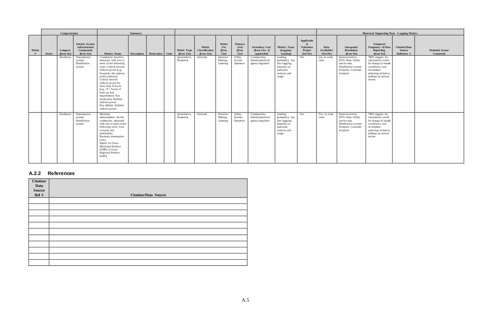
A.5
Categorization Summary Historical Supporting Data - Lagging Metrics
Metric
# Sector
Category
(from list)
Electric System
Infrastructure
Component
(from list) Metrics Name Description Motivation Units
Metric Type
(from List)
Metric
Classification
(from List)
Metric
Use
(from
List)
Primary
User
(from
List)
Secondary User
(from List - if
applicable)
Metrics Tense
(Lagging/
Leading)
Applicable
to
Valuation
Project
(Yes/No)
Data
Available?
(Yes/No)
Geospatial
Resolution
(from list)
Temporal
Frequency of Data
Reporting
(from list)
Citation/Data
Source
Reference #
Potential Issues/
Comments
Resilience Transmission
system,
Distribution
system
Community function,
measured with one or
more of the following
units: Critical services
without power (e.g.,
hospitals, fire stations,
police stations);
Critical services
without power for
more than N hours
(e.g., N > hours of
back up fuel
requirement); Key
production facilities
without power
Key military facilities
without power ;
Quantitative,
Numerical
Outcome Decision
Making,
Learning
Utility,
System
Operators
Communities,
federal/state/local
agency/regulator
Leading
(primarily), but
also lagging;
depends on
particular
analysis and
usage
Yes yes, in some
cases
Interconnection,
RTO, State, Utility
service area,
Distribution system
footprint, Customer
footprint
TBD: triggers for
calculations could
be change in hazard
conditions, new
investment
planning initiative;
perhaps an annual
review
Resilience Transmission
system,
Distribution
system
Monetary
measurements for the
community, measured
with one or more of the
following units: Loss
of assets and
perishables;
Business interruption
costs;
Impact on Gross
Municipal Product
(GMP) or Gross
Regional Product
(GRP);
Quantitative,
Numerical
Outcome Decision
Making,
Learning
Utility,
System
Operators
Communities,
federal/state/local
agency/regulator
Leading
(primarily), but
also lagging;
depends on
particular
analysis and
usage
Yes Yes, in some
cases
Interconnection,
RTO, State, Utility
service area,
Distribution system
footprint, Customer
footprint
TBD: triggers for
calculations could
be change in hazard
conditions, new
investment
planning initiative;
perhaps an annual
review
A.2.2 References
Citation/
Data
Source
Ref # Citation/Data Source

A.6
A.3 Flexibility
A.3.1 Data
Categorization Summary Historical Supporting Data - Lagging Metrics
Metric
# Sector
Category
(from list)
Electric
System
Infrastructure
Component
(from list) Metrics Name Description Motivation Units
Metric
Type (from
List)
Metric
Classification
(from List)
Metric Use
(from List)
Primary User
(from List)
Secondary
User (from List - if
applicable)
Metrics
Tense (Lagging/
Leading)
Applicable
to
Valuation
Project
(Yes/No)
Data
Available?
(Yes/No)
Geospatial
Resolution
(from list)
Temporal
Frequency
of Data
Reporting
(from list)
Citation/
Data
Source
Reference
#
Potential
Issues/
Comments
1 Electricity Flexibility Generation
central
System Regulating
Capability (TVA)
Ratio of the
regulating reserve, demand
response, can quick start
capacity to the
sy stem peak load.
Used to score
portfolios of generating
resources developed using
various strategies
and across various
portfolios. The sy stem regulating
capability measures the
ability of the
portfolio to respond to load
swings.
Normalized Intensity Learning,
Decision-making,
Demonstration
Utility System
operator/planner
Leading [FLEX1] This is a
scoring metric used by TVA in
their 2015 IRP. A lower score
is worse, as it
indicates less capability to
respond to swings.
Strategies that emphasized
renewables had
lower scores, as did strategies
with more energy
efficiency .
They plan to refine it.
2 Electricity Flexibility Generation central
Variable Energy Resource
Penetration (TVA)
Ratio of the variable
resource nameplate
capacity to the
sy stem peak load.
Measures the amount of
variable energy resource included
in a portfolio.
Normalized Intensity Learning, Demonstration
Utility System operator/planner
Leading [FLEX1] This is a reporting
(rather than scoring) metric
used by TVA in
their 2015 IRP. A higher value
indicates more variable
renewables are included in the
portfolio.
3 Electricity Flexibility Generation
central
Flexibility
Turndown Factor
(TVA)
Ratio of the
must run and
non-dispatchable
energy (wind, solar, and
nuclear) to the
annual sales.
Measures the
ability of the
sy stem to serve low load periods.
Normalized Intensity Learning,
Demonstration
Utility System
operator/planner
Leading [FLEX1] This is a
reporting
(rather than scoring) metric
used by TVA in their 2015 IRP.
A higher score
indicates a greater need for
dispatchable plants to be
able to turn down.

A.7
Categorization Summary Historical Supporting Data - Lagging Metrics
Metric
# Sector
Category
(from list)
Electric
System
Infrastructure
Component
(from list) Metrics Name Description Motivation Units
Metric
Type (from
List)
Metric
Classification
(from List)
Metric Use
(from List)
Primary User
(from List)
Secondary
User (from List - if
applicable)
Metrics
Tense (Lagging/
Leading)
Applicable
to
Valuation
Project
(Yes/No)
Data
Available?
(Yes/No)
Geospatial
Resolution
(from list)
Temporal
Frequency
of Data
Reporting
(from list)
Citation/
Data
Source
Reference
#
Potential
Issues/
Comments
4 Electricity Flexibility Generation central
Flexible Resource Indicator (WECC)
Ratio of natural gas-fired
combustion
turbine nameplate
capacity and 15% of
hydropower
capacity to the nameplate
capacity of wind
Provides a general ratio of
the amount of
flexible resources typically used for
balancing VG to the amount of
resource-based
variability in the sy stem. Identifies
circumstances or scenarios where
sufficiency of flexibility might
be a concern and
require more in-depth
examination.
Normalized Intensity Learning, Demonstration
System operator/planner
Leading [FLEX2] WECC used this metric to
highlight
scenarios in the transmission
planning assessment
where
additional studies may be
needed to assess
flexibility .
5 Electricity Flexibility Generation central
Periods of Flexibility Deficit
(EPRI)
Quantity by which potential
demand for flexibility
exceeds the
potential to supply
flexibility (i.e. react to a change
in the net load) for any hour
A post-processing
analy sis that highlights
periods where a
sy stem could be at risk of having
insufficient flexibility if a
rapid change in the net load were
to occur. This
analy sis could be applied to past
observed sy stem dispatch
outcomes or to
simulations of future dispatches.
MW of flexibility
deficit in the up or down
direction for
each hour
Absolute Learning Utility System operator/planner
Lagging or
Leading
[FLEX3] EPRI has a software tool
that can be used to calculate the
flexibility
deficit for any historical
dispatch or using any
production cost model
simulation of
future dispatch. ERCOT
demonstrated the use of the
tool with
historical data (2014) and with
simulations of the future
market.

A.8
Categorization Summary Historical Supporting Data - Lagging Metrics
Metric
# Sector
Category
(from list)
Electric
System
Infrastructure
Component
(from list) Metrics Name Description Motivation Units
Metric
Type (from
List)
Metric
Classification
(from List)
Metric Use
(from List)
Primary User
(from List)
Secondary
User (from List - if
applicable)
Metrics
Tense (Lagging/
Leading)
Applicable
to
Valuation
Project
(Yes/No)
Data
Available?
(Yes/No)
Geospatial
Resolution
(from list)
Temporal
Frequency
of Data
Reporting
(from list)
Citation/
Data
Source
Reference
#
Potential
Issues/
Comments
6 Electricity Flexibility Generation central
Insufficient Ramping Resource
Expectation
The expected number of
observations
when a power sy stem cannot
cope with the changes in net
load, predicted
or unpredicted.
This flexibility metric measures,
in a probabilistic
manner, the ability of a
sy stem to use its resources to meet
both predicted
and unpredicted net load changes,
accounting for how the sy stem
is operated (including
dispatch and
reserves)
Number of observations
with
insufficient ramping
Absolute Learning System operator/planner
Utility Leading [FLEX4] E. Lannoye developed this
metric in an
IEEE paper, it similar to the
EPRI approach albeit more
probabilistic.
7 Electricity Flexibility Generation central
Flexibility Metric (ISO-NE)
Comparison of the largest
variation range (i.e., the
flexibility
supply ) with the target range (the
flexibility demand) to
reflect excessive
availability of the sy stem
relative to the target variation
range.
They use the metric to create a
real-time situation-
awareness tool
for ISO New England that
shows the degree to which
flexibility
capability exceeds the
flexibility need in operational
settings looking out over the next
few hours.
Where flexibility is limited, the
operators can use the information
to identify
corrective actions while many
options are still available.
Binary (is there a
shortage or not?)
Absolute Learning, Decision
Making
System operator/planner
Utility Leading [FLEX5] This is a very rigorous
definition of flexibility that
accounts for the
transmission network.

A.9
Categorization Summary Historical Supporting Data - Lagging Metrics
Metric
# Sector
Category
(from list)
Electric
System
Infrastructure
Component
(from list) Metrics Name Description Motivation Units
Metric
Type (from
List)
Metric
Classification
(from List)
Metric Use
(from List)
Primary User
(from List)
Secondary
User (from List - if
applicable)
Metrics
Tense (Lagging/
Leading)
Applicable
to
Valuation
Project
(Yes/No)
Data
Available?
(Yes/No)
Geospatial
Resolution
(from list)
Temporal
Frequency
of Data
Reporting
(from list)
Citation/
Data
Source
Reference
#
Potential
Issues/
Comments
8 Electricity Flexibility Generation central
System Flexibility (PSE)
Comparison of the flexibility
supply from
generating resources
(primarily the utilities share of
hydroelectric
generating facilities, but
also the of simple- and
combined-cycle gas-fired units)
to the flexibility
demand (based on the volatility
observed in load, generation
and transmission
curtailments, and the
uncertainty inherent in
predicting loads, wind generation
and unexpected
events).
Process to evaluate the
flexibility of a
utilities planned system in an
integrated resource plan.
Average MW of
unmet
reserves in hour-ahead
balancing and unmet
reserves in
intra-hour balancing
Absolute Learning, Decision
Making
Utility Leading [FLEX6] PSE use this analy sis to
evaluate their
portfolio of resources. They
also included an analy sis on
the impact of
adding additional
flexible generation on
reducing the balancing costs,
highlighting the
economic implications of
flexibility .
9 Electricity Flexibility Generation central
Net Demand Ramping
Variability (NERC ERSTF)
Historical and projected
maximum one-hour-up, one-
hour-down,
three- hour-up, and three-hour-
down net demand ramps
(actual load less
production from VERs) using
one-minute data.
Measures the maximum net
demand variability faced
by a balancing
authority . Ultimately , the
BA needs to have adequate
resources
available to meet the expected
demand variability .
Tracking this metric allows for
early
identification of potential areas
for further analy sis.
MW of net demand
variability
Absolute Learning System operator/planner
Utility Lagging or
Leading
[FLEX7] This is Measure 6 of the most
important essential
reliability
services identified by
NERC's Essential
Reliability
Services Task Force.

A.10
Categorization Summary Historical Supporting Data - Lagging Metrics
Metric
# Sector
Category
(from list)
Electric
System
Infrastructure
Component
(from list) Metrics Name Description Motivation Units
Metric
Type (from
List)
Metric
Classification
(from List)
Metric Use
(from List)
Primary User
(from List)
Secondary
User (from List - if
applicable)
Metrics
Tense (Lagging/
Leading)
Applicable
to
Valuation
Project
(Yes/No)
Data
Available?
(Yes/No)
Geospatial
Resolution
(from list)
Temporal
Frequency
of Data
Reporting
(from list)
Citation/
Data
Source
Reference
#
Potential
Issues/
Comments
10 Electricity Flexibility Generation central
LOLE_flex (LOLE multi_hour
and
LOLE_intra_hour)
Attributes loss of load events
during times
when generation capacity was not
limited (i.e. there was excess
capacity
available, but it could not be
accessed due to flexibility
constraints) to either multi-hour
or intra-hour
flexibility deficits.
Expand the traditional
definition of
LOLE to account for operating
flexibility in order to answer
the question of:
How much capacity and
operating flexibility is
needed for a power sy stem to
meet the 1 day in
10 years Loss of Load Expectation
(LOLE) reliability
standard?
Days with Loss of Load
in 10 Years
Absolute Learning, Decision
Making
System operator/planner
Utility Leading [FLEX8] This expanded definition of
LOLE was
developed in the CES-21
project and implemented in
a commercial
production cost model called
SERVM by ASTRAPE
consulting.
11 Electricity Flexibility Generation central
Binding flexibility ratio
Measures the ratio of the
flexibility
demand to the flexibility
supply in the operational time
interval where
flexibility is most binding.
In order to better gauge the
flexibility of
planned resource portfolios, we
developed a way to measure, at a
screening-level,
the overall flexibility of a
portfolio.
Normalized Intensity Learning Utility State Regulator Leading [FLEX9] This is a screening-level
metric that was
applied to resource
portfolios included in the
Resource
Planning Portal, a database of
IRPs from utilities in the
Western U.S.
12 Electricity Flexibility Generation
central
Flexible Capacity
Need (CAISO)
A monthly
measure of the maximum 3-
hour contiguous ramp in the net
load plus the larger of the
most severe
single contingency or
3.5% of the monthly peak
load.
Part of an annual
flexible capacity technical study to
determine the flexible capacity
needed to help ensure the
sy stem
reliability . The flexible capacity
need is then allocated to
LSEs.
MW of
flexible capacity
Absolute Decision
Making, Accountability
System
operator/planner
State Regulator Leading [FLEX10] The CAISO
calculates the flexible
capacity need on an annual
basis for the CPUC and for
its Flexible
Resource Must Offer
Obligation.
13 Electricity Flexibility Generation
central
Renewable
Curtailment
Percentage of
the available renewable
energy that must
be curtailed due to flexibility
limitations.
Highlight the
consequences of insufficient
flexibility
Normalized Absolute Learning,
Decision Making
System
operator/planner
State Regulator Lagging
or Leading
[FLEX11] Numerous
studies have focused on
curtailment of
RE as a sign of inflexibility .
E3's study is a particularly
good example.

A.11
Categorization Summary Historical Supporting Data - Lagging Metrics
Metric
# Sector
Category
(from list)
Electric
System
Infrastructure
Component
(from list) Metrics Name Description Motivation Units
Metric
Type (from
List)
Metric
Classification
(from List)
Metric Use
(from List)
Primary User
(from List)
Secondary
User (from List - if
applicable)
Metrics
Tense (Lagging/
Leading)
Applicable
to
Valuation
Project
(Yes/No)
Data
Available?
(Yes/No)
Geospatial
Resolution
(from list)
Temporal
Frequency
of Data
Reporting
(from list)
Citation/
Data
Source
Reference
#
Potential
Issues/
Comments
14 Electricity Flexibility Generation central (RTO,
ISOs)
Percent of unit-hours mitigated
Percentage of unit hours that
prices were set
at the mitigated price on an
annual basis.
High values of this metric may
be due to a lack
of flexibility in the sy stem.
CAISO reported the highest
percentage of
mitigated hours in this report.
CAISO has large intermittent
renewable fleet requiring
flexibility
operations.
Normalized Absolute Learning, Decision
Making
System operator/planner
State Regulator Lagging or
Leading
FERC Common
Metrics
Report
Price mitigation may be due to
component
outages or other factors not
related to flexibility .
Research is
needed to de-convolve these
factors.
15 Electricity Flexibility Generation central (RTO,
ISOs)
Demand response (DR)
DR as a % of total installed
capacity
Provides an indication of the
contribution of
DR to maintaining the
short and long term reliability .
Normalized Absolute Learning, Decision
Making
System operator/planner
State Regulator Lagging or
Leading
FERC Common
Metrics
Report
DR usage, rather than
installed
capacity , would be another
useful metric.
16 Electricity Flexibility Generation
central (RTO,
ISOs)
Control
Performance
Standards (CPS1, CPS2, BAAL)
Control
performance
standards measure a
balancing area's Area Control
Error (ACE),
which indicates how well the
sy stem operators maintain a
balance between supply and
demand. BAs
need to meet NERC-
mandated performance
standards to
show that they are maintaining
an adequate balance.
Decreases in
control
performance indicate that the
sy stem operator is not
maintaining a
balance between supply and
demand. This can be due, in part, to
insufficient flexibility .
Normalized Absolute Accountability System
operator/planner
Federal
Regulator
(FERC/NERC)
Lagging Yes RTO/Balancing
Authority
Monthly NERC
Standards
Poor
performance
could be due to other factors
besides lack of flexibility .

A.12
A.3.2 References
Citation/
Data
Source
Ref # Citation/Data Source
FLEX1 TVA (Tennessee Valley Authority). 2015. “ Integrated Resource Plan - 2015 Final Report.” Knoxville, TN: Tennessee Valley Authority.
http://www.tva.com/environment/reports/irp/pdf/2015_irp.pdf.
FLEX2 WECC (Western Electricity Coordinating Council). 2013. 2013 Interconnection-wide Plan: Plan Summary. Salt Lake City: WECC.
https://www.wecc.biz/Reliability/2013Plan_PlanSummary.pdf.
FLEX3 Electric Power Research Institute (EPRI). 2014. “ Metrics for Quantifying Flexibility in Power System Planning.” Palo Alto, CA : Electric
Power Research Institute. http://www.epri.com/abstracts/P ages/ProductAbstract.aspx?ProductId=000000003002004243.
FLEX4 Lannoye, E., D. Flynn, and M. O’Malley. 2012. “ Evaluation of Power System Flexibility.” IEEE Transactions on Power Systems 27 (2):
922–31. doi:10.1109/TPWRS.2011.2177280.
FLEX5 Zhao, J., T. Zheng, and E. Litvinov. 2015. “ A Unified Framework for Defining and Measuring Flexibility in Power System.” IEEE
Transactions on Power Systems PP (99): 1–9. doi:10.1109/TPWRS.2015.2390038.
FLEX6 Puget Sound Energy. 2015. “ 2015 Integrated Resource Plan: Appendix H - Operational Flexibility.”
http://pse.com/aboutpse/EnergySupply/Pages/Resource-Planning.aspx.
FLEX7
North American Electric Reliability Corporation (NERC). 2015. “ Essential Reliability Services Task Force Measures Framework
Report.” Atlanta, GA: North American Electric Reliability Corporation.
http://www.nerc.com/comm/Other/essntlrlbltys rvcstskfrcDL/ERSTF%20F ramework%20R eport%20-%20Final.pdf.
FLEX8 Flexibility Metrics and Standards Project – a California Energy Systems for the 21st Century (CES-21) Project:
http://www.cpuc.ca.gov/WorkArea/DownloadAsset.aspx?id=9282
FLEX9 Mills, Andrew, and Joachim Seel. 2015. “ Flexibility Inventory for Western Resource Planners.” LBNL-1003750. Berkeley, CA:
Lawrence Berkeley National Laboratory. https://emp.lbl.gov/sites/all/files/lbnl-1003750_0.pdf.
FLEX10 CAISO. Final Flexible Capacity Needs Assessment for 2017.
https://www.caiso.com/Documents/FinalFlexibl eCapacityNeedsAssessmentFor2017.pdf
FLEX11
Energy and Environmental Economics, Inc. 2015. “ Western Interconnection Flexibility Assessment.” San Francisco, CA.
https://www.wecc.biz/_layouts/15/WopiF rame.aspx?sourcedoc=/R eliability/WECC_Flexibility_Assessment_ExecSumm_2016 -01-
11.pdf.
A.4 Sustainability
A.4.1 Data
Categorization Summary Historical Supporting Data - Lagging Metrics
Metric
# Sector
Category
(from list)
Electric
System
Infrastructure
Component
(from list)
Metrics
Name Description Motivation Units
Metric
Type
(from List)
Metric
Classification
(from List)
Metric Use
(from List)
Primary
User
(from List)
Secondary
User (from List
- if
applicable)
Metrics
Tense
(Lagging/
Leading)
Applicable
to
Valuation
Project
(Yes/No)
Data
Available?
(Yes/No)
Geospatial
Resolution
(from list)
Temporal
Frequency
of Data
Reporting
(from list)
Citation/Data
Source
Reference #
Potential
Issues/
Comments

A.13
Categorization Summary Historical Supporting Data - Lagging Metrics
Metric
# Sector
Category
(from list)
Electric
System
Infrastructure
Component
(from list)
Metrics
Name Description Motivation Units
Metric
Type
(from List)
Metric
Classification
(from List)
Metric Use
(from List)
Primary
User
(from List)
Secondary
User
(from List
- if
applicable)
Metrics
Tense (Lagging/
Leading)
Applicable
to
Valuation
Project
(Yes/No)
Data
Available?
(Yes/No)
Geospatial
Resolution
(from list)
Temporal
Frequency
of Data
Reporting
(from list)
Citation/Data
Source
Reference #
Potential
Issues/
Comments
1 Electricity Sustainability Generation central
Electric sector CO2
emissions
from GHGRP
Absolute CO2
emissions as
reported to the GHGRP
under mandatory
facility
reporting to EPA
Mandatory reporting
under EPA's
Greenhouse Gas
Reporting Program
(CFR 40 Part
98); facilities that emit
25,000 metric tons or more
per year of GHGs are
required to
submit annual reports to
EPA under the GHGRP
Metric tons of
CO2
equivalents
Absolute Outcome Learning, Decision-
making,
Accountability , Demonstration
EPA Utility Lagging Yes Yes Generation plant
Annually SUS1
2 Electricity Sustainability Generation
central
Electric
sector
GHG emissions
from GHGI
Absolute
GHG
emissions as estimated by
the EPA's Greenhouse
Gas Inventory
(GHGI), an
annual top-down
assessment of total US
GHG
emissions and removals
by source and
economic sector
For
submission to
the United Nations in
accordance with the
Framework Convention
on Climate
Change
Metric
tons of
CO2 equivalents
Absolute Outcome Learning,
Decision-
making, Accountability ,
Demonstration
United
Nations
Policy
makers
Lagging No Yes National Annually SUS2
3 Electricity Sustainability Generation central
Electric sector
GHG emissions
from eGRID
Absolute GHG
emissions as compiled by
the EPA into its eGRID
data product;
data sources include
Clean Air Markets
program
(CAMD) and the EIA's
Monthly Energy
Review (MER)
For consumers,
researchers, and other
stakeholders to develop
GHG
inventories, carbon
footprints, consumer
information
disclosure, avoided
emission estimates, etc.
Pounds of CO2;
Pounds of N2O;
Pounds of CH4;
Pounds of
CO2 equivalents
Absolute Outcome Learning, Decision-
making, Accountability ,
Demonstration
Consumers Utility Lagging Yes Yes Boiler Biennially SUS3

A.14
Categorization Summary Historical Supporting Data - Lagging Metrics
Metric
# Sector
Category
(from list)
Electric
System
Infrastructure
Component
(from list)
Metrics
Name Description Motivation Units
Metric
Type
(from List)
Metric
Classification
(from List)
Metric Use
(from List)
Primary
User
(from List)
Secondary
User
(from List
- if
applicable)
Metrics
Tense (Lagging/
Leading)
Applicable
to
Valuation
Project
(Yes/No)
Data
Available?
(Yes/No)
Geospatial
Resolution
(from list)
Temporal
Frequency
of Data
Reporting
(from list)
Citation/Data
Source
Reference #
Potential
Issues/
Comments
4 Electricity Sustainability Generation central
Electric sector
GHG
intensity from
eGRID
GHG intensity as
estimated in
the EPA's eGRID data
product; data sources
include
Clean Air Markets
program (CAMD) and
the EIA's Monthly
Energy
Review (MER)
For consumers,
researchers,
and other stakeholders
to develop GHG
inventories,
carbon footprints,
consumer information
disclosure, avoided
emission
estimates, etc.
Pounds of CO2 per
MWh;
Pounds of N20 per
MWh; Pounds of
CH4 per
MWh; Pounds of
CO2 equivalents
per MWh
Intensity Outcome Learning, Decision-
making,
Accountability , Demonstration
Consumers Utility Lagging Yes Yes Generation plant
Biennially SUS3
5 Electricity Sustainability Generation
central
Electric
sector CO2
emissions from
CAMD
Absolute
CO2
emissions as reported to
the EPA Clean Air
Markets Division
(CAMD) for
mandatory reporting of
CO2 emissions
data from
continuous emission
monitoring sy stems
Mandatory
reporting
under EPA's Acid Rain
Program (CFR 40 Part
75)
Metric
tons of
CO2
Absolute Outcome Learning,
Decision-
making, Accountability ,
Demonstration
EPA Utility Lagging Yes Yes Boiler Hourly SUS4
6 Electricity Sustainability Generation central
Electric sector CO2
emissions
from MER
Absolute CO2
emissions as
compiled by the EIA in its
Monthly Energy
Review (MER)
To provide independent
and impartial
energy information to
promote sound
policymaking, efficient
markets, and
public understanding
Metric tons of
CO2
Absolute Outcome Learning, Decision-
making,
Accountability , Demonstration
Consumers Policy makers
Lagging Yes Yes State Monthly SUS5
7 Electricity Sustainability Generation
central
Electric
sector CO2 emissions
from EIA's
EPA
Absolute
CO2 emissions as
compiled by
the EIA in its Electric
Power Annual
(EPA)
To provide
independent and impartial
energy
information to promote
sound policymaking,
efficient
markets, and public
understanding
Metric
tons of CO2
Absolute Outcome Learning,
Decision-making,
Accountability ,
Demonstration
Consumers Policy
makers
Lagging Yes Yes Facility Annually SUS6

A.15
Categorization Summary Historical Supporting Data - Lagging Metrics
Metric
# Sector
Category
(from list)
Electric
System
Infrastructure
Component
(from list)
Metrics
Name Description Motivation Units
Metric
Type
(from List)
Metric
Classification
(from List)
Metric Use
(from List)
Primary
User
(from List)
Secondary
User
(from List
- if
applicable)
Metrics
Tense (Lagging/
Leading)
Applicable
to
Valuation
Project
(Yes/No)
Data
Available?
(Yes/No)
Geospatial
Resolution
(from list)
Temporal
Frequency
of Data
Reporting
(from list)
Citation/Data
Source
Reference #
Potential
Issues/
Comments
8 Electricity Sustainability Generation central
Electric sector CO2
emissions
from EIA's STEO
Absolute CO2
emissions as
projected by the EIA in its
Short-Term Energy
Outlook
To provide independent
and impartial
energy information to
promote sound
policymaking,
efficient markets, and
public understanding
Metric tons of
CO2
Absolute Outcome Learning, Decision-
making,
Accountability , Demonstration
Consumers Policy makers
Leading No Yes National Monthly SUS7
9 Electricity Sustainability Generation
central
Electric
sector CO2
emissions from EIA's
AEO
Absolute
CO2
emissions as compiled by
the EIA in its Annual
Energy Outlook
To provide
independent
and impartial energy
information to promote
sound policymaking,
efficient
markets, and public
understanding
Metric
tons of
CO2
Absolute Outcome Learning,
Decision-
making, Accountability ,
Demonstration
Consumers Policy
makers
Leading Yes Yes National Annually SUS8
11 Electricity Sustainability Generation,
transmission, and
distribution
Corporate
CO2 emissions
from
SASB
Absolute
GHG emissions
(gross global
scope 1) as reported to
the Sustainability
Accounting
Standards Board
To develop
and disseminate
sustainability
accounting standards that
help public corporations
disclose
material, decision-
useful information to
investors
Metric
tons of CO2
equivalents
Absolute Outcome Learning,
Decision-making,
Accountability ,
Demonstration
Utility Consumer Lagging No Varies Corporation Varies SUS9
12 Electricity Sustainability Generation, transmission,
and
distribution
GHG emissions
covered
under emissions-
limiting regulations
Percentage of emissions
covered
under emissions-
limiting regulations
To develop and
disseminate
sustainability accounting
standards that help public
corporations
disclose material,
decision-useful
information to investors
Percentage Quantitative Process Learning, Decision-
making,
Accountability , Demonstration
Utility Consumer Lagging No Varies Corporation Varies SUS9

A.16
Categorization Summary Historical Supporting Data - Lagging Metrics
Metric
# Sector
Category
(from list)
Electric
System
Infrastructure
Component
(from list)
Metrics
Name Description Motivation Units
Metric
Type
(from List)
Metric
Classification
(from List)
Metric Use
(from List)
Primary
User
(from List)
Secondary
User
(from List
- if
applicable)
Metrics
Tense (Lagging/
Leading)
Applicable
to
Valuation
Project
(Yes/No)
Data
Available?
(Yes/No)
Geospatial
Resolution
(from list)
Temporal
Frequency
of Data
Reporting
(from list)
Citation/Data
Source
Reference #
Potential
Issues/
Comments
12 Electricity Sustainability Generation, transmission,
and
distribution
GHG emissions
covered
under emissions-
reporting regulations
Percentage of emissions
covered
under emissions-
reporting regulations
To develop and
disseminate
sustainability accounting
standards that help public
corporations
disclose material,
decision-useful
information to investors
Percentage Quantitative Process Learning, Decision-
making,
Accountability , Demonstration
Utility Consumer Lagging No Varies Corporation Varies SUS9
12 Electricity Sustainability Generation,
transmission,
and distribution
Corporate
emission
reduction strategy
Description
of long-term
and short-term strategy
or plan to manage
Scope 1
emissions, emission-
reduction targets, and
an analy sis of performance
against those
targets
To develop
and
disseminate sustainability
accounting standards that
help public
corporations disclose
material, decision-
useful information to
investors
NA Qualitative Process Learning,
Decision-
making, Accountability ,
Demonstration
Utility Consumer Leading No Varies Corporation Varies SUS9
12 Electricity Sustainability Generation,
transmission,
and distribution
Corporate
fulfillment
of RPS target by
market
Percentage
fulfillment of
RPS target by market
To develop
and
disseminate sustainability
accounting standards that
help public corporations
disclose
material, decision-
useful information to
investors
Percentage Quantitative Process Learning,
Decision-
making, Accountability ,
Demonstration
Utility Consumer Lagging No Varies Corporation Varies SUS9
12 Electricity Sustainability Generation, transmission,
and distribution
Customers served in
RPS markets
Number of customers
served in markets
subject to
renewable portfolio
standards
To develop and
disseminate sustainability
accounting
standards that help public
corporations disclose
material,
decision-useful
information to investors
Number of customers
Absolute Process Learning, Decision-
making, Accountability ,
Demonstration
Utility Consumer Lagging No Varies Corporation Varies SUS9

A.17
Categorization Summary Historical Supporting Data - Lagging Metrics
Metric
# Sector
Category
(from list)
Electric
System
Infrastructure
Component
(from list)
Metrics
Name Description Motivation Units
Metric
Type
(from List)
Metric
Classification
(from List)
Metric Use
(from List)
Primary
User
(from List)
Secondary
User
(from List
- if
applicable)
Metrics
Tense (Lagging/
Leading)
Applicable
to
Valuation
Project
(Yes/No)
Data
Available?
(Yes/No)
Geospatial
Resolution
(from list)
Temporal
Frequency
of Data
Reporting
(from list)
Citation/Data
Source
Reference #
Potential
Issues/
Comments
13 Electricity Sustainability Generation central
Electric sector CO2
intensity
from EIA
GHG intensity
used to
compute CO2 emissions
from fuel consumption
in the EIA's
Monthly Energy
Review (MER) and
the EIA's Electric
Power
Annual (EPA)
To provide independent
and impartial
energy information to
promote sound
policymaking,
efficient markets, and
public understanding
Million metric tons
of CO2 per
quadrillion Btu
Intensity Outcome Learning, Decision-
making,
Accountability , Demonstration
EIA Lagging No Yes National Not recently
updated
SUS10
14 Electricity Sustainability Generation
central
Electric
sector CO2 intensity
from the
EPA's GHGRP
GHG
intensity reported in
the Code of
Federal Regulations
for use in the Greenhouse
Gas
Reporting Program
(GHGRP)
Mandatory
reporting under EPA's
Greenhouse
Gas Reporting
Program (CFR 40 Part
98); facilities
that emit 25,000 metric
tons or more per year of
GHGs are required to
submit annual
reports to EPA under
the GHGRP
Kilograms
CO2 per million
Btu
Intensity Outcome Learning,
Decision-making,
Accountability ,
Demonstration
EPA Lagging No Yes National One-time
release
SUS11
15 Electricity Sustainability Generation
central
Electric
sector SO2 and NOx
emissions from
eGRID
Absolute
NOx and SO2 emissions as
compiled by the EPA into
its eGRID
data product; data sources
include Clean Air
Markets
program (CAMD) and
the EIA's Monthly
Energy Review
(MER)
For
consumers, researchers
and other stakeholders
to develop
criteria pollutant
emission inventories,
air quality
analy sis, consumer
information disclosure,
avoided emission
estimates, etc.
Tons of
NOx and SO2
Absolute Outcome Learning,
Decision-making,
Accountability , Demonstration
Consumers Utility Lagging Yes Yes Boiler Biennially SUS3

A.18
Categorization Summary Historical Supporting Data - Lagging Metrics
Metric
# Sector
Category
(from list)
Electric
System
Infrastructure
Component
(from list)
Metrics
Name Description Motivation Units
Metric
Type
(from List)
Metric
Classification
(from List)
Metric Use
(from List)
Primary
User
(from List)
Secondary
User
(from List
- if
applicable)
Metrics
Tense (Lagging/
Leading)
Applicable
to
Valuation
Project
(Yes/No)
Data
Available?
(Yes/No)
Geospatial
Resolution
(from list)
Temporal
Frequency
of Data
Reporting
(from list)
Citation/Data
Source
Reference #
Potential
Issues/
Comments
15 Electricity Sustainability Generation central
Electric sector SO2
and NOx
emissions from
eGRID
Absolute NOx and SO2
emissions as
compiled by the EPA into
its eGRID data product;
data sources
include Clean Air
Markets program
(CAMD) and the EIA's
Monthly
Energy Review
(MER)
For consumers,
researchers
and other stakeholders
to develop criteria
pollutant
emission inventories,
air quality analy sis,
consumer information
disclosure,
avoided emission
estimates, etc.
lb NOx and SO2
per MWh.
intensity Outcome Learning, Decision-
making,
Accountability , Demonstration
Consumers Utility Lagging Yes Yes Generation plant
Biennially SUS3
16 Electricity Sustainability Generation central
Electric sector SO2
and NOx
emissions from
CAMD
Absolute SO2 and
NOx
emissions as reported to
the EPA Clean Air
Markets
Division (CAMD) for
mandatory reporting
from continuous
emission
monitoring sy stems
Mandatory reporting
under EPA's
Acid Rain Program
(CFR 40 Part 75)
lb of SO2 and NOx
Absolute Outcome Learning, Decision-
making,
Accountability , Demonstration
EPA Utility Lagging Yes Yes Boiler Hourly SUS4
16 Electricity Sustainability Generation central
Electric sector SO2
and NOx emissions
from CAMD
Absolute SO2 and
NOx emissions as
reported to the EPA
Clean Air
Markets Division
(CAMD) for mandatory
reporting
from continuous
emission monitoring
sy stems
Mandatory reporting
under EPA's Acid Rain
Program (CFR 40 Part
75)
lb of SO2
and NOx
per mmBTU
(and NOx per MWh)
Absolute Outcome Learning, Decision-
making, Accountability ,
Demonstration
EPA Utility Lagging Yes Yes Boiler Hourly SUS4

A.19
Categorization Summary Historical Supporting Data - Lagging Metrics
Metric
# Sector
Category
(from list)
Electric
System
Infrastructure
Component
(from list)
Metrics
Name Description Motivation Units
Metric
Type
(from List)
Metric
Classification
(from List)
Metric Use
(from List)
Primary
User
(from List)
Secondary
User
(from List
- if
applicable)
Metrics
Tense (Lagging/
Leading)
Applicable
to
Valuation
Project
(Yes/No)
Data
Available?
(Yes/No)
Geospatial
Resolution
(from list)
Temporal
Frequency
of Data
Reporting
(from list)
Citation/Data
Source
Reference #
Potential
Issues/
Comments
17 Electricity Sustainability Generation central
Electric sector SO2
and NOx
emissions from EIA's
EPA
Absolute NOx and SO2
emissions as
compiled by the EIA in its
Electric Power
Annual
(EPA)
To provide independent
and impartial
energy information to
promote sound
policymaking,
efficient markets, and
public understanding
lbs SO2
and NOx Absolute Outcome Learning,
Decision-
making,
Accountability , Demonstration
Consumers Policy makers
Lagging Yes Yes State Annually SUS6
18 Electricity Sustainability Generation central
Electric sector
SO2, NOx, mercury
emissions
from EIA's AEO
Absolute SO2, NOx,
and mercury emissions as
compiled by
the EIA in its Annual
Energy Outlook
To provide independent
and impartial energy
information to
promote sound
policymaking, efficient
markets, and
public understanding
Short Tons SO2, NOx,
Mercury
Absolute Outcome Learning, Decision-
making, Accountability ,
Demonstration
Consumers Policy makers
Leading Yes Yes National Annually SUS8
19 Electricity Sustainability Generation
central
All sector
SO2, NOx, PM2.5 and
heavy
metals from
EPA's National
Emissions Inventory
All sector
SO2, NOx, PM2.5 and
heavy metals
from EPA's National
Emissions Inventory
To provide
independent and impartial
emissions
information to promote
sound policymaking,
efficient markets, and
public
understanding
short tons
or lb of criteria
pollutants
and heavy metals
Absolute Outcome Learning,
Decision-making,
Accountability ,
Demonstration
Consumers Policy
makers
Lagging Yes Yes Plant Varies SUS12
19 Electricity Sustainability Distributed generation
All sector SO2, NOx,
PM2.5 and heavy
metals
from EPA's
National Emissions
Inventory
All sector SO2, NOx,
PM2.5 and heavy metals
from EPA's
National Emissions
Inventory
To provide independent
and impartial emissions
information to
promote sound
policymaking, efficient
markets, and
public understanding
short tons or lb of
criteria pollutants
and heavy
metals
Absolute Outcome Learning, Decision-
making, Accountability ,
Demonstration
Consumers Policy makers
Lagging Yes Yes County Varies SUS12
A.4.2 References
Citation/
Data
Source
Ref # Citation/Data Source
SUS1 https://www.epa.gov/ghgreporting/ghg-reporting-program -data-sets
SUS2 https://www.epa.gov/ghgemissions/us-greenhouse-gas-inventory-report -1990-2014
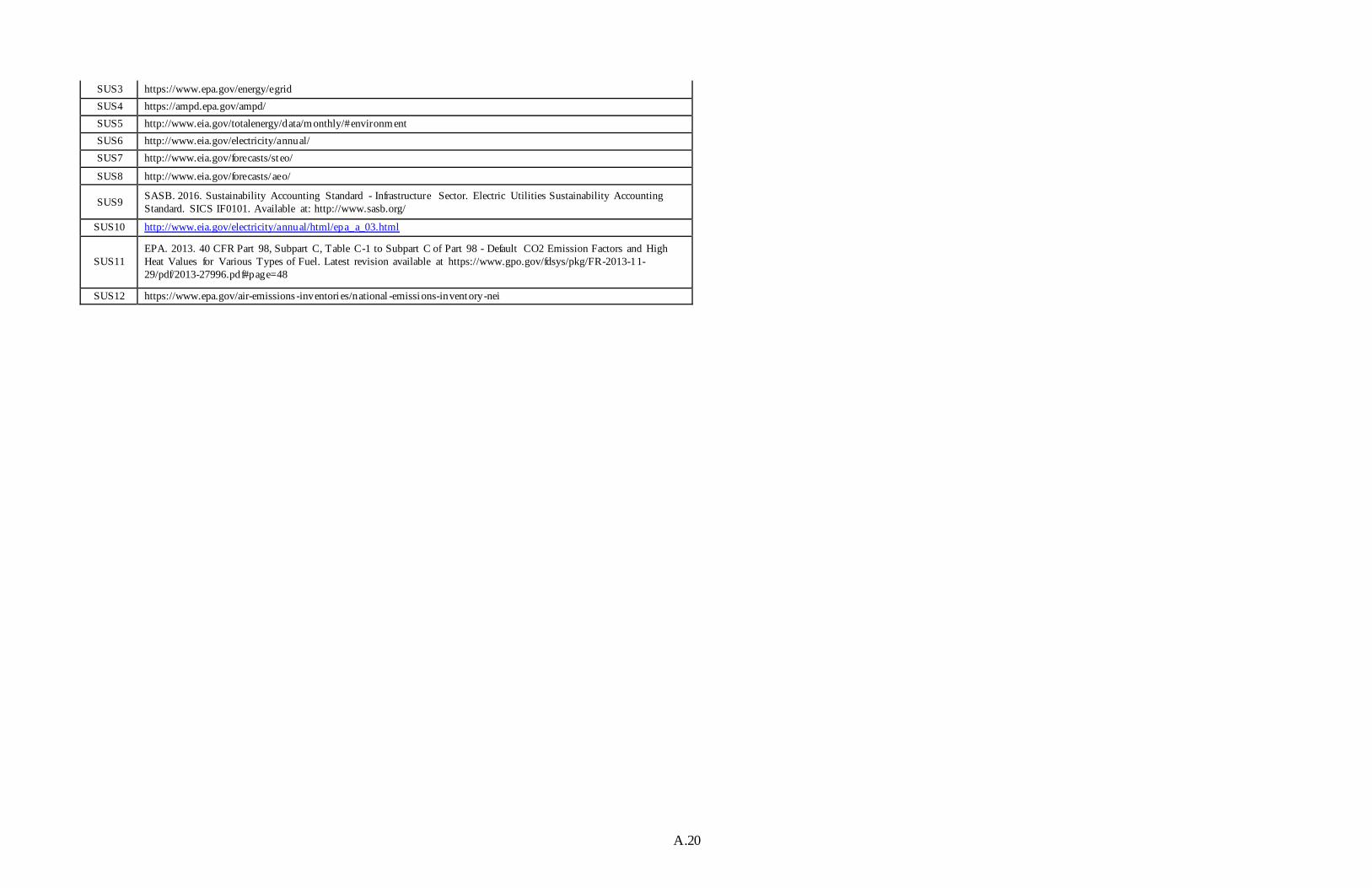
A.20
SUS3 https://www.epa.gov/energy/egrid
SUS4 https://ampd.epa.gov/ampd/
SUS5 http://www.eia.gov/totalenergy/data/monthly/#environment
SUS6 http://www.eia.gov/electricity/annual/
SUS7 http://www.eia.gov/forecasts/st eo/
SUS8 http://www.eia.gov/forecasts/ aeo/
SUS9 SASB. 2016. Sustainability Accounting Standard - Infrastructure Sector. Electric Utilities Sustainability Accounting
Standard. SICS IF0101. Available at: http://www.sasb.org/
SUS10 http://www.eia.gov/electricity/annual/html/epa_a_03.html
SUS11
EPA. 2013. 40 CFR Part 98, Subpart C, Table C-1 to Subpart C of Part 98 - Default CO2 Emission Factors and High
Heat Values for Various Types of Fuel. Latest revision available at https://www.gpo.gov/fdsys/pkg/FR-2013-11-
29/pdf/2013-27996.pdf#page=48
SUS12 https://www.epa.gov/air-emissions -inventori es/national -emissions-inventory-nei

A.21
A.5 Affordability
A.5.1 Data
Categorization Summary Historical Supporting Data - Lagging Metrics
Metric
# Sector
Category
(from list)
Electric System
Infrastructure
Component
(from list)
Metrics
Name Description Motivation Units
Metric
Type
(from
List)
Metric
Classification
(from List)
Metric Use
(from List)
Primary
User
(from
List)
Secondary
User
(from List -
if
applicable)
Metrics
Tense
(Lagging/
Leading)
Applicable
to
Valuation
Project
(Yes/No)
Data
Available?
(Yes/No)
Geospatial
Resolution
(from list)
Temporal
Frequency of
Data Reporting
(from list)
Citation/Data
Source
Reference #
Potential Issues
Comments
1 Electricity Affordability All Levelized cost
of electricity
(LCOE)
total cost of installing
and operating a project
expressed in dollars per
kilowatt-hour of
electricity generated by
the system over its life
LCOE has been used for
calculating the cost-
effectiveness of projects.
By incorporating
different categories of
cash flows, different
stakeholder interests can
be examined.
$/MWh,
$/kWh
Absolute Outcome Decision
making
Ultility Regulator Leading Yes AFF1
2 Electricity Affordability All Internal Rate
of Return
(IRR)
the discount rate that
makes the NPV of the
cost and revenue stream
equal to zero
IRR has been used for
calculating the cost-
effectiveness of projects.
By incorporating
different categories of
cash flows, different
stakeholder interests can
be examined. Rational
investors would
undertake projects as
ranked by descending
IRR order.
Percentage Absolute Outcome Decision
making
Ultility Regulator Leading Yes AFF1
3 Electricity Affordability All Simple
Payback
Period (SPP)
the length of time after
the first investment that
the undiscounted sum of
costs and revenues equals
zero
Easy to understand
representation of cost
effectiveness
# of years or
months
Absolute Outcome Decision
making
Ultility Regulator Leading Yes AFF2 While simple to calculate, it
does not give as meaningful a
result as the NPV or IRR,
because it only tells how long
it takes until the costs have
been recovered, without
providing an estimation of the
total return. It does not capture
any information about the time
value of money, nor the impact
over the full life of the project.
4 Electricity Affordability All Net Revenue
Requirements
the annual stream of
revenue necessary to
recover the total costs of
a project including
capital (in the form of
depreciation), operating
costs including fuel,
financing costs including
interest and required
return on rate on equity,
and taxes including both
costs and incentives.
Revenue requirements
are typically calculated
and used on a company-
wide basis, but the
impacts of single
projects on revenue
requirements can be
calculated by applying
the rules on just the
subset of costs
applicable to the project.
$/year Absolute Outcome Decision
making
Ultility Regulator Leading Yes AFF3
5 Electricity Affordability All Avoided Cost net change in the costs of
the overall system with
the development of the
specified project
used by utilities and
regulators for
establishing the value of
a project compared to its
alternatives and for
setting the value of
distributed generation
technologies
$ Absolute Outcome Decision
making
Ultility Regulator Leading Yes AFF1 It can be a complicated
calculation, subject to defining
the boundaries of the analysis
and adequately simulating the
system. It captures items such
as the energy avoided from
other generators because of the
new project (either a generator,
demand response, or energy
efficiency measures), capacity,
substation, or transmission and
distribution expansion

A.22
Categorization Summary Historical Supporting Data - Lagging Metrics
Metric
# Sector
Category
(from list)
Electric System
Infrastructure
Component
(from list)
Metrics
Name Description Motivation Units
Metric
Type
(from
List)
Metric
Classification
(from List)
Metric Use
(from List)
Primary
User
(from
List)
Secondary
User
(from List -
if
applicable)
Metrics
Tense
(Lagging/
Leading)
Applicable
to
Valuation
Project
(Yes/No)
Data
Available?
(Yes/No)
Geospatial
Resolution
(from list)
Temporal
Frequency of
Data Reporting
(from list)
Citation/Data
Source
Reference #
Potential Issues
Comments
6 Electricity Affordability All Customer cost
burden
Proportion of customer
income devoted to
purchasing desired level
of electricty service
Foundational to
estimating customer
affordability
fraction Numerical
or
intensity
Outcome Learning/
Demonstration
Regulator Consumer
advocate;
other
advocacy
groups
Lagging Yes Yes National,
Interconnection,
RTO, State, Utility
service area,
Distribution system
footprint
Annual/ monthly AFF4 Straightforward estimation for
residential sector; more
complicated for commercial
and industrial sectors; public
data sources for customer cost
may have limitations
compared to actual billing
data.
7 Electricity Affordability All Affordability
gap factor
Indication of the
difference between
affordable customer costs
and observed customer
costs
Provides scale to the
affordability question -
How unaffordable are
electricity costs on
average?
factor or
fraction
Numerical
or
intensity
Outcome Learning/
Demonstration
Regulator Consumer
advocate;
other
advocacy
groups
Lagging Yes Yes National,
Interconnection,
RTO, State, Utility
service area,
Distribution system
footprint
Annual/ monthly AFF4, AFF5,
AFF6
Straightforward estimation for
residential sector; more
complicated for commercial
and industrial sectors; public
data sources for customer cost
may have limitations
compared to actual billing
data.
8 Electricity Affordability All Affordability
gap headcount
Number of households
facing costs higher than
an established affordable
threshold
Provides scale to the
affordability question -
How many customers
face unaffordable
electricity?
#
Households
or % of
households
Absolute Outcome Learning/
Demonstration
Regulator Consumer
advocate;
other
advocacy
groups
Lagging Yes Yes National,
Interconnection,
RTO, State, Utility
service area,
Distribution system
footprint
Annual/ monthly AFF4, AFF7 Straightforward estimation for
residential sector; more
complicated for commercial
and industrial sectors; public
data sources for customer cost
may have limitations
compared to actual billing
data.
9 Electricity Affordability All Affordability
gap index
temporal index of
affordability gap factor
compared to a base year
Answers the question: Is
electricity becoming
more or less affordable?
index Numerical Outcome Learning/
Demonstration
Regulator Consumer
advocate;
other
advocacy
groups
Lagging Yes Yes National,
Interconnection,
RTO, State, Utility
service area,
Distribution system
footprint
Annual/ monthly AFF4, AFF7 Straightforward estimation for
residential sector; more
complicated for commercial
and industrial sectors; public
data sources for customer cost
may have limitations
compared to actual billing
data.
10 Electricity Affordability All Affordability
gap headcount
index
temporal index of
affordability gap
headcount compared to a
base year
Answers the question:
Are more or less
customers facing
unaffordable electricity
costs?
index Numerical Outcome Learning/
Demonstration
Regulator Consumer
advocate;
other
advocacy
groups
Lagging Yes Yes National,
Interconnection,
RTO, State, Utility
service area,
Distribution system
footprint
Annual/ monthly AFF4, AFF7 Straightforward estimation for
residential sector; more
complicated for commercial
and industrial sectors; public
data sources for customer cost
may have limitations
compared to actual billing
data.

A.23
A.5.2 References
Citation/
Data
Source
Ref # Citation/Data Source
AFF1
Short W., Packey DJ, & Holt T. 1995. A Manual for the Economic Evaluation of Energy Efficiency and Renewable Energy
Technologies. NREL/TP-462-5173, National Renewable Energy Laboratory, Golden, Colorado. Available at:
http://www.nrel.gov/docs/legosti/old/5173.pdf
AFF2
Hart R & Liu B. 2015. Methodology for Evaluating Cost-effectiveness of Commercial Energy Code Changes. PNNL-23923, Rev 1,
Pacific Northwest National Laboratory, Richland, Washington. Available online at:
https://www.energycodes.gov/sit es/default/ files/documents/ commercial_methodology.pdf
AFF3 Hadley SW, Hill LJ, and Perlack RD. 1993. Report on the Study of Tax and Rate Treatment of Renewable Energy Projects. ORNL-
6772, Oak Ridge National Laboratory, Oak Ridge, Tennessee. Available at: http://www.ornl.gov/~webworks/ cpr/v823/ rpt/68456.pdf
AFF4 Colton (2011) http://www.nyserda.ny.gov/-/media/Files/EDPPP/LIFE/Resources/2008 -2010-affordability-gap.pdf
AFF5 Drehobl and Ross (2016) Lifting the High Energy Burden in America’s Largest Cities: How Energy Efficiency Can Improve Low
Income and Underserved Communities. American Council for an Energy Efficient Economy, City, State.
AFF6 Heindl and Schuessler (2015) Dynamic properties of energy affordability measures. Energy Policy 86:123–132.
AFF7 Fisher, Sheehan, and Colton. 2013. “ Home Energy Affordability Gap.” Accessed online at:
http://www.homeenergyaffordabilitygap.com/.

A.24
A.6 Security
A.6.1 Data
Categorization Summary Historical Supporting Data - Lagging Metrics
Metric # Sector
Category
(from list)
Electric
System
Infrastructure
Component
(from list) Metrics Name Description Motivation Units
Metric Type
(from List)
Metric
Classific-
ation
(from
List)
Metric
Use
(from
List)
Primary
User
(from
List)
Secondary
User
(from
List -
if applicable)
Metrics
Tense
(Lagging/
Leading)
Applicable
to
Valuation
Project
(Yes/No)
Data
Available?
(Yes/No)
Geospatial
Resolution
(from list)
Temporal
Frequency of
Data Reporting
(from list) Citation/Data Source Reference #
Potential
Issues
Comments
1 Electrici
ty
Security All Physical
Security
Accounts for presence of
physical security measures
such as fences, gates, etc.
Documents utility's
current CIKR
protection posture
and overall security
awareness
0 to 100% Numerical Process Account-
ability
Utility State
Regulator
Lagging YES YES
(public &
DHS)
Distribution
system
footprint
Annual Argonne National Laboratory, 2009.
Constructing Vulnerability and Protective
Measures Indices for the Enhanced Critical
Infrastructure Protection Program, available
at
http://www.ipd.anl.gov/anlpubs/2009/10/65
406.pdf
Go Cubs Go!
2 Electrici
ty
Security All Security Force Staffing, equipment,
weaponry, training, patrols,
after hour security, etc.
Documents utility's
current CIKR
protection posture
and overall security
awareness
0 to 100% Numerical Process Account-
ability
Utility State
Regulator
Lagging YES YES
(public &
DHS)
Distribution
system
footprint
Annual Argonne National Laboratory, 2009.
Constructing Vulnerability and Protective
Measures Indices for the Enhanced Critical
Infrastructure Protection Program, available
at
http://www.ipd.anl.gov/anlpubs/2009/10/65
406.pdf
3 Electrici
ty
Security All Security
Management
Business continuity plan,
security plan, threat levels,
background checks, etc.
Documents utility's
current CIKR
protection posture
and overall security
awareness
0 to 100% Numerical Process Account-
ability
Utility State
Regulator
Leading YES YES
(public &
DHS)
Distribution
system
footprint
Annual Argonne National Laboratory, 2009.
Constructing Vulnerability and Protective
Measures Indices for the Enhanced Critical
Infrastructure Protection Program, available
at
http://www.ipd.anl.gov/anlpubs/2009/10/65
406.pdf
4 Electrici
ty
Security All Information
Sharing
Threat sources and
information sharing
mechanisms
Documents utility's
current CIKR
protection posture
and overall security
awareness
0 to 100% Numerical Process Account-
ability
Utility State
Regulator
Leading YES YES
(public &
DHS)
Distribution
system
footprint
Annual Argonne National Laboratory, 2009.
Constructing Vulnerability and Protective
Measures Indices for the Enhanced Critical
Infrastructure Protection Program, available
at
http://www.ipd.anl.gov/anlpubs/2009/10/65
406.pdf
5 Electrici
ty
Security All Security
Activity
History/
Background
New protective measures,
random security measures,
etc.
Documents utility's
current CIKR
protection posture
and overall security
awareness
0 to 100% Numerical Process Account-
ability
Utility State
Regulator
Lagging YES YES
(public &
DHS)
Distribution
system
footprint
Annual Argonne National Laboratory, 2009.
Constructing Vulnerability and Protective
Measures Indices for the Enhanced Critical
Infrastructure Protection Program, available
at
http://www.ipd.anl.gov/anlpubs/2009/10/65
406.pdf

A.25
Categorization Summary Historical Supporting Data - Lagging Metrics
Metric # Sector
Category
(from list)
Electric
System
Infrastructure
Component
(from list) Metrics Name Description Motivation Units
Metric Type
(from List)
Metric
Classific-
ation
(from
List)
Metric
Use
(from
List)
Primary
User
(from
List)
Secondary
User
(from
List -
if applicable)
Metrics
Tense
(Lagging/
Leading)
Applicable
to
Valuation
Project
(Yes/No)
Data
Available?
(Yes/No)
Geospatial
Resolution
(from list)
Temporal
Frequency of
Data Reporting
(from list) Citation/Data Source Reference #
Potential
Issues
Comments
6 Electrici
ty
Security All BES Security
Metric 1:
Reportable
Cyber Security
Incidents
The number of reportable
cyber security incidents that
result in a loss of load,
summed on a quarterly
basis; this is a lagging
metric
Describes how
prepared the electric
sector is to a physical
attack.
≥0
(dimensionless)
Numerical Process Account-
ability
NERC Lagging NO YES (from
NERC)
National Quarterly NERC, 2015. Bulk Electric System
Security Metrics Working Draft, available
at
http://www.nerc.com/comm/CIPC/Bulk%2
0Electric%20System%20Security%20Metri
cs%20Working%20G1/BES_Security_Metr
ics_CIPC_March_2015.pdf
This metric is
applied at the
national level
and there is
insufficient
public data
for its
application at
the utility- or
State-level.
7 Electrici
ty
Security All BES Security
Metric 2:
Reportable
Physical
Security
Events
The number of physical
security reportable events
that occur over time as a
result of threats to a facility
or BES control center or
damage or destruction to a
facility, summed on a
quarterly basis; this is a
lagging metric
Describes how
prepared the electric
sector is to a physical
attack.
≥0
(dimensionless)
Numerical Process Account-
ability
NERC Lagging NO YES (from
NERC)
National Quarterly NERC, 2015. Bulk Electric System
Security Metrics Working Draft, available
at
http://www.nerc.com/comm/CIPC/Bulk%2
0Electric%20System%20Security%20Metri
cs%20Working%20G1/BES_Security_Metr
ics_CIPC_March_2015.pdf
This metric is
applied at the
national level
and there is
insufficient
public data
for its
application at
the utility- or
State-level.
8 Electrici
ty
Security All BES Security
Metric 3: ES-
ISAC
Membership
The number of ES-ISAC
member organizations,
summed on a quarterly
basis; this is a leading
metric.
Describes how
prepared the electric
sector is to a physical
attack.
≥0
(dimensionless)
Numerical Process Decision
making
NERC Leading NO YES (from
NERC)
National Quarterly NERC, 2015. Bulk Electric System
Security Metrics Working Draft, available
at
http://www.nerc.com/comm/CIPC/Bulk%2
0Electric%20System%20Security%20Metri
cs%20Working%20G1/BES_Security_Metr
ics_CIPC_March_2015.pdf
This metric
could be
applied at the
utility-level.
9 Electrici
ty
Security All BES Security
Metric 4:
Industry-
Sourced
Information
Sharing
The number of ES-ISAC
Incident Bulletins
[currently known as
Watchlist entries], summed
on a quarterly basis; this is
a leading metric.
Describes how
prepared the electric
sector is to a physical
attack.
≥0
(dimensionless)
Numerical Process Decision
making
NERC Leading NO YES (from
NERC)
National Quarterly NERC, 2015. Bulk Electric System
Security Metrics Working Draft, available
at
http://www.nerc.com/comm/CIPC/Bulk%2
0Electric%20System%20Security%20Metri
cs%20Working%20G1/BES_Security_Metr
ics_CIPC_March_2015.pdf
This metric is
applied at the
national level
and there is
insufficient
public data
for its
application at
the utility- or
State-level.
10 Electrici
ty
Security All BES Security
Metric 5:
Global Cyber
Vulnerabilities
The number of global cyber
vulnerabilities with a CVSS
[Common Vulnerability
Scoring System, NIST
2015] of 7 or higher; this is
a lagging metric.
Describes how
prepared the electric
sector is to a physical
attack.
≥0
(dimensionless)
Numerical Process Account-
ability
NERC Lagging NO YES (from
NERC)
National Quarterly NERC, 2015. Bulk Electric System
Security Metrics Working Draft, available
at
http://www.nerc.com/comm/CIPC/Bulk%2
0Electric%20System%20Security%20Metri
cs%20Working%20G1/BES_Security_Metr
ics_CIPC_March_2015.pdf
This metric is
applied at the
national level
and there is
insufficient
public data
for its
application at
the utility- or
State-level.
11 Electrici
ty
Security Distribution Number of
instances of
copper theft
Tracks the impact of copper
theft and vandalism
Describes how
prepared the electric
sector is to a physical
attack.
≥0
(dimensionless)
Numerical Process Account-
ability
Utility State
Regulator
Lagging NO Proprietary
utility data
Utility Monthly CPUC, 2015. Regulation of Physical
Security for the Electric Distribution
System, available at
http://www.cpuc.ca.gov/NR/rdonlyres/930F
CC00-BE2F-4BCF-9B68-
2CA2CDC38186/0/PhysicalSecurityforthe
UtilityIndustry20150210.pdf
This metrics
depends on
proprietary
utility data
that is
difficult to
collect
12 Electrici
ty
Security Distribution Number of
successful or
unsuccessful
intrusion or
attack
This metric captures the
total number of attacks
against a given utility's
facilities
Describes how
prepared the electric
sector is to a physical
attack.
≥0
(dimensionless)
Numerical Process Account-
ability
Utility State
Regulator
Lagging NO Proprietary
utility data
Utility Monthly CPUC, 2015. Regulation of Physical
Security for the Electric Distribution
System, available at
http://www.cpuc.ca.gov/NR/rdonlyres/930F
CC00-BE2F-4BCF-9B68-
2CA2CDC38186/0/PhysicalSecurityforthe
UtilityIndustry20150210.pdf
This metrics
depends on
proprietary
utility data
that is
difficult to
collect

A.26
Categorization Summary Historical Supporting Data - Lagging Metrics
Metric # Sector
Category
(from list)
Electric
System
Infrastructure
Component
(from list) Metrics Name Description Motivation Units
Metric Type
(from List)
Metric
Classific-
ation
(from
List)
Metric
Use
(from
List)
Primary
User
(from
List)
Secondary
User
(from
List -
if applicable)
Metrics
Tense
(Lagging/
Leading)
Applicable
to
Valuation
Project
(Yes/No)
Data
Available?
(Yes/No)
Geospatial
Resolution
(from list)
Temporal
Frequency of
Data Reporting
(from list) Citation/Data Source Reference #
Potential
Issues
Comments
13 Electrici
ty
Security Distribution Number of
false or
nuisance
alarms
Collection of the number of
non-attack-related incidents
for a given utility
Describes how
prepared the electric
sector is to a physical
attack.
≥0
(dimensionless)
Numerical Process Account-
ability
Utility State
Regulator
Lagging NO Proprietary
utility data
Utility Monthly CPUC, 2015. Regulation of Physical
Security for the Electric Distribution
System, available at
http://www.cpuc.ca.gov/NR/rdonlyres/930F
CC00-BE2F-4BCF-9B68-
2CA2CDC38186/0/PhysicalSecurityforthe
UtilityIndustry20150210.pdf
This metrics
depends on
proprietary
utility data
that is
difficult to
collect
14 Electrici
ty
Security Distribution Condition of
all monitoring
equipment
The number of times that
the security system is
unable to respond and
detect a physical security
incident.
Describes how
prepared the electric
sector is to a physical
attack.
Qualitative Qualitative Process Decision
making
Utility State
Regulator
Lagging NO Proprietary
utility data
Utility Monthly CPUC, 2015. Regulation of Physical
Security for the Electric Distribution
System, available at
http://www.cpuc.ca.gov/NR/rdonlyres/930F
CC00-BE2F-4BCF-9B68-
2CA2CDC38186/0/PhysicalSecurityforthe
UtilityIndustry20150210.pdf
This metrics
depends on
proprietary
utility data
that is
difficult to
collect
15 Electrici
ty
Security Distribution Performance
of security
personnel in
training
exercises and
on tests
Describes how prepared the
electric sector is for a
physical attack.
Describes how
prepared the electric
sector is to a physical
attack.
Qualitative Qualitative Process Decision
making
Utility State
Regulator
Lagging NO Proprietary
utility data
Utility Monthly CPUC, 2015. Regulation of Physical
Security for the Electric Distribution
System, available at
http://www.cpuc.ca.gov/NR/rdonlyres/930F
CC00-BE2F-4BCF-9B68-
2CA2CDC38186/0/PhysicalSecurityforthe
UtilityIndustry20150210.pdf
This metrics
depends on
proprietary
utility data
that is
difficult to
collect
16 Electrici
ty
Security Distribution Number of
problems
found with
condition of
deterrence and
monitoring
measures
Describes how prepared the
electric sector is for a
physical attack.
Describes how
prepared the electric
sector is to a physical
attack.
≥0
(dimensionless)
Numerical Process Account-
ability
Utility State
Regulator
Lagging NO Proprietary
utility data
Utility Monthly CPUC, 2015. Regulation of Physical
Security for the Electric Distribution
System, available at
http://www.cpuc.ca.gov/NR/rdonlyres/930F
CC00-BE2F-4BCF-9B68-
2CA2CDC38186/0/PhysicalSecurityforthe
UtilityIndustry20150210.pdf
This metrics
depends on
proprietary
utility data
that is
difficult to
collect
17 Electrici
ty
Security Distribution Number of
instances of
vandalism or
graffiti
Tracks the impact of copper
theft and vandalism
Describes how
prepared the electric
sector is for a
physical attack.
≥0
(dimensionless)
Numerical Process Account-
ability
Utility State
Regulator
Lagging NO Proprietary
utility data
Utility Monthly CPUC, 2015. Regulation of Physical
Security for the Electric Distribution
System, available at
http://www.cpuc.ca.gov/NR/rdonlyres/930F
CC00-BE2F-4BCF-9B68-
2CA2CDC38186/0/PhysicalSecurityforthe
UtilityIndustry20150210.pdf
This metrics
depends on
proprietary
utility data
that is
difficult to
collect
18 Electrici
ty
Security Distribution Number of
problems with
access control
Identifies the number of
times that an intruder tries
to access electric sector
facilities for a given utility
Describes how
prepared the electric
sector is to a physical
attack.
≥0
(dimensionless)
Numerical Process Account-
ability
Utility State
Regulator
Lagging NO Proprietary
utility data
Utility Monthly CPUC, 2015. Regulation of Physical
Security for the Electric Distribution
System, available at
http://www.cpuc.ca.gov/NR/rdonlyres/930F
CC00-BE2F-4BCF-9B68-
2CA2CDC38186/0/PhysicalSecurityforthe
UtilityIndustry20150210.pdf
This metrics
depends on
proprietary
utility data
that is
difficult to
collect
19 Electrici
ty
Security Distribution Number of
malfunctions
of security
equipment or
camera
coverage
The number of times that
the security system is
unable to respond and
detect a physical security
incident.
Describes how
prepared the electric
sector is to a physical
attack.
≥0
(dimensionless)
Numerical Process Account-
ability
Utility State
Regulator
Lagging NO Proprietary
utility data
Utility Monthly CPUC, 2015. Regulation of Physical
Security for the Electric Distribution
System, available at
http://www.cpuc.ca.gov/NR/rdonlyres/930F
CC00-BE2F-4BCF-9B68-
2CA2CDC38186/0/PhysicalSecurityforthe
UtilityIndustry20150210.pdf
This metrics
depends on
proprietary
utility data
that is
difficult to
collect
20 Electrici
ty
Security All Incidents
Requiring
Manual
Cleanup.
Number of Incidents
Requiring Manual Cleanup.
Describes how
prepared the electric
sector is to a cyber
attack.
Numerical Process Account-
ability
Utility State
Regulator
Lagging NO Proprietary
company
data
Company-
level
Monthly EPRI, 2015. "Creating Security Metrics for
the Electric Sector," available at
http://www.epri.com/abstracts/Pages/Produ
ctAbstract.aspx?ProductId=0000000030020
05947
This metrics
depends on
proprietary
utility data
that is
difficult to
collect

A.27
Categorization Summary Historical Supporting Data - Lagging Metrics
Metric # Sector
Category
(from list)
Electric
System
Infrastructure
Component
(from list) Metrics Name Description Motivation Units
Metric Type
(from List)
Metric
Classific-
ation
(from
List)
Metric
Use
(from
List)
Primary
User
(from
List)
Secondary
User
(from
List -
if applicable)
Metrics
Tense
(Lagging/
Leading)
Applicable
to
Valuation
Project
(Yes/No)
Data
Available?
(Yes/No)
Geospatial
Resolution
(from list)
Temporal
Frequency of
Data Reporting
(from list) Citation/Data Source Reference #
Potential
Issues
Comments
21 Electrici
ty
Security All Mean-Time-to-
Fix (MTTF).
Mean-Time-to-Fix
(MTTF).
Describes how
prepared the electric
sector is to a cyber
attack.
≥0
(dimensionless)
Numerical Process Decision
making
Utility State
Regulator
Lagging NO Proprietary
company
data
Company-
level
Monthly EPRI, 2015. "Creating Security Metrics for
the Electric Sector," available at
http://www.epri.com/abstracts/Pages/Produ
ctAbstract.aspx?ProductId=0000000030020
05947
This metrics
depends on
proprietary
utility data
that is
difficult to
collect
22 Electrici
ty
Security All Cyber Security
Workforce
Management
Cyber Security Workforce
Management
Describes how
prepared the electric
sector is to a cyber
attack.
N/A Qualitative Process Decision
making
Utility State
Regulator
Leading NO Proprietary
company
data
Company-
level
Monthly EPRI, 2015. "Creating Security Metrics for
the Electric Sector," available at
http://www.epri.com/abstracts/Pages/Produ
ctAbstract.aspx?ProductId=0000000030020
05947
This metrics
depends on
proprietary
utility data
that is
difficult to
collect
23 Electrici
ty
Security All Mean Cost to
Mitigate
Vulnerabilities
.
Mean Cost to Mitigate
Vulnerabilities.
Describes how
prepared the electric
sector is to a cyber
attack.
≥0
(dimensionless)
Numerical Process Account-
ability
Utility State
Regulator
Lagging NO Proprietary
company
data
Company-
level
Monthly EPRI, 2015. "Creating Security Metrics for
the Electric Sector," available at
http://www.epri.com/abstracts/Pages/Produ
ctAbstract.aspx?ProductId=0000000030020
05947
This metrics
depends on
proprietary
utility data
that is
difficult to
collect
24 Electrici
ty
Security All Percent of
Changes with
Security
Review.
Percent of Changes with
Security Review.
Describes how
prepared the electric
sector is to a cyber
attack.
≥0
(dimensionless)
Numerical Process Decision
making
Utility State
Regulator
Lagging NO Proprietary
company
data
Company-
level
Monthly EPRI, 2015. "Creating Security Metrics for
the Electric Sector," available at
http://www.epri.com/abstracts/Pages/Produ
ctAbstract.aspx?ProductId=0000000030020
05947
This metrics
depends on
proprietary
utility data
that is
difficult to
collect
25 Electrici
ty
Security All Number of
outgoing
viruses caught
at gateway.
Number of outgoing viruses
caught at gateway.
Under investigation
by EPRI
≥0
(dimensionless)
Numerical Process Account-
ability
Utility State
Regulator
Lagging NO Proprietary
company
data
Company-
level
Monthly EPRI, 2015. "Creating Security Metrics for
the Electric Sector," available at
http://www.epri.com/abstracts/Pages/Produ
ctAbstract.aspx?ProductId=0000000030020
05947
This metrics
depends on
proprietary
utility data
that is
difficult to
collect
26 Electrici
ty
Security All Mean Time to
Incident
Discovery.
Mean Time to Incident
Discovery.
Under investigation
by EPRI
≥0
(dimensionless)
Numerical Process Decision
making
Utility State
Regulator
Lagging NO Proprietary
company
data
Company-
level
Monthly EPRI, 2015. "Creating Security Metrics for
the Electric Sector," available at
http://www.epri.com/abstracts/Pages/Produ
ctAbstract.aspx?ProductId=0000000030020
05947
This metrics
depends on
proprietary
utility data
that is
difficult to
collect
27 Electrici
ty
Security All Number of
cyber security
skills mastered
per employee.
Number of cyber security
skills mastered per
employee.
Under investigation
by EPRI
≥0
(dimensionless)
Numerical Process Account-
ability
Utility State
Regulator
Lagging NO Proprietary
company
data
Company-
level
Monthly EPRI, 2015. "Creating Security Metrics for
the Electric Sector," available at
http://www.epri.com/abstracts/Pages/Produ
ctAbstract.aspx?ProductId=0000000030020
05947
This metrics
depends on
proprietary
utility data
that is
difficult to
collect
28 Electrici
ty
Security All Mean Time
between
Security
Incidents.
Mean Time between
Security Incidents.
Under investigation
by EPRI
≥0
(dimensionless)
Numerical Process Decision
making
Utility State
Regulator
Lagging NO Proprietary
company
data
Company-
level
Monthly EPRI, 2015. "Creating Security Metrics for
the Electric Sector," available at
http://www.epri.com/abstracts/Pages/Produ
ctAbstract.aspx?ProductId=0000000030020
05947
This metrics
depends on
proprietary
utility data
that is
difficult to
collect
29 Electrici
ty
Security All Cost of
Incidents.
Cost of Incidents. Under investigation
by EPRI
≥0
(dimensionless)
Numerical Process Account-
ability
Utility State
Regulator
Lagging NO Proprietary
company
data
Company-
level
Monthly EPRI, 2015. "Creating Security Metrics for
the Electric Sector," available at
http://www.epri.com/abstracts/Pages/Produ
ctAbstract.aspx?ProductId=0000000030020
05947
This metrics
depends on
proprietary
utility data
that is
difficult to
collect

A.28
Categorization Summary Historical Supporting Data - Lagging Metrics
Metric # Sector
Category
(from list)
Electric
System
Infrastructure
Component
(from list) Metrics Name Description Motivation Units
Metric Type
(from List)
Metric
Classific-
ation
(from
List)
Metric
Use
(from
List)
Primary
User
(from
List)
Secondary
User
(from
List -
if applicable)
Metrics
Tense
(Lagging/
Leading)
Applicable
to
Valuation
Project
(Yes/No)
Data
Available?
(Yes/No)
Geospatial
Resolution
(from list)
Temporal
Frequency of
Data Reporting
(from list) Citation/Data Source Reference #
Potential
Issues
Comments
30 Electrici
ty
Security All Percentage of
Systems
without
Known Severe
Vulnerabilities
.
Percentage of Systems
without Known Severe
Vulnerabilities.
Under investigation
by EPRI
≥0
(dimensionless)
Numerical Process Account-
ability
Utility State
Regulator
Lagging NO Proprietary
company
data
Company-
level
Monthly EPRI, 2015. "Creating Security Metrics for
the Electric Sector," available at
http://www.epri.com/abstracts/Pages/Produ
ctAbstract.aspx?ProductId=0000000030020
05947
This metrics
depends on
proprietary
utility data
that is
difficult to
collect
31 Electrici
ty
Security All Mean Time to
Patch.
Mean Time to Patch. Under investigation
by EPRI
≥0
(dimensionless)
Numerical Process Account-
ability
Utility State
Regulator
Lagging NO Proprietary
company
data
Company-
level
Monthly EPRI, 2015. "Creating Security Metrics for
the Electric Sector," available at
http://www.epri.com/abstracts/Pages/Produ
ctAbstract.aspx?ProductId=0000000030020
05947
This metrics
depends on
proprietary
utility data
that is
difficult to
collect
32 Electrici
ty
Security All Percentage of
Changes with
Security
Exceptions.
Percentage of Changes with
Security Exceptions.
Under investigation
by EPRI
≥0
(dimensionless)
Numerical Process Accounta
bility
Utility State
Regulator
Lagging NO Proprietary
company
data
Company-
level
Monthly EPRI, 2015. "Creating Security Metrics for
the Electric Sector," available at
http://www.epri.com/abstracts/Pages/Produ
ctAbstract.aspx?ProductId=0000000030020
05947
This metrics
depends on
proprietary
utility data
that is
difficult to
collect
33 Electrici
ty
Security All Percentage of
Applications
Subject to Risk
Assessment.
Percentage of Applications
Subject to Risk
Assessment.
Under investigation
by EPRI
≥0
(dimensionless)
Numerical Process Account-
ability
Utility State
Regulator
Lagging NO Proprietary
company
data
Company-
level
Monthly EPRI, 2015. "Creating Security Metrics for
the Electric Sector," available at
http://www.epri.com/abstracts/Pages/Produ
ctAbstract.aspx?ProductId=0000000030020
05947
This metrics
depends on
proprietary
utility data
that is
difficult to
collect
34 Electrici
ty
Security All Information
Security
Budget
Allocation.
Information Security
Budget Allocation.
Under investigation
by EPRI
≥0
(dimensionless)
Numerical Process Decision
making
Utility State
Regulator
Lagging NO Proprietary
company
data
Company-
level
Monthly EPRI, 2015. "Creating Security Metrics for
the Electric Sector," available at
http://www.epri.com/abstracts/Pages/Produ
ctAbstract.aspx?ProductId=0000000030020
05947
This metrics
depends on
proprietary
utility data
that is
difficult to
collect
35 Electrici
ty
Security All Compliance or
Coverage of
Information
Security
Practice
Compliance or Coverage of
Information Security
Practice
Under investigation
by EPRI
N/A Qualitative Process Decision
making
Utility State
Regulator
Lagging NO Proprietary
company
data
Company-
level
Monthly EPRI, 2015. "Creating Security Metrics for
the Electric Sector," available at
http://www.epri.com/abstracts/Pages/Produ
ctAbstract.aspx?ProductId=0000000030020
05947
This metrics
depends on
proprietary
utility data
that is
difficult to
collect
36 Electrici
ty
Security All Number of
protective
programs
implemented
in a given year
Number of protective
programs implemented in a
given year
Describes how
prepared the electric
sector is to a physical
attack.
≥0
(dimensionless)
Numerical Process Account-
ability
Federal
(DHS),
Utility
State
Regulator
Lagging NO Proprietary
company
data
Company-
level
Annual DHS, 2006. National Infrastructure
Protection Plan, available at
https://www.dhs.gov/xlibrary/assets/NIPP_
Plan_noApps.pdf
This metrics
depends on
proprietary
utility data
that is
difficult to
collect
37 Electrici
ty
Security All Level of
investment of
protective
programs
Level of investment of
protective programs
Describes how
prepared the electric
sector is to a physical
attack.
≥0
(dimensionless)
Numerical Process Account-
ability
Federal
(DHS),
Utility
State
Regulator
Lagging NO Proprietary
company
data
Company-
level
Annual DHS, 2006. National Infrastructure
Protection Plan, available at
https://www.dhs.gov/xlibrary/assets/NIPP_
Plan_noApps.pdf
This metrics
depends on
proprietary
utility data
that is
difficult to
collect
38 Electrici
ty
Security All Number of
detection
systems
installed at
faciities
Number of detection
systems installed at faciities
Describes how
prepared the electric
sector is to a physical
attack.
≥0
(dimensionless)
Numerical Process Accounta
bility
Federal
(DHS),
Utility
State
Regulator
Lagging NO Proprietary
company
data
Company-
level
Annual DHS, 2006. National Infrastructure
Protection Plan, available at
https://www.dhs.gov/xlibrary/assets/NIPP_
Plan_noApps.pdf
This metrics
depends on
proprietary
utility data
that is
difficult to
collect

A.29
Categorization Summary Historical Supporting Data - Lagging Metrics
Metric # Sector
Category
(from list)
Electric
System
Infrastructure
Component
(from list) Metrics Name Description Motivation Units
Metric Type
(from List)
Metric
Classific-
ation
(from
List)
Metric
Use
(from
List)
Primary
User
(from
List)
Secondary
User
(from
List -
if applicable)
Metrics
Tense
(Lagging/
Leading)
Applicable
to
Valuation
Project
(Yes/No)
Data
Available?
(Yes/No)
Geospatial
Resolution
(from list)
Temporal
Frequency of
Data Reporting
(from list) Citation/Data Source Reference #
Potential
Issues
Comments
39 Electrici
ty
Security All Proportion of
facility's
workforce that
has completed
security
training
Proportion of facility's
workforce that has
completed security training
Describes how
prepared the electric
sector is to a physical
attack.
≥0
(dimensionless)
Numerical Process Account-
ability
Federal
(DHS),
Utility
State
Regulator
Lagging NO Proprietary
company
data
Company-
level
Annual DHS, 2006. National Infrastructure
Protection Plan, available at
https://www.dhs.gov/xlibrary/assets/NIPP_
Plan_noApps.pdf
This metrics
depends on
proprietary
utility data
that is
difficult to
collect
40 Electrici
ty
Security All Level of
response to a
data call for
asset
information
Level of response to a data
call for asset information
Describes how
prepared the electric
sector is to a physical
attack.
N/A Qualitative Process Decision
making
Federal
(DHS),
Utility
State
Regulator
Leading NO Proprietary
company
data
Company-
level
Annual DHS, 2006. National Infrastructure
Protection Plan, available at
https://www.dhs.gov/xlibrary/assets/NIPP_
Plan_noApps.pdf
This metrics
depends on
proprietary
utility data
that is
difficult to
collect
41 Electrici
ty
Security All Reduction of
risk from one
year to another
Reduction of risk from one
year to another
Describes how
prepared the electric
sector is to a physical
attack.
≥0
(dimensionless)
Numerical Outcome Decision
making
Federal
(DHS),
Utility
State
Regulator
Leading NO Proprietary
company
data
Company-
level
Annual DHS, 2006. National Infrastructure
Protection Plan, available at
https://www.dhs.gov/xlibrary/assets/NIPP_
Plan_noApps.pdf
This metrics
depends on
proprietary
utility data
that is
difficult to
collect
42 Electrici
ty
Security All Overall risk
mitigation
achieved
nationally
Overall risk mitigation
achieved nationally
Describes how
prepared the electric
sector is to a physical
attack.
≥0
(dimensionless)
Numerical Outcome Decision
making
Federal
(DHS),
Utility
State
Regulator
Leading NO Proprietary
company
data
Company-
level
Annual DHS, 2006. National Infrastructure
Protection Plan, available at
https://www.dhs.gov/xlibrary/assets/NIPP_
Plan_noApps.pdf
This metrics
depends on
proprietary
utility data
that is
difficult to
collect
43 Electrici
ty
Security All Risk
Management
Considers actions to (1)
establish cybersecurity risk
management strategy, (2)
manage cybersecurity risk,
(3) management activities
Describes how
prepared the electric
sector is to a cyber
attack.
MIL1 to MIL3 Qualitative Process Account-
ability
Utility Lagging NO Proprietary
company
data
Company-
level
Annual DOE, 2014. Electricity Subsector
Cybersecurity Capability Maturity Model
(ES-C2M2), available at
http://energy.gov/sites/prod/files/2014/02/f7
/ES-C2M2-v1-1-Feb2014.pdf
This metrics
depends on
proprietary
utility data
that is
difficult to
collect
44 Electrici
ty
Security All Asset, Change,
and
Configuration
Management
Considers actions to (1)
manage asset inventory, (2)
manage asset configuration,
(3) manage changes to
assets, (4) management
activities
Describes how
prepared the electric
sector is to a cyber
attack.
MIL1 to MIL3 Qualitative Process Account-
ability
Utility Lagging NO Proprietary
company
data
Company-
level
Annual DOE, 2014. Electricity Subsector
Cybersecurity Capability Maturity Model
(ES-C2M2), available at
http://energy.gov/sites/prod/files/2014/02/f7
/ES-C2M2-v1-1-Feb2014.pdf
This metrics
depends on
proprietary
utility data
that is
difficult to
collect
45 Electrici
ty
Security All Identity and
Access
Management
Addresses (1) establish and
maintain identities, (2)
control access, (3)
management activities
Describes how
prepared the electric
sector is to a cyber
attack.
MIL1 to MIL3 Qualitative Process Account-
ability
Utility Leading NO Proprietary
company
data
Company-
level
Annual DOE, 2014. Electricity Subsector
Cybersecurity Capability Maturity Model
(ES-C2M2), available at
http://energy.gov/sites/prod/files/2014/02/f7
/ES-C2M2-v1-1-Feb2014.pdf
This metrics
depends on
proprietary
utility data
that is
difficult to
collect
46 Electrici
ty
Security All Threat and
Vulnerability
Management
Addresses activities to (1)
identify and respond to
threats, (2) reduce
cybersecurity
vulnerabilities, (3)
management activities
Describes how
prepared the electric
sector is to a cyber
attack.
MIL1 to MIL3 Qualitative Process Account-
ability
Utility Leading NO Proprietary
company
data
Company-
level
Annual DOE, 2014. Electricity Subsector
Cybersecurity Capability Maturity Model
(ES-C2M2), available at
http://energy.gov/sites/prod/files/2014/02/f7
/ES-C2M2-v1-1-Feb2014.pdf
This metrics
depends on
proprietary
utility data
that is
difficult to
collect
47 Electrici
ty
Security All Situational
Awareness
Considers actions to (1)
perform logging, (2)
perform monitoring, (3)
establish and maintain a
common operating picture
Describes how
prepared the electric
sector is to a cyber
attack.
MIL1 to MIL3 Qualitative Process Account-
ability
Utility Leading NO Proprietary
company
data
Company-
level
Annual DOE, 2014. Electricity Subsector
Cybersecurity Capability Maturity Model
(ES-C2M2), available at
http://energy.gov/sites/prod/files/2014/02/f7
/ES-C2M2-v1-1-Feb2014.pdf
This metrics
depends on
proprietary
utility data
that is
difficult to
collect

A.30
Categorization Summary Historical Supporting Data - Lagging Metrics
Metric # Sector
Category
(from list)
Electric
System
Infrastructure
Component
(from list) Metrics Name Description Motivation Units
Metric Type
(from List)
Metric
Classific-
ation
(from
List)
Metric
Use
(from
List)
Primary
User
(from
List)
Secondary
User
(from
List -
if applicable)
Metrics
Tense
(Lagging/
Leading)
Applicable
to
Valuation
Project
(Yes/No)
Data
Available?
(Yes/No)
Geospatial
Resolution
(from list)
Temporal
Frequency of
Data Reporting
(from list) Citation/Data Source Reference #
Potential
Issues
Comments
48 Electrici
ty
Security All Information
Sharing and
Communicatio
ns
Addresses actions to (1)
share cybersecurity
information, (2)
management activities
Describes how
prepared the electric
sector is to a cyber
attack.
MIL1 to MIL3 Qualitative Process Account-
ability
Utility Leading NO Proprietary
company
data
Company-
level
Annual DOE, 2014. Electricity Subsector
Cybersecurity Capability Maturity Model
(ES-C2M2), available at
http://energy.gov/sites/prod/files/2014/02/f7
/ES-C2M2-v1-1-Feb2014.pdf
This metrics
depends on
proprietary
utility data
that is
difficult to
collect
49 Electrici
ty
Security All Event and
Incident
Response,
Continuity of
Operations
Considers activities to (1)
detect cybersecurity events,
(2) escalate cybersecurity
events and declare
incidents, (3) respond to
incidents and escalated
cybersecurity events, (4)
plan for continuity
Describes how
prepared the electric
sector is to a cyber
attack.
MIL1 to MIL3 Qualitative Process Account-
ability
Utility Leading NO Proprietary
company
data
Company-
level
Annual DOE, 2014. Electricity Subsector
Cybersecurity Capability Maturity Model
(ES-C2M2), available at
http://energy.gov/sites/prod/files/2014/02/f7
/ES-C2M2-v1-1-Feb2014.pdf
This metrics
depends on
proprietary
utility data
that is
difficult to
collect
50 Electrici
ty
Security All Supply Chain
and External
Dependencies
Management
Addresses activities to (1)
identify dependencies, (2)
manage dependency risk
Describes how
prepared the electric
sector is to a cyber
attack.
MIL1 to MIL3 Qualitative Process Account-
ability
Utility Leading NO Proprietary
company
data
Company-
level
Annual DOE, 2014. Electricity Subsector
Cybersecurity Capability Maturity Model
(ES-C2M2), available at
http://energy.gov/sites/prod/files/2014/02/f7
/ES-C2M2-v1-1-Feb2014.pdf
This metrics
depends on
proprietary
utility data
that is
difficult to
collect
51 Electrici
ty
Security All Workforce
Management
Considers actions to (1)
assign cybersecurity
responsibilities, (2) control
the workforce life cycle, (3)
develop cybersecurity
workforce, (4) increase
cybersecurity awareness
Describes how
prepared the electric
sector is to a cyber
attack.
MIL1 to MIL3 Qualitative Process Account-
ability
Utility Leading NO Proprietary
company
data
Company-
level
Annual DOE, 2014. Electricity Subsector
Cybersecurity Capability Maturity Model
(ES-C2M2), available at
http://energy.gov/sites/prod/files/2014/02/f7
/ES-C2M2-v1-1-Feb2014.pdf
This metrics
depends on
proprietary
utility data
that is
difficult to
collect
52 Electrici
ty
Security All Cybersecurity
Program
Management
Evaluates actions to (1)
establish cybersecurity
program strategy, (2)
sponsor cybersecurity
program, (3) establish and
maintain cybersecurity
architecture, (4) perform
secure software
development
Describes how
prepared the electric
sector is to a cyber
attack.
MIL1 to MIL3 Qualitative Process Account-
ability
Utility Leading NO Proprietary
company
data
Company-
level
Annual DOE, 2014. Electricity Subsector
Cybersecurity Capability Maturity Model
(ES-C2M2), available at
http://energy.gov/sites/prod/files/2014/02/f7
/ES-C2M2-v1-1-Feb2014.pdf
This metrics
depends on
proprietary
utility data
that is
difficult to
collect
