grid planning by integrate customer...

24th International Conference on Electricity Distribution Glasgow, 12-15 June 2017

Paper 1025

CIRED 2017 1/5

GRID PLANNING BY INTEGRATE CUSTOMER METERS

Niels ANDERSEN Heiko VESTER Tommy Heine BENTSEN SEAS-NVE – Denmark SEAS-NVE – Denmark SEAS-NVE – Denmark [email protected] [email protected] [email protected]

ABSTRACT

The paper present the new possibilities for grid planning by the use of hourly measured data from consumers in combination with other analysis programs and the Power System analysis tool NEPLAN. The use of detailed grid information and measured data for grid planning, instead of the Velander method, which estimates the load coincidence factors of prosumers and the loads.

INTRODUCTION

The SEAS-NVE distribution company aims to deliver reliable power to customers and simultaneously decrease the costs by intelligent grid development. Besides that, SEAS-NVE is obliged to connect the fast developing renewable energy producers to the grid. During 2009-2012 SEAS-NVE changed the traditional meters to automatic remote meters (AMR) for all customers, which gives access to hourly energy measurements. In 2013, SEAS-NVE developed a software platform to collect and monitor the huge amount of data from more than 400.000 customers fed into more than 110 50/10 kV substations without having measurements from the approximately 11000 10/0.4kV transformers. The collection of data also gives the possibility to include theses in grid planning and both compare and validate the other measuring system. The AMR data combined with other information, measuring and data systems, enables higher accuracy modelling in the grid. The connection of new loads or generators are also improved. The presentation is limited to one 50/10 kV station called Mern (MRN), shown in Figure 1 with approximately 3600 meters/customers and 120 10/0.4kV distribution transformers. For the 10kV grid planning, each 10/0.4kV distribution transformer is modelled as a load, negative for generation. Radial Wind PV Velander Meas.

kWh other Load Load

MRN‐A30 0,0 ‐268,9 2419 1746

MRN‐B30 ‐424,3 ‐70,2 1182 1273

MRN‐D2B ‐223,7 ‐79,3 1273 1055

MRN‐K2M 0,0 ‐174,7 2182 1710

MRN‐B15 ‐3919,2 ‐34,3 818 3546

Total ‐4567,3 ‐627,4 7873 5347Table 1 Load and generation at MERN substation 50 kV substation

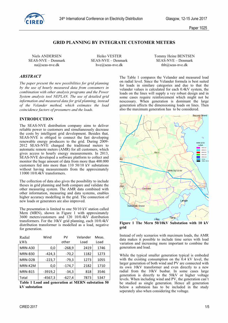
The Table 1 compares the Velander and measured load on radial level. Since the Velander formula is best suited for loads in similare categories and due to that the velander values is calculated for each 0.4kV system, the loads on the lines will supply a vey robust design and in some cases require reinforcement which might not be nescessary. When generation is dominant the large generation affects the dimensioning loads on lines. Then also the maximum generation has to be considered.

Figure 1 The Mern 50/10kV Substation with 10 kV grid Instead of only scenarios with maximum loads, the AMR data makes it possible to include time series with load variation and increasing more important to combine the generation and load. While the typical smaller generation typical is embeded with the existing consumption on the 0.4 kV level, the larger generation of both wind and PV are connected with its own 10kV transformer and even directly to a new radial from the 10kV busbar. In some cases large generation is directly to the 50kV or higher voltage levels. When including wind and PV, the generation can’t be studied as single generation. Hence all generation below a substaion has to be included in the study seperately also when considering the voltage.


Paper 1025

CIRED 2017 2/5

Figure 2 shows three load scenarios with loads in Amps on each of the radials A30, B15, B30, D2B, K2M from the SCADA system grid. The first shows 24 hour with 1 min. resolution, the two other graphs show 1 week summer and winter with 15 minuttes samples. These data are stored and will be compared with the AMR data.

Figure 2 Load at 10kV radials, Mern 50kV substation VALIDATION OF DATA With the amount of measured data (more than 3 billions a year), systems on validating the meter readings are as important as the dataprocessing itsself.

Figure 3 Data flow principle of flow The Figure 3 describes the main structure of data collection and data flows. The Figure 4 shows the GIS detailed lines compared with the generated lines in NEPLAN. The NEPLAN geometric lines contains information on the grid configuration making it possible to draw the radials. As seen in Figure 4 the 10 kV cables in the GIS (thin red lines) and transferred radials, (more thick and colored) are close to the same route. Also the placement on each 10/0.4 kV transformer is imported and marked as a number. The impedance and Coordinates of the lines and stations are generated automatically from the GIS database and the circuit breaker configuration is obtained from the SCADA system and imported into NEPLAN.

Figure 4 Comparison of GIS and NEPLAN 10 kV model lines (colored straight lines between nodes) To verify that the grid configuration is correct also the currents from each radial from the MRN 50/10kV main substation measured by the SCADA system are comparred with the calculated currents from the AMR meters. This is done by using the grid topology and aggregate the meeters on 0.4kV to each 10/0.4 kV transformer. Thereby it is easy visual to verify that the grid configurations is correct.

Figure 5 Radial currents from MRN (blue), and ∑meters (orange) for two years Figure 5 compares radial currents, measured and calculated from the power consumption from each customer added vectorially and converted into a current. The conversion is done using the measured 10kV voltage from the 10kV busbar in Mern. The comparisson identifies both missing measurement and reconfigurations in the grid as shown in Figure 6 where a temporary change in the load for the radial in august 2015 is shown, supplying loads to another 10kV feeder.


Paper 1025

CIRED 2017 3/5

Figure 6 Radial currents, where there is a difference between the radial current and ∑meters in September 2015 LOADS IN LOADFLOW CALCULATIONS In order to do a steady state simulations the measured data is used to calculate dimensioning values from two years of measurements, but it is also used to confirm information on individual loads and that customers is within the allowable range of consumption/ generation. MRN Consumers Calculated from measured

Total Prod. ∑ Min(Pk) ∑ Max(Pk)

Trf. AMR Unit Production Consumption

1007 35 2 -8,1 158,5

1041 6 1 -4,9 25,5

1370 3 0 0,0 42,8

1405 139 2 -7,9 568,5

804 43 4 -33,9 175,2

202 14 2 -10,0 71,2

9136 1 1 -654,0 2,2

4124 126 11 -48,5 525,5

Table 2 Meters and production on each transformer From Table 2 the selected transformers shows the possible maximum and minimum measured values and the amount of producing units, ∑Min(Pk)/∑Max(Pk) is theoretically obtained by adding the measured minimum or maximum in the study period from each unit. As seen from the Table 2 the size of a PV for the households in the table is typical 4-6 kW. The 10/0.4kV transformer 9136 is a 660kW wind turbine and has its own 10kV transformer without other consumers. MRN Measured

Min(∑Pk) Max(∑Pk) Velander

Transformer Min. Maks. Value

1007 -1,5 52,6 56,0

1041 -3,8 13,6 17,0

1370 3,2 31,3 42,0

1405 24,4 231,2 238,0

804 -16,2 82,7 67,0

202 -6,7 27,5 28,0

9136 -654,0 2,2 5,0

4124 -6,9 208,0 178,0

Table 3 Production and Velander values

The Table 3 shows the measured Min(∑Pk)/ Max(∑Pk) in the studied period for each transformer. The simultanous minimums and maximums are compared with the Velander values. The Maximum load have traditionally been an issue on dimensioning the cables and also the voltage drop criteriea. The Velander value showes some smaller deviations compared with the measured values, but since they are calibrated to the total radial loading on the main 50/10 kV transformer and they get close to the measured values. The minumum measured value is a combination of low load and high generation, would not be as easy to obtain, without knowing the simultaneous of load and generation as well as the power factor. This values is important when evaluating connection of new distributed generation and the requiremements to the grid reinforcement.

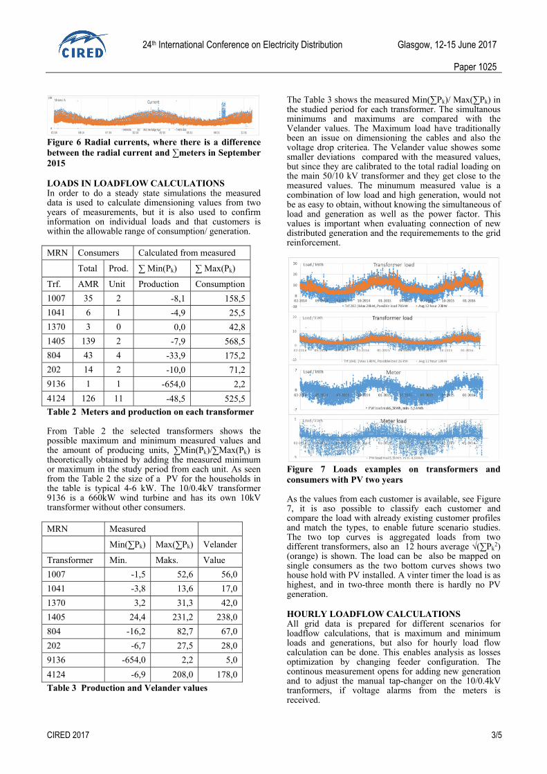
Figure 7 Loads examples on transformers and consumers with PV two years As the values from each customer is available, see Figure 7, it is aso possible to classify each customer and compare the load with already existing customer profiles and match the types, to enable future scenario studies. The two top curves is aggregated loads from two different transformers, also an 12 hours average √(∑Pk

2) (orange) is shown. The load can be also be mapped on single consumers as the two bottom curves shows two house hold with PV installed. A vinter timer the load is as highest, and in two-three month there is hardly no PV generation. HOURLY LOADFLOW CALCULATIONS All grid data is prepared for different scenarios for loadflow calculations, that is maximum and minimum loads and generations, but also for hourly load flow calculation can be done. This enables analysis as losses optimization by changing feeder configuration. The continous measurement opens for adding new generation and to adjust the manual tap-changer on the 10/0.4kV tranformers, if voltage alarms from the meters is received.


Paper 1025

CIRED 2017 4/5

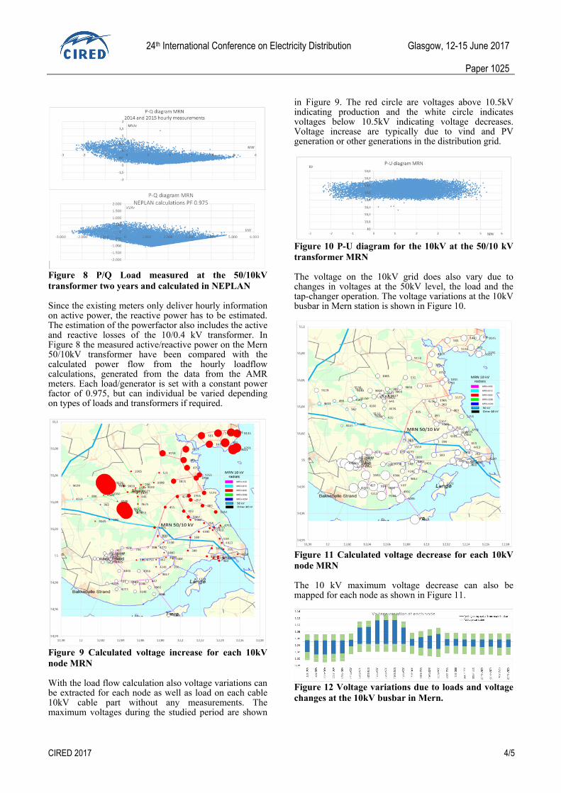
Figure 8 P/Q Load measured at the 50/10kV transformer two years and calculated in NEPLAN Since the existing meters only deliver hourly information on active power, the reactive power has to be estimated. The estimation of the powerfactor also includes the active and reactive losses of the 10/0.4 kV transformer. In Figure 8 the measured active/reactive power on the Mern 50/10kV transformer have been compared with the calculated power flow from the hourly loadflow calculations, generated from the data from the AMR meters. Each load/generator is set with a constant power factor of 0.975, but can individual be varied depending on types of loads and transformers if required.

Figure 9 Calculated voltage increase for each 10kV node MRN With the load flow calculation also voltage variations can be extracted for each node as well as load on each cable 10kV cable part without any measurements. The maximum voltages during the studied period are shown

in Figure 9. The red circle are voltages above 10.5kV indicating production and the white circle indicates voltages below 10.5kV indicating voltage decreases. Voltage increase are typically due to vind and PV generation or other generations in the distribution grid.

Figure 10 P-U diagram for the 10kV at the 50/10 kV transformer MRN The voltage on the 10kV grid does also vary due to changes in voltages at the 50kV level, the load and the tap-changer operation. The voltage variations at the 10kV busbar in Mern station is shown in Figure 10.

Figure 11 Calculated voltage decrease for each 10kV node MRN The 10 kV maximum voltage decrease can also be mapped for each node as shown in Figure 11.

Figure 12 Voltage variations due to loads and voltage changes at the 10kV busbar in Mern.


Paper 1025

CIRED 2017 5/5

By adding the voltage increase and voltage changes the total voltage variations range in the studied period at each 10 kV transformer can be mapped, as shown in Figure 12, where the voltage increase/decrease is shown as blue and voltage variation is shown as green. Losses in the 10 kV grid When optimizing the grid also the losses in the grid are of interest. Traditinally in Denmark the payments of losses is included in the fee depending of the load. The renewable generation does not pay this fee, because the claim is that the generation lower the losses. This is to some extent correct as long as the load on the line is less than 2 times the simulatanous generation, when this is not the case the losses will increase. In Denmark a compensation for the increased losses on pure radials to the distribution companies existes.

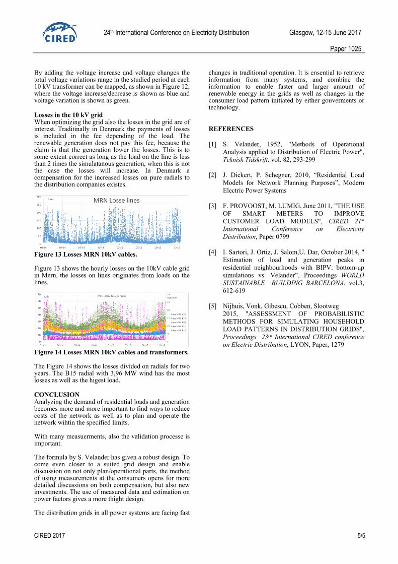
Figure 13 Losses MRN 10kV cables. Figure 13 shows the hourly losses on the 10kV cable grid in Mern, the losses on lines originates from loads on the lines.

Figure 14 Losses MRN 10kV cables and transformers. The Figure 14 shows the losses divided on radials for two years. The B15 radial with 3,96 MW wind has the most losses as well as the higest load. CONCLUSION Analyzing the demand of residential loads and generation becomes more and more important to find ways to reduce costs of the network as well as to plan and operate the network wihtin the specified limits. With many measuerments, also the validation processe is important. The formula by S. Velander has given a robust design. To come even closer to a suited grid design and enable discussion on not only plan/operational parts, the method of using measurements at the consumers opens for more detailed discussions on both compensation, but also new investments. The use of measured data and estimation on power factors gives a more thight design. The distribution grids in all power systems are facing fast

changes in traditional operation. It is ensential to retrieve information from many systems, and combine the information to enable faster and larger amount of renewable energy in the grids as well as changes in the consumer load pattern initiated by either gouverments or technology. REFERENCES [1] S. Velander, 1952, "Methods of Operational

Analysis applied to Distribution of Electric Power", Teknisk Tidskrift. vol. 82, 293-299

[2] J. Dickert, P. Schegner, 2010, “Residential Load

Models for Network Planning Purposes”, Modern Electric Power Systems

[3] F. PROVOOST, M. LUMIG, June 2011, "THE USE

OF SMART METERS TO IMPROVE CUSTOMER LOAD MODELS", CIRED 21st International Conference on Electricity Distribution, Paper 0799

[4] I. Sartori, J. Ortiz, J. Salom,U. Dar, October 2014, "

Estimation of load and generation peaks in residential neighbourhoods with BIPV: bottom-up simulations vs. Velander”, Proceedings WORLD SUSTAINABLE BUILDING BARCELONA, vol.3, 612-619

[5] Nijhuis, Vonk, Gibescu, Cobben, Slootweg

2015, "ASSESSMENT OF PROBABILISTIC METHODS FOR SIMULATING HOUSEHOLD LOAD PATTERNS IN DISTRIBUTION GRIDS", Proceedings 23rd International CIRED conference on Electric Distribution, LYON, Paper, 1279

grid planning by integrate customer...

Documents