grnsight: a web application and service for visualizing ... · models of small- to medium-scale...

GRNsight: a web application and service for visualizingmodels of small- to medium-scale gene regulatory networksKam D Dahlquist Corresp., 1 , John David N Dionisio 2 , Ben G Fitzpatrick 3 , Nicole A Anguiano 2 , AninditaVarshneya 1 , Britain J Southwick 2 , Mihir Samdarshi 1

1 Department of Biology, Loyola Marymount University, Los Angeles, California, United States2 Department of Electrical Engineering and Computer Science, Loyola Marymount University, Los Angeles, California, United States3 Department of Mathematics, Loyola Marymount University, Los Angeles, California, United States

Corresponding Author: Kam D DahlquistEmail address: [email protected]

GRNsight is a web application and service for visualizing models of gene regulatorynetworks (GRNs). A gene regulatory network consists of genes, transcription factors, andthe regulatory connections between them which govern the level of expression of mRNAand protein from genes. The original motivation came from our efforts to performparameter estimation and forward simulation of the dynamics of a differential equationsmodel of a small GRN with 21 nodes and 31 edges. We wanted a quick and easy way tovisualize the weight parameters from the model which represent the direction andmagnitude of the influence of a transcription factor on its target gene, so we createdGRNsight. GRNsight automatically lays out either an unweighted or weighted networkgraph based on an Excel spreadsheet containing an adjacency matrix where regulators arenamed in the columns and target genes in the rows, a Simple Interaction Format (SIF) textfile, or a GraphML XML file. When a user uploads an input file specifying an unweightednetwork, GRNsight automatically lays out the graph using black lines and pointedarrowheads. For a weighted network, GRNsight uses pointed and blunt arrowheads, andcolors the edges and adjusts their thicknesses based on the sign (positive for activation ornegative for repression) and magnitude of the weight parameter. GRNsight is written inJavaScript, with diagrams facilitated by D3.js, a data visualization library. Node.js and theExpress framework handle server-side functions. GRNsight’s diagrams are based on D3.js’sforce graph layout algorithm, which was then extensively customized to support thespecific needs of GRNs. Nodes are rectangular and support gene labels of up to 12characters. The edges are arcs, which become straight lines when the nodes are closetogether. Self-regulatory edges are indicated by a loop. When a user mouses over an edge,the numerical value of the weight parameter is displayed. Visualizations can be modifiedby sliders that adjust the force graph layout parameters and through manual nodedragging. GRNsight is best-suited for visualizing networks of fewer than 35 nodes and 70

PeerJ Preprints | https://doi.org/10.7287/peerj.preprints.2068v2 | CC BY 4.0 Open Access | rec: 18 Aug 2016, publ: 18 Aug 2016

edges, although it accepts networks of up to 75 nodes or 150 edges. GRNsight has generalapplicability for displaying any small, unweighted or weighted network with directed edgesfor systems biology or other application domains. GRNsight serves as an example offollowing and teaching best practices for scientific computing and complying with FAIRPrinciples, using an open and test-driven development model with rigorous documentationof requirements and issues on GitHub. An exhaustive unit testing framework using Mochaand the Chai assertion library consists of around 160 automated unit tests that examinenearly 530 test files to ensure that the program is running as expected. The GRNsightapplication (http://dondi.github.io/GRNsight/) and code(https://github.com/dondi/GRNsight) are available under the open source BSD license.


1 GRNsight: a web application and service for visualizing models of 2 small- to medium-scale gene regulatory networks

3 Kam D. Dahlquist1*, John David N. Dionisio2, Ben G. Fitzpatrick3, Nicole A. Anguiano2,

4 Anindita Varshneya1, Britain J. Southwick2, Mihir Samdarshi1

5 1Department of Biology, 2Department of Electrical Engineering and Computer Science,

6 3Department of Mathematics, Loyola Marymount University, 1 LMU Drive, Los Angeles, CA

7 90045 USA

8 *Corresponding author:

9 Kam D. Dahlquist

10 Department of Biology

11 Loyola Marymount University

12 1 LMU Drive, MS8888

13 Los Angeles, CA 90045 USA

14 E-mail: [email protected]

15 Tel: 1-310-338-7697

16 Link to web application: http://dondi.github.io/GRNsight/

17 Link to code repository: https://github.com/dondi/GRNsight


18 Abstract

19 GRNsight is a web application and service for visualizing models of gene regulatory

20 networks (GRNs). A gene regulatory network consists of genes, transcription factors, and the

21 regulatory connections between them which govern the level of expression of mRNA and protein

22 from genes. The original motivation came from our efforts to perform parameter estimation and

23 forward simulation of the dynamics of a differential equations model of a small GRN with 21

24 nodes and 31 edges. We wanted a quick and easy way to visualize the weight parameters from

25 the model which represent the direction and magnitude of the influence of a transcription factor

26 on its target gene, so we created GRNsight. GRNsight automatically lays out either an

27 unweighted or weighted network graph based on an Excel spreadsheet containing an adjacency

28 matrix where regulators are named in the columns and target genes in the rows, a Simple

29 Interaction Format (SIF) text file, or a GraphML XML file. When a user uploads an input file

30 specifying an unweighted network, GRNsight automatically lays out the graph using black lines

31 and pointed arrowheads. For a weighted network, GRNsight uses pointed and blunt arrowheads,

32 and colors the edges and adjusts their thicknesses based on the sign (positive for activation or

33 negative for repression) and magnitude of the weight parameter. GRNsight is written in

34 JavaScript, with diagrams facilitated by D3.js, a data visualization library. Node.js and the

35 Express framework handle server-side functions. GRNsight’s diagrams are based on D3.js’s

36 force graph layout algorithm, which was then extensively customized to support the specific

37 needs of GRNs. Nodes are rectangular and support gene labels of up to 12 characters. The edges

38 are arcs, which become straight lines when the nodes are close together. Self-regulatory edges

39 are indicated by a loop. When a user mouses over an edge, the numerical value of the weight

40 parameter is displayed. Visualizations can be modified by sliders that adjust the force graph


41 layout parameters and through manual node dragging. GRNsight is best-suited for visualizing

42 networks of fewer than 35 nodes and 70 edges, although it accepts networks of up to 75 nodes or

43 150 edges. GRNsight has general applicability for displaying any small, unweighted or weighted

44 network with directed edges for systems biology or other application domains. GRNsight serves

45 as an example of following and teaching best practices for scientific computing and complying

46 with FAIR Principles, using an open and test-driven development model with rigorous

47 documentation of requirements and issues on GitHub. An exhaustive unit testing framework

48 using Mocha and the Chai assertion library consists of around 160 automated unit tests that

49 examine nearly 530 test files to ensure that the program is running as expected. The GRNsight

50 application (http://dondi.github.io/GRNsight/) and code (https://github.com/dondi/GRNsight) are

51 available under the open source BSD license.


52 Introduction

53 GRNsight is a web application and service for visualizing models of small- to medium-

54 scale gene regulatory networks (GRNs). A gene regulatory network consists of genes,

55 transcription factors, and the regulatory connections between them which govern the level of

56 expression of mRNA and protein from genes. Our group has developed a MATLAB program to

57 perform parameter estimation and forward simulation of the dynamics of an ordinary differential

58 equations model of a medium-scale GRN with 21 nodes and 31 edges (Dahlquist et al., 2015;

59 http://kdahlquist.github.io/GRNmap/). GRNmap accepts a Microsoft Excel workbook as input,

60 with multiple worksheets specifying the different types of data needed to run the model. For

61 compactness, the GRN itself is specified by a worksheet that contains an adjacency matrix where

62 regulators are named in the columns and target genes in the rows. Each cell in the matrix

63 contains a “0” if there is no regulatory relationship between the regulator and target, or a “1” if

64 there is a regulatory relationship between them. The GRNmap program then outputs the

65 estimated weight parameters in a new worksheet containing an adjacency matrix where the “1’s”

66 are replaced with a real number that is the weight parameter, representing the direction (positive

67 for activation or negative for repression) and magnitude of the influence of the transcription

68 factor on its target gene (Dahlquist et al., 2015). Although MATLAB has graph layout

69 capabilities, we wanted a way for novice and experienced biologists alike to quickly and easily

70 view the unweighted and weighted network graphs corresponding to the matrix without having

71 to create or modify MATLAB code. Given that our user base included students in courses using

72 university computer labs where the installation and maintenance of software is subject to

73 logistical considerations sometimes beyond our control, we enumerated the following

74 requirements for a potential visualization tool. The tool should:


75 1. Exist as a web application without the need to download and install specialized software;

76 2. Be simple and intuitive to use;

77 3. Accept an input file in Microsoft Excel format (.xlsx);

78 4. Read a weighted or unweighted adjacency matrix where the regulatory transcription

79 factors are in columns and the target genes are in rows;

80 5. Automatically lay out and display small- to medium-scale, unweighted and weighted,

81 directed network graphs in a way that is familiar to biologists and adds value to the

82 interpretation of the modeling results.

83 Having established the broad technical requirements to which we were seeking a

84 solution, the first task was to determine if software already existed that could fulfill our needs. A

85 review by Pavlopoulos et al., published in 2015, describes the types, trends, and usage of

86 visualization tools available for genomics and systems biology. Their list of 47 tools for network

87 analysis is representative of what was available to us at our project inception in January 2014

88 (given the caveat that the list itself is a moving target with some tools dropping out, new ones

89 being added, and others evolving in their functions). With such a large number of tools

90 available, it would be reasonable to expect that one already existed that could fulfill our needs.

91 However, our use case was narrow, and the tools we investigated out of this diverse set each had

92 properties that limited their use for us. With regard to our first requirement, out of the 47 tools,

93 29 are stand-alone applications, requiring installation, versus 18 web applications. With respect

94 to our second requirement, the more complex software packages out of the set have a steep

95 learning curve. Our third and fourth requirements specify data types. Some packages were

96 hardcoded for a different type of network than a GRN (e.g., metabolic or signaling pathways,

97 protein-protein interaction networks) or retrieved data exclusively from a backend database, not


98 allowing user-supplied data. None at the time would readily accept an adjacency matrix with the

99 GRNmap specifications as input without some manipulation of the data format. Finally, with

100 respect to the last requirement, the core functionality, some packages were designed for

101 visualization and analysis of much larger networks than the ones in which we were interested or

102 did not have the ability to display directed, weighted graphs.

103 As an illustration of this, Pavlopoulos et al. (2015) showed that the open source software,

104 Cytoscape (Shannon et al., 2003; Smoot et al., 2011) had the highest citation count in the Scopus

105 database, as it is widely recognized as the “best-in-class” tool for viewing and analyzing large

106 networks for systems biology research. However, while Cytoscape is flexible in terms of what

107 types of network representations it accepts as input (SIF, NNF, GML, XGMML, SBML,

108 BioPAX, PSI-MI, GraphML, cf.

109 http://manual.cytoscape.org/en/latest/Supported_Network_File_Formats.html#supported-

110 network-file-formats), its basic “unformatted table files” format expects the network to be

111 represented in a list of pairwise interactions between two nodes instead of as an adjacency

112 matrix, requiring a GRNmap user to convert the file external to the program. Furthermore,

113 Cytoscape must be installed on a user’s computer. Finally, because it is powerful and has a lot of

114 features, there is a somewhat steep learning curve before a novice user can begin to visualize

115 networks. Multiple settings must be learned and selected to generate a display that properly fits

116 a use case; it is not possible to just “load into Cytoscape and go.” Another open source

117 application, Gephi (Bastian, Heymann, and Jacomy, 2009), is a general graph visualization tool

118 that does accept an adjacency matrix in .csv format (among a wide range of supported formats,

119 cf. https://gephi.org/users/supported-graph-formats/csv-format/), but again requires download

120 and installation of the software and has a complex feature set. Because GRNmap itself is


121 complex software targeted both at experienced biology investigators and novice undergraduate

122 users in a Biomathematical Modeling course, we wanted to limit the need to install and learn

123 additional visualization software. Reducing the cognitive load required for using the software

124 would allow users to focus their attention on understanding the biological results of the model.

125 After this exploration, we decided to create our own software solution that we could

126 exactly tailor to our specifications. Following the philosophy of “do one thing well”

127 (http://onethingwell.org/post/457050307/about-one-thing-well), we wanted to prioritize

128 rendering small- to medium-scale gene regulatory networks both easily and well. It was more

129 important for us to create a tool that is specifically tailored to the visualization of these sized

130 GRNs, and not every possible graph from every possible application domain. Similarly, we

131 wanted to pass data seamlessly from GRNmap to GRNsight, while bearing in mind that we

132 should adopt practices that would also make our tool useful to users outside our own group.

133 Finally, we wanted to minimize any startup, onboarding, or overhead time, which necessitated

134 also enumerating a set of process requirements that would lead us to our goal. Our project

135 should:

136 Follow best practices for open software development in bioinformatics, including:

137 reusing code, releasing early and often to a public repository, tracking requirements,

138 issues, and bugs, performing unit-tests, and providing both code and user documentation

139 (Schultheiss, 2011; Prlic and Procter, 2012; Wilson et al., 2014);

140 Leverage the expertise of the faculty and undergraduate student development team

141 members and be responsive to our GRNmap customers (i.e., eat our own dog food);


142 Balance the needs of fulfilling our own use case with developing a tool of wider

143 applicability to the scientific community during a development cycle that ebbs and flows

144 with the pressures of the academic calendar.

145 GRNsight both fulfills our stated product requirements and serves as a model for best practices

146 for software development in bioinformatics as discussed in the sections below.

147 Materials and Methods

148 Input Data

149 GRNsight automatically lays out the network graph specified by an adjacency matrix

150 contained within a worksheet named “network” or “network_optimized_weights” in a Microsoft

151 Excel workbook (.xlsx). It was designed to accept workbooks seamlessly from the MATLAB

152 gene regulatory network modeling program, GRNmap; however, the expected input format is

153 general and is not dependent on GRNmap. Detailed documentation for the expected input file

154 format is found on the GRNsight Documentation page:

155 http://dondi.github.io/GRNsight/documentation.html.

156 GRNsight can automatically lay out either an unweighted or weighted network graph

157 specified by an adjacency matrix where regulators are named in the columns and target genes in

158 the rows. Note that regulators (regulatory transcription factors) are themselves encoded by genes

159 and will be referred to as such. The adjacency matrix can be either symmetric (with the exact

160 same genes named in both the columns and rows) or asymmetric (additional genes in either the

161 columns or rows or both). For an unweighted network, each cell in the matrix should contain a

162 “0” if there is no regulatory relationship between the regulator and target, or a “1” if there is a


163 regulatory relationship between them (Fig. 1). In a weighted network, the “1’s” are replaced

164 with a real number that is the weight parameter (Fig. 2). Positive weights indicate activation of

165 the target gene by the regulator, and negative weights indicate repression of the target gene by

166 the regulator.

167 After having implemented the core functionality of seamlessly reading GRNmap-

168 generated Excel workbooks, we recently extended the ability of GRNsight to read other

169 commonly used network data formats to increase the interoperability of GRNsight with other

170 network analysis and visualization software. GRNsight can import and display Simple

171 Interaction Format (SIF, .sif,

172 http://manual.cytoscape.org/en/latest/Supported_Network_File_Formats.html#sif-format) and

173 GraphML (.graphml; Brandes et al., 2001; http://graphml.graphdrawing.org/) files and export

174 network data in those two formats (see the GRNsight Documentation page for details of the

175 implementation at http://dondi.github.io/GRNsight/documentation.html).

176 GRNsight is designed to visualize small- to medium-scale GRNs, not the entire gene

177 regulatory network for an organism. The bounding box for display of the graph has a fixed size.

178 Currently, it is recommended that the user upload networks with no more than 35 unique genes

179 (nodes) or 70 edges. A warning is given upon upload of a network with 50-74 nodes or 71-99

180 edges, although the network graph will still display. If the user attempts to upload a network of

181 75 or more nodes or 100 or more edges, the graph does not display, and an error message will be

182 returned.


183 Architecture

184 GRNsight has a service-oriented architecture, consisting of separate server and web client

185 components (Fig. 3). The server provides a web API (application programming interface) that

186 accepts a Microsoft Excel workbook (.xlsx) file via a POST request and converts it into a

187 corresponding JSON (JavaScript Object Notation) representation. Conversion is accomplished

188 by first parsing the .xlsx file using the node-xlsx library (https://github.com/mgcrea/node-xlsx)

189 then mapping the translated worksheet cells into JSON. It also provides demonstration graphs

190 already in this JSON format, without requiring a spreadsheet upload. The web client provides a

191 graphical user interface for visualizing the JSON graphs provided by the server, whether the

192 graphs are parsed from uploaded Excel workbooks or provided directly by the server’s demos.

193 As an additional layer of customization, the graphical interface provided by the web client can be

194 embedded in any web page using the standard iframe element. This is the mechanism used in

195 deploying the production and beta versions of the software on https://dondi.github.io/GRNsight.

196 Figure 3 illustrates this architecture and the interactions of the components. Documentation for

197 how GRNsight is specifically deployed, including autonomous production and beta versions, can

198 be found on the GRNsight wiki (https://github.com/dondi/GRNsight/wiki/Server-Setup).

199 GRNsight is an open source project and is itself built using other open source software.

200 Server-side components are implemented with Node.js and the Express framework (Brown,

201 2014). Graph visualization is facilitated by the Data-Driven Documents JavaScript library

202 (D3.js; Bostock, Ogievetsky, and Heer, 2011). D3.js provides data mapping and layout routines

203 which GRNsight heavily customizes in order to achieve the desired graph visualization. The

204 resulting graph is a Scalable Vector Graphics (SVG) drawing in which D3.js maps gene objects

205 from the JSON representation provided by the web API server onto labeled rectangles. Edge


206 weights are mapped into Bezier curves. The resulting graph is interactive, initially using D3.js’s

207 force graph layout algorithm to automatically determine the positions of the gene rectangles.

208 The user can then drag the rectangles to improve the graph’s layout. Customizations to the graph

209 display are described further in the next section.

210 As noted in the Introduction, we decided to create our own GRNsight software instead of

211 utilizing prior existing network visualization packages, like Cytoscape (Shannon et al., 2003;

212 Smoot et al., 2011). However, in keeping with open source development practices, we did

213 leverage other pre-existing code as described above. Besides D3.js, Cytoscape.js (Franz et al.,

214 2016) has been developed as an open source network visualization engine. The BioJS registry

215 (Yachdav et al., 2015) also lists a dozen components tagged with the keyword “network.” The

216 choice of D3.js as the visualization engine was made simply to leverage the expertise of one of

217 the co-authors who was already familiar with the D3.js library in order to minimize the startup,

218 onboarding, and overhead time for the project, which initially served as a semester-long capstone

219 experience for one of the undergraduate co-authors.

220 Graph Customizations

221 GRNsight’s diagrams are based on D3.js’s force graph layout algorithm (Bostock,

222 Ogievetsky, and Heer, 2011), which was then extensively customized to support the specific

223 needs of biologists for GRN visualization. D3.js’s baseline force graph implementation had

224 round, unlabeled nodes and undirected, straight-line edges. The following customizations were

225 made for the nodes: (a) the nodes were made rectangular; (b) a label of up to 12 characters was

226 added; (c) node size was varied, depending on the size of the label.


227 Customizations were also made for the edges. Instead of undirected, straight line

228 segments, the edges display as directed edges. They are implemented as Bezier curves that

229 straighten when nodes are close together and curve when nodes are far apart. A special case was

230 added to form a looping edge if a node regulated itself. When an unweighted adjacency matrix is

231 uploaded, all edges are displayed as black with pointed arrowheads. When a weighted adjacency

232 matrix is uploaded, edges are further customized based on the sign and magnitude of the weight

233 parameter. As is common practice in biological pathway diagrams (Gostner et al., 2014),

234 activation (for positive weights) is represented by pointed arrowheads, and repression (for

235 negative weights) is represented by a blunt end marker, i.e., a line segment perpendicular to the

236 edge. The thickness of the edge also varies based on the magnitude of the absolute value of the

237 weight. Larger magnitudes have thicker edges and smaller magnitudes have thinner edges. The

238 way that GRNsight determines the edge thickness is as follows: GRNsight divides all weight

239 values by the absolute value of the maximum weight in the adjacency matrix to normalize all the

240 values to between zero and 1. GRNsight then adjusts the thickness of the lines to vary

241 continuously from the minimum thickness (for normalized weights near zero) to maximum

242 thickness (normalized weight of 1). The color of the edge also imparts information about the

243 regulatory relationship. Edges with positive normalized weight values from 0.05 to 1 are colored

244 magenta; edges with negative normalized weight values from -0.05 to -1 are colored cyan. Edges

245 with normalized weight values between -0.05 and 0.05 are colored grey to emphasize that their

246 normalized magnitude is near zero and that they have a weak influence on the target gene. When

247 a user mouses over an edge, the numerical value of the weight parameter is displayed. When the

248 user drags nodes to customize his or her view of the network, edges adapt their anchor points to

249 the movements of the nodes.


250 User Interface

251 The GRNsight user interface includes a menu/status bar and sliders that adjust D3.js’s

252 force graph layout parameters. Figure 4 provides an annotated screenshot of the user interface,

253 highlighting its primary features. Users can move force graph parameter sliders to refine the

254 automated visualization. Nodes have a charge, which repels or attracts other nodes. The charge

255 distance determines at what range a node’s charge will affect other nodes. The link distance

256 determines the minimum distance maintained between nodes. Gravity determines the strength of

257 the force drawing the nodes to the center of the graph. Sliders can be locked to prevent changes

258 and also reset to default values. Graph visualizations can also be modified through manual node

259 dragging. Design decisions for the user interface were driven by applicable interaction design

260 guidelines and principles (Nielsen, 1993; Shneiderman et al., 2016; Norman, 2013) in alignment

261 with the mental model and expectations of the target user base, consisting primarily of biologists,

262 both novice and experienced.

263 Test-driven Development

264 GRNsight follows an open development model with rigorous documentation of

265 requirements and issues on GitHub. We have implemented an exhaustive unit testing framework

266 using Mocha (https://mochajs.org) and the Chai assertion library (http://chaijs.com) to perform

267 test-driven development where unit tests are written before new functionality is coded (Martin,

268 2008). This framework consists of around 160 automated unit tests that examine nearly 530 test

269 files to ensure that the program is running as expected. Table 1 shows the test suite’s coverage

270 report, as generated by Istanbul (https://gotwarlost.github.io/istanbul/).


271 Error and warning messages have a three-part framework that informs the user what

272 happened, the source of the problem, and possible solutions. This structure follows the alert

273 elements recommended by user interface guideline documents such as the OS X Human

274 Interface Guidelines

275 (https://developer.apple.com/library/mac/documentation/UserExperience/Conceptual/OSXHIGui

276 delines/WindowAlerts.html). For example, GRNsight returns an error when the spreadsheet is

277 formatted incorrectly or the maximum number of nodes or edges is exceeded.

278 Availability

279 GRNsight (currently version 1.18.1) is available at http://dondi.github.io/GRNsight/and is

280 compatible with Google Chrome version 43.0.2357.65 or higher and Mozilla Firefox version

281 38.0.1 or higher on the Windows 7 and Mac OS X operating systems. The website is free and

282 open to all users, and there is no login requirement. Website content is available under the

283 Creative Commons Attribution Non-Commercial Share Alike 3.0 Unported License. GRNsight

284 code is available under the open source BSD license from our GitHub repository

285 https://github.com/dondi/GRNsight. Every user’s submitted data are private and not viewable by

286 anyone other than the user. Uploaded data reside as temporary files and are deleted from the

287 GRNsight server during standard operating system file cleanup procedures. A Google Analytics

288 page view counter was implemented on 18 September 2014, and a file upload counter was added

289 on 13 April 2015. From these start dates and as of 12 August 2016, the GRNsight home page

290 has been accessed 2349 times, and 1652 files have been uploaded and viewed with GRNsight. Of

291 these 1652 files, an estimated 148 were uploaded by users outside of our group.


292 Results and Discussion

293 We have successfully implemented GRNsight, a web application and service for

294 visualizing small- to medium-scale gene regulatory networks, fulfilling our five requirements:

295 1. It exists as a web application without the need to download and install specialized

296 software;

297 2. It is simple and intuitive to use;

298 3. It accepts an input file in Microsoft Excel format (.xlsx), as well as SIF (.sif) and

299 GraphML (.graphml);

300 4. It reads a weighted or unweighted adjacency matrix where the regulatory transcription

301 factors are in columns and the target genes are in rows (Excel format-only);

302 5. It automatically lays out and displays small- to medium-scale, unweighted and weighted,

303 directed network graphs in a way that is familiar to biologists, adding value to the

304 interpretation of the modeling results.

305 GRNsight Facilitates Interpretation of GRN Model Results

306 GRNsight facilitates the biological interpretation of unweighted and weighted gene

307 regulatory network graphs. Our discussion focuses on two of the demonstration files provided in

308 the user interface, Demo #3: Unweighted GRN (21 genes, 31 edges) and Demo #4: Weighted

309 GRN (21 genes, 31 edges, Schade et al. 2004 data). These two files describe gene regulatory

310 networks from budding yeast, Saccharomyces cerevisiae, correspond to supplementary data

311 published by Dahlquist et al. (2015), and when displayed by GRNsight, represent interactive

312 versions of Figures 1 and 8 of that paper, respectively.


313 Figure 5 gives a side-by-side view of the same adjacency matrices laid out by GRNsight

314 and by hand. Figures 5A, 5B, and 5C are derived from Demo #3: Unweighted GRN (21 genes,

315 31 edges), and Figures 5D, 5E, and 5F are derived from Demo #4: Weighted GRN (21 genes, 31

316 edges, Schade et al. 2004 data). Figures 5A and 5D show examples of the automatic layout

317 performed by GRNsight. Figures 5C and 5F show the same adjacency matrices laid out by hand

318 in Adobe Illustrator, corresponding to Figure 1 and Figure 8 of Dahlquist et al. (2015),

319 respectively. Figures 5B and 5E started with the automatic layout from GRNsight and then were

320 manually manipulated from within GRNsight to lay them out similarly to Figures 5C and 5F,

321 respectively. The use of GRNsight represents a substantial time savings compared to creating the

322 same figures entirely by hand and allows the user to try multiple arrangements of the nodes

323 quickly and easily. Note that this type of “by hand” manipulation of graphs is most useful for

324 small- to medium-scale networks, the kind that GRNsight is designed to display, and would not

325 be appropriate for large networks.

326 Viewing the unweighted network (Fig. 5A, B, C) allows one to make observations about

327 the network structure (Dahlquist et al., 2015). For example, YAP6 has the highest in-degree,

328 being regulated by six other transcription factors. RAP1 has the highest out-degree of five,

329 regulating four other transcription factors and itself. Four genes, AFT1, NRG1, RAP1, and

330 YAP6, regulate themselves. Many of the transcription factors are involved in regulatory chains,

331 with the longest including five nodes originating at SKN7 or ACE2. There are several other 4-

332 node chains that originate at CIN5, MAC1, PHD1, SKN7, and YAP1. Finally, there are two

333 rather complex feedforward motifs involving CIN5, ROX1, and YAP6 and SKN7, YAP1, and

334 ROX1 (Dahlquist et al., 2015).


335 The networks with colored edges (Fig. 5D, E, F) display the results of a mathematical

336 model, where the expression levels of the individual transcription factors were modeled using

337 mass balance ordinary differential equations with a sigmoidal production function and linear

338 degradation (Dahlquist et al., 2015). Each equation in the model included a production rate, a

339 degradation rate, weights that denote the magnitude and type of influence of the connected

340 transcription factors (activation or repression), and a threshold of expression. The differential

341 equation model was fit to published yeast cold shock microarray data from Schade et al. (2004)

342 using a penalized nonlinear least squares approach. The visualization produced by GRNsight is

343 displaying the results of the optimized weight parameters. Positive weights > 0 represent an

344 activation relationship and are shown by pointed arrowheads. One example is that CIN5

345 activates the expression of MSN1. Negative weights < 0 represent a repression relationship and

346 are shown by a blunt arrowhead. One example is that ABF1 represses the expression of MSN1.

347 The thicknesses of the edges also vary based on the magnitude of the absolute value of the

348 weight, with larger magnitudes having thicker edges and smaller magnitudes having thinner

349 edges. In Figures 5D, E, and F, the edge corresponding to the repression of the expression of

350 MSN1 by ABF1 stands out as the thickest because the absolute value of its weight parameter (-

351 2.97) has the largest magnitude out of all the weights (Dahlquist et al., 2015). It is noticeable

352 that none of the edges that represent activation are as thick as the ABF1-to-MSN1 edge; only

353 RAP1-to-RPH1 and HAL9-to-MSN4 are close with weights of 1.50 and 1.43, respectively.

354 The color of the edge also imparts information about the regulatory relationship. Edges

355 with positive normalized weight values from 0.05 to 1 are colored magenta (10 edges in this

356 example); edges with negative normalized weight values from -0.05 to -1 are colored cyan (16

357 edges in this example). Edges with normalized weight values between -0.05 and 0.05 are colored


358 grey to indicate that their normalized magnitude is near zero and that they have a weak influence

359 on the target gene (5 edges in this example). The grey color de-emphasizes the weak

360 relationships to the eye, thus emphasizing the stronger colored relationships.

361 Because of this visualization of the weight parameters, one can make some interesting

362 observations about the behavior of the network (Dahlquist et al., 2015). Taking the arrowhead

363 type, thickness, and color into consideration, one can, by visual inspection, group edges by type

364 and relative influence into four activation and four repression bins. RAP1-to-RPH1, HAL9-to-

365 MSN4, and NRG1 to itself have the strongest activation relationships, followed by CIN5-to-

366 MSN1, followed by NRG1-to-YAP6, MSN4-to-FHL1, SKN7-to ROX1 and PHD1-to-MSN4,

367 followed by ABF1-to-FHL1 as the weakest of the activation relationships. The aforementioned

368 ABF1-to-MSN1 edge has the strongest repression relationship, followed by ACE2-to-YAP1,

369 RAP1-to-HSF1, CIN5-to-ROX1, AFT1 to itself, and RAP1 to itself, followed by ROX1-to-

370 YAP6, PHD1-to-CUP9, CIN5-to-YAP6, YAP6-to-ROX1, YAP1-to-ROX1, SKN7-to-YAP1,

371 RAP1-to-AFT1, and YAP6 to itself, followed by MAC1-to-CUP9 and SKN7-to-NRG1 as the

372 weakest of the repression relationships. These rankings could have been obtained, of course, by

373 sorting the numerical values of the edges in a table, but it is notable that these groupings can also

374 be picked out by eye and then put into the context of the other network connections.

375 Because the five weakest connections, CUP9-to-YAP6, REB1-to-GTS1, YAP6-to-CIN5,

376 YAP1-to-YAP6, and HSF1-to-REB1, colored grey, are de-emphasized in the visual display, a

377 different interpretation of the network structure can be made as compared to the unweighted

378 network (Fig. 5E and F versus 5B and C). In most cases, nodes in a regulatory chain “drop out”

379 visually “breaking” the chain. For example, in the four-node chain beginning with RAP1-to-

380 HSF1, the last two nodes, REB1 and GTS1, are only weakly connected. In the five-node chains


381 beginning with SKN7-to-YAP1 or ACE2-to-YAP1, and the four-node chains beginning with

382 MAC1-to-CUP9 or PHD1-to-CUP9, the nodes connected to YAP6 drop out (YAP1-to-YAP6,

383 YAP6-to-CIN5, and CUP9-YAP6). This suggests that regulatory chains may only be effective

384 to a depth of two levels, and that while longer chains are theoretically possible, given the

385 network connections, they have a negligible effect on the dynamics of expression of downstream

386 genes.

387 Another interpretation of the network structure that is highlighted by the weighted display

388 is that the 21-gene network can be divided into two smaller subnetworks by removing the two

389 edges CUP9-to-YAP6 (grey) and ABF1-to-FHL1 (thin magenta, weakly activating). While this

390 could also be observed in the unweighted network, the application of the weight information,

391 showing only thin connections between the two subnetworks, suggests that they could function

392 relatively independently. Finally, the unweighted display showed two complex feedforward

393 motifs involving CIN5, ROX1, and YAP6 and SKN7, YAP1, and ROX1. The weighted display

394 reveals that the complexity of the connections is reduced because the weak YAP1-to-YAP6 and

395 YAP6-to-CIN5 edges drop out. Furthermore, the display shows that the modeling predicts that

396 the three-node CIN5-ROX1-YAP6 motif is an incoherent type 2 feedforward loop, while the

397 SKN7-YAP1-ROX1 motif is a coherent type 4 feedforward loop, neither of which is found very

398 commonly in Escherichia coli nor S. cerevisiae gene regulatory networks (Alon, 2007). The

399 modeling combined with the display suggests that further investigation is warranted: either these

400 two rare types of feedforward loops are important to the dynamics of this particular GRN, or the

401 network structure is incorrect. In either case, future lines of experimental investigation are

402 suggested to the user.


403 When examining individual genes in the network, one can see that the expression of

404 several genes is controlled by a balance of activation and repression by different regulators. For

405 example, the expression of MSN1 is strongly activated by CIN5, but even more strongly

406 repressed by ABF1. The expression of ROX1 is weakly activated by SKN7 and weakly

407 repressed by YAP1, CIN5, and YAP6. The expression of YAP6 is weakly activated by NRG1,

408 but weakly repressed by itself, CIN5, and ROX1. Furthermore, some transcription factors act

409 both as activators of some targets and repressors of other targets. For example, RAP1 activates

410 the expression of MSN4 and RPH1, but represses the expression of AFT1, HSF1, and itself.

411 PHD1, ABF1, CIN5, and SKN7 also both activate and repress their different target genes in the

412 network. For each of these regulators, there is experimental evidence to support their opposite

413 effects on gene expression, although not necessarily for these particular target genes (RAP1:

414 Shore and Nasmyth, 1987; PHD1: Borneman et al. 2006, ABF1: Buchman and Kornberg, 1990

415 and Miyake et al., 2004; CIN5 and SKN7: Ni et al., 2009). Except for CIN5, what these genes

416 have in common is that they themselves have no inputs in the network. The remaining no-input

417 genes (ACE2, MAC1, and HAL9) have only one outgoing edge in this network. Because these

418 genes have no inputs and, in some sense, have been artificially disconnected from the larger

419 GRN of the cell, one must not overinterpret the results of the modeling for these genes.

420 Thus, GRNsight enables one to interpret the weight parameters more easily than one

421 could from the adjacency matrix alone. Visual inspection has long been recognized by experts

422 such as Tufte (1983) and Card, Mackinlay, and Shneiderman (1999) as distinct from other forms

423 of purely numeric, computational, or algorithmic data analysis, and as the preceding discussion

424 highlights, it is this potential that can be derived specifically by visual inspection that is enabled

425 by GRNsight. Card, Mackinlay, and Shneiderman (1999) have identified six major ways,


426 documented in earlier literature and empirical studies, by which information visualization

427 amplifies cognition. Tufte’s seminal book The Visual Display of Quantitative Information

428 (1983) perhaps states it best: “Graphics reveal data. Indeed graphics can be more precise and

429 revealing than conventional statistical computations.”

430 Note that the nodes in Figure 5F are also colored in the style of GenMAPP 2 (Salomonis

431 et al., 2007), based on the time course of expression of that gene in the Schade et al. (2004)

432 microarray data (stripes from left to right, 10, 30, and 120 minutes of cold shock, with magenta

433 representing a significant increase in expression relative to the control at time 0, cyan

434 representing a significant decrease in expression relative to the control, and grey representing no

435 significant change in expression relative to the control). This feature has not yet been

436 implemented in GRNsight, but is currently under development for Version 2.

437 These observations made by direct inspection of the GRNsight graph are for a relatively

438 small GRN of 21 genes and 31 edges and become more difficult as nodes and edges are added.

439 For much larger networks, a more powerful graph analysis tool such as Cytoscape (Shannon et

440 al., 2003; Smoot et al., 2011) or Gephi (Bastian, Heymann, and Jacomy, 2009) is warranted.

441 However, for small networks in the range of 15-35 nodes, GRNsight fulfills a need to quickly

442 and easily view and manipulate them. The GRN modeled in Dahlquist et al. (2015) and

443 displayed in Figure 5 was derived by hand from the Lee et al. (2002) and Harbison et al. (2004)

444 datasets generated by chromatin immunoprecipitation followed by microarray analysis. We have

445 also used GRNsight to display GRNs derived from the YEASTRACT database (Teixeira et al.,

446 2014), whose own display tool is static, displaying regulators and targets in two rows.

447 Instructions for viewing YEASTRACT-derived GRNs can be found on the GRNsight

448 documentation page.


449 While GRNsight was designed originally for viewing gene regulatory networks, it is not

450 specific for any particular species, nor for that kind of data. As long as the text strings used as

451 identifiers for the “regulators” and “targets” match, it can be used to visualize any small,

452 unweighted or weighted network with directed edges for systems biology or other application

453 domains.

454 GRNsight Development Follows Best Practices for Scientific Computing and FAIR Data 455 Principles

456 Veretnik, Fink, and Bourne (2008) lament and Schultheiss et al. (2011) document that

457 some computational biology resources, especially web servers, lack persistence and usability,

458 leading to an inability to reproduce results. With that in mind, we have consciously followed

459 best practices for open development (Prlic and Procter, 2012), scientific computing (Wilson et

460 al., 2014), providing a web resource (Schultheiss, 2011), and FAIR data (Wilkinson et al., 2016),

461 simultaneously following and teaching these practices to the primary developers who were all

462 undergraduates. Each of these practices relates to each other, supporting reproducible research.

463 Open Development and Long-term Persistence

464 As noted in our process requirements in the Introduction, we have followed an open

465 development model since the project’s inception in January 2014, with our code available under

466 the open source BSD license at the public GitHub repository, where we “release early, release

467 often” (Torvalds in Raymond, 1999) and also track requirements, issues, and bugs. Indeed, our

468 project stands on the shoulders of other open source tools. Our unit-testing framework provides

469 confidence that the code works as expected. Detailed documentation for users (web page) and

470 developers (wiki) are provided. Demo data are also provided so users have both an example of

471 how to format input files and can see how the software should perform. As noted by Prlic and


472 Procter (2012), open development practices have a positive impact on the long-term

473 sustainability of a project. Furthermore, Schultheiss et al. (2011) describe twelve qualities for

474 evaluating web services that sum to a Long-Term-Score, which correlates with persistence of the

475 web service. GRNsight complies with all twelve requirements, providing: a stable web address

476 (using the github.io domain to host the website and Amazon Cloud Services to host the server

477 help to ensure long-term availability), version information, hosting country and institution, last

478 updated date, contact information, high usability, no registration requirement, no download

479 required, example data, fair testing possibility (both with demonstration Excel workbooks and

480 standard SIF and GraphML file types), and a functional service.

481 We are committed to continue development of the GRNsight resource, fixing bugs and

482 improving the software by adding features. The lead authors (Dahlquist, Dionisio, and

483 Fitzpatrick) are all tenured faculty, overseeing the design, code, testing, and documentation of

484 GRNsight and providing continuity to the project. Together we have mentored the

485 undergraduates (Anguiano, Varshneya, Southwick, and Samdarshi) who had primary

486 responsibility for coding, testing, and documentation, while also being full partners in the design

487 of the software. A pipeline has been established for onboarding new members to the project,

488 also providing continuity. Lawlor and Walsh (2015) detail some of the same issues of reliability

489 and reproducibility in bioinformatics software referred to by Wilson et al. (2014). Lawlor and

490 Walsh (2015) conclude that the ideal way to bring software engineering values into

491 bioinformatics research projects is to establish separate specialists in bioinformatics engineering.

492 We disagree. Through GRNsight, we have shown how best practices can be taught to

493 undergraduates concomitant with training in bioinformatics, as we have shown previously with

494 Master’s level students (Dionisio and Dahlquist, 2008).


495 FAIR Data Principles

496 The FAIR Guiding Principles for scientific data and stewardship state that data should be

497 Findable, Accessible, Interoperable, and Reusable by both humans and machines (Wilkinson et

498 al., 2016), with “data” loosely construed as any scholarly digital research object, including

499 software. As scientific software that interacts with data, the FAIR principles can apply to both

500 the GRNsight application and the network data it is used to visualize. Thus, we evaluate the

501 GRNsight project in terms of its “FAIRness” below.

502 Findable

503 The Findable principle states that metadata and data should have a globally unique and

504 persistent identifier, and that metadata and data should be registered or indexed in a searchable

505 resource (Wilkinson et al., 2016). In terms of software, the identifier is the name and version.

506 Because we utilize the GitHub release mechanism, GRNsight code is tagged with a version

507 (currently v1.18.1) and each version is available from the release page

508 (https://github.com/dondi/GRNsight/releases). We have registered GRNsight with well-known

509 bioinformatics tools registries: the BioJS Repository (Yachdav et al., 2015; http://biojs.io/), the

510 Elixir Tools and Data Services Registry (Ison et al., 2016; https://bio.tools/), Bioinformatics.org

511 (http://www.bioinformatics.org/wiki/), and the Links Directory at Bioinformatics.ca (Brazas,

512 Yamada, and Ouellette, 2010), https://bioinformatics.ca/links_directory/), as well as NPM (Node

513 Package Manager, https://www.npmjs.com/). GRNsight has also been presented at scientific

514 conferences, with slides and posters available via SlideShare

515 (http://www.slideshare.net/GRNsight) and with a recent talk and poster at the 2016

516 Bioinformatics Open Source Conference available via F1000 Research (Dahlquist et al., 2016a;

517 2016b). We have paid special attention to the metadata associated with our website to increase


518 its Findability via Google search. And, of course, with the publication of this article, GRNsight

519 is Findable in literature databases. In the everyday sense of the word “findable,” one could argue

520 that by being “yet another” network visualization tool in a crowded domain (recall 47 other tools

521 recorded by Pavlopoulos et al., 2015), GRNsight is contributing to a Findability problem for

522 users in the sense that it contributes more “hay” to the “needle in a haystack” problem of finding

523 the right tool for the job. However, we hope that by the actions we have taken and the specificity

524 of our requirements for GRNsight’s functionality, publicly describing both what we mean it to be

525 and what we do not mean it to be, the benefits of adding GRNsight to the diverse pool of

526 network visualization software outweighs the detriments.

527 In addition, the Findable principle states that data should be described with rich metadata

528 and that metadata should include the identifier of the data it describes (Wilkinson et al., 2016).

529 Because GRNsight does not interact directly with a data repository, it is up to individual users to

530 make sure that their data is FAIR compliant with the Findable principle. This is discussed

531 further below with regard to Interoperability and Reusability.

532 Accessible

533 The Accessible principle states that metadata and data should be retrievable by their

534 identifier using a standardized communication protocol, that the protocol is open, free, and

535 universally implementable, that the protocol allows for authentication and authorization

536 procedures, where necessary, and that metadata are accessible, even when the data are no longer

537 available (Wilkinson et al., 2016). As noted before, GRNsight meets the first two criteria,

538 because it is free and open to all users, and there is no login requirement. The source code is

539 available under the open source BSD license and can be npm installed (given the caveat that the

540 user must be able to support the GRNsight client-server setup). The longevity of GRNsight is


541 partially tied to the longevity of the GitHub repository itself, although the authors maintain local

542 backups. Again, because GRNsight does not interact directly with a data repository, it is up to

543 individual users to make sure that their data is FAIR compliant with the Accessible principle.

544 Since GRNsight does not have any security procedures nor authentication requirements (e.g.,

545 password protection; user registration), it is not recommended that sensitive data be uploaded to

546 our GRNsight server. However, users who wish to visualize sensitive data could run a local

547 instance of the GRNsight client-server setup.

548 Interoperable

549 As software, GRNsight does not interact directly with other databases or software, as, for

550 example, Cytoscape does with many pathway and molecular interaction databases or individual

551 Cytoscape apps (formerly plugins; Saito et al., 2012), so it is not Interoperable in that sense. The

552 GRNsight web application is designed to interact directly with a human user and is not set up to

553 import or export data programmatically, as would be necessary to incorporate it into popular

554 workflow environments like Galaxy (Afgan et al., 2016) or be hosted by a tool aggregator such

555 as QUBES Hub (Quantitative Undergraduate Biology Education and Synthesis Hub,

556 https://qubeshub.org/). However, GRNsight is Interoperable in the sense that via the user, it can

557 receive and pass data from and to other programs. In this latter sense, this section could just as

558 easily have been entitled, “95% of bioinformatics is getting your data into the right file format.”

559 Indeed, one of the original motivations and requirements for GRNsight was to seamlessly read

560 and display weighted GRNs that were output as Excel workbooks from the GRNmap MATLAB

561 modeling package (Dahlquist et al., 2015, http://kdahlquist.github.io/GRNmap/). This

562 specialized use case is augmented by GRNsights’s ability to import and export data in the

563 commonly used SIF


564 (http://manual.cytoscape.org/en/latest/Supported_Network_File_Formats.html#sif-format) and

565 GraphML (Brandes, et al. 2001, http://graphml.graphdrawing.org/) formats, facilitating

566 movement of data between GRNsight and other network visualization and analysis programs.

567 For instance, one can interact with the GRNsight server component directly, in order to upload

568 Excel workbooks and supported import formats for conversion into JSON then back into a

569 supported export format. Thus, we are in a position to comment on SIF and GraphML with

570 respect to the finer points of data Interoperability, including: metadata and data using a formal,

571 accessible, shared, and broadly applicable language for knowledge representation, metadata and

572 data using vocabularies that follow the FAIR principles, and metadata and data including

573 qualified references to other metadata and data (Wilkinson et al., 2016).

574 When we implemented import and export for the SIF and GraphML formats, we

575 encountered issues due to the variations accepted by these formats which required design

576 decisions that may, in turn, restrict compatibility with other software that we did not test. For

577 example, the SIF format as described in the documentation for Cytoscape v3.4.0 offers quite a

578 few divergent options, including choice of delimiter (space vs. tab), denoting a pairwise list of

579 interactions versus concatenating all the interactions to the same node on the same line, and the

580 choice of relationship type (any string). It only requires node identifiers to be internally

581 consistent to the file, without enforcing the use of IDs from a recognized biological database.

582 While GRNsight strives to read any SIF file, we restricted our export format to tab-delimited,

583 pairwise interactions, and a single relationship type (“pd” for “protein DNA”) for unweighted

584 networks. For weighted networks, GRNsight exports the weight value as the relationship type.

585 The advantage of SIF is that it is a simple text format; the main disadvantage is that all it is really

586 intended to encode is the interaction between two nodes, which makes including the weight data


587 as GRNsight does a kludge, and including metadata impossible. Moreover, there is no controlled

588 vocabulary for the relationship type, only a list of suggestions in the Cytoscape documentation,

589 from which we selected “pd”. In practice, Cytoscape v3.4.0 defaults to “interacts with” as the

590 relationship type when exporting SIF files. As a simple text format, it does not satisfy the three

591 sub-principles of Interoperability (Wilkinson et al. 2016).

592 In contrast, GraphML, as a richer XML format, has the potential to satisfy the

593 Interoperability criteria. However, as with SIF, we encountered issues because a feature of the

594 format that is intended to facilitate flexibility has, in practice, turned out to degrade

595 Interoperability rather than enhance it. GraphML standardizes only the representation of nodes

596 and edges and their directions; all other characteristics, such as names, weights, and other values,

597 are left for others to specify through a key element, which is not subject to a controlled

598 vocabulary. Although this flexibility is appreciated, it also serves as an enabler for divergence.

599 In particular, two issues arose with interpreting the node identifier and display label. First,

600 because of the lack of a controlled vocabulary, these are defined differently by different

601 programs. Second, in the GRNsight-native Excel format, transcription factors must be unique in

602 the header columns and rows and serve both as a unique ID for that node and the node label. In

603 two implementations of GraphML import/export that we tested with Cytoscape v3.4.0 and a

604 commercial graph editor called yED (v3.16, https://www.yworks.com/products/yed), an internal

605 node ID is assigned independently of the node label and is not editable by the user. This leads to

606 a situation where the user could assign identical labels to two or more nodes with different IDs,

607 raising an issue for correct display of the network in GRNsight where node ID and node label are

608 synonymous. GRNsight accommodates display of node labels from Cytoscape- and yED-

609 exported GraphML by using a priority system to select among the XML elements it may


610 encounter. Finally, as with SIF, there is no enforcement of the use of IDs from a recognized

611 biological database, even though the potential exists to specify the ID source (at least as a

612 comment) in the XML.

613 The format of a GraphML export by GRNsight is described on the Documentation page

614 (http://dondi.github.io/GRNsight/documentation.html). In our testing, we have ensured that

615 GRNsight can read Cytoscape- and yED-exported GraphML and that GRNsight-exported

616 GraphML was accurately read by these two programs, but we cannot guarantee Interoperability

617 with other software. Any issues that arise will need to be addressed on a case-by-case basis

618 through bug reports at our GitHub repository.

619 Compliance with FAIR principles is facilitated by the BioSharing registry of standards

620 (McQuilton et al., 2016; https://biosharing.org). As of this writing, GraphML is present in the

621 registry, but as an unclaimed, automatically-generated entry. Other formats for sharing network

622 data are potentially more fully FAIR compliant. However, the addition of each new format,

623 while increasing the flexibility and power of the GRNsight software, would incur the cost of

624 additional complexity (http://boxesandarrows.com/complexity-and-user-experience/). This is a

625 corollary of “one thing well” and is, for example, one reason why the complex Cytoscape stand-

626 alone application did not fit our initial product requirements. As demonstrated by our tests with

627 Cytoscape- and yED-exported GraphML, the aphorism that “95% of bioinformatics is getting

628 your data into the right file format” cannot entirely be avoided by developers or users.

629 Reusable

630 The FAIR principles state that metadata and data should be richly described with a

631 plurality of accurate and relevant attributes, released with a clear and accessible usage license,


632 associated with a detailed provenance, and meet domain-relevant community standards. As

633 software, GRNsight is Reusable because the code is available on GitHub under the open source

634 BSD license. The advantage of having followed test-driven development is that a developer who

635 wishes to reuse the code has a test suite ready to guide development of new features. In terms of

636 data, the criteria for Reusability are closely linked to Interoperability. While the GraphML

637 format is capable of storing metadata, the limitations described above in terms of a lack of

638 controlled vocabulary causes it to fail the Reusability test as well. In terms of provenance,

639 GRNsight injects a comment into the GraphML recording what version of GRNsight exported

640 the data (as does yED v3.16, but not Cytoscape v3.4.0). We also note that the GRNmap Excel

641 workbook format with multiple worksheets has the potential to record both metadata and

642 provenance, although this feature is not implemented at this time.

643 In the end, even the examples given by Wilkinson et al. (2016) have varying levels of

644 adherence to the FAIR principles or “FAIRness”, which, they argue, should be used as a guide to

645 the incremental improvement of resources. Although GRNsight has the limitations discussed

646 above, we have done as much as we can to achieve FAIRness at this time.

647 Conclusions

648 We have successfully implemented GRNsight, a web application and service for

649 visualizing small- to medium-scale gene regulatory networks that is simple and intuitive to use.

650 GRNsight accepts an input file in Microsoft Excel format (.xlsx), reading a weighted or

651 unweighted adjacency matrix where the regulators are in columns and the target genes are in

652 rows, and automatically lays out and displays unweighted and weighted network graphs in a way

653 that is familiar to biologists. GRNsight also has the capability of importing and exporting files in


654 SIF and GraphML formats. Although GRNsight was originally developed for use with the

655 GRNmap modeling software, and has provided useful insight into the interpretation of the gene

656 regulatory network model described in Dahlquist et al. (2015), it has general applicability for

657 displaying any small, unweighted or weighted network with directed edges for systems biology

658 or other application domains. Thus, GRNsight inhabits a niche not satisfied by other software,

659 doing “one thing well”. GRNsight also serves as a model for how best practices for software

660 engineering support reproducible research and can be learned simultaneously with the

661 development of useful bioinformatics software.

662 Acknowledgments

663 We would like to thank Katrina Sherbina and B.J. Johnson for their input during the early

664 stages of GRNsight development. We would also like to thank Masao Kitamura for assistance

665 with setting up and administering the GRNsight server. We thank the 2015-2016 GRNmap

666 research team, Chukwuemeka E. Azinge, Juan S. Carrillo, Kristen M. Horstmann, Kayla C.

667 Jackson, K. Grace Johnson, Brandon J. Klein, Tessa A. Morris, Margaret J. O’Neil, Trixie Anne

668 M. Roque, and Natalie E. Williams, and the students enrolled in the Loyola Marymount

669 University Spring 2015 course Biology 398-04: Biomathematical Modeling/Mathematics 388-

670 01: Survey of Biomathematics for testing the software. Finally, we thank Manuel Corpas and an

671 anonymous reviewer for suggestions that have improved both the GRNsight code and this

672 manuscript.

673 References

674 Afgan E., Baker D., van den Beek M., Blankenberg D., Bouvier D., Čech M., Chilton J.,


675 Clements D., Coraor N., Eberhard C., Grüning B., Guerler A., Hillman-Jackson J., Von

676 Kuster G., Rasche E., Soranzo N., Turaga N., Taylor J., Nekrutenko A., Goecks J. 2016.

677 The Galaxy platform for accessible, reproducible and collaborative biomedical analyses:

678 2016 update. Nucleic Acids Research 44:W3–W10. DOI: 10.1093/nar/gkw343.

679 Alon U. 2007. An introduction to systems biology: design principles of biological circuits. Boca

680 Raton, FL: Chapman & Hall/CRC. ISBN: 1-58488-642-0

681 Bastian M., Heymann S., Jacomy M. 2009. Gephi: an open source software for exploring and

682 manipulating networks. Third International AAAI Conference on Weblogs and Social

683 Media 8:361–362.

684 Borneman AR., Leigh-Bell JA., Yu H., Bertone P., Gerstein M., Snyder M. 2006. Target hub

685 proteins serve as master regulators of development in yeast. Genes & Development

686 20:435–448. DOI: 10.1101/gad.1389306.

687 Bostock M., Ogievetsky V., Heer J. 2011. D3: Data-Driven Documents. IEEE transactions on

688 visualization and computer graphics 17:2301–2309. DOI: 10.1109/TVCG.2011.185.

689 Brandes U., Eiglsperger M., Herman I., Himsolt M., Marshall, MS. 2001. GraphML progress

690 report structural layer proposal. In Graph Drawing: 9th International Symposium, GD 2001

691 Vienna, Austria, September 23–26, 2001 Revised Papers (pp. 501-512). Springer Berlin

692 Heidelberg DOI: 10.1007/3-540-45848-4_59

693 Brazas MD., Yamada JT., Ouellette BFF. 2010. Providing web servers and training in

694 Bioinformatics: 2010 update on the Bioinformatics Links Directory. Nucleic Acids

695 Research 38:W3–6. DOI: 10.1093/nar/gkq553.

696 Brown E. 2014. Web development with Node and Express. Beijing ; Sebastopol, CA: O’Reilly.

697 ISBN: 978-1-4919-4930-6


698 Buchman AR., Kornberg RD. 1990. A yeast ARS-binding protein activates transcription

699 synergistically in combination with other weak activating factors. Molecular and Cellular

700 Biology 10:887–897.

701 Card SK., Mackinlay JD., Shneiderman B. 1999. Chapter 1: Information Visualization. In

702 Readings in Information Visualization: Using Vision to Think. San Diego, California:

703 Academic Press. ISBN: 978-1-5586-0533-6

704 Dahlquist KD., Fitzpatrick BG., Camacho ET., Entzminger SD., Wanner NC. 2015. Parameter

705 Estimation for Gene Regulatory Networks from Microarray Data: Cold Shock Response

706 in Saccharomyces cerevisiae. Bulletin of Mathematical Biology 77:1457–1492. DOI:

707 10.1007/s11538-015-0092-6.

708 Dahlquist KD., Fitzpatrick BG., Dionisio JDN. Anguiano NA., Carrillo JS., Roque TAM.,

709 Varshneya A., Samdarshi M., Azinge CE. 2016a. GRNmap and GRNsight: open source

710 software for dynamical systems modeling and visualization of medium-scale gene regulatory

711 networks [v1; not peer reviewed]. F1000Research 5(ISCB Comm J):1637 (slides) DOI:

712 10.7490/f1000research.1112534.1

713 Dahlquist KD., Fitzpatrick BG., Dionisio JDN., Anguiano NA., Carrillo JS., Morris TA.,

714 Varshneya A., Williams NE., Johnson KG., Roque TAM., Horstmann KM., Samdarshi M.,

715 Azinge CE., Klein BJ., O'Neil MJ. 2016b. GRNmap and GRNsight: open source software for

716 dynamical systems modeling and visualization of medium-scale gene regulatory networks

717 [v1; not peer reviewed]. F1000Research 5(ISCB Comm J):1618 (poster) DOI:

718 10.7490/f1000research.1112518.1

719 Dionisio JDN., Dahlquist KD. 2008. Improving the computer science in bioinformatics through

720 open source pedagogy. ACM SIGCSE Bulletin 40:115. DOI: 10.1145/1383602.1383648.


721 Franz M., Lopes CT., Huck G., Dong Y., Sumer O., Bader GD. 2016. Cytoscape.js: a graph

722 theory library for visualisation and analysis. Bioinformatics (Oxford, England) 32:309–

723 311. DOI: 10.1093/bioinformatics/btv557.

724 Gostner R., Baldacci B., Morine MJ., Priami C. 2014. Graphical Modeling Tools for Systems

725 Biology. ACM Computing Surveys 47:1–21. DOI: 10.1145/2633461.

726 Harbison CT., Gordon DB., Lee TI., Rinaldi NJ., Macisaac KD., Danford TW., Hannett NM.,

727 Tagne J-B., Reynolds DB., Yoo J., Jennings EG., Zeitlinger J., Pokholok DK., Kellis M.,

728 Rolfe PA., Takusagawa KT., Lander ES., Gifford DK., Fraenkel E., Young RA. 2004.

729 Transcriptional regulatory code of a eukaryotic genome. Nature 431:99–104. DOI:

730 10.1038/nature02800.

731 Ison J., Rapacki K., Ménager H., Kalaš M., Rydza E., Chmura P., Anthon C., Beard N., Berka

732 K., Bolser D., Booth T., Bretaudeau A., Brezovsky J., Casadio R., Cesareni G., Coppens

733 F., Cornell M., Cuccuru G., Davidsen K., Vedova GD., Dogan T., Doppelt-Azeroual O.,

734 Emery L., Gasteiger E., Gatter T., Goldberg T., Grosjean M., Grüning B., Helmer-

735 Citterich M., Ienasescu H., Ioannidis V., Jespersen MC., Jimenez R., Juty N., Juvan P.,

736 Koch M., Laibe C., Li J-W., Licata L., Mareuil F., Mičetić I., Friborg RM., Moretti S.,

737 Morris C., Möller S., Nenadic A., Peterson H., Profiti G., Rice P., Romano P., Roncaglia

738 P., Saidi R., Schafferhans A., Schwämmle V., Smith C., Sperotto MM., Stockinger H.,

739 Vařeková RS., Tosatto SCE., de la Torre V., Uva P., Via A., Yachdav G., Zambelli F.,

740 Vriend G., Rost B., Parkinson H., Løngreen P., Brunak S. 2016. Tools and data services

741 registry: a community effort to document bioinformatics resources. Nucleic Acids

742 Research 44:D38–47. DOI: 10.1093/nar/gkv1116.

743 Lawlor B., Walsh P. 2015. Engineering bioinformatics: building reliability, performance and


744 productivity into bioinformatics software. Bioengineered 6:193–203. DOI:

745 10.1080/21655979.2015.1050162.

746 Lee TI., Rinaldi NJ., Robert F., Odom DT., Bar-Joseph Z., Gerber GK., Hannett NM., Harbison

747 CT., Thompson CM., Simon I., Zeitlinger J., Jennings EG., Murray HL., Gordon DB.,

748 Ren B., Wyrick JJ., Tagne J-B., Volkert TL., Fraenkel E., Gifford DK., Young RA. 2002.

749 Transcriptional regulatory networks in Saccharomyces cerevisiae. Science (New York,

750 N.Y.) 298:799–804. DOI: 10.1126/science.1075090.

751 Martin RC. (ed.) 2008. Clean code: a handbook of agile software craftsmanship. Upper Saddle

752 River, NJ: Prentice Hall. ISBN: 978-0-13-235088-4

753 McQuilton P., Gonzalez-Beltran A., Rocca-Serra P., Thurston M., Lister A., Maguire E.,

754 Sansone S-A. 2016. BioSharing: curated and crowd-sourced metadata standards,

755 databases and data policies in the life sciences. Database: The Journal of Biological

756 Databases and Curation 2016. DOI: 10.1093/database/baw075.

757 Miyake T., Reese J., Loch CM., Auble DT., Li R. 2004. Genome-wide analysis of ARS

758 (autonomously replicating sequence) binding factor 1 (Abf1p)-mediated transcriptional

759 regulation in Saccharomyces cerevisiae. The Journal of Biological Chemistry 279:34865–

760 34872. DOI: 10.1074/jbc.M405156200.

761 Ni L., Bruce C., Hart C., Leigh-Bell J., Gelperin D., Umansky L., Gerstein MB., Snyder M.

762 2009. Dynamic and complex transcription factor binding during an inducible response in

763 yeast. Genes & Development 23:1351–1363. DOI: 10.1101/gad.1781909.

764 Nielsen J. 1993. Usability engineering. Boston: Academic Press. ISBN: 978-0-12-518405-2

765 Norman DA. 2013. The design of everyday things. New York, New York: Basic Books. ISBN:

766 978-0-465-05065-9


767 Pavlopoulos GA., Malliarakis D., Papanikolaou N., Theodosiou T., Enright AJ., Iliopoulos I.

768 2015. Visualizing genome and systems biology: technologies, tools, implementation

769 techniques and trends, past, present and future. GigaScience 4:38. DOI: 10.1186/s13742-

770 015-0077-2.

771 Prlić A., Procter JB. 2012. Ten simple rules for the open development of scientific software.

772 PLoS computational biology 8:e1002802. DOI: 10.1371/journal.pcbi.1002802.

773 Raymond ES. 1999. The cathedral & the bazaar: musings on Linux and open source by an

774 accidental revolutionary. Beijing ; Cambridge, Mass: O’Reilly. ISBN: 978-0-465-05065-

775 9

776 Saito R., Smoot ME., Ono K., Ruscheinski J., Wang P-L., Lotia S., Pico AR., Bader GD., Ideker

777 T. 2012. A travel guide to Cytoscape plugins. Nature Methods 9:1069–1076. DOI:

778 10.1038/nmeth.2212.

779 Salomonis N., Hanspers K., Zambon AC., Vranizan K., Lawlor SC., Dahlquist KD., Doniger

780 SW., Stuart J., Conklin BR., Pico AR. 2007. GenMAPP 2: new features and resources for

781 pathway analysis. BMC bioinformatics 8:217. DOI: 10.1186/1471-2105-8-217.

782 Schade B., Jansen G., Whiteway M., Entian KD., Thomas DY. 2004. Cold adaptation in budding

783 yeast. Molecular Biology of the Cell 15:5492–5502. DOI: 10.1091/mbc.E04-03-0167.

784 Schultheiss SJ., Münch M-C., Andreeva GD., Rätsch G. 2011. Persistence and availability of

785 Web services in computational biology. PloS One 6:e24914. DOI:

786 10.1371/journal.pone.0024914.

787 Schultheiss SJ. 2011. Ten simple rules for providing a scientific Web resource. PLoS

788 computational biology 7:e1001126. DOI: 10.1371/journal.pcbi.1001126.

789 Shannon P., Markiel A., Ozier O., Baliga NS., Wang JT., Ramage D., Amin N., Schwikowski B.,


790 Ideker T. 2003. Cytoscape: a software environment for integrated models of biomolecular

791 interaction networks. Genome Research 13:2498–2504. DOI: 10.1101/gr.1239303.

792 Shneiderman B., Plaisant C., Cohen M., Jacobs SM., Elmqvist N., Diakopoulos N. 2016.

793 Designing the user interface: strategies for effective human-computer interaction.

794 Hoboken: Pearson. ISBN: 978-0-13-438038-4

795 Shore D., Nasmyth K. 1987. Purification and cloning of a DNA binding protein from yeast that

796 binds to both silencer and activator elements. Cell 51:721–732.

797 Smoot ME., Ono K., Ruscheinski J., Wang P-L., Ideker T. 2011. Cytoscape 2.8: new features for

798 data integration and network visualization. Bioinformatics (Oxford, England) 27:431–

799 432. DOI: 10.1093/bioinformatics/btq675.

800 Teixeira MC., Monteiro PT., Guerreiro JF., Gonçalves JP., Mira NP., dos Santos SC., Cabrito

801 TR., Palma M., Costa C., Francisco AP., Madeira SC., Oliveira AL., Freitas AT., Sá-

802 Correia I. 2014. The YEASTRACT database: an upgraded information system for the

803 analysis of gene and genomic transcription regulation in Saccharomyces cerevisiae.

804 Nucleic Acids Research 42:D161–166. DOI: 10.1093/nar/gkt1015.

805 Tufte ER. 2001. The visual display of quantitative information. Cheshire, Conn: Graphics Press.

806 ISBN: 978-0-9613921-4-7

807 Veretnik S., Fink JL., Bourne PE. 2008. Computational biology resources lack persistence and

808 usability. PLoS computational biology 4:e1000136. DOI: 10.1371/journal.pcbi.1000136.

809 Wilkinson MD., Dumontier M., Aalbersberg IJJ., Appleton G., Axton M., Baak A., Blomberg

810 N., Boiten J-W., da Silva Santos LB., Bourne PE., Bouwman J., Brookes AJ., Clark T.,

811 Crosas M., Dillo I., Dumon O., Edmunds S., Evelo CT., Finkers R., Gonzalez-Beltran A.,

812 Gray AJG., Groth P., Goble C., Grethe JS., Heringa J., ’t Hoen PAC., Hooft R., Kuhn T.,


813 Kok R., Kok J., Lusher SJ., Martone ME., Mons A., Packer AL., Persson B., Rocca-Serra

814 P., Roos M., van Schaik R., Sansone S-A., Schultes E., Sengstag T., Slater T., Strawn G.,

815 Swertz MA., Thompson M., van der Lei J., van Mulligen E., Velterop J., Waagmeester

816 A., Wittenburg P., Wolstencroft K., Zhao J., Mons B. 2016. The FAIR Guiding

817 Principles for scientific data management and stewardship. Scientific Data 3:160018.

818 DOI: 10.1038/sdata.2016.18.

819 Wilson G., Aruliah DA., Brown CT., Chue Hong NP., Davis M., Guy RT., Haddock SHD., Huff

820 KD., Mitchell IM., Plumbley MD., Waugh B., White EP., Wilson P. 2014. Best practices

821 for scientific computing. PLoS biology 12:e1001745. DOI:

822 10.1371/journal.pbio.1001745.

823 Yachdav G., Goldberg T., Wilzbach S., Dao D., Shih I., Choudhary S., Crouch S., Franz M.,

824 García A., García LJ., Grüning BA., Inupakutika D., Sillitoe I., Thanki AS., Vieira B.,

825 Villaveces JM., Schneider MV., Lewis S., Pettifer S., Rost B., Corpas M. 2015. Anatomy

826 of BioJS, an open source community for the life sciences. eLife 4. DOI:

827 10.7554/eLife.07009.

828


Figure 1Screenshot of the expected format for an adjacency matrix for an unweighted network.

Regulators are named in the columns and target genes in the rows. A gene name at the top

of the matrix will be considered the same as a gene name on the side if it contains the same

text string, regardless of capitalization.


Figure 2Screenshot of the expected format for an adjacency matrix for a weighted network.

Regulators are named in the columns and target genes in the rows. A gene name at the top

of the matrix will be considered the same as a gene name on the side if it contains the same

text string, regardless of capitalization.


Figure 3(on next page)

GRNsight architecture and component interactions.


GRNsight web API server

GRNsight web application server

embedded graphical user interface

web browser

host web page

GUI resources

graph in JSON format

Excel workbook



Annotated screenshot of the GRNsight user interface.


The File menu includes commands for uploading an adjacency matrix in Microsoft Excel (.xlsx) and other formats.

The Demo menu lists four GRNs that have been preloaded into the server.

The status display shows the current filename along with node and edge counts.

Force graph parameters can be adjusted, locked, or reset using this panel. Some commands are also available in the Format menu. PeerJ Preprints | https://doi.org/10.7287/peerj.preprints.2068v2 | CC BY 4.0 Open Access | rec: 18 Aug 2016, publ: 18 Aug 2016

Table 1(on next page)

GRNsight test suite code coverage summary.

Denominators represent the number of aspects of each type detected by Istanbul in the

GRNsight codebase; numerators represent the subset of these which were executed by unit

test code.


Aspect of the Code Test Coverage (percent)

Statements 272/371 (73.3%)

Branches 158/185 (85.4%)

Functions 49/72 (68.1%)

Lines 272/371 (73.3%)

1



Side-by-side comparison of the same adjacency matrices laid out by GRNsight and byhand.

A) GRNsight automatic layout of the demonstration file, Demo #3: Unweighted GRN (21

genes, 31 edges); B) graph from (A) manually manipulated from within GRNsight; C) the

same adjacency matrix from (A) and (B) laid out entirely by hand in Adobe Illustrator,

corresponding to Figure 1 of Dahlquist et al., (2015); D) GRNsight automatic layout of the

demonstration file, Demo #4: Weighted GRN (21 genes, 31 edges, Schade et al. 2004 data);

E) graph from (D) manually manipulated from within GRNsight; F) the same adjacency matrix

from (D) and (E) laid out entirely by hand in Adobe Illustrator, corresponding to Figure 8 of

Dahlquist et al., (2015).


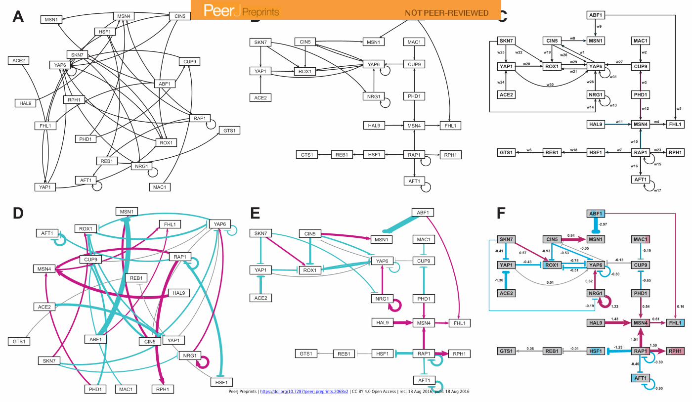
MSN1

ROX1

FHL1

GTS1 RPH1

ABF1

MAC1

CUP9

PHD1

MSN4

RAP1

AFT1

REB1 HSF1

HAL9

NRG1

YAP6

CIN5SKN7

YAP1

ACE2

w1

w31

w19

w20

w21

w8

w27w29

w30w28

w17

w16

w10

w4

w18w6

w15

w13

w23w7

w11

w3

w12

w2

w5

w9

w25

w24

w14

w22w26

MSN1

GTS1

-0.05

-0.30

-0.93

-0.43

-0.51

0.94

-0.53

-0.13-0.75

0.01 0.62

-0.90

-0.40

1.01

0.61

-0.010.08

-0.89

1.23

1.50-1.23

1.43

-0.65

0.54

-0.19

0.16

-2.97

-0.41

-1.36

-0.19

0.57

CUP9

PHD1

REB1

HAL9

NRG1

YAP6

CIN5SKN7

YAP1

ACE2

ABF1

MAC1

MSN4

RAP1

ROX1

AFT1

FHL1

HSF1 RPH1

CIN5

CUP9

FHL1GTS1

HSF1

MSN1MSN4

NRG1

RAP1

AFT1

REB1

ROX1

RPH1

YAP1

YAP6

ABF1

ACE2

HAL9

MAC1

PHD1

SKN7

CIN5

CUP9

FHL1

GTS1 HSF1

MSN1

MSN4

NRG1

RAP1

AFT1

REB1

ROX1

RPH1

YAP1YAP6

ABF1

ACE2

HAL9

MAC1

PHD1

SKN7

CIN5

CUP9

FHL1

GTS1

HSF1

MSN1

MSN4

NRG1

RAP1

AFT1

REB1

ROX1

RPH1

YAP1

YAP6

ABF1

ACE2

HAL9

MAC1PHD1

SKN7

CIN5

CUP9

FHL1

GTS1 HSF1

MSN1

MSN4

NRG1

RAP1

AFT1

REB1

ROX1

RPH1

YAP1

YAP6

ABF1

ACE2

HAL9

MAC1

PHD1

SKN7

A B C

D E F
