GEOLOGICAL SURVEY CIRCULAR 672

Ground Motion Values for Use in the Seismic Design of the Trans-Alaska Pipeline System

Ground Motion Values for Use in the Seismic Design of the Trans-Alaska Pipeline System

By Robert A. Page, David M. Boore,

William B. Joyner, and Henry W. Coulter

G E 0 L 0 G I C A L S U R V E Y C I R C U L A R 672

Washington J 972

United States Department of the Interior

THOMAS S. KLEPPE, Secretary

Geological Survey V. E. McKelvey, Director

First printing 1972

Second printing 1976

Free on application to the U.S. Geological Survey, Notional Center, Reston, Va. 22092

Figure I. 2.

3-b 3. 4. 5. b. 7.

8 • II 8. 9.

Table

10. II.

I. 2. 3. 4. 5.

CONTENTS

Page

Abstract ······---------------------------------··------···---·-··-------··-·----········----·--·-·--- I Introduction ·-------·---·-····--··--·---------------------------------------·---------------------- I Seismic potential -----------------------------------------------------------------------------· 2 Design approach ------------------------------------------------------·--·---------------------· 2 Ground motion values ---------------------------------------------------------------------· 3

Acceleration ----------------------------·------------·----------------------------------- 4 Velocity ------------------------------------------------------------------------------------· 9 Displacement ----------------------------------------·------------------------------------1 0

Duration -------------------------------------------------------------------------------------- II References ----------------------------------------·---------------------·-·------------------------13 Appendix A, Recurrence intervals -------------------------------------------------14 Appendix B, Procedure of Newmark and Hall for determination

of response spectra -------------------------------·----------·-------·---·-------------- 15 Appendix C, Ground motion data ________________________ ·--------------------------·15

ILLUSTRATIONS

Page

Map of proposed route of trans-Alaska oil pipeline showing seismic zonation and magnitudes of design eartl.~uakes ........ 2

Accelerogram from 1966 Parkfield earthquake illustrating definition of ground motion parameters .... ---·----------·---------------·--- 4 Graphs showing: Peak horizontal acceleration versus distance to slipped fault as a function of magnitude·---·-------------------------------·---·-----------·--- 5 Peak horizontal acceleration versus distance to slipped fault (or epicentral distance)_ f~r_ magnitude 5 earth~uakes .......... 6 Peak horizontal accelerations and 0.05g horizontal durations versus distance to slipped fault for 1966 Parkfiel~ earthquake 7

Peak horizontal acceleration versus distance to slipped fault (or- epicentral distance) for magnitude 6 earth~uakes .......... 8

Unfiltered and filtered accelerograms of the 1971 San Fernando earthquake --------------------------------------·------·---·--------·--------------- 9 Graphs showing: - -- ---

Peak horizontal velocity versus distance to slipped fault (or epicentral distance) for magnitudes 5, 6, and 7 .................... 10 Peak horizontal dynamic displacement versus distance to slipped fault (or epicentral distance) for mag11itudes 5, 6,

and 7 ·----------------------------------------------------------------------------- ------------·--------------------------------·------------·----------------------·---·-------·---------·--------- 12 Duration of shaking versus distance to slipped fault (or epicentral distance) for magnitudes 5, 6, and 7 ........ --------·--··--·-· 13

Examples of tripartite logarithmic ground and respome spectra ···-------------·-------·-------------------·---·-------·-·-------·--····-·-------·--········· J5

TABLES Page

Design earthquakes along the pipeline route .... -------------····---·--------··-----------------------------·-------··---------·········---···--·---·---·-······--····-···--···· 2 Near-fault horizontal ground motion .... ---···------·-------····----·-----··------··---------------------------------------·--·-···---·---····-----------·---···-··············--····· 3 Peak horizontal ground accelerations from filtered and unfiltered accelerograms at Pacoima dam ........................................ 8 Peak ground acceleration data for which distances to the causative fault are most accurately known .................................... l b Strong motion data plotted on graphs showing peak horizontal acceleration, velocity, and dynamic displaceMent and dura-

tioa of shaking as a function of distance to slipped fau It (or epicentral distance)-··--·---······---·-····--·--··-----·-·····--·---·····-····-- 19

Ill

Ground Motion Values for Use in the Seismic Design

of the T rans-Aiaska Pipeline System

By Robert A. Page, David M. Boore, William B. Joyner, and Henry W. CoultP.r

ABSTRACT The proposed trans-Alaska oil pipeline, which would

traverse the state north to south from Prudhoe Bay on the Arctic coast to Valdez on Prince William Sound, will be subject to serious earthquake hazards over much of its length. To be acceptable from an environmental standpoint, the pipeline system is to be designed to mini­mize the potential of oil leakage resulting from seismic shaking, faulting, and seismically induced ground de­formation.

The design of the pipeline system must accommodate the effects of earthquakes with magnitudes ranging from 5.5 to 8.5 as specified in the "Stipulations for Pro­posed Trans-Alaskan Pipeline System." This report characterizes ground motions for the specified earth­quakes in terms of peak levels of ground acceleration, velocity, and displacement and of duration of shaking.

Published strong motion data from the Western United States are critically reviewed to determine the intensity and duration of shaking within several kilom­eters of the slipped fault. For magnitudes 5 and 6, for which sufficient near-fault records are available, the adopted ground motion values are based on data. For larger earthquakes the values are based on extrapola­tions from the data for smaller shocks, guided by simpli­fied theoretical models of the faulting process.

INTRODUCTION The route of the proposed trans-Alaska oil

pipeline from Prudhoe Bay on the Arctic Ocean to Valdez on Prince William Sound intersects several seismically active zones. Sections of the proposed pipeline will be subject to serious earthquake hazards, including seismic shaking, faulting, and seismically induced ground defor­mation such as slope failure, differential com-

paction, and liquefaction. This rep1rt is con­cerned only with seismic shaking that, if not accommodated in the design, could c~use defor­mation leading to failure in the pipeline, storage tanks, and appurtenant structures and equiP­ment and ultimately to the leakage of oil. It might also induce effects such as seiching of liquids in storage tanks and liquefaction, land-

. sliding, and differential compaction in founda­tion materials, all of which could result in defor­mation and potential failure.

To protect the environment, the p~oeline sys­tem is to be designed so as to minirrize the po­tential of oil leakage resulting fron1 effects of earthquakes. The magnitudes of the earth­quakes which the design must accommodate are given in "Stipulations for Proposed ':':'rans-Alas­kan Pipeline System" ([U.S.] Feieral Task Force on Alaskan Oil Development, 1972, Ap-. pendix, Sec. 3.4.1, p. 55), hereinafter referred to as "Stipulations." This report ct·.~racterizes ground motions for the specified de<"1ign earth­quakes.

The seismic design of the propoe-P.d pipeline involves a combination of problems not usually encountered. In the design of important struc­tures, detailed geologic and soil inY~stigations of the site generally provide the background data. Such detailed site investigations are not economically feasible for a linear structure nearly 800 miles long. In addition, a structure more limited in extent can be located on compe­tent foundation materials and away from known

faults, whereas a pipeline traversing Alaska from north to south unavoidably crosses active faults and encounters a full range of foundation conditions from bedrock to water-saturated silty sands with a high potential for liquefaction (U.S. Geol. Survey, 1971).

SEISMIC POTENTIAL The "Stipulations" specify the earthquake

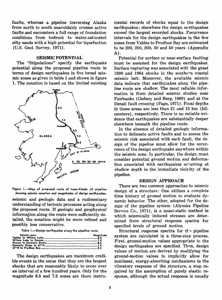
potential along the proposed pipeline route in terms of design earthquakes in five broad seis­mic zones as given in table 1 and shown in figure 1. The zonation is based on the limited existing

ALASKA

\ '

\ \ \

0 100 200 :500 400 500 KM

Figure I.-Map of proposed route of trans-Alaska oil pipeline showing seismic zonation and magnitudes of design earthquakes.

seismic and geologic data and a rudimentary understanding of tectonic processes acting along the proposed rqute. If geologic and geophysical information along the route were sufficiently de­tait'ed, the zonation might be more refined and possibly less conservative.

Table I.-Design earthqu.tkes alon;~ the pipeline route Seismic zone Magnitude

Valdez to Willow Lake____ -------------8.5 Willow Lake to Paxson_________ 7.0 Paxson to Donnelly Dom•-------------------8.0 Donnelly Dome to 67°N .7.5 67°N to Prudhoe Bay 5.5

The design earthquakes are maximum credi­ble events in the sense that they are the largest shocks that are reasonably likely to occur over an interval of a few hundred years. Only for the magnitude 8.5 and 7.5 zones are there instru-

2

mental records of shocks equal to the design earthquakes; elsewhere the design er.rthquakes exceed the largest recorded shocks. Pecurrence intervals for the design earthquakes in the five zones from Valdez to Prudhoe Bay are estimated to be 200, 200, 200, 50 and 50 years (Appendix A).

Potential for surface or near-surface faulting must be assumed for the design earthquakes. Surface rupturing was associated with the great 1899 and 1964 shocks in the southr-rn coastal seismic belt. Moreover, the available seismic data indicate that earthquakes alon~: the pipe­line route are shallow. The most reliable infor­mation is from detailed seismic studies near Fairbanks (Gedney and Berg, 1969) and at the Denali fault crossing (Page, 1971). Focal depths in these areas are less than 21 and 13 km (kil­ometers), respectively. There is no reliable evi­dence that earthquakes are substantially deeper elsewhere beneath the pipeline route"

In the absence of detailed· geologic informa­tion to delineate active faults and to assess the seismic risk associated with each fault, the de­sign of the pipeline must allow for the occur­rence of the design earthquake anywllere within the seismic zone. In particular, the design must consider potential ground motion and deforma­tion associated with earthquakes oc~urring at shallow depth in the immediate vicirity of the pipeline.

DESIGN APPROACH There are two common approaches to seismic

design of a structure: One utilizes a complete time history of ground motion to evaluate dy­namic behavior. The other, adopted for the de­sign of the pipeline system (Alyeska Pipeline Service Co., 1971), is a quasi-static method in which seismically induced stresses are deter­mined from structural response spectra for specified levels of ground motion.

Structural response spectra for tl'~ pipeline system are calculated in a three-step process. First, ground-motion values appropriate to the design earthquakes are specified. Th~n, design values of motion are derived by modifying the ground-motion values to implicitly allow for nonlinear, energy-absorbing mechanisms in the vibratory response of the structure, a step re­_quired by the assumption of purely elastic re­sponse, although the actual response is usually

inelastic and nonlinear for large ground mo­tions. Finally, smoothed tripartite logarithmic response spectra are constructed from the de­sign seismic motions by the general procedure of Newmark and Hall (1969), outlined in Ap­pendix B.

The initial step in the design process discussed herein characterizes ground motion appropriate to the design earthquakes. This step is based solely on seismological data and principles and does not incorporate factors dependent on soil­structure interactions, deformational processes within structures, or the importance of the structures to be designed. It involves scientific data and interpretation, whereas the subsequent steps involve engineering, economic, and social judgments relating to the nature and value of the structures.

The choice of parameters with which to spec­ify ground motion was guided by the design ap­proach adopted for the pipeline project. A use­ful set for the derivation of tripartite structural response spectra includes acceleration, velocity, displacement, and duration of shaking.

GROUND MOTION VALUES

Table 2 characterizes near-fault horizontal ground motion for the design earthquakes. The intensity of shaking is described by maximum values of ground acceleration, velocity, and dis­placement. In addition to the maximum acceler­ation, levels of absolute acceleration exceeded or attained two, five, and ten times are specified, because a single peak of intense motion may contribute less to the cumulative damage po­tential than several cycles of less intense shak­ing. Levels of absolute velocity

41exceeded or

attained two and three times are also given.

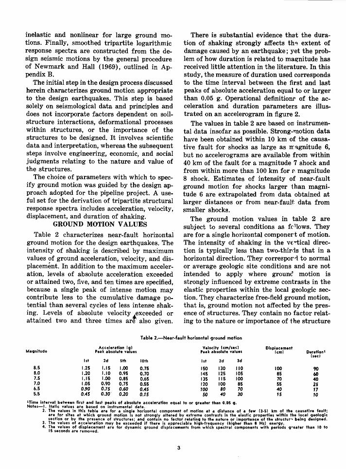
There is substantial evidence that the dura­tion of shaking strongly affects tha. extent of damage caused by an earthquake; yet the prob­lem of how duration is related to magnitude has received little attention in the literature. In this study, the measure of duration used corresponds to the time interval between the first and last peaks of absolute acceleration equal to or larger than 0.05 g. Operational definitionr of the ac­celeration and duration parameters are illus­trated on an accelerogram in figure 2.

The values in table 2 are based on instrumen­tal data insofar as possible. Strong-motion data have been obtained within 10 km of the causa­tive fault for shocks as large as rr.~gnitude 6, but no accelerograms are available from within 40 km of the fault for a magnitude 7 shock and from within more than 100 km for r. magnitude 8 shock. Estimates of intensity of near-fault ground motion for shocks larger than magni­tude 6 are extrapolated from data obtained at larger distances or from near-fault data from smaller shocks.

The ground motion values in table 2 are subject to several conditions as fC'llows. They are for a single horizontal componert of motion. The intensity of shaking in the vr-rtical direc­tion is typically less than two-thirds that in a horizontal direction. They correspor1 to normal or average geologic site conditions and are not intended to apply where grounc motion is strongly influenced by extreme contrasts in the elastic properties within the local geologic sec­tion. They characterize free-field ground motion, that is, ground motion not affected by the pres­ence of structures. They contain no factor relat­ing to the nature or importance of the structure

Table 2.-Near-fault horizontal ground motion

Acceleration (g) Velocity (em/sec) Displacement Magnitude Peak absolute values Peak absolute values (em) Durationl

(sec I 1st 2d 5th lOth 1st 2d 3d

8.5 1.25 1.15 1.00 0.75 150 130 110 100 90 8.0 1.20 1.10 0.95 0.70 145 125 105 85 60 7.5 1.15 1.00 0.85 0.65 135 115 100 70 40 7.0 1.05 0.90 0.75 0.55 120 100 85 55 25 6.5 0.90 0.75 0.60 0.45 100 80 70 40 17 5.5 0.45 0.30' 0.20 0.15 50 40 30 15 10

1Time interval between first and last peaks of absolute acceleration equal to or greater than 0.05 g. Notes-1. Italic values are based on instrumental data.

2. The values in this table are for a single horizontal component of motion at a distance of a few 13-51 km of the causative fault; are for sites at which ground motion is not strongly altered by extreme contrasts in the elastic properties within the local geologic section or by the presence of structures; and contain no factor relating to the nature or importance of the structur" being designed.

3. The values of acceleration may be exceeded if there is appreciable high-frequency (higher than 8 Hz) energy. 4. The values of displacement are for dynamic ground displace"'ents from which spectral components with periods gpeater than 10 to

15 seconds are removed.

3

5

-4 ltlo

(j) TIME ( SECONDS)

3 4 ® To.oeg

Figure 2.-Accelerogram from 1966 Parkfield earthquake illustrating definition of parameters referred to in table 2. Peaks O"" accelero­gram are numbered consecutively I through 10 in order of decreasing amplitude. First, second, fifth, and tenth highest peaks are listed in table 2. Duration, To.osg• is the time interval between the first and last peaks of acceleration equal to or greater than 0.05 gin absolute value.

being designed. They are not the maximum pos­sible. As mentioned in the following section, very little reliable data have been obtained with­in 10 km of the causative fault. How often these values are likely to be exceeded cannot be re­liably estimated from the currently existing data. The acceleration values may be exceeded if there is appreciable energy in frequencies higher than 8 Hz (cycles per second) . The dis­placement values correspond to dynamic ground displacements, as would be recorded on a strong­motion instrument having a frequency response flat to ground displacement for periods less than 10 to 15 seconds.

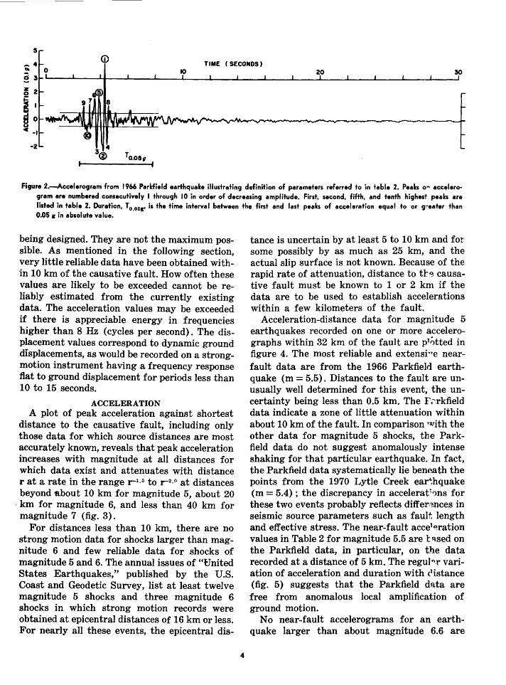
ACCELERATION A plot of peak acceleration against shortest

distance to the causative fault, including only those data for which source distances are most accurately known, reveals that peak acceleration increases with magnitude at all distances for which data exist and attenuates with distance r at a rate in the range r-1 •

5 to r-2 · 0 at distances beyond 1tbout 10 km for magnitude 5, about 20

· km for magnitude 6, and less than 40 km for magnitude 7 (fig. 3).

For distances less than 10 km, there are no strong motion data for shocks larger than mag­nitude 6 and few reliable data for shocks of magnitude 5 and 6. The annual issues of "Bnited States Earthquakes," published by the U.S. Coast and Geodetic Survey, list at least twelve magnitude 5 shocks and three magnitude 6 shocks in which strong motion records were obtained at epicentral distances of 16 km or less. For nearly all these events, the epicentral dis-

4

tance is uncertain by at least 5 to 10 km and for some possibly by as much as 25 km, and the actual slip surface is not known. Because of the rapid rate of attenuation, distance to t:r~ causa­tive fault must be known to 1 or 2 km if the data are to be used to establish accelerations within a few kilometers of the fault.

Acceleration-distance data for magnitude 5 earthquakes recorded on one or more accelero­graphs within 32 km of the fault are p1otted in figure 4. The most reliable and extensi .. Te near-fault data are from the 1966 Parkfield earth­quake (m = 5.5). Distances to the fault are un­usually well determined for this event, the un­certainty being less than 0.5 km. The F~--.rkfield data indicate a zone of little attenuation within about 10 km of the fault. In comparison with the other data for magnitude 5 shocks, the Park­field data do not suggest anomalously intense shaking for that particular earthquake. In fact, the Parkfield data systematically lie beneath the points from the 1970 Lytle Creek ear.hquake (m = 5.4) ; the discrepancy in accelerat~~ns for these two events probably reflects di:ffer~~nces in seismic source parameters such as fault length and effective stress. The near-fault acce1~ration

values in Table 2 for magnitude 5.5 are l: f.l.sed on the Parkfield data, in particular, on the data recorded at a distance of 5 km. The regu]".r vari­ation of acceleration and duration with clistance (fig. 5) suggests that the Parkfield data are free from anomalous local amplification of ground motion.

No near-fault accelerograms for an earth­quake larger than about magnitude 6.6 are

0

1.0

0.52g

0.08 km

- 0.1 t:), -z 0 .... <( 0:: w ....J w u u <(

0.01 EARTHQUAKE

MAGNITUDE

• 5.0-5.9 0 6.0-6.9 • 7.0-7.9

10

0 0 2

DISTANCE (KM)

0

o• CJ)i 0

mo• •

o•~ 0 o. 0

~

i •

0

• ••

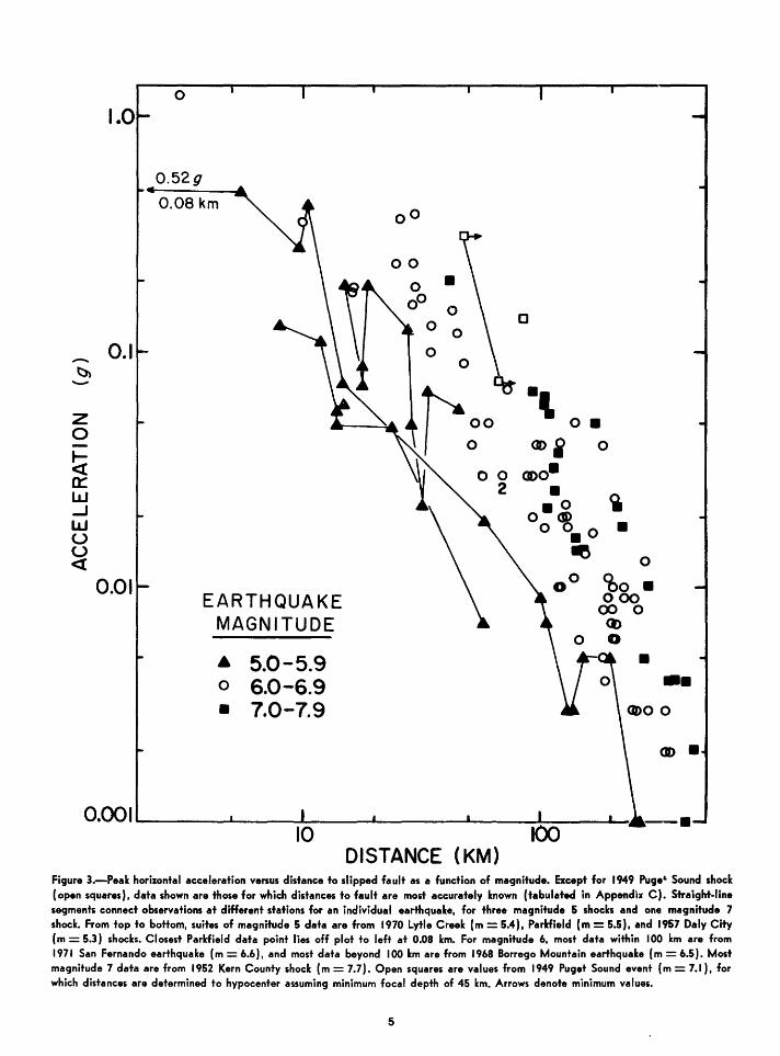
Figure 3.-Peak horizontal acceleration versus distance to slipped fault as a function of magnitude. Except for 1949 Puge' Sound shock (open squares), data shown are those for which distances to fault are most accurately known (tabulated in Appendix C). Straight-line segments connect observations at different stations for an individual earthquake, for three magnitude 5 shocks and one magnitude 7 shock. From top to bottom, suites of magnitude 5 data are from 1970 Lytle Creek (m = 5.4), Parkfield (m = 5.5), and 1957 Daly City (m = 5.3) shocks. Closest Parkfield data point lies off plot to left at 0.08 km. For magnitude 6, most data within 100 km are from 1971 San Fernando earthquake (m = 6.6), and most data beyond 100 km are from 1968 Borrego Mountain earthquake (m = 6.5). Most magnitude 7 data are from 1952 Kern County shock (m = 7.7). Open squares are values from 1949 Puget Sound event (m = 7.1 ), for which distances are determined to hypocenter assuming minimum focal depth of 45 km. Arrows denote minimum values.

5

~

z 0 MAGNITUDE 5.0-5.9 0

.... <t EXPLANATION 0::

0

UJ • ...J UJ o• u Distance to fault known 0 u within 2 km 0 <t .,

0 0

Distance to fault known 0 J! 2 2o 0

within 5 km ...... 0 0

t Distance to fault known 0

within 25 km

0.1 1.0 10 100 DISTANCE (KM)

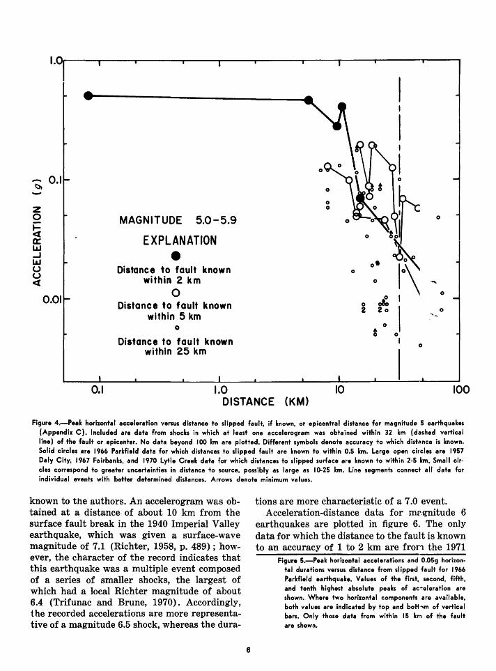
Figure 4.-Peak horizontal acceleration versus distance to slipped fault, if known, or epicentral distance for magnitude 5 earthquakes (Appendix C). Included are data from shocks in which at least one accelerogram was obtained within 32 km (dashed vertical line) of the fault or epicenter. No data beyond 100 km are plotted. Different symbols denote accuracy to which dist11nce is known. Solid circles are 1966 Parkfield data for which distances to slipped fault are known to within 0.5 km. Large open circles are 1957 Daly City, 1967 Fairbanks, and 1970 Lytle Creek data for which distances to slipped surface are known to within 2-5 km. Small cir­cles correspond to greater uncertainties in distance to source, possibly as large as I 0-25 km. Line segments connect all data for individual events with better determined distances. Arrows denote minimum values.

known to the authors. An accelerogram was ob­tained at a distance· of about 10 km from the surface fault break in the 1940 Imperial Valley earthquake, which was given a surface-wave magnitude of 7.1 (Richter, 1958, p. 489) ; how­ever, the character of the record indicates that this earthquake was a multiple event composed of a series of smaller shocks, the largest of which had a local Richter magnitude of about 6.4 (Trifunac and Brune, 1970). Accordingly, t be recorded accelerations are more representa­tive of a magnitude 6.5 shock, whereas the dura-

6

tions are more characteristic of a 7.0 event. Acceleration-distance data for mr.gnitude 6

earthquakes are plotted in figure 6. The only data for which the distance to the fault is known to an accuracy of 1 to 2 km are fron the 1971

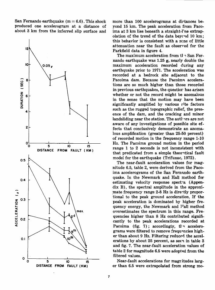
Figure 5.-Peak horizontal accelerations and O.OSg horizon­tal durations versus distance from slipped fault for 1966 Parkfield earthquake. Values of the first, second, fifth, and tenth highest absolute peaks of ac-:-eleration are shown. Where two horizontal components are available, both values are indicated by top and botbm of vertical bars. Only those data from within 15 k111 of the fault are shown.

San Fernando earthquake (m = 6.6). This shock produced one accelerogram at a distance of about 3 km from the inferred slip surface and

~

z 2 1-<( a: 1.&.1 _. 1.&.1 0 0 <(

0 1.&.1 (/)

z 0 6 fi a: ::) 0

4

2

o~------~------L-------~---0 5 ~ 15

DISTANCE FROM FAULT ( KM)

0.5

0.4

0.3

0.2

0.1

5 ~ ~ DISTANCE FROM FAULT (KM)

7

more than 100 accelerograms at dirtances be­yond 15 km. The peak acceleration from Paco­ima at 3 km lies beneath a straight-Pne extrap­olation of the trend of the data bey<'"ld 10 km; this behavior is consistent with a zone of little attenuation near the fault as obserYed for the Parkfield data in figure 4.

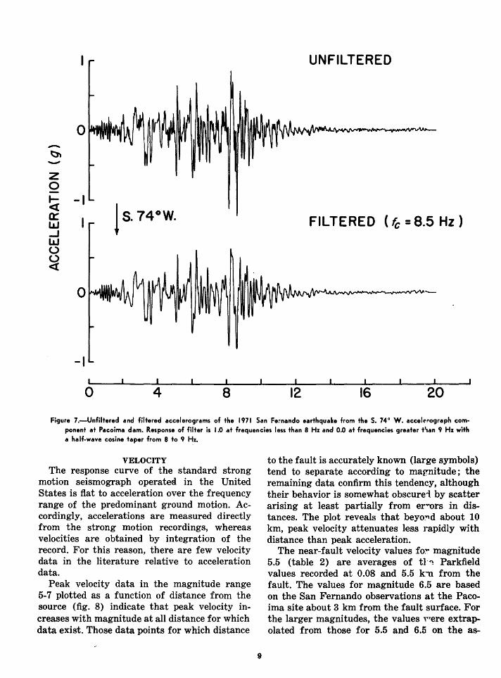
The maximum acceleration from t]'~ San Fer­nando earthquake was 1.25 g, nearly double the maximum acceleration recorded during any earthquake prior to 1971. The accel~ration was recorded at a bedrock site adjac~nt to the Pacoima dam. Because the Pacoim~ accelera­tions are so much higher than those recorded in previous earthquakes, the questior has arisen whether or not the record might be anomalous in the sense that the motion may have been significantly amplified by various rite factors such as the rugged topographic relief, the pres­ence of the dam, and the cracking and minor landsliding near the station. The autl''lrs are not aware of any investigations of possible site ef­fects that conclusively demonstrate an anoma­lous amplification (greater than 25-50 percent) of recorded motion in the frequency range 1-10 Hz. The Pacoima ground motion in the period range 1 to 2 seconds is not inconsistent with that predicated from a simple theor~tical fault model for the earthquake (Trifunac, 1972).

The near-fault acceleration values for mag­nitude 6.5, table 2, were derived frmn the Paco­ima accelerograms of the San Fern.~ndo earth­quake. In the Newmark and Hall method for estimating velocity response spect:-:-a (Appen­dix B), the spectral amplitude in the approxi­:mate frequency range 2-8Hz is dire~tly propor­tional to the peak ground acceleration. If the peak acceleration is dominated by higher fre­quency energy, the Newmark and Pall method overestimates the spectrum in this range. Fre­quencies higher than 8 Hz contributed signifi­cantly to the peak accelerations recorded at Pacoima (fig. 7) ; accordingly, tl'~ accelero­grams were filtered to remove frequ~ncies high­er than about 9Hz. Filtering reducf'q the accel­erations by about 25 percent, as se£n in table 3 and fig. 7. The near-fault acceleration values of table 2 for magnitude 6.5 were adopt~d from the filtered values.

Near-fault accelerations for magr.itudes larg­er than 6.5 were extrapolated from strong mo-

z 0

~ a:: L&J 0.1 ..J L&J 0 0 <(

• 0

0

0

MAGNITUDE 6.0-6.9 EXPLANATION • Distance to fault known

within 2 km 0

Distance to fault known within 5 km

0

Distance to fault known

I ., ~ ••

•• I • -• • ••• 2 •

• 0 01 within 25 km . ~----------~--~----~----~-----L~~ 1.0 10

DISTANCE (KM)

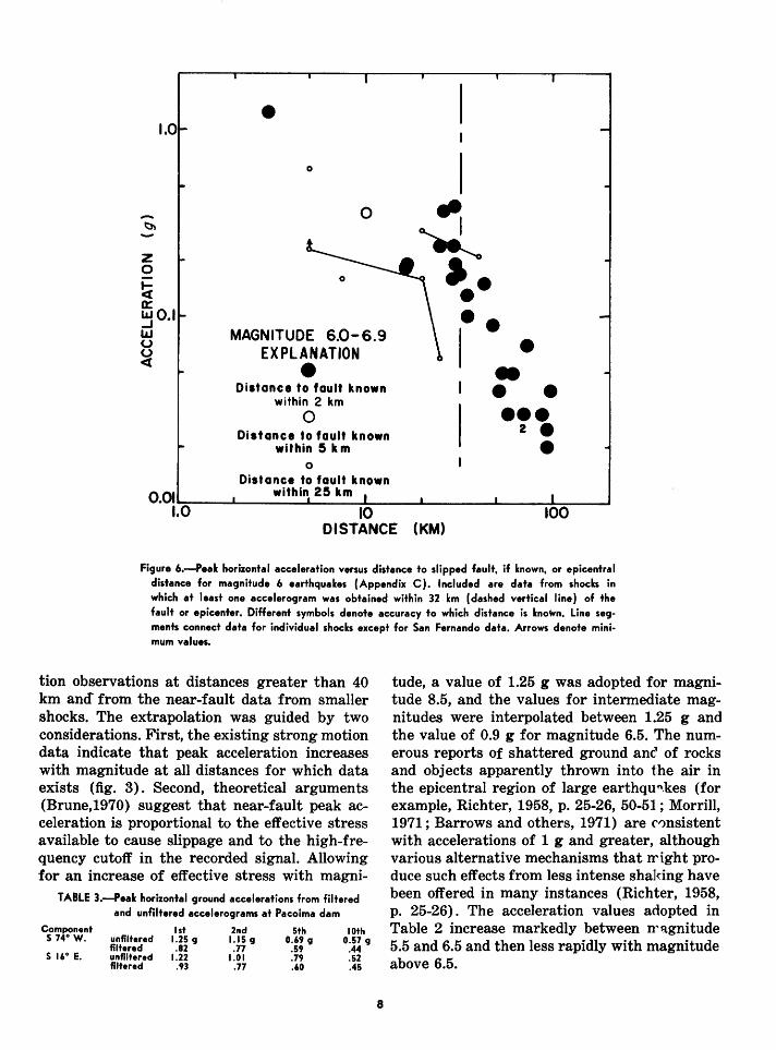
Figure 6.-Peak horizontal acceleration versus distance to slipped fault, if known, or epicentral distance for magnitude 6 earthquakes (Appendix C). Included are data from shocks in which at least one accelerogram was obtained within 32 km (dashed vertical line) of the fault or epicenter. Different symbols denote accuracy to which distance is known. Line seg­ments connect data for individual shocks except for San Fernando data. Arrows denote mini­mum values.

tion observations at distances greater than 40 km and from the near-fault data from smaller shocks. The extrapolation was guided by two considerations. First, the existing strong motion data indicate that peak acceleration increases with magnitude at all distances for which data exists (fig. 3). Second, theoretical arguments (Brune,1970) suggest that near-fault peak ac­celeration is proportional to the effective stress available to cause slippage and to the high-fre­quency cutoff in the recorded signal. Allowing for an increase of effective stress with magni-

TABLE 3.-Peak horizontal ground accelerations from filtered

Component s 74° w.

and unfiltered accelerograms at Pacoima dam

1st 2nd 5th unfiltered 1.25 CJ 1.15 CJ 0.69 g filtered .82 . 77 .59 unfiltered 1.22 1.0 I . 79 filtered .93 .77 .60

lOth 0.57 g

.44

.52 .45

8

tude, a value of 1.25 g was adopted for magni­tude 8.5, and the values for intermediate mag­nitudes were interpolated between 1.25 g and the value of 0.9 g for magnitude 6.5. The num­erous reports of shattered ground anc, of rocks and objects apparently thrown into the air in the epicentral region of large earthquq.kes (for example, Richter, 1958, p. 25-26, 50-51 ; Morrill, 1971; Barrows and others, 1971) are c0nsistent with accelerations of 1 g and greater, although various alternative mechanisms that rright pro­duce such effects from less intense shaking have been offered in many instances (Richter, 1958, p. 25-26) . The acceleration values adopted in Table 2 increase markedly between n'agnitude 5.5 and 6.5 and then less rapidly with magnitude above 6.5.

--z 0

0

~ -1

ffi I ..J LLI (.) (.) <(

0

-I

0

UNFILTERED

FILTERED ( fc = 8.5 Hz )

4 8 12 16 20

Figure 7.-Unfiltered and filtered accelerograms of the 1971 San Fe~nando earthquake from the S. 74° W. accelrrograph com­ponent at Pacoima dam. Response of filter is 1.0 at frequencies less than 8 Hz and 0.0 at frequencies greater t'-lan 9 Hz with a half-wave cosine taper from 8 to 9 Hz.

VELOCITY The response curve of the standard strong

motion seismograph operates in the United States is flat to acceleration over the frequency range of the predominant ground motion. Ac­cordingly, accelerations are measured directly from the strong motion recordings, whereas velocities are obtained by integration of the record. For this reason, there are few velocity data in the literature relative to acceleration data.

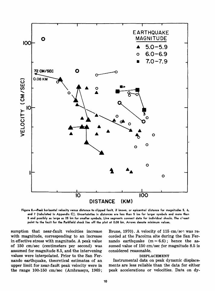
Peak velocity data in the magnitude range 5-7 plotted as a function of distance from the source (fig. 8) indicate that peak velocity in­creases with magnitude at all distance for which data exist. Those data points for which distance

9

to the fault is accurately known (large symbols) tend to separate according to magnitude; the remaining data confirm this tendency, although their behavior is somewhat obscurei by scatter arising at least partially from er:-·ors in dis­tances. The plot reveals that beyo~d about 10 km, peak velocity attenuates less rapidly with distance than peak acceleration.

The near-fault velocity values fo:':" magnitude 5.5 (table 2) are averages of t1''1 Parkfield values recorded at 0.08 and 5.5 kn from the fault. The values for magnitude 6.5 are based on the San Fernando observations at the Paco­ima site about 3 km from the fault surface. For the larger magnitudes, the values y•ere extrap­olated from those for 5.5 and 6.5 on the as-

-0 w en ' :E 0 -0 0 ..J w >

0

72~/SEC 0

~ 0

EARTHQUAKE MAGNITUDE A 5.0-5.9 0 6.0-6.9

• 7.0-7.9

0

0 0

0

0

DISTANCE (KM)

Figure 8.-Peak horizontal velocity versus distance to slipped fault, if known, or epicentral distance for magnitudes 5, 6, and 7 {tabulated in Appendix C). Uncertainties in distances are less than 5 km for larger symbols and more than 5 and possibly as large as 25 km for smaller symbols. Line segments connect data for individual shocks. The c1,sest point to the fault for the Parkfield shock lies off the plot at 0.08 km. Arrows denote minimum values.

sumption that near-fault velocities increase with magnitude, corresponding to an increase in effective stress with magnitude. A peak value of 150 em/sec (centimeters per second) was assumed for magnitude 8.5, and the intervening values were interpolated. Prior to the San Fer­nando earthquake, theoretical estimates of an upper limit for near-fault peak velocity were in the range 100-150 em/sec (Ambraseys, 1969;

10

Brune, 1970). A velocity of 115 cm/sE'~ was re­corded at the Pacoima site during the San Fer­nando earthquake (m = 6.6); hence the as­sumed value of 150 em/sec for magnitude 8.5 is considered reasonable.

DISPLACEMENT Instrumental data on peak dynamic: displace­

ments are less reliable than the data for either peak accelerations or velocities. Data on dy-

namic displacements excluding spectral compo­nents with periods greater than about 10-15 seconds are available from double integration of accelerograms or directly fr-om displacement meters. Both types of data are subject to uncer­tainties. In the double integration of digitized accelerograms, errors may arise from low-fre­quency noise in the digitization of the original accelerogram and from lack of knowledge of the true baseline of the accelerogram. On the other hand, there are instrumental difficulties associ­ated with displacement meters operating with a free period of 10 seconds. The rel~tive accuracy of the two types of data is not adequately un­derstood (Hudson, 1970).

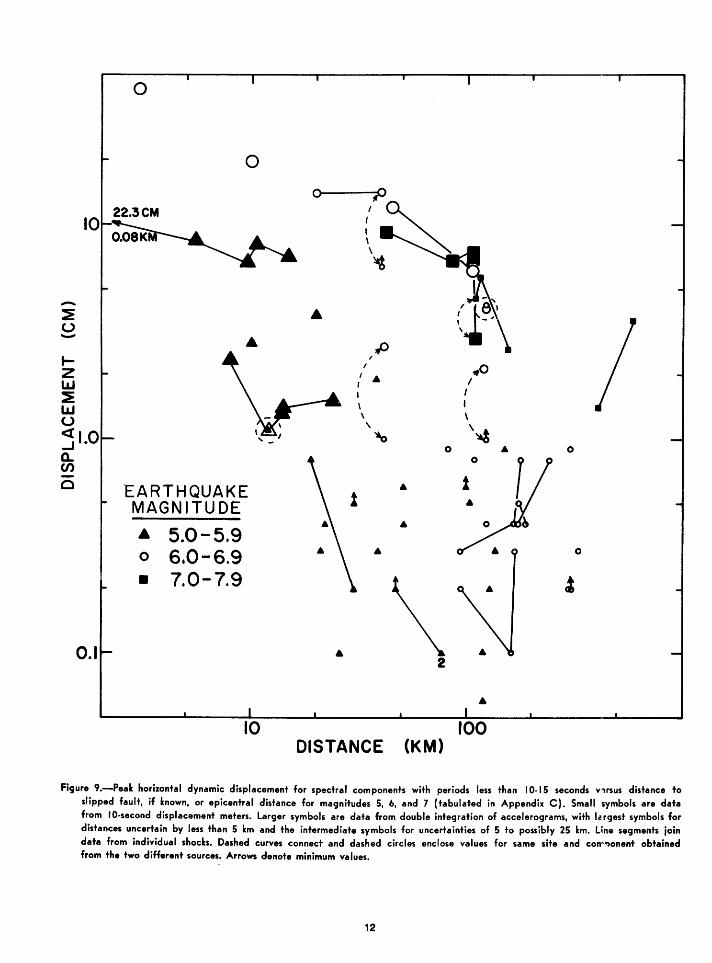
Peak displacement data obtained from double integration of accelerograms and from 10-sec­ond displacement meters when plotted against distance (fig. 9) show no apparent systematic difference between the two types of data within the scatter of the points. Peak displacement at a given distance from the fault, like peak accel­eration and velocity, increases with magnitude.

The near-fault value of peak displacement for magnitude 5.5 (table 2) is the mean of the Park­field values obtained at 0.08 and 5.5 km from the fault. For magnitude 6.5 the value is based on the Pacoima record for the San Fernando earthquake. How peak dynamic displacement (for periods less than 10-15 seconds) scales with magnitude for larger shocks is uncertain. An upper limit to the increase of near-fault dynam­ic displacement with magnitude is the rate at which fault dislocation increases with magni­tude. The total fault slip in the 1964 Alaska shock (m=8.5) is estimated to have been about five times that in the 1971 San Fernando earth­quake (m=6.5). Hence, an upper bound" on the peak dynamic displacement for magnitude 8.5, after removal of low frequency energy, is about 2m. In this study, a value of 1m is assumed for magnitude 8.5, and the values between mag­nitude 6.5 and 8.5 are smoothly interpolated.

DURATION The measure of duration used in this study

is the time interval between the first and last acceleration peaks equal to or greater than 0.05 g. Although crude, this measure is readily ap­plied to the existing accelerograms and approxi­mates the cumulative time over which the ground accelerations exceed a given level. Com­parison of felt reports for earthquakes of mag-

11

nitude 5 and 6 with near-fault accele:-:-ograms from shocks of similar magnitude suggest that the "intense" or "strong" phase of shaking men­tioned in felt reports corresponds to accelera­tions of about 0.05 g and greater. In comoarison, the minimum perceptible level of accele:-:-ation is 0.001 g (Richter, 1958, p. 26).

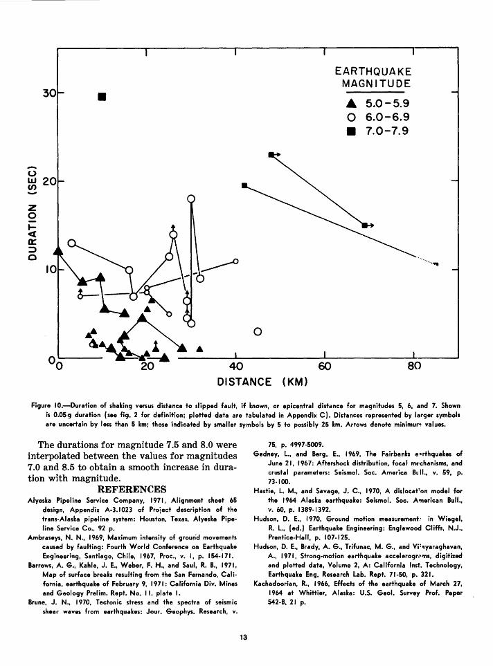
Durations obtained for several earthquakes in the magnitude range 5-7 indicate tll at for a given magnitude, duration decreases with in­creasing distance from the source, and that at a given distance from the source, duration in­creases for larger magnitudes (fig. 10). The 0.05 g duration for magnitude 5.5 (table ~:) is the mean of the maximum durations for the 1966 Parkfield shock (m = 5.5) recorded at distances of 0.08 and 5.5 km from the fault surface (fig. 5). The durations for magnitude 6.5 and 7.0 are based respectively on the measured O.Of g dura­tions of 13 seconds at Pacoima dam in the 1971 San Fernando earthquake (m = 6.6) and of 30 seconds at El Centro in the 1940 Imperial Valley earthquake, which was a multiple event charac­terized by a surface-wave magnitude of 7.1. These data were smoothed slightly to obtain a regular increase of duration with magnitude in table 2. The adopted near-fault durations of 17 and 25 seconds for magnitudes 6.5 and 7.0 are consistent with the duration data in figure 10 within the scatter of the points.

In the absence of near-fault data for larger magnitudes, durations can be estimated from theoretical calculations in corroboration with feit observations. Assume that a magnitude 8.5 earthquake is a multiple event comr~ised of several shocks as large as magnitude 7.5 distri­buted along a fault 500-1,000 km in len~~th. Peak accelerations of 0.05 g or greater are expected for a magnitude 7.5 earthquake at distances up to 100 km (fig. 3). For a rupture propagation velocity of 2 to 3.5 km/sec, the 0.05 g duration at a near-fault station near the center of the fault would be 100 to 57 seconds, respectively. In comparison, felt reports of the duration of intense· shaking in the aftershock zor~ of the 1964 Alaska earthquake (m = 8.5) ranged from 60-90 seconds at Whittier (Kachadoorir.n, 1966) to 150 seconds at Kodiak (Kachadoo~ian and Plafker, 1967). The tabulated duration of 90 seconds for magnitude 8.5 (table 2) is c~1nsistent with the calculated range of values and with felt data from the 1964 shock.

0

-::E u - p ~ " I .o z I

w I ~ I

:E I I

w \ I \ \ u \

\~ :51.0 ' ~ 0 A 0

~ en 0 EARTHQUAKE

MAGNITUDE A 5.0-5.9

A

0 6.0-6.9 • 0

• 7.0-7.9

\ ci

0.1 • 2

•

DISTANCE (KM)

Figure 9.-Peak horizontal dynamic displacement for spectral components with periods less than I 0-15 seconds v,,rsus distance to slipped fault, if known, or epicentral distance for magnitudes 5, b, and 7 (tabulated in Appendix C). Small symbols are data from 10-second displacement meters. Larger symbols are data from double integration of accelerograms, with largest symbols for distances uncertain by less than 5 km and the intermediate symbols for uncertainties of 5 to possibly 25 km. line segments join data from individual shocks. Dashed curves connect and dashed circles enclose values for same site and corr"onent obtained from the two different sources. Arrows denote minimum values.

12

30

-0 UJ 20 (/) -z 0 ..... <( 0:: :::) 0

•

0

EARTHQUAKE MAGNITUDE

• 5.0-5.9 0 6.0-6.9 • 7.0-7.9

40 60 80 DISTANCE (KM)

Figure 10.-Duration of shaking versus distance to slipped fault, if known, or epicentral distance for magnitudes 5, 6, and 7. Shown is O.OSg duration (see fig. 2 for definition; plotted data are tabulated in Appendix C). Distances represented by larger symbols are uncertain by less than 5 km; those indicated by smaller symbols by 5 to possibly 25 km. Arrows denote minimun values.

The durations for magnitude 7.5 and 8.0 were interpolated between the values for magnitudes 7.0 and 8.5 to obtain a smooth increase in dura­tion with magnitude.

REFERENCES Alyeska Pipeline Service Company, 1971, AI ignment sheet 65

design, Appendix A-3.1023 of Proiect description of the trans-Alaska pipeline system: Houston, Texas, Alyeska Pipe­line Service Co., 92 p.

Ambraseys, N. N., 1969, Maximum intensity of ground movements caused by faulting: Fourth World Conference on Earthquake Engineering, Santiago, Chile, 1967, Proc., v. I, p. 154-171.

Barrows, A. G., Kahle, J. E., Weber, F. H., and Saul, R. B., 1971, Map of surface breaks resulting from the San Fernando, Cali­fornia, earthquake of February 9, 1971: California Div. Mines and Geology Prelim. Rept. No. II, plate I.

Brune, J. N., 1970, Tectonic stress and the spectra of seismic shear waves from earthquakes: Jour. Geophys. Research, v.

13

75, p. 4997-5009. Gedney, L., and Berg, E., 1969, The Fairbanks e .. rthquakes of

June 21, 1967: Aftershock distribution, focal mE'chanisms, and crustal parameters: Seismol. Soc. America Bull., v. 59, p. 73-100.

Hastie, L. M., and Savage, J. C., 1970, A dislocat~on model for the 1964 Alaska earthquake: Seismol. Soc. Aonerican Bull., v. 60, p. 1389-1392.

Hudson, D. E., 1970, Ground motion measurement~ in Wiegel, R. L., (ed.) Earthquake Engineering: Englewood Cliffs, N.J., Prentice-Hall, p. I 07-125.

Hudson, D. E., Brady, A. G., Trifunac, M. G., and VP<tyaraghavan, A., 1971, Strong-motion earthquake accelerogr<"'rtS, digitized and plotted data, Volume 2, A: California lnst. Technology, Earthquake Eng. Research Lab. Rept. 71-50, p. 321.

Kachadoorian, R., 1966, Effects of the earthquake of March 27, 1964 at Whittier, Alaska: U.S. Geol. Survey Prof. Paper 542-B, 21 p.

Kachadoorian, R., and Plafker, G., 1967, Effects of the earth­quake of March 27, 1964 on the communities of Kodiak and nearby islands: U.S. Geol. Survey Prof. Paper 542-F, 41 p.

Morrill, B. J., 1971, Evidence of record vertical accelerations at Kagel Canyon during the earthquake, in The San Fernando, California, earthquake of February 9, 1971: U.S. Geol. Survey Prof. Paper 733, p. 177-181.

Newmark, N. M., and Hall, W. J., 1969, Seismic design criteria for nuclear reactor facilities: Fifth World Conference on Earthquake Engineering, Santiago, Chile, 1967, Proc., v. 2, p. 37-50.

Page, R. A., 1971, Microearthquakes on the Denali fault near the Richardson Highway, Alaska [abs.]: Am. Geophys. Union Trans., v. 52, p. 278.

-- 1972, Crustal deformation on the Denali fault, Alaska, 1942-1970: Jour. Geophys. Research, v. 77, p. 1528-1533.

Plafker, G., 1969, Tectonics of the March 27, 1964 Alaska earth­quake: U.S. Geol. Survey Prof. Paper 543-1, p. 174.

Richter, C. F., 1958, Elementary Seismology; San Francisco, W. H. Freeman and Co., 768 p.

Richter, D. H. and Matson, N. A., 1971, Quaternary faulting in the eastern Alaska Range: Geol. Soc. America Bull., v. 82, p. 1529-1539.

Stout, J. H., Brady, J. B., Weber, F., and Page, R. A., 1972, Evi­dence for Quaternary movement on the McKinley strand of the Denali fault in the Delta River area, Alaska: Geol. Soc. America Bull. (in press).

Sykes, L. R., 1972, Aftershock zones of great earthquakes, seismi­city gaps, and earthquake prediction for Alaska and the Aleutians: Jour. Geophys. Research, v. 76, p. 8021-8041.

Trifunac, M. D., 1972, Stress estimates for the San Fernando, California, earthquake of February 9, 1971: Main event and thirteen aftershocks: Seismol. Soc. America Bull., v. 62, p. 721-750.

Trifunac, M. D., and Brune, J. N., 1970, Complexity of energy release during the Imperial Valley, California earthquake of 1940: Seismol. Soc. America Bull., v. 60, p. 137-160.

[U.S.] Federal Task Force on Alaskan Oil Development, 1972, Introduction and summary, v. I ol Final environmental impact statement, proposed trans-Alaska pipeline: U.S. Dept. Interior interagency rept., 386 p.; available only from the Natl. Tech. lnf. Service, U.S. Dept. Commerce, Springfield, Va., NTIS PB-206921-1.

U.S. Geological Survey, 1971, Preliminary engineering geologic maps of the proposed trans-Alaska pipeline route [compiled by 0. J. Ferrians, R. Kachadoorian, and F. R. Weber]: U.S. Geol. Survey open-file report.

Wiggins, J. H., 1964, Effect of site conditions on earthquake intensity: American Soc. Civ. Eng., Structural Div., v. 90, p. 279-313.

APPENDIX A-RECURRENCE INTERVALS Estimates of recurrence intervals for the de­

sign earthquakes are based on the historic seis­mic record and tectonic arguments. In the inter­pretation of the seismic history, the width of each seismic zone transverse to the pipeline route is assumed to be equal to the characteris­tic length of faulting for the specified magni-

14

tude. In the southern coastal zone, earthquakes as

large as the design earthquakes occurred in 1899 near Yakutat Bay and in 1964 in Prince William Sound. This pattern is consistent with a recurrence interval of less than 100 years; however, tectonic considerations irrlicate that the average long-term interval beh<~Teen design earthquakes is longer. In the framework of glo­bal tectonics, the 12 m of thrusting involved in the 1964 earthquake (Hastie and Savage, 1970) would require 200 years of stPain accumulation at the local convergence rate of 6 cn/yr (centi­meters per year) for the Pacific and North American plates. Geologic evidence. of vertical movements in Prince William Sound (Plafker, 1969) indicates episodes of tectonic deforma­tion between quiescent periods of t.he order of 800 years. On Middleton Island the total uplift in each deformational episode is 2.5-3 times that for the 1964 earthquake. The geolo~ic evidence suggests a long-term average recmTence inter­val of about 300 years for an event comparable to the 1964 earthquake. An interval of 200 years is adopted for the magnitude 8.5 zone. The lack of seismic activity in the area between Yakutat Bay and the 1964 aftershock zone. during the past 50 years has led Sykes (1972) to identify this part of the Aleutian-Alaskan seismic belt as a likely site of a future earthquake larger than magnitude 7.

The magnitude 8.0 zone includes the Denali fault system, an active strike-slip system that displays geologic evidence for an average Holo­cene slip rate of at least 3 cm/yr (Richter and Matson, 1971). Assumption of a 6~m offset for a magnitude 8.0 event and a 3 cm/yr slip rate gives a recurrence interval of 200 years. The lack of observable fault-slip and teleseismically recorded earthquakes on the fault system in the vicinity of the pipeline route and to the east indicates that the fault system ]'as been ef­fectively locked for at least 30 ~rears (Page, 1972). An undeformed neoglacial n1oraine lying athwart the recently active fault trace is evi­dence that no major episode of faulting has occurred within the past 170 year~ (Stout and others, 1972).

Understanding of the tectonic f':'amework of the magnitude 7.5 zone is not adequate for esti­mating recurrence intervals. Ona. shock ap-

proaching the design magnitude has occurred on the pipeline route in this century, a magni­tude 7.3 shock in 1937. A recurrence interval of 50 years is assumed.

In the magnitude 7.0 and 5.5 zones, there is no historic record of shocks as large as the de­sign earthquakes. For the Willow Lake to Pax­son zone, the record of earthquakes equal to or larger than magnitude 7.0 is probably complete for at least 50 years. From 67° N to Prudhoe Bay, the record for events as small as magni­tude 5.5 is possibly complete since 1935, when a seismic station was established at College. Recurrence intervals of 200 and 50 years are assumed for the two zones.

APPENDIX B-PROCEDURE OF NEWMARK AND HALL FOR DETERMINATION OF

RESPONSE SPECTRA A response spectrum for a given level of

damping is defined by the maximum responses (usually expressed in terms of displacement, velocity, or acceleration) of linear, single-de­gree-of-freedom oscillators (with different free periods but identical values of damping) when subjected to a specified time history of ground motion. A single spectrum is a plot of the maxi­mum responses as a function of oscillator period or frequency; there is a different response spec­trum for each level of damping. The_ usefulness of the response spectrum comes from the ability to model engineering structures by equivalent simple damped oscillators and to estimate stresses induced by the particular ground mo­tion from knowledge of the equivalent period and damping of the structure and of the appro­priate response spectrum.

The values of parameters describing the ac­tual ground motion may be modified for non­linear energy-absorbing mechanisms before be­ing used in the construction of a response spec­trum. In the following example of the Newmark and Hall method for constructing response spec­tra, the ground motion values are not modified. The example is illustrative only of the general method and not of an application to a specific problem.

Response spectra calculated from accelero­grams often contain many peaks and troughs, hence prudent design requires the use of an

15

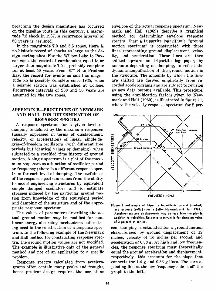
envelope of the actual response spectrum. New­mark and Hall (1969) describe a graphical method for determining envelope response spectra. First a tripartite logarithmic "ground motion spectrum" is constructed with three lines representing ground displacement, veloc­ity, and acceleration. These lines are then shifted upward on tripartite log paper, by amounts depending on damping, to reflect the dynamic amplification of the ground motion in the structure. The amounts by which the lines are shifted are derived empirically from re­corded accelerograms and are subject to revision as new data become available. This procedure, using the amplification factors give!l by New­mark and Hall (1969), is illustrated in figure 11, where the velocity response spectrum for 2 per-

<:) LaJ (/) -(/) LaJ

5•ot-~:...--~

>­.,_ (3 0 -J LaJ >

0.1 I FREQUENCY (CPS)

Figure I I.-Example of tripartite logarithmic grC'und (dashed) and response (solid) spectra (after Newmark and Hall, 1969). Accelerations and displacements may be read fr,,m the plot in addition to velocities. Response spectrum is for damping value of 2 percent of critical.

cent damping is estimated for a ground motion characterized by ground displacement of 12 inches, velocity of 16 inches per Sf'~ond, and acceleration of 0.33 g. At high and low frequen­cies, the response spectrum must theoretically equal the ground acceleration and dis"llacement, respectively ; this accounts for the slope that connects the 1.4 g and 0.33 g lines. The corres­ponding line at the low frequency side is off the graph to the left.

APPENDIX C-GROUND MOTION DATA

In studying the dependence of peak ground acceleration upon magnitude and distance to the causative fault, the strong-motion litera­ture was critically reviewed in an effort to com­pile data for which distances to the fault are most reliable, that is, most accurately deter­mined. By restricting the determination to use of only the most reliable data and further to data from a single event, a r-1

•5 to r-2

•0 depend­

ence of acceleration upon distance is clearly ob­served for distances as small as 10 km for mag­nitude 5, 20 km for magnitude 6, and less than 40 km for magnitude 7 (fig. 3). The importance of restricting the data set in determining the near-fault dependence of acceleration upon dis­tance is graphically demonstrated in figure 4, where the scatter in the entire data set is about an order of magnitude greater than the scatter for a single earthquake in figure 3. Because of the r-1

·5 to r-2

·0 attenuation of acceleration, the

location of the inferred fault is particularly crit­ical at small distances where the data are few.

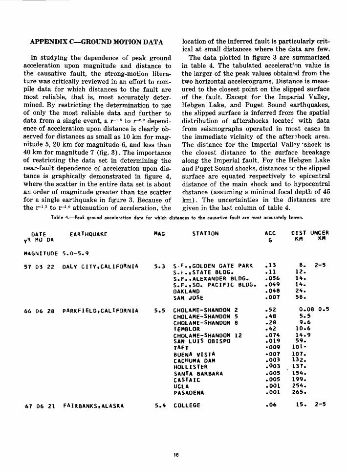
The data plotted in figure 3 are summarized in table 4. The tabulated accelerat~''>n value is the larger of the peak values obtain~d from the two horizontal accelerograms. Distance is meas­ured to the closest point on the slipped surface of the fault. Except for the Imperial Valley, Hebgen Lake, and Puget Sound earthquakes, the slipped surface is inferred from the spatial distribution of aftershocks located with data from seismographs operated in most cases in the immediate vicinity of the after~hock area. The distance for the Imperial Vall?.y ·shock is the closest distance to the surface breakage along the Imperial fault. For the Hebgen Lake and Puget Sound shocks, distances t<' the slipped surface are equated respectively to epicentral distance of the main shock and to hypocentral distance (assuming a minimal focal depth of 45 km). The uncertainties in the distances are given in the last column of table 4.

Table 4.-Peak ground acceleration data for which distances to the causative fault are most accurately known.

DATE EARTHQUAKE MAG STATION ACC OIST UNCER yR MO OA G KM KM

MAGNITUDE 5.0-5.9

57 03 22 DALY CITY,CALIFORNIA 5.3 S-f.,GOLOEN GATE PARK .13 a. 2-5 Se~.,STATE BLDG. • 11 12 • S.F.,ALEXANDER BLDG. • 056 14 • S.F.,SO. PACIFIC BLDG. • 049 14 • OAKLAND • 048 24 • SAN JOSE • 001 58 •

66 06 28 PARKFIELO,CALIFORNIA 5.5 CHOLAME-SHANOON 2 .52 o.oa 0.5 CHOLAME-SHANOON 5 .48 5.5 CHOLAME-SHANOON 8 .28 9.6 TEMBLOR .42 10·6 CHOLAME-SHANOON 12 .074 14.9 SAN LUIS OBISPO .019 59. TAFT •009 101• BUENA VISTA •001 107. CACHUMA DAM • 003 132 • HOLLISTER .003 137. SANTA BARBARA • 005 154 • CASTAIC • 005 199 • UCLA • 001 254 • PASADENA • 001 265 •

67 06 21 FAIRBANKS, ALASKA 5.4 COllEGE • 06 15 • 2-5

16

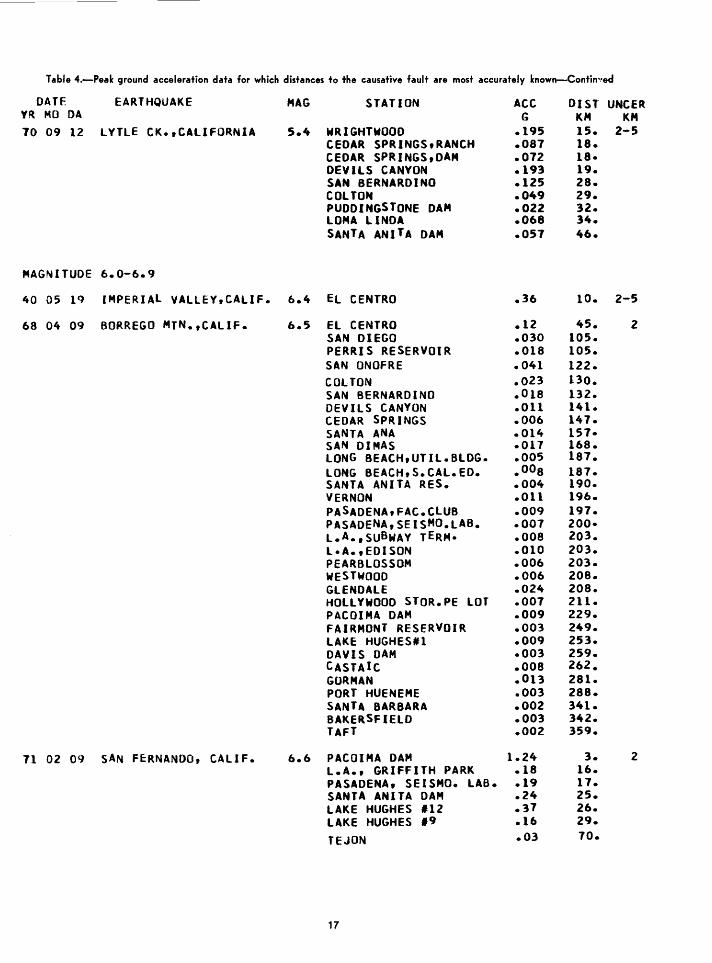
Table 4.-Peak ground acceleration data for which distances to the causative fault are most accurately known-Contin•1ed

OATF. EARTHQUAKE MAG STATION ACC DIST' UNCER YR MO DA G KM KM 70 09 12 LYTLE CK.,CALIFORNIA 5.4 WRIGHTWOOD .195 15. 2-5

CEDAR SPRINGStRANCH .087 18. CEDAR SPRINGS,DAM .072 18· DEVILS CANYON .193 19. SAN BERNARDINO .125 28. COLTON .049 29. PUDDINGSTONE DAM • 022 32 • LOMA LINDA • 068 34 • SANTA ANITA DAM .057 46.

MAGNITUDE 6.0-6.9

40 05 19 IMPERIAL VALLEY,CALIF. 6.4 EL CENTRO .36 10. 2-5

68 04 09 BORREGO MTN.,CALIF. 6.5 EL CENTRO .12 45. 2 SAN DIEGO • 030 105 • PERRIS RESERVOIR .018 105. SAN ONOFRE .041 122. COLTON • 023 130 • SAN BERNARDINO .018 132. DEVILS CANYON .011 141. CEDAR SPRINGS • 006 147 • SANTA ANA .014 157· SAN DIMAS ·017 168. LONG BEACH,UTIL.BLOG. .005 187. LONG BEACH,S.CAL.ED. .oo8 187. SANTA ANITA RES. • 004 190 • VERNON • 011 196 • PASAOENAtFAC.CLUB • 009 197 • PASAOENA,SEISMO.LAB. .oo1 200· L.A.,suBWAY TERM• • oo8 203 • l•A.,EDISON • 010 203 • PEARBLOSSOM • 006 203 • WESTWOOD • 006 208 • GLENDALE • 024 208 • HOLLYWOOD STOR.PE LOT • 007 211 • PACOIMA DAM • 009 229 • FAIRMONT RESERVOIR • 003 249 • LAKE HUGHESt1 • 009 253 • DAVIS DAM ·003 259. CASTAIC .008 262. GORMAN .013 281. PORT HUENEME .003 288. SANTA BARBARA • 002 341 • BAKERSFIELD • 003 342 • TAFT • 002 359 •

71 02 09 SAN FERNANDO, CALIF. 6.6 PACOIMA DAM 1.24 3. 2 L.A., GRIFFITH PARK • 18 16 • PASADENA, SEISMO. LAB. • 19 17 • SANTA ANITA DAM • 24 25 • LAKE HUGHES 112 .37 26. LAKE HUGHES 19 • 16 29 •

TEJON • 03 70 •

17

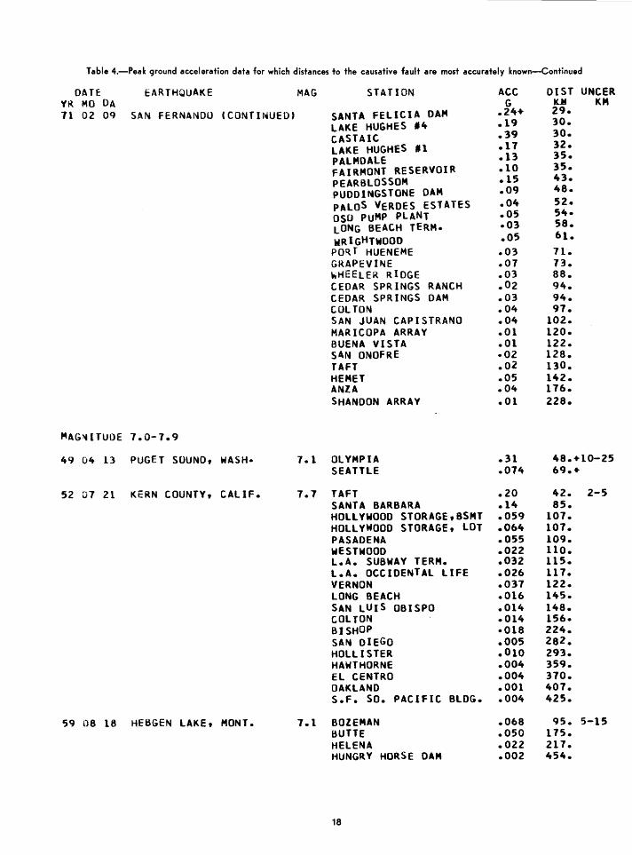
Table 4.-Peak ground acceleration data for which distances to the causative fault are most accurately known-Continued

DATE: YR MO DA 11 02 oq

EARTHQUAKE MAG STATION

SAN FERNANDO (CONTINUED) SANTA FELICIA DAM LAKE HUGHES 14 CASTAIC LAKE HUGHES t1 PALMDALE FAIRMONT RESERVOIR PEARBLOSSOM PUDDINGSTONE DAM PALOS VERDES ESTATES OSO PUMP PLANT tONG BEACH TERM· WRIGHTWOOD PORT HUENEME GRAPEVINE hHEELER RIDGE CEDAR SPRINGS RANCH CEDAR SPRINGS DAM COLTON SAN JUAN CAPISTRANO MARICOPA ARRAY BUENA VISTA SAN ONOFRE TAFT HEMET ANZA SHANDON ARRAY

MAG~ITUOE 7.0-7.9

49 04 13 PUGET SOUND, WASH•

52 07 21 KERN COUNTY, CALIF.

~9 08 18 HEBGEN LAKE, MONT.

1.1 OLYMPIA SEATTLE

7.7 TAFT SANTA BARBARA HOLLYWOOD STORAGE,BSMT HOLLYWOOD STORAGE, LOT PASADENA WESTWOOD L.A. SUBWAY TERM. L.A. OCCIDENTAL LIFE VERNON LONG BEACH SAN LUIS OBISPO COLTON BISHOP SAN DIEGO HOLLISTER HAWTHORNE EL CENTRO OAKLAND S.F. SO. PACIFIC BLDG.

7.1 BOZEMAN BUTTE HELENA HUNGRY HORSE DAM

18

ACC G

• 24+ • 19 • 39 • 17 • 13 • 10 • 15 • 09 • 04 .05 ·03 • 05 • 03 • 01 • 03 .02 .03 • 04 • 04 • 01 • 01 ·02 .02 • 05 .04 • 01

.31

.074

.20

.14

.059

.064 • 055 .022 .032 • 026 .037 • 016 .014 .014 ·018 .005 .010 • 004 .004 • 001 • 004

.068 • 050 • 022 • 002

DIST UNCER lUI KM 29 • 30 • 30 • 32 • 35 • 35 • 43 • 48 • 52 • 51t· 58. 61 • 71 • 73 • 88 • 94. 94. 97 •

102 • 120 • 122 • 128. 130. 142 • 176. 228 •

48.+10-25 69.+

42. 85.

107. 107 • 109. 110. 115. 117 • 122 • 145. 148. 156· 224. 282. 293 • 359. 370 • 407. 425 •

2-5

95. 5-15 175 • 217 • 454 •

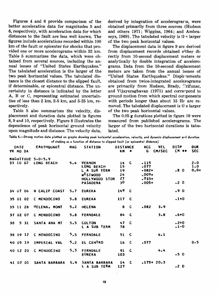
Figures 4 and 6 provide comparison of the better acceleration data for magnitudes 5 and 6, respectively, with acceleration data for which distances to the fault are less well known. The figures include accelerations recorded within 100 km of the fault or epicenter for shocks that pro­vided one or more accelerograms within 32 km. Table 5 summarizes the data, which were ob­tained from several sources, including the an­nual issues of "United States Earthquakes." The tabulated acceleration is the larger of the two peak horizontal values. The tabulated dis­tance is the closest distance to the slipped fault, if determinable, or epicentral distance. The un­certainty in distance is indicated by the letter A, B or C, representing estimated uncertain­ties of less than 2 km, 2-5 km, and 5-25 km, re­spectively.

Table 5 also summarizes the velocity, dis­placement and duration data pJotted in figures 8, 9 and 10, respectively. Figure 8 illustrates the dependence of peak horizontal ground velocity upon magnitude and distance. The velocity data,

derived by integration of ac~elerograns, were obtained primarily from three sources (Hudson and others 1971; Wiggins, 1964; and Ambra­seys, 1969). The tabulated velocity is tl'o. larger of the two peak horizontal values.

The displacement data in figure 9 ar~ derived from displacement records obtained e;ther di­rectly from 1 0-second displacement meters or analytically by double integration of accelero­grams. Data from the 10-second displacement meters are taken from the annual issues of "United States Earthquakes." Displr,~ements

obtained from twice-integrated accelerograms are primarily from Hudson, Brady, T'rifunac, and Vijayaraghavan (1971) and corre~pond to ground motion from which spectral cornponents with periods longer than about 15 H7. are re­moved. The tabulated displacement is tl'e larger of the two peak horizontal values.

The 0.05 g durations plotted in figure 10 were measured from published accelerograms. The larger of the two horizontal durations is tabu­lated.

Table 5.-Strong motion data plotted on graphs showing peak horizontal acceleration, velocity, and dynamic displacement ard duration

of shak_ing as a function of distance to slipped fault (or epicentral distance)

OlTE EARTHQUAKE MAG STATION DISTANCE ACC VEL OISP OUR YR MO DA KM • G CM/SEC CM •• SEC

MAGI~ITUOE 5·0-5.9 33 10 02 LONG BEACH 5.4 VERNON lit c .115 2·0

LONG BEACH 15 .011 1.0 L A SUB TERM 19 ·082+ .8 0 o.o+ wEsTwooo 24 .009+ HOLLYWOOD STOR 27 .033+ PASADENA 30 .005+ .2 0

34 07 06 N CALIF COAST 5.7 EUREKA 149 t .9 D

35 01 02 c MENDOCINO 5.8 EUREKA 117 c .1+0

35 11 28 HELENA, MONT 5.2 HELENA 8 c .082 3.9

37 02 07 C MENDOCINO 5.8 FERNDALE 84 c 3.8 .6+0

38 5 31 SANTA ANA MT 5.5 COLTON 47 c .2+0 L A SUB TERM 78 .1-0

38 09 12 C MENDOCINO 5.5 FERNDALE 51 c &.1

ItO 05 19 IMPERIAL VAL 5.2 EL CENTRO 16 c .077 0·5

ItO 12 20 C MENDOCINO 5.5 FERNDALE 91 c 4.4 EUREKA 103 .5 0

41 07 Ol SANTA BARBARA 5.9 SANTA BARBARA 14 c .175+ 20.3 L A SUB TERM 127 .2 D

19

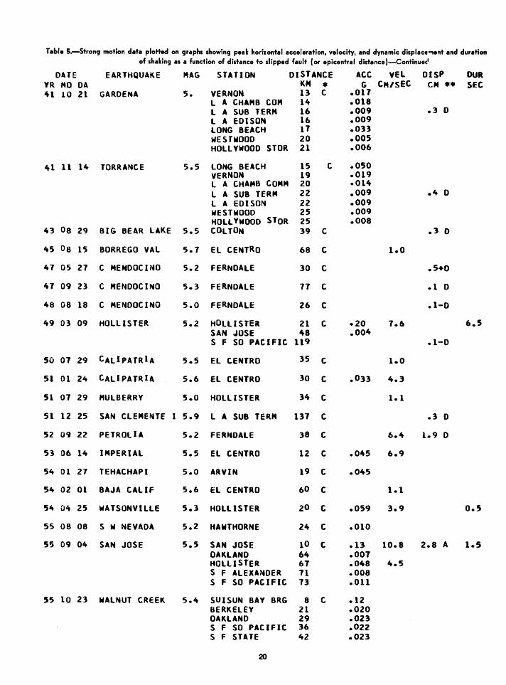
Table 5.-Strong motion data plotted on graphs showing peak horizontal acceleration, velocity, and dynamic displace"'''ent and duration of shaking as a function of distance fo slipped fault (or epicentral distance)-Continuec'

DATE EARTHQUAKE MAG STATION DISTANCE ACC VEL DISP OUR YR MO DA K·M • G CM/SEC CM ** SEC 4-1 10 21 GARDENA 5. VERNOM 13 c .017

l A CHAMB COM lit .018 L A SUB TERM 16 .009 .3 0 L A EDISON 16 .009 LONG BEACH 17 .013 WESTWOOD 20 .005 HOLLYWOOD STOR 21 .006

41 11 lit TORRANCE 5.5 lONG BEACH 15 t .050 VERNON 19 .019 L A CHAMB COMM 20 ·014 L A SUB TERM 22 .009 .It 0 l A EDISON 22 .009 WESTWOOD 25 .009 HOLLYWOOD STOR 25 .008

43 08 29 BIG BEAR lAKE 5.5 COLTON 39 c .3 0

45 os 15 BORREGO VAL 5.7 EL CENTRO 68 c 1.0

47 05 27 c MENDOCINO 5.2 FERNDALE 30 c .5+D

47 09 23 c MENDOCINO 5.3 FERNDALE 77 c .1 0

48 08 18 c MENDOCINO 5.0 FERNDALE 26 c .1-0

49 03 09 HOLLISTER 5.2 HOLLISTER 21 c ·20 7.6 6.5 SAN JOSE 48 .oo4 S F SO PACIFIC 119 .1-D

50 07 29 CALIPATRIA 5.5 EL CENTRO 35 c 1.0

51 01 24 CALIPATRIA 5.6 EL CENTRO 30 c .033 4.3

51 07 29 MULBERRY 5.0 HOLLISTER 34 c 1.1

51 12 25 SAN CLEMENTE I 5.9 L A SUB TERM 137 c .3 D

52 09 22 PETROLIA 5.2 FERNDALE 38 c 6.4 1.9 0

53 06 14 IMPERIAl 5.5 EL CENTRO 12 c .045 6.9

54 01 27 TEHACHAPI 5.0 ARVIN 19 c .045

54 02 01 BAJA CALIF 5.6 El CENTRO 60 c 1.1

54 04 25 WATSONVILLE 5.3 HOlliSTER 20 c .059 3.9 0.5

55 08 08 s w NEVADA 5.2 HAWTHORNE 24 c .010

55 09 04 SAN JOSE 5.5 SAN JOSE 10 t .13 10.8 2.8 A 1.5 OAKLAND 64 .007 HOLLISTER 67 • 048 4.5 S F ALEXANDER 71 .008 S F SO PACIFIC 73 .011

55 10 23 WALNUT CREEK 5.4 SUISUN BAY BRG 8 c .12 BERKELEY 21 .020 OAKLAND 29 .023 S F SO PACIFIC 36 .022 S F STATE 42 .023

20

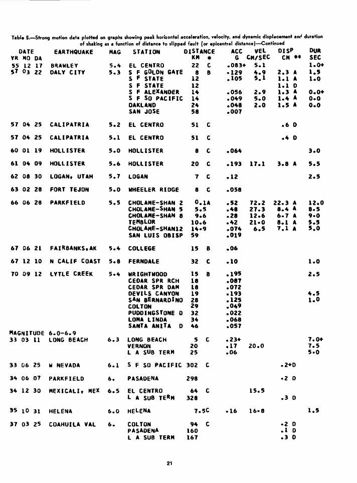
Table 5.-Strong motion data plotted on graphs showing peak horizontal acceleration, velocity, and dynamic displacement anc4 duration of shaking as a function of distance to slipped fault (or epicentral distance)-Continued

DATE EARTHQUAKE MAG STATION DISTANCE ACC veL DISP OUR YR MO DA KM • G CM/SEC CM •• sec 55 12 17 BltAWLEY 5.4 El CENTRO 22 c .083+ 5.1 1.0+ 57 03 22 DALY CITY 5.3 S F GDLDN GATE 8 B ·129 4.9 2.3 A 1.5

S F STATE 12 .105 5.1 1.1 A 1.0 S F STATE 12 1.1 D S F ALEXANDER lit .056 2.9 1.3 A o.o+ S F So PACIFIC lit .Oit9 5.0 1.it A o.o OAKLAND 2it .Oit8 2.0 1.5 A o.o SAN JOSE 58 .007

57 04 25 CALIPATRIA 5.2 El CENTRO 51 c .6 D

57 04 25 CALIPATRIA 5.1 EL CENTRO 51 c .4 D

60 01 19 HOLLISTER 5.0 HOLLISTER 8 c .064 3.0

61 04 09 HOLLISTER 5.6 HOLLISTER 20 c .193 17.1 3.8 A 5.5

62 08 30 LOGAN, UTAH 5.7 LOGAN 7 c .12 2.5

63 02 28 FORT TE-JON 5.0 WHEELER RIDGE 8 c .058

66 06 28 PARKFIELD 5.5 CHOLAME-SHAN 2 O.lA .52 72.2 22.3 A 12.0 CHOLAME-SHAN 5 5.5 .48 27.3 8.4 A 8·5 CHOLAME-SHAN 8 9.6 .21 12.6 6·7 A 9·0 TEMBLOR 10.6 .42 21·0 1.1 A 5.5 CHOLAME-SHAN12 14•9 .074 6.5 7.1 A 5.0 SAN lUIS DBISP 59 .019

67 06 21 FAIRBANKS,AK 5.4 COLLEGE 15 8 .06

67 12 10 N CALIF COAST 5.8 FERNDALE 32 c .10 1.0

70 09 12 LYTLE CREEK 5·4 WRIGHTWOOD 15 8 .195 2.5 CEDAR SPR RCH 18 .087 CEDAR SPR DAM 18 .072 DEVILS CANYON 19 .193 4.5 SAN BERNARDINO 28 .125 1.0 COLTON 29 .049 PUDDINGSTONE D 32 .022 LOMA LINDA 34 .068 SANTA ANITA D 46 .057

MAGNITUDE 6.0-6.9 33 03 11 LONG BEACH 6.3 LONG BEACH 5 c .23+ 7.0+

VERNON 20 .17 20.0 7.5 L A SUB TERM 25 .06 5·0

33 06 25 W NEVADA 6.1 S F SO PACIFIC 302 c .2+0

34 06 07 PARKFIELD 6. PASADENA 298 ·2 0

34 12 30 MEXICAllt MEX 6.5 EL CENTRO 64 c. 15.5 L A SUB TERM 328 .3 D

35 10 31 HELENA 6.0 HELENA 7.5C ·16 16•8 1.5

37 03 25 COAHUILA VAl 6. COLTON 94 c ·2 D PASADENA 160 .1 D L A SUB TERM 167 .3 D

21

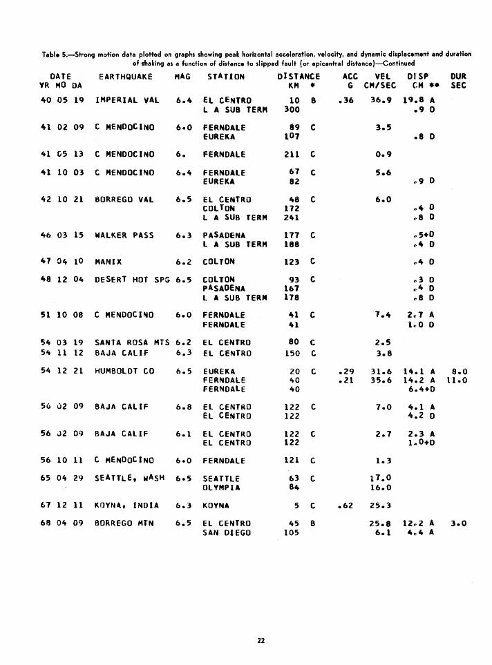
Table 5.-Strong motion data plotted on graphs showing peak horizontal acceleration, velocity, and dynamic displacement and duration of shaking as a function of distance to slipped fault (or epicentral distance )-Continued

DATE EARTHQUAKE MAG STATION DISTANCE Ate VEL DJSP DUR YR MO DA KM • G CM/SEC C:M •• SEC

ItO 05 19 IMPERIAL VAL 6.1t EL cENTRO 10 B .36 36.9 19.B A l A SUB TERM 300 .9 D

ltl 02 09 c MENDOCINO 6·0 FERNDALE 89 c 3.5 EUREKA 107 .a D

41 C5 13 c MENDOCINO 6. FERNDALE 211 c 0.9

41 10 0"3 c MENDOCINO 6.4 FERNDALE 67 c 5.6 EUREKA a2 ... 9 D

42 10 21 BORREGO VAL 6.5 El CENTRO 4a t 6.0 COLTON 172 .It D L A SUB TERM 241 ... a D

46 03 15 WALKER PASS 6.3 PASADENA 177 c .-.5+D l A SUB TERM 18a .-It 0

47 04 10 MANIX 6.2 COLTON 123 c ... It D

48 12 04 DESERT HOT SPG 6.5 COLTON 93 c .-3 D PASADENA 167 .,4 D L A SUB TERM 178 .. a D

51 10 08 C MENDOCI,..O 6.0 FERNDALE 41 c 7.4 2.-7 A FERNDALE 41 1.-0 0

54 03 19 SANTA ROSA MTS 6.2 EL CENTRO 80 c 2.5 54 11 12 BAJA CALIF 6.3 EL CENTRO 150 c 3.8

54 12 21 HUMBOLDT CO 6.5 EUREKA 20 c .29 31.6 14.1 A a.o FERNDALE 40 .21 35.6 14.2 A 11.0 FERNDALE 40 6.4+D

56 02 09 BAJA CALIF 6.8 EL CENTRO 122 c 7.0 4.1 A EL CENTRO 122 4.2 D

56 J2 09 BAJA CALIF 6.1 EL CENTRO 122 c 2.7 2.3 A EL CENTRO 122 1 .. 0+D

56 10 11 C MENDOCINO 6·0 FERNDALE 121 c 1.3

65 04 29 SEATTLE, WASH 6·5 SEATTLE 63 c 17.0 OLYMPIA 84 16.0

67 12 11 KOYN4t INDIA 6.3 KOYNA 5 c .62 25.3

68 04 09 BORREGO MTN 6.5 El CENTRO 45 8 25.a 12.-2 A 3.0 SAN DIEGO 105 6.1 4.-4 A

22

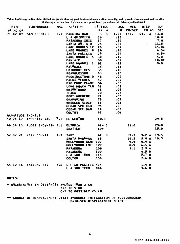
Table 5.-Strong motion data plotted on graphs showing peale horizontal acceleration, velocity, and dynamic displacement ar<'f duration of shaking as a function of distance to slipped fault (or epicentral distance)-Continued

O~TE yl( MO OA 71 02 09

EARTHQUAKE MAG STATION DISTANCE ACC VEl DISP OUR

SAN FERNA'iDO 6.6 PACOIMA DAM L A GRIFFITH PASADENA,SEIS SANTA ANITA 0 LAKE HUGHES 12 LAKE HUGHES 9 SANTA FELICIA LAKE HUGHES 4 CASTAIC

KM * G CM/SEC CM •~ SEC 3 8 1.24 115. 43. A 13.0

16 .18 10.0 17 .19 7.0 25 ·24 11.5 26 • 37 14.0+ 29 .16 4.5+ 29 .24 6.5+ 30 .19 4.0 30 • 39 ta.o+

1 32 .17 9·0 LAKE HUGHES PALMDALE FAIRMONT RES PEARBLOSSOM PUDDINGSTONE PALOS VERDES OSO PUMP PLANT LUNG BEACH TRM WRIGHTWOOD TEJON

35 ·13 35 .10 43 .15

0 48 .09

MAGNITUDE 7•0-7.9

PORT HUENEME GRAPEVINE WHEELER RIDGE CEDAR SPR RCH CEDAR SPR DAM COLTON

40 05 19 IMPfRIAl VAl 7.1 El CENTRO

49 04 l3 PUGET SND,WASH 7.1 OLYMPIA SEATTLE

52 07 21 KERN COUNTY 7.7 TAFT SANTA BARBARA HOllYWOOD BSMT HOLLYWOOD LOT PASADENA PASADENA L A SUB TERM COLTON

54 12 16 FALLON, NEV 1.0 S F SO PACIFIC L A SUB TERM

NOTES:

* UNCERTAINTY IN DISTANCE: A•LESS THAN 2 KM 8•2 TO 5 KM

52 .04 54 .05 58 .03 61 .05 10 .03 71 .03 73 .07 88 .03 94 • 02 94 .03 97 .04

10.8

48+ c 69+

42 8 85

107 107 109 109 115 156

404 584

C•5 TO POSSIBLY 25 KM

21.0

17·7 19.3 9.4 8.9 9.1

** SOURCE OF DISPLACEMENT DATA: A=DOUBLE INTEGRATION OF ACCELEROGRAM 0=10-SEC DISPLACEMENT METER

23

29·5

23·0 15.0

9·2 A 19.5 5.8 A 10.5 5.9 A 6.4 A 2.9 A 4.5 D 5.7 D 2.6 D

1.4 0 3.6 D

'tiGP 0 6 9 1• 3 54 -1 9 7 6