ground states of spinor bose-einstein condensate · bose-einstein condensatespinor bose-einstein...
TRANSCRIPT
Outline
Ground states of spinor Bose-Einstein condensate
Yongyong CaiBeijing Computational Science Research Center
joint with Weizhu Bao, W. Liu, Z. Wen, X. Wu, H. TianL. Wen, W. M. Liu, J. M. Zhang, and J. Hu
IMS, NUS, Oct. 4, 2019
1 / 36
Outline
1 Bose-Einstein condensate
2 Spinor Bose-Einstein condensates
3 Spin-1 BEC
4 Spin-2 BEC
2 / 36
Bose-Einstein condensate Spinor Bose-Einstein condensates Spin-1 BEC Spin-2 BEC
Bose-Einstein Condensation
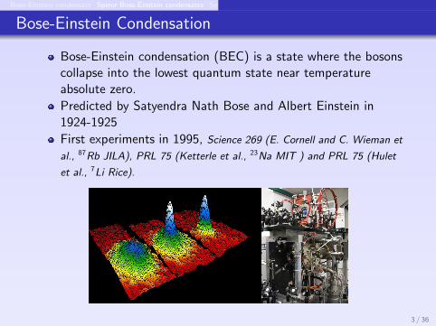
Bose-Einstein condensation (BEC) is a state where the bosonscollapse into the lowest quantum state near temperatureabsolute zero.
Predicted by Satyendra Nath Bose and Albert Einstein in1924-1925
First experiments in 1995, Science 269 (E. Cornell and C. Wieman et
al., 87Rb JILA), PRL 75 (Ketterle et al., 23Na MIT ) and PRL 75 (Hulet
et al., 7Li Rice).
3 / 36
Bose-Einstein condensate Spinor Bose-Einstein condensates Spin-1 BEC Spin-2 BEC
Spinor condensates
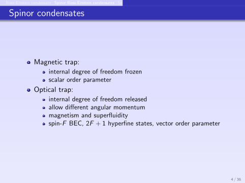
Magnetic trap:
internal degree of freedom frozenscalar order parameter
Optical trap:
internal degree of freedom releasedallow different angular momentummagnetism and superfluidityspin-F BEC, 2F + 1 hyperfine states, vector order parameter
4 / 36
Bose-Einstein condensate Spinor Bose-Einstein condensates Spin-1 BEC Spin-2 BEC
Pseudo spin-1/2 BEC
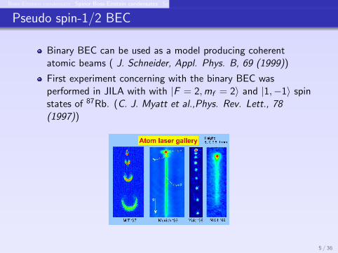
Binary BEC can be used as a model producing coherentatomic beams ( J. Schneider, Appl. Phys. B, 69 (1999))
First experiment concerning with the binary BEC wasperformed in JILA with with |F = 2,mf = 2〉 and |1,−1〉 spinstates of 87Rb. (C. J. Myatt et al.,Phys. Rev. Lett., 78(1997))
5 / 36
Bose-Einstein condensate Spinor Bose-Einstein condensates Spin-1 BEC Spin-2 BEC
Spin-orbit coupling in spin-1/2
Interaction of a particle’s spin with its motion
fine structure of Hydrogen
Electron: orbital angular momentum (generates magneticfield), interacts with the electron spin magnetic moment(internal Zeeman effect)
Crucial for quantum-Hall effects, topological insulators
Major experimental breakthrough in 2011, Lin et al. havecreated a SO coupled BEC, 85Rb: |↑〉 = |F = 1, mf = 0〉 and|↓〉 = |F = 1, mf = −1〉.SO coupling in cold atoms have been hot topics in recent years
6 / 36
Bose-Einstein condensate Spinor Bose-Einstein condensates Spin-1 BEC Spin-2 BEC
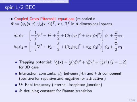
spin-1/2 BEC
• Coupled Gross-Pitaevskii equations (re-scaled):Ψ := (ψ1(x, t), ψ2(x, t))T , x ∈ Rd in d dimensional spaces
i∂tψ1 =
[−1
2∇2 + V1 +
δ
2+ (β11|ψ1|2 + β12|ψ2|2)
]ψ1 +
Ω
2ψ2,
i∂tψ2 =
[−1
2∇2 + V2 −
δ
2+ (β21|ψ1|2 + β22|ψ2|2)
]ψ2 +
Ω
2ψ1,
Trapping potential: Vj(x) = 12 (γ2
xx2 + γ2
yy2 + γ2
z z2) (j = 1, 2)
for 3D case
Interaction constants: βjl between j-th and l-th component(positive for repulsive and negative for attractive )
Ω: Rabi frequency (internal Josephson junction)
δ: detuning constant for Raman transition
7 / 36

Bose-Einstein condensate Spinor Bose-Einstein condensates Spin-1 BEC Spin-2 BEC
Conserved quantities
Mass:
N(t) := ‖Ψ(·, t)‖2 =
∫
Rd
[|ψ1(x, t)|2+|ψ2(x, t)|2]dx ≡ N(0) = 1,
Energy per particle
E (Ψ) =
∫
Rd
[ 2∑
j=1
(1
2|∇ψj |2 + Vj(x)|ψj |2
)+δ
2
(|ψ1|2 − |ψ2|2
)
+ Ω Re(ψ1ψ2) +β11
2|ψ1|4 +
β22
2|ψ2|4 + β12|ψ1|2|ψ2|2
]dx
Ground state patterns
8 / 36
Bose-Einstein condensate Spinor Bose-Einstein condensates Spin-1 BEC Spin-2 BEC
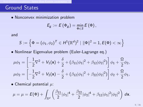
Ground States
• Nonconvex minimization problem
Eg := E (Φg ) = minΦ∈S
E (Φ) ,
and
S :=
Φ = (φ1, φ2)T ∈ H1(Rd)2 | ‖Φ‖2 = 1,E (Φ) <∞
• Nonlinear Eigenvalue problem (Euler-Lagrange eq.)
µφ1 =
[−1
2∇2 + V1(x) +
δ
2+ (β11|φ1|2 + β12|φ2|2)
]φ1 +
Ω
2φ2,
µφ2 =
[−1
2∇2 + V2(x)− δ
2+ (β12|φ1|2 + β22|φ2|2)
]φ2 +
Ω
2φ1,
• Chemical potential µ:
µ = µ = E (Φ) +
∫
Rd
(β11
2|φ1|4 +
β22
2|φ2|4 + β12|φ1|2|φ2|2
)dx.
9 / 36
Bose-Einstein condensate Spinor Bose-Einstein condensates Spin-1 BEC Spin-2 BEC
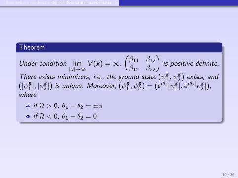
Theorem
Under condition lim|x |→∞
V (x) =∞,
(β11 β12
β12 β22
)is positive definite.
There exists minimizers, i.e., the ground state (ψg1 , ψ
g2 ) exists, and
(|ψg1 |, |ψ
g2 |) is unique. Moreover, (ψg
1 , ψg2 ) = (e iθ1 |ψg
1 |, e iθ2|ψg2 |),
where
if Ω > 0, θ1 − θ2 = ±πif Ω < 0, θ1 − θ2 = 0
10 / 36
Bose-Einstein condensate Spinor Bose-Einstein condensates Spin-1 BEC Spin-2 BEC
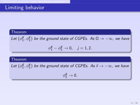
Limiting behavior
Theorem
Let (φg1 , φg2 ) be the ground state of CGPEs. As Ω→ −∞, we have
φg1 − φg2 → 0, j = 1, 2.
Theorem
Let (φg1 , φg2 ) be the ground state of CGPEs. As δ → −∞, we have
φg2 → 0.
11 / 36
Bose-Einstein condensate Spinor Bose-Einstein condensates Spin-1 BEC Spin-2 BEC
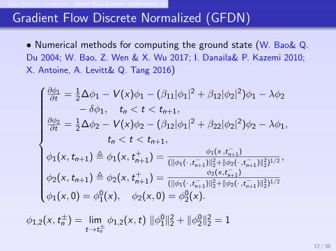
Gradient Flow Discrete Normalized (GFDN)
• Numerical methods for computing the ground state (W. Bao& Q.
Du 2004; W. Bao, Z. Wen & X. Wu 2017; I. Danaila& P. Kazemi 2010;
X. Antoine, A. Levitt& Q. Tang 2016)
∂φ1∂t = 1
2 ∆φ1 − V (x)φ1 − (β11|φ1|2 + β12|φ2|2)φ1 − λφ2
− δφ1, tn < t < tn+1,∂φ2∂t = 1
2 ∆φ2 − V (x)φ2 − (β12|φ1|2 + β22|φ2|2)φ2 − λφ1,
tn < t < tn+1,
φ1(x , tn+1) , φ1(x , t+n+1) =
φ1(x ,t−n+1)
(‖φ1(· ,t−n+1)‖22+‖φ2(· ,t−n+1)‖2
2)1/2 ,
φ2(x , tn+1) , φ2(x , t+n+1) =
φ2(x ,t−n+1)
(‖φ1(· ,t−n+1)‖22+‖φ2(· ,t−n+1)‖2
2)1/2
φ1(x , 0) = φ01(x), φ2(x , 0) = φ0
2(x).
φ1,2(x , t±n ) = limt→t±n
φ1,2(x , t) ‖φ01‖2
2 + ‖φ02‖2
2 = 1
12 / 36
Bose-Einstein condensate Spinor Bose-Einstein condensates Spin-1 BEC Spin-2 BEC
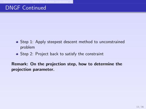
DNGF Continued
Step 1: Apply steepest descent method to unconstrainedproblem
Step 2: Project back to satisfy the constraint
Remark: On the projection step, how to determine theprojection parameter.
13 / 36
Bose-Einstein condensate Spinor Bose-Einstein condensates Spin-1 BEC Spin-2 BEC
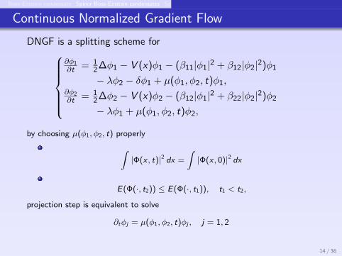
Continuous Normalized Gradient Flow
DNGF is a splitting scheme for
∂φ1∂t = 1
2 ∆φ1 − V (x)φ1 − (β11|φ1|2 + β12|φ2|2)φ1
− λφ2 − δφ1 + µ(φ1, φ2, t)φ1,∂φ2∂t = 1
2 ∆φ2 − V (x)φ2 − (β12|φ1|2 + β22|φ2|2)φ2
− λφ1 + µ(φ1, φ2, t)φ2,
by choosing µ(φ1, φ2, t) properly∫|Φ(x , t)|2 dx =
∫|Φ(x , 0)|2 dx
E(Φ(·, t2)) ≤ E(Φ(·, t1)), t1 < t2,
projection step is equivalent to solve
∂tφj = µ(φ1, φ2, t)φj , j = 1, 2
14 / 36

Bose-Einstein condensate Spinor Bose-Einstein condensates Spin-1 BEC Spin-2 BEC
15 / 36
Bose-Einstein condensate Spinor Bose-Einstein condensates Spin-1 BEC Spin-2 BEC
16 / 36
Bose-Einstein condensate Spinor Bose-Einstein condensates Spin-1 BEC Spin-2 BEC
Phase separation
Property Let β12 → +∞, the phase of two components of theground state Φg = (φg1 , φ
g2 )T will be segregated, i.e. Φg will
converge to a state such that φg1 · φg2 = 0.
17 / 36
Bose-Einstein condensate Spinor Bose-Einstein condensates Spin-1 BEC Spin-2 BEC
Phase separation
Repulsive interactions only:
E (φ1, φ2) =
∫1
2|∇φ1|2 +
1
2|∇φ2|2 +
β11
2|φ1|4
+β22
2|φ2|4 + β12|φ1|2|φ2|2
Homogeneous case: β11β22 ≥ β212 mixed; otherwise separated
Nonhomogeneous case?
18 / 36
Bose-Einstein condensate Spinor Bose-Einstein condensates Spin-1 BEC Spin-2 BEC
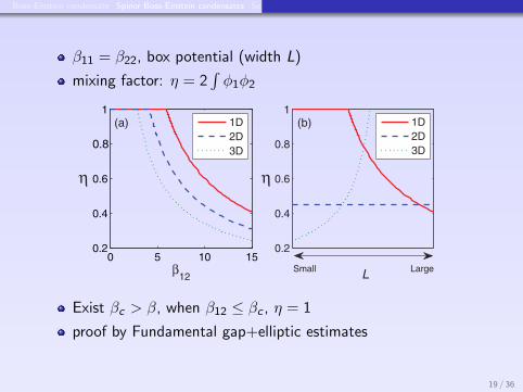
β11 = β22, box potential (width L)
mixing factor: η = 2∫φ1φ2
CONTROLLING PHASE SEPARATION OF A TWO- . . . PHYSICAL REVIEW A 85, 043602 (2012)
0 5 10 150.2
0.4
0.6
0.8
1
β12
1D2D3D
0.2
0.4
0.6
0.8
1
1D2D3D
Small Large
(a) (b)
L
η η
FIG. 1. (Color online) (a) The overlap factor η as a function of thereduced parameter β12 [see Eq. (6)] in different dimensions (infinitelydeep square well potential case g11 = g22 = 0). Note that for all valuesof d there exists a critical value βc
12 = 0, below which η attains itsmaximal possible value 1. (b) A schematic plot of η vs the width ofthe square well in different dimensions. Note the counterintuitive factthat in the three-dimensional case (d = 3) the stronger we squeezethe system (the smaller L is) the stronger phase separation is (thesmaller η is).
kinetic terms dominate and phase separation is suppressedregardless of the condition (1). The two-dimensional caseis another story. The parameter L simply drops out in thecurly braces. It is no use to adjust the width of the well toenhance the importance of the kinetic energy or the interactionenergy relatively. The kinetic and interaction energies shouldbe treated on an equal footing, which means the analysisleading to criterion (1) may be invalid.
We have checked all these predictions numerically. Notethat on the problem of phase separation, the intracomponentinteractions are on the same side as the kinetic energy—theyboth try to delocalize the condensates. Therefore, to highlightthe effect of kinetic energy, we shall set g11 = g22 = 0 (β11 =β22 = 0) so that the kinetic energy is the only element actingagainst phase separation. As we shall see below, this specialcase also admits a simple analytical analysis.
We have solved the ground state of the system in alldimensions for a given value of β12 [16]. The overlap factorη is plotted versus β12 in Fig. 1(a). We observe that inall dimensions there exists a critical value of β12 (denotedas βc
12), below which the two condensates wave functionsare equal (η = 1). That is, for β12 βc
12, phase separationis completely suppressed. Above the critical value, phaseseparation develops (η < 1) as β12 increases, but is still greatlysuppressed for a wide range of value of β12. It should bestressed that though in Fig. 1(a) the curves of η − β12 arequalitatively similar to each another for all values of d (theplateau of η = 1 is always located in the direction of β12 → 0),the curves of η − L will be quite different. The reason is thatβ12 ∝ L2−d . Figure 1(b) is a schematic plot of η versus L in allthree cases. It shows that η as a function of L is monotonicallydecreasing, constant, and monotonically increasing in one,two, and three dimensions, respectively. This means that tosuppress phase separation, in one dimension we should tightenthe confinement, in three dimensions we should loosen theconfinement, while in two dimensions it is useless to changethe confinement. Overall, Fig. 1 confirms the initial conjecturethat kinetic energy can suppress phase separation.
In hindsight, we can actually understand why phase separa-tion can be suppressed in the limits of L → 0 in one dimensionand L → ∞ in three dimensions. Consider two differentconfigurations. The first one is a phase-separated one—the twocondensates occupy the left and right halves of the containerseparately. The second one is a phase-mixed one—the twocondensates both occupy the whole space available and thusoverlap significantly. Compared with the first configuration,the second one costs more intercomponent interaction energy,which is on the order of L−d , but saves more kinetic energy,which is on the order of L−2. The second configuration (phasemixed) is more economical in energy in the limit of L → 0and L → ∞, in the cases of d = 1 and d = 3, respectively.The case of d = 2 is more subtle and which configuration winsdepends on parameters other than L.
A remarkable fact revealed in Fig. 1, but not so obvious inour arguments, is that in the symmetric case with β11 = β22 =0, η = 1 for β12 βc
12, which is on the order of unity. This isa stronger fact than η → 1 as β12 → 0 as we argued. Actually,the general observation is that for β11 = β22 > 0, η = 1 forβ12 smaller than its critical value βc
12, which is larger than β11.This fact has rich meanings. On the one hand, it demonstratesthat the kinetic energy is very effective—phase separation canbe completely suppressed by it even if β12 > β11 = β22, that is,when (1) is satisfied. On the other hand, it strongly indicatesthat as β12 crosses the critical value, the system undergoesa second-order phase transition which can fit in the Landauformalism. The picture is that the exchange symmetry φ1 ↔ φ2
of the energy functional (5) is preserved for β12 < βc12, but is
spontaneously broken as β12 surpasses βc12.
We have been able to prove the first point rigorously onthe mathematical level (see Appendix A). However, it is alsodesirable to develop a physical understanding of the two points.This can be achieved by studying a two-component BEC in adouble-well potential (see Appendix B) or using a variationalapproach [17]. We note that in the limit of β12 → 0, φ1,2
both converge to the (nondegenerate) ground state of a singleparticle in the [−1/2, + 1/2]d infinitely deep square well.As β12 is turned on, the two wave functions are deformedand excited states mix in. Because the energies of the excitedstates grow up quadratically, we cut off at the first excitedlevel and take the following ansatz for the two condensatewave functions:
φ1 = c0ϕ0 + c1ϕ1, φ2 = c0ϕ0 − c1ϕ1. (7)
Here ϕ0 is the ground state, while ϕ1 is one of the possiblydegenerate first excited states. The coefficients c0,1 are real andsatisfy the normalization condition c2
0 + c21 = 1. Obviously,
complete phase mixing would correspond to c1 = 0, whilepartial phase separation to c1 = 0. Our numerical simulationsindicate that (this is also supported by the variational approachitself, see Appendix C) in the two-dimensional case, whenphase separation occurs, the two condensates are shifted eitheralong x or y direction; in the three-dimensional case, whenphase separation occurs, the two condensates are shifted eitheralong x or y or z direction. This fact motivates us to chooseϕ1 in the following form:
d = 1 : ϕ1 = w1(x), (8a)
d = 2 : ϕ1 = w0(x)w1(y) or w1(x)w0(y), (8b)
043602-3
Exist βc > β, when β12 ≤ βc , η = 1
proof by Fundamental gap+elliptic estimates
19 / 36
Bose-Einstein condensate Spinor Bose-Einstein condensates Spin-1 BEC Spin-2 BEC
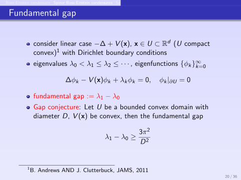
Fundamental gap
consider linear case −∆ + V (x), x ∈ U ⊂ Rd (U compactconvex)1 with Dirichlet boundary conditions
eigenvalues λ0 < λ1 ≤ λ2 ≤ · · · , eigenfunctions φk∞k=0
∆φk − V (x)φk + λkφk = 0, φk |∂U = 0
fundamental gap := λ1 − λ0
Gap conjecture: Let U be a bounded convex domain withdiameter D, V (x) be convex, then the fundamental gap
λ1 − λ0 ≥3π2
D2
1B. Andrews AND J. Clutterbuck, JAMS, 201120 / 36
Bose-Einstein condensate Spinor Bose-Einstein condensates Spin-1 BEC Spin-2 BEC
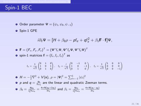
Spin-1 BEC
Order parameter Ψ = (ψ1, ψ0, ψ−1)
Spin-1 GPE
i∂tΨ = [H + β0ρ− pfz + qf2z + β1F · f]Ψ,
F = (Fx ,Fy ,Fz)T = (Ψ∗fxΨ,Ψ∗fyΨ,Ψ∗fzΨ)T
spin-1 matrices f = (fx , fy , fz)T as
fx =1√
2
0 1 01 0 10 1 0
, fy =i√
2
0 −1 01 0 −10 1 0
, fz =1√
2
1 0 00 0 00 0 −1
H = − 12∇2 + V (x), ρ = |Ψ|2 =
∑1l=−1 |ψl |2
p and q = q0~ωs
are the linear and quadratic Zeeman terms.
β0 = Nc0x3s ~ωs
= 4πN(a0+2a2)3xs
and β1 = Nc2x3s ~ωs
= 4πN(a2−a0)3xs
21 / 36
Bose-Einstein condensate Spinor Bose-Einstein condensates Spin-1 BEC Spin-2 BEC
Energy and ground states
Fx = 1√2
[ψ1ψ0 + ψ0(ψ1 + ψ−1) + ψ−1ψ0
], Fy = i√
2
[−ψ1ψ0 + ψ0(ψ1 − ψ−1) + ψ−1ψ0
],
Fz = |ψ1|2 − |ψ−1|2
Energy:
E(Ψ(·, t)) =
∫Rd
1∑
l=−1
(1
2|∇ψl |
2 + (V (x)− pl + ql2)|ψl |2)
+β0
2|Ψ|4 +
β1
2|F|2
dx
Mass constraint N(Ψ(·, t)) := ‖Ψ(·, t)‖2 =∫Rd∑
l=−1,0,1 |ψl (x, t)|2 dx = N(Ψ(·, 0)) = 1
Magnetization (M ∈ [−1, 1]) M(Ψ(·, t)) :=∫Rd∑
l=−1,0,1 l|ψl (x, t)|2 dx = M(Ψ(·, 0)) = M
Ground state- Find(
Φg ∈ SM)
such that Eg := E(
Φg)
= minΦ∈SM E (Φ)
SM =
Φ = (φ1, φ0, φ−1)T | ‖Φ‖ = 1,
∫Rd
[|φ1(x)|2 − |φ−1(x)|2
]dx = M, E(Φ) <∞
.
22 / 36
Bose-Einstein condensate Spinor Bose-Einstein condensates Spin-1 BEC Spin-2 BEC
Properties
Quadratic Zeeman q = 0
Ferromagnetic system-spin-dependent interacton β1 < 0
Single mode approximation.φj identical up to a constant factor
Anti-ferromagnetic system-spin-dependent interacton β1 > 0
φ0 = 0
|F|2 = (|φ1|2 − |φ−1|2)2 + 2|φ0|2(|φ1|2 + |φ−1|2)− 4Re(φ20φ1φ−1)
Fx = Fy 6= 0: ferromagnetic; Fx = Fy = 0: anti-ferromagnetic
23 / 36
Bose-Einstein condensate Spinor Bose-Einstein condensates Spin-1 BEC Spin-2 BEC
Mathematical results
Theorem
Existence: lim|x|→∞
V (x) = +∞, M ∈ (−1, 1), β0 ≥ 0 and β0 + β1 ≥ 0, there
exists ground state Φg = (φg1 , φ
g0 , φ
g−1) ∈ SM
q = 0 and β1 < 0, ferromagnetic: φgl = e iθlαlφg
(θ1 + θ−1 − 2θ0 = (2k + 1)π, α1 = 1+M2
, α−1 = 1−M2
, α0 =√
1−M2
2
q < 0 and β1 > 0, anti-ferromagnetic: φg0 = 0, and Φg = (φg
1 , φg−1)T is a
minimizer of the pseudo spin-1/2 system
24 / 36

Bose-Einstein condensate Spinor Bose-Einstein condensates Spin-1 BEC Spin-2 BEC
Numerical methods
Normalized Gradient Flow:
∂tφ1 =
[1
2∇2 − V (x)− (β0 + β1)(|φ1|
2 + |φ0|2)− (β0 − β1)|φ−1|
2]φ1 − β1φ−1φ
20 + [µΦ(t) + λΦ(t)]φ1
∂tφ0 =
[1
2∇2 − V (x)− (β0 + β1)(|φ1|
2 + |φ−1|2)− β0|φ0|
2]φ0 − 2β1φ−1 φ0φ1 + µΦ(t) φ0
∂tφ−1 =
[1
2∇2 − V (x)(β0 + β1)(|φ−1|
2 + |φ0|2)− (β0 − β1)|φ1|
2]φ−1 − β1φ
20 φ1 + [µΦ(t)− λΦ(t)]φ−1
• Gradient flow part (imaginary time spin-1 GPE)+projection (Lagrange
multipliers)//Gradient flow part (imaginary time spin-1 GPE+Lagrange
multipliers) + projection (Lagrange part)
• For projection constants: φl(x, t+n+1) = σlφl(x, t
−n+1) (l = ±1, 0), two
equations from Mass and Magnetization constraints, from
∂tφl(x, t) = [µΦ(t) + lλΦ(t)]φl(x, t), an additional equation σ1σ−1 = σ20 .
(quadrattic equation to be solved for σl)
25 / 36
Bose-Einstein condensate Spinor Bose-Einstein condensates Spin-1 BEC Spin-2 BEC
Numerical results
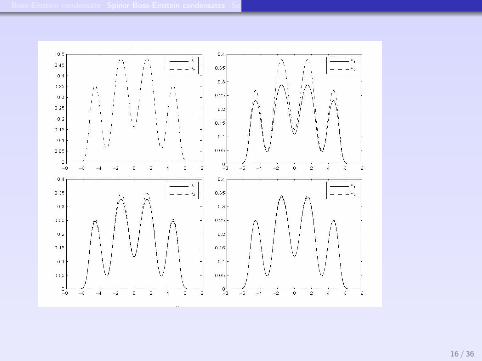
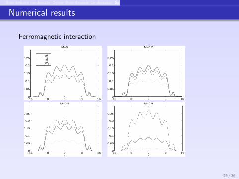
Ferromagnetic interactionCONTENTS 41
−16 −8 0 8 160
0.05
0.1
0.15
0.2
0.25
M=0
φ1g
φ0g
φ−1g
−16 −8 0 8 160
0.05
0.1
0.15
0.2
0.25
M=0.2
−16 −8 0 8 160
0.05
0.1
0.15
0.2
0.25
x
M=0.5
−16 −8 0 8 160
0.05
0.1
0.15
0.2
0.25
x
M=0.9
Figure 4.1: Wave functions of the ground state, i.e., φg1(x) (dashed line), φ
g0(x) (solid line),
and φg−1(x) (dotted line), of 87Rb in Example 4.1 case I with a fixed number of particles
N=104 for different magnetizations M=0,0.2,0.5,0.9 in an optical lattice potential.
Example 4.1. To show the ground states of the spin-1 BEC, we take d = 1, p = q = 0,V(x)=x2/2+25sin2(πx
4
)in (4.2). Two different types of interaction strengths are chosen
as
• Case I. For 87Rb with dimensionless quantities in (4.2) used as β0 = 0.0885N, andβ1 =−0.00041N with N the total number of atoms in the condensate and the di-mensionless length unit as =2.4116×10⁻⁶ [m] and time unit ts =0.007958 [s].
• Case II. For 23Na with dimensionless quantities in (4.2) used as β0 = 0.0241N, andβ1=0.00075N, with N the total number of atoms in the condensate and the dimen-sionless length unit as =4.6896×10⁻⁶ [m] and time unit ts =0.007958 [s].
The ground states are computed numerically by the backward Euler sine pseudospec-tral method presented in [27]. Figure 4.1 shows the ground state solutions of 87Rb in caseI with N=104 for different magnetizations M. Figure 4.2 shows similar results for 23Nain case II.
26 / 36
Bose-Einstein condensate Spinor Bose-Einstein condensates Spin-1 BEC Spin-2 BEC
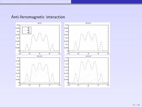
Anti-ferromagnetic interaction42 CONTENTS
−12 −6 0 6 12
0
0.05
0.1
0.15
0.2
0.25
0.3
0.35
0.4M=0
φ1g
φ0g
φ−1g
−12 −6 0 6 12
0
0.05
0.1
0.15
0.2
0.25
0.3
0.35
0.4M=0.2
−12 −6 0 6 12
0
0.05
0.1
0.15
0.2
0.25
0.3
0.35
0.4
x
M=0.5
−12 −6 0 6 12
0
0.05
0.1
0.15
0.2
0.25
0.3
0.35
0.4
x
M=0.9
Figure 4.2: Wave functions of the ground state, i.e., φg1(x) (dashed line), φ
g0(x) (solid
line), and φg−1(x) (dotted line), of 23Na in Example 4.1 case II with N = 104 for different
magnetizations M=0,0.2,0.5,0.9 in an optical lattice potential.
For the cases when q = 0 in Theorems 4.2&4.3, the minimization problem (4.9) canbe reduced to a single component and a two component system, respectively, where thenumerical methods could be simplified [20].
We remark here that there is another type of ground state of the spin-1 BEC, especiallywith an Ioffe-Pritchard magnetic field B(x), in the literatures [20, 70], which is defined asthe minimizer of the energy functional subject to the conservation of total mass:
Find(Φg∈S
)such that
Eg :=E(Φg)=min
Φ∈SE(Φ), (4.26)
where the nonconvex set S is defined as
S=
Φ=(φ1,φ0,φ−1)T | ‖Φ‖=1, E(Φ)<∞
. (4.27)
For the analysis and numerical simulation of this type of the ground state of spin-1 BEC,we refer to [20,57,70] and references therein. In addition, when there is no Ioffe-Pritchard
27 / 36
Bose-Einstein condensate Spinor Bose-Einstein condensates Spin-1 BEC Spin-2 BEC
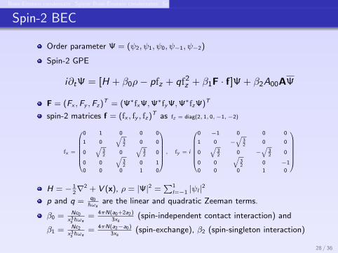
Spin-2 BEC
Order parameter Ψ = (ψ2, ψ1, ψ0, ψ−1, ψ−2)
Spin-2 GPE
i∂tΨ = [H + β0ρ− pfz + qf2z + β1F · f]Ψ + β2A00AΨ
F = (Fx ,Fy ,Fz)T = (Ψ∗fxΨ,Ψ∗fyΨ,Ψ∗fzΨ)T
spin-2 matrices f = (fx , fy , fz)T as fz = diag(2, 1, 0,−1,−2)
fx =
0 1 0 0 0
1 0√
32
0 0
0√
32
0√
32
0
0 0√
32
0 1
0 0 0 1 0
, fy = i
0 −1 0 0 0
1 0 −√
32
0 0
0√
32
0 −√
32
0
0 0√
32
0 −1
0 0 0 1 0
H = − 12∇2 + V (x), ρ = |Ψ|2 =
∑1l=−1 |ψl |2
p and q = q0~ωs
are the linear and quadratic Zeeman terms.
β0 = Nc0x3s ~ωs
= 4πN(a0+2a2)3xs
(spin-independent contact interaction) and
β1 = Nc2x3s ~ωs
= 4πN(a2−a0)3xs
(spin-exchange), β2 (spin-singleton interaction)
28 / 36
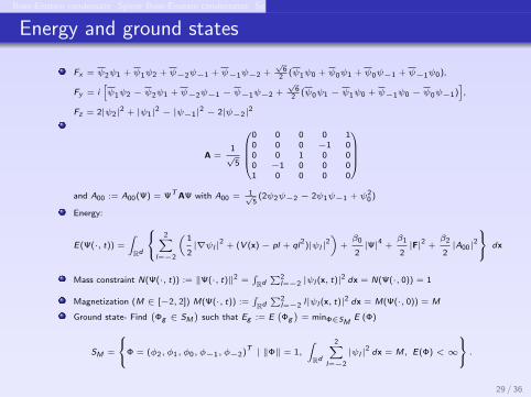
Bose-Einstein condensate Spinor Bose-Einstein condensates Spin-1 BEC Spin-2 BEC
Energy and ground states
Fx = ψ2ψ1 + ψ1ψ2 + ψ−2ψ−1 + ψ−1ψ−2 +√
62
(ψ1ψ0 + ψ0ψ1 + ψ0ψ−1 + ψ−1ψ0),
Fy = i[ψ1ψ2 − ψ2ψ1 + ψ−2ψ−1 − ψ−1ψ−2 +
√6
2(ψ0ψ1 − ψ1ψ0 + ψ−1ψ0 − ψ0ψ−1)
],
Fz = 2|ψ2|2 + |ψ1|2 − |ψ−1|2 − 2|ψ−2|2
A =1√
5
0 0 0 0 10 0 0 −1 00 0 1 0 00 −1 0 0 01 0 0 0 0
and A00 := A00(Ψ) = ΨTAΨ with A00 = 1√
5(2ψ2ψ−2 − 2ψ1ψ−1 + ψ2
0 )
Energy:
E(Ψ(·, t)) =
∫Rd
2∑
l=−2
(1
2|∇ψl |
2 + (V (x)− pl + ql2)|ψl |2)
+β0
2|Ψ|4 +
β1
2|F|2 +
β2
2|A00|
2
dx
Mass constraint N(Ψ(·, t)) := ‖Ψ(·, t)‖2 =∫Rd∑2
l=−2 |ψl (x, t)|2 dx = N(Ψ(·, 0)) = 1
Magnetization (M ∈ [−2, 2]) M(Ψ(·, t)) :=∫Rd∑2
l=−2 l|ψl (x, t)|2 dx = M(Ψ(·, 0)) = M
Ground state- Find(
Φg ∈ SM)
such that Eg := E(
Φg)
= minΦ∈SM E (Φ)
SM =
Φ = (φ2, φ1, φ0, φ−1, φ−2)T | ‖Φ‖ = 1,
∫Rd
2∑l=−2
|ψl |2 dx = M, E(Φ) <∞
.29 / 36
Bose-Einstein condensate Spinor Bose-Einstein condensates Spin-1 BEC Spin-2 BEC
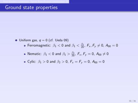
Ground state properties
Uniform gas, q = 0 (cf. Ueda 09)
Ferromagnetic: β1 < 0 and β1 <β2
20 , Fx ,Fy 6= 0, A00 = 0
Nematic: β1 < 0 and β1 >β2
20 , Fx ,Fy = 0, A00 6= 0
Cylic: β1 > 0 and β2 > 0, Fx = Fy = 0, A00 = 0
30 / 36
Bose-Einstein condensate Spinor Bose-Einstein condensates Spin-1 BEC Spin-2 BEC
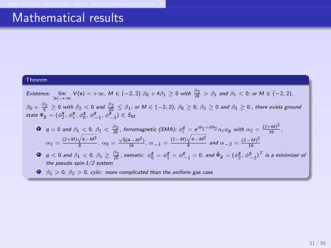
Mathematical results
Theorem
Existence: lim|x|→∞
V (x) = +∞, M ∈ (−2, 2) β0 + 4β1 ≥ 0 withβ220> β1 and β1 < 0; or M ∈ (−2, 2),
β0 +β25≥ 0 with β2 < 0 and
β220≤ β1; or M ∈ (−2, 2), β0 ≥ 0, β1 ≥ 0 and β2 ≥ 0., there exists ground
state Φg = (φg2 , φ
g1 , φ
g0 , φ
g−1, φ
g−2) ∈ SM
q = 0 and β1 < 0, β1 <β220
, ferromagnetic (SMA): φgl
= e iθ1+ilθ2αlφg with α2 =(2+M)2
16,
α1 =(2+M)
√4−M2
8, α0 =
√6(4−M2)
16, α−1 =
(2−M)
√4−M2
8and α−2 =
(2−M)2
16
q < 0 and β1 < 0, β1 ≥β220
, nematic: φg0 = φ
g1 = φ
g−1 = 0, and Φg = (φ
g2 , φ
g−2)T is a minimizer of
the pseudo spin-1/2 system
β1 > 0, β2 > 0, cylic: more complicated than the uniform gas case
31 / 36
Bose-Einstein condensate Spinor Bose-Einstein condensates Spin-1 BEC Spin-2 BEC
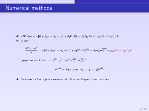
Numerical methods
NGF: ∂tΦ = −[H + β0ρ− pfz + qf2z + β1F · f]Φ− β2A00AΦ + µΦ(t)Φ + λΦ(t)fzΦ
GFDN:
Φ(1) − Φn
τ= −[H + β0ρ
n − pfz + qf2z + β1F
n · f]Φ(1) − β2An00AΦ(1) + µΦn Φn + λΦn fzΦn
,
projection step for Φ(1) = (φ(1)2 , φ
(1)1 , φ
(1)0 , φ
(1)−1, φ
(1)−2)T
Φn+1 = diag(α2, α1, α0, α−1, α−2)Φ(1)
Determine the five projection constants with Mass and Magnetization constraints
32 / 36
Bose-Einstein condensate Spinor Bose-Einstein condensates Spin-1 BEC Spin-2 BEC
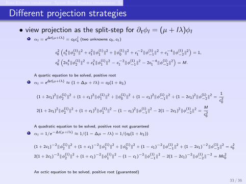
Different projection strategies
• view projection as the split-step for ∂tφl = (µ+ lλ)φlαl = e∆t(µ+lλ) = c0c
l1 (two unknowns c0, c1)
c20
(c4
1‖φ(1)2 ‖
2 + c21‖φ
(1)1 ‖
2 + ‖φ(1)0 ‖
2 + c−21 ‖φ
(1)−1‖
2 + c−41 ‖φ
(1)−2‖
2)
= 1,
c20
(2c4
1‖φ(1)2 ‖
2 + c21‖φ
(1)1 ‖
2 − c−21 ‖φ
(1)−1‖
2 − 2c−41 ‖φ
(1)−2‖
2)
= M.
A quartic equation to be solved, positive root
αl = e∆t(µ+lλ) ≈ (1 + ∆µ + lλ) = c0(1 + lc1)
(1 + 2c1)2‖φ(1)2 ‖
2 + (1 + c1)2‖φ(1)1 ‖
2 + ‖φ(1)0 ‖
2 + (1− c1)2‖φ(1)−1‖
2 + (1− 2c1)2‖φ(1)−2‖
2 =1
c20
2(1 + 2c1)2‖φ(1)2 ‖
2 + (1 + c1)2‖φ(1)1 ‖
2 − (1− c1)2‖φ(1)−1‖
2 − 2(1− 2c1)2‖φ(1)−2‖
2 =M
c20
A quadratic equation to be solved, positive root not guaranteed
αl = 1/e−∆t(µ+lλ) ≈ 1/(1− ∆µ− lλ) = 1/(c0(1 + lc1))
(1 + 2c1)−2‖φ(1)2 ‖
2 + (1 + c1)−2‖φ(1)1 ‖
2 + ‖φ(1)0 ‖
2 + (1− c1)−2‖φ(1)−1‖
2 + (1− 2c1)−2‖φ(1)−2‖
2 = c20
2(1 + 2c1)−2‖φ(1)2 ‖
2 + (1 + c1)−2‖φ(1)1 ‖
2 − (1− c1)−2‖φ(1)−1‖
2 − 2(1− 2c1)−2‖φ(1)−2‖−2 = Mc2
0
An octic equation to be solved, positive root (guaranteed)
33 / 36

Bose-Einstein condensate Spinor Bose-Einstein condensates Spin-1 BEC Spin-2 BEC
Numerical example
54 CONTENTS
Remark 5.1. The idea of determining the projection constants through (5.23)-(5.24) canbe generalized to other spin-F system very easily [47].
-8 0 8x
0
0.15
0.3
M=0φg
0
φg
2
φg
−2
φg
1
φg
−1
-8 0 8x
0
0.15
0.3
M=0.5
-8 0 8x
0
0.15
0.3
M=0
φg
0
φg
2
φg
−2
φg
1
φg
−1
-8 0 8x
0
0.15
0.3
M=0.5
-8 0 8x
0
0.15
0.3
M=0
φg
0
φg
2
φg
−2
φg
1
φg
−1
-8 0 8x
0
0.15
0.3
M=0.5
Figure 5.1: Ground states of spin-2 BEC in Example 5.1 for different magnetization M=0(left column) and M= 0.5 (right column). The set of parameters are those in case (i) forthe top panel, case (iii) for the bottom panel and case (ii) for the middle panel.
Example 5.1. To show the ground state of a spin-2 BEC, we take d= 1, p= q= 0 andV(x)= 1
2 x2 in (5.7) and consider three types of interactions, i.e. (i) β0 =100, β1 =−1 andβ2=2 (ferromagnetic interaction); (ii) β0=100, β1=1 and β2=−2 (nematic interaction); (i-ii) β0=100, β1=10 and β2=2 (cyclic interaction). Figure 5.1 depicts the numerical groundstate profiles under different types of interactions, which shows very rich structures. Inparticular, we find that the single mode approximation in Theorem 5.2 and the vanishingcomponents approximation in Theorem 5.3 hold for the ferromagnetic interactions andthe nematic interactions, respectively.
34 / 36
Bose-Einstein condensate Spinor Bose-Einstein condensates Spin-1 BEC Spin-2 BEC
Summary
Ground states of spin-1/2, 1, 2 BECs
Rigorous ground state properties
Projection methods for computing ground states
35 / 36

Bose-Einstein condensate Spinor Bose-Einstein condensates Spin-1 BEC Spin-2 BEC
THANK YOU!
36 / 36