ground water pollution potential of … water pollution potential of miami county, ohio by paul n....

GROUND WATER POLLUTION POTENTIALOF MIAMI COUNTY, OHIO

BY

PAUL N. SPAHR

GROUND WATER POLLUTION POTENTIAL REPORT NO. 27

OHIO DEPARTMENT OF NATURAL RESOURCES

DIVISION OF WATER

WATER RESOURCES SECTION

OCTOBER, 1995

ii

ABSTRACT

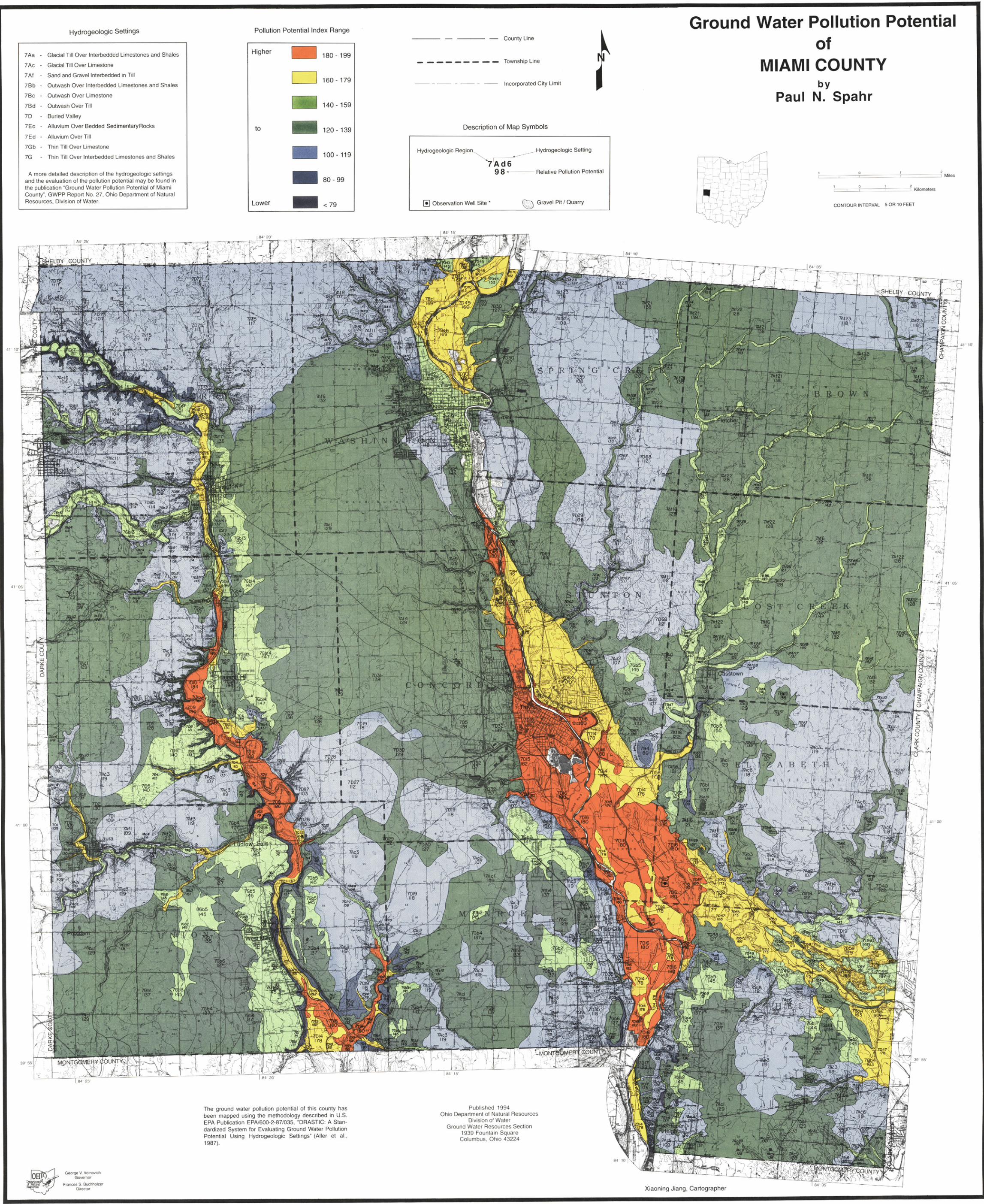
A ground water pollution potential map of Miami County has been prepared using theDRASTIC mapping process. The DRASTIC system consists of two major elements: thedesignation of mappable units, termed hydrogeologic settings, and the superposition of arelative rating system for pollution potential.

Hydrogeologic settings form the basis of the system and incorporate the majorhydrogeologic factors that affect and control ground water movement and occurrenceincluding depth to water, net recharge, aquifer media, soil media, topography, impact of thevadose zone media, and hydraulic conductivity of the aquifer. These factors, which form theacronym DRASTIC, are incorporated into a relative ranking scheme that uses a combinationof weights and ratings to produce a numerical value called the ground water pollutionpotential index. Hydrogeologic settings are combined with the pollution potential indexes tocreate units that can be graphically displayed on a map.

Miami County lies within the Glaciated Central hydrogeologic region. The county iscovered by variable thicknesses of glacial till, lacustrine deposits, and outwash. Theseunconsolidated glacial deposits are underlain by limestone, shale, and shaley limestonebedrock. Ground water yields are dependent on the type of aquifer and vary greatlythroughout the county. Pollution potential indexes are relatively low to moderate in areas oftill or lacustrine cover over bedrock. Buried valleys containing sand and gravel aquifers, andareas covered by outwash have moderate to high vulnerabilities to contamination.

Ground water pollution potential analysis in Miami County resulted in a map with symbolsand colors which illustrate areas of varying ground water contamination vulnerability. Elevenhydrogeologic settings were identified in Miami County with computed ground waterpollution potential indexes ranging from 75 to 190.

The ground water pollution potential analysis program optimizes the use of existing datato rank areas with respect to relative vulnerability to contamination. The ground waterpollution potential map of Miami County has been prepared to assist planners, managers, andlocal officials in evaluating the potential for contamination from various sources of pollution.This information can be used to help direct resources and land use activities to appropriateareas, or to assist in protection, monitoring, and clean-up efforts.

iii

TABLE OF CONTENTS

Number Page

Abstract...........................................................................................................................iiTable of Contents..........................................................................................................iiiList of Figures ................................................................................................................ivList of Tables ..................................................................................................................vAcknowledgements......................................................................................................viIntroduction ...................................................................................................................1Applications of Pollution Potential Maps...................................................................2Summary of the DRASTIC Mapping Process...........................................................3

Hydrogeologic Settings and Factors..............................................................3Weighting and Rating System.........................................................................6Pesticide DRASTIC............................................................................................7Integration of Hydrogeologic Settings and DRASTIC Factors..................11

Interpretation and Use of a Ground Water Pollution Potential Map....................13General Information About MiamiCounty...............................................................14

Physiography.....................................................................................................15Modern Drainage..............................................................................................14Ancestral Drainage and Bedrock Topography.............................................18Glacial Geology..................................................................................................20Bedrock Geology...............................................................................................21Hydrogeology...................................................................................................23Related Studies...................................................................................................24

References ......................................................................................................................25Unpublished Data..........................................................................................................29Appendix A Description of the Logic in Factor Selection........................................30Appendix B Description of the Hydrogeologic Settings and Charts.....................37Erratas.............................................................................................................................53

iv

LIST OF FIGURES

Number Page

1. Format and description of the hydrogeologic setting7Af Sand and Gravel Interbedded in Glacial Till...............................5

2. Description of the hydrogeologic setting7Af1 Sand and Gravel Interbedded in Glacial Till.............................12

3. Location of Miami County...............................................................................154. Generalized Modern Drainage Map...............................................................175. Teays and Deep Stage Drainage in Western Ohio .......................................19

v

LIST OF TABLES

Number Page

1. Assigned weights for DRASTIC features ......................................................72. Ranges and ratings for depth to water..........................................................83. Ranges and ratings for net recharge..............................................................84. Ranges and ratings for aquifer media............................................................95. Ranges and ratings for soil media ..................................................................96. Ranges and ratings for topography...............................................................107. Ranges and ratings for impact of the vadose zone media..........................108. Ranges and ratings for hydraulic conductivity.............................................119. Monthly 30 Year Average for Precipitation and Temperature..................1610. Bedrock Stratigraphy of Miami County, Ohio .............................................2211. Miami County Soils...........................................................................................3412. Hydrogeologic Settings Mapped in Miami County, Ohio..........................37

vi

ACKNOWLEDGEMENTS

The preparation of the Miami County Ground Water Pollution Potential report and mapinvolved the contribution and work of a number of individuals in the Division of Water.Grateful acknowledgement is given to the following individuals for their technical review andmap production, text authorship, report editing, and preparation:

Map preparation and review: Paul SpahrMike AngleMichael Hallfrisch

Map print production and review: Xiaoning JiangMichael HallfrischDavid Orr

Report production and review: Paul SpahrMichael HallfrischMike Angle

Report editing: Rebecca PettyMichael HallfrischPaul SpahrJ. Mc Call-Neubauer

Desktop publishing and report design: David OrrDenise L. Spencer

INTRODUCTION

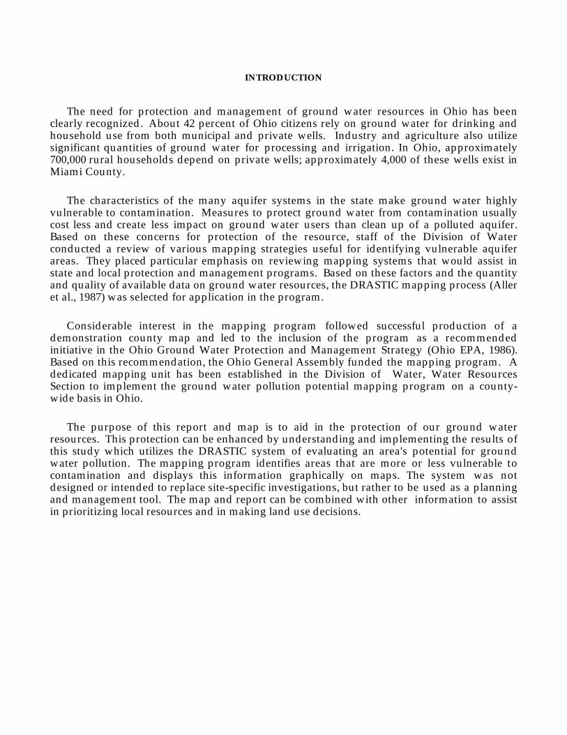
The need for protection and management of ground water resources in Ohio has beenclearly recognized. About 42 percent of Ohio citizens rely on ground water for drinking andhousehold use from both municipal and private wells. Industry and agriculture also utilizesignificant quantities of ground water for processing and irrigation. In Ohio, approximately700,000 rural households depend on private wells; approximately 4,000 of these wells exist inMiami County.

The characteristics of the many aquifer systems in the state make ground water highlyvulnerable to contamination. Measures to protect ground water from contamination usuallycost less and create less impact on ground water users than clean up of a polluted aquifer.Based on these concerns for protection of the resource, staff of the Division of Waterconducted a review of various mapping strategies useful for identifying vulnerable aquiferareas. They placed particular emphasis on reviewing mapping systems that would assist instate and local protection and management programs. Based on these factors and the quantityand quality of available data on ground water resources, the DRASTIC mapping process (Alleret al., 1987) was selected for application in the program.

Considerable interest in the mapping program followed successful production of ademonstration county map and led to the inclusion of the program as a recommendedinitiative in the Ohio Ground Water Protection and Management Strategy (Ohio EPA, 1986).Based on this recommendation, the Ohio General Assembly funded the mapping program. Adedicated mapping unit has been established in the Division of Water, Water ResourcesSection to implement the ground water pollution potential mapping program on a county-wide basis in Ohio.

The purpose of this report and map is to aid in the protection of our ground waterresources. This protection can be enhanced by understanding and implementing the results ofthis study which utilizes the DRASTIC system of evaluating an area's potential for groundwater pollution. The mapping program identifies areas that are more or less vulnerable tocontamination and displays this information graphically on maps. The system was notdesigned or intended to replace site-specific investigations, but rather to be used as a planningand management tool. The map and report can be combined with other information to assistin prioritizing local resources and in making land use decisions.

2

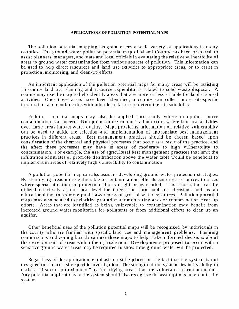
APPLICATIONS OF POLLUTION POTENTIAL MAPS

The pollution potential mapping program offers a wide variety of applications in manycounties. The ground water pollution potential map of Miami County has been prepared toassist planners, managers, and state and local officials in evaluating the relative vulnerability ofareas to ground water contamination from various sources of pollution. This information canbe used to help direct resources and land use activities to appropriate areas, or to assist inprotection, monitoring, and clean-up efforts.

An important application of the pollution potential maps for many areas will be assisting in county land use planning and resource expenditures related to solid waste disposal. Acounty may use the map to help identify areas that are more or less suitable for land disposalactivities. Once these areas have been identified, a county can collect more site-specificinformation and combine this with other local factors to determine site suitability.

Pollution potential maps may also be applied successfully where non-point sourcecontamination is a concern. Non-point source contamination occurs where land use activitiesover large areas impact water quality. Maps providing information on relative vulnerabilitycan be used to guide the selection and implementation of appropriate best managementpractices in different areas. Best management practices should be chosen based uponconsideration of the chemical and physical processes that occur as a resut of the practice, andthe affect these processes may have in areas of moderate to high vulnerability tocontamination. For example, the use of agricultural best management practices that limit theinfiltration of nitrates or promote denitrification above the water table would be beneficial toimplement in areas of relatively high vulnerability to contamination.

A pollution potential map can also assist in developing ground water protection strategies.By identifying areas more vulnerable to contamination, officials can direct resources to areaswhere special attention or protection efforts might be warranted. This information can beutilized effectively at the local level for integration into land use decisions and as aneducational tool to promote public awareness of ground water resources. Pollution potentialmaps may also be used to prioritize ground water monitoring and/or contamination clean-upefforts. Areas that are identified as being vulnerable to contamination may benefit fromincreased ground water monitoring for pollutants or from additional efforts to clean up anaquifer.

Other beneficial uses of the pollution potential maps will be recognized by individuals inthe county who are familiar with specific land use and management problems. Planningcommissions and zoning boards can use these maps to help make informed decisions aboutthe development of areas within their jurisdiction. Developments proposed to occur withinsensitive ground water areas may be required to show how ground water will be protected.

Regardless of the application, emphasis must be placed on the fact that the system is notdesigned to replace a site-specific investigation. The strength of the system lies in its ability tomake a "first-cut approximation" by identifying areas that are vulnerable to contamination.Any potential applications of the system should also recognize the assumptions inherent in thesystem.

3

SUMMARY OF THE DRASTIC MAPPING PROCESS

The system chosen for implementation of a ground water pollution potential mappingprogram in Ohio, DRASTIC, was developed by the National Water Well Association for theUnited States Environmental Protection Agency. A detailed discussion of this system can befound in Aller et al., (1987).

The DRASTIC mapping system allows the pollution potential of any area to be evaluatedsystematically using existing information. The vulnerability to contamination is a combinationof hydrogeologic factors, anthropogenic influences, and sources of contamination in any givenarea. The DRASTIC system focuses only on those hydrogeologic factors which influenceground water pollution potential. The system consists of two major elements: the designationof mappable units, termed hydrogeologic settings, and the superposition of a relative ratingsystem to determine pollution potential.

The application of DRASTIC to an area requires the recognition of a set of assumptionsmade in the development of the system. DRASTIC evaluates the pollution potential of anarea, assuming a contaminant with the mobility of water introduced at the surface and flushedinto the ground water by precipitation. Most important, DRASTIC cannot be applied to areassmaller than 100 acres in size and is not intended or designed to replace site-specificinvestigations.

Hydrogeologic Settings and Factors

To facilitate the designation of mappable units, the DRASTIC system used the frameworkof an existing classification system developed by Heath (1984), which divides the United Statesinto 15 ground water regions based on the factors in a ground water system that affectoccurrence and availability.

Within each major hydrogeologic region, smaller units representing specific hydrogeologicsettings are identified. Hydrogeologic settings form the basis of the system and represent acomposite description of the major geologic and hydrogeologic factors that control groundwater movement into, through, and out of an area. A hydrogeologic setting represents amappable unit with common hydrogeologic characteristics and, as a consequence, commonvulnerability to contamination (Aller et al., 1987).

4

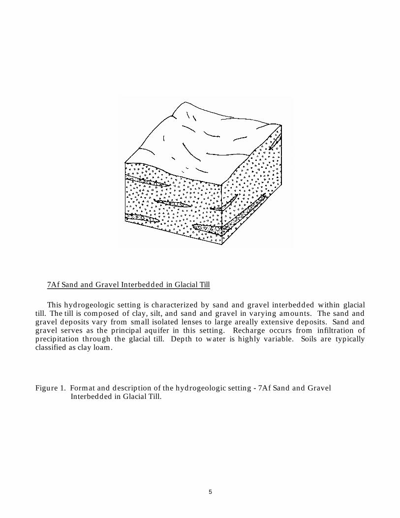
Figure 1 illustrates the format and description of a typical hydrogeologic setting foundwithin Miami County. Inherent within each hydrogeologic setting are the physicalcharacteristics which affect the ground water pollution potential. These characteristics orfactors identified during the development of the DRASTIC system include:

D - Depth to WaterR - Net RechargeA - Aquifer MediaS - Soil MediaT - TopographyI - Impact of the Vadose Zone MediaC - Conductivity (Hydraulic) of the Aquifer

These factors incorporate concepts and mechanisms such as attenuation, retardation andtime or distance of travel of a contaminant with respect to the physical characteristics of thehydrogeologic setting. Broad consideration of these factors and mechanisms coupled withexisting conditions in a setting provide a basis for determination of the area's relativevulnerability to contamination.

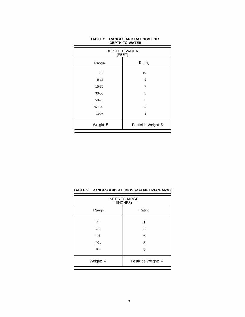
Depth to water is considered to be the depth from the ground surface to the water table inunconfined aquifer conditions or the depth to the top of the aquifer under confined aquiferconditions. The depth to water determines the distance a contaminant would have to travelbefore reaching the aquifer. The greater the distance the contaminant has to travel, thegreater the opportunity for attenuation to occur or restriction of movement by relativelyimpermeable layers.

Net recharge is the total amount of water reaching the land surface that infiltrates into theaquifer measured in inches per year. Recharge water is available to transport a contaminantfrom the surface into the aquifer and also affects the quantity of water available for dilutionand dispersion of a contaminant. Factors to be included in the determination of net rechargeinclude contributions due to infiltration of precipitation, in addition to infiltration from rivers,streams and lakes, irrigation, and artificial recharge.

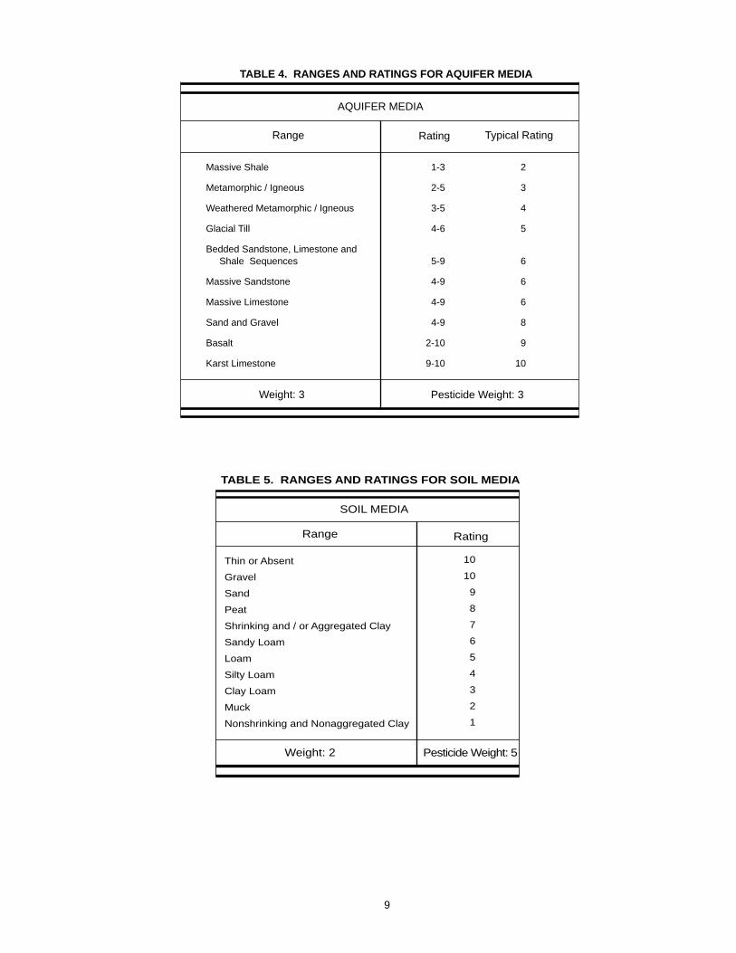
Aquifer media represents consolidated or unconsolidated rock material capable of yieldingsufficient quantities of water for use. Aquifer media accounts for the various physicalcharacteristics of the rock that provide mechanisms of attenuation, retardation, and flowpathways that affect a contaminant reaching and moving through an aquifer.

5

7Af Sand and Gravel Interbedded in Glacial Till

This hydrogeologic setting is characterized by sand and gravel interbedded within glacialtill. The till is composed of clay, silt, and sand and gravel in varying amounts. The sand andgravel deposits vary from small isolated lenses to large areally extensive deposits. Sand andgravel serves as the principal aquifer in this setting. Recharge occurs from infiltration ofprecipitation through the glacial till. Depth to water is highly variable. Soils are typicallyclassified as clay loam.

Figure 1. Format and description of the hydrogeologic setting - 7Af Sand and GravelInterbedded in Glacial Till.

6

Soil media refers to the upper six feet of the unsaturated zone that is characterized bysignificant biological activity. The type of soil media can influence the amount of recharge thatcan move through the soil column due to variations in soil permeability. Various soil typesalso have the ability to attenuate or retard a contaminant as it moves throughout the soilprofile. Soil media is based on textural classifications of soils and considers relative thicknessesand attenuation characteristics of each profile within the soil.

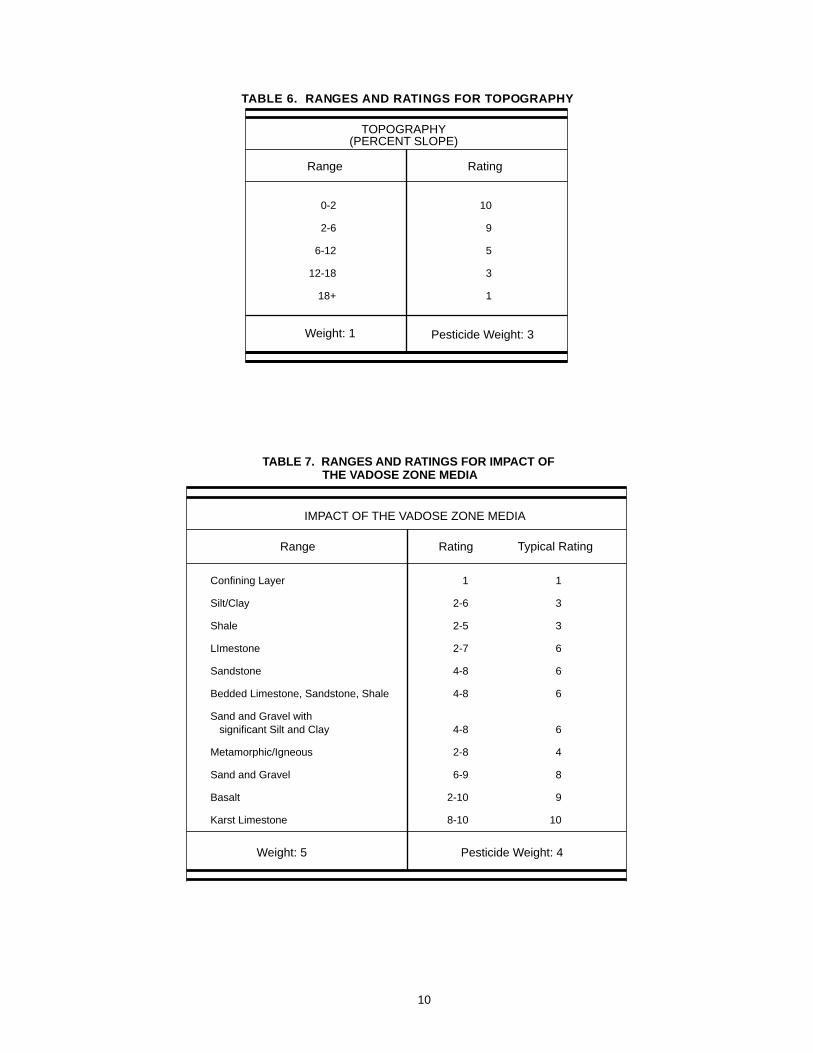
Topography refers to the slope of the land expressed as percent slope. The amount ofslope in an area affects the likelihood that a contaminant will run off from an area or beponded and ultimately infiltrate into the subsurface. Topography also affects soildevelopment and often can be used to help determine the direction and gradient of groundwater flow under water table conditions.

The impact of the vadose zone media refers to the attenuation and retardation processesthat can occur as a contaminant moves through the unsaturated zone above the aquifer. Thevadose zone represents that area below the soil horizon and above the aquifer that isunsaturated or discontinuously saturated. Various attenuation, travel time, and distancemechanisms related to the types of geologic materials present can affect the movement ofcontaminants in the vadose zone. Where an aquifer is unconfined, the vadose zone mediarepresents the materials below the soil horizon and above the water table. Under confinedaquifer conditions, the vadose zone is simply referred to as a confining layer. The presence ofthe confining layer in the unsaturated zone significantly impacts the pollution potential of theground water in an area.

Hydraulic conductivity of an aquifer is a measure of the ability of the aquifer to transmitwater, and is also related to ground water velocity and gradient. Hydraulic conductivity isdependent upon the amount and interconnectivity of void spaces and fractures within aconsolidated or unconsolidated rock unit. Higher hydraulic conductivity typically correspondsto higher vulnerability to contamination. Hydraulic conductivity considers the capability for acontaminant that reaches an aquifer to be transported throughout that aquifer over time.

Weighting and Rating System

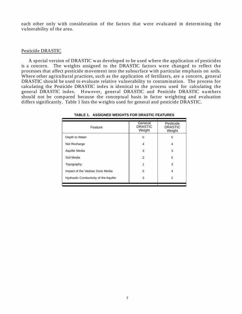
DRASTIC uses a numerical weighting and rating system that is combined with theDRASTIC factors to calculate a ground water pollution potential index or relative measure ofvulnerability to contamination. The DRASTIC factors are weighted from 1 to 5 according totheir relative importance to each other with regard to contamination potential (Table 1). Eachfactor is then divided into ranges or media types and assigned a rating from 1 to 10 based ontheir significance to pollution potential (Tables 2-8). The rating for each factor is selected basedon available information and professional judgement. The selected rating for each factor ismultiplied by the assigned weight for each factor. These numbers are summed to calculate theDRASTIC or pollution potential index.

Once a DRASTIC index has been calculated, it is possible to identify areas that are morelikely to be susceptible to ground water contamination relative to other areas. The higher theDRASTIC index, the greater the vulnerability to contamination. The index generated providesonly a relative evaluation tool and is not designed to produce absolute answers or to representunits of vulnerability. Pollution potential indexes of various settings should be compared to

7

each other only with consideration of the factors that were evaluated in determining thevulnerability of the area.

Pesticide DRASTIC

A special version of DRASTIC was developed to be used where the application of pesticidesis a concern. The weights assigned to the DRASTIC factors were changed to reflect theprocesses that affect pesticide movement into the subsurface with particular emphasis on soils.Where other agricultural practices, such as the application of fertilizers, are a concern, generalDRASTIC should be used to evaluate relative vulnerability to contamination. The process forcalculating the Pesticide DRASTIC index is identical to the process used for calculating thegeneral DRASTIC index. However, general DRASTIC and Pesticide DRASTIC numbersshould not be compared because the conceptual basis in factor weighting and evaluationdiffers significantly. Table 1 lists the weights used for general and pesticide DRASTIC.

FeatureGeneral

DRASTICWeight

TABLE 1. ASSIGNED WEIGHTS FOR DRASTIC FEATURES

Depth to Water

Net Recharge

Aquifer Media

Soil Media

Topography

Impact of the Vadose Zone Media

Hydraulic Conductivity of the Aquifer

5

4

3

2

1

5

3

PesticideDRASTIC

Weight

5

4

3

5

3

4

2

8

10

9

7

5

3

2

1

0-5

5-15

15-30

30-50

50-75

75-100

100+

Weight: 5 Pesticide Weight: 5

Range Rating

DEPTH TO WATER(FEET)

TABLE 2. RANGES AND RATINGS FOR DEPTH TO WATER

TABLE 3. RANGES AND RATINGS FOR NET RECHARGE

NET RECHARGE(INCHES)

Range Rating


0-2

2-4

4-7

7-10

10+

1

3

6

8

9

9


Range Rating Typical Rating

AQUIFER MEDIA

TABLE 4. RANGES AND RATINGS FOR AQUIFER MEDIA

Massive Shale

Metamorphic / Igneous

Weathered Metamorphic / Igneous

Glacial Till

Bedded Sandstone, Limestone and Shale Sequences

Massive Sandstone

Massive Limestone

Sand and Gravel

Basalt

Karst Limestone

1-3

2-5

3-5

4-6

5-9

4-9

4-9

4-9

2-10

9-10

2

3

4

5

6

6

6

8

9

10

Pesticide Weight: 5Weight: 2

SOIL MEDIA

Thin or Absent

Gravel

Sand

Peat

Shrinking and / or Aggregated Clay

Sandy Loam

Loam

Silty Loam

Clay Loam

Muck

Nonshrinking and Nonaggregated Clay

10

10

9

8

7

6

5

4

3

2

1

TABLE 5. RANGES AND RATINGS FOR SOIL MEDIA

Range Rating

10

TABLE 6. RANGES AND RATINGS FOR TOPOGRAPHY

TOPOGRAPHY(PERCENT SLOPE)

Range Rating


0-2

2-6

6-12

12-18

18+

10

9

5

3

1


Range Rating Typical Rating

IMPACT OF THE VADOSE ZONE MEDIA

TABLE 7. RANGES AND RATINGS FOR IMPACT OF THE VADOSE ZONE MEDIA

Confining Layer

Silt/Clay

Shale

LImestone

Sandstone

Bedded Limestone, Sandstone, Shale

Sand and Gravel with significant Silt and Clay

Metamorphic/Igneous

Sand and Gravel

Basalt

Karst Limestone

1

2-6

2-5

2-7

4-8

4-8

4-8

2-8

6-9

2-10

8-10

1

3

3

6

6

6

6

4

8

9

10

11


Range Rating

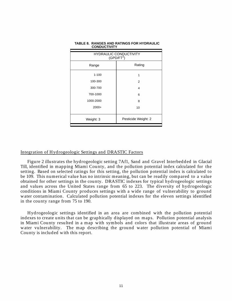
TABLE 8. RANGES AND RATINGS FOR HYDRAULIC CONDUCTIVITY

HYDRAULIC CONDUCTIVITY(GPD/FT2)

1-100

100-300

300-700

700-1000

1000-2000

2000+

1

2

4

6

8

10

Integration of Hydrogeologic Settings and DRASTIC Factors

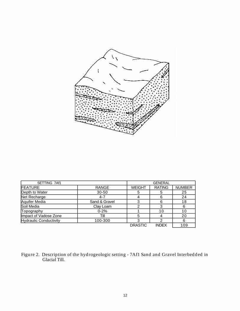
Figure 2 illustrates the hydrogeologic setting 7Af1, Sand and Gravel Interbedded in GlacialTill, identified in mapping Miami County, and the pollution potential index calculated for thesetting. Based on selected ratings for this setting, the pollution potential index is calculated tobe 109. This numerical value has no intrinsic meaning, but can be readily compared to a valueobtained for other settings in the county. DRASTIC indexes for typical hydrogeologic settingsand values across the United States range from 65 to 223. The diversity of hydrogeologicconditions in Miami County produces settings with a wide range of vulnerability to groundwater contamination. Calculated pollution potential indexes for the eleven settings identifiedin the county range from 75 to 190.

Hydrogeologic settings identified in an area are combined with the pollution potentialindexes to create units that can be graphically displayed on maps. Pollution potential analysisin Miami County resulted in a map with symbols and colors that illustrate areas of groundwater vulnerability. The map describing the ground water pollution potential of MiamiCounty is included with this report.

12

SETTING 7Af1 GENERALFEATURE RANGE WEIGHT RATING NUMBERDepth to Water 30-50 5 5 25Net Recharge 4-7 4 6 24Aquifer Media Sand & Gravel 3 6 18Soil Media Clay Loam 2 3 6Topography 0-2% 1 10 10Impact of Vadose Zone Till 5 4 20Hydraulic Conductivity 100-300 3 2 6

DRASTIC INDEX 109

Figure 2. Description of the hydrogeologic setting - 7Af1 Sand and Gravel Interbedded inGlacial Till.

13

INTERPRETATION AND USE OF A GROUND WATER POLLUTION POTENTIAL MAP

The application of the DRASTIC system to evaluate an area's vulnerability tocontamination produces hydrogeologic settings with corresponding pollution potentialindexes. The higher the pollution potential index, the greater the susceptibility tocontamination. This numeric value determined for one area can be compared to the pollutionpotential index calculated for another area.

The map accompanying this report displays both the hydrogeologic settings identified inthe county and the associated pollution potential indexes calculated in those hydrogeologicsettings. The symbols on the map represent the following information:

7Af1 - defines the hydrogeologic region and setting109 - defines the relative pollution potential

Here the first number (7) refers to the major hydrogeologic region and the upper andlower case letters (Af) refer to a specific hydrogeologic setting. The following number (1)references a certain set of DRASTIC parameters that are unique to this setting and aredescribed in the corresponding setting chart. The second number (109) is the calculatedpollution potential index for this unique setting. The charts for each setting provide areference to show how the pollution potential index was derived in an area.

The maps are color-coded using ranges depicted on the map legend. The color codes usedare part of a national color-coding scheme developed to assist the user in gaining a generalinsight into the vulnerability of the ground water in the area. The color codes were chosen torepresent the colors of the spectrum, with warm colors (red, orange, and yellow),representing areas of higher vulnerability (higher pollution potential indexes), and cool colors(greens, blues, and violet), representing areas of lower vulnerability to contamination.

The map also includes information on the location of a selected observation well. Availableinformation on this observation well is referenced in Appendix A, Description of the Logic inFactor Selection. Large man-made features such as landfills, quarries, or strip mines have alsobeen marked on the map for reference.

14

GENERAL INFORMATION ABOUT MIAMI COUNTY

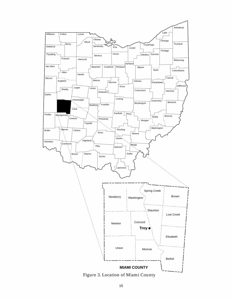
Miami County occupies approximately 407 square miles in west-central Ohio. The countyis divided into 12 townships and is bordered on the west by Darke County, on the north byShelby County, on the east by Clark County, and on the south by Montgomery County(Figure 3). The county seat is the city of Troy. The population of Miami County wasestimated to be 93,152 in 1990 (U.S. Department of Commerce, 1990).

Physiography

Miami County lies within the Till Plains section of the Central Lowlands physiographicprovince (Fenneman, 1938). The topography of the county is characterized by level to gentlyrolling terrain dissected by modern drainages. The surficial features of the county arepredominantly glacial in origin with the exception of bedrock outcrops throughout the county.The maximum relief in the county is approximately 390 feet.

Climate

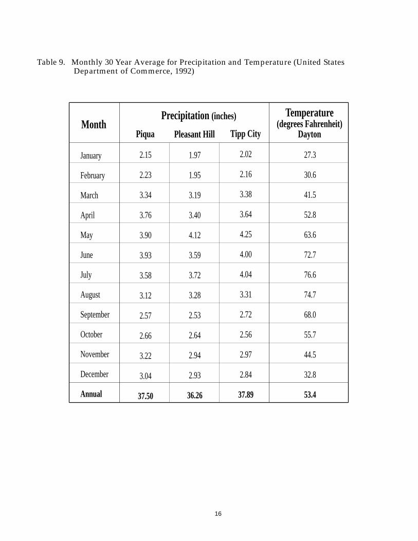
The thirty-year (1961-1990) annual average temperature for the region including MiamiCounty, as recorded in Dayton Ohio, is 53.4 degrees Fahrenheit (U.S. Department ofCommerce, 1992). January, the coldest month, has a thirty-year monthly average of 27.3degrees Fahrenheit. July is the warmest month with a thirty-year monthly average of 76.6degrees Fahrenheit (Table 9).

The precipitation for Miami County has been recorded at stations in Piqua, Pleasant Hill,and Tipp City. The thirty-year (1961-1990) average annual precipitation for these locations are37.50 inches, 36.26 inches, and 37.89 inches, respectively (U.S. Department of Commerce, 1992).The wettest month is typically May and the driest month is January (Table 9).

Modern Drainage

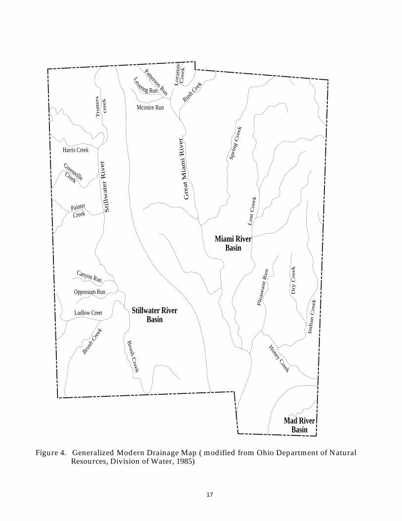
Miami County lies within the Great Miami River Basin (Ohio Department of NaturalResources, 1985). Major sub-basins of the Great Miami River Basin in Miami County includethe Stillwater River Basin (Walker, 1960a), the Miami River Basin (Middle Portion) (Walker,1960b, c), and the Lower Mad River Basin (Walker, 1960c). Figure 4 is a generalized map ofMiami County showing the modern drainage system and accompanying basins.

15

Lake

Geauga

Williams Fulton Lucas

OttawaWood

HenryDefiance

Paulding

Putnam Hancock

Sandusky Erie

HuronSeneca

Wyandot Crawford Richland

Ashland

Lorain

Cuyahoga

Ashtabula

Trumbull

Portage

SummitMedina

WayneStark Columbiana

Mahoning

Carroll

Holmes

Van Wert

AllenHardin

MarionMorrow

Knox

Coshocton

Jefferson

Harrison

Tuscarawas

MercerAuglaize

Shelby

Darke

MiamiChampaign

Logan Union

Delaware

Licking

FranklinMadison

Clark

MuskingumGuernsey

Belmont

MonroeNoble

Fairfield Perry

Morgan

Washington

Athens

Meigs

Hocking

Pickaway

Fayette

Greene

MontgomeryPreble

Butler Warren ClintonRoss

Highland

Pike

HamiltonClermont

Brown AdamsScioto

Jackson

Vinton

Gallia

Lawrence

MIAMI COUNTY

Troy

Newberry Washington

Spring Creek

Brown

Newton Concord

Staunton

Lost Creek

Union Monroe

Bethel

Elisabeth

Figure 3. Location of Miami County

16

Table 9. Monthly 30 Year Average for Precipitation and Temperature (United StatesDepartment of Commerce, 1992)

MonthPrecipitation (inches) Temperature

(degrees Fahrenheit)DaytonPiqua Pleasant Hill Tipp City

January

February

March

April

May

June

July

August

September

October

November

December

Annual

2.15

2.23

3.34

3.76

3.90

3.93

3.58

3.12

2.57

2.66

3.22

3.04

37.50

1.97

1.95

3.19

3.40

4.12

3.59

3.72

3.28

2.53

2.64

2.94

2.93

36.26

2.02

2.16

3.38

3.64

4.25

4.00

4.04

3.31

2.72

2.56

2.97

2.84

37.89

27.3

30.6

41.5

52.8

63.6

72.7

76.6

74.7

68.0

55.7

44.5

32.8

53.4

17

Stillwater River Basin

Miami River Basin

Mad River Basin

Tro

tters

cre

ek

Harris Creek

Greenville Creek

Painter

Creek

Canyon Run

Oppossum Run

Ludlow Creet

Brush

Creek

Bru

sh C

reek

Patterson Run

Mcintire Run

Levering Run

Rush C

eek

Gre

at

Mia

mi

Riv

er

Sti

llw

ate

r R

iver S

pri

ng C

reek

Lost

Cre

ek

Honey Creek

Ple

asea

nt

Run

Dry

Cre

ek

India

n C

reek

Lora

mie

C

reek

Figure 4. Generalized Modern Drainage Map ( modified from Ohio Department of NaturalResources, Division of Water, 1985)

18

The Stillwater River Basin in Miami County is drained by the southerly flowing StillwaterRiver and its tributaries. The portion of this basin that lies in Miami County occupiesapproximately the western third of the county. The average daily discharge for a gaugingstation on the Stillwater River at Pleasant Hill from 1917 to 1992 is 447 cubic feet per second(U.S. Geological Survey, 1992). The largest tributary to the Stillwater River is GreenvilleCreek. Average discharge for a 61 year period at a gauging station for Greenville Creek, nearBradford Ohio, is 176 cubic feet per second (U.S. Geological Survey, 1992). Minor tributaries tothe Stillwater River include Trotters Creek, Harris Run, Painter Creek, Canyon Run, OpossumRun, Rocky Run, Brush Creek, and Jones Run (Figure 4).

The Miami River Basin (Middle Portion) is drained by the Great Miami River and itstributaries. The portion of this basin that is present in Miami County occupies theapproximate eastern two thirds of the county. The Great Miami River is the largest river inthe county. Average daily discharge for a gauging station at Troy from 1963 to 1992 is 814cubic feet per second (U.S. Geological Survey, 1992). The largest tributaries to the Great MiamiRiver in Miami County include Spring Creek, Lost Creek, and Honey Creek (Figure 4).

A small portion of the Lower Mad River Basin is present in southeastern Miami County.Surficial drainages that are part of this basin are limited to small ephemeral tributaries to MudCreek (Figure 4).

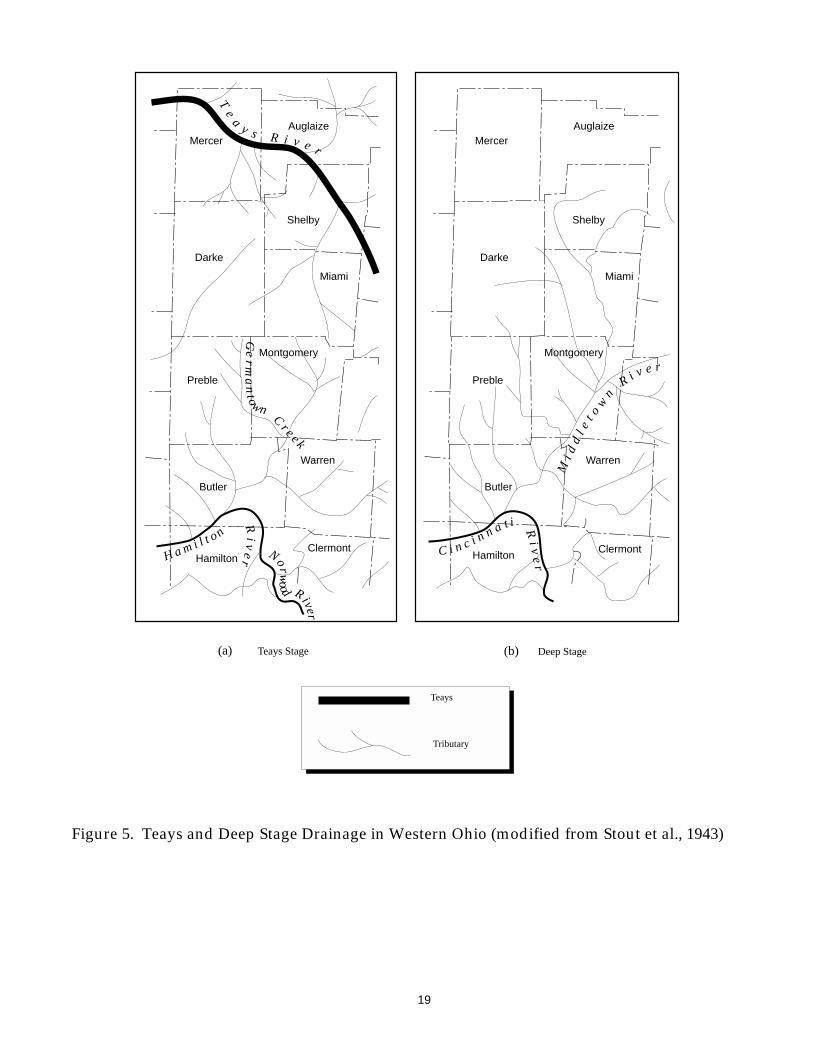
Ancestral Drainage and Bedrock Topography

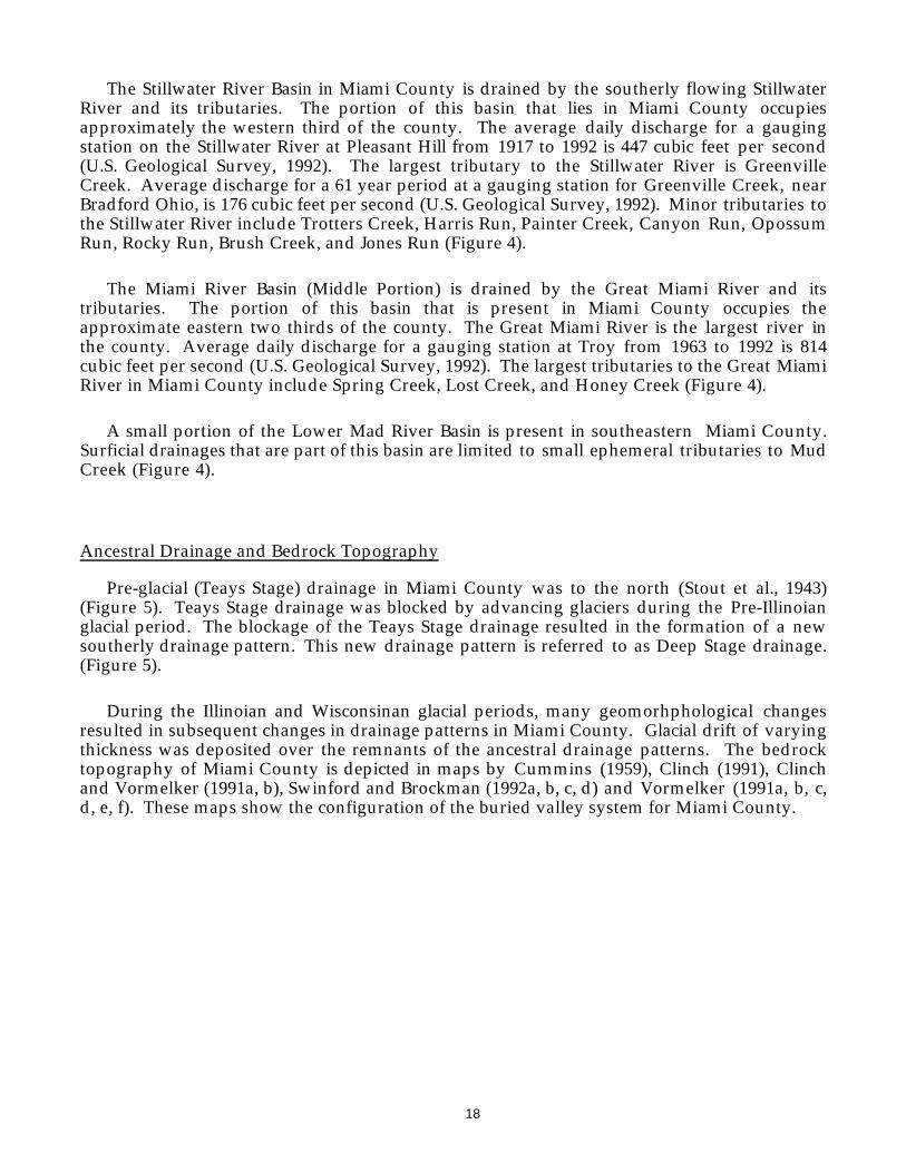
Pre-glacial (Teays Stage) drainage in Miami County was to the north (Stout et al., 1943)(Figure 5). Teays Stage drainage was blocked by advancing glaciers during the Pre-Illinoianglacial period. The blockage of the Teays Stage drainage resulted in the formation of a newsoutherly drainage pattern. This new drainage pattern is referred to as Deep Stage drainage.(Figure 5).

During the Illinoian and Wisconsinan glacial periods, many geomorhphological changesresulted in subsequent changes in drainage patterns in Miami County. Glacial drift of varyingthickness was deposited over the remnants of the ancestral drainage patterns. The bedrocktopography of Miami County is depicted in maps by Cummins (1959), Clinch (1991), Clinchand Vormelker (1991a, b), Swinford and Brockman (1992a, b, c, d) and Vormelker (1991a, b, c,d, e, f). These maps show the configuration of the buried valley system for Miami County.

19

Teays

Tributary

(a) Teays Stage (b) Deep Stage

MercerAuglaize

Darke

Shelby

Miami

Preble

Montgomery

Butler

Warren

HamiltonClermont

Mi d

dl e

t ow

n

R i v e r

MercerAuglaize

Darke

Shelby

Miami

Preble

Montgomery

Butler

Warren

HamiltonClermont C i n c i n n a t i R

i ve

rH a m i l t o n R

ive

rG

er

ma

ntow n C

r e e k

River

Norwood

Te

a

y s R i v e r

Figure 5. Teays and Deep Stage Drainage in Western Ohio (modified from Stout et al., 1943)

20

Glacial Geology

During the Pleistocene Epoch at least four stages of glaciation occurred in North America.Evidence for glaciation during the Wisconsinan, Illinoian, and Pre-Illinoian (Kansan) stagesexist in southwestern Ohio. Surficial glacial drift throughout Miami County was depositedduring the Wisconsinan stage (Goldthwait et al., 1961). Drift was deposited in the form of ice-laid (end moraines, ground moraines) and water-laid deposits (kames, outwash).

Drift deposits range in thickness from 0 to approximately 400 feet in Miami County. Thethickest deposits of drift are typically located beneath end moraines or filling valleys that havebeen buried by glacial deposits. The thickest deposit of drift can be found in the northeasternsection of the county, to the north of the Village of Lena. At this location an end moraineoverlies a buried valley. Drift, composed of sand and gravel lenses interbedded in till, isapproximately 400 feet thick at this site. There are many locations in Miami County wheredrift is absent and bedrock is exposed. Areas in which the till cover is less than 10 feet havebeen mapped as Thin Till over Limestone (7Gb) or as Thin Till over Bedded SedimentaryRocks (7G).

Portions of three end moraines are present in Miami County (Goldthwait et al, 1961; OhioDepartment of Natural Resources, Division of Geological Survey, 1993). End moraines arebelts of hummocky terrain that are generally higher than the adjoining land and arecomposed of till. Till is predominantly unsorted, unconsolidated, and unstratified driftcomposed of a heterogeneous mixture of clay, silt, sand, and coarser rocks. End moraines areclassically described as forming along the margins of a glacier where the ice was stagnant orretreating. The Bloomer and Union City End Moraines are located in the northwestern cornerof Miami County. The Farmersville End Moraine is located on the eastern side of the county.

Associated with the Union City and Farmersville moraines are an anomalously highconcentration of boulders referred to as the Boulder Belt (Goldthwait et al., 1961). Theconcentration of boulders in this area is in the range of 10 to 100 per acre. The majority ofboulders are usually crystalline rocks of Canadian origin. Field observations in 1991 revealeda high concentration of boulders lining fences in Sections 23 and 29 of Elizabeth Township.These were apparently moved to the fence line by farmers in the area during agriculturaloperations.

Most of the surficial glacial deposits of Miami County are in the form of ground moraine.Ground moraine are extensive, broad, flat-surfaced deposits of till. The till was depositeddiscontinuously by ice advancing over bedrock or over older glacial deposits. Groundmoraine covers most of the county. Till thicknesses in ground moraine are typically less thanadjacent end moraines.

Extensive deposits of outwash are present in Miami County. Outwash is well sorted,highly stratified, commonly crossbedded deposits of sand and gravel. The sand and gravelwas deposited by meltwater streams that flowed in front of the glacier. Most of the outwashin Miami County was deposited as outwash fans or as valley trains. Some of the outwash maybe covered by a thin layer of recent alluvium or loess. Lenses of till and silt are commonwithin the outwash deposits. Outwash, of various thicknesses, is found in most of the GreatMiami River Valley with the exception of a narrow part of the river valley between Piqua andFarrington (Norris and Speiker, 1961). Outwash is also present in the vicinity of majorportions of the Stillwater River Valley and in areas adjacent to Honey Creek (OhioDepartment of Natural Resources, Division of Geological Survey, 1993).

21

Kames are high, steep hummocks composed of bedded sand and gravel deposited bywater flowing through channels, tubes, or pits in the melting glacier. Crossbedding, dippingbeds, and channel structures are common (Goldthwait et al, 1961). A high percentage ofkames are found adjacent to Honey Creek in Elizabeth and Bethel Townships (OhioDepartment of Natural Resources, Division of Geological Survey, 1993).

Bedrock Geology

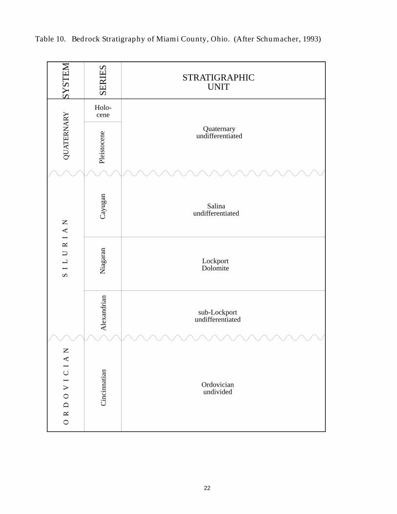
The bedrock of Miami County is composed of upper Ordovician to upper Silurian agesedimentary rocks (Table 10). The bedrock units consist of undifferentiated Ordovician ageinterbedded limestone and shales overlain by Silurian age Sub Lockport, Lockport, andundifferentiated Salina limestones and dolomites. These formations lie on the western flank ofthe Cincinnati Arch and have an approximate dip of five to ten feet per mile to the northwest(Norris and Fidler, 1973). The configuration of the bedrock geology of Miami County can beseen in the Bedrock Geology maps of Schumacher (Schumacher, 1991a, b, c, d, e, f, g, h).

The upper Ordovician in Miami County consists of shale with minor limestone anddolomite. The shale portion is described as gray, calcareous to dolomitic, locally silty, thinly tothickly bedded, and sparsely to abundantly fossiliferous. The limestone portion is gray,micritic, thin to medium irregular wavy to planar bedded, has a rare vuggy to intergranularporosity, and is fossiliferous. The dolomite is gray, finely to coarsely crystalline, has a rarevuggy porosity and rare vertical fractures, and is laminated to medium bedded (Schumacher,1993).

22

Table 10. Bedrock Stratigraphy of Miami County, Ohio. (After Schumacher, 1993)

SYST

EM

SER

IES

STRATIGRAPHICUNIT

QU

AT

ER

NA

RY

Holo-cene

Plei

stoc

ene

S I

L U

R I

A N

O R

D O

V I

C I

A N

Cay

ugan

Nia

gara

nA

lexa

ndri

anC

inci

nnat

ian

Quaternaryundifferentiated

Salinaundifferentiated

LockportDolomite

sub-Lockportundifferentiated

Ordovicianundivided

23

The Lower Silurian in Miami County consist of undiferentiated sub-Lockport dolomite andminor shale, and Lockport dolomite with rare chert and shale. The sub-Lockport dolomite isdescribed as light gray to brown, micro to coarsely crystalline, has open vertical fractures, thinto thick irregular to planar bedding, and is sparsely fossiliferous. The minor shale portion ofthe sub Lockport is described as greenish-gray, dolomitic, with laminated to thin irregular towavy bedding (Schumacher, 1993). The Lockport dolomite is described as white to gray,micro to coarsely crystalline, vuggy, with fractures perpendicular to massive to thick beds, andis commonly fossiliferous (Schumacher, 1993).

The upper Silurian bedrock in Miami County is composed of undifferentiated Salinadolomite and rare shale. The undifferentiated Salina is gray, microcrystaline to fine grained,intergranular to vuggy porosity, with open vertical fractures, laminated to thinly bedded andsparsely fossiliferous (Schumacher, 1993).

There are several locations in Miami County in which the bedrock is exposed or outcropsat the ground surface. Bedrock outcrops are found in the uplands, adjacent to the StillwaterRiver, near West Milton, Ludlow Falls, Pleasant Hill, and Covington. Bedrock outcrops arelocated in the uplands, adjacent to the Great Miami River floodplain, in the vicinity of Piqua,Troy, and Tipp City. Waterfalls on Greenville Creek and Ludlow Creek flow directly over thebedrock which outcrops on the adjacent banks of these creeks. Several limestone quarries inthe county have fresh exposures of bedrock (Weisgarber, 1992). Gregory Stone (UnionTownship), Piqua Mineral Division (Spring Creek Township), and C.F. Poppelman, Inc.(Newberry Township) are located in areas where the bedrock is close to the surface.

Hydrogeology

An aquifer is a saturated permeable geologic unit that can transmit significant quantities ofwater under hydraulic gradients to yield economic amounts of water to wells (Freeze andCherry, 1979). Aquifer media in Miami County can be classified as consolidated (bedrock) andunconsolidated (sand and gravel) formations. Consolidated aquifers in Miami County includethe undifferentiated Ordovician age interbedded limestone and shales, and the Silurian agelimestones and dolomites. Unconsolidated aquifers in the county are composed of sand andgravel deposits of varying extent, thickness and composition. These sand and gravel aquiferswere deposited as "lenses" within till or as outwash filling buried valleys.

The undifferentiated Ordovician interbedded limestone and shale aquifer system istypically found below elevations of 875 feet in Miami County (Schumacher, 1991a, b, c, d, e, f,g, h). The Ordivician aquifer outcrops in some areas in Miami County but is typically found inthe buried valleys where it is covered with varying thicknesses of drift. The Ordovician ageinterbedded limestone and shale is a poor aquifer due to the low permeability of theinterbedded limestone and shale formations. It is usually considered a lower confining unitrelative to more permeable overlying aquifers that are typically present. Well Log andDrilling Reports show that wells are developed in this aquifer only when no significantoverlying aquifer of higher permeability is present. Yields from domestic wells are meagerand usually less than two gallons per minute (gpm) (Schmidt, 1984).

The Silurian limestone and dolomite aquifer system is present throughout the county atelevations usually greater than 875 feet (Schumacher, 1991a, b, c, d, e, f, g, h). The

24

permeability of this aquifer system is variable and is primarily dependent on the amount ofjoints, fractures, and solution openings, and the degree of interconnection between them. Thisaquifer system exhibits unconfined to semi-confined conditions depending on the amount andcomposition of any overlying unconsolidated deposits. Wells developed in this aquifer systemare highly variable and yields range from 5 to 75 gpm (Schmidt, 1984).

The unconsolidated sand and gravel aquifers in Miami County occurring as "lenses"interbedded within till are found throughout the county. Well Log and Drilling Reports showthat these sand and gravel aquifers show a wide range of variability in their vertical andhorizontal extent, degree of sorting, and texture. Norris and Speiker (1961) state, "Locally, thedeposits may consist of clean well-sorted coarse sand and gravel, ideally suited to thedevelopment of wells, but elsewhere they may be clayey, or made up chiefly of fine sand,making well development difficult or impractible". These variations are reflected in the yieldsobtained from the sand and gravel aquifers. Domestic wells developed in sand and gravelinterbedded in till typically yield 3 to 10 gpm (Schmidt, 1984). Well Logs and Drilling Reportsfor this type of aquifer show that occasional yields of up to 50 gpm can be obtained with aproperly constructed well in thicker, well sorted sand and gravel lenses.

Outwash sand and gravel deposits within buried valleys are the highest yielding aquifers inMiami County. Regionally extensive, thick deposits of sand and gravel adjacent to the GreatMiami River are capable of producing in excess of 1000 gpm (Schmidt, 1984). Outwashdeposits overlying buried valleys adjacent to Honey Creek and the Stillwater River arecapable of producing up to 500 gpm (Schmidt, 1984). Well Logs and Drilling Reports for wellslocated within the buried valleys show a high degree of variability in the composition of thesand and gravel aquifers within the buried valleys.

Related Studies

A report prepared by the Miami Valley Regional Planning Commission entitled "AProtection Strategy for the Miami Valley Region" contains a composite data map for the MiamiCounty area (MVRPC, 1990). Data presented on the map of the Upper Great Miami RiverBasin include: basin boundaries, planning area boundaries, sensitivity units, hydrodynamicdivides, surface waters, community public drinking water supply sites, Priority 1 and 2 DWPAboundaries, wastewater treatment plants, industrial dischargers, package plants, watertreatment plants, on-site system concentrations, sludge disposal sites, land disposal sites,municipal lagoons, industrial lagoons, agricultural lagoons, and other potential pollutant sites.The mapping of sensitivity units are somewhat similar to the DRASTIC map. The sensitivityunit descriptions on the map are divided into buried valley aquifer and upland aquifer areas.These two aquifer areas are further subdivided into units that have hydrogeologic descriptionssimilar to those contained in the Pollution Potential Map of Miami County. Although thesensitivity units are not given a numerical value, they are listed in order as "most sensitive" to"least sensitive" regarding vulnerability of the aquifers to contamination.

25

REFERENCES

Aller, L.T., Bennett, J.H. Lehr, R.J. Petty and G. Hackett, 1987. DRASTIC: A standardizedsystem for evaluation of ground water pollution potential using hydrogeologic settings.U.S. Environmental Protection Agency, EPA/600/2-87-035, 622 pp.

CH2M Hill, 1986. Final remedial investigation report, Volume 1 of 2, Miami CountyIncinerator, Ohio. WA113.5LHI.0

Clinch, J.M., 1991. Bedrock topography mapping of southwest Ohio: Procedures, results and afew speculations on the Teays problem. Ohio Journal of Science, Vol. 91, April ProgramAbstracts, p. 35.

Clinch, J.M. and Vormelker, J.D., 1991a. Bedrock topography of the Gettysburg quadrangle.Ohio Department of Natural Resources, Division of Geologic Survey, Open File Map BT-C5A4, 1 map.

Clinch, J.M. and Vormelker, J.D., 1991b. Bedrock topography of the Versailles quadrangle.Ohio Department of Natural Resources, Division of Geologic Survey, Open File Map BT-C5B4, 1 map.

Cummins, J.W., 1959. Probable surfaces of bedrock underlying the glaciated area in Ohio.Ohio Department of Natural Resources, Division of Water, Ohio Water Plan Inventory,Water Inventory Report 10, 3 pp. 2 maps.

Dames and Moore, 1971a. Hydrologic survey of ground water potential in southwest Ohio,Province XVI, Greenville Creek. Unpublished Report Prepared for the Ohio Departmentof Natural Resources, Division of Water, 23 pp.

, 1971b. Hydrogeologic survey of ground water potential in southwestOhio, Province XII, Upper Great Miami River. Unpublished Report Prepared for the OhioDepartment of Natural Resources, Division of Water, 31 pp.

, 1971c. Hydrogeologic survey of ground water potential in southwestOhio, Province XIV, Stillwater River. Unpublished Report Prepared for the OhioDepartment of Natural Resources, Division of Water, 40 pp.

Eagon, H.B., 1973. Report of ground water investigation, well capacity tests, rest areas 23 and24, I-75, Miami County, Ohio. Ohio Department of Natural Resources, Division ofGeological Survey, 5 pp.

Eastman, J.A., 1989. Progress report, Willow Run Wellfield. Lockwood, Jones and Beals, Inc.

Fenneman, N.M., 1938. Physiography of the eastern United States. McGraw-Hill Book Co.,New York, New York, 714 pp.

26

Forsyth, J.L., 1965. Contribution of soils to the mapping and interpretation of Wisconsinan tillsin western Ohio. Ohio Division of Geologic Survey, Ohio Journal of Science, Volume 65,No. 4, 9 pp.

Freeze, R.A. and J.A. Cherry, 1979. Groundwater. Prentice-Hall Inc., Englewood Cliffs, NewJersey, 604 pp.

Goldthwait, R.P., G.W. White, and J.L. Forsyth, 1961. Glacial geology of Ohio. OhioDepartment of Natural Resources, Division of Water and Geologic Survey, 1 map.

Hallfrisch, M.P and M.P. Angle., in progress. Ground water pollution potential ofMontgomery County, Ohio. Ohio Department of Natural Resources, Division of Water.

Heath, R.C., 1984. Ground water regions of the United States. U.S. Geological Survey, WaterSupply Paper 2242, 78 pp.

Horvath, A.L. and D. Sparling, 1967. Guide to the forty second annual field conference of thesection of geology of the Ohio academy of science, Silurian geology of western Ohio.Unpublished Guide, 25 pp.

Klaer, F.H. and Associates, 1966. Potential ground water supply, Miami and Erie canal area,city of Piqua, Ohio. Report prepared for Bonhan, Grant and Brundage, ConsultingEngineers, Columbus, Ohio. 13 pp.

Klaer, F.H. and Associates, 1970. Report on pumping tests, Grayson area, Great Miami RiverValley, Miami County, Ohio. Prepared for the Miami Conservancy District, Dayton, Ohio.

Lehman, S.F., and Bottrell, G.D., 1978. Soil survey of Miami County Ohio. United StatesDepartment of Agriculture, Soil Conservation Service, 100 pp., 59 maps.

Miami Valley Regional Planning Commission, 1990. A groundwater protection strategy forthe Miami valley region. Draft report, volume three, Upper Great Miami River Basin,Management Units Plans: BV-1 and UL-1.

Norris, S.E. and R.E. Fiddler, 1973. Availability of water from Limestone and Dolomiteaquifers in southwest Ohio and the relation of water quality to the regional flow system.U.S. Geological Survey, Water Resource Investigations 17-73, 42 pp.

Norris, S.E. and A.M. Speiker, 1961. Geology and hydrology of the Piqua area, Ohio. UnitedStates Geological Survey, Geological Survey Bulletin 1133-A, 33 pp.

Norris, S.E. and A.M. Speiker, 1966. Ground water resources of the Dayton, area, Ohio.United States Geological Survey, Geological Survey Water-Supply Paper 1808, 167 pp, 9plates.

Ohio Department of Natural Resources, 1985. Principal streams and their drainage areas,Division of Water, 1 map.

27

Ohio Department of Natural Resources, 1993. Quaternary geology of Ohio. Division ofGeological Survey, open file maps quadrangles, Muncie and Cincinnati quadrangles,1:250,000.

Ohio Environmental Protection Agency, 1986. Ohio ground water protection andmanagement strategy. 67 pp.

Pettyjohn, W.A., and R. Henning, 1979. Preliminary estimate of ground water recharge rates,related streamflow and water quality in Ohio. U.S. Department of the Interior, Office ofWater Research and Technology, Project A-051-Ohoi, 323 pp.

Schmidt, J.J., 1984. Ground water resources of Miami County, Ohio. Ohio Department ofNatural Resources, Division of Water, 1 map.

Schmidt, R.G. and Associates, 1987. A source protection program for the water supply systemof the city of Troy, Ohio, final report.

Schumacher, G.A., 1991a. Preliminary bedrock geology of the Troy, Ohio quadrangle. OhioDepartment of Natural Resources, Division of Geological Survey, Open File Map BG-C5A2, 1 map.

, 1991b. Preliminary bedrock geology of the Gettysburg, Ohioquadrangle. Ohio Department of Natural Resources, Division of Geological Survey,Open File Map BG-C5A4, 1 map.

, 1991c. Preliminary bedrock geology of the Piqua West, Ohio quadrangle.Ohio Department of Natural Resources, Division of Geological Survey, Open File MapBG-C5B3, 1 map.

, 1991d. Preliminary bedrock geology of the Pleasant Hill, Ohioquadrangle. Ohio Department of Natural Resources, Division of Geological Survey,Open File Map BG-C5A3, 1 map.

, 1991e. Preliminary bedrock geology of the Piqua East, Ohio quadrangle.Ohio Department of Natural Resources, Division of Geological Survey, Open File MapBG-C5B2, 1 map.

, 1991f. Preliminary bedrock geology of the Christianburg, Ohioquadrangle. Ohio Department of Natural Resources, Division of Geological Survey,Open File Map BG-C5A1, 1 map.

, 1991g. Preliminary bedrock geology of the Fletcher, Ohio quadrangle.Ohio Department of Natural Resources, Division of Geological Survey, Open File MapBG-C5B1, 1 map.

, 1991h. Preliminary bedrock geology of the Versailles, Ohio quadrangle.Ohio Department of Natural Resources, Division of Geological Survey, Open File MapBG-C5B4, 1 map.

28

Schumacher, G.A., 1993. Regional bedrock geology of the Ohio portion of the Piqua, Ohio-Indiana 30 x 60-minute quadrangle. Ohio Division of Geological Survey Map, No. 6. OhioDepartment of Natural Resources, Division of Geological Survey, 1 map.

Spahr, P.N., 1991, Ground water pollution potential of Darke County, Ohio. OhioDepartment of Natural Resources, Division of Water, Ground Water Pollution PotentialReport No. 25, 99 pp., 1 map.

Stout, W., VerSteeg, K., and Lamb, G.F., 1943. Geology of water in Ohio. Ohio Department ofNatural Resources, Division of Geological Survey, Bulletin 44, 69 pp., 8 maps.

Swinford, E.M. and C.S. Brockman, 1992a. Bedrock topography of the Laura quadrangle.Ohio Department of Natural Resources, Division of Geological Survey, Open File MapB5H4, 1 map.

, 1992b. Bedrock topography of the New Carlisle quadrangle. OhioDepartment of Natural Resources, Division of Geological Survey, Open File MapB5H1, 1map.

, 1992c. Bedrock topography of the Tipp city quadrangle. OhioDepartment of Natural Resources, Division of Geological Survey, Open File Map B5H2, 1map.

, 1992d. Bedrock topography of the west Milton quadrangle. OhioDepartment of Natural Resources, Division of Geological Survey, Open File Map B5H3, 1map.

URS Consultants, 1991. Unpublished Report on the west Milton water study

U.S. Department of Commerce, 1990. Ohio population by governmental unit. Bureau ofCensus, Current Population Reports

U.S. Department of Commerce, 1992. Monthly station normals of temperature, precipitationand heating and cooling degree days 1961-1990 Ohio. National Oceanic and AtmosphericAdministration, National Climatic Data Center, Climatology of the United States, No. 81(by State) 28 pp.

U.S. Geological Survey, 1992, Water resources data for Ohio, water year 1991, volume 1. OhioRiver Basin excluding project data. U.S. Geological Survey, Water Resources Division, 440pp.

Vormelker, J.D., 1991a. The Bedrock topography of the Fletcher quadrangle. OhioDepartment of Natural Resources, Division of Geologic Survey, Open File Map BT-C5B1,1 map.

Vormelker, J.D., 1991b. The Bedrock topography of the Christianburg quadrangle. OhioDepartment of Natural Resources, Division of Geologic Survey, Open File Map BT-C5A1,1 map.

29

Vormelker, J.D., 1991c. The Bedrock topography of the Pleasant Hill quadrangle. OhioDepartment of Natural Resources, Division of Geologic Survey, Open File Map BT-C5A3.

Vormelker, J.D., 1991d. The Bedrock topography of the Piqua West quadrangle. OhioDepartment of Natural Resources, Division of Geologic Survey, Open File Map BT-C5B3,1 map.

Vormelker, J.D., 1991e. The Bedrock topography of the Piqua East quadrangle. OhioDepartment of Natural Resources, Division of Geologic Survey, Open File Map BT-C5B2,1 map.

Vormelker, J.D., 1991f. The Bedrock topography of the Troy quadrangle. Ohio Departmentof Natural Resources, Division of Geologic Survey, Open File Map BT-C5A2, 1 map.

Walker, A.C.,1960a. Stillwater River Basin underground water resources. Ohio Department ofNatural Resources, Division of Water, Ohio Water Plan Inventory, File Index H 6 and 7, 1map.

Walker, A.C., 1960b. A portion of the Miami River Basin (Loramie and Mosquito Creek area)underground water resources. Ohio Department of Natural Resources, Division ofWater, Ohio Water Plan Inventory, File Index H 2, 1 map.

Walker, A.C., 1960c (reprinted 1978). Miami River Basin (part of middle portion) and LowerMad River Basin underground water resources. Ohio Department of Natural Resources,Division of Water, Ohio Water Plan Inventory, File Index H 4 and H-5, 1 map.

Weisgarber, S.L., 1992. 1991 Report on Ohio mineral industries. Ohio Department of NaturalResources, Division of Geological Survey, 138 pp., 1 map.

UNPUBLISHED DATA

Ohio Department of Natural Resources, Division of Water, Water Resources Section, Well Logand Drilling Reports for Miami County.

30

APPENDIX A

DESCRIPTION OF THE LOGIC IN FACTOR SELECTION

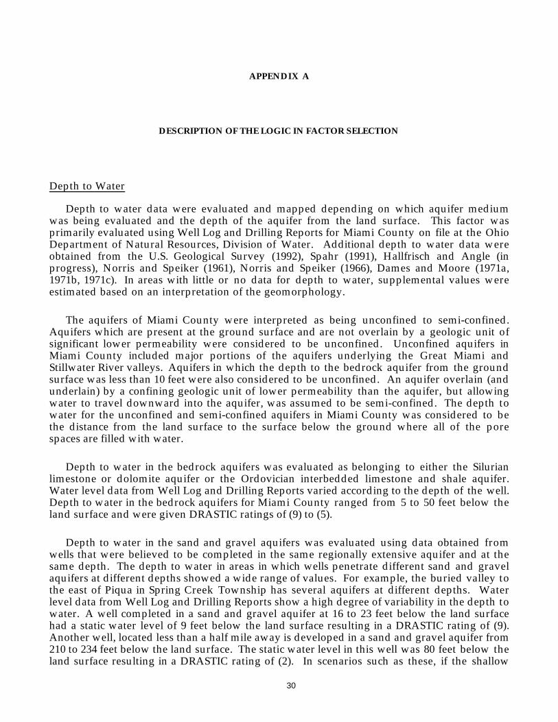
Depth to Water

Depth to water data were evaluated and mapped depending on which aquifer mediumwas being evaluated and the depth of the aquifer from the land surface. This factor wasprimarily evaluated using Well Log and Drilling Reports for Miami County on file at the OhioDepartment of Natural Resources, Division of Water. Additional depth to water data wereobtained from the U.S. Geological Survey (1992), Spahr (1991), Hallfrisch and Angle (inprogress), Norris and Speiker (1961), Norris and Speiker (1966), Dames and Moore (1971a,1971b, 1971c). In areas with little or no data for depth to water, supplemental values wereestimated based on an interpretation of the geomorphology.

The aquifers of Miami County were interpreted as being unconfined to semi-confined.Aquifers which are present at the ground surface and are not overlain by a geologic unit ofsignificant lower permeability were considered to be unconfined. Unconfined aquifers inMiami County included major portions of the aquifers underlying the Great Miami andStillwater River valleys. Aquifers in which the depth to the bedrock aquifer from the groundsurface was less than 10 feet were also considered to be unconfined. An aquifer overlain (andunderlain) by a confining geologic unit of lower permeability than the aquifer, but allowingwater to travel downward into the aquifer, was assumed to be semi-confined. The depth towater for the unconfined and semi-confined aquifers in Miami County was considered to bethe distance from the land surface to the surface below the ground where all of the porespaces are filled with water.

Depth to water in the bedrock aquifers was evaluated as belonging to either the Silurianlimestone or dolomite aquifer or the Ordovician interbedded limestone and shale aquifer.Water level data from Well Log and Drilling Reports varied according to the depth of the well.Depth to water in the bedrock aquifers for Miami County ranged from 5 to 50 feet below theland surface and were given DRASTIC ratings of (9) to (5).

Depth to water in the sand and gravel aquifers was evaluated using data obtained fromwells that were believed to be completed in the same regionally extensive aquifer and at thesame depth. The depth to water in areas in which wells penetrate different sand and gravelaquifers at different depths showed a wide range of values. For example, the buried valley tothe east of Piqua in Spring Creek Township has several aquifers at different depths. Waterlevel data from Well Log and Drilling Reports show a high degree of variability in the depth towater. A well completed in a sand and gravel aquifer at 16 to 23 feet below the land surfacehad a static water level of 9 feet below the land surface resulting in a DRASTIC rating of (9).Another well, located less than a half mile away is developed in a sand and gravel aquifer from210 to 234 feet below the land surface. The static water level in this well was 80 feet below theland surface resulting in a DRASTIC rating of (2). In scenarios such as these, if the shallow

31

aquifer was regionally extensive, the shallower depth to water was generally used for theDRASTIC rating.

Depth to water values for the sand and gravel aquifers in Miami County ranged from 5 to100 feet below the land surface and were given DRASTIC ratings of (9) to (2). Depth to waterfor sand and gravel aquifers adjacent to the floodplains of modern drainage systems rangedfrom 5 to 30 feet below the land surface which correspond to a DRASTIC rating of (9) to (7).Depth to water in areas with deep wells and significant till cover typically had deeper depths towater. Areas mapped as buried valleys (7D) have the broadest range of depth to watervalues. Depth to water ranged from 5 to 100 feet (DRASTIC rating of (9) to (2)) in thishydrogeologic setting.

Net Recharge

As used in the DRASTIC methodology, net recharge is defined as the total quantity ofprecipitation, in inches per year, applied to the ground surface that infiltrates to the aquifer(Aller et al, 1987). Net recharge values were derived from data and information provided inPettyjohn and Henning (1979), Hallfrisch and Angle (in progress), Spahr (1991), Lehman andBottrell (1978), and Well Log and Drilling Reports for wells located in Miami County, Ohio.

The average annual precipitation for Miami County is approximately 37 inches per year.Only a portion of the 37 inches infiltrates the aquifer. The remainder is lost throughevaporation, transpiration, and surficial runoff. The amount of recharge reaching the aquiferis dependent on and influenced by DRASTIC parameters such as topography, vadose zonematerial, and soil type. As the slope of the land surface becomes steeper, the amount of runoffincreases. Therefore, net recharge would be less in steeper areas relative to flatter regions.The amount of recharge to an aquifer system is also influenced by the amount of coarse to finematerial found in the soil and vadose zone. Coarser deposits are more permeable than finerdeposits and will therefore allow a higher percentage of precipatation to infiltrate the aquifersystem.

Areas in Miami County that have a clay loam soil, a significant thick till as a vadose zone,and the Ordovician interbedded limestone and shale as an aquifer were evaluated as receiving2 to 4 inches per year of recharge to the aquifer (DRASTIC rating of (3)). This value wascommon in portions of Miami County mapped as Till over Shale (7Aa). A DRASTIC rating of(3) was given to portions of the Thin Till Over Shale (7G) hydrogeologic setting locatedadjacent to the Stillwater and Great Miami Rivers. This setting typically has a steep slope ofinterbedded limestone and shale of low permeability.

A large portion of various hydrogeologic settings in Miami County was estimated toreceive 4 to 7 inches per year (DRASTIC rating of (6)) of recharge to the underlying aquifers.This rating was also given to settings located in flat areas with a clay loam soil and a till vadosezone. A DRASTIC rating of (6) was given to all of the Sand and Gravel Interbedded in Till(7Af) and Till Over Limestone (7Ac) hydrogeologic settings. A DRASTIC rating of (6) wasgiven to portions of the Till over Shale (7Aa) settings. These areas are flat and have a thinlayer of till as a vadose zone.

32

A net recharge of 7 to 10 inches per year (DRASTIC rating of (8)) was given to flat areas inMiami County with permeable soils and a coarse vadose zone of sand and gravel withsignificant amounts of silt and clay. Areas adjacent to modern drainages were given aDRASTIC recharge value of (8). These areas included large portions of the Buried Valley (7D)setting, Alluvium over Bedded Sedimentary Rock (7Ec) setting, and the Alluvium over Till(7Ed) setting. Outwash over Limestone (7Bc), Outwash over Bedded Sedimentary Rock (7Bb),and Outwash over Till (7Bd) were given a DRASTIC recharge value of (8). Areas mapped asThin Till over Limestone (7Gb) were generally given a DRASTIC rating of (8). These areashave less than ten feet of till over fractured limestone. The tills in this setting were assumed tobe fractured and more permeable than those with greater than ten feet of till.

Aquifer Media

Aquifer media is defined as the consolidated or unconsolidated rock that yields sufficientquantities of water for use (Aller et al., 1987). This parameter was evaluated using dataobtained from field observations by the author, Well Log and Drilling Reports for MiamiCounty on file at the Ohio Department of Natural Resources, and from the following reportsand maps: Dames and Moore (1971a, b, c), Hallfrisch and Angle (in progress), Spahr (1991),Schmidt (1984), Schumacher (1991a, b, c, d, e, f, g, h), Norris and Fidler (1973), Norris andSpeiker (1961), Horvath and Sparling (1967) and Stout et al., (1943).

DRASTIC ratings are assigned to aquifer media based on the degree of fracturing andbedding planes of consolidated bedrock aquifers, and on the degree of sorting and the amountof fine material present in the unconsolidated sand and gravel aquifers. Similar to the rating ofdepth to water, in areas where there is more than one aquifer present, the shallower aquifer isevaluated. The aquifers in Miami County were assumed to be semi-confined to unconfined.

The consolidated bedrock aquifers of Miami County consist of Silurian limestone andOrdivician interbedded limestones and shales. The Silurian limestone aquifer was given aDRASTIC rating of (6) The less permeable Ordovician interbedded limestone and shaleaquifer was given a DRASTIC rating of (3). Bedrock was evaluated as the aquifer media inareas of the county where the overlying material did not contain sufficient amounts of sandand gravel to supply water to domestic wells. The type of aquifer media present wasdelineated using the bedrock geology maps of Shcumacher (1991a, b, c, d, e, f, g, h), theground water resource map of Schmidt (1984), and Well Log and Drilling Reports on file at theOhio Department of Natural Resources.

Limestone was evaluated as the aquifer media for all of the Till Over Limestone (7Ac) andthe Thin Till over Limestone (7Gb) hydrogeologic settings. Portions of the Outwash Over Till(7Bd) setting and Alluvium Over Bedded Sedimentary Rock (7Ec) setting were rated as havinglimestone as the aquifer media.

The interbedded limestone and shale aquifer was evaluated as the media for the Thin Tillover Bedded Sedimentary Rocks (7G) and the Till Over Shale (7Aa) hydrogeologic setting.Portions of the Alluvium Over Bedded Sedimentary Rocks (7Ec) and Outwash Over Till (7Bd)settings were evaluated as having interbedded limestone and shale aquifer media.

33

The unconsolidated sand and gravel aquifers of Miami were given DRASTIC ratings of (6),(7), or (8) depending on the degree of sorting, coarseness, and the composition of the deposit.Sand and gravel aquifers in Miami County are located within buried valleys as valley traindeposits, interbedded in glacial till, and as outwash. The sand and gravel aquifers adjacent tomost reaches of the Stillwater River, the Great Miami River, and Honey Creek generally weregiven higher ratings in comparison to other parts of the county.

Soil Media

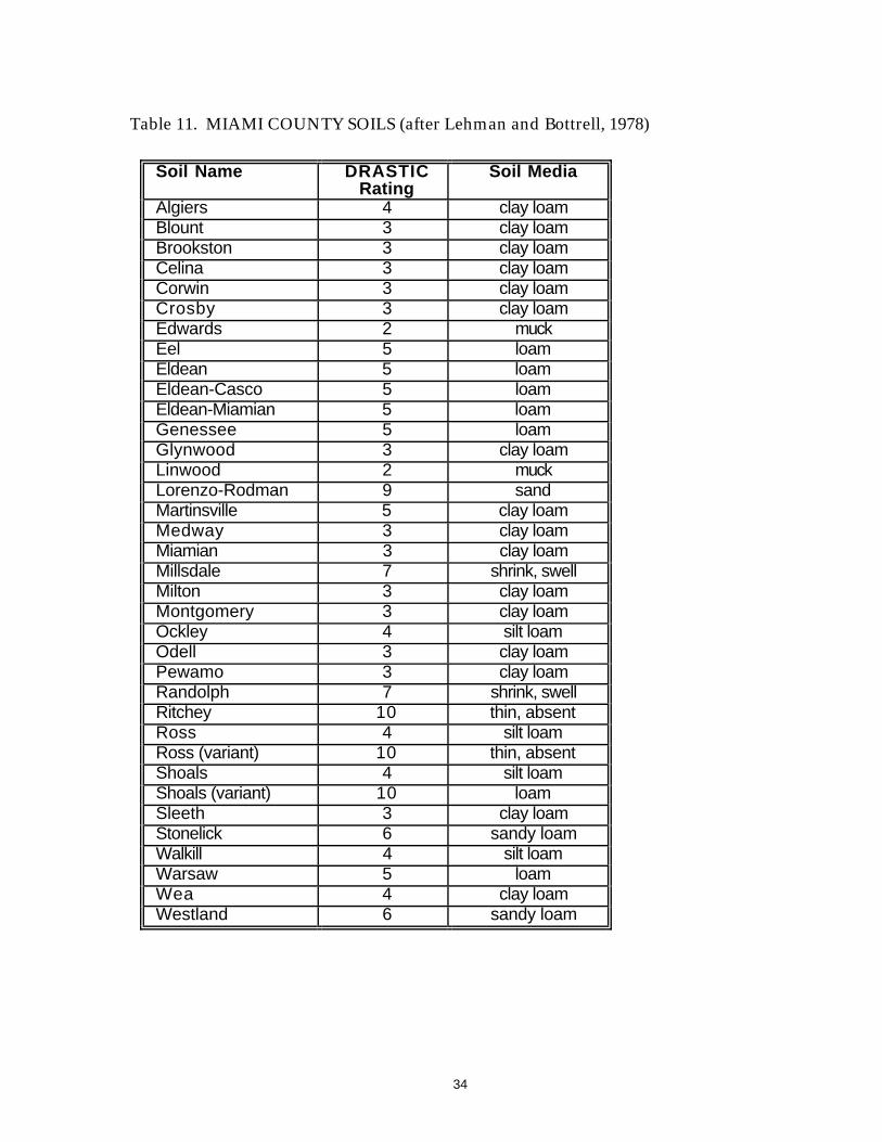
This parameter was evaluated using the soil survey of Miami County, Ohio (Lehman andBottrell, 1978). Each soil was evaluated and given a DRASTIC rating for soil media (Table 11).Evaluations were based on the texture, permeability, and shrink swell potential of each soilunit. DRASTIC ratings for soil media are lower for soils in which the parent material is till thansoils in which parent material is outwash or alluvium.

34

Table 11. MIAMI COUNTY SOILS (after Lehman and Bottrell, 1978)

Soil Name DRASTICRating

Soil Media

Algiers 4 clay loamBlount 3 clay loamBrookston 3 clay loamCelina 3 clay loamCorwin 3 clay loamCrosby 3 clay loamEdwards 2 muckEel 5 loamEldean 5 loamEldean-Casco 5 loamEldean-Miamian 5 loamGenessee 5 loamGlynwood 3 clay loamLinwood 2 muckLorenzo-Rodman 9 sandMartinsville 5 clay loamMedway 3 clay loamMiamian 3 clay loamMillsdale 7 shrink, swellMilton 3 clay loamMontgomery 3 clay loamOckley 4 silt loamOdell 3 clay loamPewamo 3 clay loamRandolph 7 shrink, swellRitchey 10 thin, absentRoss 4 silt loamRoss (variant) 10 thin, absentShoals 4 silt loamShoals (variant) 10 loamSleeth 3 clay loamStonelick 6 sandy loamWalkill 4 silt loamWarsaw 5 loamWea 4 clay loamWestland 6 sandy loam

35

Topography

Topography, or percent slope, was evaluated using USGS 7.5 minute quadrangle maps andthe soil survey of Miami County, Ohio (Lehman and Bottrell, 1978). DRASTIC ratings fortopography ranged from (3) to (10) (12-18 percent to 0-2 percent).

Impact of the Vadose Zone Media

Vadose zone media in Miami County consisted of till, sand and gravel with significant siltand clay, sand and gravel, silt and clay, limestone, and interbedded limestone and shale.Numerical DRASTIC ratings were given based on composition, thickness, and permeability ofthe vadose zone deposits. This parameter was evaluated using information obtained fromHallfrisch and Angle (in progress), Spahr (1991), Forsyth (1965), Lehman and Bottrell (1978),Dames and Moore (1971a,b,c), Well Log and Drilling Reports on file at the Ohio Department ofNatural Resources, and field observations made by the author.

DRASTIC values for vadose zone media in Miami County ranged from (3) to (8). Till,where evaluated as a vadose zone media, was given a DRASTIC rating of (3) for areas to thenortheast of Greenville Creek. A rating of (4) was given to the till vadose zone for theremainder of the county. These ratings were given because the till northeast of GreenvilleCreek and associated with the Union City and Bloomer Moraines are more clay-rich andtherefore less permeable than till in the remainder of the county. Sand and gravel withsignificant silt and clay and silt and clay were evaluated as the vadose for areas that containedoutwash and recent modern alluvium deposits. These areas were generally adjacent to theGreat Miami River, Honey Creek, Greenville Creek, Ludlow Creek, and the Stillwater River.DRASTIC ratings for areas evaluated as having sand and gravel with significant silt and clayranged from (5) to (7). Silt and clay deposits were given a rating of (4) or (5). Sand and gravelas a vadose zone media was generally evaluated in areas that contain coarse outwash deposits.A DRASTIC rating of (8) was generally given to these deposits. In areas that had a smallamount of unconsolidated material over the bedrock, limestone or interbedded limestone andshale was evaluated as the vadose zone media. Limestone was given a DRASTIC rating of (6)and the interbedded limestone and shale was given a rating of (3) for vadose zone.

Hydraulic Conductivity

This parameter was evaluated using data obtained from Dames and Moore (1971a, b, c),Klaer and Associates (1966), Klaer and Associates (1970), URS Consultants (1991), Eastman(1989), Eagon (1973), Norris and Fidler (1973), Norris and Speiker (1961), Norris and Speiker(1966), Schmidt (1987), CH2M Hill (1986), Miami Valley Regional Planning Commission (1990),Spahr (1991), and Hallfrisch and Angle (in progress).

Hydraulic conductivity, the ability of the aquifer media to transmit water, is dependent onthe properties of water and the aquifer. Hydraulic conductivity values for Miami Countywere highly variable due to the anisostropy and heterogeneity of the aquifer systems. Thelowest hydraulic conductivities of aquifer media are in the Ordivician interbedded limestone

36

and shale aquifer. The Ordivician interbedded limestone and shale aquifer was evaluated ashaving hydraulic conductivity values ranging from 1 to 100 gallons per day per square foot(gpd/Ft2). This corresponds to a DRASTIC rating of (1). The Silurian limestone aquifer wasevaluated as having hydraulic conductivity values ranging from 100 to 300 gpd/Ft2 (DRASTICrating of (2)). The sand and gravel aquifers of Miami County have a much higher degree ofvariability in hydraulic conductivity values. Values ranged from 100 to over 2000 gpd/Ft2.Drastic values assigned to these aquifers ranged from (2) to (10). Values for the hydraulicconductivity varied depending on the degree of sorting, coarseness, thickness, and the amountof fine material within the sand and gravel aquifer.

37

APPENDIX B

DESCRIPTION OF HYDROGEOLOGIC SETTINGS AND CHARTS

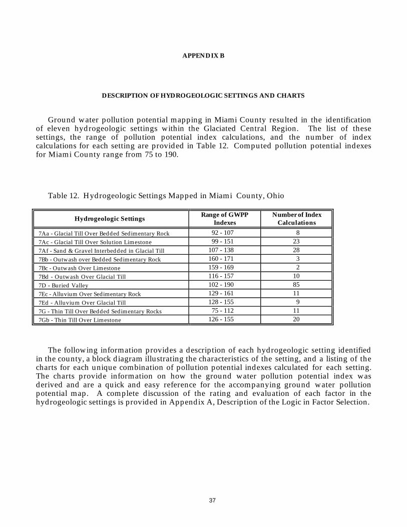
Ground water pollution potential mapping in Miami County resulted in the identificationof eleven hydrogeologic settings within the Glaciated Central Region. The list of thesesettings, the range of pollution potential index calculations, and the number of indexcalculations for each setting are provided in Table 12. Computed pollution potential indexesfor Miami County range from 75 to 190.

Table 12. Hydrogeologic Settings Mapped in Miami County, Ohio

Hydrogeologic SettingsRange of GWPP

IndexesNumber of Index

Calculations

7Aa - Glacial Till Over Bedded Sedimentary Rock 92 - 107 87Ac - Glacial Till Over Solution Limestone 99 - 151 237Af - Sand & Gravel Interbedded in Glacial Till 107 - 138 287Bb - Outwash over Bedded Sedimentary Rock 160 - 171 37Bc - Outwash Over Limestone 159 - 169 27Bd - Outwash Over Glacial Till 116 - 157 107D - Buried Valley 102 - 190 857Ec - Alluvium Over Sedimentary Rock 129 - 161 117Ed - Alluvium Over Glacial Till 128 - 155 97G - Thin Till Over Bedded Sedimentary Rocks 75 - 112 117Gb - Thin Till Over Limestone 126 - 155 20

The following information provides a description of each hydrogeologic setting identifiedin the county, a block diagram illustrating the characteristics of the setting, and a listing of thecharts for each unique combination of pollution potential indexes calculated for each setting.The charts provide information on how the ground water pollution potential index wasderived and are a quick and easy reference for the accompanying ground water pollutionpotential map. A complete discussion of the rating and evaluation of each factor in thehydrogeologic settings is provided in Appendix A, Description of the Logic in Factor Selection.

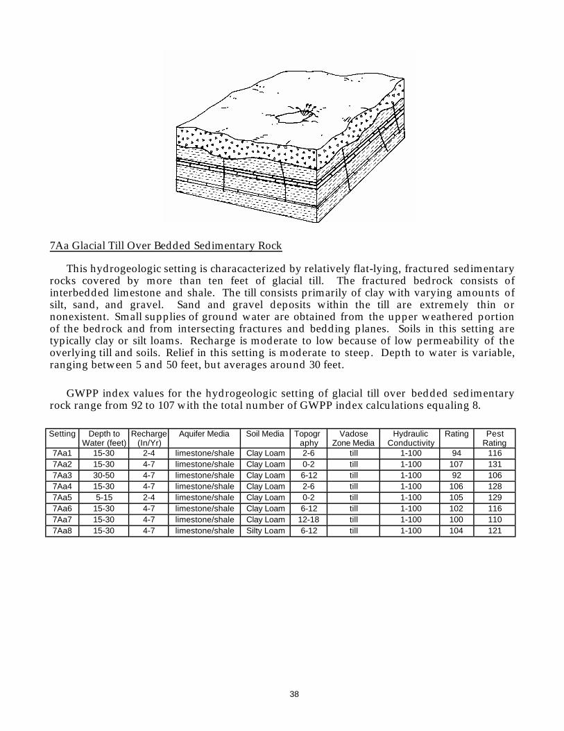
38

7Aa Glacial Till Over Bedded Sedimentary Rock

This hydrogeologic setting is characacterized by relatively flat-lying, fractured sedimentaryrocks covered by more than ten feet of glacial till. The fractured bedrock consists ofinterbedded limestone and shale. The till consists primarily of clay with varying amounts ofsilt, sand, and gravel. Sand and gravel deposits within the till are extremely thin ornonexistent. Small supplies of ground water are obtained from the upper weathered portionof the bedrock and from intersecting fractures and bedding planes. Soils in this setting aretypically clay or silt loams. Recharge is moderate to low because of low permeability of theoverlying till and soils. Relief in this setting is moderate to steep. Depth to water is variable,ranging between 5 and 50 feet, but averages around 30 feet.

GWPP index values for the hydrogeologic setting of glacial till over bedded sedimentaryrock range from 92 to 107 with the total number of GWPP index calculations equaling 8.

Setting Depth toWater (feet)

Recharge(In/Yr)

Aquifer Media Soil Media Topography

VadoseZone Media

HydraulicConductivity

Rating PestRating

7Aa1 15-30 2-4 limestone/shale Clay Loam 2-6 till 1-100 94 1167Aa2 15-30 4-7 limestone/shale Clay Loam 0-2 till 1-100 107 1317Aa3 30-50 4-7 limestone/shale Clay Loam 6-12 till 1-100 92 1067Aa4 15-30 4-7 limestone/shale Clay Loam 2-6 till 1-100 106 1287Aa5 5-15 2-4 limestone/shale Clay Loam 0-2 till 1-100 105 1297Aa6 15-30 4-7 limestone/shale Clay Loam 6-12 till 1-100 102 1167Aa7 15-30 4-7 limestone/shale Clay Loam 12-18 till 1-100 100 1107Aa8 15-30 4-7 limestone/shale Silty Loam 6-12 till 1-100 104 121

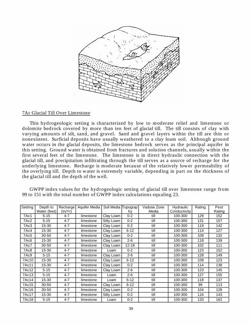
39

7Ac Glacial Till Over Limestone

This hydrogeologic setting is characterized by low to moderate relief and limestone ordolomite bedrock covered by more than ten feet of glacial till. The till consists of clay withvarying amounts of silt, sand, and gravel. Sand and gravel layers within the till are thin ornonexistent. Surficial deposits have usually weathered to a clay loam soil. Although groundwater occurs in the glacial deposits, the limestone bedrock serves as the principal aquifer inthis setting. Ground water is obtained from fractures and solution channels, usually within thefirst several feet of the limestone. The limestone is in direct hydraulic connection with theglacial till, and precipitation infiltrating through the till serves as a source of recharge for theunderlying limestone. Recharge is moderate because of the relatively lower permeability ofthe overlying till. Depth to water is extremely variable, depending in part on the thickness ofthe glacial till and the depth of the well.

GWPP index values for the hydrogeologic setting of glacial till over limestone range from99 to 151 with the total number of GWPP index calculations equaling 23.


Recharge(In/Yr)


Vadose ZoneMedia


Rating PestRating

7Ac1 5-15 4-7 limestone Clay Loam 0-2 till 100-300 129 1527Ac2 5-15 4-7 limestone Silty Loam 0-2 till 100-300 131 1577Ac3 15-30 4-7 limestone Clay Loam 0-2 till 100-300 119 1427Ac4 15-30 4-7 limestone Clay Loam 6-12 till 100-300 114 1277Ac5 30-50 4-7 limestone Clay Loam 0-2 till 100-300 109 1327Ac6 15-30 4-7 limestone Clay Loam 2-6 till 100-300 118 1397Ac7 30-50 4-7 limestone Clay Loam 12-18 till 100-300 102 1117Ac8 15-30 4-7 limestone Loam 0-2 till 100-300 123 1527Ac9 5-15 4-7 limestone Clay Loam 2-6 till 100-300 128 1497Ac10 15-30 4-7 limestone Clay Loam 6-12 till 100-300 109 1237Ac11 15-30 4-7 limestone Clay Loam 0-2 till 100-300 114 1387Ac12 5-15 4-7 limestone Clay Loam 2-6 till 100-300 123 1457Ac13 5-15 4-7 limestone Loam 2-6 till 100-300 127 1557Ac14 15-30 4-7 limestone Loam 6-12 till 100-300 118 1377Ac15 30-50 4-7 limestone Clay Loam 6-12 till 100-300 99 1137Ac16 30-50 4-7 limestone Clay Loam 0-2 till 100-300 104 1287Ac17 15-30 4-7 limestone Silty Loam 0-2 till 100-300 116 1437Ac18 5-15 4-7 limestone Loam 0-2 till 100-300 133 162

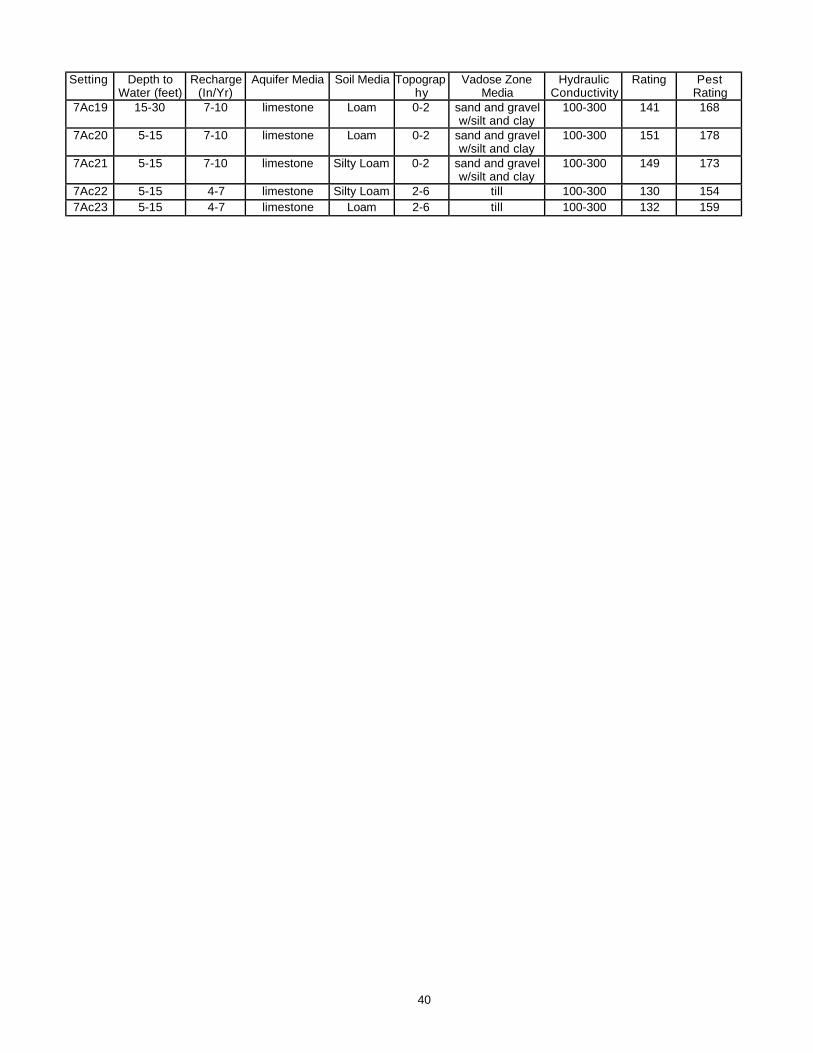
40


Recharge(In/Yr)


Vadose ZoneMedia


Rating PestRating

7Ac19 15-30 7-10 limestone Loam 0-2 sand and gravelw/silt and clay

100-300 141 168

7Ac20 5-15 7-10 limestone Loam 0-2 sand and gravelw/silt and clay

100-300 151 178

7Ac21 5-15 7-10 limestone Silty Loam 0-2 sand and gravelw/silt and clay

100-300 149 173

7Ac22 5-15 4-7 limestone Silty Loam 2-6 till 100-300 130 1547Ac23 5-15 4-7 limestone Loam 2-6 till 100-300 132 159

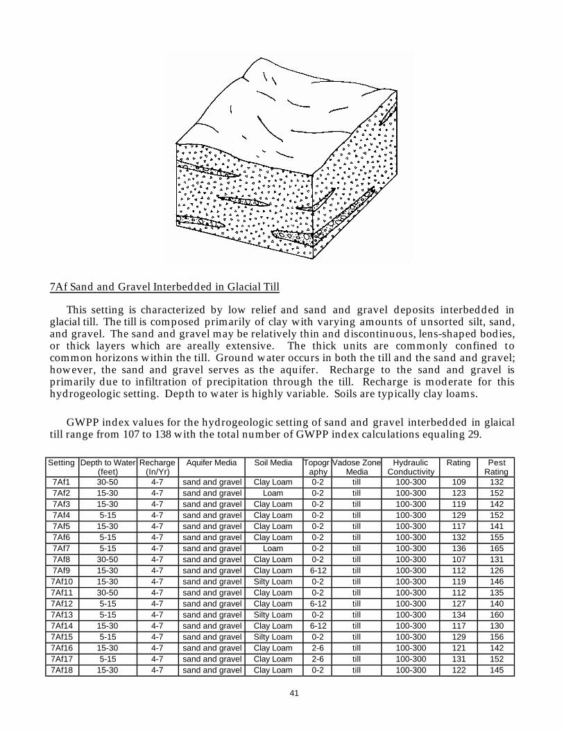
41

7Af Sand and Gravel Interbedded in Glacial Till

This setting is characterized by low relief and sand and gravel deposits interbedded inglacial till. The till is composed primarily of clay with varying amounts of unsorted silt, sand,and gravel. The sand and gravel may be relatively thin and discontinuous, lens-shaped bodies,or thick layers which are areally extensive. The thick units are commonly confined tocommon horizons within the till. Ground water occurs in both the till and the sand and gravel;however, the sand and gravel serves as the aquifer. Recharge to the sand and gravel isprimarily due to infiltration of precipitation through the till. Recharge is moderate for thishydrogeologic setting. Depth to water is highly variable. Soils are typically clay loams.

GWPP index values for the hydrogeologic setting of sand and gravel interbedded in glaicaltill range from 107 to 138 with the total number of GWPP index calculations equaling 29.

Setting Depth to Water(feet)

Recharge(In/Yr)


Vadose ZoneMedia


Rating PestRating

7Af1 30-50 4-7 sand and gravel Clay Loam 0-2 till 100-300 109 1327Af2 15-30 4-7 sand and gravel Loam 0-2 till 100-300 123 1527Af3 15-30 4-7 sand and gravel Clay Loam 0-2 till 100-300 119 1427Af4 5-15 4-7 sand and gravel Clay Loam 0-2 till 100-300 129 1527Af5 15-30 4-7 sand and gravel Clay Loam 0-2 till 100-300 117 1417Af6 5-15 4-7 sand and gravel Clay Loam 0-2 till 100-300 132 1557Af7 5-15 4-7 sand and gravel Loam 0-2 till 100-300 136 1657Af8 30-50 4-7 sand and gravel Clay Loam 0-2 till 100-300 107 1317Af9 15-30 4-7 sand and gravel Clay Loam 6-12 till 100-300 112 1267Af10 15-30 4-7 sand and gravel Silty Loam 0-2 till 100-300 119 1467Af11 30-50 4-7 sand and gravel Clay Loam 0-2 till 100-300 112 1357Af12 5-15 4-7 sand and gravel Clay Loam 6-12 till 100-300 127 1407Af13 5-15 4-7 sand and gravel Silty Loam 0-2 till 100-300 134 1607Af14 15-30 4-7 sand and gravel Clay Loam 6-12 till 100-300 117 1307Af15 5-15 4-7 sand and gravel Silty Loam 0-2 till 100-300 129 1567Af16 15-30 4-7 sand and gravel Clay Loam 2-6 till 100-300 121 1427Af17 5-15 4-7 sand and gravel Clay Loam 2-6 till 100-300 131 1527Af18 15-30 4-7 sand and gravel Clay Loam 0-2 till 100-300 122 145

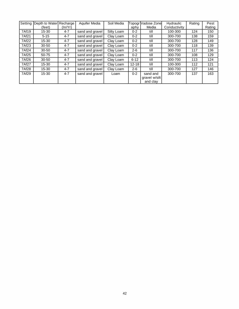
42


Recharge(In/Yr)


Vadose ZoneMedia


Rating PestRating

7Af19 15-30 4-7 sand and gravel Silty Loam 0-2 till 100-300 124 1507Af21 5-15 4-7 sand and gravel Clay Loam 0-2 till 300-700 138 1597Af22 15-30 4-7 sand and gravel Clay Loam 0-2 till 300-700 128 1497Af23 30-50 4-7 sand and gravel Clay Loam 0-2 till 300-700 118 1397Af24 30-50 4-7 sand and gravel Clay Loam 2-6 till 300-700 117 1367Af25 50-75 4-7 sand and gravel Clay Loam 0-2 till 300-700 108 1297Af26 30-50 4-7 sand and gravel Clay Loam 6-12 till 300-700 113 1247Af27 15-30 4-7 sand and gravel Clay Loam 12-18 till 100-300 112 1217Af28 15-30 4-7 sand and gravel Clay Loam 2-6 till 300-700 127 1467Af29 15-30 4-7 sand and gravel Loam 0-2 sand and

gravel w/siltand clay

300-700 137 163

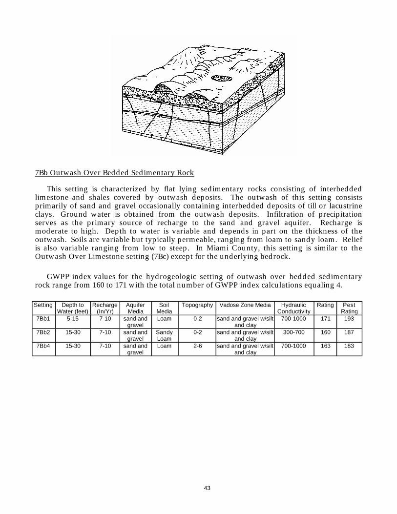
43

7Bb Outwash Over Bedded Sedimentary Rock

This setting is characterized by flat lying sedimentary rocks consisting of interbeddedlimestone and shales covered by outwash deposits. The outwash of this setting consistsprimarily of sand and gravel occasionally containing interbedded deposits of till or lacustrineclays. Ground water is obtained from the outwash deposits. Infiltration of precipitationserves as the primary source of recharge to the sand and gravel aquifer. Recharge ismoderate to high. Depth to water is variable and depends in part on the thickness of theoutwash. Soils are variable but typically permeable, ranging from loam to sandy loam. Reliefis also variable ranging from low to steep. In Miami County, this setting is similar to theOutwash Over Limestone setting (7Bc) except for the underlying bedrock.

GWPP index values for the hydrogeologic setting of outwash over bedded sedimentaryrock range from 160 to 171 with the total number of GWPP index calculations equaling 4.


Recharge(In/Yr)

AquiferMedia

SoilMedia

Topography Vadose Zone Media HydraulicConductivity

Rating PestRating

7Bb1 5-15 7-10 sand andgravel

Loam 0-2 sand and gravel w/siltand clay

700-1000 171 193


SandyLoam

0-2 sand and gravel w/siltand clay

300-700 160 187


Loam 2-6 sand and gravel w/siltand clay

700-1000 163 183

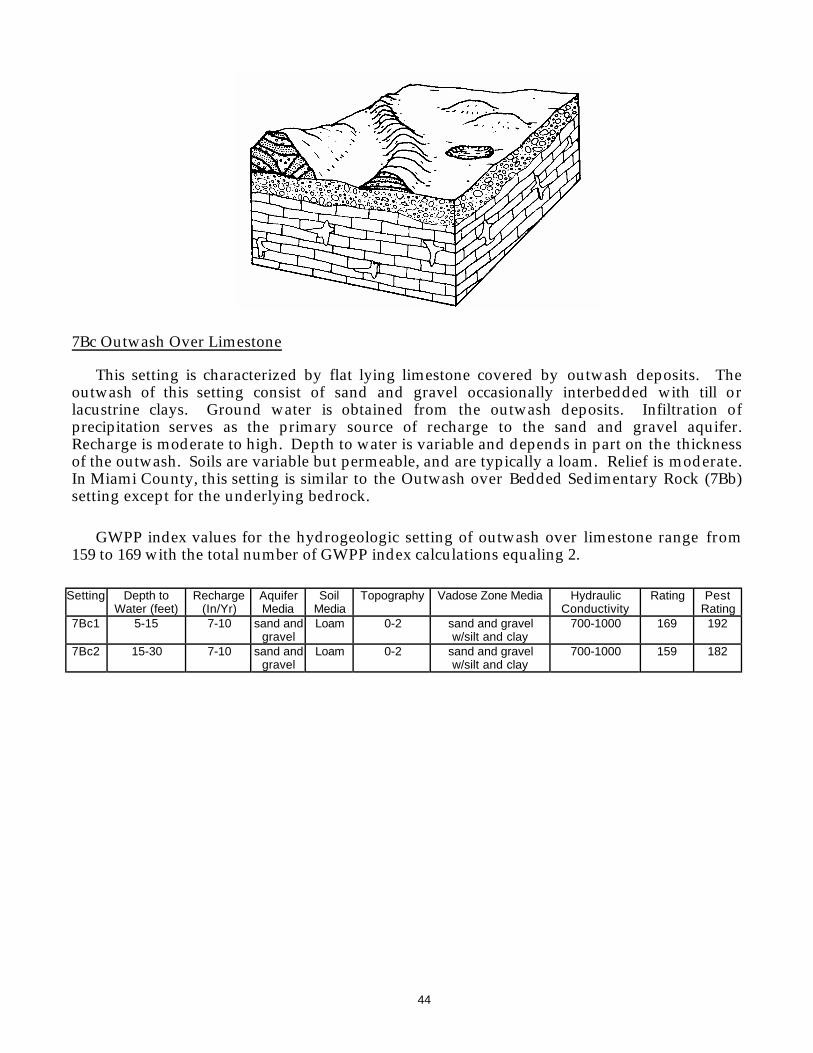
44

7Bc Outwash Over Limestone

This setting is characterized by flat lying limestone covered by outwash deposits. Theoutwash of this setting consist of sand and gravel occasionally interbedded with till orlacustrine clays. Ground water is obtained from the outwash deposits. Infiltration ofprecipitation serves as the primary source of recharge to the sand and gravel aquifer.Recharge is moderate to high. Depth to water is variable and depends in part on the thicknessof the outwash. Soils are variable but permeable, and are typically a loam. Relief is moderate.In Miami County, this setting is similar to the Outwash over Bedded Sedimentary Rock (7Bb)setting except for the underlying bedrock.

GWPP index values for the hydrogeologic setting of outwash over limestone range from159 to 169 with the total number of GWPP index calculations equaling 2.


Recharge(In/Yr)

AquiferMedia

SoilMedia

Topography Vadose Zone Media HydraulicConductivity

Rating PestRating

7Bc1 5-15 7-10 sand andgravel

Loam 0-2 sand and gravelw/silt and clay

700-1000 169 192

7Bc2 15-30 7-10 sand andgravel

Loam 0-2 sand and gravelw/silt and clay

700-1000 159 182

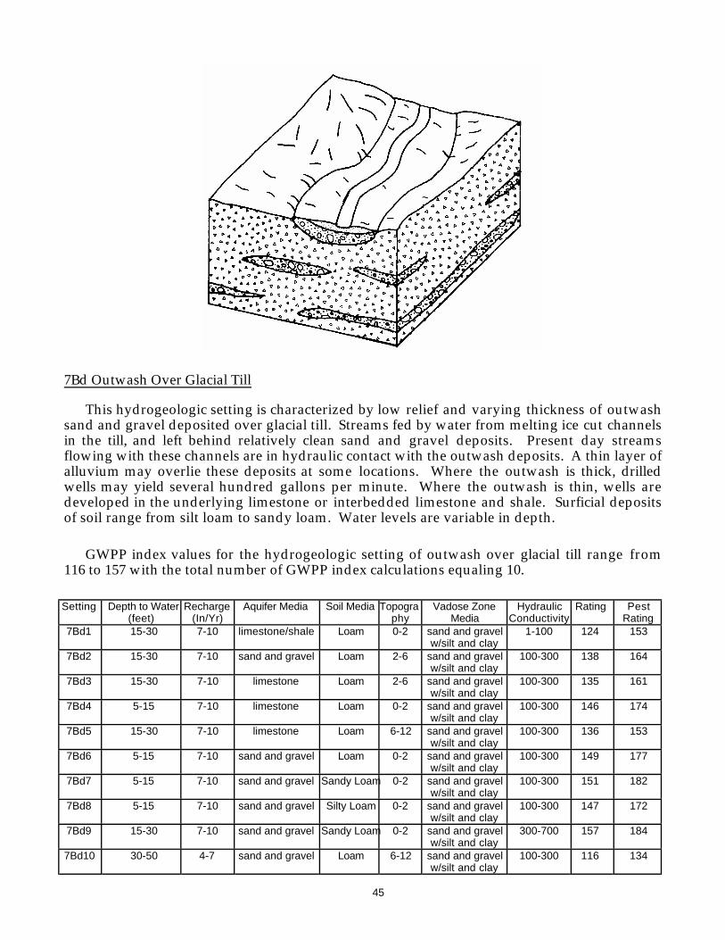
45

7Bd Outwash Over Glacial Till

This hydrogeologic setting is characterized by low relief and varying thickness of outwashsand and gravel deposited over glacial till. Streams fed by water from melting ice cut channelsin the till, and left behind relatively clean sand and gravel deposits. Present day streamsflowing with these channels are in hydraulic contact with the outwash deposits. A thin layer ofalluvium may overlie these deposits at some locations. Where the outwash is thick, drilledwells may yield several hundred gallons per minute. Where the outwash is thin, wells aredeveloped in the underlying limestone or interbedded limestone and shale. Surficial depositsof soil range from silt loam to sandy loam. Water levels are variable in depth.

GWPP index values for the hydrogeologic setting of outwash over glacial till range from116 to 157 with the total number of GWPP index calculations equaling 10.


Recharge(In/Yr)


Vadose ZoneMedia


Rating PestRating

7Bd1 15-30 7-10 limestone/shale Loam 0-2 sand and gravelw/silt and clay

1-100 124 153

7Bd2 15-30 7-10 sand and gravel Loam 2-6 sand and gravelw/silt and clay

100-300 138 164

7Bd3 15-30 7-10 limestone Loam 2-6 sand and gravelw/silt and clay

100-300 135 161


100-300 146 174


100-300 136 153


100-300 149 177

7Bd7 5-15 7-10 sand and gravel Sandy Loam 0-2 sand and gravelw/silt and clay

100-300 151 182

7Bd8 5-15 7-10 sand and gravel Silty Loam 0-2 sand and gravelw/silt and clay

100-300 147 172

7Bd9 15-30 7-10 sand and gravel Sandy Loam 0-2 sand and gravelw/silt and clay

300-700 157 184


100-300 116 134

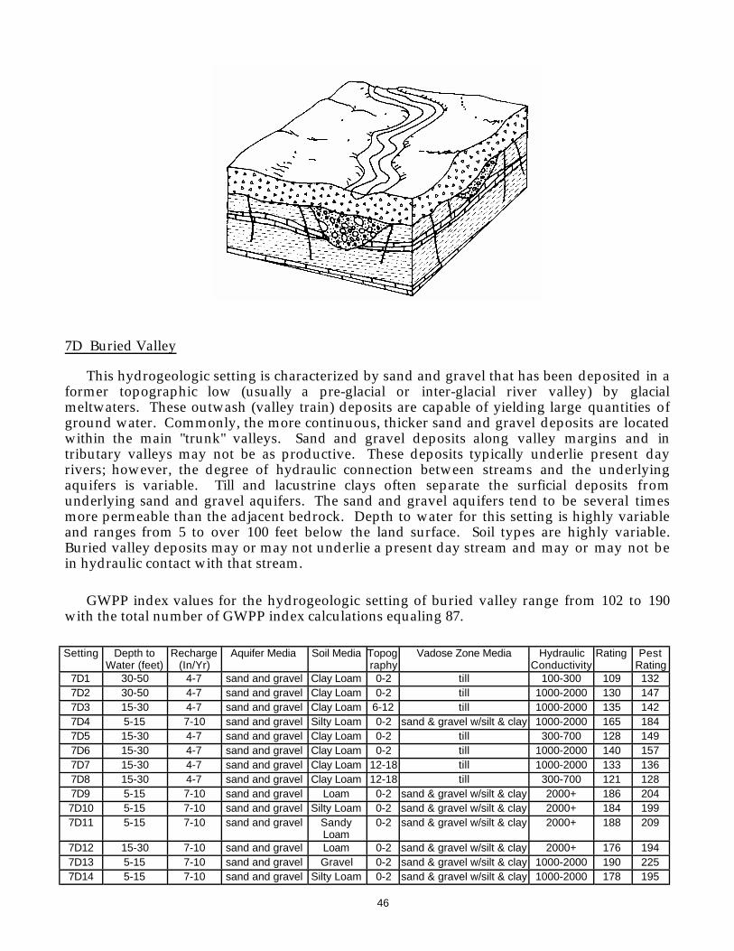
46

7D Buried Valley

This hydrogeologic setting is characterized by sand and gravel that has been deposited in aformer topographic low (usually a pre-glacial or inter-glacial river valley) by glacialmeltwaters. These outwash (valley train) deposits are capable of yielding large quantities ofground water. Commonly, the more continuous, thicker sand and gravel deposits are locatedwithin the main "trunk" valleys. Sand and gravel deposits along valley margins and intributary valleys may not be as productive. These deposits typically underlie present dayrivers; however, the degree of hydraulic connection between streams and the underlyingaquifers is variable. Till and lacustrine clays often separate the surficial deposits fromunderlying sand and gravel aquifers. The sand and gravel aquifers tend to be several timesmore permeable than the adjacent bedrock. Depth to water for this setting is highly variableand ranges from 5 to over 100 feet below the land surface. Soil types are highly variable.Buried valley deposits may or may not underlie a present day stream and may or may not bein hydraulic contact with that stream.

GWPP index values for the hydrogeologic setting of buried valley range from 102 to 190with the total number of GWPP index calculations equaling 87.


Recharge(In/Yr)


Vadose Zone Media HydraulicConductivity

Rating PestRating

7D1 30-50 4-7 sand and gravel Clay Loam 0-2 till 100-300 109 1327D2 30-50 4-7 sand and gravel Clay Loam 0-2 till 1000-2000 130 1477D3 15-30 4-7 sand and gravel Clay Loam 6-12 till 1000-2000 135 1427D4 5-15 7-10 sand and gravel Silty Loam 0-2 sand & gravel w/silt & clay 1000-2000 165 1847D5 15-30 4-7 sand and gravel Clay Loam 0-2 till 300-700 128 1497D6 15-30 4-7 sand and gravel Clay Loam 0-2 till 1000-2000 140 1577D7 15-30 4-7 sand and gravel Clay Loam 12-18 till 1000-2000 133 1367D8 15-30 4-7 sand and gravel Clay Loam 12-18 till 300-700 121 1287D9 5-15 7-10 sand and gravel Loam 0-2 sand & gravel w/silt & clay 2000+ 186 2047D10 5-15 7-10 sand and gravel Silty Loam 0-2 sand & gravel w/silt & clay 2000+ 184 1997D11 5-15 7-10 sand and gravel Sandy

Loam0-2 sand & gravel w/silt & clay 2000+ 188 209

7D12 15-30 7-10 sand and gravel Loam 0-2 sand & gravel w/silt & clay 2000+ 176 1947D13 5-15 7-10 sand and gravel Gravel 0-2 sand & gravel w/silt & clay 1000-2000 190 2257D14 5-15 7-10 sand and gravel Silty Loam 0-2 sand & gravel w/silt & clay 1000-2000 178 195

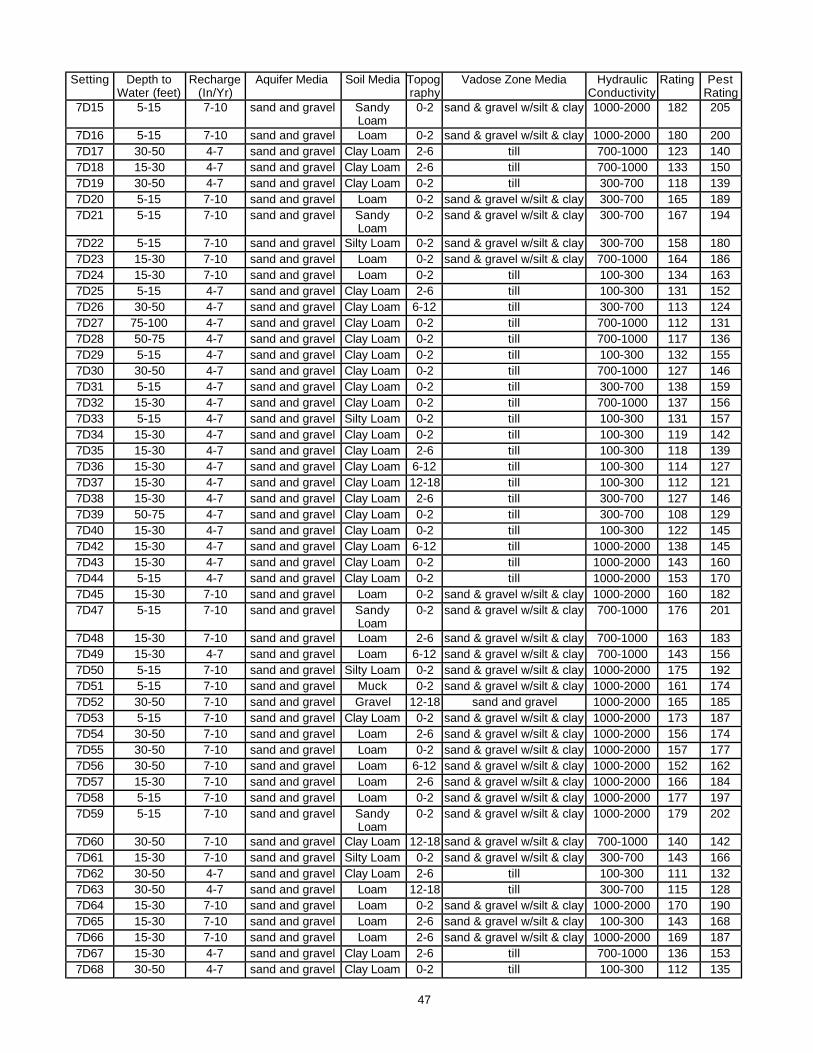
47


Recharge(In/Yr)



Rating PestRating

7D15 5-15 7-10 sand and gravel SandyLoam

0-2 sand & gravel w/silt & clay 1000-2000 182 205

7D16 5-15 7-10 sand and gravel Loam 0-2 sand & gravel w/silt & clay 1000-2000 180 2007D17 30-50 4-7 sand and gravel Clay Loam 2-6 till 700-1000 123 1407D18 15-30 4-7 sand and gravel Clay Loam 2-6 till 700-1000 133 1507D19 30-50 4-7 sand and gravel Clay Loam 0-2 till 300-700 118 1397D20 5-15 7-10 sand and gravel Loam 0-2 sand & gravel w/silt & clay 300-700 165 1897D21 5-15 7-10 sand and gravel Sandy

Loam0-2 sand & gravel w/silt & clay 300-700 167 194

7D22 5-15 7-10 sand and gravel Silty Loam 0-2 sand & gravel w/silt & clay 300-700 158 1807D23 15-30 7-10 sand and gravel Loam 0-2 sand & gravel w/silt & clay 700-1000 164 1867D24 15-30 7-10 sand and gravel Loam 0-2 till 100-300 134 1637D25 5-15 4-7 sand and gravel Clay Loam 2-6 till 100-300 131 1527D26 30-50 4-7 sand and gravel Clay Loam 6-12 till 300-700 113 1247D27 75-100 4-7 sand and gravel Clay Loam 0-2 till 700-1000 112 1317D28 50-75 4-7 sand and gravel Clay Loam 0-2 till 700-1000 117 1367D29 5-15 4-7 sand and gravel Clay Loam 0-2 till 100-300 132 1557D30 30-50 4-7 sand and gravel Clay Loam 0-2 till 700-1000 127 1467D31 5-15 4-7 sand and gravel Clay Loam 0-2 till 300-700 138 1597D32 15-30 4-7 sand and gravel Clay Loam 0-2 till 700-1000 137 1567D33 5-15 4-7 sand and gravel Silty Loam 0-2 till 100-300 131 1577D34 15-30 4-7 sand and gravel Clay Loam 0-2 till 100-300 119 1427D35 15-30 4-7 sand and gravel Clay Loam 2-6 till 100-300 118 1397D36 15-30 4-7 sand and gravel Clay Loam 6-12 till 100-300 114 1277D37 15-30 4-7 sand and gravel Clay Loam 12-18 till 100-300 112 1217D38 15-30 4-7 sand and gravel Clay Loam 2-6 till 300-700 127 1467D39 50-75 4-7 sand and gravel Clay Loam 0-2 till 300-700 108 1297D40 15-30 4-7 sand and gravel Clay Loam 0-2 till 100-300 122 1457D42 15-30 4-7 sand and gravel Clay Loam 6-12 till 1000-2000 138 1457D43 15-30 4-7 sand and gravel Clay Loam 0-2 till 1000-2000 143 1607D44 5-15 4-7 sand and gravel Clay Loam 0-2 till 1000-2000 153 1707D45 15-30 7-10 sand and gravel Loam 0-2 sand & gravel w/silt & clay 1000-2000 160 1827D47 5-15 7-10 sand and gravel Sandy


7D48 15-30 7-10 sand and gravel Loam 2-6 sand & gravel w/silt & clay 700-1000 163 1837D49 15-30 4-7 sand and gravel Loam 6-12 sand & gravel w/silt & clay 700-1000 143 1567D50 5-15 7-10 sand and gravel Silty Loam 0-2 sand & gravel w/silt & clay 1000-2000 175 1927D51 5-15 7-10 sand and gravel Muck 0-2 sand & gravel w/silt & clay 1000-2000 161 1747D52 30-50 7-10 sand and gravel Gravel 12-18 sand and gravel 1000-2000 165 1857D53 5-15 7-10 sand and gravel Clay Loam 0-2 sand & gravel w/silt & clay 1000-2000 173 1877D54 30-50 7-10 sand and gravel Loam 2-6 sand & gravel w/silt & clay 1000-2000 156 1747D55 30-50 7-10 sand and gravel Loam 0-2 sand & gravel w/silt & clay 1000-2000 157 1777D56 30-50 7-10 sand and gravel Loam 6-12 sand & gravel w/silt & clay 1000-2000 152 1627D57 15-30 7-10 sand and gravel Loam 2-6 sand & gravel w/silt & clay 1000-2000 166 1847D58 5-15 7-10 sand and gravel Loam 0-2 sand & gravel w/silt & clay 1000-2000 177 1977D59 5-15 7-10 sand and gravel Sandy


7D60 30-50 7-10 sand and gravel Clay Loam 12-18 sand & gravel w/silt & clay 700-1000 140 1427D61 15-30 7-10 sand and gravel Silty Loam 0-2 sand & gravel w/silt & clay 300-700 143 1667D62 30-50 4-7 sand and gravel Clay Loam 2-6 till 100-300 111 1327D63 30-50 4-7 sand and gravel Loam 12-18 till 300-700 115 1287D64 15-30 7-10 sand and gravel Loam 0-2 sand & gravel w/silt & clay 1000-2000 170 1907D65 15-30 7-10 sand and gravel Loam 2-6 sand & gravel w/silt & clay 100-300 143 1687D66 15-30 7-10 sand and gravel Loam 2-6 sand & gravel w/silt & clay 1000-2000 169 1877D67 15-30 4-7 sand and gravel Clay Loam 2-6 till 700-1000 136 1537D68 30-50 4-7 sand and gravel Clay Loam 0-2 till 100-300 112 135

48


Recharge(In/Yr)



Rating PestRating

7D69 15-30 4-7 sand and gravel Clay Loam 0-2 till 300-700 128 1497D70 5-15 4-7 sand and gravel Loam 0-2 sand & gravel w/silt & clay 1000-2000 162 1847D71 30-50 4-7 sand and gravel Clay Loam 2-6 till 700-1000 126 1437D72 15-30 7-10 sand and gravel Loam 0-2 sand & gravel w/silt & clay 700-1000 154 1787D73 30-50 4-7 sand and gravel Clay Loam 0-2 till 100-300 107 1317D74 15-30 4-7 sand and gravel Clay Loam 6-12 till 100-300 112 1267D75 15-30 4-7 sand and gravel Clay Loam 0-2 till 100-300 117 1417D76 30-50 4-7 sand and gravel Clay Loam 6-12 till 100-300 102 1167D77 15-30 4-7 sand and gravel Clay Loam 2-6 till 100-300 116 1387D78 5-15 7-10 sand and gravel Loam 0-2 sand & gravel w/silt & clay 300-700 160 1857D79 15-30 4-7 sand and gravel Loam 0-2 sand & gravel w/silt & clay 100-300 136 1637D80 15-30 4-7 sand and gravel Clay Loam 6-12 till 100-300 109 1237D81 5-15 7-10 sand and gravel Loam 0-2 sand & gravel w/silt & clay 100-300 151 1787D82 5-15 7-10 sand and gravel Silty Loam 0-2 sand & gravel w/silt & clay 100-300 149 1737D83 15-30 4-7 sand and gravel Clay Loam 0-2 till 300-700 123 1457D84 15-30 4-7 sand and gravel Clay Loam 2-6 till 300-700 122 1427D85 15-30 4-7 sand and gravel Clay Loam 0-2 till 100-300 114 1387D86 15-30 4-7 sand and gravel Clay Loam 6-12 till 300-700 118 1307D87 75-100 4-7 sand and gravel Clay Loam 0-2 till 300-700 103 124

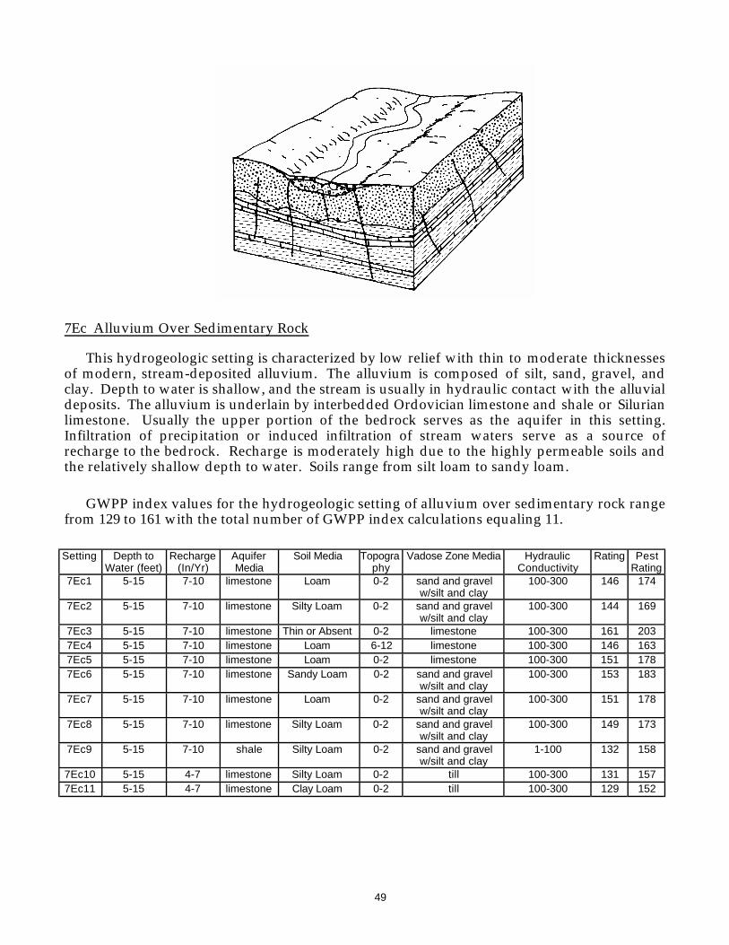
49

7Ec Alluvium Over Sedimentary Rock

This hydrogeologic setting is characterized by low relief with thin to moderate thicknessesof modern, stream-deposited alluvium. The alluvium is composed of silt, sand, gravel, andclay. Depth to water is shallow, and the stream is usually in hydraulic contact with the alluvialdeposits. The alluvium is underlain by interbedded Ordovician limestone and shale or Silurianlimestone. Usually the upper portion of the bedrock serves as the aquifer in this setting.Infiltration of precipitation or induced infiltration of stream waters serve as a source ofrecharge to the bedrock. Recharge is moderately high due to the highly permeable soils andthe relatively shallow depth to water. Soils range from silt loam to sandy loam.

GWPP index values for the hydrogeologic setting of alluvium over sedimentary rock rangefrom 129 to 161 with the total number of GWPP index calculations equaling 11.


Recharge(In/Yr)

AquiferMedia

Soil Media Topography


Rating PestRating

7Ec1 5-15 7-10 limestone Loam 0-2 sand and gravelw/silt and clay

100-300 146 174

7Ec2 5-15 7-10 limestone Silty Loam 0-2 sand and gravelw/silt and clay

100-300 144 169

7Ec3 5-15 7-10 limestone Thin or Absent 0-2 limestone 100-300 161 2037Ec4 5-15 7-10 limestone Loam 6-12 limestone 100-300 146 1637Ec5 5-15 7-10 limestone Loam 0-2 limestone 100-300 151 1787Ec6 5-15 7-10 limestone Sandy Loam 0-2 sand and gravel

w/silt and clay100-300 153 183

7Ec7 5-15 7-10 limestone Loam 0-2 sand and gravelw/silt and clay

100-300 151 178

7Ec8 5-15 7-10 limestone Silty Loam 0-2 sand and gravelw/silt and clay

100-300 149 173

7Ec9 5-15 7-10 shale Silty Loam 0-2 sand and gravelw/silt and clay

1-100 132 158

7Ec10 5-15 4-7 limestone Silty Loam 0-2 till 100-300 131 1577Ec11 5-15 4-7 limestone Clay Loam 0-2 till 100-300 129 152

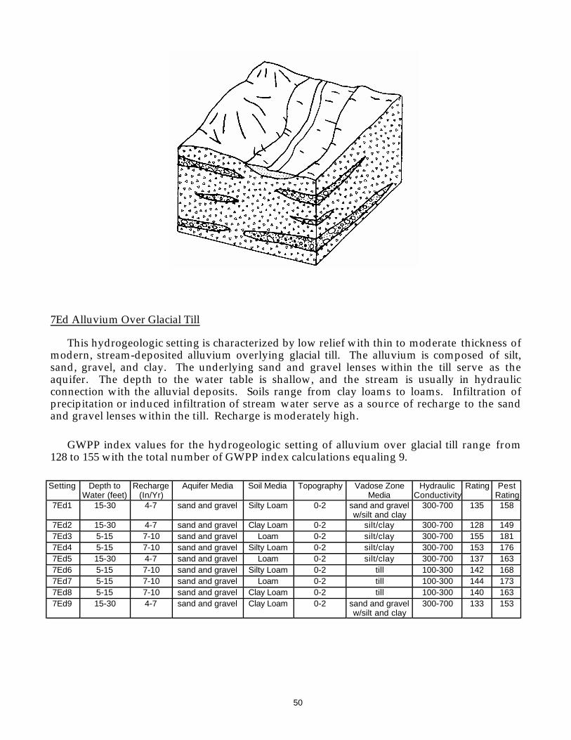
50

7Ed Alluvium Over Glacial Till

This hydrogeologic setting is characterized by low relief with thin to moderate thickness ofmodern, stream-deposited alluvium overlying glacial till. The alluvium is composed of silt,sand, gravel, and clay. The underlying sand and gravel lenses within the till serve as theaquifer. The depth to the water table is shallow, and the stream is usually in hydraulicconnection with the alluvial deposits. Soils range from clay loams to loams. Infiltration ofprecipitation or induced infiltration of stream water serve as a source of recharge to the sandand gravel lenses within the till. Recharge is moderately high.

GWPP index values for the hydrogeologic setting of alluvium over glacial till range from128 to 155 with the total number of GWPP index calculations equaling 9.


Recharge(In/Yr)

Aquifer Media Soil Media Topography Vadose ZoneMedia


Rating PestRating

7Ed1 15-30 4-7 sand and gravel Silty Loam 0-2 sand and gravelw/silt and clay

300-700 135 158

7Ed2 15-30 4-7 sand and gravel Clay Loam 0-2 silt/clay 300-700 128 1497Ed3 5-15 7-10 sand and gravel Loam 0-2 silt/clay 300-700 155 1817Ed4 5-15 7-10 sand and gravel Silty Loam 0-2 silt/clay 300-700 153 1767Ed5 15-30 4-7 sand and gravel Loam 0-2 silt/clay 300-700 137 1637Ed6 5-15 7-10 sand and gravel Silty Loam 0-2 till 100-300 142 1687Ed7 5-15 7-10 sand and gravel Loam 0-2 till 100-300 144 1737Ed8 5-15 7-10 sand and gravel Clay Loam 0-2 till 100-300 140 1637Ed9 15-30 4-7 sand and gravel Clay Loam 0-2 sand and gravel

w/silt and clay300-700 133 153

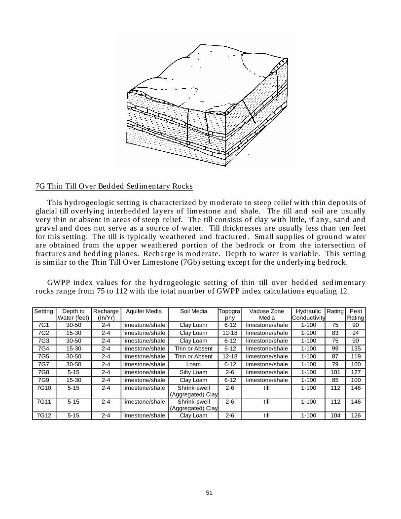
51

7G Thin Till Over Bedded Sedimentary Rocks

This hydrogeologic setting is characterized by moderate to steep relief with thin deposits ofglacial till overlying interbedded layers of limestone and shale. The till and soil are usuallyvery thin or absent in areas of steep relief. The till consists of clay with little, if any, sand andgravel and does not serve as a source of water. Till thicknesses are usually less than ten feetfor this setting. The till is typically weathered and fractured. Small supplies of ground waterare obtained from the upper weathered portion of the bedrock or from the intersection offractures and bedding planes. Recharge is moderate. Depth to water is variable. This settingis similar to the Thin Till Over Limestone (7Gb) setting except for the underlying bedrock.

GWPP index values for the hydrogeologic setting of thin till over bedded sedimentaryrocks range from 75 to 112 with the total number of GWPP index calculations equaling 12.


Recharge(In/Yr)


Vadose ZoneMedia


Rating PestRating

7G1 30-50 2-4 limestone/shale Clay Loam 6-12 limestone/shale 1-100 75 907G2 15-30 2-4 limestone/shale Clay Loam 12-18 limestone/shale 1-100 83 947G3 30-50 2-4 limestone/shale Clay Loam 6-12 limestone/shale 1-100 75 907G4 15-30 2-4 limestone/shale Thin or Absent 6-12 limestone/shale 1-100 99 1357G5 30-50 2-4 limestone/shale Thin or Absent 12-18 limestone/shale 1-100 87 1197G7 30-50 2-4 limestone/shale Loam 6-12 limestone/shale 1-100 79 1007G8 5-15 2-4 limestone/shale Silty Loam 2-6 limestone/shale 1-100 101 1277G9 15-30 2-4 limestone/shale Clay Loam 6-12 limestone/shale 1-100 85 1007G10 5-15 2-4 limestone/shale Shrink-swell

(Aggregated) Clay2-6 till 1-100 112 146

7G11 5-15 2-4 limestone/shale Shrink-swell(Aggregated) Clay

2-6 till 1-100 112 146

7G12 5-15 2-4 limestone/shale Clay Loam 2-6 till 1-100 104 126

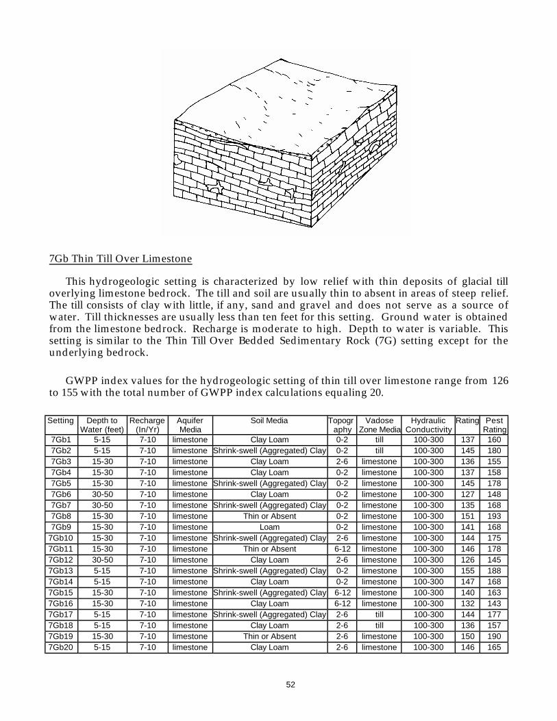
52

7Gb Thin Till Over Limestone

This hydrogeologic setting is characterized by low relief with thin deposits of glacial tilloverlying limestone bedrock. The till and soil are usually thin to absent in areas of steep relief.The till consists of clay with little, if any, sand and gravel and does not serve as a source ofwater. Till thicknesses are usually less than ten feet for this setting. Ground water is obtainedfrom the limestone bedrock. Recharge is moderate to high. Depth to water is variable. Thissetting is similar to the Thin Till Over Bedded Sedimentary Rock (7G) setting except for theunderlying bedrock.

GWPP index values for the hydrogeologic setting of thin till over limestone range from 126to 155 with the total number of GWPP index calculations equaling 20.


Recharge(In/Yr)

AquiferMedia

Soil Media Topography

VadoseZone Media


Rating PestRating

7Gb1 5-15 7-10 limestone Clay Loam 0-2 till 100-300 137 1607Gb2 5-15 7-10 limestone Shrink-swell (Aggregated) Clay 0-2 till 100-300 145 1807Gb3 15-30 7-10 limestone Clay Loam 2-6 limestone 100-300 136 1557Gb4 15-30 7-10 limestone Clay Loam 0-2 limestone 100-300 137 1587Gb5 15-30 7-10 limestone Shrink-swell (Aggregated) Clay 0-2 limestone 100-300 145 1787Gb6 30-50 7-10 limestone Clay Loam 0-2 limestone 100-300 127 1487Gb7 30-50 7-10 limestone Shrink-swell (Aggregated) Clay 0-2 limestone 100-300 135 1687Gb8 15-30 7-10 limestone Thin or Absent 0-2 limestone 100-300 151 1937Gb9 15-30 7-10 limestone Loam 0-2 limestone 100-300 141 168

7Gb10 15-30 7-10 limestone Shrink-swell (Aggregated) Clay 2-6 limestone 100-300 144 1757Gb11 15-30 7-10 limestone Thin or Absent 6-12 limestone 100-300 146 1787Gb12 30-50 7-10 limestone Clay Loam 2-6 limestone 100-300 126 1457Gb13 5-15 7-10 limestone Shrink-swell (Aggregated) Clay 0-2 limestone 100-300 155 1887Gb14 5-15 7-10 limestone Clay Loam 0-2 limestone 100-300 147 1687Gb15 15-30 7-10 limestone Shrink-swell (Aggregated) Clay 6-12 limestone 100-300 140 1637Gb16 15-30 7-10 limestone Clay Loam 6-12 limestone 100-300 132 1437Gb17 5-15 7-10 limestone Shrink-swell (Aggregated) Clay 2-6 till 100-300 144 1777Gb18 5-15 7-10 limestone Clay Loam 2-6 till 100-300 136 1577Gb19 15-30 7-10 limestone Thin or Absent 2-6 limestone 100-300 150 1907Gb20 5-15 7-10 limestone Clay Loam 2-6 limestone 100-300 146 165

53

ERRATA SHEETSeptember 2005

MIAMI COUNTYGround Water Pollution Potential Report No. 27

The following settings have been omitted from the setting tables and do not appear on themap.

7Af20; 7Bb3; 7D41, 7D46; 7G6.

ground water pollution potential of … water pollution potential of miami county, ohio by paul n....

Documents